An integrated model of soil-canopy spectral radiances,photosynthesis, fluorescence, temperature and energy balance
C. van der Tol1, W. Verhoef1, J. Timmermans1, A. Verhoef2, and Z. Su1
1ITC International Institute for Geo-Information Science and Earth Observations, Hengelosestraat 99, P.O. Box 6, 7500 AA,Enschede, The Netherlands2Department of Soil Science, The University of Reading, Whiteknights, Reading, RG6 6DW, UK
Received: 20 May 2009 – Published in Biogeosciences Discuss.: 23 June 2009Revised: 8 November 2009 – Accepted: 25 November 2009 – Published: 18 December 2009
Abstract. This paper presents the model SCOPE (SoilCanopy Observation, Photochemistry and Energy fluxes),which is a vertical (1-D) integrated radiative transfer and en-ergy balance model. The model links visible to thermal in-frared radiance spectra (0.4 to 50 µm) as observed above thecanopy to the fluxes of water, heat and carbon dioxide, as afunction of vegetation structure, and the vertical profiles oftemperature. Output of the model is the spectrum of outgo-ing radiation in the viewing direction and the turbulent heatfluxes, photosynthesis and chlorophyll fluorescence. A spe-cial routine is dedicated to the calculation of photosynthesisrate and chlorophyll fluorescence at the leaf level as a func-tion of net radiation and leaf temperature. The fluorescencecontributions from individual leaves are integrated over thecanopy layer to calculate top-of-canopy fluorescence. Thecalculation of radiative transfer and the energy balance isfully integrated, allowing for feedback between leaf tempera-tures, leaf chlorophyll fluorescence and radiative fluxes. Leaftemperatures are calculated on the basis of energy balanceclosure. Model simulations were evaluated against observa-tions reported in the literature and against data collected dur-ing field campaigns. These evaluations showed that SCOPEis able to reproduce realistic radiance spectra, directional ra-diance and energy balance fluxes. The model may be appliedfor the design of algorithms for the retrieval of evapotranspi-ration from optical and thermal earth observation data, forvalidation of existing methods to monitor vegetation func-tioning, to help interpret canopy fluorescence measurements,and to study the relationships between synoptic observationswith diurnally integrated quantities. The model has been im-plemented in Matlab and has a modular design, thus allowingfor great flexibility and scalability.
Knowledge of physical processes at the land surface is rele-vant for a wide range of applications including weather andclimate prediction, agriculture, and ecological and hydrolog-ical studies. Of particular importance are the fluxes of en-ergy, carbon dioxide and water vapour between land and at-mosphere.
During the last decades scientific understanding of physi-cal processes at the land surface has grown, as a result of theincreased availability of data, both from ground based andremote sensors. The implementation of a network of fluxtowers (FLUXNET) has increased the knowledge about pro-cesses at plot level in different ecosystems and different cli-mates (Baldocchi, 2003). The knowledge from FLUXNETand earlier tower experiments has been widely incorporatedin detailed coupled models for energy, carbon dioxide andwater transport between soil, vegetation and atmosphere(e.g. Sellers et al., 1997; Verhoef and Allen, 2000; Tuzet etal., 2003).
Data from high resolution optical imagers, multi-spectralradiometers and radar on satellite platforms are nowadaysavailable to retrieve spatial information about topography,soil and vegetation (CEOS, 2008). For example, Verhoefand Bach (2003) derived vegetation parameters by invertinga radiative transfer model on satellite derived hyperspectralreflectance data. Attempts have also been made to estimateevaporation from thermal images (Bastiaanssen, 1998). Fur-thermore, remote sensing (RS) data have been used as inputfor spatial soil-vegetation-atmosphere-transfer (SVAT) mod-els for estimation of the surface energy balance (Kustas et al.,1994; Su, 2002; Anderson et al., 2008).
The potential of remote sensors operating at different spa-tial, temporal and spectral resolution is not yet fully ex-ploited, for various reasons. First, remote sensing data is of-ten of too coarse spatial resolution for SVAT models, which
Published by Copernicus Publications on behalf of the European Geosciences Union.
3110 C. van der Tol et al.: An integrated model of soil-canopy spectral radiance observations
are detailed and require field-scale data (Hall et al., 1992).Second, the relation between radiative transfer parametersand SVAT parameters is often indirect, due to their differentscholarly background. For this reason it is not possible to di-rectly translate, for example, an optical leaf area index whichwas successfully retrieved from a radiative transfer modelinto a one-sided leaf area index that is used in a photosyn-thesis model (Norman and Becker, 1995).
In order to make effective use of the available RS data, co-herent models are needed for the interpretation of observedradiance spectra with respect to physical processes on theground. These models should incorporate fluxes of water,carbon and energy at the land surface, as well as radiativetransfer. The model of Goudriaan (1977) and the CUPIDmodel (Norman, 1979; Kustas et al., 2007), to our knowl-edge, have been the first models for both radiative trans-fer and heat, water (vapour) and CO2 exchange in canopies.With these models, brightness temperature can be calculatedfor multiple-source canopies where leaves and soil have dif-ferent temperatures. The models calculate radiation and en-ergy fluxes in forward mode, which means that for the inter-pretation of observed spectra, they have to be inverted.
This paper presents a new model; SCOPE (Soil CanopyObservation of Photochemistry and Energy fluxes), which isa vertical (1-D) integrated radiative transfer and energy bal-ance model. It calculates the spectral radiation regime andthe energy balance of a vegetated surface at the level of sin-gle leaves as well as at canopy level, and the spectrum of theoutgoing radiation in the viewing direction at a high spectralresolution over the range from 0.4 to 50 µm, thus includingthe visible, near and shortwave infrared, as well as the ther-mal domain. The spectral resolution in these regions can eas-ily be adapted to simulation requirements and spectral inputdata, and is typically of the order of 10 nm. The model cal-culates the energy balance of the surface (unlike CUPID, asite water balance is not calculated at present, thus requiringdirect information on soil water content). The model also in-cludes the computation of chlorophyll fluorescence and leafand canopy level, which is relevant for investigations in theframework of the FLuorescence EXplorer (FLEX) missionof the ESA (Rascher et al., 2008).
Radiative transfer is described on the basis of the four-stream SAIL extinction and scattering coefficients (Verhoef,1984), but the solution method of SCOPE is of a more nu-merical nature to allow for a heterogeneous vertical tem-perature distribution. The model shares its abstraction ofcanopy structure with the one applied in the FluorSAILmodel (Miller et al., 2005). Regarding the modelling of ther-mal fluxes, in SCOPE the sunlit leaves are discriminated bytheir orientation with respect to the sun and their vertical po-sition in the canopy layer, whereas in 4SAIL (Verhoef et al.,2007) only a differentiation between sunlit and shaded leaveswas made.
The purpose of SCOPE is to facilitate better use of remotesensing data in modelling of water, carbon dioxide and en-ergy fluxes at the land surface. SCOPE can support the in-terpretation of earth observation data in meteorological, hy-drological, agricultural and ecological applications. The cal-culation of a broad electromagnetic spectrum (0.4 to 50 µm)allows for the simultaneous use of different sensors to bridgethe observational spectral gaps. The model can be used atthe plot scale as a theoretical ‘ground truth’ for testing sim-pler models, and as such to evaluate relationships betweensurface characteristics and (parts of) the reflected spectral ra-diation, such as the relation between indices (e.g. NDVI) andother vegetation characteristics (e.g. LAI). Because it is a 1-D vertical model which assumes homogeneity in horizontaldirection, the model may not be applicable for heterogeneousareas.
The aim of this paper is to describe the model structureand technical and implementation aspects. In this paperthe model is described (Sect. 2), the output of the modelis presented including a validation of spectra and fluxes(Sect. 3), and potential applications of the model are dis-cussed (Sect. 4). A full validation of the model against fieldexperiments will be presented in a following paper.
2 Model description
2.1 Model structure
The model SCOPE is based on existing theory of radia-tive transfer, micrometeorology and plant physiology. Thestrength of the model is the way in which interactions be-tween the different model components are modelled. Threeunique features of the model make it particularly relevant forfuture applications:
1. the use of the model PROSPECT (Jacquemoud andBaret, 1990) for optical properties of leaves in combi-nation with a photosynthesis model;
2. the calculation of heterogeneous canopy and soil tem-peratures in combination with the energy balance;
3. the calculation of chlorophyll fluorescence as a func-tion of irradiance, canopy temperature and other envi-ronmental conditions (in previous models, chlorophyllfluorescence was only a function of irradiance).
The model consists of a structured cascade of separatemodules. These modules can be used stand alone, or, as inthe integrated model, they can be connected by exchanginginput and output. Depending on the application, some mod-ules can be left out or replaced by others.
Figure 1 shows schematically how the main modules inter-act. The model distinguishes between modules for radiativetransfer (of incident light, and internally generated thermal
C. van der Tol et al.: An integrated model of soil-canopy spectral radiance observations 3111
48
1066
RTMo
RTMt
Energy balance module
RTMf
transfer of solar and sky radiation
transfer of radiation emitted by vegetation and soil
net radiation
leaf biochemistry
aerodynamic resistances
leaf and canopy level fluxes
transfer of fluorescence
Rn(thermal)
Tc Ts
iteration
Rn(solar and sky)
leaf and soil temperaturesaPAR φ’f
πLo (solar and sky)
πLo (thermal)
πLo (fluorescence)
Rn λE H G ATc Ts
Incoming TOC spectraPROSPECT parameters
Ta qa uleaf and soil parameters
Figure 1
100
101
10-6
10-4
10-2
100
102
Wavelength (µm)
Irra
dia
nce
(W m
-2 µ
m-1
)
Esun
Esky
1067
Figure 2 1068
Fig. 1. Schematic overview of the SCOPE model structure.
radiation, and chlorophyll fluorescence), and the energy bal-ance. The modules are executed in the order from top tobottom of the figure:
1. RTMo, a semi-analytical radiative transfer module forincident solar and sky radiation, based on SAIL (Ver-hoef and Bach, 2007): calculates the TOC (top ofcanopy) outgoing radiation spectrum (0.4 to 50 µm), aswell as the net radiation and absorbed photosyntheti-cally active radiation (PAR) per surface element.
2. RTMt, a numerical radiative transfer module for ther-mal radiation generated internally by soil and vegeta-tion, based on Verhoef et al. (2007): calculates the TOCoutgoing thermal radiation and net radiation per surfaceelement, but for heterogeneous leaf and soil tempera-tures.
3. A new energy balance module for latent, sensible andsoil heat flux per surface element, as well as photosyn-thesis, chlorophyll fluorescence and skin temperature atleaf level.
4. RTMf, a radiative transfer module for chlorophyll fluo-rescence based on the FluorSAIL model (Miller et al.,2005): calculates the TOC radiance spectrum of fluo-rescence from leaf level chlorophyll fluorescence (cal-culated in step 3) and the geometry of the canopy.
Iteration between the thermal radiative transfer module(RTMt) and the energy balance module is carried out tomatch the input of the radiative transfer model with the out-put of the energy balance model (skin temperatures), and viceversa: the input of the energy balance model with the outputof the radiative transfer model (net radiation). For computa-tional efficiency, the radiative transfer of chlorophyll fluores-cence (RTMf) is carried out at the end of the cascade, whichimplies that the contribution of chlorophyll fluorescence tothe energy balance is neglected. Its contribution to the out-going radiance spectrum is finally added to the reflectance.Note that this only holds for the radiative transfer and thecalculation of the TOC spectrum of chlorophyll fluorescence(RTMf), which is computationally demanding. The chloro-phyll fluorescence at leaf level is calculated every iterationstep as a by-product of the photosynthesis model (step 3).
The radiative transfer modules serve two purposes: first,to predict the TOC radiance spectrum in the observation di-rection, and second, to predict the distribution of irradianceand net radiation over surface elements (leaves and the soil).The latter is input for the energy balance module. The en-ergy balance module serves two purposes as well: first tocalculate the fate of net radiation (i.e. the turbulent energyfluxes and photosynthesis), and secondly to calculate surfacetemperature and fluorescence of the elements of the surface.The latter are input for the radiative transfer model. Sharing
3112 C. van der Tol et al.: An integrated model of soil-canopy spectral radiance observations
input, output and parameters makes it possible to study therelationship between TOC spectra and energy fluxes in a con-sistent way. For example, the energy balance is preserved atall times (except for the small contribution of chlorophyll flu-orescence).
For the calculation of radiative transfer, the descriptionof the geometry of the vegetation is of crucial importance.Leaves and soil are divided into classes which receive a sim-ilar irradiance. These classes are the elements of the model.This distinction of elements is a stochastic technique to de-scribe the effects of the geometry of the vegetation on theoutgoing spectrum and on the heterogeneity of net radiation.
The geometry of the canopy is described as follows. It isassumed that the canopy has a homogeneous structure, and is1-D only, which means that variations of macroscopic prop-erties in the horizontal plane as well as clumping of twigsand branches are neglected. For the purpose of numerical ra-diative transfer calculations, we define 60 elementary layers,with a maximum LAI of 0.1 each, so that numerical approxi-mations to the radiative transfer equations are still acceptableup to a total canopy LAI of 6. For the description of canopyarchitecture, the same as the one used in the SAIL models(Verhoef, 1984, 1998) is applied, which requires a total LAI,two parameters describing the leaf angle distribution and thehot spot parameter. Numerically, 13 discrete leaf inclinationsare used as in SAIL, and the uniform leaf azimuth distribu-tion is now also discretised to 36 angles of 5, 15,..., 355◦
relative to solar azimuth. The numbers of elementary layers,leaf inclinations and leaf azimuth angles are actually vari-ables, but these were set fixed at the given values to facilitatecomparison with earlier models like FluorSAIL. This is es-pecially useful for verification of the model’s functioning inan early stage.
The elements of the model are defined as follows. Forshaded leaves, 60 elements are distinguished (correspondingto the 60 leaf layers), since for the assumed semi-isotropicdiffuse incident fluxes the leaf orientation is immaterial forthe amount of flux that is intercepted. For sunlit leaves,60×13×36 elements (60 leaf layers, 13 leaf inclinations,θ`,and 36 leaf azimuth angles,ϕ`) are distinguished, since theinterception of solar flux depends on the orientation of theleaf with respect to the sun. The soil is divided into two ele-ments: a shaded and a sunlit fraction.
In the model, the principle of linearity of the radiativetransfer equation is exploited by combining the solutions forvarious standard boundary conditions and source functions,such as the ones related to the optical domain, the thermaldomain, and the ones related to direct solar radiation, skyradiation, leaves in the sun, and leaves in the shade. The lat-ter distinction is particularly important for the biochemistrycomponents of the model (photosynthesis and fluorescence).Calculations for different parts of the spectrum, sources ofradiation, and elements of the surface are carried out sepa-rately, and total fluxes are obtained afterwards by adding thedifferent contributions. This makes it possible to separate the
calculation of chlorophyll fluorescence, optical and thermalradiation and the calculation of different components of thesurface, without violating energy conservation. This princi-ple is exploited at several places in the model to enhance thecomputational efficiency and to create a transparent code.
In the following sections, the model is described in moredetail. The modules are presented in an order which facil-itates the conceptual understanding of the model, which iswith very few exceptions also the order in which they areexecuted by the model (Fig. 1). We shall start with a de-scription of the input at the top of the canopy (Sect. 2.2),followed by the radiative transfer models (Sect. 2.3 and 2.4),the calculation of net radiation (Sect. 2.5), the energy balance(Sect. 2.6), leaf biochemical processes (Sect. 2.7), and top-of-canopy outgoing radiance (Sect. 2.8).
2.2 Atmospheric optical inputs
The model SCOPE requires top-of-canopy incident radiationas input, at a spectral resolution high enough to take the at-mospheric absorption bands properly into account. For thetop of the canopy the incident fluxes from the sun and thesky can be obtained from the atmospheric radiative transfermodel MODTRAN (Berk et al., 2000). The calculation ofTOC incident fluxes is ideally done with MODTRAN beforeeach simulation with SCOPE, using the actual values of so-lar zenith and azimuth angle and atmospheric conditions. Analternative is to create a library of incoming spectra, fromwhich SCOPE can extract a typical spectrum for specificconditions. In this study, only one example spectrum wascreated with MODTRAN4. The shape of this example spec-trum is used throughout the paper, while the magnitudes ofthe optical and thermal part of the spectrum are each linearlyscaled according to local broadband measurements of inci-dent irradiance.
From MODTRAN the following outputs are needed:
TRAN = direct transmittance from target to sensor,SFEM = radiance contribution due to thermal surface
emission,GSUN = ground-reflected radiance due to direct solar
radiation,GRFL = total ground-reflected radiance contribution.
An important quantity for the interaction between surfaceand atmosphere is the spherical albedo for illumination frombelow, especially at the shorter wavelengths. Two MOD-TRAN4 runs, for surface albedos of 50% and 100%, are suf-ficient to estimate the spherical albedo of the atmosphere andthe diffuse and direct solar fluxes incident at the top of thecanopy. These MODTRAN runs should be done for a lowsensor height (1 m above the surface is recommended) undernadir viewing angle, in order to keep the atmospheric trans-mittance from target to sensor as high as possible. With nu-merical subscripts indicating the surface albedo percentage,
C. van der Tol et al.: An integrated model of soil-canopy spectral radiance observations 3113
all relevant atmospheric and surface quantities can be deter-mined as follows:
ρdd =GRFL100−2×GRFL50
GRFL100−GRFL50−SFEM50, (1)
τoo = TRAN, (2)
Ls = 2×SFEM50/TRAN, (3)
O+T = (1−ρdd)(GRFL100−2×SFEM50)/TRAN, (4)
Esun=π×GSUN100/TRAN. (5)
Here,ρdd is the spherical albedo of the atmosphere for illu-mination from below,τoo is the direct transmittance (TRAN)from ground to sensor. Note, that TRAN has no numeri-cal subscript since it is independent of the surface albedo.The double subscripts appended to optical properties likeρ
(reflectance) andτ (transmittance) indicate the types of in-going and outgoing fluxes, wheres stands for direct solarflux, d for upward or downward diffuse flux ando for flux(radiance) in the observation direction (Verhoef and Bach,2003). See also the list of symbols, Table 1. Other symbolsin Eqs. (1)–(5) areLs , the blackbody surface radiance due tothermal emission,Esun, the solar irradiance on the horizon-tal ground surface (or the top of the canopy), and the termO+T , which stands for a certain combination of optical andthermal quantities that is independent of the surface albedo.The importance of this term is related to the fact that it canbe derived from the MODTRAN outputs and it is requiredfor the estimation of the sky irradiance.
The sky irradiance onto the surface,Esky, is a derivedquantity, which depends partly on the surface albedo in thesurroundings. For arbitrary atmospheric conditions it can beestimated by
Esky=π
[O+T
1−rsρdd+Ls
]−Esun, (6)
wherers is the surface albedo,
O = (τss+τsd)Es (t)/πT =La (b)−(1−ρdd)Ls
, (7)
and whereEs(t) is the extraterrestrial (TOA) solar irradianceon a plane parallel to the horizontal plane at ground level,La(b)is the thermal emitted sky radiance at the bottom of theatmosphere (BOA), assumed to be isotropic. Note that (t)and (b) indicate the top and the bottom of the atmosphere,respectively. The transmittancesτss and τsd are the directand the diffuse transmittances for direct solar flux from TOAto the ground.
As an example, and to illustrate the broad spectral rangeinvolved, Fig. 2 shows the spectra ofEsun and Esky (inW m−2µm−1) for a surface albedo of zero. From these re-sults it can be concluded that at 2.5 µm already the diffusesky irradiance starts to rise due to thermal emission, and at
48
1066
RTMo
RTMt
Energy balance module
RTMf
transfer of solar and sky radiation
transfer of radiation emitted by vegetation and soil
net radiation
leaf biochemistry
aerodynamic resistances
leaf and canopy level fluxes
transfer of fluorescence
Rn(thermal)
Tc Ts
iteration
Rn(solar and sky)
leaf and soil temperaturesaPAR φ’f
πLo (solar and sky)
πLo (thermal)
πLo (fluorescence)
Rn λE H G ATc Ts
Incoming TOC spectraPROSPECT parameters
Ta qa uleaf and soil parameters
Figure 1
100
101
10-6
10-4
10-2
100
102
Wavelength (µm)
Irra
dia
nce
(W m
-2 µ
m-1
)
Esun
Esky
1067
Figure 2 1068
Fig. 2. Downward direct (Esun) and diffuse (Esky) irradiances (forzero albedo) on logarithmic scales. Plotted wavelength range is 0.4to 50 µm. The solar zenith angle is 30◦.
wavelengths longer than 8 µm it is the dominant source of in-cident radiation. In spectral regions of low atmospheric ab-sorption (high transmittance) the thermal sky radiance is lessthan in absorption bands. This is caused by the correspond-ingly lower atmospheric emissivity and the fact that higherand thus colder layers of the atmosphere contribute to theradiance at surface level.
Note that Eqs. (5) and (6) are used to calculate the atmo-spheric spectral inputs of SCOPE, but they are not part of themodel code itself.
2.3 Direct and diffuse radiation fluxes
In the first radiative transfer module of SCOPE, the effects ofthermal emission by surface elements are ignored and in thiscase the analytical solutions for the diffuse and direct fluxesas obtained from the SAIL model are used to calculate thevertical profiles of these fluxes inside the canopy layer. Inaddition, net radiation and absorbed PAR are calculated forsoil and leaf elements.
For the diffuse upward (E+) and downward (E−) fluxes(W m−2µm−1), use is made of numerically stable analyticalsolutions as provided in the more recent 4SAIL model (Ver-hoef et al., 2007). This is further explained in Appendix A.The direct solar flux is described by
Es(x)=Es(0)Ps(x), (8)
whereEs(0) is the direct solar flux incident at the top ofthe canopy (Esun), andPs(x) is the probability of leaves orsoil being sunlit (or the gap fraction in the solar direction),which is given byPs(x)=exp(−kLx), wherex is the rela-tive optical height ([−1, 0], where –1 is at the soil surfaceand 0 at TOC),L is the leaf area index (LAI), andk is the
3114 C. van der Tol et al.: An integrated model of soil-canopy spectral radiance observations
Table 1. List of symbols.
Symbol Description Unit
a Attenuation coefficientA Gross photosynthesis rate µmol m−2 s−1
b Index for bottom of canopycd Drag coefficientcp Heat capacity of the air J kg−1 K−1
d Zero-plane displacement height mE−, E+ Downward and upward irradiance W m−2 µm−1
Eap Absorbed photosynthetically active radiation µmol m−2 s−1
Es Direct solar irradiance in the canopy W m−2 µm−1
Esun, Esky Solar and sky irradiance above the canopy W m−2 µm−1
F1, F2 Transformed fluxes W m−2 µm−1
fo, fs Leaf area projection factors in the directions of view and the sunf (θ`) Leaf inclination distribution functionG Soil heat flux W m−2
h Vegetation height mH Sensible heat flux W m−2
Hc,Hs Blackbody emission by vegetation and soil W m−2
J1, J2 Functions to establish numerically stable solutions in SAILJmax Maximum electron transport capacity µmol m−2 s−1
k Extinction coefficient in solar directionK Extinction coefficient in observation directionKh,v Eddy diffusivity m2 s−1
Kr Von Karman’s constant` Ratio of leaf width to canopy heightL Leaf area index (always without a subscript)L Spectral radiance (always to be used with subscripts) W m−2 µm−1 sr−1
m Eigenvalue of two-stream diffuse radiative transfer equationM,M ’ Backward and forward fluorescence matrixn Wind extinction coefficientPs , Po, Pso Gap fractions for sunshine, observation, and observation of sunlit elementsq Generic extinction coefficient (can beK or k)qs , qa Absolute humidity of the surface and the air kg m−3
r∞ Bi-hemispherical canopy reflectance for infinite LAIra , rc, rw, rb Aerodynamic and surface resistance, within vegetation and boundary resistance s m−1
Rd Dark respiration rate µmol m−2 s−1
Rn Net radiation W m−2
rs Soil or surface reflectancerso, rdo Canopy-level reflectances for direct and diffuse radiation in observation directions, s’ Backscatter and forward scatter coefficient for solar incident flux in the canopyt Time st Index for top of canopyTa , Tc, Ts Air, vegetation and soil temperature ◦Cu Wind speed m s−1
u∗ Friction velocity m s−1
v, v’ Scattering coefficients for downward and upward diffuse fluxesinto observed radiance timesπ
Vcmax Maximum carboxylation rate µmol m−2 s−1
Vpmo Maximum PEP regeneration rate (for C4 crops only) µmol m−2 s−1
w Bi-directional scattering coefficientwl Leaf width mx Relative depth in the canopy [−1, 0]z, zr , zR , z0m Measurement height, height of the inertial sublayer, height of the roughness sublayer,
C. van der Tol et al.: An integrated model of soil-canopy spectral radiance observations 3115
Table 1.Continued.
Symbol Description Unit
0 Thermal inertia of the soil J K−1 m−2 s−1/2
δo Angle between leaf surface normal and observation directionδs Angle between leaf surface normal and solar directionδ1, δ2 Boundary constants for diffuse fluxesεc, εs Emissivity for vegetation and soilθ` Leaf inclination angle = leaf normal zenith angleθo, θs Observation and solar zenith anglesκ Extinction coefficient for diffuse fluxesλ Vaporization heat of water J kg−1
λc Cowan’s water use efficiency parameterλE Latent heat W m−2
λe, λf Excitation and fluorescence wavelength µm3 Monin-Obukhov length mρ Leaf reflectanceρa Air density kg m−3
ρs Soil reflectanceσ , σ ′ Diffuse backscatter, forward scatter coefficientτ Leaf transmittance8 Stability correction function (Eqs. B13 and B17)φ′f
Leaf fluorescence as a fraction of that in unstressed, low light conditions,
in energy units of incident PARϕ` Leaf azimuth angle (relative to solar azimuth)ϕo, ϕs Observation and solar azimuth angles9 Stability correction function (Eqs. B14–B16)9 Azimuth angle of observation relative to solar azimuth radω Frequency of the diurnal cycle rad s−1
extinction coefficient in the direction of the sun. As shownin Appendix A, the diffuse upward and downward fluxes arederived from transformed fluxesF1 andF2, which are givenby
F1(x)= δ1emLx
+(s′ +r∞s)Es(0)J1(k,x)
F2(x)= δ2e−mL(1+x)
+(r∞s
′+s)Es(0)J2(k,x)
, (9)
wherem is the eigenvalue of the diffuse flux system,r∞ isthe infinite reflectance (i.e. the bi-hemispherical reflectancefor infinite LAI), s the backscatter coefficient,s′ the for-ward scatter coefficient,J1 andJ2 numerically stable func-tions as described in Verhoef and Bach (2007), andδ1 andδ2 are boundary constants. In Appendix A, more extensiveinformation is given about the SAIL coefficients, their usein the analytical solution, the boundary constants for givensolar and sky irradiance, and the incorporation of the soil’sreflectance.
The coefficientsm, s, s′ and r∞ in Eq. (9) dependon the transmittance and reflectance of the leaves and theleaf inclination distribution. The spectral transmittanceand reflectance of the leaves are calculated with the modelPROSPECT (Jacquemoud and Baret, 1990), using the con-centrations of leaf water, chlorophyll, dry matter, and brownpigment, as well as the leaf mesophyll scattering parameterN , as input parameters. The soil’s reflectance spectrum is
another required input. In this study, a standard spectrum fora loamy sand soil was used.
2.4 Internally generated thermal radiation
The incident radiation on leaves should not only include theoptical and thermal radiation from sun and sky, but also allthermal radiation that is generated internally by leaves andby the soil. In Verhoef et al. (2007) the thermal domain wastreated by means of an analytical solution, which assumeddistinct, but otherwise constant, temperatures of sunlit andshaded leaves, as well as sunlit and shaded soil. However,one may expect that in reality all leaves will all have dif-ferent temperatures, depending on their orientation with re-spect to the sun, and their vertical position in the canopy layer(Timmermans et al., 2008). Therefore, a numerical solutionallowing more temperature variation is preferred. For this,the energy balance equation is solved at the level of individ-ual leaves, for 13×36 leaf orientations (leaf inclinationθ`and leaf azimuthϕ`), and 60 vertical positions in the canopylayer.
In order to compute the internally generated fluxes by ther-mal emission from leaves and the soil, it is initially assumedthat the temperature of the leaves and the soil are equal tothe air temperature. Next, the external radiation sources are
3116 C. van der Tol et al.: An integrated model of soil-canopy spectral radiance observations
added, and the energy balance is solved. This gives new tem-peratures of the leaves and the soil, whereby also sunlit andshaded components are distinguished.
For the numerical solution of this problem, we start withthe two-stream differential equations in which absorption,scattering and thermal emission are included. These aregiven by
dLdxE
−= aE−
−σE+−εcHc
dLdxE
+= σE−
−aE++εcHc
, (10)
wherea is the attenuation coefficient,σ the backscatter co-efficient, εc the emissivity of the leaves (canopy), andHcthe black body emittance. The attenuation coefficient is thediffuse extinction coefficientκ minus the forward scatteringcoefficientσ ′, soa=κ−σ ′. This is because forward scatteredradiation does not contribute to net attenuation. The black-body emittance of the leaves is given byHc=πB(Tc), whereTc is the vegetation’s skin temperature, andB the Planckblackbody radiance function. Alternatively, radiation inte-grated over the spectrum can be calculated by using Stefan-Boltzmann’s equation for black body radiation.
The emitted radiation fluxes are calculated at the level ofsingle leaves. In order to modelE− andE+ on the basis ofEq. (10), one needs the emitted radiation at the level of leaflayers. The layer-level fluxes are calculated by applying aweighted averaging, taking into account the leaf inclinationdistribution,f (θ`), and the probability of sunshine,Ps , in or-der to differentiate between leaves in the sun (subscript “s”)and leaves in the shade (subscript “d”):
Hc(x)
=Ps(x)∑13θ`36ϕ`
f (θ`)Hcs (x,θ`,ϕ`)/36+[1−Ps(x)]Hcd(x). (11)
The emittancesHcsandHcd are the thermal emitted fluxesfrom individual leaves in the sun and in the shade, respec-tively. In order to numerically solve Eq. (10), we use thecorresponding differential equations for the transformed dif-fuse fluxes,F1=E
−−r∞E
+ andF2=−r∞E−
+E+, wherer∞=(a−m)/σ . It can be shown that the associated differen-tial equations for the transformed fluxes are given by:
dLdxF1 =mF1−m(1−r∞)HcdLdxF2 = −mF2+m(1−r∞)Hc
, (12)
wherem=
√(a2−σ 2
)is the eigenvalue of the diffuse flux
system. These differential equations have the advantage that(if thermal emission were absent) vertical propagation of thetransformed fluxes would be simplified to purely exponentialdecays in downward and upward directions and that only oneindependent variable is involved at a time, which leads to aquick convergence.
For the fluxes at the soil level one can write
E+(−1)= rsE−(−1)+(1−rs)Hs , (13)
wherers is the soil’s reflectance andHs is the black bodyemittance of the soil.
Soil emitted radiation is calculated as a weighted sum ofsunlit and shaded soil:
Hs =Ps(−1)Hss+ [1−Ps(−1)]Hsd . (14)
Equations (12) and (13) can be used as the basis for a nu-merical solution of the fluxes in the case of heterogeneousfoliage temperatures. An advantage of working with trans-formed fluxes is that these can be directly expressed in thoseof the layer above or below the current one, and for a finitedifference numerical solution we obtain the simple recursiveequations
F1(x−1x)=(1−mL1x)F1(x)+m(1−r∞)Hc(x)L1x, (15a)
F2(x+1x)=(1−mL1x)F2(x)+m(1−r∞)Hc(x)L1x. (15b)
If the first transformed flux is given at the canopy top, it canbe propagated downwards to the soil level. Next, the sec-ond transformed flux can be started at the soil level, and itcan be propagated upwards to the top-of-canopy (TOC) level.However, the second transformed flux at the soil level is notknown initially, so it has to be derived from the boundaryequation, Eq. (13). This gives
F2(−1)=(rs−r∞)
(1−rsr∞)F1(−1)+
(1−r2
∞
)(1−rsr∞)
(1−rs)Hs . (16)
This relation can be used to link the downward and upwardsequences of the difference Eqs. (15), and finally both trans-formed fluxes at the TOC level will be available.
The initial guess ofF1(0) is made under the assumptionthat there is no downward incident flux at the top of thecanopy. Since in the thermal infraredr∞ is also small, wesimply assume that initiallyF1(0) is zero. Note that onlythermal radiation emitted by leaves and soil is consideredhere. Thermal radiation from the sky, which is not negligible,has been treated with the semi-analytical solution describedin Sect. 2.3.
After the downward and upward sequences have beencompleted, also the second transformed flux at TOC level,F2(0), is known. At this moment one can correct the initialguess ofF1(0), since it was based on the assumption of anupward flux of zero. For this, use is made of the equation
C. van der Tol et al.: An integrated model of soil-canopy spectral radiance observations 3117
Summarized, the algorithm works as follows:
1. AssumeF1(0)=0.
2. Propagate Eq. (15a) down to the soil level, givingF1(−1).
3. Apply Eq. (16), givingF2(−1).
4. Propagate Eq. (15b) up to TOC level, givingF2(0).
5. Apply F1(0)=−r∞F2(0), and go back to step 2, unlessthe change is less than a given threshold.
In practice, a couple of iterations are usually sufficient to ar-rive at the correct fluxes at both boundaries.
The emissivity parametersεc andεs are input of the model.In this study, uniform a priori values over the thermal spec-trum were used. In future versions of the model, more knowl-edge about the spectral distribution of emissivity in the ther-mal range might be incorporated.
2.5 Net radiation
Net radiation includes the contributions of all radiation from0.4 to 50 µm. Here, the principle of linearity of the fluxes isexploited to integrate the energy fluxes, over the spectrum,over the source of radiation and over elements. This impliesthat the solution obtained from the semi-analytical modulefor solar and sky radiation (Sect. 2.3) and the solution for in-ternally generated thermal radiation (Sect. 2.4) can be added.Net radiation of a layer is the weighted sum of the contribu-tions from shaded and sunlit leaves with different leaf angles.Similarly, net radiation of the canopy is the sum of the con-tributions of the individual layers.
The net spectral radiation on a leaf is equal to the absorp-tion minus its total emission from the two sides, or, for leavesin the shade
Rn(x)=[E−(x)+E+(x)−2Hcd(x)
](1−ρ−τ). (18)
In this equation,E− andE+ are the sum of the externally(solar and sky) and internally generated fluxes. It is assumedthat leaf emissivityε equals leaf absorptanceα=1−ρ−τ
(Kirchhoff’s Law), whereρ andτ are the reflectance and thetransmittance of the leaf. For leaves in the sun with a givenorientation relative to the sun we obtain
Rn(x,θ`,ϕ`)=[|fs |Esun+E
−(x)+E+(x)−2Hcs (x,θ`,ϕ`)](1−ρ−τ) . (19)
Here,
fs =cosδscosθs
=cosθs cosθ`+sinθs sinθ`cosϕ`
cosθs,
whereθs is the solar zenith angle and the leaf azimuthϕ` istaken to be relative with respect to the solar azimuth.
The numerator of the above expression is the projection ofthe leaf onto a plane perpendicular to the sunrays. Its abso-lute value is maximal if the leaf’s normal points to the sunor in the opposite direction. The division by the cosine ofthe solar zenith angle is applied because the solar irradianceis also defined for a horizontal plane. If the leaf’s normalpoints to the sun, it receives more radiation than a horizon-tal surface would. The leaf’s emittances (emitted fluxes) aredefined for leaves in the shade and in the sun. For leaves inthe shade the emittance depends only on the vertical posi-tion. Leaves in the sun will all have different temperaturesand emittances, depending on their orientation and verticalposition (Sect. 2.4).
2.6 The energy balance
The fate of net radiation is calculated per element with theenergy balance model. The energy balance model distributesnet radiation over turbulent air fluxes and heat storage.
The energy balance equation for each elementi is givenby:
Rn−H −λE−G= 0, (20)
whereRn is net radiation,H is sensible andλE is latent heatflux, whereasG is the change in heat storage (all in W m−2).In this equation, energy involved in the melting of snow andfreezing of water is not considered, and energy involved inchemical reactions is neglected, since it is usually one or twoorders of magnitude smaller than net radiation. Heat storageG is considered for the soil only (the heat capacity of leavesis neglected).
The turbulent fluxes of an elementi are calculated fromthe vertical gradients of temperature and humidity for soil(indexk=1 in the next equations) or foliage (k=2) in analogyto Ohm’s law for electrical current:
H = ρa cpTs−Ta
rak, (21)
λE= λqs(Ts)−qa
rak+rck, (22)
whereρa is the air density (kg m−3), cp the heat capacity(J kg−1 K−1), λ the evaporation heat of water (J kg−1), Ts thetemperature of an element (◦C),Ta the air temperature abovethe canopy (◦C), qs the humidity in stomata or soil pores(kg m−3) andqa the humidity above the canopy (kg m−3), raaerodynamic resistance andrc stomatal or soil surface resis-tance (s m−1). BothH andλE are calculated for each surfaceelement separately. Equation (22) holds for leaves of whichonly one side is contributing to transpiration (abaxial or hy-postomateous leaves). In case both sides (top and bottom) ofthe leaf contribute to transpiration, thenrck in Eq. (22) is halfof the one-sided value forrck (Nikolov et al., 1995; Guilioniet al., 2008).
3118 C. van der Tol et al.: An integrated model of soil-canopy spectral radiance observations
Aerodynamic resistancera is calculated with the two-source model of Wallace and Verhoef (2000). The modelonly differentiates between soil and foliage, and does not useseparate values for aerodynamic resistance for individual leafelements. The scalarsT andq are calculated at the soil andleaf surfaces, at the in-canopy mixing point and the top ofthe roughness sublayer only. The aerodynamic resistancesbetween these levels are calculated from the integrated re-ciprocal of the eddy diffusivity between the levels. The aero-dynamic model is further explained in Appendix B.
Soil heat flux at the surfaceG is calculated with the forcerestore method (Bhumrakhar, 1975):
∂Ts(t)
∂t=
√2ω
0G(t)−ω
[Ts(t)−Ts
], (23)
whereω is the frequency of the diurnal cycle (radians s−1),0 the thermal inertia of the soil (J K−1 m−2 s−1/2), andTsaverage annual temperature. The force-restore equation isdiscretised to:
Ts (t+1t)−Ts(t)=
√2ω
01tG(t)−ω1t
[Ts(t)−Ts
]. (24)
This equation is used to calculate soil temperature from thetemperature at the previous time step. The fact that heat ca-pacity of the soil is not negligible makes it necessary to sim-ulate a time series of the fluxes in order to obtainG.
The energy balance is closed by adjusting skin tempera-tures of leaf and soil elements in an iterative manner. It isinitially assumed that the skin temperatures of the elementsequal the air temperature. After each iteration step, the termsH , λE, G and a new estimate ofTs are calculated for eachelement, using the four energy balance equations (Eqs. 20,21, 22 and 24). The aerodynamic and stomatal resistancesare included in the iteration, since atmospheric stability andbiochemical processes are affected by leaf temperatures. Fornumerical stability, a weighted average of the estimates forTs of the two previous iteration steps is used in the next iter-ation step. Iteration continues until the absolute difference innet radiation between two consecutive iterations is less thanthe required accuracy for all surface elements.
2.7 Leaf biochemistry
Leaf biochemistry affects reflectance, transmittance, tran-spiration, photosynthesis, stomatal resistance and chloro-phyll fluorescence. Reflectance and transmittance coeffi-cients, which are a function of the chemical composition ofthe leaf, are calculated with the model PROSPECT (Jacque-moud and Baret, 1990). The other variables not only dependon the chemical composition of the leaf, but also on envi-ronmental constraints such as illumination, leaf temperatureand air humidity. Their nonlinear responses to environmen-tal constraints are calculated with the model of Van der Tol etal. (2009). This model simultaneously calculates photosyn-thesis of C3 (Farquhar et al., 1980) or C4 vegetation (Collatz
et al., 1992), stomatal resistance (Cowan, 1977) and chloro-phyll fluorescence. The fluorescence module is based onconceptual understanding of the relationship between photo-system response and carboxylation. The output is the spec-trally integrated level of fluorescence.
In principle, the fluorescence level (W m−2) only needsto be distributed over the spectrum (W m−2µm−1) in or-der to obtain the required input for the radiative transfermodel: spectrally distributed leaf level fluorescence. How-ever, the matter is complicated by two issues. First, the con-ceptual model is defined at organelle level. At leaf level, re-absorption of fluorescence takes place, which may reduce thefluorescence signal by an order of magnitude (Miller et al.,2005). The re-absorption varies with wavelength and withthe thickness and chemical composition of the leaf. Second,the model relies on an a priori value of chlorophyll fluores-cence (as a fraction of absorbed PAR) in low light conditions.This a priori value can be obtained from the literature (Gentyet al., 1989), but it is unknown whether the value is universal.
To overcome these limitations, the fluorescence level isexpressed as a fractionϕ′
f of that of a leaf in unstressed,low light conditions. This fraction is later (in the radiativetransfer model) used to linearly scale an empirically obtainedmatrix which converts an excitation spectrum into a fluores-cence spectrum. The matrix was measured for unstressed,low light conditions. In the current version of SCOPE, twomatrices are required as input: one for the upper and onefor the lower side of a leaf (Sect. 2.8). In future versionsof the model, the matrices might be calculated by a modelsimilar to PROSPECT. By using the biochemical model onlyto describe the response to environment and not the absolutelevel of chlorophyll fluorescence or its spectral distribution,the problems of re-absorption and parameter estimation arecircumvented.
Currently, the parameters of the biochemical model maybe chosen independently from PROSPECT parameters. Theparameters space could be restricted by relating PROSPECTparameters for the optical domain, such as chlorophyll con-tent, to biochemical parameters such as photosynthetic ca-pacity. This would make it possible to extract informationabout photosynthetic capacity from the optical domain.
The four most important parameters of the biochemi-cal model are the carboxylation capacityVc,max, electrontransport capacityJmax, the dark respiration rateRd (all inµmol m−2 s−1), and the marginal water cost of photosynthe-sisλc. The first three parameters are temperature dependent(accounted for with Arrhenius functions; see Farquhar et al.,1980 for the exact formulation). Various studies have shownthat the three parameters are correlated, and usually a con-stant ratio ofVc,max/Jmax=0.4 is used (Wullschleger, 1993).The parameterVc,max varies with depth in the canopy (Kulland Kruyt, 1998), with day of the year (Makela et al., 2004)and with plant species (Wullschleger, 1993). Dark respira-tion and carboxylation capacity both correlate with leaf nitro-gen content, but at a global scale, the correlation coefficients
C. van der Tol et al.: An integrated model of soil-canopy spectral radiance observations 3119
are low (Reich et al., 1999). The marginal cost of photo-synthesis is a parameter to describe the compromise betweenthe loss of water by transpiration and uptake of carbon diox-ide through stomatal cavities. Parameterλc depends on plantspecies and soil water potential. Weak global correlations be-tween ecosystem type, soil water potential andλc have beenfound (Lloyd and Farquhar, 1994).
2.8 Top-of-canopy radiance spectra
From leaf temperature, fluorescence, and the direct and dif-fuse fluxes at all levels in the canopy, one can calculatethe top-of-canopy spectral radiances all over the spectrum.These are obtained from the spectral radiance of singleleaves, by integrating the latter over canopy depth, and leaforientation. One can also express this directly into incidentfluxes, and use scattering and extinction coefficients definedfor single leaves.
2.8.1 Contributions from scattering andthermal emission
For individual leaves, the SAIL scattering and extinction co-efficients in the direction of viewing can be summarised asfollows:
whereK is the extinction coefficient in the observation di-rection,v andv′ are the scattering coefficients in the obser-vation direction due to the contributions from downward andupward diffuse flux, respectively, andw is the bi-directionalscattering coefficient for solar incident radiation. The sub-script o in the above equations refers to the observation di-rection, and the subscripts to the solar direction.
The TOC radiance contribution from a leaf (timesπ in thedirection of viewing is:
πL`=wEs(0)Pso(x)+[vE−(x)+v ′E+(x)+KεcHc (x,θ`,ϕ`)
]Po(x), (28)
wherePo(x) is the gap fraction in the observation direction(the probability to view a leaf or soil element at levelx fromoutside the canopy), andPso(x) is the bi-directional gap frac-tion (the probability of viewing sunlit leaf or soil elements atlevel x). The above equation should be averaged (weighted)over all leaf orientations and split into leaf fractions in the
sun and in the shade, so one obtains Eqs. (29) and (30) forthe contributions from leaves in the shade and in the sun, re-spectively:
πL`d =
∑13θ`36ϕ`60x
{[vE−(x)+v ′E+(x)
]Po(x)[1−Ps(x)]+
KεcHcd(x)[Po(x)−Pso(x)]}f (θ`)/36×L
60, (29)
πL`s =
∑13θ`36ϕ`60x
{[wEs(0)+K(θ`,ϕ`)εcHcs (x,θ`,ϕ`)]Pso(x)
+[vE−(x)+v ′E+(x)
]Po(x)Ps(x)
}
f (θ`)/36×L
60. (30)
This assumes there are 36 leaf azimuth angles and 60 layers.The above equations can be decomposed in quantities thatdepend either on the leaf orientation or the level. Theweighted averaging over the leaf inclination and azimuthcould be done first, and next the mean values (these are theanalytical SAIL coefficients) could be used in the summationover levels. However,K in Eq. (30) must still be differenti-ated according to leaf orientation, since the leaves’ thermalemittances vary with leaf orientation as well.
The bidirectional gap fraction, which is the probability ofobserving a sunlit leaf at depthx in the canopy is given by
Pso(x)= exp
[(K+k)x+
√Kk
`
β
(1−ex
β`
)], (31)
where` is the ratio of leaf width to canopy height, and
β =
√tan2θs+ tan2θo−2tanθs tanθocosψ. (32)
Finally, the contributions from the soil background (sunlitand shaded) should be added. They are given by
πLss ={rs[E−(−1)+Es(0)
]+εsHss
}Pso(−1)
πLsd =[rsE
−(−1)+εsHsd][Po(−1)−Pso(−1)]
. (33)
The sum is given by
πLs =[rsE
−(−1)+εsHsd]Po(−1)
+[rsEs(0)+εs (Hss−Hsd)]Pso(−1). (34)
In Eq. (34),Po(x) is the probability of observing a leaf atdepthx. In the final result, frequent use is made of the an-alytical expressions for the scattering coefficients from theSAIL model, so that in the numerical calculation mostly onlya summation over the 60 layers needs to be done, as can beseen from Eq. (35). There is only one term left for which a
3120 C. van der Tol et al.: An integrated model of soil-canopy spectral radiance observations
summation over leaf orientations as well as depth level hasto be made.
πLo(0)=
v∑60xE−(x)Po(x)+v
′∑60xE+(x)Po(x)+
Kεc∑60xHcd(x)[Po(x)−Pso(x)]
+wEs(0)∑60xPso(x)+
εc∑13θ`36ϕ`60x
K(θ`,ϕ`)Hcs (x,θ`,ϕ`)f (θ`)Pso(x)/36
L
60
+[rsE
−(−1)+εsHsd]Po(−1)+
[rsEs(0)+εs (Hss−Hsd)]Pso(−1)
.
(35)
Equation (35) can be calculated more efficiently when the an-alytical SAIL model is used for the contributions from solarand sky irradiance, excluding the internally generated ther-mal radiation. The terms in Eq. (35) containing the SAILcoefficientsv, v′,w andrs together form the directional re-flectance contribution from the canopy and soil. Using thecanopy-level reflectances for direct and diffuse radiation inobservation directionrso andrdo, Eq. (35) can be re-writtenas:
πLo(0)= rsoEsun+rdoEsky++Kεc
∑60xHcd(x)[Po(x)−Pso(x)]
+εc∑13θ`36ϕ`60x
K(θ`,ϕ`)Hcs (x,θ`,ϕ`)f (θ`)Pso(x)/36
L
60
+εsHsdPo(−1)+εs(Hss−Hsd)Pso(−1)
.
(36)
2.8.2 Contribution from leaf fluorescence
Fluorescence from single leaves is calculated with the bio-chemical module (Sect. 2.7) using the absorbed fluxes overthe PAR region (400–700 nm). In addition, two excitation-fluorescence matrices (EF-matrices) must be given to rep-resent fluorescence from both sides of the leaf, which havebeen experimentally derived for unstressed, low light condi-tions. The matrices convert a spectrum of absorbed PAR intoa spectrum of fluorescence. The fluorescence matrices arelinearly scaled for each element with a factorφ′
f and withincident PAR to obtain the actual fluorescence.
Absorbed PAR of direct (Eap,dir) and diffuse light (Eap,dif)can be calculated by integrating incident radiation over thePAR wavelength range,λ, as follows:
Eap,dir =
700∫400
Esun(λ)[1−ρ(λ)−τ (λ)] dλ
Eap,dif(x) =
700∫400
[E−(x,λ)+E+(x,λ)
][1−ρ(λ)−τ (λ)] dλ. (37)
The second expression can be used directly to obtain the ab-sorbed PAR radiation by leaves in the shade (Eap,d ). Forleaves in the sun, also their orientation must be taken intoaccount, and one so obtains
Eap,s (x,θ`,ϕ`)= |fs |Eap,dir +Eap,dif(x). (38)
Application of the photosynthesis-fluorescence model of Vander Tol et al. (2009) yields fluorescence amplification factorsφ′
f s (x,θ`,ϕ`) andφ′
f d(x) for leaves in the sun and in theshade, respectively, that should be treated as correction fac-tors applied to the EF-matrices, which determine the spec-tral distribution of the fluorescent flux. The EF-matrices aresymbolised asM
(λe,λf
)andM ′
(λe,λf
)for backward and
forward fluorescence, respectively.For the fluorescent radiance response to incident light for
leaves in the sun with a particular orientation one can write
πLf`s
(x,λf ,θ`,ϕ`
)=φ′
f s (x,θ`,ϕ`)
750∫400wf
(λe,λf ,θ`,ϕ`
)Esun(λe)
+vf(λe,λf ,θ`,ϕ`
)E−(x,λe)
+v′
f
(λe,λf ,θ`,ϕ`
)E+(x,λe)
dλe . (39)
Here it was assumed that the range of excitation wavelengthsis from 400 to 750 nm. The coefficients are defined by anal-ogy with Eqs. (27) and are given by
vf(λe,λf ,θ`,ϕ`
)=
|fo|M(λe,λf )+M ′(λe,λf )
2 +foM(λe,λf )−M ′(λe,λf )
2 cosθ`
v ′
f
(λe,λf ,θ`,ϕ`
)=
|fo|M(λe,λf )+M ′(λe,λf )
2 −foM(λe,λf )−M ′(λe,λf )
2 cosθ`
wf(λe,λf ,θ`,ϕ`
)=
|fsfo|M(λe,λf )+M ′(λe,λf )
2 +fsfoM(λe,λf )−M ′(λe,λf )
2
. (40)
For leaves in the shade the fluorescent radiance can be de-scribed by
C. van der Tol et al.: An integrated model of soil-canopy spectral radiance observations 3121
where both fluorescent scattering coefficients are supposedto have been obtained by weighted averaging over all leaforientations, i.e.
vf(λe,λf
)=
136
∑13θ`
f (θ`)∑
36ϕ`
vf(λe,λf ,θ`,ϕ`
)v′
f
(λe,λf
)=
136
∑13θ`
f (θ`)∑
36ϕ`
v′
f
(λe,λf ,θ`,ϕ`
) . (42)
The total top-of-canopy fluorescent radiance is now obtainedby a summation over all layers and orientations, taking intoaccount the probabilities of viewing sunlit and shaded com-ponents. This gives
πLTOCf =
L60
∑60x
[Pso(x)
36
∑13θ`
f (θ`)∑
36ϕ`
πLf`s
(x,λf ,θ`,ϕ`
)+
[Po(x)−Pso(x)]πLf`d
(x,λf
)].
(43)
3 Output of SCOPE
3.1 Spectra
It is not necessary to run SCOPE with the same spectral res-olution as the input data, but the resolution of the input dataobviously affects the accuracy of the output of SCOPE. In-put data with a high spectral resolution are not always avail-able. In the absence of spectral input data, spectra couldbe selected from a library of MODTRAN4 runs for specificweather conditions, and scaled in such a way that the inte-grated radiation agrees with broadband measurements. Asan example, Fig. 2 shows an input spectrum for SCOPE, cal-culated with MODTRAN4, run at a spectral resolution of1 cm−1 in wavenumbers, which gives a spectral resolutionranging from 0.02 nm in the optical to 250 nm in the thermaldomain. This example has been used as input spectrum forthe simulations presented in this paper.
Figure 3 shows examples of model output: output radi-ance spectra in nadir direction, calculated using input datacollected during a field experiment in Sonning, United King-dom (Houldcroft, 2004). Two scenarios are shown: a typi-cal fully grown maize crop (LAI = 3.22) and a sparse maizecrop (LAI = 0.25). As meteorological input, a wind speed of2.9 m s−1 was used, an absolute humidity ofqa=9.3 g kg−1
and air temperatureTa=21.4◦C. Measured data were usedfor the sake of providing realistic input values, but no val-idation data for the spectra were available as these were notmeasured. Other model parameters are listed in Table 2.The input spectra of Fig. 2 were used, albeit linearly scaledsuch that total incoming shortwave (0.4–2.5 µm) radiationmatched the measured value of 646 W m−2. The upper graphshows the results for the optical range (excluding fluores-cence), the middle graph for the thermal range, and the lowergraph shows chlorophyll fluorescence.
49
0.5 1 1.5 2 2.50
50
100
λ (µm)
Lo (
W m
-2 µ
m-1
sr-1
)
LAI = 3.22LAI = 0.25
5 10 15 20 25 30 35 40 45 500
5
10
λ (µm)
Lo (
W m
-2 µ
m-1
sr-1
)
0.65 0.7 0.75 0.8 0.850
1
2
3
λ (µm)
Lof
(W
m-2
µm
-1 s
r-1)
1069
Figure 3 1070 Fig. 3. Outgoing TOC optical to NIR (upper graph), thermal (mid-dle graph) and chlorophyll fluorescence radiance (lower graph) innadir direction, for two scenarios (low LAI and high LAI) of a C4canopy. The relevant parameters are listed in Table 2.
Table 2. The most relevant parameters used for the SCOPE sim-ulations for a C4 canopy. ParametersCab, Cdm, Cs andN arePROSPECT parameters (Jacquemoud, 1990), and refer to chloro-phyll content, dry matter content, senescent material, and leaf struc-ture, respectively. LIDFa and LIDFb are leaf angle distribution pa-rameters (Verhoef et al., 2007). The values in the table refer to aspherical distribution of leaves. Other parameters are explained inTable 1.
3122 C. van der Tol et al.: An integrated model of soil-canopy spectral radiance observations
50
1071
Figure 4 1072
20 25 30soil
TOC
T (oC)
LAI = 3.22
dep
th (
LAI)
sunlitshadedaverage
20 25 30
T (oC)
LAI = 0.25
1073
Figure 5 1074
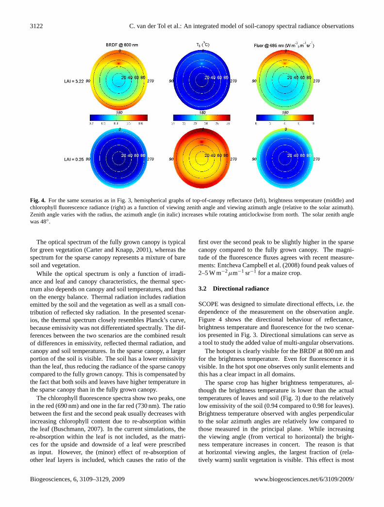
Fig. 4. For the same scenarios as in Fig. 3, hemispherical graphs of top-of-canopy reflectance (left), brightness temperature (middle) andchlorophyll fluorescence radiance (right) as a function of viewing zenith angle and viewing azimuth angle (relative to the solar azimuth).Zenith angle varies with the radius, the azimuth angle (in italic) increases while rotating anticlockwise from north. The solar zenith anglewas 48◦.
The optical spectrum of the fully grown canopy is typicalfor green vegetation (Carter and Knapp, 2001), whereas thespectrum for the sparse canopy represents a mixture of baresoil and vegetation.
While the optical spectrum is only a function of irradi-ance and leaf and canopy characteristics, the thermal spec-trum also depends on canopy and soil temperatures, and thuson the energy balance. Thermal radiation includes radiationemitted by the soil and the vegetation as well as a small con-tribution of reflected sky radiation. In the presented scenar-ios, the thermal spectrum closely resembles Planck’s curve,because emissivity was not differentiated spectrally. The dif-ferences between the two scenarios are the combined resultof differences in emissivity, reflected thermal radiation, andcanopy and soil temperatures. In the sparse canopy, a largerportion of the soil is visible. The soil has a lower emissivitythan the leaf, thus reducing the radiance of the sparse canopycompared to the fully grown canopy. This is compensated bythe fact that both soils and leaves have higher temperature inthe sparse canopy than in the fully grown canopy.
The chlorophyll fluorescence spectra show two peaks, onein the red (690 nm) and one in the far red (730 nm). The ratiobetween the first and the second peak usually decreases withincreasing chlorophyll content due to re-absorption withinthe leaf (Buschmann, 2007). In the current simulations, there-absorption within the leaf is not included, as the matri-ces for the upside and downside of a leaf were prescribedas input. However, the (minor) effect of re-absorption ofother leaf layers is included, which causes the ratio of the
first over the second peak to be slightly higher in the sparsecanopy compared to the fully grown canopy. The magni-tude of the fluorescence fluxes agrees with recent measure-ments: Entcheva Campbell et al. (2008) found peak values of2–5 W m−2µm−1 sr−1 for a maize crop.
3.2 Directional radiance
SCOPE was designed to simulate directional effects, i.e. thedependence of the measurement on the observation angle.Figure 4 shows the directional behaviour of reflectance,brightness temperature and fluorescence for the two scenar-ios presented in Fig. 3. Directional simulations can serve asa tool to study the added value of multi-angular observations.
The hotspot is clearly visible for the BRDF at 800 nm andfor the brightness temperature. Even for fluorescence it isvisible. In the hot spot one observes only sunlit elements andthis has a clear impact in all domains.
The sparse crop has higher brightness temperatures, al-though the brightness temperature is lower than the actualtemperatures of leaves and soil (Fig. 3) due to the relativelylow emissivity of the soil (0.94 compared to 0.98 for leaves).Brightness temperature observed with angles perpendicularto the solar azimuth angles are relatively low compared tothose measured in the principal plane. While increasingthe viewing angle (from vertical to horizontal) the bright-ness temperature increases in concert. The reason is thatat horizontal viewing angles, the largest fraction of (rela-tively warm) sunlit vegetation is visible. This effect is most
C. van der Tol et al.: An integrated model of soil-canopy spectral radiance observations 3123
50
1071
Figure 4 1072
20 25 30soil
TOC
T (oC)
LAI = 3.22
dep
th (
LAI)
sunlitshadedaverage
20 25 30
T (oC)
LAI = 0.25
1073
Figure 5 1074 Fig. 5. For the same scenarios as in Fig. 3, vertical profiles of con-tact temperatures of leaves and soil (averages per layer). The topof the graph represents the top of canopy; the bottom of the graphrepresents the soil. Temperatures are contact (skin) temperatures ofthe canopy, except for the values at the bottom of the graph: theseare contact temperatures of the soil. The vertical axis scales linearlywith leaf area index.
pronounced in the sparse vegetation, because there the differ-ences in temperature between sunlit and shaded vegetationare the largest (Fig. 5).
The directional effect is quite pronounced for chlorophyllfluorescence. The upper leaves contribute most to totalchlorophyll fluorescence, and as a result, observed fluores-cence increases when moving from vertical to horizontalviewing angles.
Note that clumping of leaves, twigs and branches may alsoaffect the directional effects in forest canopies (Smolanderand Stenberg, 2003). This effect is not included at present,but it may be a feature of future versions of the model.
3.3 Vertical profiles
One of the best ways to illustrate the integration of radiativetransfer with the energy balance is by plotting vertical pro-files of the canopy. Figure 5 shows, for the two scenarios ofFig. 3, vertical profiles of leaf and soil surface temperaturein the canopy. Values represent the average per layer, for thesunlit fraction, the shaded fraction, and the weighted averagetemperature. The bottom layer is the soil.
The temperature of both sunlit and shaded leaves in-creases with depth in the canopy (from top to bottom of thegraph), whereas the weighted mean temperature decreaseswith depth, due to the fact that the shaded fraction progres-sively dominates while moving to lower layers. The sparsecanopy has higher leaf temperatures than the fully growncanopy, both for the shaded and the sunlit fraction. This ef-fect is caused by the high net radiation on the soil, result-ing in higher soil contact temperatures, which also affect thecanopy layer above through a higher emittance received frombelow. The weighted average of leaf and soil temperatures isalso higher for the sparse vegetation, because the fraction ofsunlit leaves is higher.
51
-4 -2 0 2soil
TOC
∆ T (oC)
Dep
th
-2 0 2 4 6
∆ A (µmol m-2s-1)-20 0 20 40
∆ λE (W m-2) 1075
Figure 6 1076
0.4 0.6 0.8 1 1.2 1.4 1.60
0.1
0.2
0.3
0.4
0.5
Wavelength (µm)
Ref
lect
ance
A prioriCalibratedMeasured
1077
Figure 7 1078
Fig. 6. The effect of increasing wind speed from 2.9 m s−1 to15 m s−1 (blue line and triangles), and the effect of replacing alldirect radiation by diffuse radiation -while total radiation remainsunchanged- (green line with circles), for the fully grown maizecanopy of Fig. 3. The graphs show the difference in the verticalprofiles of leaf and soil temperatures, net photosynthesis and latentheat flux compared to the reference scenario.
The vertical profiles are sensitive to variations in irradi-ance regime as well as weather conditions. Different ver-tical profiles of the fully grown maize field resulted by (1)a fivefold higher wind speed (15 m s−1), and (2) replacingall direct radiation by diffuse radiation (Fig. 6). Not onlythe vertical profiles of temperature change, but also those ofphotosynthesis and latent heat.
Wind speed has a significant effect on temperature, butonly minor effect on the fluxes: the decrease in aerodynamicresistances as wind speed increases is counterbalanced by asimultaneous decrease in the vapour and carbon dioxide gra-dients. The distribution of radiation over direct and diffuseradiation has a significant effect on both the temperature andthe fluxes. This results confirms that photosynthetic light useefficiency is higher for diffuse than for direct radiation (Guet al., 2002).
4 Applications of SCOPE
In this section, a number of simulations are presented to ad-dress the potential and the limitations of the SCOPE model.Most of the individual components of the model have beenvalidated before, such as the optical radiative transfer model(Jacquemoud et al., 2000) and the leaf physiological model(Von Caemmerer and Baker, 2007). A validation of all com-ponents of the model against field data will be the topic of afollow-up paper.
4.1 Plant physiology
SCOPE has potential applications for plant physiology andcarbon uptake. This is illustrated in Fig. 7, showing mea-sured (with an ASD radiometer) and simulated reflectancespectra of a Pine forest in The Netherlands. Data were
3124 C. van der Tol et al.: An integrated model of soil-canopy spectral radiance observations
51
-4 -2 0 2soil
TOC
∆ T (oC)
Dep
th
-2 0 2 4 6
∆ A (µmol m-2s-1)
-20 0 20 40
∆ λE (W m-2) 1075
Figure 6 1076
0.4 0.6 0.8 1 1.2 1.4 1.60
0.1
0.2
0.3
0.4
0.5
Wavelength (µm)
Ref
lect
ance
A prioriCalibratedMeasured
1077
Figure 7 1078 Fig. 7. Measured and simulated spectrum of radiance ver-sus wavelength for a Pine forest in The Netherlands, 13 June2006 at 11:45 local (winter) time (GMT+1). Measurements weretaken with an ASD spectrometer from a 46 m tower raising 16 mabove the canopy (solar zenith angleθs=30.6◦, solar azimuth an-gle φs=345◦, observer zenith angleθo=30◦, observer azimuthangle φo=185◦). A priori parameter values of Table 2 wereused. Calibration was carried out using a non-linear least squaressolver. Calibrated PROSPECT parameters were:Cab=47µg cm−2,Cdm=0.025 g cm−2, Cw=0.0195 cm,Cs=0.114,N=1.07.
collected during an intensive field campaign (EAGLE) inJune 2006, described in detail by Su et al. (2009). Simula-tions were carried out both using a priori, literature values forthe PROSPECT parameters (Table 2), and using calibratedPROSPECT parameters (calibration of SCOPE was carriedout using a non-linear least square solver). Fitting the modelto observations resulted in PROSPECT parameter values forchlorophyll content and leaf water content that were differentfrom the a priori values. Although currently no model existsto relate PROSPECT parameters to plant physiological pro-cesses such as photosynthesis, it is theoretically possible tolimit the parameter space of SCOPE by linking calibratedoptical parameters of PROSPECT to parameters of the bio-chemical leaf model. Such approach would greatly improvethe remote sensing of physiology and carbon uptake.
4.2 Testing of surface energy balance models
A different application is to use SCOPE to evaluate and im-prove simpler, operational remote sensing based surface en-ergy balance models, such as SEBAL (Bastiaanssen, 1998)or SEBS (Su, 2002). The use of SCOPE as a hypotheti-cal ground truth not only provides the necessary validationdata, but also simulates the input data, notably the TOC ra-diative spectra. By using these simulated spectra, complica-
tions due to differences in scale between ground and remotesensing images and issues of atmospheric correction are cir-cumvented.
An example is given in Fig. 8. This figure shows onthe left, simulated input, and on the right, simulated outputfor the model SEBS. The left graphs shows the differencebetween brightness temperature (calculated from outgoinglong wave radiance), and air temperature measured abovethe canopy. The input data for this simulation were collectedduring a field experiment in Barrax (Spain) on 17 July 2004(Su et al., 2008). Field measurements for validation are alsoshown in the graph. Brightness temperature is the most im-portant input variable of SEBS, but other variables such asNDVI can be simulated with SCOPE as well.
4.3 Interpolation between satellite overpasses
A related possible application of SCOPE is to interpolatefluxes between satellite overpasses. The model can run inthe absence of remote sensing information, which makes itpossible to not only scale from instantaneous data to diurnalcycles, but also to calculate the fluxes for clouded days, forwhich reliable remote sensing data are not available.
4.4 The use of chlorophyll fluorescence
The use of chlorophyll fluorescence signal is another promis-ing application. The SCOPE model contains parameterswhich control the amount of fluorescence per leaf as a func-tion of leaf physiological parameters likeVc,max andλ, theoptical parameters of the PROSPECT model, such as thechlorophyll content, and light and temperature conditions in-side the canopy. Since leaf photosynthesis is included in themodelling as well, one could investigate the relationships be-tween light use efficiency and fluorescence at the canopylevel under different simulated conditions (stress, canopystructure, weather, etc.). This could be of great help for thecorrect interpretation of fluorescence measurements from asatellite mission like FLEX (Rascher et al., 2008).
5 Conclusions
SCOPE integrates radiative transfer and energy balance cal-culations at the level of individual leaves as well as thecanopy. Potential applications are in plant physiology, re-mote sensing of the energy balance, and the preparation offuture satellite missions such as the fluorescence explorermission FLEX. The modular structure of SCOPE makes itpossible to add new features by simply sharing input, out-put and parameters with other models. Future developmentsinclude the adding a library of MODTRAN output spectrafor various weather conditions, as well as a library of soilspectra.
C. van der Tol et al.: An integrated model of soil-canopy spectral radiance observations 3125
52
0 6 12 18 24-4
-2
0
2
4
6
8
10
12
time (hours)
Tb-T
a (o C
)
0 6 12 18 24-100
0
100
200
300
400
500
time (hours)
λE (
W m
-2)
Tb mod
-Ta
Tb meas
-Ta
λEmod
Hmod
λEmeas
Hmeas
1079
Figure 8 1080 Fig. 8. Measured and simulated diurnal cycles of brightness temperature, latent and sensible heat flux for a Vineyard in Barrax, Spain,17 July 2004. Measured brightness temperature was based on measurements of a radiometer above the canopy, latent and sensible heat fluxon measurements with a sonic anemometer and open path gas analyser.
Appendix A
Numerically stable fluxes in the 4SAIL model
The two-stream radiative transfer equation in matrix-vectorform reads
d
Ldx
(E−
E+
)=
(a −σ
σ −a
)(E−
E+
). (A1)
With the eigenvaluem=√(a−σ)(a+σ), one can de-
fine the so-called infinite reflectance, which is given byr∞=
a−mσ
, and by means of the left-hand eigenvector matrix(1 −r∞
−r∞ 1
)one can define transformed fluxes given by(
F1F2
)=
(1 −r∞
−r∞ 1
)(E−
E+
). (A2)
This transformation establishes the diagonalization of thetwo-stream radiative transfer matrix, since
d
Ldx
(F1F2
)=
(1 −r∞
−r∞ 1
)(a −σ
σ −a
)(E−
E+
)
=
(m 00 −m
)(1 −r∞
−r∞ 1
)(E−
E+
)
=
(m 00 −m
)(F1F2
). (A3)
Addition of direct solar flux and thermal emittance by thefoliage to Eq. (A1) gives
d
Ldx
(E−
E+
)= Es(0)e
kLx
(−s′
s
)+
(a −σ
σ −a
)(E−
E+
)
+ εv
(−HcHc
). (A4)
The transformation by the left-hand eigenvector matrix cannow be applied again to obtain
d
Ldx
(F1F2
)= Es(0)e
kLx
(−s′ −r∞s
r∞s′+s
)+
(m 00 −m
)(F1F2
)
+ εv(1+r∞)
(−HcHc
). (A5)
One can write
1+r∞
1−r∞=
1+a−mσ
1−a−mσ
=σ +a−m
σ −a+m=m(a+σ −m)
m2−m(a−σ)
=m(a+σ −m)
(a−σ)(a+σ −m)=
m
a−σ. (A6)
Sincea−σ=α=εc (Kirchhoff’s law), whereα is the ab-sorption coefficient andεc the foliage emissivity, one canwrite (1+r∞)εc=m(1−r∞), so finally the following differ-ential equations are obtained:
d
LdxF1 = mF1−(s′ +r∞s)Es−m(1−r∞)Hc
d
LdxF2 = −mF2+
(r∞s
′+s)Es+m(1−r∞)Hc . (A7)
Numerically stable analytical solutions of these differentialequations are given by
3126 C. van der Tol et al.: An integrated model of soil-canopy spectral radiance observations
+ (1−r∞)Hc , (A8)
whereδ1 andδ2 are constants which have to be determinedfrom the boundary equations.
Defining the functions
J1(q,x) =emLx−eqLx
q−m
J2(q,x) =eqL(1+x)
−e−mL(1+x)
q+me−qL , (A9)
one can write
F1 = δ1emLx
+(s′ +r∞s)Es(0)J1(k,x)+(1−r∞)Hc
F2 = δ2e−mL(1+x)
+(r∞s′+s)Es(0)J2(k,x)
+ (1−r∞)Hc . (A10)
FunctionJ2(q,x) is numerically stable, butJ1(q,x) mustbe approximated by a different function ifq-m is small, sayless than 10−3. Thus we redefine
J1(q,x)=emLx−eqLx
q−m|q−m| ≥ 10−3
−12
(emLx+eqLx
)Lx[
1−112(q−m)2L2x2
]|q−m|<10−3
. (A11)
The energy balance, and therefore also leaf temperatures,photosynthesis and fluorescence, depends on the direct anddiffuse fluxes in the canopy. The direct solar flux followsdirectly from
Es(x)=Es(0)Ps(x),
wherePs(x)=exp(kLx) is the probability of sunshine (or thegap fraction in the direction of the sun),L is the total LAIandx the relative optical height, which runs from−1 at thebottom to zero at the canopy top.
The diffuse fluxes can be calculated once the transformedfluxes have been determined using Eq. (A8). However, thisrequires solving the boundary constantsδ1 andδ2. This canbe achieved by evaluatingF1 at the canopy top, andF2 at thecanopy bottom, giving
F1(0) = δ1+(1−r∞)Hc
F2(−1) = δ2+(1−r∞)Hc . (A12)
Here, use was made of the fact thatJ1(k,0)=0, and alsoJ2(k,−1)=0. In terms of the normal diffuse fluxes one thenobtains
δ1 = F1(0)−(1−r∞)Hc
= E−(0)−r∞E+(0)−(1−r∞)Hc
δ2 = F2(−1)−(1−r∞)Hc
= −r∞E−(−1)+E+(−1)−(1−r∞)Hc . (A13)
If thermal emission is disregarded for the moment, theconstants are given by
δ1 = E−(0)−r∞E+(0)
δ2 = E+(−1)−r∞E−(−1). (A14)
Four-stream radiative transfer for the canopy-soil systemcan now be described by
Es(−1) = τssEs(0)
E−(−1) = τsdEs(0)+τddE−(0)+ρddE
+(−1)
E+(0) = ρsdEs(0)+ρddE−(0)+τddE
+(−1)
E+(−1) = rs[Es(−1)+E−(−1)]. (A15)
Here, the double-subscripted intrinsic reflectance andtransmittance quantities of the isolated canopy layer are pro-vided as output quantities of the 4SAIL model and are givenby
τss = e−kL
τdd =
(1−r2
∞
)e−mL
1−r2∞e
−2mL
ρdd =r∞(1−e−2mL
)1−r2
∞e−2mL
τsd = (s′ +r∞s
)J1(k,−1)−r∞e−mL
(r∞s
′+s)J2(k,0)
1−r2∞e
−2mL
ρsd =
−r∞e−mL
(s′ +r∞s
)J1(k,−1)+(r∞s′ +s)J2(k,0)
1−r2∞e
−2mL.
(A16)
Combining the second and fourth equation of Eq. (A15)gives
E−(−1)−ρddE+(−1) = τsdEs(0)+τddE
−(0)
−rsE−(−1)+E+(−1) = rsEs(−1)= rsτssEs(0). (A17)
SolvingE+(0) from these gives
E+(−1)=(τsd+τss)Es(0)+τddE−(0)
1−rsρddrs . (A18)
In the program FluorSAIL (Miller et al., 2005), a pre-decessor of SCOPE, the following additional equations areused to determine the boundary constants:
C. van der Tol et al.: An integrated model of soil-canopy spectral radiance observations 3127
Note, that onlyEsun=Es(0) and Esky=E−(0) are re-
quired as inputs for these calculations, since all other intrin-sic canopy optical properties are provided by 4SAIL. Calcu-lation of the internal diffuse fluxes in the canopy can nowproceed by using Eq. (A8) and applying the inverse trans-formation toF1 andF2 to obtain back the original diffusefluxes:
F1(x) = δ1emLx
+(s′ +r∞s
)Es(0)J1(k,x)
F2(x) = δ2e−mL(1+x)
+(r∞s
′+s)Es(0)J2(k,x)
E−(x) = [F1(x)+r∞F2(x)]/(1−r2
∞
)E+(x) = [r∞F1(x)+F2(x)]/
(1−r2
∞
). (A20)
Appendix B
Aerodynamic resistance
For aerodynamic resistance, the schematisation of Wallaceand Verhoef (2000) was used. A two-source model was usedwith separate resistances for soil and canopy (Fig. B1).
Aerodynamic resistance in the inertial sublayer is:
rIa =1
Kru∗
[ln
(zr −d
zR−d
)]−9h,v(zr)+9h,v(zR), (B1)
whereKr=0.41 is Von Karman’s constant (the symbolsKan κ are more common in the literature, but these are al-ready reserved for extinction coefficients in this paper),u∗ isthe friction velocity (m s−1), zr the reference height (m),zRheight of the roughness sublayer (m),d is the zero-plane dis-placement (m), and9h,v a stability correction function (seebelow).
The aerodynamic resistance in the roughness sublayer is:
rRa =zR−h
Kru∗(zR−d)−9∗
h,v (zR)+9∗
h,v(h), (B2)
whereh is the vegetation height, and9∗
h,v a stability cor-rection function (see below). Aerodynamic resistance in thecanopy, above the in-canopy source heightz0m+d, is:
rca =hsinh(n)
nKhv(h)
[ln
(en−1
en+1
)− ln
(en(z0m+d)/h−1
en(z0m+d)/h+1
)], (B3)
wherez0m is the roughness height for momentum (m),n awind extinction coefficient (see below), andKhv the eddydiffusivity (see below).
For the boundary layer resistance of leaves:
rcb =70
L
√wl
uz0m, (B4)
wherewl is leaf width (m) anduz0m wind speed atz=z0m+d(see below).
cwr
sbr
scr
cbr
ccr
swr
Ds Dc
D0
Dr
car
Rar
Iar
Fig. B1. Schematic representation of a two-source resistance modelfor resistances to water vapour and heat transport in and above thecanopy, after Wallace and Verhoef (2000). Letter “D” refers to ei-ther temperature (T ) or absolute humidity (q). Other symbols aredefined in Table 1.
The within canopy resistance is:
rcw =
hsinh(n)
nKhv(h1)
[ln
(en(z0m+d)/h−1
en(z0m+d)/h+1
)−ln
(en·0.01/h
−1
en·0.01/h+1
)].
(B5)
Here, the value of 0.01 denotes the roughness length of soil.For the boundary layer resistance of soil and the surface
resistance of vapour transport in soil pores, a priori valuesare used:
rsb = 150sm−1 andrss = 500sm−1 (B6)
The value forrss could be a function of soil moisture content(e.g. Buckley, 2005). For heat transport,rcs=r
ss=0.
In the above equations, friction velocityu∗ (m s−1) is:
u∗ =Kru(z)
[ln
(z−d
z0m
)−9m
(z−d
3
)]−1
, (B7)
where3 Monin-Obukhov length (m). Wind speed at heightz0m+d,uz0, is:
3128 C. van der Tol et al.: An integrated model of soil-canopy spectral radiance observations
Wind extinction coefficientn is calculated as:
n=cdL
2K2r
, (B9)
wherecd (=0.2) is a drag coefficient. The eddy diffusivityKh,v is calculated as:
Kh,v =Kru∗(z−d)8−1m,h,v , (B10)
where z=zr (see Eq. B1) orzR (Eqs. B1 and B2) orh(Eq. B2).
The stability correction functions for neutral conditionsare:
9h,v =9∗
h,v =9m= 0. (B11)
8−1m,h,v = 1. (B12)
In the model, these values are also used for stable conditions(i.e. no stability correction is applied for stable conditions).For unstable conditions:
9h,v = 2log
(1+x2
z
2
). (B13)
9∗
h,v =z−d
zR−d
x2z −1
x2z +1
. (B14)
9m= 2log
(1+xz
2
)+ log
(1+x2
z
2
)−2arctan(xz)+
π
2. (B15)
8−1m,h,v =
(1−16
h−d
3
)1/2. (B16)
In these equations:
xz =
(1−16
z
3
)1/4. (B17)
Acknowledgements.This research was funded by The NetherlandsOrganisation for Scientific Research (NWO), SRON projectnumber EO-071, and partly by the study “Impact assessment ofsolar induced vegetation fluorescence observations from spacefor improving dynamic vegetation models” for the EuropeanSpace Agency under ESTEC Contract No. 20678/07/NL/HE. Theauthors thank Jerome Demarty, Albert Olioso, Federico Magnani,Antonio Volta, Uwe Rascher and Alexander Damm for fruitfuldiscussions and participation in modelling experiments, andJan Elbers, Wim Timmermans, Remco Dost, Li Jia, Zoltan Vekerdyand Kitsiri Weligepolage for fieldwork, data processing andcoordination during the SPARC and EAGLE campaigns. Theauthors also thank the reviewers for thoroughly reading the paperand providing useful suggestions.
Edited by: G. Wohlfahrt
References
Anderson, M. C., Norman, J. M., Kustas, W. P., Houborg, R.,Starks, P. J., and Agam, N.: A thermal-based remote sensingtechnique for routine mapping of land-surface carbon, water andenergy fluxes from field to regional scales, Remote Sens. Envi-ron., 112, 4227–4241, doi:10.1016/j.rse.2008.07.009, 2008.
Baldocchi, D. D.: Assessing the eddy covariance techniquefor evaluating carbon dioxide exchange rates of ecosystems:past, present and future, Glob. Change Biol., 9, 479–492,doi:10.1046/j.1365-2486.2003.00629.x, 2003.
Bastiaanssen, W. G. M., Menenti, M., Feddes, R. A., and Holtslag,A. A. M.: A remote sensing surface energy balance algorithm forland (SEBAL). 1. Formulation, J. Hydrol., 212–213, 198–212,doi:10.1016/S0022-1694(98)00253-4, 1998.
Berk, A., Anderson, G. P., Acharya, P. K., Chetwynd, J. H., Bern-stein, L. S., Shettle, E. P., Matthew, M. W., and Adler-Golden, S.M.: MODTRAN4 USER’S MANUAL, Air Force Research Lab-oratory, Space Vehicles Directorate, Air Force Materiel Com-mand, Hanscom AFB, MA 01731-3010, 97 pp., 2000.
Bhumralkar, C. M.: Numerical Experiments on the Computation ofGround Surface Temperature in an Atmospheric General Circu-lation Model, J. Appl. Meteorol., 14, 1246–1258, 1975.
Buckley, T. N.: The control of stomata by water balance, New Phy-tol., 168, 275–292, 2005
Buschmann, C.: Variability and application of the chlorophyll flu-orescence emission ratio red/far-red of leaves, Photosynth. Res.,92, 261–271, doi:10.1007/s11120-007-9187-8, 2007
Carter, G. A. and Knapp, A. K.: Leaf optical properties in higherplants: linking spectral characteristics to stress and chlorophyllconcentration, Am. J. Bot., 88, 677–684, 2001.
CEOS: The Earth Observation Handbook – Climate change specialedition 2008 (ESA SP-1315), edited by: Bond, P., ESA Commu-nications Production Office, Noordwijk, The Netherlands, 2008.
Collatz, G., Ribas-Carbo, M., and Berry, J. A.: Coupledphotosynthesis-stomatal conductance model for leaves of C4plants, Aus. J. Plant Physiol., 19, 519–538, 1992.
Entcheva Campbell, P. K., Middleton, E. M., Corp, L. A., and Kim,M. S.: Contribution of chlorophyll fluorescence to the appar-ent vegetation reflectance, Sci. Total Environ., 404, 433–439,doi:10.1016/j.scitotenv.2007.11.004, 2008.
Farquhar, G., Von Caemmerer, S., and Berry, J.: A biochemi-cal model of photosynthetic CO2 assimilation in leaves of C3species, Planta, 149, 78–90, 1980.
Genty, B., Birantais, J., and Baker, N.: The relationship betweenthe quantum efficiencies of photosystems I and II in pea leaves,Biochem. Biophys. Acta, 990, 87–92, 1989.
Gu, L., Baldocchi, D., Verma, S. B., Black, T. A., Vesela, T., Falge,E. M., and Dowty, P. R.: Advantages of diffuse radiation for ter-restrial ecosystem productivity, J. Geophys. Res., 107(D6), 4050,doi:10.1029/2001JD001242, 2002.
Guilioni, L., Jones, H. G., Leinonen, I., and Lhomme, J.-P.: Onthe relationships between stomatal resistance and leaf tempera-tures in thermography, Agr. Forest Meteorol., 148, 1908–1912,doi:10.1016/j.agrformet.2008.07.009, 2008.
Hall, F. G., Huemmrich, K. F., Goetz, S. J., Sellers, P. J., and
C. van der Tol et al.: An integrated model of soil-canopy spectral radiance observations 3129
Nickeson, J. E.: Satellite remote sensing of surface energy bal-ance: success, failures, and unresolved issues in FIFE, J. Geo-phys. Res., 97(D17), 19061–19089, 1992.
Houldcroft, C.: Measuring and modeling the surface temperatureand structure of a maize canopy, Ph.D. thesis, The University ofReading, UK, 235 pp., 2004.
Jacquemoud, S. and Baret, F.: PROSPECT: A model of leaf opticalproperties spectra, Remote Sens. Environ., 34, 75–91, 1990.
Jacquemoud, S., Bacour, C., Poilve, H., and Frangi, J.-P.: Compar-ison of four radiative transfer models to simulate plant canopiesreflectance: direct and inverse mode, Remote Sens. Environ., 74,471–481, 2000.
Kull, O. and Kruyt, B.: Acclimation of photosynthesis to light: amechanistic approach, Funct. Ecol., 13(1), 24–36, 1998.
Kustas, W. P., Anderson, M. C., French, A. N., and Vickers, D.:Using a remote sensing field experiment to investigate flux-footprint relations and flux sampling distributions for tower andaircraft-based observations, Adv. Water Resour., 29, 355–368,doi:10.1016/j.advwatres.2005.05.003, 2006.
Kustas, W. P., Anderson, M. C., Norman, J. M., and Li, F.: Utilityof radiometric-aerodynamic temperature relations for heat fluxestimation, Bound.-Lay. Meteorol., 122, 167–187, 2007.
Lloyd, J. and Farquhar, G.: 13C discrimination during CO2 assimi-lation by the terrestrial biosphere, Oecologia, 99, 201–215, 1994.
Makela, A., Hari, P., Berninger, F., Hanninen, H., and Nikinmaa,E.: Acclimation of photosyn-thetic capacity in Scots pine to theannual cycle of temperature, Tree Physiol., 24, 369–376, 2004.
Miller, J., Berger, M., Goulas, Y., Jacquemoud, S., Louis, J.,Mohammed, G., Moise, N., Moreno, J., Moya, I., Pedros,R., Verhoef, W., and Zarco-Tejada, P.: Development ofa Vegetation Fluorescence Canopy Model, ESTEC ContractNo. 16365/02/NL/FF, Final Report, 138 pp., 2005.
Nikolov, N. T., Massman, W. J., and Schoettle, A. W.: Coupling bio-chemical and biophysical processes at the leaf level: an equilib-rium photosynthesis model for leaves of C3 plants, Ecol. Model.,80, 205–235, doi:10.1016/0304-3800(94)00072-P, 1995.
Norman, J. M.: Modeling the complete crop canopy, in: Modifi-cation of the aerial environment of plants, edited by: Barfield,B. J. and Gerber, J. F., ASAE Monogr. Am. Soc. Agric. Engr.,St. Joseph, MI, 249–277, 1979.
Norman, J. N. and Becker, F.: Terminology in thermal infrared re-mote sensing of natural surfaces, Agr. Forest Meteorol., 77, 153–166, doi:10.1016/0168-1923(95)02259-Z, 1995.
Rascher, U., Gioli, B., and Miglietta, F.: FLEX – FluorescenceExplorer: A Remote Sensing Approach to Quantify Spatio-Temporal Variations of Photosynthetic Efficiency from Space,in: “Photosynthesis. Energy from the Sun, 14th InternationalCongress on Photosynthesis”, edited by: Allen, J. F., Gantt, E.,Golbeck, J. H., and Osmond, B., Springer, Netherlands, 2008.
Reich, P. B., Ellsworth, D. S., Walters, M. B., Vose, J. M., Gresham,C., Volin, J. C., and Bowman, W. D.: Generality of leaf traitrelationships: a test across six biomes, Ecology, 80, 1955–1969,1999.
Sellers, P. J., Dickinson, R. E., Randall, D. A., Betts, A., Hall,F., Berry, J., Collatz, G., Denning, A., Mooney, H., Nobre, C.,Sato, N., Field, C., and Henderson-Sellers, A.: Modeling the ex-changes of energy, water, and carbon between continents and theatmosphere, Science, 275(5299), 502–509, 1997.
Smolander, H. and Stenberg, P.: A method to account for shoot scale
Su, Z.: The Surface Energy Balance System (SEBS) for estima-tion of turbulent heat fluxes, Hydrol. Earth Syst. Sci., 6, 85–100,2002,http://www.hydrol-earth-syst-sci.net/6/85/2002/.
Su, Z., Timmermans, W. J., Gieske, A., Jia, L., Elbers, J. A., Olioso,A., Timmermans, J., Van der Velde, R., Jin, X.,Van der Kwast,H., Nerry, F., Sabol, D., Sobrino, J. A., Moreno, J., and Bianchi,R.: Quantification of land-atmosphere exchanges of water, en-ergy and carbon dioxide in space and time over the heteroge-neous Barrax site, Int. J. Remote Sens., 29(17), 5215–5235, 2008.
Su, Z., Timmermans, W. J., van der Tol, C., Dost, R., Bianchi, R.,Gomez, J. A., House, A., Hajnsek, I., Menenti, M., Magliulo, V.,Esposito, M., Haarbrink, R., Bosveld, F., Rothe, R., Baltink, H.K., Vekerdy, Z., Sobrino, J. A., Timmermans, J., van Laake, P.,Salama, S., van der Kwast, H., Claassen, E., Stolk, A., Jia, L.,Moors, E., Hartogensis, O., and Gillespie, A.: EAGLE 2006 -Multi-purpose, multi-angle and multi-sensor in-situ and airbornecampaigns over grassland and forest, Hydrol. Earth Syst. Sci.,13, 833–845, 2009,http://www.hydrol-earth-syst-sci.net/13/833/2009/.
Timmermans, J., Van der Tol, C., Verhoef, W., and Su, Z.: Contactand directional radiative temperature measurements of sunlit andshaded land surface components during the SEN2FLEX 2005campaign, Int. J. Remote Sens., 29(17–18), 5183–5192, 2008.
Tuzet, A., Perrier, A., and Leuning, R.: A coupled model of stom-atal conductance, photo-synthesis and transpiration, Plant CellEnviron., 26, 1097–1116, 2003.
Van der Tol, C., Verhoef, W., and Rosema, A.: A model for chloro-phyll fluorescence and photosynthesis at leaf scale, Agr. ForestMeteorol., 149(1), 96–105, 2009.
Verhoef, W.: Light scattering by leaves with application to canopyreflectance modelling: the SAIL model, Remote Sens. Environ.,16, 125–178, 1984.
Verhoef, W.: Theory of radiative transfer models applied in opticalremote sensing of vegetation canopies, Ph.D. thesis, WageningenAgricultural University, 1998.
Verhoef, A. and Allen, S. J.: A SVAT scheme describing energy andCO2 fluxes for multi-component vegetation: calibration and testfor a Sahelian savannah, Ecol Model., 127, 245–267, 2000.
Verhoef, W. and Bach, H.: Remote sensing data assimilation usingcoupled radiative transfer models, Phys. Chem. Earth Pt. A/B/C,28, 3–13, 2003.
Verhoef, W. and Bach, H.: Coupled soil-leaf-canopy and atmo-sphere radiative transfer modeling to simulate hyperspectralmulti-angular surface reflectance and TOA radiance data, Re-mote Sens. Environ., 109(2), 166–182, 2007.
Verhoef, W., Jia, L., Xiao, Q., and Su, Z.: Unified optical-thermalfour-stream radiative transfer theory for homogeneous vegetationcanopies. IEEE T. Geosci. Remote, 45(6), 1808–1822, 2007.
Von Caemmerer, S. and Baker, N.: The biology of transpiration:from guard cells to globe, Plant Physiol., 143, 3 pp, 2007.
Wallace, J. S. and Verhoef, A.: Modelling interactions in mixed-plant communities: light, water and carbon dioxide, in: LeafDevelopment and Canopy Growth, edited by: Marshall, B. andRoberts, J. A., Sheffield Academic Press, UK, 2000.
Wullschleger, S. D.: Biochemical limitations to carbon assimilationin C3 plants – A retrospective analysis of the A/Ci curves from109 species, J. Exp. Bot., 44, 907–920, 1993.