Procedia Technology 10 ( 2013 ) 381 – 391

2212-0173 © 2013 The Authors. Published by Elsevier Ltd.Selection and peer-review under responsibility of the University of Kalyani, Department of Computer Science & Engineeringdoi: 10.1016/j.protcy.2013.12.374

ScienceDirect

International Conference on Computational Intelligence: Modelling, Techniques and Applications (CIMTA- 2013)

An integrated model with variable production and demand rate under inflation

1S. R. Singh, 2Swati Sharma,*

1,2Department of Mathematics, D. N. College, Meerut 250001, India

Abstract

In this article, an integrated model is developed in which a manufacturer purchases raw materials from a supplier, and then produces finished products/goods, after that delivers them to a buyer. In the intended model production rate is assumed as a function of demand rate and customer demand rate is time dependent. To make the model more realistic the effect of inflation and time value of money is also taken into consideration. The concept of the model is illustrated through the numerical example and sensitivity analysis with respect to the system parameters is also performed. © 2013 The Authors. Published by Elsevier Ltd. Selection and peer-review under responsibility of the University of Kalyani, Department of Computer Science & Engineering.

Keywords: Integrated; inventory model; variable production; time dependent demand rate; inflation

1. Introduction

Computational Intelligence is a collection of methodologies and approaches that deals with complex problems of the real world applications to which traditional methodologies and approaches are fruitless. Computational Intelligence techniques are more convenient for many unusual problems to which long-established techniques are inadequate. Computational techniques play a very significant role in inventory modelling with Supply chain systems.

Supply chain is the coordination and management of the flow of resources within a network of supplier,

* Corresponding author. Tel.: +0-000-000-0000 ; fax: +0-000-000-0000 . E-mail address: jmlashi0@gmail.com.

Available online at www.sciencedirect.com

© 2013 The Authors. Published by Elsevier Ltd.Selection and peer-review under responsibility of the University of Kalyani, Department of Computer Science & Engineering

382 S.R. Singh and Swati Sharma / Procedia Technology 10 ( 2013 ) 381 – 391

manufacturing facility and buyer. In today’s market, competition between individual businesses has shifted to supply lines. Because a synchronized supply chain, can improve service quality through capable information sharing, can produce premium products and can achieve more profit or lower costs. In the last few decades, the supply chain design and management issues have been widely studied. The integrated optimization concept for buyer and vendor was introduced by Goyal [1]. Banerjee [2] developed a model with lot-for-lot policy for the more realistic case of a finite production rate. Goyal [3] relaxed the lot-for-lot policy and invented that the vendor's economic production quantity should be an integer multiple of the buyer's purchase quantity that provided a lower total relevant cost. Banerjee and Kim [4] discussed an integrated just in time inventory model with constant and deterministic demand rate, production rate and delivery time. Later on, Shi and Su [5] suggested an integrated inventory model from the retailer's perception only. Recently, Singh, Singh and Bhatia [6], Singh, Singh [7], Kumar, Singh and Kumari [8] and Omar, Sarker and Othman [9] put forwarded some interesting supply chain models with different but not limited to assumptions.

Moreover, the effects of inflation and time value of money are crucial in practical environment, especially in the developing countries with large scale inflation. Therefore, the effect of inflation and time value of currency/money cannot be ignored in real life situations. To relax the assumption that the inflation does not affect the costs of the inventory system, Buzacott [10] and Misra [11] concurrently developed an economic order quantity (EOQ) model with a constant inflation rate for all allied costs. Bierman and Thomas [12] then proposed an EOQ model under inflation that also incorporated the discount rate. Misra [13] then discussed the EOQ model with different inflation rates for various associated costs. Ray and Chaudhuri [14] developed an inventory model with variable demand, inflation and time discounting. Later on, Yang, Teng and Chern [15] established inventory models with fluctuating demand patterns under inflation. In recent times, Singh, Kumar and Kumari [16], Singh and Swati [17] and Singh, Jain and Pareek [18] all have investigated the effects of inflation in inventory modeling.

Most of the inventory models with supply chain management are developed by considering either infinite or finite but deterministic production rate and do not consider the effect of inflation. Due to, the varying demand and high inflationary surroundings this concept is not convenient. Therefore, in this article an integrated model with variable manufacturing rate and consumption rate is developed incorporating the effect of inflation and time value of money. This paper extends the work of Omar, Sarker and Othman [9] by means of linearly increasing demand, variable production and inflation. The remainder of this paper is organized as follows: Section 2 explains assumptions and notations that are used throughout the study. In Section 3, mathematical models are developed from buyer’s and manufacturer’s point of views and then the integrated supply chain model is constructed. The proposed supply chain model is demonstrated through a numerical example and the sensitivity analysis is carried out in Section 4. Finally, the paper is concluded in Section 5.

2. Assumptions and Nomenclature

In the presented model we have considered a single raw material supplier, a single manufacturer who procures raw material and manufactures the finished product with a variable production rate and delivers the products to a single buyer either at equal replenishment interval or at equal shipment size. The total cost for the integrated system includes the costs of both buyer and manufacturer. To develop the proposed inventory model, we have made the following assumptions and nomenclature.

2.1. Assumptions

1. A single product inventory system is considered over a finite planning horizon. 2. During the production up-time, the finished goods becomes immediately exists to meet up the demand. 3. The demand rate of finished product at any time t during (0, T) is f(t) and assumed to be linearly increasing. 4. Shortages are not allowed. 5. The production rate is P= f(t) where > 1 for all t. 6. Only one type of raw material is considered.

383 S.R. Singh and Swati Sharma / Procedia Technology 10 ( 2013 ) 381 – 391

Fig. 1: Buyer’s inventory system for equal lots shipments size q.

Nomenclature

Cp is the manufacturing set-up cost. C1 is the ordering cost for raw material. Cb is the shipment cost Hp is the inventory carrying cost per unit per unit time for finished product at the manufacturer end. H1 is the inventory carrying cost per unit per unit time for raw material. Hb is the inventory carrying cost per unit per unit time at the buyer’s side. d is the discount rate. i is the inflation rate. r(=d-i) is the discount rate minus the inflation rate. n is the number of shipment from manufacturer to the buyer. m is the number of raw material batches from supplier to the manufacturer.

3. Mathematical Formulation and Solution

3.1. Buyer’s inventory system

The buyer’s inventory system is depicted in Fig. 1. It is considered that there are ‘n’ cycles at the buyer’s part during the time period [0, T] and either time for each shipment is same or the lot size for each shipment is same. X is the amount of inventory which is needed by the buyer at the beginning of a production cycle to meet the customer demand that also provides the manufacturer enough time to build up inventory for upcoming deliveries. When these X units are utilized completely, the buyer gets the first shipment from the manufacturer. In every batch, due to the customer’s demand buyer’s inventory reduces up to zero. The stock level during any period [ti, ti+1], where i=0, 1, 2,… n-1 is given by the following differential equation:

I '( t ) f ( t )= − ti t ti+1 (1)

With boundary condition I(ti) =q. Where, q is the batch size for each shipment and is given by,

i 1

i

t

t

q f ( t ) d t+

= (2)

Integrating eq. (1) from ti to t and using the boundary condition (2), we get

i 1

i

tt

t t

I( t ) q f (u)du f (u )du+

= − = (3)

384 S.R. Singh and Swati Sharma / Procedia Technology 10 ( 2013 ) 381 – 391

The present worth of the shipment cost (OCb) for the buyer for n-shipments is given by

i

n 1rt

b bi 0

O C C e−

−

=

= (4)

The present worth of the holding cost (HCb) for n-shipments for the buyer is given by

( )i 1 i 1

i

i i

t tn 1 n 1r tr t r tb

b bi 0 i 0t t

HH C H I ( t ) e d t f ( t ) e e d t

r

+ +− −−− −

= =

= = −

When demand rate f(t) is (a+bt) then present worth of the holding cost becomes

( ){ } ( ){ }i 1 i

i

2 2 rt rtn 1rtb i 1 i

b i 1 i i 1 i2 2i 0

H bt bt e eHC e at at a bt r b a bt r b

r 2 2 r r

+− −−− +

+ +

=

= + − − + + + − + + (5)

When we consider second policy i.e. the equal shipments lot size where for n-shipments we have

T

0

1q f ( t )d t

n= (6)

It follows that for any shipment cycle

i 1

i

t

t

q f ( t )d t+

= (7)

When demand rate is (a+bt), then from eq. (6) and (7), we have

( )2 2 2i

1 1t a a n 2 a b iT ib T

b n= − + + +

(8)

Now, we calculate present worth of the holding cost (HCbt) for the first policy i.e. when time for each shipment is same. In this case,

it iT n= , so from eq. (5), we get

( )( )

( )

( )

( )

rT2 rT n 2 rT nrT nb

bt 2 2 2 2 rT n rT n

1 ear bH aT bT e bT bT bT eHC a r b e 1

r n n nr2n r r n 1 e 1 e

−− −

−

− −

−+= + − + + + + + −

− −

(9)

Similarly, from eq. (5) the present worth of the holding cost (HCbq) for the second policy i.e. the equal lot size shipment, is given by

( ){ } ( ){ }i 1 i

i

2 2 rt rtn 1rtb i 1 i

bq i 1 i i 1 i2 2i 0

H bt bt e eHC e at at a bt r b a bt r b

r 2 2 r r

+− −−− +

+ +

=

= + − − + + + − + + (10)

Where, ti is given by eq. (8). Therefore, the present worth of the total cost per unit time at buyer’s part (TCBt) for the first policy is given by

385 S.R. Singh and Swati Sharma / Procedia Technology 10 ( 2013 ) 381 – 391

( )

( )

r Tb

t b tr T n

C 1 e1T C B H C

T 1 e

−

−

−= +

−

(11)

Now, the present worth of the total cost per unit time at the buyer’s part (TCBq) for the second policy is given by

i

n 1rt

q b b qi 0

1T C B C e H C

T

−−

=

= + (12)

3.2. Manufacturer’s inventory system

3.2.1. Manufacturer’s Inventory System for finished Goods

Fig. 2 shows the manufacturing inventory level during the period T. Initially, at time t=0 production starts and demand is fulfilled so the inventory level increases during the production period [0, tp] due to the combined effect of the production and demand. The inventory level during the time period [0, tp] for the manufacturer is given by the following differential equation:

( )'1I ( t ) P f ( t ) 1 f ( t )= − = λ − 0 t tp (13)

Fig. 2: Manufacturer’s inventory system (for finished goods) for equal lots shipments size q.

At time tp production process stops and then the inventory level decreases during the period [tp, T] due to the demand of the products. At time t=T inventory becomes zero. The inventory level during the time period [tp, T] is given by the following differential equation:

'2I ( t ) f ( t )= − tp t T (14)

With boundary conditions I1(0)=0 and I2(T)=0. After solving these equations with the help of boundary conditions, we have

( )t

1

0

I ( t ) 1 f ( u ) d u= λ − 0 t tp (15)

T

2t

I ( t ) f (u )d u= tp t T (16)

Now, the total production quantity is equal to the total demand fulfilled during the period [0, T], so we have

pt T

0 0

f ( t )dt f ( t )d tλ = (17)

386 S.R. Singh and Swati Sharma / Procedia Technology 10 ( 2013 ) 381 – 391

After solving eq. (17) we get

( )( )2p

1 1t a a b T 2 a b T

b= − + λ + +

λ

(18)

The quantity X is given by

x

T

t

X f ( t ) d t= (19)

Now, for the first policy, we have

x

T nT

t 0

f ( t )d t f ( t )d tλ = (20)

When f(t)=a+bt then, from eq. (20), we get

( ) ( ){ }2 2 2 2 2x 2

1 1t a a n 2 a b n T n 1 b T n 1

b n= − + λ + λ − + λ −

λ

(21)

For the second policy, we have

x

T T

t 0

1f ( t )d t f ( t )d t

nλ = (22)

When f(t)=a+bt then, from eq. (22), we obtain

( ) ( ){ }2 2 2x

1 1t a a n b T 2 a b T n 1

b n= − + λ + + λ −

λ

(23)

The present worth of the set-up cost (SCm) for the manufacturer is

m pS C C= (24)

Therefore, the present worth of the holding cost (HCm) for the manufacturer is

p

p

tT Trt r t r t

m p 1 2

0 0 t

H C H X e d t I ( t ) e d t I ( t )e d t− − −= + +

( ) ( )( ) ( )

p

p p

x p

rT tT Trt rtrt rt

p

t 0 t

1 e 1 1H f (t )dt f ( t ) e e dt f ( t ) e e dt

r r r

−

− −− −− λ −

= + − + − (25)

When f(t)=a+bt then from eq. (25) the present worth of the holding cost (HCmt) for the first policy is

( )( ) ( )

( ) ( )

( ) ( )

p

p p

rT 2p prt2 2

mt p x x p2 2

22pprt rtrT

p 2 2

1 e a bt bt1b a b bH C H a T t T t e at

r 2 r r r 2r r

a btbt a bT1 bT 1 be aT at e e

r 2 2 r rr r

−

−

− −−

− +λ −= − + − + + − + + +

+++ + − − + + − +

(26)

387 S.R. Singh and Swati Sharma / Procedia Technology 10 ( 2013 ) 381 – 391

Where, tp and tx for the first policy are given by the eq. (18) and (21) respectively. Similarly, the present worth of the holding cost (HCmq) for the second policy is

( )( ) ( )

( ) ( )

( ) ( )

p

p p

rT 2p prt2 2

mq p x x p2 2

22pprt rtrT

p 2 2

1 e a bt bt1b a b bHC H a T t T t e at

r 2 r r r 2r r

a btbt a bT1 bT 1 be aT at e e

r 2 2 r rr r

−

−

− −−

− +λ −= − + − + + − + + +

+++ + − − + + − +

(27)

Where, tp and tx are given by the eq. (18) and (23) respectively.

3.2.2. Manufacturer’s Inventory System for Raw Materials

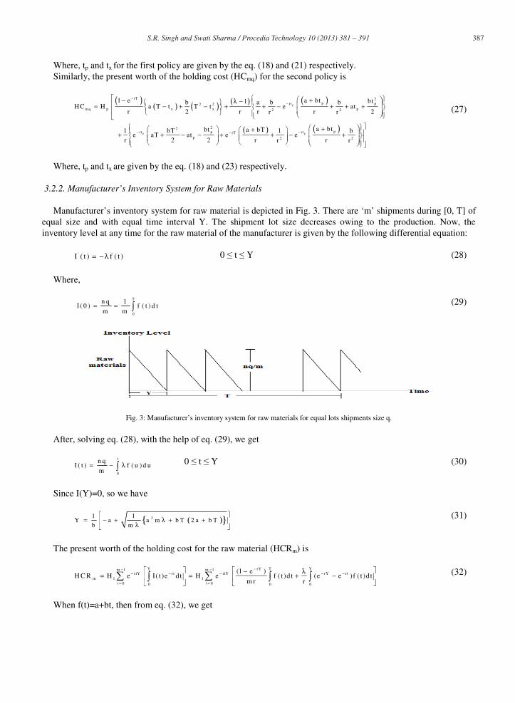
Manufacturer’s inventory system for raw material is depicted in Fig. 3. There are ‘m’ shipments during [0, T] of equal size and with equal time interval Y. The shipment lot size decreases owing to the production. Now, the inventory level at any time for the raw material of the manufacturer is given by the following differential equation:

'I ( t ) f ( t )= − λ 0 t Y (28)

Where,

T

0

n q 1I ( 0 ) f ( t ) d t

m m= =

(29)

Fig. 3: Manufacturer’s inventory system for raw materials for equal lots shipments size q.

After, solving eq. (28), with the help of eq. (29), we get

t

0

n qI ( t ) f ( u ) d u

m= − λ

0 t Y (30)

Since I(Y)=0, so we have

( ){ }21 1Y a a m b T 2 a b T

b m= − + λ + +

λ

(31)

The present worth of the holding cost for the raw material (HCRm) is

Y T YrYm 1 m 1riY rt riY rY rt

m 1 1i 0 i 00 0 0

(1 e )H C R H e I( t )e dt H e f ( t )d t (e e )f ( t )d t

m r r

−− −− − − − −

= =

− λ= = + −

(32)

When f(t)=a+bt, then from eq. (32), we get

388 S.R. Singh and Swati Sharma / Procedia Technology 10 ( 2013 ) 381 – 391

( )

( )

rmYrY 2 2rY rY

m 1 2 2 rY

1 e(1 e ) (a bY )bT bT b a bHCR H aT aT e e

mr 2 r 2 r rr r 1 e

−−

− −

−

−− +λ= + + + + + − −

−

(33)

The present worth of the ordering cost for raw material (OCRm) is

( ) ( )m 1

riY rmY rYm 1 1

i 0

OCR C e C 1 e 1 e−

− − −

=

= = − − (34)

The present worth of the total cost per unit time for the raw material (TCRm) is

[ ]m m m

1T C R O C R H C R

T= + (35)

Now, the present worth of the total cost per unit time (TCMt) for the manufacturer when the first policy is considered, is

[ ]t m m t m

1T C M S C H C T C R

T= + + (36)

Similarly, the present worth of the total cost per unit time (TCMq) for the manufacturer when the second policy is considered, is

q m m q m

1T C M S C H C T C R

T= + + (37)

The present worth of the total cost per unit time (TCt) for the system when the first policy (when time for each shipment is same) is assumed, is

t t tT C T C M T C B= + (38)

Again, the present worth of the total cost per unit time (TCq) for the system when the second policy (the equal lot size shipment policy) is deliberated, is

q q qT C T C M T C B= + (39)

4. Numerical Example and Sensitivity Analysis

Let us consider a numerical example with the following data (Omar, Sarker and Othman [9]): a=7000, b=700, Cp=200, C1=80, Cb=30, Hp=5, H1=3 and Hb=8 including =1.5, r=0.09 and f (t)=a+bt.

The best solution for policy 1 is m=2, n=10, T=0.194106 TCt=6791.79 and for policy 2 is m=2, n=8, T=0.194626, TCq=6145.17, it is revealed with the help of Table 1. The total associated costs per unit time for the system, for equal lots shipment size policy are given in parentheses in Table 1. The total production quantity for policy 1 is 1371.93 and for policy 2, is 1375.64. Computational techniques are so much helpful in modelling and analyze a practical problem. In this paper, all the calculations are done with the help of software MATHEMATICA 8.0. Fig. 4 provides the behavior of the costs functions for policies 1 and 2 regarding n. Sensitivity analysis is also executed through the Tables 2-7.

Table 1: Minimum total costs, TCt and TCq for different arrangement of m and n.

m N

5 6 7 8 9 10 11 12 13 14 15

389 S.R. Singh and Swati Sharma / Procedia Technology 10 ( 2013 ) 381 – 391

Table 2: Effect of parameter Cp on m, n, TCt and TCq.

Fig. 4: Behavior of the cost functions when m=2 against n for both policies

Table 3: Effect of parameter C1 on m, n, TCt and TCq.

Table 4: Effect of parameter Cb on m, n, TCt and TCq.

Cb m n(TCt) n(TCq) TCt TCq

15 2 15 12 5877.13 5420.85

30 2 10 8 6791.79 6145.17

45 2 8 7 7495.53 6703.41

Table 5: Effect of parameter Hb on m, n, TCt and TCq.

Hb m n(TCt) n(TCq) TCt TCq

4 2 8 7 6171.22 5780.87

8 2 10 8 6791.79 6145.17

60006200640066006800700072007400

0 5 10 15 20

TC

t and

TC

q

n

TCt

TCq

1 7092.37 6982.80 6935.13 6926.88 6945.02 6981.46 7030.97 7089.98 7156.00 7227.25 7302.41

(6306.38) (6275.99) (6289.17) (6329.41) (6387.29) (6457.01) (6534.87) (6618.38) (6705.83) (6796.01) (6888.06)

2 7241.22 7040.24 6919.56 6846.40 6807.08 6791.79 6794.10 6809.59 6835.13 6868.47 6907.91

(6322.60) (6214.62) (6162.16) (6145.17) (6152.02) (6175.50) (6210.91) (6255.05) (6305.71) (6361.27) (6420.55)

3 7605.39 7347.26 7176.52 7062.91 6988.66 6942.62 6917.43 6908.02 6910.79 6923.12 6943.05

(6591.96) (6435.07) (6342.51) (6291.48) (6268.68) (6265.85) (6277.56) (6300.10) (6330.87) (6367.96) (6409.99)

4 8003.90 7697.84 7488.74 7343.3 7241.93 7172.29 7126.22 7098.11 7083.94 7080.78 7086.44

(6910.13) (6714.69) (6591.02) (6513.97) (6468.82) (6446.4) (6440.64) (6447.42) (6463.81) (6487.67) (6517.43)

Cp m n(TCt) n(TCq) TCt TCq

100 1 6 5 6176.88 5523.05

200 2 10 8 6791.79 6145.17

300 2 12 9 7267.93 6624.07

C1 m n(TCt) n(TCq) TCt TCq

40 3 10 8 6356.6 5709.89

80 2 10 8 6791.79 6145.17

120 2 11 9 7176.54 6531.17

390 S.R. Singh and Swati Sharma / Procedia Technology 10 ( 2013 ) 381 – 391

12 2 12 9 7306.92 6462.20

Table 6: Effect of inflation parameter r on m, n, TCt and TCq.

R m n(TCt) n(TCq) TCt TCq

0.06 2 11 8 7087.72 6157.46

0.09 2 10 8 6791.79 6145.17

0.12 2 10 8 6626.37 6132.88

Table 7: Effect of production parameter on m, n, TCt and TCq.

m n(TCt) n(TCq) TCt TCq

1.5 2 10 8 6791.79 6145.17

2 1 7 6 6983.24 6304.89

2.5 1 7 5 7012.17 6307.32

(1) Sensitivity analysis Tables 2-5 reveal that as the cost parameters Cp, C1, Cb and Hb increase the total cost per unit time for the system increase, the reason is obvious as a cost parameter increases it increases the total associated cost of the system. When Cp and Hb increase the system favors to the larger number of n to reduce the associated cost of the system. When C1 increases the system favors to the smaller number of m to reduce the associated cost of the manufacturer and larger number of n to shrink the holding cost of the buyer. As Cb increases the smaller number of n is favorable for the system. (2) Table 6 reveals that as the inflation parameter r increases the total relevant cost of the system decreases, the reason is that the total cost per unit time is a decreasing function of inflation. In this case, the system is slightly sensitive to n and favors to the smaller number of n. (3) Table 7 shows that as the production parameter increases the total cost per unit time of the system increases. The reason is that more production means more raw-material is required; therefore the total cost of the system increases. In this case, the system is moderately sensitive to m, n and favors to the smaller number of m and n to reduce the total average cost of the system.

5. Conclusion

In this paper, we have developed a mathematical model for coordinating a supply chain inventory system, with variable production and demand rate in inflationary environment. This approach is more realistic ever since it is not appropriate to consider constant production whenever there is a variable demand rate and due to high inflationary surroundings it is matter-of-fact to regard as the system in inflationary environment. In the model presented here, to minimize the holding cost of the system manufacturer must recognize the supply of small quantities of raw material and deliver the products in small lots to the buyer. Computational techniques give a more efficient way to design and analyze a real life problem. It is examined from sensitivity analysis that the model is plenty stable and it is economical to consider the second policy i.e. the equal lots shipment size policy. This approach can also be extended to further problem by considering multiple buyer, manufacturer, supplier and stochastic environment.

Acknowledgement

The second author wish to thank to Council of Scientific and Industrial Research (New Delhi) for providing financial help in the form of JRF vide letter no. 08/017(0017)/2011-EMR-I.

References

[1] Goyal, SK. An integrated inventory model for a single supplier-single customer problem. International Journal of Production Research 1976; 15(1): 107-111. [2] Banerjee A. A joint economic lot size model for purchaser and vendor. Decision Sciences 1986; 17(3): 292–311.

391 S.R. Singh and Swati Sharma / Procedia Technology 10 ( 2013 ) 381 – 391

[3] Goyal SK. A joint economic-lot-size model for purchaser and vendor: A comment. Decision Sciences 1988; 19(1): 236–241. [4] Banerjee A, Kim SL. An integrated JIT inventory model. International Journal of Operations & Production Management 1995; 15(9): 237–244. [5] Shi CS, Su CT. Integrated inventory model of returns-quantity discounts contract. Journal of the Operational Research Society 2004; 55(3): 240–246. [6] Singh SR, Singh AP, Bhatia D. A Supply Chain Model with Variable Holding Cost for Flexible Manufacturing System. International Journal of Operations Research and Optimization 2010; 1(1): 107-120. [7] Singh SR, Singh C. Supply chain model with stochastic lead time under imprecise partially backlogging and fuzzy ramp-type demand for expiring items. International Journal of Operational Research 2010; 8 (4): 511-522. [8] Kumar N, Singh SR, Kumari R. Three Echelon Supply Chain Inventory Model for Deteriorating Items with Limited Storage Facility and Lead-Time under Inflation. International Journal of Services and Operations Management 2012; 13 (1): 98-118. [9] Omar M, Sarker R, Othman WAM. A just-in-time three-level integrated manufacturing system for linearly time-varying demand process. Applied Mathematical Modelling 2013; 37: 1275–1281. [10] Buzacott JA. Economic order quantities with inflation. Operational Research Quarterly 1975; 26 (3): 553–558. [11] Misra RB. A study of inflationary effects on inventory systems. Logistic Spectrum 1975; 9 (3): 260–268. [12] Bierman H, Thomas J. Inventory decisions under inflationary conditions. Decision Sciences 1977; 8(1): 151–155. [13] Misra RB. A note on optimal inventory management under inflation. Naval Research Logistics Quarterly 1979; 26 (1): 161–165. [14] Ray J, Chaudhuri KS. An EOQ model with stock-dependent demand, shortage, inflation and time discounting. International Journal of Production Economics 1997; 53(2): 171–180. [15] Yang HL, Teng JT, Chern MS. Deterministic inventory lot-size models under inflation with shortages and deterioration for fluctuating demand. Naval Research Logistics 2001; 48 (2): 144–158. [16] Singh SR, Kumar N, Kumari R. An inventory model for deteriorating items with shortages and stock-dependent demand under inflation for two-shops under one management. Opsearch (Oct–Dec 2010) 2010; 47(4): 311–329. [17] Singh SR, Swati. An Optimizing Policy for Decaying Items with Ramp-Type Demand and Preservation Technology under Trade Credit and Inflation. Review of Business and Technology Research 2012; 5(1): 54-62. [18] Singh SR, Jain S, Pareek S. An imperfect quality items with learning and inflation under two limited storage capacity. International Journal of Industrial Engineering Computations 2013; 4(4): 479-490.