ORIGINAL RESEARCH Open Access

An integrated multi-energy flow calculationmethod for electricity-gas-thermalintegrated energy systemsMengting Zhu1, Chengsi Xu1, Shufeng Dong1* , Kunjie Tang1 and Chenghong Gu2

Abstract

The modeling and multi-energy flow calculation of an integrated energy system (IES) are the bases of its operationand planning. This paper establishes the models of various energy sub-systems and the coupling equipment for anelectricity-gas-thermal IES, and an integrated multi-energy flow calculation model of the IES is constructed. Asimplified calculation method for the compressor model in a natural gas network, one which is not included in aloop and works in constant compression ratio mode, is also proposed based on the concept of model reduction. Inaddition, a numerical conversion method for dealing with the conflict between nominal value and per unit value inthe multi-energy flow calculation of IES is described. A case study is given to verify the correctness and speed ofthe proposed method, and the electricity-gas-thermal coupling interaction characteristics among sub-systems arestudied.

Keywords: Integrated energy system, Integrated multi-energy flow calculation, Newton-Raphson, Compressor, Perunit value and nominal value

1 IntroductionIn users or building-level systems, through the coordin-ation of heterogenous generation units, energy storagesystems and flexible loads, multiple energies can be sim-ultaneously generated, transmitted, stored and con-sumed. An integrated energy system (IES) is conduciveto the rational planning and optimal operation of variousenergy sources, so as to give full play to the complemen-tary advantages of various energy sources, improve en-ergy efficiency and promote the consumption ofrenewable energy [1–4]. Multi-energy flow calculation,which can determine the operational state of each en-ergy sub-system in an IES for a given network structure,parameters and boundary conditions, is an importantbasis for the planning and optimal operation of IES [5].At present, there are complete energy flow calculationmodels and methods in electricity, gas and thermal

energy sub-systems [6]. The models and methods ofpower flow calculation for transmission and distributionnetworks are introduced in detail in [7, 8], respectively.The flow calculation methods of integrated transmissionand distribution networks have also been widely studied[9, 10]. In [11], steady-state and dynamic energy flowmodels and calculation methods of a natural gas net-work on the basis of thermodynamics and fluid mechan-ics are established. Reference [12] describes the detailedsteady-state hydraulic model and thermal model of athermal network.An IES is a physical entity of the energy internet [13].

With the relative maturity of each energy system model,the modeling and multi-energy flow calculation of anIES including the electricity, natural gas and thermalnetworks or just two of them have been widely studied.At present, the Newton-Raphson method [5, 14–16] ismainly used to solve IES energy flow. This can be di-vided into two solutions, i.e., the integrated solution andthe decomposed solution [17]. In [18], the two solutions

© The Author(s). 2021 Open Access This article is licensed under a Creative Commons Attribution 4.0 International License,which permits use, sharing, adaptation, distribution and reproduction in any medium or format, as long as you giveappropriate credit to the original author(s) and the source, provide a link to the Creative Commons licence, and indicate ifchanges were made. The images or other third party material in this article are included in the article's Creative Commonslicence, unless indicated otherwise in a credit line to the material. If material is not included in the article's Creative Commonslicence and your intended use is not permitted by statutory regulation or exceeds the permitted use, you will need to obtainpermission directly from the copyright holder. To view a copy of this licence, visit http://creativecommons.org/licenses/by/4.0/.

* Correspondence: dongshufeng@zju.edu.cn1College of Electrical and Engineering, Zhejiang University, Zhejiang, ChinaFull list of author information is available at the end of the article

Protection and Control ofModern Power Systems

Zhu et al. Protection and Control of Modern Power Systems (2021) 6:5 https://doi.org/10.1186/s41601-021-00182-2

are used to calculate the energy flow of an electric-thermal coupling system on Barry Island, and it con-cludes that the integrated solution has the advantages offewer iterations and its iterations do not increase withthe size of the system. In [19], an improved practicalmethod is proposed to reduce the complexity caused bythe traditional method in calculating the natural gas sys-tem with compressors, and the integrated calculationmodel of electricity-gas-heat IES is conducted on thisbasis. In [20], a traditional method is used to calculatethe gas system with compressors, and a hybrid techniqueis proposed to solve the energy flow problem of anelectricity-gas system using a genetic algorithm (GA) tosearch the initial values of the gas system. In [21], a newalternate iterative calculation method considering thedifferent characteristics of each system and the scalabil-ity of IES is proposed, and compared with the integratedsolution using an example. In [22], a generalized energyflow (GEF) analysis model is proposed and a hybridtechnique combining homotopy and the Newton-Raphson algorithm is used to solve the nonlinear equa-tions of GEF.Although there has been some progress in the model-

ing and multi-energy flow calculation of an IES, somechallenges remain. First, users or building level IES usu-ally include electricity, gas, and heat / cold energy. Whilethere are many studies on an electricity-thermal coup-ling or electricity-gas coupling energy system, few stud-ies consider electricity-gas-thermal energy coupling.Second, in the multi-energy flow calculation of an IES,there are many forms of energy. The use of per unitvalue in a power system has many advantages, whileother energy systems usually use nominal values. How-ever, there are no clear steps for data processing to solvethis problem. Third, there are few studies on the energyflow calculation of a natural gas pipeline model with acompressor.When considering users or building level IES, there

are also some special requirements. First, the co-existence of electricity, gas, and heat / cold energymeans the energy sub-systems are closely coupled. Sec-ond, it includes a variety of equipment, and thus thetype of models needs to be determined according to spe-cific requirements. For example, when considering theuncertainty of distributed energy output [23, 24] and thevolatility of load, it is necessary to establish a dynamic orprobabilistic multi-energy flow calculation model.For an IES including electricity, gas supply and heating

networks, this paper makes the following maincontributions:

i. Establishes the steady-state models of electricity,heat, natural gas sub-systems and the couplingequipment. The integrated multi-energy flow

calculation model and method are presented withthe calculation steps given in detail.

ii. Based on the reduction concept, a simplifiedcalculation method is proposed for a compressorwhich is not included in any loop and whoseworking mode is constant compression ratio.

iii. Proposes a simple and fast numerical conversionmethod to deal with the conflicts caused by the useof per unit value in power system and nominalvalue in thermal and natural gas systems in theprocess of the integrated multi-energy flowcalculation.

iv. Studies the coupling interaction characteristics ofthe electricity-gas-thermal IES considering thesource-load characteristics.

The rest of the paper is organized as follows. Section 2presents the models of electricity, district heat and nat-ural gas systems, and proposes a simplified calculationmethod for a natural gas network model with compres-sor. In Section 3, the integrated multi-energy flow calcu-lation model and method are illustrated. In Section 4, acase study is given to verify the correctness and speed ofthe proposed method, and the coupling interactionamong sub-systems is studied. Finally, Section 5 drawsthe conclusion.

2 Model of the electricity-gas-thermal IES2.1 Electricity system modelThis paper uses the AC power flow model, in which thenode voltage is expressed in the form of polar coordi-nates. The node power expressions are given as:

Pi ¼ V i

Xnj¼1

V j Gij cosθij þ Bij sinθij� � ð1Þ

Qi ¼ V i

Xnj¼1

V j Gij sinθij − Bij cosθij� � ð2Þ

where Pi and Qi represent the active power and reactivepower of node i, respectively. Vi and Vj represent thevoltage of node i and j, respectively, while Gij and Bij

represent the conductance and admittance betweennode i and j, respectively. n is the number of nodes andθij is the phase angle between node i and j.

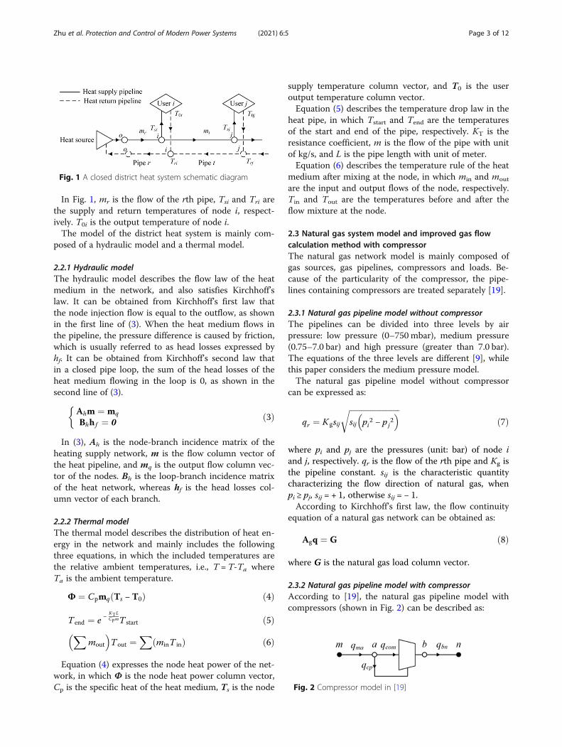
2.2 District heat system modelFigure 1 shows a closed district heat system, which ismainly composed of heat sources, supply pipelines, re-turn pipelines and heat loads. In the network, the heatmedium (usually hot water or steam) transports heatfrom the heat source to the users through the supplypipelines and then flows back to the heat source throughthe return pipelines.

Zhu et al. Protection and Control of Modern Power Systems (2021) 6:5 Page 2 of 12

In Fig. 1, mr is the flow of the rth pipe, Tsi and Tri arethe supply and return temperatures of node i, respect-ively. T0i is the output temperature of node i.The model of the district heat system is mainly com-

posed of a hydraulic model and a thermal model.

2.2.1 Hydraulic modelThe hydraulic model describes the flow law of the heatmedium in the network, and also satisfies Kirchhoff’slaw. It can be obtained from Kirchhoff’s first law thatthe node injection flow is equal to the outflow, as shownin the first line of (3). When the heat medium flows inthe pipeline, the pressure difference is caused by friction,which is usually referred to as head losses expressed byhf. It can be obtained from Kirchhoff’s second law thatin a closed pipe loop, the sum of the head losses of theheat medium flowing in the loop is 0, as shown in thesecond line of (3).

Ahm ¼ mq

Bhh f ¼ 0

�ð3Þ

In (3), Ah is the node-branch incidence matrix of theheating supply network, m is the flow column vector ofthe heat pipeline, and mq is the output flow column vec-tor of the nodes. Bh is the loop-branch incidence matrixof the heat network, whereas hf is the head losses col-umn vector of each branch.

2.2.2 Thermal modelThe thermal model describes the distribution of heat en-ergy in the network and mainly includes the followingthree equations, in which the included temperatures arethe relative ambient temperatures, i.e., T = T-Ta whereTa is the ambient temperature.

Φ ¼ Cpmq Ts − T0ð Þ ð4Þ

T end ¼ e −KTLCpmT start ð5Þ

Xmout

� �Tout ¼

XminT inð Þ ð6Þ

Equation (4) expresses the node heat power of the net-work, in which Φ is the node heat power column vector,Cp is the specific heat of the heat medium, Ts is the node

supply temperature column vector, and T0 is the useroutput temperature column vector.Equation (5) describes the temperature drop law in the

heat pipe, in which Tstart and Tend are the temperaturesof the start and end of the pipe, respectively. KT is theresistance coefficient, m is the flow of the pipe with unitof kg/s, and L is the pipe length with unit of meter.Equation (6) describes the temperature rule of the heat

medium after mixing at the node, in which min and mout

are the input and output flows of the node, respectively.Tin and Tout are the temperatures before and after theflow mixture at the node.

2.3 Natural gas system model and improved gas flowcalculation method with compressorThe natural gas network model is mainly composed ofgas sources, gas pipelines, compressors and loads. Be-cause of the particularity of the compressor, the pipe-lines containing compressors are treated separately [19].

2.3.1 Natural gas pipeline model without compressorThe pipelines can be divided into three levels by airpressure: low pressure (0–750 mbar), medium pressure(0.75–7.0 bar) and high pressure (greater than 7.0 bar).The equations of the three levels are different [9], whilethis paper considers the medium pressure model.The natural gas pipeline model without compressor

can be expressed as:

qr ¼ K gsij

ffiffiffiffiffiffiffiffiffiffiffiffiffiffiffiffiffiffiffiffiffiffiffiffiffiffisij pi2 − pj

2� �r

ð7Þ

where pi and pj are the pressures (unit: bar) of node iand j, respectively. qr is the flow of the rth pipe and Kg isthe pipeline constant. sij is the characteristic quantitycharacterizing the flow direction of natural gas, whenpi ≥ pj, sij = + 1, otherwise sij = − 1.According to Kirchhoff’s first law, the flow continuity

equation of a natural gas network can be obtained as:

Agq ¼ G ð8Þ

where G is the natural gas load column vector.

2.3.2 Natural gas pipeline model with compressorAccording to [19], the natural gas pipeline model withcompressors (shown in Fig. 2) can be described as:

Fig. 1 A closed district heat system schematic diagram

Fig. 2 Compressor model in [19]

Zhu et al. Protection and Control of Modern Power Systems (2021) 6:5 Page 3 of 12

qcom ¼ qbn ¼ K gbn

ffiffiffiffiffiffiffiffiffiffiffiffiffiffiffiffiffiffipb2 − pn2

pqcp ¼

kcpqcomT gas

qgaskcp

s − 1s − 1

� �qma ¼ qcom þ qcp

qma ¼ K gma

ffiffiffiffiffiffiffiffiffiffiffiffiffiffiffiffiffiffiffipm2 − pa2

p

8>>>>><>>>>>:

ð9Þ

where qcom is gas flow through the compressor, and qma

and qbn are the input and output flows of the compres-sor, respectively. qcp is the natural gas consumption ofthe compressor, kcp is the compression ratio, and kcp =pb/pa. Kgma and Kgbn are the pipeline constants of pipesma and bn, respectively. Tgas is the gas temperature inthe pipe, qgas is the calorific value of natural gas, and s isa polytropic index.As shown in Fig. 2, in this paper, m, a, b and n are set

as the nodes in the natural gas network, while nodes aand b are the entry and exit nodes of the compressor, re-spectively. The compressor is located on the pipeline ab.Based on this, the natural gas network model of thecompressor is divided into two categories. One is themodel in which the compressor is included in a loop,as shown in Fig. 3, and the other is the model inwhich the compressor is not included in a loop, asshown in Fig. 4.For the compressor included in a natural gas pipeline

loop, because the nodes on both sides of the compressorare connected to each other, the method proposed in[19] is used to calculate the compressor flow. The spe-cific calculation process is shown in Fig. 5. Based on thedifferent control modes of the compressor, it calculatesthe input and output flows of the compressor, and con-verts them into the equivalent load of the entry and exitnodes of the compressor, respectively. In the later calcu-lation of gas network energy flow, the pipeline contain-ing compressor is viewed as being cut off.For a compressor which is not included in a natural

gas pipeline loop, and works in the mode of a constantcompression ratio, this paper proposes a method similarto the voltage level reduction method of a power systemtransformer to simplify the calculation.As shown in Fig. 6, the known compression ratio of

the compressor kcp1 reduces the pressure of the high-pressure side to the low side of the compressor. Therelevant node pressure changes are:

pb ¼ pa; p0n ¼pnkcp1

; p0s ¼pskcp1

; ð10Þ

According to (10) and from (7) and (8), it can be con-cluded that the pipe flow and the node gas load also re-quire a corresponding operation as:

q0bn ¼ qbnkcp1

; q0ns ¼qnskcp1

ð11Þ

G0n ¼

Gn

kcp1; G0

s ¼Gs

kcp1ð12Þ

As shown in Fig. 7, the reduced compressor can beequivalent to node o, and its gas load is qcp’ = qcp∕kcp1.However, the model of the compressor is nonlinear andchanges need to be made in order to make its flow con-tinuous. Before calculating the deviation, for the elementof the node-branch incidence matrix whose row is corre-sponding to equivalent node o, the column correspond-ing to the next pipeline on, should multiply kcp1, i.e.,qma = kcp1∙qbn’ +Go = qbn + qcp∕kcp1. In addition, the errorcaused by the reduction of natural gas consumption bythe compressor, i.e. (kcp1–1)qcp∕ kcp1, can be ignored as itis relatively small.Using the reduced parameters for subsequent calcula-

tion, this method needs to multiply the parameters ofthe corresponding nodes by kcp1 after calculation. Whenthere are multiple compressors, it is similar to multivoltage levels of the power system, and the method isunchanged, and is repeated here.By using the proposed reduction method, the com-

pressor working in the mode of constant compressionratio does not need to go through the iterative calcula-tion proposed in [19]. This can simplify the calculationsteps and reduce the calculation time.The reliability of the improved method is proved by an

example in Section 4.1.

2.4 Coupling equipment modelIn an IES, the energy sub-systems are closely connectedby coupling equipment. Common multi-energy couplingequipment includes combined heat and power (CHP)systems, gas turbines, electric boilers, etc. In this paper,the most common CHP system [25, 26] is considered asthe coupling equipment.Fig. 3 Compressor located in a loop

Fig. 4 Compressor not located in a loop

Zhu et al. Protection and Control of Modern Power Systems (2021) 6:5 Page 4 of 12

The CHP system with natural gas as input fuel is con-sidered to operate in the following thermal load (FTL)mode. Using the method proposed by the Public UtilitiesRegulatory Policies Act of 1978 [27] to calculate the effi-ciency of the CHP system, the relationship among elec-tric power PCHP, thermal power ΦCHP and natural gasconsumption Gin can be obtained as follows:

PCHP ¼ ΦCHP

cCHP

Gin ¼PCHP þ ΦCHP

2ηCHP

8>>><>>>:

ð13Þ

where cCHP is the power-to-heat ratio of the CHP systemand ηCHP is the efficiency of the CHP system.

3 The integrated calculation method and dataprocessing3.1 Integrated calculation model of IESAccording to [19], the integrated multi-energy flow calcu-lation model of the electricity-gas-thermal IES is given as:

F xð Þ ¼

ΔPΔQΔΦΔh f

ΔTsΔTrΔG

0BBBBBB@

1CCCCCCA

¼

Re V̇ YV̇ð Þn o

− PL ¼ 0

Im V̇ YV̇ð Þn o

−QL ¼ 0

CpAh1m Ts − T0ð Þ −ΦL ¼ 0BhKhm mj j ¼ 0CsTsload − bs ¼ 0CrTrload − br ¼ 0

Ag1Kg −AgTΠ

� �−GL ¼ 0

0BBBBBBBBBB@

1CCCCCCCCCCA

ð14Þ

In (14), rows 1–2 are the power balance equations ofthe electricity system, rows 3–6 are the balance equa-tions of the thermal system, and row 7 is the natural gasflow balance equation. ΔP and ΔQ are the deviations ofFig. 6 Example of compressor not included in loop [19]

Fig. 5 Flow chart for calculating pipeline flow with compressor used in [19]

Zhu et al. Protection and Control of Modern Power Systems (2021) 6:5 Page 5 of 12

the active and reactive power of the electrical power sys-tem, respectively. ΔΦ, Δhf, ΔTs and ΔTr represent thedeviations of the nodal heat power, the loop head losses,the supply and return temperatures, respectively. ΔGrepresents the nodal flow deviation of the natural gassystem. PL, QL, ΦL and GL are the given active power,reactive power, heat power and natural gas load, respect-ively. Ah1 is the node-branch incidence matrix of theheating network, which has removed the heat sourcenodes. Cs, Cr, bs and br are the matrices related to thepipe flow and the output temperature of the thermalnetwork, and their specific calculations can be referredto [12]. Ag is the node-branch incidence matrix of thenatural gas system while Ag1 is derived from Ag by re-moving the gas source node and compressor branch. Πrepresents p2 which is the column vector of the squareof node pressure in a natural gas network, while -Ag

TΠrepresents the square difference vector of a natural gasnetwork. x = [V, θ, m, Tsload, Trload, Π]T are the statevariables of the IES calculation.

3.2 Data processing of the IES Jacobian matrixUsing the extended Newton-Raphson method to calcu-late the electricity-gas-thermal IES system, the IESJacobian matrix can be noted as:

J ¼Jee Jeh JegJhe Jhh JhgJge Jgh Jgg

0@

1A

¼

∂ΔFe

∂xe

∂ΔFe∂xh

∂ΔFe∂xg

∂ΔFh

∂xe

∂ΔFh∂xh

∂ΔFh∂xg

∂ΔFg∂xe

∂ΔFg

∂xh

∂ΔFg∂xg

0BBBBBB@

1CCCCCCA

ð15Þ

where Jee, Jhh and Jgg are the matrices on the diagonalblock, which can be derived independently from eachenergy sub-system. The expressions of Jhh and Jgg aregiven in Section 6.1 and 6.2.Considering the electricity sub-system in an IES is

connected to the bulk power grid, when an internal fluc-tuation occurs, it will be balanced by the bulk powergrid, and thus, Jhe and Jge in (15) are zero matrices. Simi-larly, the natural gas system usually contains gas sourcenodes so when an internal fluctuation occurs, it will bebalanced by the gas source. Thus, Jeg and Jhg in (15) arealso zero matrices.

Since the CHP system works in FTL mode, a fluctuationin the thermal network will affect the operational state ofother systems, and thus, Jeh and Jgh are non-zero matrices.The model of CHP system can be expressed as:

ΦCHP;i ¼ CpAhsourcem Ts −T0ð ÞPCHP;i ¼ ΦCHP;i

cCHP

Gin; i ¼PCHP þ ΦCHP

2ηCHP

8>>>>><>>>>>:

ð16Þ

where Ahsource is the row related to the heat source in thenode-branch incidence matrix of the heating network.According to (15), it can be obtained that:

Jeh ¼diag Ts − T0f gAhsource

cCHPð17Þ

Jgh ¼1

cCHPþ 12

� diag Ts −T0f gAhsource

ηCHPð18Þ

In the traditional AC power flow calculation of the elec-tricity system, the per unit value of variables and parame-ters is adopted, which has unique advantages. Forexample, it is convenient to observe and compare data,and simplify the reduction of multi voltage level networks.However, the nominal value is generally used in the powerflow calculation of thermal and natural gas systems.Therefore, in the calculation process of the electricity-

gas-thermal IES, due to the existence of the couplinglink, there will be problems when the electricity, thermaland natural gas systems use different value representa-tions. If converting per unit values to nominal values inan electricity system to participate in the multi-energyflow calculation, there exists the problem of tedious cal-culation of the Jacobian matrix elements. In view of this,this paper proposes a technique that enables the electri-city system to use the per unit value while standardizingthe coupling elements of the IES Jacobian matrix, asshown below.Before the deviation is calculated in the Newton-

Raphson method, the output thermal power of the CHPsystem needs to be calculated by the given value of thestate variables. According to (16). the output electricpower and the gas consumption of the CHP system arethen calculated according to (13), and the correspondingactive power vector of the electricity system and thenodal gas load of the natural gas system are updated. Asthe active power of the CHP system calculated by (13) isin nominal value, it is necessary to convert to per unitvalue, as:

Fig. 7 Equivalent natural gas pipeline model of Fig. 6after reduction

Zhu et al. Protection and Control of Modern Power Systems (2021) 6:5 Page 6 of 12

PCHP;i ¼ ΦCHP;i

cCHPSBð19Þ

When calculating the non-diagonal elements in theJacobian matrix, Jeh and Jgh calculated from (17) and (18)are also nominal values, and thus are converted into perunit form as:

Jeh ¼diag Ts − T0f gAhsource

cCHPSBð20Þ

Jgh ¼1

cCHPþ 12

� diag Ts −T0f gAhsource

ηCHPSBð21Þ

If the element in Jgh goes through the proposed reduc-tion method process in Section 2.3, the correspondingelement should be calculated by:

Jgh ¼1

cCHPþ 12

� diag Ts −T0f gAhsource

ηCHPSBkcp1ð22Þ

Using the above conversion method, compared withthe power system using nominal values to participate inthe calculation, it will lead to a larger difference in valuebetween different matrix blocks. However,standardization is only on the elementary row trans-formation of the matrix. This will not change the singu-larity, and thus the results of multi-energy flowcalculation remain unchanged.

3.3 Calculation stepsIn this paper, the integrated solution method is used tosolve the multi-energy flow of the electric-gas-thermalIES. This method has the advantages of fewer solvingsteps and faster calculation speed. The iterative calcula-tion is carried out based on the Newton-Raphsonmethod, and the specific steps are as follows:

1. Set iteration parameters including the limit on thenumber of iterations Tmax and the accuracycondition of iterative convergence εE, εG, εH.

2. Input the parameters of each sub-system and coup-ling equipment, and set the iterative initial value ofeach state quantity.

3. The compressor mode is dealt with according tothe compressor category and its working mode.Calculate the output heat power ΦCHP of the CHPsystem using the initial value, and obtain the outputelectric power PCHP and natural gas consumptionGin from the coupling equipment. Convert therelevant parameters from nominal value to standardunitary value.

4. Calculate the deviation matrix ΔF.

5. Determine whether the number of iterationsexceeds the limit Tmax. If not, proceed to the nextstep. Otherwise, go to step 12.

6. Calculate the Jacobian matrix J.7. Calculate the correction of the state variables Δx =

− J\ΔF.8. Update the state variables x = x +Δx.9. Repeat step 3.10. Calculate the deviation matrix ΔF.11. Judge whether the deviation of each sub-system sat-

isfies the iterative convergence accuracy condition,i.e., max|ΔFE| ≤ εE, max|ΔFG| ≤ εG, max|ΔFH| ≤ εH.If all are satisfied, go to the next step. Otherwise,return to step 5.

12. Output results.

4 Results and discussionsThe studies carried out in this paper use the R2019bversion of MATLAB software, and a desktop computeroperating with 64-bit Windows 10, Intel Core i7-6500UCPU, 2.5 GHz frequency and 4 GB memory. Based onthe above model and the integrated multi-energy flowcalculation method, the park level electricity-gas-thermalIES shown in Fig. 8 is simulated. The park IES systemconsists of an 8-node natural gas system, a 14-node dis-trict heating system and an IEEE 39 nodes electric powersystem. The natural gas network contains a gas turbine-driven compressor operating at constant compressionratio, and there is no loop in the network. The electricsystem is connected to the bulk power grid, while theCHP system couples the three electricity-gas-heat net-works, working in the FTL mode. The balance node ofthe electric system is the node connected to the bulkpower grid, while for the natural gas system it is thenode connected to the gas source, and for the thermalsystem it is node 14 connected to the CHP system. Thedetailed parameters of each energy network are shownin Section 6.3.

4.1 Simulation of the natural gas sub-systemThe flow of the natural gas sub-system in Fig. 8 is calcu-lated separately using the method proposed in [19] and

Fig. 8 Case of the electricity-gas-thermal IES

Zhu et al. Protection and Control of Modern Power Systems (2021) 6:5 Page 7 of 12

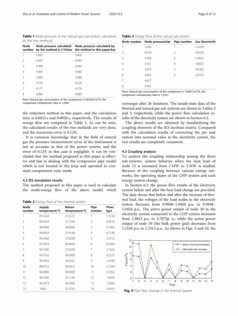
the reduction method in this paper, and the calculationtime is 0.0032 s and 0.0020 s, respectively. The results ofenergy flow are compared in Table 1. As can be seen,the calculated results of the two methods are very close,and the maximum error is 0.12%.It is common knowledge that in the field of natural

gas the pressure measurement error of the instrument isnot as accurate as that of the power system, and theerror of 0.12% in this case is negligible. It can be con-cluded that the method proposed in this paper is effect-ive and fast in dealing with the compressor pipe modelwhich is not located in the loop and operated in con-stant compression ratio mode.

4.2 IES simulation resultsThe method proposed in this paper is used to calculatethe multi-energy flow of the above model, which

converges after 26 iterations. The steady-state data of thethermal and natural gas sub-systems are shown in Tables 2and 3, respectively, while the power flow calculation re-sults of the electricity system are shown in Section 6.3.The above results are obtained by standardizing the

coupling elements of the IES Jacobian matrix. Comparedwith the calculation results of converting the per unitsystem into nominal value in the electricity system, thetwo results are completely consistent.

4.3 Coupling analysisTo analyze the coupling relationship among the threesub-systems, system behavior when the heat load ofnode 13 is increased from 1MW to 2MW is studied.Because of the coupling between various energy net-works, the operating states of the CHP system and eachenergy system change.In Section 6.3, the power flow results of the electricity

system before and after the heat load change are provided.The data shows that before and after the increase of ther-mal load, the voltages of the load nodes in the electricitysystem fluctuate from 0.9848–1.0450 p.u. to 0.9848–1.0454 p.u.. The active power output of node 30 in theelectricity system connected to the CHP system increasesfrom 2.3853 p.u. to 3.7075p .u., while the active poweroutput of node 39 (the bulk power grid) decreases from1.5520 p.u. to 1.3313 p.u.. As shown in Figs. 9 and 10, the

Table 1 Node pressure of the natural gas sub-system calculatedby the two methods

Nodenumber

Node pressure calculatedby the method in [19]/bar

Node pressure calculated bythe method in this paper/bar

1 5.000 5.000

2 4.493 4.494

3 4.480 4.480

4 4.464 4.465

5 3.485 3.488

6 4.516 4.520

7 4.171 4.176

8 4.084 4.089

Note: Natural gas consumption of the compressor is 24.0524 m3/h, thecompressor compression ratio is 1.2961

Table 2 Energy flow of the thermal system

Nodenumber

Supplytemperature/°C

Returntemperature/°C

Pipenumber

Flow/kg/s

1 99.3364 37.6222 1 7.1516

2 99.4534 37.7599 2 6.9510

3 90.4096 40.0000 3 0.2362

4 99.5624 37.9148 4 6.5146

5 99.2964 37.6206 5 3.3722

6 87.5374 40.0000 6 0.2504

7 99.1285 37.8390 7 2.7202

8 93.7532 40.0000 8 0.2215

9 99.0363 38.2022 9 2.4585

10 98.6712 38.4412 10 2.1360

11 90.4096 40.0000 11 0.2362

12 98.1056 39.1189 12 1.4939

13 96.2674 40.0000 13 1.2890

14 100.0 37.3725 14 2.9425

Table 3 Energy flow of the natural gas system

Node number Node pressure/bar Pipe number Gas flow/m3/h

1 5.000 1 7233.8

2 4.579 2 4333.8

3 4.566 3 1100.0

4 4.551 4 1800.0

5 3.874 5 4318.0

6 4.862 6 2310.0

7 4.627

8 4.581

Note: Natural gas consumption of the compressor is 19.8015 m3/h, thecompressor compression ratio is 1.2551

Fig. 9 Pipe flow change in the thermal system

Zhu et al. Protection and Control of Modern Power Systems (2021) 6:5 Page 8 of 12

related pipe flows increase in the thermal network, andthe maximum supply temperature increase of the nodes is1.8 °C. From Fig. 11, the flows in related natural gas net-work pipes also increase, while the maximum nodal pres-sure decrease is 1.0 bar. Figure 12 demonstrates thechanges of the operation of the CHP system and the bulkpower grid. Because of the CHP system working in theFTL mode, when the heat load increases, the output heatpower of the CHP is increased by 53.2% while the outputelectric power is increased by 55.5%. The natural gas con-sumption of the CHP system is also increased by 55.4%.At the same time, the electricity system takes less electri-city from the bulk power grid.

4.4 Convergence comparisonThe methods proposed in this paper and in [19] are usedto separately simulate the compressor in the IES model inFig. 8. The number of iterations of the method proposedin this paper is 26 and the simulation time is 2.440429 s.In comparison, using the method in [19], the number ofiterations is 55 and the simulation time is 3.974894 s.Thus, the method presented in this paper can be used tocalculate for a large natural gas pipeline model with com-pressors not included in the loop, as it can effectively re-duce the number of iterations and calculation time.

4.5 Discussions and extensionsThe model and multi-energy flow calculation method ofan IES proposed in this paper can be applied to actualbuildings in certain scenarios. In actual buildings, theexisting energy is electricity, gas, heat and cold, and its

steady-state model is given in this paper. The characteris-tics of cold energy and heat energy are the same so theirmodels are also the same, as both transfer energy througha heat medium. In view of the diversity of equipment con-tained in buildings, it is necessary to model flexibly ac-cording to the actual situation. If distributed generations,load fluctuation and other conditions need to be consid-ered, the dynamic or probabilistic IES multi-energy flowcalculation model should be considered.

5 ConclusionsThis paper has established the models of various energysub-systems and the coupling equipment for park levelelectricity-gas-thermal IES. On this basis, an integratedmulti-energy flow calculation model of IES is constructed.By treating the compressor separately and its pipe flowequivalent to the nodal gas load in accordance with theworking mode in a natural gas network, a simplified calcu-lation method of compressor model which is not includedin a loop and operates in constant compression ratiomode is proposed using a reduction method. In addition,a numerical conversion method for dealing with the con-flict between nominal value and per unit value in themulti-energy flow calculation of IES is described in detail.A case study is given to verify the correctness and speedof the proposed method, and the coupling interactionamong the sub-systems is also studied.General conclusions are as follows:

1. The proposed simplified calculation method for thecertain compressor category mentioned above iscorrect and fast, and this has been confirmed by thesimulation results. The system can converge within30 iterations, which constitutes a reduction of52.7%, while the calculation time is also reduced by38.6%, compared to the existing method. Thus, themethod can be particularly effective when the scaleof the system is large.

2. The technique of standardizing the coupling elementsof the IES Jacobian matrix complements some dataprocessing gaps in the calculation of integrated multi-

Fig. 10 Supply temperature change in the thermal system

Fig. 11 Pipe flow and node pressure change in the naturalgas system

Fig. 12 Operation state change of the CHP system and thebulk power grid

Zhu et al. Protection and Control of Modern Power Systems (2021) 6:5 Page 9 of 12

energy flow in an IES. This technique enables the elec-tricity system to use per unit value to participate in thecalculation and simplifies the calculation process. Re-sults are compared to the method of converting theelectricity system from per unit value to nominalvalue, and show good match, which proves the cor-rectness of the proposed technique.

3. Considering electricity-gas-thermal coupling inter-action characteristics, it can be concluded that whenthe network state of one energy sub-system in an IESchanges, the operational states of other energy sub-systems will be affected. Through the integratedmulti-energy flow calculation, the changes of nodeand equipment status in each energy sub-system canbe known in order to evaluate the rationality of thesystem, and avoid possible risks such as transformeroverload in advance. This is of great significance.

6 Appendix6.1 Mathematical expression of Jhh

Jhh ¼ Jhh11 Jhh12Jhh21 Jhh22

� ð23Þ

Jhh11 ¼∂ΔΦ∂m∂Δh f

∂m

0B@

1CA

¼ Cp diag Ts −T0ð Þf gAh1

2BhKhm

� ð24Þ

Jhh12 ¼∂ΔΦ∂Tsload

∂ΔΦ∂Trload

∂Δhf

∂Tsload

∂Δhf

∂Trload

0BB@

1CCA

¼ Cp diag Ah1mf g 00 0

� ð25Þ

Jhh21 ¼∂ΔTs

∂m∂ΔTr

∂m

0B@

1CA ¼ −

∂bs∂m∂br∂m

0B@

1CA ð26Þ

Jhh22 ¼∂ΔTs

∂Tsload

∂ΔTr

∂Trload∂ΔTs

∂Tsload

∂ΔTr

∂Trload

0BB@

1CCA ¼ Cs 0

0 Cr

� ð27Þ

6.2 Mathematical expression of Jgg

Jgg ¼ Ag1DAg1T ð28Þ

D ¼ diag12� qΔΠ

� ð29Þ

6.3 Data of the case study

Table 5 Pipeline data of the natural gas system

Pipe number Src-node Dst-node Length/m Diameter/mm

1 1 2 390 150

2 2 5 1600 150

3 2 3 500 150

4 2 4 400 150

5 6 7 600 150

6 7 8 400 150

Table 4 Gas load data of the natural gas system

Node number Gas load/m3/h

2 0

3 1100.0

4 1800.0

5 0

6 0

7 2008.0

8 Related to the CHP system

Zhu et al. Protection and Control of Modern Power Systems (2021) 6:5 Page 10 of 12

Table 8 Power flow results of the electricity system

Nodenumber

Voltage/pu Active power/pu

Before heatload increase

After heatloadincrease

Before heatload increase

After heatloadincrease

1 1.0207 1.0210 −11.9760 −11.9760

2 1.0293 1.0307 0 0

3 1.0276 1.0280 −3.2200 −3.2200

4 1.0290 1.0284 −5.0000 −5.0000

5 1.0316 1.0304 0 0

6 1.0328 1.0315 0 0

7 1.0302 1.0290 −2.3380 −2.3380

8 1.0293 1.0282 −5.2200 −5.2200

9 1.0297 1.0294 −0.0650 −0.0650

10 1.0357 1.0347 0 0

11 1.0347 1.0335 0 0

12 1.0217 1.0206 −0.0853 −0.0853

13 1.0343 1.0334 0 0

14 1.0311 1.0305 0 0

15 1.0297 1.0295 −3.2000 −3.2000

16 1.0319 1.0318 −3.2900 − 3.2900

17 1.0303 1.0304 0 0

18 1.0286 1.0288 −1.5800 −1.5800

19 1.0388 1.0388 0 0

20 0.9848 0.9848 −6.8000 −6.8000

21 1.0345 1.0344 −2.7400 −2.7400

22 1.0392 1.0392 0 0

23 1.0390 1.0390 −2.4750 −2.4750

24 1.0319 1.0319 −3.0860 −3.0860

25 1.0397 1.0404 −2.2400 −2.2400

26 1.0349 1.0353 −1.3900 −1.3900

27 1.0307 1.0309 −2.8100 −2.8100

28 1.0404 1.0408 −2.0600 −2.0600

29 1.0450 1.0454 −2.8350 −2.8350

30 1.0499 1.0499 2.3853 3.7075

31 1.0300 1.0300 10.0000 10.0000

32 0.9841 0.9841 6.5000 6.5000

33 0.9972 0.9972 6.3200 6.3200

34 1.0123 1.0123 5.0800 5.0800

35 1.0494 1.0494 6.5000 6.5000

36 1.0636 1.0636 5.6000 5.6000

37 1.0275 1.0275 5.4000 5.4000

38 1.0265 1.0265 8.3000 8.3000

39 0.9820 0.9820 8.1845 6.8524

Table 7 Pipeline Data of the thermal system

Pipe number Src-node Dst-node Length/m Diameter/mm

1 14 1 1000 150

2 1 2 800 150

3 2 3 500 150

4 2 4 600 150

5 4 5 500 150

6 5 6 700 150

7 5 7 500 150

8 7 8 300 150

9 7 9 500 150

10 9 10 600 150

11 10 11 500 150

12 10 12 600 150

13 12 13 700 150

14 13 13 2500 150

Table 6 Heat load data of the thermal system

Node number Heat power/W Output temperature/°C

1 50,000 40

2 50,000 40

3 50,000 40

4 50,000 40

5 100,000 40

6 50,000 40

7 10,000 40

8 50,000 40

9 80,000 40

10 100,000 40

11 50,000 40

12 50,000 40

13 100,000 40

Zhu et al. Protection and Control of Modern Power Systems (2021) 6:5 Page 11 of 12

AbbreviationsIES: Integrated energy system; GA: Genetic algorithm; GEF: Generalizedenergy flow; CHP: Combined heat and power; FTL: Following the thermalload

AcknowledgmentsNot applicable.

Authors’ contributionsM. Zhu, the main author of this study, her contributions included the idea,mathematical and practical design, case study and writing the paper. S.Dong, the corresponding author, he guided the study at all stage andimproved the text. C. Xu, K. Tang and C. Gu, the supervisors of the study,their reviewed and improved the text. The author(s) read and approved thefinal manuscript.

FundingThis work was supported by National Natural Science Foundation of China(52077193).

Availability of data and materialsAll data generated or analyzed during this study are included in thepublished article (and its supplementary information files).

Competing interestsThe authors declare that they have no competing interests.

Author details1College of Electrical and Engineering, Zhejiang University, Zhejiang, China.2The Department of Electronic and Electrical Engineering, University of Bath,Bath BA2 7AY, UK.

Received: 9 July 2020 Accepted: 18 January 2021

References1. Li, J., Huang, Y., & Zhang, P. (2018). Review of multi-energy flow calculation

model and method in integrated energy system. Electric Power Construction,39(3), 1–11. https://doi.org/10.3969/j.issn.1000-7229.2018.03.001.

2. Meng, B., Guo, F., Hu, L., Bai, X., & Liu, C. (2019). Wind abandonment analysisof multi-energy systems considering gas-electrical coupling. Electric PowerEngineering Technology, 38(6), 2–8. https://doi.org/10.12158/j.2096-3203.2019.06.001.

3. Dai, X., Han, X., Dong, Y., Luo, H., & Li, Y. (2019). Multi-source and multi-levelcoordination optimization method of energy internet. Electric PowerEngineering Technology, 38(2), 1–9. https://doi.org/10.19464/j.cnki.cn32-1541/tm.2019.02.001.

4. Chen, L., Wu, J., Tang, H., Xiong, Y., & Li, C. (2019). Optimal allocation modelof the micro-energy grid with CCHP considering renewable energyconsumption. Electric Power Engineering Technology, 38(5), 121–129. https://doi.org/10.12158/j.2096-3203.2019.05.018.

5. Zhong, J., Li, Y., Zeng, Z., & Cao, Y. (2019). Quasi-steady-state analysis andcalculation of multi-energy flow for integrated energy system. Electric PowerAutomation Equipment, 39(08), 22–30. https://doi.org/10.16081/j.epae.201908010.

6. Chen, B., Sun, H., Wu, W., Guo, Q., & Qiao, Z. (2020). Energy circuit theory ofintegrated energy system analysis (III): Steady and dynamic energy flowcalculation. Proceedings of the Chinese Society of Electrical Engineering, 40(15),4820–4831. https://doi.org/10.13334/j.0258-8013.pcsee.200647.

7. Gomezexposito, A., Canizares, C., & Conejo, A. J. (2008). Electric energysystems. Crc Press.

8. Gandomkar, M., Mirsaeidi, S., & Miveh, M. (2012). Distribution system modelingand analysis. Tehran: Gheddis Press.

9. Tang, K., Dong, S., & Song, Y. (2020). Successive-intersection-approximation-based power flow method for integrated transmission and distributionnetworks. IEEE Transactions on Power Apparatus and Systems, 35(6), 4836–4846. https://doi.org/10.1109/TPWRS.2020.2994312.

10. Tang, K., Dong, S., Shen, J., & Song, Y. (2019). A robust and efficient two-stage algorithm for power flow calculation of large-scale systems. IEEETransactions on Power Systems, 34(6), 5012–5022. https://doi.org/10.1109/TPWRS.2019.2914431.

11. Jiang, M., Wang, S., & Zeng, Z. (1995). Simulation and analysis of gastransmission and distribution network. Beijing: Petroleum Industry Press.

12. Yu, D. (2019). Modeling and analysis optimal energy flow in combined heatingand electrical multi-energy system considering the linear network constraints.North China Electric Power University (in Beijing). https://kns.cnki.net/KCMS/detail/detail.aspx?dbname=CMFD202001&filename=1019240086.nh.

13. Yuan, Z., Zhao, Y., Guo, Z., et al. (2019). Research summary of integrated energysystems planning for energy internet. Southern Power System Technology, 13(7),1–9. https://doi.org/10.13648/j.cnki.issn1674-0629.2019.07.001.

14. Guo, Z., Lei, J., Ma, X., Yuan, Z., Dong, B., & Yu, H. (2019). Modeling andcalculation methods for multi-energy flows in large-scale integrated energysystem containing electricity, gas, and heat. Proceedings of the CSU-EPSA,31(10), 96–102. https://doi.org/10.19635/j.cnki.csu-epsa.000283.

15. Li, Q., An, S., & Gedra, T. W. (2003). Solving natural gas load flow problemsusing electric load flow techniques. In Proceedings of the North AmericanPower Symposium.

16. Xie, H., & Hu, L. (2017). Power flow calculation of combined heat andelectricity system. Distribution & Utilization, 34(12), 21–26. https://doi.org/10.19421/j.cnki.1006-6357.2017.12.004.

17. Liu, X. (2013). Combined analysis of electricity and heat networks. Cardiff:Cardiff University.

18. Liu, X., Wu, J., Jekins, N., & Bagdanavicius, A. (2016). Combined analysis ofelectricity and heat networks. Applied Energy, 162, 1238–1250. https://doi.org/10.1016/j.apenergy.2015.01.102.

19. Wang, Y., Zeng, B., Guo, Z., & Zhang, J. (2016). Multi-energy flow calculationmethod for integrated energy system containing electricity, heat and gas.Power System Technology, 40(10), 2942–2950. https://doi.org/10.13335/j.1000-3673.pst.2016.10.004.

20. Zhao, X., Yang, L., Qu, X., & Yan, W. (2018). An improved energy flowcalculation method for integrated electricity and natural gas system.Transactions of China Electrotechnical Society, 33(3), 467–477. https://doi.org/10.19595/j.cnki.1000-6753.tces.161923.

21. Yu, X., & Zhao, J. (2018). Heat-gas-power flow calculation method forintegrated energy system containing P2H and P2G. Electric PowerConstruction, 39(12), 13–21.

22. Shi, J., Wang, L., Wang, Y., & Zhang, J. (2017). Generalized energy flowanalysis considering electricity gas and heat subsystems in local-area energysystems integration. Energies, 10(4), 514. https://doi.org/10.3390/en10040514.

23. Magdy, G., Mohamed, E., Shabib, G., Elbaset, A., & Mitani, Y. (2018). Microgriddynamic security considering high penetration of renewable energy.Protection and Control of Modern Power Systems, 3(3), 236–246. https://doi.org/10.1186/s41601-018-0093-1.

24. Mohammed, A., Li, L., Jiang, L., & Tang, W. (2018). Residue theorem basedsoft sliding mode control for wind power generation systems. Protectionand Control of Modern Power Systems, 3(3), 247–258. https://doi.org/10.1186/s41601-018-0097-x.

25. Wood, J. (2008). Combined heat and power. Local Energy: Distributedgeneration of heat and power. IET Digital Library.

26. Yan, J., Huang, J., & He, M. (2006). The technology of CCHP. Beijing: ChemicalIndustry Press.

27. Public Utility Regulatory Policies Act of 1978 (1982). Annual report tocongress. United States.

Zhu et al. Protection and Control of Modern Power Systems (2021) 6:5 Page 12 of 12