This is a repository copy of An integrated, multi-scale modelling approach for the simulation of multiphase dispersion from accidental CO2 pipeline releases in realistic terrain.

White Rose Research Online URL for this paper:http://eprints.whiterose.ac.uk/81674/

Article:

Woolley, RM, Fairweather, M, Wareing, CJ et al. (15 more authors) (2014) An integrated, multi-scale modelling approach for the simulation of multiphase dispersion from accidental CO2 pipeline releases in realistic terrain. International Journal of Greenhouse Gas Control,27. 221 - 238. ISSN 1750-5836

https://doi.org/10.1016/j.ijggc.2014.06.001

eprints@whiterose.ac.ukhttps://eprints.whiterose.ac.uk/

Reuse

Unless indicated otherwise, fulltext items are protected by copyright with all rights reserved. The copyright exception in section 29 of the Copyright, Designs and Patents Act 1988 allows the making of a single copy solely for the purpose of non-commercial research or private study within the limits of fair dealing. The publisher or other rights-holder may allow further reproduction and re-use of this version - refer to the White Rose Research Online record for this item. Where records identify the publisher as the copyright holder, users can verify any specific terms of use on the publisher’s website.

Takedown

If you consider content in White Rose Research Online to be in breach of UK law, please notify us by emailing eprints@whiterose.ac.uk including the URL of the record and the reason for the withdrawal request.

An Integrated, Multi-scale Modelling Approach for the Simulation of Multiphase Dispersion from Accidental CO2

Pipeline Releases in Realistic Terrain

R.M. Woolleya, M. Fairweatherb, and C.J. Wareingc,

abc

School of Process, Environmental and Materials Engineering,

Institute of Particle Science and Engineering,

University of Leeds, Leeds LS2 9JT, UK. a

Tel: +44 (0) 113 343 2351

r.m.woolley@leeds.ac.uk (corresponding author)

Fax: +44 (0) 113 343 2384 bm.fairweather@leeds.ac.uk

c

c.j.wareing@leeds.ac.uk

C. Prouste, J. Hebrardf

D. Jamois, and

g

efg

Parc Technologique ALATA, INERIS, Dept. PHDS,

BP 2, 60550 Verneuil-en-Halatte, France. echristophe.proust@ineris.fr

fjerome.hebrard@ineris.fr g

didier.jamois@ineris.fr

V.D. Narasimhamurthyl, I.E. Storvikm

and T. Skjold,

n

l

P.O. Box 6015, Bergen Bedriftssenter, GexCon AS,

NO-5892 Bergen, Norway. lvagesh@gexcon.com

midar@gexcon.com n

trygve@gexcon.com

S.A.E.G. Falled

d

University of Leeds, Leeds LS2 9JT, UK. School of Mathematics,

d

s.a.e.g.falle@leeds.ac.uk

S. Brownh, H. Mahgereftehi

and S. Martynov,

j hij

University College London, Department of Chemical Engineering,

London WC1E 7JE, UK. hsolomon.brown@ucl.ac.uk ih.mahgerefteh@ucl.ac.uk

j

s.martynov@ucl.ac.uk

S.E. Gantk

k

Harpur Hill, Health & Safety Laboratory,

Buxton SK17 9JN, UK. k

Simon.Gant@hsl.gsi.gov.uk

D.M. Tsangariso, I.G. Economoup*

G.C. Boulougouris,

q, and N.I. Diamantonisr

opqr

GR–153 10 Aghia Paraskevi Attikis, Greece.

National Center for Scientific Research “Demokritos”, Institute of Physical

Chemistry, Molecular Thermodynamics and Modelling of Materials Laboratory,

odtsangaris@chem.demokritos.gr p

economou@chem.demokritos.gr

qgboul@chem.demokritos.gr r

*Current address: Chemical Engineering Program, Texas A&M University at Qatar,

PO Box 23874, Doha, Qatar

nidiama@chem.demokritos.gr

Submission of a full-length article to the International Journal of Greenhouse Gas Control, of

unpublished material not submitted for publication elsewhere

Running title: Integrated Modelling of Accidental CO2

© CROWN COPYRIGHT 2014 Releases

ABSTRACT

The deployment of a complete carbon capture and storage chain requires a focus upon the

hazards posed by the operation of pipelines transporting carbon dioxide (CO2) at high

pressure in a dense-phase (supercritical or liquid state). The consequences of an intentional or

accidental release from such pipelines must be considered as an integral part of the design

process. There are a number of unique challenges to modelling these releases due to the

unusual phase-transition behaviour of CO2. Additionally, few experimental observations of

large-scale CO2 releases have been made, and the physics and thermochemistry involved are

not fully understood. This work provides an overview of elements of the EC FP7

CO2PipeHaz project, whose overall aim is to address these important and pressing issues,

and to develop and validate mathematical models for multiphase discharge and dispersion

from CO2 pipelines. These are demonstrated here upon a full-scale pipeline release scenario,

in which dense-phase CO2 is released from a full-bore 36-inch pipeline rupture into a crater,

and the resulting multiphase CO2

plume disperses over complex terrain, featuring hills and

valleys. This demonstration case is specifically designed to illustrate the integration of

different models for the pipeline outflow, near-field and far-field dispersion.

KEYWORDS

CCS, CO2

, multi-phase flow, experimental measurement, mathematical modelling, pipeline

depressurisation

1. INTRODUCTION

Carbon capture and storage (CCS) is a set of technologies designed to reduce CO2 emissions

from large point-sources of production such as coal-fired power stations and other industrial

facilities. It involves the capture of CO2 and its storage in suitable semi-permanent reservoirs

such as naturally formed saline aquifers or depleted oil wells, instead of allowing its release

to the atmosphere where it contributes to climate change. In most of the planned CCS

projects, the CO2 is transported from the capture to the storage sites in high-pressure

pipelines, typically operating at pressures above 80 bar, where the CO2

Whilst the physics of high-pressure releases of substances such as natural gas and propane is

relatively well understood (

is in either a

supercritical or liquid state, depending upon whether it is above or below the critical

temperature of 304.19 K.

Cowley and Tam, 1988; Richardson and Saville, 1996), CO2

possesses some unusual physical properties which make its release behaviour more

challenging to predict. As pure CO2, its triple-point pressure and temperature are 5.18 bar

and 216.55 K respectively, and at atmospheric pressure CO2 exists in either a solid or

gaseous state, with a sublimation temperature of 194.25 K. This means that there is likely to

be complex phase-transition when CO2

2009

decompresses from an initial dense-phase state in the

pipeline (i.e. as a supercritical or liquid fluid) into a solid and gaseous state at atmospheric

pressure. The work undertaken in the EC FP7 CO2PipeHaz project ( ) has been pivotal to

improving the understanding of this complex phase-transition behaviour and providing more

accurate predictions of the consequence associated with CO2

CO

pipeline releases.

2

NIOSH,

1996

is a colourless and odourless gas under ambient conditions, and is toxic if inhaled in air

at concentrations around 5%, and likely to be fatal at concentrations of around 10% (

). Liquid CO2 has a density approximately 50% less than that of water, but has a

viscosity of magnitude more frequently associated with gases, and this property makes the

transport of CO2 an economically viable and attractive proposition. However, preliminary

calculations and experimental evidence indicate that, due to it possessing a relatively high

Joule-Thomson expansion coefficient, the rapid expansion of an accidental liquid release may

reach temperatures below 180 K. Due to this effect, solid formation following a pipeline

puncture or rupture is to be expected, and subsequently, at atmospheric pressure, the solid

CO2 will sublime into gas. In assessing the hazards posed by releases of CO2, it is important

to take account of the fact that the CO2 gas will be much denser than air, due to both its

higher molecular weight and very low temperature. This could lead to a gravity-driven flow

of high CO2

The modelling of outflow and subsequent atmospheric dispersion following pipeline failure is

especially challenging given the large number of complex and often interacting processes

governing the phenomena involved. The rupture of the pipeline results in a series of

expansion waves that propagate into the undisturbed fluid in the pipe towards the intact end

of the pipeline. These waves result in the acceleration of the fluid particles in the opposite

direction and hence outflow. The precise tracking of these expansion waves and their

propagation as a function of time and distance along the pipeline is necessary for the accurate

prediction of the outflow, as well as any propagating fractures within the pipeline material.

This involves detailed consideration of several processes including heat and mass transfer,

unsteady fluid flow and thermodynamics (

-concentration gas, which would tend to flow down slopes and accumulate in

low-lying areas.

Mahgerefteh et al., 2012a). Additionally, given that

the transportation of CO2 will undoubtedly occur at high pressure, this means that the near-

isentropic expansion resulting from a pipeline failure will likely induce two-phase flow. The

modelling of the subsequent dispersion of CO2

This paper describes the development of novel multi-phase pipeline discharge and dispersion

models applicable to dense-phase CO

in the atmosphere also poses a number of

difficulties due to the complex interaction of a number of physical and thermodynamic

phenomena including the formation of stationary shock-cell structures, phase transition, and

the behaviour of multi-phase systems. In the case of a full-bore rupture, this will inevitably

occur within the confines of a crater excavated by the high-pressure release and the geometry

of this crater will invariably affect the near-field dispersion of the release. Hence, this must

be considered if suitable source terms are to be provided to the far-field dispersion models.

Finally, the far-field atmospheric dispersion phenomena can only truly be understood if the

fluid dynamics of the release are evaluated using a realistic terrain in which the effects of

gravitational acceleration, buoyancy, wind, turbulence, and the behaviour of the different

phases are considered.

2 pipelines, and their validation against recently

obtained experimental data. The accidental release considered was of pure CO2

2013

, initially at

150 bar and 283 K, from a pipeline 217 km in length and with an internal diameter of 0.914

m (36 inches). A full-bore guillotine rupture was modelled, which was assumed to take place

84 km from the feed-end of the pipeline. Terrain data obtained from the UK Ordnance Survey

database ( ) was incorporated into the modelling to represent a realistic release scenario.

2. VALIDATORY EXPERIMENTAL WORK

Although it is clearly not possible to validate the overall model which integrates pipe-flow,

pipe-release, near-field and far-field dispersion modelling, the accuracy of certain elements of

the models was assessed against large-scale data acquired as part of the project.

Figure 1 shows a schematic of the rig and the sensor arrays used at INERIS for the

experimental studies of large-scale CO2

Jamois et al., 2013

releases. The rig was used to acquire data regarding

mass flow-rates, and near-field temperature and concentration distributions in a number of

different release scenarios of varying nozzle sizes and initial pressures. These data have been

used in the validation of the in-pipe, near-field, and far-field dispersion models, and further

details can be found in the literature ( ). Part of this validation is discussed

below, but further information be found in recent CO2PipeHaz project reports (Fairweather et

al., 2011; Martynov, 2013; Narasimhamurthy et al., 2013).

In the flow field, the instrumentation consisted of twenty-six, radially distributed

thermocouples, and six oxygen depletion sensors distributed along the centre-line axis of the

jet. The region used for the near-field dispersion-model validation extended to 5 m from the

release plane. This choice of the modelling domain size was due to the near-field model

developments in this paper being concerned with the accurate representation of under-

expanded, shock-laden, multi-phase jets, and the structure of their initial expansion to

atmospheric conditions. By 5 m downstream of the release point, the jet has become self-

similar in its properties, and has been at atmospheric pressure for a considerable distance.

Hence, the modelling of the far-field region does not require such specialist treatment.

Figure 2 is a schematic of the release vessel, supported by photographs of the assembly

including the release valve, stop valves, and the discharge orifice. The 2 m3 spherical

pressure vessel was thermally insulated, and can contain up to 1000 kg of CO2 at a maximum

operating pressure and temperature of 200 bar and 473 K, respectively. It is equipped

internally with 6 thermocouples and 2 high-precision pressure gauges, and was connected to a

discharge line of 50 mm inner diameter, with no internal restrictions. In total, the line is 9 m

long including a bend inside the vessel, plunging to the bottom in order to ensure that it was

fully submersed in liquid CO2. Three ball valves were installed in the pipe. Two were

positioned close to the vessel and the third near to the orifice holder. The first valve closest to

the sphere was a manual safety valve, and the two others were remotely actuated. All valves

were full-bore ball valves, sized appropriately for the pipe section.

The vessel was supported by four Mettler 0745 A load cells, enabling a continuous

measurement of the CO2

Various orifices were used at the exit plane of the discharge pipe, which were drilled into a

large screwed flange. Figure 4 is a schematic of such, where the thickness of this flange (E) is

9 mm for the 6mm orifice and 15 mm for the 25 mm orifice. The diameter of the orifice (f)

is constant over a length of 5 mm or 10 mm (e) and then expands with an angle of 45°

towards the exterior.

content with an uncertainty of plus or minus 0.5 kg. The

determination of the mass flow-rate was performed within an accuracy of approximately

10%, mainly due to the noise present in the measurement signal during the release. These

obtained measurements have been used to assist in the validation of the pipe out-flow models.

In the sphere, the pressure was measured using a Piezoresistive type KISTLER 4045 A 200

sensor with a range of 0 to 200 bar and an accuracy of plus or minus 0.1%. This sensor was

mounted directly to the flange of the sphere, as shown in Figure 3. Another Piezoresistive

type KISTLER 4045 A 500 sensor, with a range of 0 to 500 bar, was connected to the sphere

and served as a backup. The internal temperature of the vessel was measured at 6 points on

the vertical axis of the sphere using 1mm sheathed, type K thermocouples, with an accuracy

of plus or minus 0.25 K. Temperature immediately upstream of the orifice was similarly

measured. The static pressure immediately upstream from the orifice was measured using a

KULITE 0-350 bar instrument with an accuracy of ±0.5%. The vessel instrumentation is

shown in Figure 3.

3. IN-PIPE AND RELEASE-CONDITION M ODELLING

3.1 Modelling Approach

To date, the majority of the pipeline outflow models reported in the literature have utilised

the homogeneous equilibrium model (HEM) (Mahgerefteh et al., 1999; Mahgerefteh and

Wong, 1999; Popescu, 2009; Webber et al., 1999) where the constituent fluid phases are

assumed to remain in thermal and mechanical equilibrium during the decompression process.

In contrast to the HEM, the homogeneous relaxation model (HRM) accounts for the delay in

vaporisation during the decompression process using an empirical relaxation equation for the

mass fraction of vapour phase, while assuming that the constituent phases are in mechanical

equilibrium, i.e. that they move at the same velocity. In the HRM, the mass, momentum,

energy and vapour quality conservation equations are respectively given by (Brown et al.,

2013):

( ) 0ut x

ρ ρ∂ ∂+ =

∂ ∂ (1)

( ) ( )2

2 wf uu u p

t x d

ρρ ρ∂ ∂+ + = −

∂ ∂ (2)

( ) ( )( )2

wf uE u E p u

t x d

ρρ∂ ∂+ + =−

∂ ∂ (3)

( ) ( ) equt x

α αρα ρ α ρ

τ−∂ ∂

+ =∂ ∂

(4)

where ρ , u , p , d , wf , α , and τ are respectively the mixture density, velocity, pressure,

pipeline diameter, Fanning friction factor calculated using Chen’s correlation (Chen, 1979),

the dynamic vapour quality and a relaxation time accounting for the delay in the phase

change transition as functions of time, t , and space, x . E represents the total mixture energy

defined as:

21

2E e uρ = +

(5)

where e is specific internal energy of the mixture:

( ) ( )1sv mle e p eα α= + − (6)

and ρ is the mixture density given by:

( )( )( )

11

,sv ml mlp p e

ααρ ρ ρ

−= + (7)

In equations (6) and (7), the subscripts sv and ml respectively refer to the saturated vapour

and meta-stable liquid phases, which may be at different temperatures.

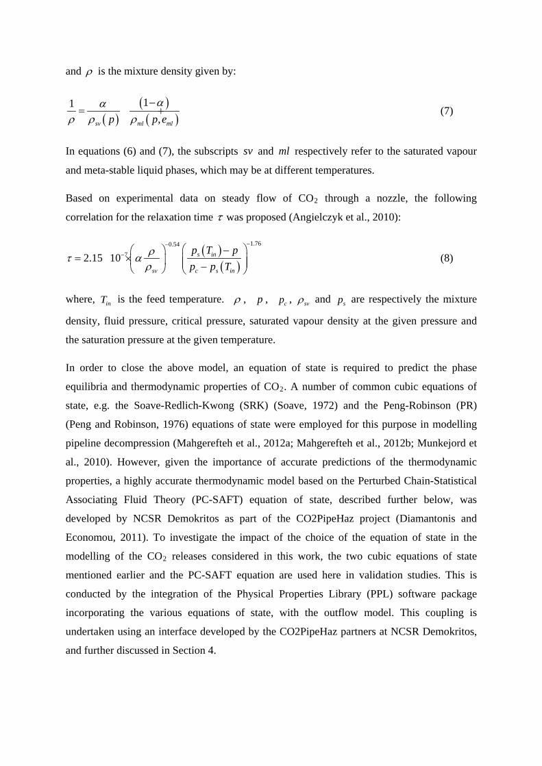
Based on experimental data on steady flow of CO2

τ

through a nozzle, the following

correlation for the relaxation time was proposed (Angielczyk et al., 2010):

( )( )

1.760.54

72.15 10 s in

sv c s in

p T p

p p T

ρτ αρ

−−

− − = × −

(8)

where, inT is the feed temperature. ρ , p , cp , svρ and sp are respectively the mixture

density, fluid pressure, critical pressure, saturated vapour density at the given pressure and

the saturation pressure at the given temperature.

In order to close the above model, an equation of state is required to predict the phase

equilibria and thermodynamic properties of CO2

Soave, 1972

. A number of common cubic equations of

state, e.g. the Soave-Redlich-Kwong (SRK) ( ) and the Peng-Robinson (PR)

(Peng and Robinson, 1976) equations of state were employed for this purpose in modelling

pipeline decompression (Mahgerefteh et al., 2012a; Mahgerefteh et al., 2012b; Munkejord et

al., 2010). However, given the importance of accurate predictions of the thermodynamic

properties, a highly accurate thermodynamic model based on the Perturbed Chain-Statistical

Associating Fluid Theory (PC-SAFT) equation of state, described further below, was

developed by NCSR Demokritos as part of the CO2PipeHaz project (Diamantonis and

Economou, 2011). To investigate the impact of the choice of the equation of state in the

modelling of the CO2 releases considered in this work, the two cubic equations of state

mentioned earlier and the PC-SAFT equation are used here in validation studies. This is

conducted by the integration of the Physical Properties Library (PPL) software package

incorporating the various equations of state, with the outflow model. This coupling is

undertaken using an interface developed by the CO2PipeHaz partners at NCSR Demokritos,

and further discussed in Section 4.

The HRM has recently been applied to the modelling of CO2

Brown et al., 2013

discharge following full-bore

rupture of pipelines ( ) where it was shown to produce reasonable

agreement in comparison with available experimental data. As a further validation, this model

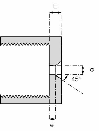
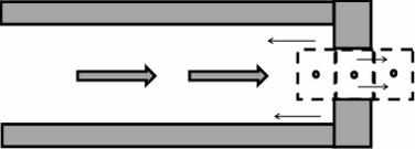
has been applied to predict outflow from pipelines with small diameter punctures. For

modelling purposes, a pipeline with an orifice at the release end is considered as depicted in

Figure 5.

Given that the model described by equations (1) to (4) can only be solved numerically, an

operator splitting method is used (LeVeque, 2002). This method breaks the solution down

into two steps: firstly the conservative left-hand-side of equations (1) to (4) are solved using

an upwind, flux differencing scheme based on the Harten, Lax, van Leer (HLL) approximate

Riemann solver (Harten et al., 1983). Secondly, this solution is updated by solving a system

of ordinary differential equations incorporating the expressions on the right-hand-side of

equations (1) to (4). Full details of the algorithm are described in Brown et al. (2013).

3.2 Validation, Results and Discussion

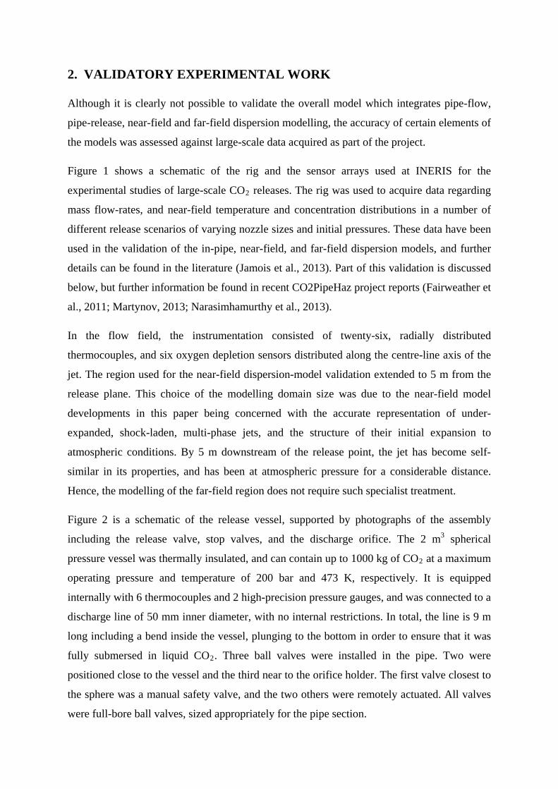
The model described above has been applied to the simulation of flow through the

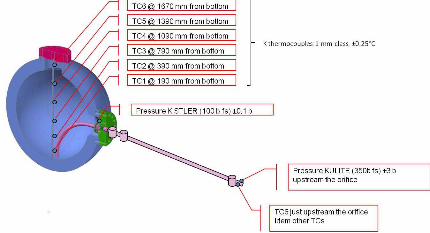
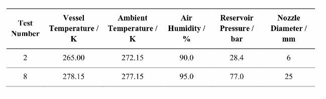
experimental apparatus described in Section 2. Table 1 summarises the conditions of two

tests chosen for the model validation in the present work. As can be seen from this table, the

tests were performed using release orifices of two different diameters and two different initial

vessel pressures and temperatures. Given that the focus of this study was to replicate the

steady release through a puncture in a pipeline, the vessel initial pressures were assumed to

be constant and simulations were run until a steady release rate was obtained.

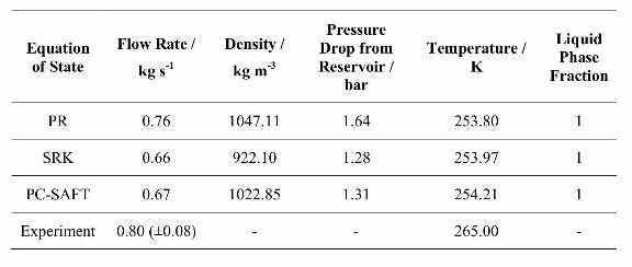
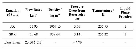
Table 2 shows the mass flow rate, pressure drop from the reservoir, temperature and density

of the CO2 fluid at the release orifice, as predicted by the outflow model using the PR, SRK

and PC-SAFT equations of state respectively for Test 2, as well as the measured mass flow

rate. It can be seen that the results obtained using the PR equation are the most conforming

with experimental observation with respect to prediction of the mass flow rate, while both the

SRK and PC-SAFT equations slightly under-predict the experimental values. Similarly, a

lower release pressure is obtained with the PR as compared to the SRK and PC-SAFT

equations, while the SRK predicts a markedly lower density. Interestingly, all predictions

indicate that the CO2

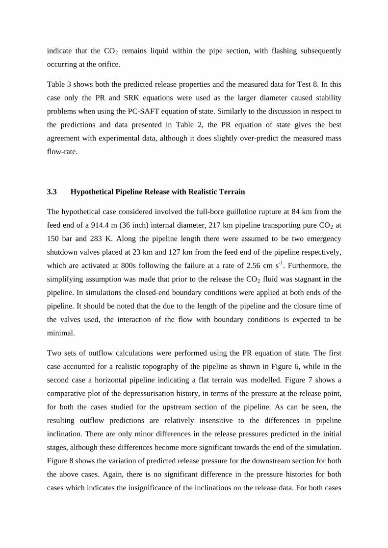
Table 3 shows both the predicted release properties and the measured data for Test 8. In this

case only the PR and SRK equations were used as the larger diameter caused stability

problems when using the PC-SAFT equation of state. Similarly to the discussion in respect to

the predictions and data presented in Table 2, the PR equation of state gives the best

agreement with experimental data, although it does slightly over-predict the measured mass

flow-rate.

remains liquid within the pipe section, with flashing subsequently

occurring at the orifice.

3.3 Hypothetical Pipeline Release with Realistic Terrain

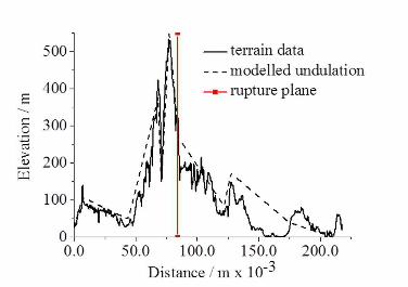
The hypothetical case considered involved the full-bore guillotine rupture at 84 km from the

feed end of a 914.4 m (36 inch) internal diameter, 217 km pipeline transporting pure CO2 at

150 bar and 283 K. Along the pipeline length there were assumed to be two emergency

shutdown valves placed at 23 km and 127 km from the feed end of the pipeline respectively,

which are activated at 800s following the failure at a rate of 2.56 cm s-1. Furthermore, the

simplifying assumption was made that prior to the release the CO2

Two sets of outflow calculations were performed using the PR equation of state. The first

case accounted for a realistic topography of the pipeline as shown in Figure 6, while in the

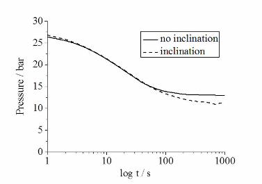
second case a horizontal pipeline indicating a flat terrain was modelled. Figure 7 shows a

comparative plot of the depressurisation history, in terms of the pressure at the release point,

for both the cases studied for the upstream section of the pipeline. As can be seen, the

resulting outflow predictions are relatively insensitive to the differences in pipeline

inclination. There are only minor differences in the release pressures predicted in the initial

stages, although these differences become more significant towards the end of the simulation.

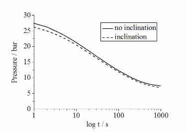
Figure 8 shows the variation of predicted release pressure for the downstream section for both

the above cases. Again, there is no significant difference in the pressure histories for both

cases which indicates the insignificance of the inclinations on the release data. For both cases

fluid was stagnant in the

pipeline. In simulations the closed-end boundary conditions were applied at both ends of the

pipeline. It should be noted that the due to the length of the pipeline and the closure time of

the valves used, the interaction of the flow with boundary conditions is expected to be

minimal.

the predicted release pressure is approximately 7 bar by the end of the simulation. Finally,

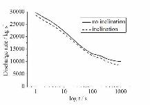
Figure 9 shows the total predicted discharge rate variation, from both ends of the pipeline,

plotted against time for both cases. The flow rate predicted for the two cases is coincidental

over much of the simulation duration. This result indicates that for the given terrain, the

variation of the pipeline inclination has a small effect on the release. This lack of impact is

explained by the relatively small contribution of the hydrostatic head to the total pressure in

the pipeline during the initial period of its depressurisation.

4. THERMODYNAMIC PROPER TY MODELLING

Accurate and efficient prediction of thermodynamic properties of pure CO2 and its mixtures

with non-condensable gases of interest to CCS is key to successful modelling of accidental

CO2

Tsangaris et al., 2013

releases from pressurised transportation pipelines. The Physical Properties Library

(PPL) ( ) developed by NCSR Demokritos encapsulates a variety of

thermodynamic methods capable of predicting these properties as functions of temperature,

pressure and composition. Existing models applicable to CO2

2013

transportation conditions have

been recently reviewed by Diamantonis et al. ( ). The PPL can predict properties such as

density, fugacity, enthalpy, and viscosity using empirical, semi-empirical and theoretical

models available in the literature or recently developed for CO2

Thermodynamic models for pure components and mixtures are often based on pure

component constants such as molecular weight, critical properties, or an acentric factor. The

PPL has an internal database that stores these pure component values and model parameters,

and hence physical properties of pure components such as liquid density, heat capacity, speed

of sound, and Joule-Thompson coefficient can be calculated by a number of different models

available in the literature. The PPL supports the most popular models available including

equations of state and empirical equations. It also supports the prediction of CO

within the scope of this

work.

2

For CO

mixture

properties using popular models. These include cubic equations of state such as Redlich-

Kwong (RK), Soave-Redlich-Kwong, and Peng-Robinson, specialized equations of state such

as GERG, and advanced equations of state such as SAFT, PC-SAFT, and tPC-PSAFT.

2 and CO2

• Volumetric (density, compressibility)

mixtures, the PPL can be used to obtain the following properties:

• Energy related (enthalpy, entropy, heat capacity)

• Free energy (Gibbs, fugacity)

• Derivative (Joule-Thomson, speed of sound)

• Transport (viscosity, diffusivity, thermal conductivity)

and the equilibrium properties can be obtained using the following methods:

• Cubic equations of state (RK, SRK, PR)

• Specialized equations of state (GERG)

• Advanced equations of state (SAFT/PC-SAFT/tPC-PSAFT)

• Empirical and semi-empirical models

The end user can select the desired method of calculation and the physical property of interest

through appropriate library ‘calls’ and ‘options’ as described in the published Advanced

Programming Interface (Tsangaris et al., 2013).

4.1 SAFT and PC-SAFT Equations of State

The focus of this work has been the development of accurate thermodynamic models for pure

CO2

( )R hs disp chain assocA A A A A= + + +

and its mixtures with non-condensable gases for the temperature range of interest, based

upon the SAFT family of equations of state. These equations of state combine an increase in

accuracy compared to the cubic methods, and a reduced computational overhead compared to

specialized formulations such as GERG. A brief description of SAFT follows. It is written as

a summation of residual Helmholtz free energy terms that occur due to different types of

molecular interactions in the system under consideration. This can be expressed as:

(9)

where:

( )22

1

34

n

nn

RT

Ahs

−−

= is the hard-sphere term (Carnaham-Starling) (10)

∑∑= =

=

4

1

9

1i j

ji

ij

disp n

kT

uD

RT

A

τ is the dispersion term (Adler equation) (11)

( )( )31

5.01ln1

n

nm

RT

Achain

−−

−= is the chain term (Wertheim) (12)

and ∑=

+

−=

M

A

AA

assoc

MX

XRT

A

1 21

2ln is the association term (Wertheim) (13)

with

3

3exp1

−−==

kT

uCmvmvn

oooo τρτρ (14)

+=

kT

e

k

u

k

u o

1 (15)

∑=

ΑΒ∆+=

M

B

B

A

X

X

1

1

1

ρ (16)

( ) ( )ABAB

seg

kTdg κσε 31exp

−

=∆ΑΒ (17)

( ) ( )( )31

21

n

n

dgdg hsseg

−

−=≈ (18)

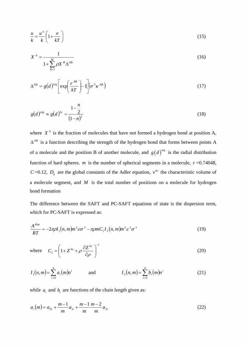
where AX is the fraction of molecules that have not formed a hydrogen bond at position A,

ΑΒ∆ is a function describing the strength of the hydrogen bond that forms between points A

of a molecule and the position B of another molecule, and ( )segg d is the radial distribution

function of hard spheres. m is the number of spherical segments in a molecule, τ =0.74048,

C =0.12, ijD are the global constants of the Adler equation, oov the characteristic volume of

a molecule segment, and M is the total number of positions on a molecule for hydrogen

bond formation

The difference between the SAFT and PC-SAFT equations of state is the dispersion term,

which for PC-SAFT is expressed as:

( ) ( ) 32221

321 ,,2 σεπρεσπρ mmnImCmmnI

RT

Adisp

−−= (19)

where 1

1 1−

∂∂

++=ρ

ρhc

hs ZZC (20)

( ) ( )∑=

=6

01 ,

i

ii nmamnI and ( ) ( )∑

=

=6

02 ,

i

ii nmbmnI (21)

while ia and ib are functions of the chain length given as:

( ) iiii am

m

m

ma

m

mama 210

211 −−+

−+= (22)

( ) iiii bm

m

m

mb

m

mbmb 210

211 −−+

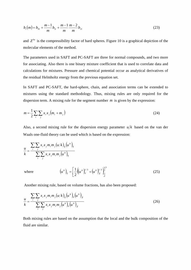
−+= (23)

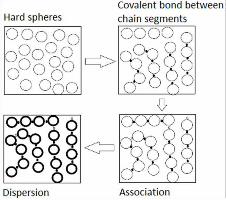
and hsZ is the compressibility factor of hard spheres. Figure 10 is a graphical depiction of the

molecular elements of the method.

The parameters used in SAFT and PC-SAFT are three for normal compounds, and two more

for associating. Also there is one binary mixture coefficient that is used to correlate data and

calculations for mixtures. Pressure and chemical potential occur as analytical derivatives of

the residual Helmholtz energy from the previous equation set.

In SAFT and PC-SAFT, the hard-sphere, chain, and association terms can be extended to

mixtures using the standard methodology. Thus, mixing rules are only required for the

dispersion term. A mixing rule for the segment number m is given by the expression:

( )∑∑ +=i j

jiji mmxxm2

1 (24)

Also, a second mixing rule for the dispersion energy parameter ku based on the van der

Waals one-fluid theory can be used which is based on the expression:

( ) ( )( )∑∑

∑∑=

i jijjiji

i jijijjiji

ummxx

ukummxx

k

u0

0

where ( ) ( ) ( )( ) 33/103/100

2

1

+= jjiiij uuu (25)

Another mixing rule, based on volume fractions, has also been proposed:

( ) ( ) ( )( ) ( )∑∑

∑∑=

i jjjiijiji

i jjjiiijjiji

uummxx

uukummxx

k

u00

00

(26)

Both mixing rules are based on the assumption that the local and the bulk composition of the

fluid are similar.

4.2 Validation, Results and Discussion

The PPL and especially the newly developed SAFT-based equation of state applicable to pure

CO2

Initially, the models were validated with respect to fluid phase equilibria (

and its mixtures was developed and tested within the scope of the CO2PipeHaz project.

Direct comparison between SAFT predictions, experimental data and other classical equation

of state predictions was used in the validation of the new equation. Validation included a

variety of components, conditions and physical properties of interest to CCS.

Diamantonis and

Economou, 2012; Tsangaris et al., 2013), and binary and ternary mixtures of CO2

Diamantonis and Economou, 2011

with non-

condensable gases were studied at pipeline transportation conditions. Subsequently, single

phase volumetric, energy related, and the derivative properties were examined. The PPL

calculates derivative property values analytically whenever possible. For some cases

however, analytical differentiation of the equation of state is not possible and numerical

differentiation is used instead. The derivative properties of interest to this work are the heat

capacities (isobaric and isochoric), the speed of sound, the Joule-Thomson coefficient, the

isothermal compressibility coefficient and the thermal expansion coefficient, as given in

Table 4. These quantities can be derived from the equation of state and greatly affect the

predictions of rate of pipeline depressurization during accidental release. As a result, accurate

modelling is critical to hazard identification studies, and prediction and validation of the

derivative properties has been documented ( ; Diamantonis

et al., 2013). Finally, the newly proposed equation of state combined with existing semi-

empirical transport-property models were validated for viscosity and the self-diffusion

coefficient.

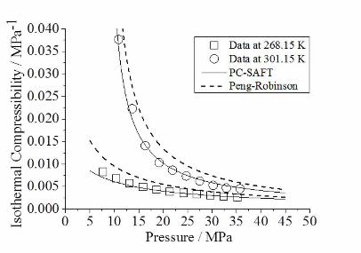
Figure 11 is a typical example of the improved capacity of the newly developed SAFT

equation of state in the prediction of the isothermal compressibility of multi-component

systems. Experimental data for derivative properties of complex mixtures are scarce in the

literature. Amongst what is available (Alsiyabi et al., 2012), the CO2-N2-CH4-H2 system was

selected due to it resembling candidate CO2 pipeline mixtures better. Figure 11 compares

predictions obtained from the Peng-Robinson and the newly developed PC-SAFT equations

of state, and PC-SAFT displays a notably superior average absolute deviation error of 5.3 %

against 33.2 % for the classical approach. It should be emphasized that no tuning to

isothermal compressibility data has been undertaken in the construction of any model. The

improved capacity of PC-SAFT is attributed more to the fact that the mathematical terms

resemble the physical interactions more closely, and less to the fact that PC-SAFT has

slightly more complex functional form and an extra adjustable parameter.

5. NEAR-FIELD MULTI -PHASE DISPERSION MODELLING

5.1 Turbulent Flow Calculations

Predictions were based on the solutions of the Favre-averaged, density-weighted forms of the

transport equations for mass, momentum, and total energy (internal energy plus kinetic

energy), as described below by equations 27, 28, and 29 respectively:

( ) 0ii

ut x

ρ ρ∂ ∂+ =

∂ ∂ (27)

( ) ( ) 0i i j i j uj

u u u p u u st xρ ρ ρ∂ ∂ ′′ ′′+ + + − =

∂ ∂ (28)

( ) 0i i ij t Ei i j

E SE p u u T s

t x x xτ µ

∂ ∂ ∂ ∂ + + − − − = ∂ ∂ ∂ ∂

(29)

Representation of the Reynolds stresses (i ju u′′ ′′ ), and hence the closure of this equation set,

was achieved via the k ε− turbulence model (Jones and Launder, 1972). Solutions of the

time-dependent, axisymmetric forms of the descriptive equations were obtained using a

modified version of an in-house general-purpose fluid dynamics code. Integration of the

equations employed a second-order accurate, upwind, finite-volume scheme in which the

transport equations were discretised following a conservative control-volume approach, with

values of the dependent variables being stored at the computational cell centres.

Approximation of the diffusion and source terms was undertaken using central differencing,

and an HLL (Harten et al., 1983), second-order accurate variant of Godunov’s method

applied with respect to the convective and pressure fluxes. The fully-explicit, time-accurate

method was a predictor-corrector procedure, where the predictor stage is spatially first-order,

and used to provide an intermediate solution at the half-time between time-steps. This is then

subsequently used at the corrector stage for the calculation of the second-order fluxes. A

further explanation of this algorithm can be found elsewhere (Falle, 1991).

The calculations also employed an adaptive finite-volume grid algorithm which uses a three-

dimensional rectangular mesh with grid adaption achieved by the successive overlaying of

refined layers of computational mesh. Figure 12 demonstrates this technique in a two-

dimensional planar calculation of the near-field of a sonic CO2

Wareing et al., 2013

release. Where there are steep

gradients of variable magnitudes such as at flow boundaries or discontinuities such as the

Mach disc, the mesh is more refined than in areas such as the free stream of the surrounding

fluid. The model to describe the fluid flow-field employed in this study was cast in an

axisymmetric geometry for the validatory calculations of jet releases. A full three-

dimensional scheme was applied to the crater calculations although the use of symmetry

boundaries aided a reduction in computational expense. A full description of the equations

solved is reported elsewhere ( )

Although the standard k-i model has been extensively used for the prediction of

incompressible flows, its performance is well known to be poor in the prediction of their

compressible counterparts. The model consistently over-predicts turbulence levels and hence

mixing due to compressible flows displaying an enhancement of turbulence dissipation. A

number of modifications to the standard k-i model have been proposed by various authors,

which include corrections to the constants in the turbulence energy dissipation rate equation

(Baz, 1992; Chen and Kim, 1987), and to the dissipation rate itself (Sarkar et al., 1991;

Zeman, 1990). Previous works by one of the present authors (Fairweather and Ranson, 2003,

2006) have indicated that for flows typical of those being studied here, the model proposed

by Sarkar et al. (1991) provides the most reliable predictions. This model specifies the total

dissipation as a function of a turbulent Mach number and was derived from the analysis of a

direct numerical simulation of the exact equations for the transport of the Reynolds stresses in

compressible flows. This approach was incorporated into the modelling described herein.

5.2 Non-ideal Equation of State

The Peng-Robinson equation of state (Peng and Robinson, 1976) is satisfactory for predicting

the gas-phase properties of CO2 1996, but when compared to that of Span and Wagner ( ), it is

not so for the condensed phase. Furthermore, it is not accurate for gas pressures below the

triple point and, in common with any single equation, it does not account for the discontinuity

in properties at the triple point. In particular, there is no latent heat of fusion.

Span and Wagner (1996) give a formula for the Helmholtz free energy that is valid for both

the gas and liquid phases above the triple point, but it does not take account of experimental

data below the triple point, nor does it give the properties of the solid. In addition, the

formula is too complicated to be used efficiently in a computational fluid dynamics code. A

composite equation of state was therefore constructed to determine the phase equilibrium and

transport properties for CO2

Wareing et al., 2013

. The inviscid version of the overall model is presented in detail

elsewhere ( ) and the method considered here is extended for the turbulent

closure of the fluid-flow equations detailed in the previous section. In this, the gas phase is

computed from the Peng-Robinson equation of state (Peng and Robinson, 1976), and the

liquid phase and saturation pressure are calculated from tabulated data generated with the

Span and Wagner (1996) equation of state and the best available source of thermodynamic

data for CO2

DIPPR, 2013

, the Design Institute for Physical Properties (DIPPR) 801 database, access to

which can be gained through the Knovel library ( ). To calculate the solid

density, the same approach as Witlox et al. (2009) is used, and expressed as:

31289.45 1.8325T kg mρ −= + (30)

again based on property information from the DIPPR 801 Database. From Liu (1984), the

sound speed in solid CO2 at atmospheric pressure and 296.35 K is 1600 m s-1

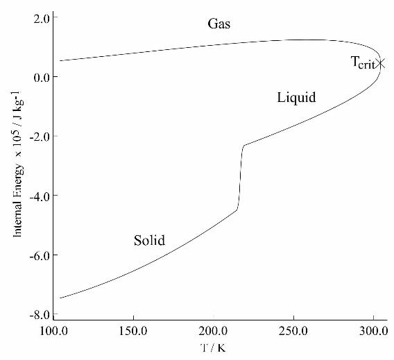
Figure 13 shows the predicted internal energy of the gas and condensed phases on the

saturation line. The transition from liquid to solid was smoothed over 4 K with a hyperbolic

tangent function centred on the triple point. This was done for computational reasons in order

to ensure the function and its differentials are smooth.

and it is

assumed that this is independent of temperature and pressure. Note that the results given

below are extremely insensitive to the solid density and sound speed. The saturation pressure

above and below the triple point is taken from Span and Wagner (1996).

Calculations of the thermodynamics in the pure CO2 system indicated that in this case, little

difference was observed between results obtained using the approach described above, and

that presented in Section 4. Hence, for the unique case of a pure CO2 release, the composite

non-ideal equation of state was used in the form of look-up tables to increase computational

efficiency. It will be essential to apply the more advanced equations of state such as PC-

SAFT when considering systems containing mixtures of CO2

with impurities.

5.3 Homogeneous Equilibrium and Relaxation Models

In an HEM, all phases are assumed to be in dynamic and thermodynamic equilibrium. Id est

they all move at the same velocity and have the same temperature. In addition, the pressure of

the CO2 vapour is assumed to be equal to the saturation pressure whenever the condensed

phase is present. The pressure of the condensed phase CO2 is assumed to be equal to the

combined pressure of CO2

The assumptions associated with the HEM are reasonable provided the CO

vapour and air (the total pressure).

2

Woolley et al., 2013

liquid droplets or

solid particles are sufficiently small. There are some indications that this may not be true, in

particular for test calculations in which the release is from a nozzle with a diameter of the

order of centimetres. Hence, the model was further developed as an HRM, in that a relaxation

time was introduced with respect to the transport of the dense phase. This has the effect of

numerically representing the time taken for the dense phase to attain dynamic equilibrium

with the fluid phase. Again, a full description of both the HEM and HRM can be found

elsewhere ( ).

5.4 Code Validation against CO2

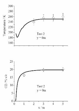
Figure 14 depicts centreline predictions of temperature and O

Release Data

2 molar concentration plotted

against experimental data for Test 2 at axial locations of 2, 3, 4, and 5 m. This test was

undertaken using the 6 mm nozzle, and predictions can be seen to be in good agreement with

observation. A slight over-prediction of temperature is observed in the very near-field,

leading to a similarly slight under-prediction further downstream. However, predictions

remain well within an acceptable range of experimental error. Again with reference to Figure

14, this over-prediction of temperature is translated into a slight over-prediction of O2

In addition, Figure 15 shows predictions of radial temperature profiles plotted against

experimental data for Test 8, performed by INERIS, at axial locations of 1, 2 and 5 m. The

model qualitatively and quantitatively captures the thermodynamic structure of the sonic

releases, and although there is a small discrepancy with the observed and predicted spreading

rates in the very near-field, calculations lie within the accepted error range of the

experimental data. Results obtained from calculations of two further tests, Tests 6 and 7 (not

shown), were seen to be of a similar level of agreement to Test 8. Further discussion

concentration, at an axial location of 1 m.

regarding this validation exercise, and the results obtained, can be found in Woolley et al.

(2013).

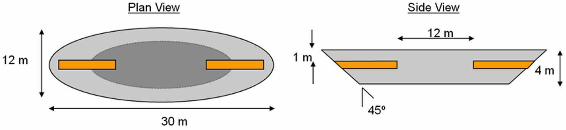
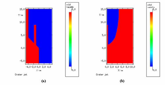
5.5 Crater Calculation Geometry and Sample Results

Figure 16 shows the chosen geometry of the crater formed after the pipeline guillotine

rupture. This geometry was chosen, based upon incident data for natural gas pipelines taken

from the literature (Kinsman and Lewis, 2002; McGillivray and Wilday, 2009).

This geometry was incorporated into a three-dimensional model for predicting the near-field

dispersion characteristics, and Figure 17 shows an example of such a set-up in which one

quarter of the crater has been modelled by applying appropriate symmetry boundaries. Figure

17 (a) depicts a cut along the centreline on the y-axis, which lies along the centre of the

release pipe at x=0. The z dimension represents the crater depth, and symmetry boundaries

are located at x=0 and y=15 m. Figure 17 (b) is looking down on to a plane in the x

dimension, bisecting the pipe at a depth of 1.5 m. The symmetric left boundary at x=0 can

also be seen to bisect the pipe. As previously mentioned, the uppermost boundary at y=15 m

is also symmetric, and represents the companion jet release in a symmetrical full-bore release

scenario.

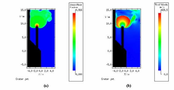
Figure 18 shows sample predictions of a typical release obtained from the application of this

crater geometry, with initial conditions (pressure, temperature, density, velocity, and phase

composition) provided by the pipe outflow model described earlier. The flow is modelled as a

steady state, using the predicted conditions at the pipeline orifice 30 seconds after the start of

the release, following the methodology proposed for modelling transient pipeline releases by

Carter (1991), and Bilio and Kinsman (1997). Dense-phase CO2 mass fraction and total

velocity predictions are presented, and the features of such a highly under-expanded jet can

be seen, including the formation of a Mach disc, and the acceleration of the flow to

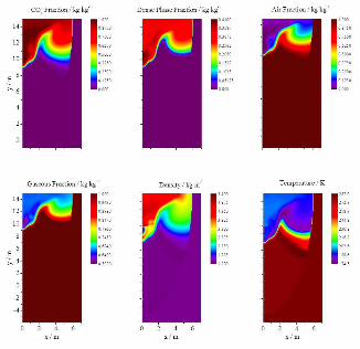
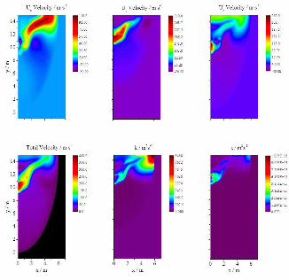
supersonic velocities. Figure 19 and Figure 20 depict predictions of the full-bore release on a

section located just above ground level and on a plane orthogonal to the z axis at 0.01 m.

Figure 19 shows mixture fractions of total CO2, solid CO2, air, and gas, and overall density

and temperature. Figure 20 shows the velocity components, total velocity, turbulence kinetic

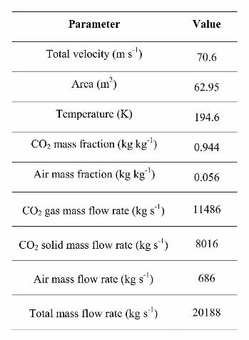
energy, and turbulence kinetic energy dissipation rate. To interface these results from the

near-field model with the far-field dispersion models, described below as FLACS and

ANSYS-CFX, equivalent point-source boundary conditions were calculated by integrating

the data shown in Figures 19 and 20 within an envelope defined by a CO2

These source terms were subsequently used for far-field dispersion calculations undertaken

by partners HSL and GexCon AS, and reported upon in Section 6.

concentration of

0.1%. The resulting integrated source values are as given in Table 5.

6. FAR-FIELD MULTI -PHASE DISPERSION MODELLING

Far-field modelling of the dispersion of two-phase (gaseous and particulate) CO2

ANSYS, 2011

was

undertaken using two different commercial computational fluid dynamic codes: FLACS

(GexCon AS, 2013); and ANSYS-CFX ( ). In both cases, the continuous gas-

phase was solved in the Eulerian reference frame, while a Lagrangian formulation was used

for the dispersed particle phase. In addition, both far-field models employed the same source

boundary conditions, where the CO2 jet conditions at the inlet plane were taken from the

near-field dispersion model outputs, as described above, which consisted of integrated planar

profiles of velocity, temperature, CO2

solid and gas concentration, turbulence kinetic energy

and turbulence dissipation rate. Distinct features of each of the individual codes are given

below.

6.1 ANSYS-CFX

The CFX dispersion model for two-phase CO2

ANSYS, 2011

releases used the Lagrangian particle-tracking

model in ANSYS-CFX version 14 ( ). The process of sublimation was

simulated using the standard evaporation model, with suitable Antoine equation coefficients

for solid CO2 sublimation. Drag between the CO2

Schiller and Naumann (1933

particles and the surrounding gas phase

was calculated using the drag model of ) combined with the

stochastic dispersion model of Gosman and Ioannides (1981) to account for turbulence

effects. Heat transfer between the gaseous and solid phases was modelled using the Ranz-

Marshall correlation (Ranz and Marshall, 1952) and turbulence effects in the gas phase were

modelled using the Shear-Stress Transport (SST) model of Menter (1994).

To account for the effects of ambient humidity, the modelled gas phase was composed of a

mixture of three components: dry air, CO2

Brown and Fletcher (2005

, and water vapour, each of which was treated as

an ideal gas. An additional dispersed-droplet Eulerian phase was used to account for

condensed water droplets, which were assumed to have the same velocity as the surrounding

gas phase. Source terms in the continuity and energy conservation equations were used to

model the process of water vapour condensation and evaporation. )

previously demonstrated a similar approach to the modelling of atmospheric plumes from

alumina refinery calciner stacks. It is useful to model humidity not only in terms of its effect

on the dispersion behaviour, but also to provide predictions of condensed water droplet

concentration, from which the plume visibility can be inferred. The visibility of the CO2

The computational grids used with CFX in the present work were unstructured, using both

tetrahedral and prism-shaped cells. Previous tests have shown that relatively fine grids are

needed to resolve the sublimation process in two-phase CO

plume has important practical implications for emergency planning and risk assessment.

2

The near-field dispersion model outputs do not currently include predictions of the CO

jets and therefore in excess of 3

million nodes were used in the CFX simulations presented here.

2

particle size, which is an important input for the Lagrangian two-phase dispersion model. The

size of the solid CO2 particles produced by dense-phase CO2 releases is uncertain, and it

cannot be measured reliably in large-scale releases. However, previous work has shown that

homogeneous equilibrium dispersion models provide reasonably good predictions of

temperatures and concentrations in dense-phase CO2

Dixon et al., 2012

jets produced by orifices up to 50 mm

in diameter ( ; Witlox et al., 2012). These models assume that the particles

have the same temperature and velocity as the surrounding gas phase, which implies that the

particles must be very small. Analysis of CO2 particle sizes by Hulsbosch-Dam et al. (2012)

has also suggested that their initial diameter once the jet has expanded to atmospheric

pressure should be in the range 1-20 たm. In the present work the CO2

At the far-field boundaries, logarithmic wind velocity profiles and turbulence levels were

specified using the approach described by Richards and Hoxey (

particles are assigned

an initial uniform diameter of 20 たm at the inlet plane, and their diameter subsequently

reduces as they sublimate.

1993). For the thermal

boundary conditions, it is assumed that the stability of the atmospheric boundary layer is

neutral.

Further information on the CFX dispersion model for two-phase CO2

2012

releases can be found

in the work of Dixon et al. ( ).

6.2 FLACS

In the current study, two-phase CO2

Ichard, 2012

dispersion phenomena in FLACS (GexCon AS, 2013)

are modelled using an Euler-Lagrangian method ( ). The numerical particles are

modelled as point-particles (Loth, 2000), with the particles considered incompressible, non-

reacting, and spherical in shape. Particle sizes are further represented by a uniform

distribution. The governing equations solved for the continuous gas phase are the

compressible form of Reynolds-averaged Navier-Stokes equations, where turbulence is

modelled using a standard k-i model (Launder and Spalding, 1974). A two-way coupling

between the continuous gas-phase and the dispersed particle-phase is established through

source terms in the mass, momentum, and energy equations (Peirano et al., 2006). In

addition, particle-turbulence interaction is accounted for by special source terms in the

turbulence kinetic energy and the dissipation rate of turbulence kinetic energy equations

(Mandø et al., 2009).

A simplified form of the original equation of Maxey and Riley (1983) is used for the particle

momentum equation, where the simplification is based on the analysis of Armenio and

Fiorotto (2001) for a wide range of particle-fluid density ratios. In the present particle

momentum equation, both the buoyancy force and the drag force were considered, while the

added-mass force and the Basset history force were ignored since they are negligibly small

when compared to the drag force (Armenio and Fiorotto, 2001). In addition, the pressure-

gradient force term was also omitted, since its influence is small in large particle-fluid density

ratio problems (Armenio and Fiorotto, 2001). The instantaneous fluid velocity seen by the

particle, which is an unknown parameter in the particle momentum equation, is modelled

through stochastic differential equations. A modified Langevin equation derived by Minier

and Peirano (2001) was used for this purpose.

Particle deposition and interaction with obstacles was modelled (Crowe, 2005), while

particle-particle interactions such as collisions, breakup and coalescence were not taken into

account. In addition, humidity effects were not considered in the present version of the

Lagrangian particle-tracking model.

The governing equations were solved on a staggered Cartesian grid using a finite-volume

method. The solver for both the continuous phase and the dispersed phase was second-order

accurate. A central-differencing scheme is used for the diffusive fluxes, while a hybrid

scheme with weighting between upwind and central-differences was employed for the

convective fluxes. Time-marching was carried out using an implicit backward-Euler scheme

and the discretized equations were solved using a BICGStab iterative method with the

SIMPLE pressure correction algorithm (Versteeg and Malalasekera, 2007). Readers are

referred to Ichard (2012) for further information concerning FLACS Lagrangian particle-

tracking model and its validation.

6.3 Implementation of Realistic Terrain and Boundary Conditions

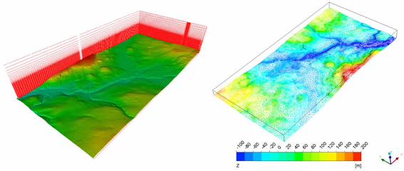
The realistic terrain employed was obtained from UK Ordnance Survey data and incorporated

into the FLACS and CFX models, as shown in Figure 21. The length and width of the domain

size in each case is 10 km and 5 km respectively. The FLACS domain extended to a height of

approximately 1 km, whilst a lesser height was used in CFX, which varied from 260 m to 610

m depending upon the location. The computational grids used in the two codes were very

different as FLACS employed a multi-block Cartesian mesh with 2.7 million grid points,

whilst CFX used an unstructured grid of 3.2 million nodes that was composed of mainly

tetrahedral cells, with prism-shaped cells along the solid boundaries.

For the dispersion model boundary conditions, the CO2 source from the crater was specified

using the conditions given in Table 5. For the turbulence source conditions in FLACS, a

relative turbulence intensity of 0.1985 and turbulence length scale of 0.034 m, obtained from

averaged k and ɂ values in Figure 20, were used. In both the FLACS and CFX models, the

CO2 particles were assigned an initial uniform diameter of 300 µm and 20 µm, respectively.

The likely size of particles produced in dense-phase CO2 releases is largely unknown,

certainly for releases of the scale considered here, as discussed earlier. In addition, the initial

temperature of the CO2 particles in the FLACS simulation was set to the sublimation

temperature of 194.25 K. For the upwind boundary condition, logarithmic cross-wind

velocity profiles were used with a reference speed of 2 m s-1 for the FLACS simulations and

5 m s-1 for the CFX simulations, at a reference height of 10 m. Both models assumed Pasquill

class type D (neutral) atmospheric stability and a ground roughness of 0.1 m, suitable for

rural roughness with low crops and occasional large obstacles. The ambient temperature was

283 K, and for a maximum depressurisation time of 200 seconds, the total mass discharge

predicted by the pipeline outflow model was approximately 2700 tonnes. Therefore, with

reference to the mass flow rate in Table 5, the release duration was approximately 138

seconds, and the FLACS simulations were performed for a release over this period using a

transient solver. Following the release cut-off, the dispersion calculations were simulated for

a further 400 seconds. In contrast, the CFX simulations were performed using a steady solver,

and the results therefore provide predictions assuming that the release was prolonged.

6.4 Results and Discussion

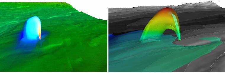
The predicted CO2 jet in the vicinity of the crater is shown in Figure 22 for the FLACS and

CFX models. Owing to the smaller particle-size used in the CFX simulations, it was found

that all of the particles sublimated within the airborne jet, and these particle trajectories are

shown in the right-hand plot of Figure 22. In contrast, the larger initial particle-size

prescribed in the FLACS simulations resulted in some solid-CO2 mass raining-out on to the

terrain. Towards the end of the FLACS simulation, it was recorded that approximately 20%

of the total mass discharged, at around 550 tonnes, had rained-out on the ground. This result

suggests that banks of solid CO2 might be formed in CO2

pipeline releases if particles with

diameters of the order 300 µm or larger are produced in the jet leaving the crater.

Figure 23 shows the steady-state cloud predicted by the CFX model. These predictions are

shown using three different CO2 mean concentration levels to define the edge of the cloud:

1%, 2% and 4% v/v. For these three cases, the cloud extends to approximately 5 km, 4 km,

and 2 km respectively. At low concentrations of 1% or 2%, CO2 is considered not harmful

but these concentrations may correlate to the extent of the visible cloud due to condensed

water vapour (i.e. mist). A concentration of 4% v/v CO2

1996

corresponds to the Immediately

Dangerous to Life and Health (IDLH) value recommended by NIOSH ( ). The CFX

results show that even with a wind speed of 5 m s-1, the presence of the terrain has a large

effect on the dispersion of the CO2

cloud, and rather than being blown downwind, the cloud

spreads mostly in the lateral directions, up and down the valley.

Figure 24 shows the CO2 cloud predicted by FLACS at various intervals in time. These are

after the beginning of the release, a little after the release cut-off, 100 seconds after the

release cut-off, and finally near the end of the simulation. Owing to the finite total mass

discharge, the CO2 cloud is notably smaller than that predicted by the steady-state release

CFX simulations. It can be observed from Figure 24(b) that the maximum CO2 concentration

almost reduces to half (45% v/v) a little after the release cut-off and gradually reduces with

time to reach 4% v/v near the end of the simulation (Figure 24(d)).

7. CONCLUSIONS

The process of simulating a hypothetical ‘realistic’ release from a buried 0.914 m (36 inch)

diameter, 217 km long pipeline has been demonstrated. Models for the pipeline outflow,

near-field and far-field dispersion have been integrated, along with suitable thermophysical

property models. A schematic representation of this integration is given as Figure 25. Results

from the outflow model have been used to specify inlet boundary conditions for the near-field

dispersion model, which in turn has provided inlet boundary conditions for the far-field

dispersion model. Where possible, the models have been validated against data available in

the open literature, and also using data generated by partners during the execution of the EC

FP7 CO2PipeHaz project.

The work has demonstrated that it is feasible, in principle, to simulate such industrially-

relevant flows. However, the computing resources required were found to be significant,

requiring of the order weeks of computing time for the full solution. The use of this type of

integrated modelling approach therefore appears unlikely to become widespread for routine

CO2

One of the limitations of the approach demonstrated here is that the models are integrated in a

linear fashion, with no feedback between them. This feedback could be particularly important

if low wind speeds were to be simulated. In the present near-field model, the flow entrained

into the crater was assumed to consist of ambient air, whereas under low wind-speed

conditions, the CO

pipeline risk assessment at present, if conducted upon standard workstation computers.

However, these models should be immediately useful for the investigation of particular

aspects of risk assessments. For instance, those where there are large differences in terrain

heights close to a pipeline route, and where the effect of the terrain on the dispersion

behaviour needs to be assessed in detail.

2 jet may fall to the ground near the crater and this flow could include very

high CO2

In the future, it would be useful to further validate this integrated modelling approach against

publicly-available datasets, particularly those involving releases of dense-phase CO

concentrations. The two-way coupling of the near- and far-field dispersion models

is not trivial, but it should be reasonably straightforward to apply the concentrations predicted

by the far-field model onto the near-field model boundaries, and for this process to be iterated

a number of times if required, to account for these effects.

2 from

buried pipelines. The present work has demonstrated that the size of the solid CO2 particles

released from a crater can have a significant effect upon the dispersion characteristics of the

release.

In view of the fact that most routine pipeline risk assessments will be carried out using

integral or other phenomenological models that assume dispersion over flat terrain, it would

be useful to use the models demonstrated here to determine under what set of conditions such

models might provide unreliable results. It should be possible to investigate this matter by

varying inputs (e.g. pipeline release rate, wind speed, terrain height differences) to the type of

models presented here to investigate under what combination of conditions the results deviate

significantly from those of more pragmatic modelling approaches.

Finally, from an emergency-planning perspective, it would be useful to further develop and

validate models that are able to predict the extent of the visible CO2 plume, as well as its

extent in terms of its instantaneous hazardous CO2

concentrations. Under typical humid

northern European climatic conditions, a full-bore pipeline rupture may produce an optically-

dense cloud that extends many kilometres.

8. NOMENCLATURE

Roman letters: Greek letters: A Helmholtz free energy α dynamic vapour quality d diameter ρ density e internal energy τ relaxation time E total energy ijτ shear stress

wf Fanning friction factor

p pressure s source term Subscripts: T temperature t time c critical u velocity eq equilibrium v volume i spatial indice x spatial location in inlet j spatial indice Superscripts: ml meta-stable liquid s at saturation A Reynolds average sv saturated vapour

A Favre average t turbulent A′′ fluctuating component

9. ACKNOWLEDGEMENTS

The research leading to the results described in this paper has received funding from the

European Union 7th Framework Programme FP7-ENERGY-2009-1 under grant agreement

number 241346. The paper reflects only the authors’ views and the European Union is not

liable for any use that may be made of the information contained herein.

One of the authors, S.E. Gant (HSL), was additionally funded by the UK Health and Safety

Executive. The contents of this paper, including any opinions and/or conclusions expressed,

are those of the authors alone and do not necessarily reflect HSE policy.

10. REFERENCES

Alsiyabi, I., Chapoy, A., Tohidi, B., 2012. Effects of impurities on speed of sound and

isothermal compressibility of CO2-rich systems, 3rd International Forum on the

Transportation of CO2

Angielczyk, W., Bartosiewicz, Y., Butrymowicz, D., Seynhaeve, J.-M., 2010. 1-D Modeling

Of Supersonic Carbon Dioxide Two-Phase Flow Through Ejector Motive Nozzle,

International Refrigeration and Air Conditioning Conference. 12-15 July, Purdue University,

Lafayette, USA, p. 2362.

by Pipeline, Gateshead, UK.

ANSYS, 2011. ANSYS CFX-Solver Theory Guide - Release 14.0.

Armenio, V., Fiorotto, V., 2001. The Importance of the Forces Acting on Particles in

Turbulent Flows. Phys. Fluids 13(8), 2437-2440.

Baz, A.M.E., 1992. Modelling Compressibility Effects on Free Turbulent Shear Flows, 5th

Biennial Colloquium on Computational Fluid Dynamics, UMIST.

Bilio, M., Kinsman, P., 1997. MISHAP - HSE’s pipeline risk assessment methodology. Pipes

and Pipelines International July-August, 5-12.

Brown, G.J., Fletcher, D.F., 2005. CFD Prediction of Odour Dispersion and Plume Visibility

for Alumina Refinery Calciner Stacks. Process Saf. Environ. 83(B3), 231-241.

Brown, S., Martynov, S., Mahgerefteh, H., Proust, C., 2013. A Homogeneous Equilibrium

Relaxation Flow Model for the Full Bore Rupture of Dense Phase CO2

Carter, D.A., 1991. Aspects of risk assessment for hazardous pipelines containing flammable

substances. J. Loss Prevent. Proc. 4(2), 68-72.

Pipelines. Int. J.

Greenh. Gas Con. 17, 349-356.

Chen, N.H., 1979. An Explicit Equation for Friction Factor in Pipe. Ind. Eng. Chem. Fun.

18(3), 296-297.

Chen, Y.S., Kim, S.W., 1987. Computation of Turbulent Flows Using an Extended k-ε

Turbulence Closure Model. Document number CR-179204.

CO2PipeHaz, 2009. Quantitative Failure Consequence Hazard Assessment for Next

Generation CO2

Cowley, L.T., Tam, V.H.Y., 1988. Consequences of Pressurised LPG Releases: The Isle of

Grain Full Scale Experiments, GASTECH 88 - 13

Pipelines: The Missing Link. accessed: 12/08/13, CO2PipeHaz Project

Website. http://www.co2pipehaz.eu/

th

Crowe, C.T., 2005. Multiphase Flow Handbook. CRC Press Inc., Bosa Roca, USA.

International LNG/LPG Conference,

Kuala Lumpur.

Diamantonis, N., Economou, I.G., 2011. Evaluation of Statistical Associating Fluid Theory

(SAFT) and Perturbed Chain-SAFT Equations of State for the Calculation of

Thermodynamic Derivative Properties of Fluids Related to Carbon Capture and

Sequestration. Energ. Fuel. 25(7), 3334-3343.

Diamantonis, N.I., Boulougouris, G.C., Mansoor, E., Tsangaris, D.M., Economou, I.G., 2013.

Evaluation of Cubic, SAFT, and PC-SAFT Equations of State for the Vapor-liquid

Equilibrium Modeling of CO2

Diamantonis, N.I., Economou, I.G., 2012. Modeling the Phase Equilibria of a H

Mixtures with other Gases. Ind. Eng. Chem. Res. 52(10),

3933-3942.

2O-CO2

Imperial College London, 2013. DIPPR 801 Database. accessed: 12/08/13.

http://www.aiche.org/dippr/

Mixture with PC-SAFT and tPC-PSAFT Equations of State. Mol. Phys. 110, 1205-1212.

Dixon, C.M., Gant, S.E., Obiorah, C., Bilio, M., 2012. Validation of Dispersion Models for

High Pressure Carbon Dioxide Releases, IChemE Hazards XXIII. IChemE, Southport, UK,

pp. 153-163.

Fairweather, M., Falle, S.A.E.G., Woolley, R.M., 2011. A Two-Dimensional, Axisymmetric

Computational Fluid Dynamic Code Capable of Predicting the Near-Field Structure of High

Pressure Releases of Supercritical and Multi-Phase Carbon Dioxide, Deliverable 1.4.1

CO2PipeHaz project. EU Grant Agreement 241346, http://www.co2pipehaz.eu/.

Fairweather, M., Ranson, K.R., 2003. Modelling of Underexpanded Jets Using

Compressibility-Corrected, k-ε Turbulence Models, in: Hanjalic, K., Nagano, Y., Tummers,

M. (Eds.), Turbulence, Heat and Mass Transfer 4. Begell House, Inc., pp. 649-656.

Fairweather, M., Ranson, K.R., 2006. Prediction of Underexpanded Jets Using

Compressibility-Corrected, Two-Equation Turbulence Models. Prog. Comput. Fluid Dy.

6(1,2,3), 122-128.

Falle, S.A.E.G., 1991. Self-Similar Jets. Mon. Not. R. Astron. Soc. 250, 581-596.

GexCon AS, 2013. FLACS v10.0 User's Manual. accessed: 12/08/13. http://www.flacs.com

Gosman, A.D., Ioannides, E., 1981. Aspects of Computer Simulation of Liquid Fuelled

Combustors. J. Energy 7(6), 482-490.

Harten, A., Lax, P.D., Leer, B.v., 1983. On Upstream Differencing and Godunov-Type

Schemes for Hyperbolic Conservation Laws. Society for Industrial and Applied Mathematics

Review 25(1), 35-61.

Ichard, M., 2012. Numerical Computations of Pressurized Liquefied Gas Releases Into the

Atmosphere, Ph.D. Thesis, Department of Physics and Technology, University of Bergen,

ISBN: 978-82-308-2010-0.

Jamois, D., Proust, C., Hebrard, J., Gentilhomme, O., 2013. La sécurité du captage et du

stockage du CO2

Jones, W.P., Launder, B.E., 1972. The Prediction of Laminarization with a Two-Equation

Model of Turbulence. Int. J. Heat Mass Tran. 15, 301-314.

: un défi pour les industries de l’énergie Récents Progrès en Génie des

Procédés 104. ISBN: 978-2-910239-78-7.

Kinsman, P., Lewis, J., 2002. Report on a Second Study of Pipeline Accidents Using the

Health and Safety Executive’s Risk Assessment Programs MISHAP and PIPERS. HSE

Books.

Launder, B.E., Spalding, D.B., 1974. The Numerical Computation of Turbulent Flows.

Computer Methods in Applied Mechanics and Engineering 3, 269-289.

LeVeque, R.J., 2002. Finite Volume Methods for Hyperbolic Problems. Cambridge

University Press, Cambridge.

Liu, L.-G., 1984. Compression and Phase Behavior of Solid CO2

Loth, E., 2000. Numerical Approaches for Motion of Dispersed Particles, Droplets and

Bubbles. Prog. Energ. Combust. 26(3), 161-223.

to Half a Megabar. Earth

Planet. Sc. Lett. 71(1), 104-110.

Mahgerefteh, H., Brown, S., Denton, G., 2012a. Modelling the Impact of Stream Impurities

on Ductile Fractures in CO2

Mahgerefteh, H., Brown, S., Martynov, S., 2012b. A study of the effects of friction, heat

transfer, and stream impurities on the decompression behavior in CO

Pipelines. Chem. Eng. Sci. 74(1), 200-210.

2

Mahgerefteh, H., Saha, P., Economou, I.G., 1999. Fast Numerical Simulation for Full Bore

Rupture of Pressurized Pipelines. AIChE Journal 45(6), 1191-1201.

pipelines. Greenhouse

Gases: Science and Technology 2, 369-379.

Mahgerefteh, H., Wong, S.M.A., 1999. A Numerical Blowdown Simulation Incorporating

Cubic Equations of State. Comput. Chem. Eng. 23(9), 1309-1317.

Mandø, M., Lightstone, M.F., Rosendahl, L., Yin, C., Sørensen, H., 2009. Turbulence

Modulation in Dilute Particle-Laden Flow. Int. J. Heat Fluid Fl. 30(2), 331-338.

Martynov, S., 2013. A Validated Heterogeneous Discharge Model, Deliverable 1.3.3

CO2PipeHaz project. EU Grant Agreement 241346, http://www.co2pipehaz.eu/.

Maxey, M.R., Riley, J.J., 1983. Equation of Motion for a Small Rigid Sphere in a

Nonuniform Flow. Phys. Fluids 26(4), 883-889.

McGillivray, A., Wilday, J., 2009. Comparison of Risks from Carbon Dioxide and Natural

Gas Pipelines.

Menter, F.R., 1994. Two-Equation Eddy-Viscosity Turbulence Models for Engineering

Applications. AIAA Journal 32(8), 1598-1605.

Minier, J.-P., Peirano, E., 2001. The PDF Approach to Turbulent Polydispersed Two-Phase

Flows. Phys. Rep. 352(9), 1-214.

Munkejord, S.T., Jakobsen, J.P., Austegard, A., Molnvik, M.J., 2010. Thermo- and fluid-

dynamical modelling of two-phase multi-component carbon dioxide mixtures. Int. J. Greenh.

Gas Con. 4(4), 589-596.

Narasimhamurthy, V.D., Skjold, T., Gant, S.E., 2013. On the Validation Studies of Two-

Phase Models in FLACS and CFX, Deliverable 1.5.4 CO2PipeHaz project. EU Grant

Agreement 241346, http://www.co2pipehaz.eu/.

National Institute for Occupational Safety and Health, 1996. Documentation for Immediately

Dangerous to Life or Health Concentrations (IDLHs) for Carbon Dioxide. accessed.

http://www.cdc.gov/niosh/idlh/124389.html

Peirano, E., Chibbaro, S., Pozorski, J., Minier, J.-P., 2006. Mean-Field/PDF Numerical

Approach For Polydispersed Turbulent Two-phase Flows. Prog. Energ. Combust. 32(3), 315-

371.

Peng, D.-Y., Robinson, D.B., 1976. A New Two-Constant Equation of State. Ind. Eng. Chem.

Fun. 15(1), 59-64.

Popescu, M., 2009. Modeling of Fluid Dynamics Interacting with Ductile Fraction

Propagation in High Pressure Pipeline. Acta Mech. Sinica 25(3), 311-318.

Ranz, W.E., Marshall, W.R., 1952. Evaporation from Drops. Part I. Chem. Eng. Prog. 48,

141-146.

Richards, P.J., Hoxey, R.P., 1993. Appropriate Boundary Conditions for Computational

Wind Engineering Models using the k-i Turbulence Model. J. Wind Eng. Ind. Aerod.

46/47(1), 145-153.

Richardson, S.M., Saville, G., 1996. Isle of Grain Pipeline Depressurisation Tests - OTH 94

441. HSE Books.

Sarkar, S., Erlebacher, G., Hussaini, M.Y., Kreiss, H.O., 1991. The Analysis and Modelling

of Dilatational Terms in Compressible Turbulence. J. Fluid Mech. 227(1), 473-493.

Schiller, L., Naumann, A.Z., 1933. Über die grundlegenden Berechnungen bei der

Schwerkraftaufbereitung. Z. Ver. Dtsch. Ing. 77(12), 318-320.

Soave, G., 1972. Equilibrium Constants from a Modified Redlich-Kwong Equation of State.

Chem. Eng. Sci. 27(6), 1197-1203.

Span, R., Wagner, W., 1996. A New Equation of State for Carbon Dioxide Covering the

Fluid Region from the Triple-Point Temperature to 1100 K at Pressures up to 800 MPa. J.

Phys. Chem. Ref. Data 25(6), 1509-1596.

Ordnance Survey, 2013. Ordnance Survey Land and Height Products. accessed: 12/08/13.

http://www.ordnancesurvey.co.uk/business-and-government/products/land-and-height-

products.html

Tsangaris, D.M., Boulougouris, G., Diamantonis, N.I., Economou, I.G., 2013. Physical

Properties Manual, Deliverable 1.2.6 CO2PipeHaz project. EU Grant Agreement 241346,

http://www.co2pipehaz.eu/.

Versteeg, H.K., Malalasekera, W., 2007. An Introduction to Computational Fluid Dynamics

The Finite Volume Method. Pearson Education Ltd.

Wareing, C.J., Woolley, R.M., Fairweather, M., Falle, S.A.E.G., 2013. A Composite

Equation of State for the Modelling of Sonic Carbon Dioxide Jets. AICheE Journal. DOI:

10.1002/aic.14102.

Webber, D.M., Fannelop, T.K., Witlox, H.W.M., 1999. Source Terms for Two-Phase Flow in

Long Pipelines Following an Accidental Breach, International Conference and Workshop on

Modeling the Consequences of Accidental Releases of Hazardous Materials. AIChE, San

Francisco, USA, pp. 145-168.

Witlox, H.W.M., Harper, M., Oke, A., 2009. Modelling of Discharge and Atmospheric

Dispersion for Carbon Dioxide Releases. J. Loss Prevent. Proc. 22(6), 795-802.

Witlox, H.W.M., Harper, M., Oke, A., 2012. Phast Validation of Discharge and Atmospheric

Dispersion for Carbon Dioxide Releases, Proceedings of the 15th Annual Symposium, Mary

Kay O’Connor Process Safety Centre, Texas A&M University, College Station, Texas, USA.

Woolley, R.M., Fairweather, M., Wareing, C.J., Falle, S.A.E.G., Proust, C., Hebrard, J.,

Jamois, D., 2013. Experimental Measurement and Reynolds-Averaged Navier-Stokes

Modelling of the Near-Field Structure of Multi-phase CO2

Zeman, O., 1990. Dilational Dissipation: The Concept and Application in Modeling

Compressible Mixing Layers. Phys. Fluids A-Fluid 2(2), 178-188.

Jet Releases. Int. J. Greenh. Gas

Con. 18, 139-149.

11. FIGURE CAPTIONS

Figure 1. Schematic diagram of the INERIS CO2

Figure 2. Schematic of the experimental rig main vessel and discharge pipe, with

illustratory photographs of valves and the discharge orifice.

release test rig including sensor

configuration.

Figure 3. Pressure vessel internal instrumentation.

Figure 4. Schematic of the orifice flange.

Figure 5. Schematic representation of the use of a subgrid to model the flow through a

small diameter puncture at the end of a pipe.

Figure 6. Elevation variation along pipeline route.

Figure 7. Upstream section, predicted release pressure, plotted against time for cases

with and without inclination.

Figure 8. Downstream section, predicted release pressure, plotted against time for cases

with and without inclination.

Figure 9. Total predicted mass discharge rate plotted against time for cases with and

without inclination.

Figure 10. Graphical representation of SAFT equation of state components.

Figure 11. Predictions and data of the isothermal compressibility of a quaternary CO2

Alsiyabi et

al. (2012

-

containing system plotted against pressure. Experimental data from

).

Figure 12. Adaptive mesh refinement grid mapped onto mean velocity predictions in the

region of a Mach disc.

Figure 13. CO2

Figure 14. Axial temperature and O

internal energy predictions on the saturation line obtained using the

composite equation of state, showing gaseous and dense phases.

2 mole fraction predictions plotted against

experimental data (symbols) for Tests 2.

Figure 15. Radial temperature profiles of Test 8 at axial distances of 1, 2 and 5 m (lines –

predictions, symbols – data).

Figure 16. Schematic of modelled crater shape and dimensions.

Figure 17. Sample three-dimensional geometry of a typical full-bore guillotine rupture

into an elliptic crater. (a) View at x=0 depicting the crater length, and (b) view

at z=0 depicting the crater plan.

Figure 18. Sample three-dimensional model predictions of a typical full-bore guillotine

rupture into a crater. (a) Dense-phase CO2

Figure 19. Near-field model predictions observed on a cross-sectional plane above the

crater just above ground level.

mass fraction, and (b) total

velocity.

Figure 20. Near-field model predictions observed on a cross-sectional plane above the

crater just above ground level.

Figure 21. Terrain data depicting grid methodologies, and coloured according to height

topography, loaded in FLACS (left) and CFX (right).

Figure 22. Predicted CO2

Figure 23. CFX predicted steady-state CO

jet in the vicinity of the crater using FLACS (left) and CFX

(right).

2 cloud, defined using three different mean

CO2

Figure 24. Snapshots of the CO

concentrations: 1% v/v (left); 2% v/v (middle); 4% v/v (right), and

coloured according to the distance from the crater source.

2 cloud at different time intervals, predicted by the

FLACS model at (a) t = 10 s; (b) t = 150 s; (c) t = 240 s; and (d) t = 540 s.

Here FMOLE (v/v) corresponds to volume fraction of CO2

Figure 25. Schematic representation of the thermo-physical modelling strategy.

.

12. TABLE CAPTIONS

Table 1. Parameters of the experimental releases.

Table 2. Discharge properties predicted using various equations of state in comparison with the measured values for Test 2 (Table 1).

Table 3. Discharge properties predicted using various equations of state in comparison with the measured values for Test 8 (Table 1).

Table 4. Derivative properties useful in the current work.

Table 5. Far-field source terms integrated from near-field calculations