This article was downloaded by: [York University Libraries] On: 12 August 2014, At: 05:41 Publisher: Taylor & Francis Informa Ltd Registered in England and Wales Registered Number: 1072954 Registered office: Mortimer House, 37-41 Mortimer Street, London W1T 3JH, UK Click for updates International Journal of Systems Science Publication details, including instructions for authors and subscription information: http://www.tandfonline.com/loi/tsys20 An integrated supply chain model for new products with imprecise production and supply under scenario dependent fuzzy random demand Lokesh Nagar a , Pankaj Dutta a & Karuna Jain a a Shailesh J. Mehta School of Management, Indian Institute of Technology, Bombay, Mumbai, India Published online: 20 Dec 2012. To cite this article: Lokesh Nagar, Pankaj Dutta & Karuna Jain (2014) An integrated supply chain model for new products with imprecise production and supply under scenario dependent fuzzy random demand, International Journal of Systems Science, 45:5, 873-887, DOI: 10.1080/00207721.2012.742594 To link to this article: http://dx.doi.org/10.1080/00207721.2012.742594 PLEASE SCROLL DOWN FOR ARTICLE Taylor & Francis makes every effort to ensure the accuracy of all the information (the “Content”) contained in the publications on our platform. However, Taylor & Francis, our agents, and our licensors make no representations or warranties whatsoever as to the accuracy, completeness, or suitability for any purpose of the Content. Any opinions and views expressed in this publication are the opinions and views of the authors, and are not the views of or endorsed by Taylor & Francis. The accuracy of the Content should not be relied upon and should be independently verified with primary sources of information. Taylor and Francis shall not be liable for any losses, actions, claims, proceedings, demands, costs, expenses, damages, and other liabilities whatsoever or howsoever caused arising directly or indirectly in connection with, in relation to or arising out of the use of the Content. This article may be used for research, teaching, and private study purposes. Any substantial or systematic reproduction, redistribution, reselling, loan, sub-licensing, systematic supply, or distribution in any form to anyone is expressly forbidden. Terms & Conditions of access and use can be found at http:// www.tandfonline.com/page/terms-and-conditions
Transcript
This article was downloaded by: [York University Libraries]On: 12 August 2014, At: 05:41Publisher: Taylor & FrancisInforma Ltd Registered in England and Wales Registered Number: 1072954 Registered office: Mortimer House,37-41 Mortimer Street, London W1T 3JH, UK
Click for updates
International Journal of Systems SciencePublication details, including instructions for authors and subscription information:http://www.tandfonline.com/loi/tsys20
An integrated supply chain model for new productswith imprecise production and supply under scenariodependent fuzzy random demandLokesh Nagara, Pankaj Duttaa & Karuna Jaina
a Shailesh J. Mehta School of Management, Indian Institute of Technology, Bombay, Mumbai,IndiaPublished online: 20 Dec 2012.
To cite this article: Lokesh Nagar, Pankaj Dutta & Karuna Jain (2014) An integrated supply chain model for new products withimprecise production and supply under scenario dependent fuzzy random demand, International Journal of Systems Science,45:5, 873-887, DOI: 10.1080/00207721.2012.742594
To link to this article: http://dx.doi.org/10.1080/00207721.2012.742594
PLEASE SCROLL DOWN FOR ARTICLE
Taylor & Francis makes every effort to ensure the accuracy of all the information (the “Content”) containedin the publications on our platform. However, Taylor & Francis, our agents, and our licensors make norepresentations or warranties whatsoever as to the accuracy, completeness, or suitability for any purpose of theContent. Any opinions and views expressed in this publication are the opinions and views of the authors, andare not the views of or endorsed by Taylor & Francis. The accuracy of the Content should not be relied upon andshould be independently verified with primary sources of information. Taylor and Francis shall not be liable forany losses, actions, claims, proceedings, demands, costs, expenses, damages, and other liabilities whatsoeveror howsoever caused arising directly or indirectly in connection with, in relation to or arising out of the use ofthe Content.
This article may be used for research, teaching, and private study purposes. Any substantial or systematicreproduction, redistribution, reselling, loan, sub-licensing, systematic supply, or distribution in anyform to anyone is expressly forbidden. Terms & Conditions of access and use can be found at http://www.tandfonline.com/page/terms-and-conditions
International Journal of Systems Science, 2014Vol. 45, No. 5, 873–887, http://dx.doi.org/10.1080/00207721.2012.742594
An integrated supply chain model for new products with imprecise productionand supply under scenario dependent fuzzy random demand
Lokesh Nagar, Pankaj Dutta∗ and Karuna Jain∗
Shailesh J. Mehta School of Management, Indian Institute of Technology, Bombay, Mumbai, India
(Received 24 May 2011; final version received 2 October 2012)
In the present day business scenario, instant changes in market demand, different source of materials and manufacturingtechnologies force many companies to change their supply chain planning in order to tackle the real-world uncertainty. Thepurpose of this paper is to develop a multi-objective two-stage stochastic programming supply chain model that incorporatesimprecise production rate and supplier capacity under scenario dependent fuzzy random demand associated with newproduct supply chains. The objectives are to maximise the supply chain profit, achieve desired service level and minimisefinancial risk. The proposed model allows simultaneous determination of optimum supply chain design, procurement andproduction quantities across the different plants, and trade-offs between inventory and transportation modes for both inboundand outbound logistics. Analogous to chance constraints, we have used the possibility measure to quantify the demanduncertainties and the model is solved using fuzzy linear programming approach. An illustration is presented to demonstratethe effectiveness of the proposed model. Sensitivity analysis is performed for maximisation of the supply chain profit withrespect to different confidence level of service, risk and possibility measure. It is found that when one considers the servicelevel and risk as robustness measure the variability in profit reduces.
Keywords: supply chain management; new products; two-stage stochastic programming; fuzzy random demand; possibilitymeasure
1. Introduction
Supply chain management is concerned with the coordina-tion and integration of key business activities undertaken byan enterprise, from the procurement of raw materials to thedistribution of the final products to the customer. New prod-uct introductions are vital to the growth of the corporaterevenues in both manufacturing and service industries. Infact, shortened life cycles are caused by fast changing con-sumer preferences and rapid rate of innovation especiallyin the high technology, consumer electronics and personalcomputers industries. Therefore, supply chain planning(SCP) for new products is challenging task for supplychain managers. But there are very few studies reportedin the literature addressing supply chain decision problemsrelated to new product supply chains (Ishii, Takahashi, andMuramatsu 1988; Butler, Ammons, and Sokol 2003; Gaon-akar and Viswanadham 2003). Further, there are hardly anymodels available that combine both the strategic and tacticalplanning (Dogan and Goetschalckx 1999; Santoso, Ahmed,Goetschalckx, and Shapiro 2005). Gupta and Maranas(2003) have developed a two-stage stochastic programmingmodel for SCP considering demand uncertainty. Productiondecisions are taken as first-stage decisions whereas logisticsdecisions are taken as second-stage decision variables. Itis reported that such integrated models provide several
advantages, especially for new product supply chain (Nagarand Jain 2008). The present work considers an integratedsupply chain decision problem over the life cycle of a newproduct combining strategic and tactical decisions in atwo-stage decision-making framework under uncertainty.
It is reported that traditional deterministic optimisationmodels are not suitable for capturing the dynamic behaviourof most real-world applications (Escudero, Galindo,Garcia, Gomez, and Sabau 1999; Min and Zhou 2002,Santoso et al. 2005). The SCP for new products becomesmore challenging when some parameters such as demand,resource availability and production processing time areeither uncertain or imprecise because some information iseither incomplete or inaccessible. Fuzzy set theory givesa strong mathematical structure to capture such impreciseor linguistic terms and to model a real decision-makingproblem.Wang and Shu (2005) have presented a fuzzysupply chain model by combining possibility theory andgenetic algorithm approach to provide an alternative frame-work to handle supply chain uncertainties.Petrovic, Xie,Burnham, and Petrovic (2008) have considered a singleproduct inventory control in a distribution supply chainin presence of fuzzy customer demand. Aliev, Fazlollahi,Guirimov, and Aliev. (2007) have developed a fuzzy inte-grated multi-period and multi-item production-distribution
model in supply chain context and solved using geneticalgorithms. Torabi and Hassini (2008) have presented aninteractive fuzzy possibilistic programming approach formultiple objective supply chain master planning. Liang(2008) has developed a fuzzy multi-objective linear pro-gramming (LP) model with piecewise linear membershipfunction to solve integrated multi-product and multi-timeperiod production distribution planning problems withfuzzy objectives. Peidro, Mula, Poler, and Verdegay (2009)have proposed a fuzzy mixed integer LP model for supplychain under supply, demand and process uncertainties.
Decision-making environment of supply chain plan-ning for new products is full of uncertainties arising fromrandomness and/or fuzziness of certain input parameterswhich warrants modelling under uncertainty. There aremany supply chain models that incorporate fuzzy demand(e.g. Petrovic, Roy, and Petrovic 1999; Chen and Lee 2004;Xie, Petrovic, and Burnham 2006; Chen, Lin, and Huang2006; Xu and Zhai 2008). One of the drawbacks of thesemodels is that the stochastic variation of demand is notreflected in these models. This work presents an integratedSCP problem for new products with scenario dependentfuzzy random demand that captures both fuzzy perceptionand random behaviour of customer demand in a singleoptimisation setting.
In this paper, we present a multiple objective two-stagestochastic programming supply chain model in a mixedfuzzy stochastic environment considering uncertain de-mand, production rate and supplier capacity. The demanduncertainty is covered through the scenario based fuzzyrandom approach. We consider three objectives: maximi-sation of profit, achieving desired service level and min-imising risk. In Section 2, we develop an integrated modelfor new product supply chain in a mixed fuzzy stochasticenvironment. In Section 3, a detailed solution procedureusing fuzzy LP is presented. The model is illustrated witha numerical example in Section 4 and finally, conclusionsare presented in Section 5.
2. Integrated model for new product supply chains
2.1. Problem description and assumptions
We consider a supply chain network consists of differentsuppliers able to supply different parts, single stage parallellines manufacturing facilities having limited production ca-pacities and two-stage distribution network. The differentmanufacturing and distribution facilities are connected ge-ographically by transportation channels. Selection of trans-portation mode between the facilities is driven by the trans-portation cost, cycle and pipeline inventory costs. The fixedcosts are employed for opening and closing of productionlines and distribution centres. For new product it is moreimportant to consider the service level and financial riskassociated with uncertain demand. Therefore, it is proposedto develop an integrated supply chain model with different
conflicting objective functions, namely, maximisation of ex-pected supply chain profit, achieving desired service leveland minimising risk associate with the profit, which givesthe decision-maker (DM) a set of optimal solutions to findthe best supply chain design and plans.
For new product supply chain, optimising a multi-product and multi-period modelling framework is verycomplex. In such cases, a two-stage distribution networkplays a vital role in getting a solution to the model. In thisapproach decision variables of a problem under uncertaintyare partitioned into two sets.
First-stage design variables such as plant location,processing line per location, raw material procurement,capacity utilisation and production are modelled as de-sign decisions, which need to be decided prior to demandrealisation.
Second-stage control variables such as such as inven-tory, shortage and supply of finished product to customerare modelled as control variables, which can be fine-tunedafter realisation of the actual demand. Figure 1 depicts theintegrated supply chain network with design and controlvariables in different stages.
Assumptions used in the problem formulation are asfollows:
• The fixed costs are employed for opening and closingof production lines and distribution centres. Thesecosts are the initial installations cost which are onetime cost and other fixed costs are assumed to be onper period basis irrespective of production quantity.
• The inventory costs are considered at warehouse levelfrom one period to another period.
• The transportation mode selection is determined onthe basis of total logistics cost.
• The demand uncertainty is covered with uniqueapproach of integrating scenario information withfuzzy random variable. For new product supplychain, the uncertain demand could more easily bedescribed as possible scenarios with the help ofindustry experts. When the expert’s opinions arelinguistic or imprecise in nature, these scenariovalues are treated as fuzzy numbers and appropri-ate triangular distribution is assigned. Stochasticvariation is present due to difficulty to predict withprecision occurrence of linguistic terms or imprecisedata (Puri and Ralescu 1986; Messina and Mitra1997; Dutta, Chakraborty, and Roy 2005; Xu andLiu 2008; Hu, Zheng, Xu, Ji, and Guo 2010; Xuand Zhou 2011). Figure 2 depicts the triangulardistributed fuzzy demand Djpmzi
based on the threeprominent data: most pessimistic value D
pjpmzi
, mostpossible value Dm
jpmzi, and the most optimistic value
Dojpmzi
(Dutta, Chakraborty, and Roy 2007).
Dow
nloa
ded
by [
Yor
k U
nive
rsity
Lib
rari
es]
at 0
5:41
12
Aug
ust 2
014
International Journal of Systems Science 875
Warehouse
Warehouse
Customer
Customer
Stage 1- Design variables: Plantlocation, processing line per location,raw material procurement, capacity
utilization and production
Stage 2- Control variables: Inventory, shortage andsupply of finished product to customer
Objectives: Maximize profit, achieve desiredservice level, and minimize financial risk
Plant
Plant
DistributionCenter
CustomerWarehouse
Supplier
Supplier
Supplier
DistributionCenter
Figure 1. Two-stage supply chain network.
• The supplier capacity and product processing timeare considered as imprecise in nature with linearmemberships function and shown in Figure 3.
2.2. Notations
The notations used in the proposed supply chain model arepresented in Tables 1 and 2.
2.3. The model
In order to develop the integrated SCP model for new prod-ucts under fuzzy-stochastic environment, we consider threedifferent conflicting quantitative objectives. The first objec-tive function is maximisation of expected profit consideringdifferent cost components, whereas the second objective isto control the service level in each period and in each sce-nario and third, minimising risk associated with the profitirrespective of scenarios.
Objective 1: Maximise the expected supply chain profit. Theexpected supply chain profit (ESCP) can be computed con-sidering all the cost components, i.e. opening and closingcosts of facilities (plants and warehouses), raw material pro-curement cost, manufacturing/production cost, transporta-tion cost (inbound and outbound) and inventory carrying
Figure 2. Triangular fuzzy demand.
cost. Then the ESCP (revenue − all the relevant costs) iscomputed as
ESCP =∑
wjplmzi
QwjplmziSPjpmPzi
−∑oim
(FC oimYoim + PI oimY1oim + PDoimY2oim)
−∑wm
(FWCwmRwm + WI wmR1wm + WDwmR2wm)
−∑kolsm
WkolsmRC ks
−∑kolsm
PCkolsWkolsm −∑opm
MC opmMQopm
−∑
wpmzi
PziICwpmIwpmzi
−∑
owplm
T CowplXowplm
−∑
wjplmzi
T CCwjplQwjplmziPzi
−∑om
OTomOC om
−∑kolsm
TTIB kols(Wkolsm/RIIBos)HPoRC ks
−∑
wjplmzi
TTOBwjpl(Qwjplmzi/RIOBwp)HW wPZwpPzi
.
(1)
Figure 3. Membership functions of fuzzy supplier capacity andfuzzy production rate: (a) fuzzy supplier capacity; (b) fuzzyproduction rate.
Dow
nloa
ded
by [
Yor
k U
nive
rsity
Lib
rari
es]
at 0
5:41
12
Aug
ust 2
014
876 L. Nagar et al.
Table 1. Notations.
Sets and indexesO Set of manufacturing plants, indexed by oJ Set of customer groups, indexed by jP Set of finished products, indexed by pW Set of warehouses, indexed by wK Set of suppliers, indexed by kS Set of parts, indexed by sI Set of production lines, indexed by iL Set of transportation modes, indexed by lM Set of time periods, indexed by mZ Set of scenarios, indexed by zi
ParametersFC oim Fixed cost for using line i at plant o in period mPI oim One time fixed cost for installing line i at plant
o in period mPDoim One time fixed cost for decommission line i at
plant o in period mFWCwm Fixed cost for using warehouse w in period mWI wm One time fixed cost for installing warehouse w
in period mWDwm One time fixed cost for decommission
warehouse w in period mMC opm Manufacturing cost at plant o for product p in
period mOC om Overtime cost at plant o in period mICwpm Unit cost of inventory holding at warehouse w
for product p in period mPC kols Transportation cost for shipping part s from
supplier k to plant o through transportationmode l
TC owpl Transportation cost for shipping product pfrom plant o to warehouse w throughtransportation mode l
TCCwjpl Transportation cost for shipping product pfrom warehouse w to customer group jthrough transportation mode l
RC ks Raw material cost for part s from supplier kHP o Holding cost factor at plant oHW w Holding cost factor at warehouse wPZwp Inventory value of product p at warehouse wAoim Time available at line i at plant o in period mAOT oim Available overtime at line i in plant o in
period mWCwm Warehousing capacity of warehouse w in
period mRM sp Utilisation rate of each part s for one unit of
product pETIB kol Expected lead time from supplier k to plant o
using transportation mode lETOBwjl Expected lead time from warehouse w to
customer group using transportation mode lCSF Cycle stock factorRIIB os Review interval at plant o for part sRIOBwp Review interval at warehouse w for product pNP o Installation time for line i at plant oNPw Installation time for warehouse wTTIB kols Total time to calculate inventory costs
incurred when supplier k sends raw material sto plant o through transportation mode l
TTOBwjpl Total time to calculate inventory costs incurredwhen warehouse w sends finished product p tocustomer group j using transportation mode l
(continued)
Table 1. Continued.
SP jpm Selling price of the product p at customergroup j in period m
Rop Fuzzy production rate for finished product p atplant o
PAksm Fuzzy supplier quantity of parts s availablewith each supplier k in period m
FRop Tolerance level for fuzzy production time atplant o for product p
PDksm Tolerance level for fuzzy supplier capacity atsupplier k for part s in period m
DjpmziFuzzy demand at customer group j for productp in period m in scenario
SP ks Probability of supplier k for shipping part s ontime
TP os Target probability to achieve at plant o forpart s
PziProbability of scenario zi
ε1 Service level controlε2 Profit level control
Objective 2: Maximise the service level. The service levelis defined as a ratio of total amount of products shippedfrom warehouses to the customer group and total demandat the customer group for all products
=∑wjpl
Qwjplmzi
/∑jp
Djpmzi; m ∈ M, zi ∈ Z. (2)
Objective 3: Minimise the downside risk. The risk level isconsidered as supply chain profit for the actual demandthat occur in each period irrespective of scenarios and iscomputed as
Risk level (PRzi) =
∑wjplm
QwjplmziSPjpm
−∑oim
(FC oimYoim + PI oimY1oim + PDoimY2oim)
−∑wm
(FWCwmRwm + WI wmR1wm + WDwmR2wm)
−∑kolsm
WkolsmRC ks −∑kolsm
PC kolsWkolsm
−∑opm
MC opmMQopm
−∑wpm
ICwpmIwpmzi−
∑owplm
TC owplXowplm
−∑
wjplm
TCCwjplQwjplmzi−
∑om
OT omOC om
−∑kolsm
TTIB kols(Wkolsm/RIIBos)HPoRC ks
−∑
wjplm
TTOBwjpl(Qwjplmzi/RIOBwp)HW wPZwp.
(3)
Dow
nloa
ded
by [
Yor
k U
nive
rsity
Lib
rari
es]
at 0
5:41
12
Aug
ust 2
014
International Journal of Systems Science 877
Table 2. Notations.
Decision variablesMQopm Amount of product p to be produced at plant o in period mIwpmzi
Amount of end of period inventory at warehouse w for product p in period m in scenario zi
Xowplm Amount of product p shipped from plant o to warehouse w in period m through transportation mode lQwjplmzi
Amount of product p shipped from warehouse w to destination j in period m through transportation mode l in scenario zi
Wkolsm Amount of part s shipped from supplier k to plant o in period m through transportation mode lVkos 1, if supplier k sends part s to plant o, 0 otherwiseOTom Overtime at plant o in period mYoim 1 if line i is used in period m at plant o, 0 otherwiseY1oim 1 if line i is installed in period m at plant o, 0 otherwiseY2oim 1 if line i is decommissioned in period m at plant o, 0 otherwiseRwm 1 if warehouse w is used in period m, 0 otherwiseR1wm 1 if warehouse w is installed in period m, 0 otherwiseR2wm 1 if warehouse w is decommissioned in period m, 0 otherwise
The multi-objective function is subject to constraintsimposed by the manufacturing and supplier capacity, de-mand, supplier reliability and inventory constraints. Ad-ditionally, there are constraints to ensure the conserva-tion of flows between facilities and non-anticipativityconstraints.
Design constraints:To accommodate short life cycle product, the model al-lows the production facility and distribution centre tobe added or closed during any period as per demandpattern (Butler et al. 2003). As design decisions aretaken as first stage decision they remain same for allscenarios:
Yoim − Yoim−1 ≤ Y1oim−np0 ; o ∈ O,m ∈ M, i ∈ I, (4)
Yoim−1 − Yoim ≤ Y2oim; o ∈ O,m ∈ M, i ∈ I, (5)
Rwm − Rwm−1 ≤ R1wm−npw; w ∈ W,m ∈ M, (6)
Rwm−1 − Rwm ≤ R2wm; w ∈ W,m ∈ M. (7)
Plant production time constraints:∑p
MQopmRop ≤∑
i
(Aoim + AOT oim)Yoim;
o ∈ O,p ∈ P,m ∈ M, (8)
MQopm =∑wl
Xowplm; o ∈ O,p ∈ P,m ∈ M (9)
Supplier capacity constraints:
∑ol
Wkolsm ≤ PAksmVkos ;
k ∈ K, o ∈ P, s ∈ S,m ∈ M. (10)
BOM constraints:∑p
RM spMQopm ≤∑kl
Wkolsm; o ∈ O, s ∈ S,m ∈ M.
(11)Warehouse capacity constraints:∑
opl
Xowplm ≤ RwmWCwm; w ∈ W,m ∈ M. (12)
Demand satisfaction constraints:In each period demand is satisfied with present manufactur-ing quantity, previous inventory and shortage as the remain-ing quantity. As production quantity is taken as first stagedecision, inventory quantity becomes recourse amount tobalance the different demand scenarios. The scenario basedfuzzy random demand is assumed to be dependent acrosscustomer group:∑
ol
Xowplm + Iwpm−1zi− Iwpmzi
=∑j l
Qwjplmzi;
w ∈ W,p ∈ P,m ∈ M, zi ∈ Z, (13)∑wl
Qwjplmzi≤ Djpmzi
; j ∈ J, p ∈ P,m ∈ M, zi ∈ Z.
(14)
Non-anticipativity constraints:As we are defining demand through multi-level scenariotree, it defines the possible sequence of realisation calledscenarios over the whole planning horizon. As shown inFigure 4 a scenario Zi is a path from the root to any of theleaves. The cardinality of the set Z of all possible scenarioszi is equal to |Nm| and the probability weight of the scenarioZi corresponding to the terminal node n ∈ Nm is givenbyPzi
. If two scenarios zi and zj , i �= j are indistinguishableup to a given time period m, i.e. zi and zj follow the samepath up to level m, then the related decisions (solutions), upto that period, must also be the same (Messina and Mitra
Dow
nloa
ded
by [
Yor
k U
nive
rsity
Lib
rari
es]
at 0
5:41
12
Aug
ust 2
014
878 L. Nagar et al.
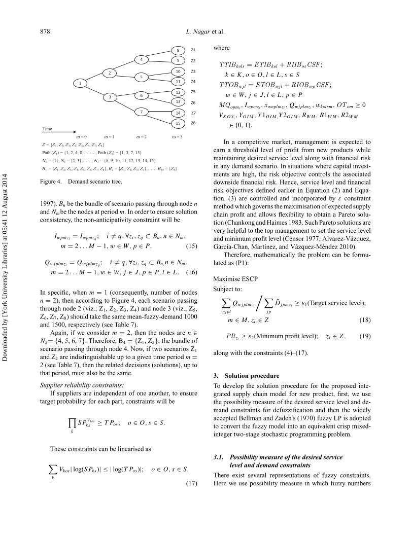
Figure 4. Demand scenario tree.
1997). Bn be the bundle of scenario passing through node nand Nmbe the nodes at period m. In order to ensure solutionconsistency, the non-anticipativity constraint will be
Iwpmzi= Iwpmzq
; i �= q,∀zi, zq ⊂ Bn, n ∈ Nm,
m = 2 . . . M − 1, w ∈ W,p ∈ P, (15)
Qwjplmzi= Qwjplmzq
; i �= q,∀zi, zq ⊂ Bn,n ∈ Nm,
m = 2 . . . M − 1, w ∈ W, j ∈ J, p ∈ P, l ∈ L. (16)
In specific, when m = 1 (consequently, number of nodesn = 2), then according to Figure 4, each scenario passingthrough node 2 (viz.; Z1, Z2, Z3, Z4) and node 3 (viz.; Z5,Z6, Z7, Z8) should take the same mean-fuzzy-demand 1000and 1500, respectively (see Table 7).
Again, if we consider m = 2, then the nodes are n ∈N2= {4, 5, 6, 7}. Therefore, B4 = {Z1, Z2}; the bundle ofscenario passing through node 4. Now, if two scenarios Z1
and Z2 are indistinguishable up to a given time period m =2 (see Table 7), then the related decisions (solutions), up tothat period, must also be the same.
Supplier reliability constraints:If suppliers are independent of one another, to ensure
target probability for each part, constraints will be
∏k
SPVkos
ks ≥ T Pos ; o ∈ O, s ∈ S.
These constraints can be linearised as
∑k
Vkos | log(SPks)| ≤ | log(T Pos)|; o ∈ O, s ∈ S,
(17)
where
TTIB kols = ETIB kol + RIIBosCSF ;
k ∈ K, o ∈ O, l ∈ L, s ∈ S
TTOBwjl = ETOBwjl + RIOBwpCSF ;
w ∈ W, j ∈ J, l ∈ L,p ∈ P
MQopmi, Iwpmzi
, xowplmzi,Qwjplmzi
, wkolsm,OT om ≥ 0
VKOS,, YOIM, Y1OIM,Y2OIM,RWM,R1WM,R2WM
∈ {0, 1}.
In a competitive market, management is expected toearn a threshold level of profit from new products whilemaintaining desired service level along with financial riskin any demand scenario. In situations where capital invest-ments are high, the risk objective controls the associateddownside financial risk. Hence, service level and financialrisk objectives defined earlier in Equation (2) and Equa-tion. (3) are controlled and incorporated by ε constraintmethod which governs the maximisation of expected supplychain profit and allows flexibility to obtain a Pareto solu-tion (Chankong and Haimes 1983. Such Pareto solutions arevery helpful to the top management to set the service leveland minimum profit level (Censor 1977; Alvarez-Vazquez,Garcıa-Chan, Martınez, and Vazquez-Mendez 2010).
Therefore, mathematically the problem can be formu-lated as (P1):
Maximise ESCP
Subject to:∑wjpl
Qwjplmzi
/ ∑jp
Djpmzi≥ ε1(Target service level);
m ∈ M, zi ∈ Z (18)
PRzi≥ ε2(Minimum profit level); zi ∈ Z, (19)
along with the constraints (4)–(17).
3. Solution procedure
To develop the solution procedure for the proposed inte-grated supply chain model for new product, first, we usethe possibility measure of the desired service level and de-mand constraints for defuzzification and then the widelyaccepted Bellman and Zadeh’s (1970) fuzzy LP is adoptedto convert the fuzzy model into an equivalent crisp mixed-integer two-stage stochastic programming problem.
3.1. Possibility measure of the desired servicelevel and demand constraints
There exist several representations of fuzzy constraints.Here we use possibility measure in which fuzzy numbers
Dow
nloa
ded
by [
Yor
k U
nive
rsity
Lib
rari
es]
at 0
5:41
12
Aug
ust 2
014
International Journal of Systems Science 879
are interpreted by the degree of uncertainty. Possibility (op-timistic sense) means the maximum chance (at least) tobe selected by the DM. Analogous to chance constrainedprogramming with stochastic parameters, in a fuzzy envi-ronment; it is assumed that some constraints may be satis-fied with a least possibility, η(0 ≤ η ≤ 1) (i.e. the ‘chance’is represented by the ‘possibility’). According to Duboisand Prade (1983), if A and B are two fuzzy numberswith membership functions μA(x) and μB(x), respectively,then
Pos(A∗B) = {sup(min(μA(x), μB(y)), x, y ∈ , x∗y},
where the abbreviation Pos (·) denotes the possibility of theevent in {·} and ∗ is any of the relations <,>,=,≤,≥.To be specific, the possibility measure of a fuzzy eventA ≥∈ can be defined as Pos(A ≥∈) = supx≥∈ μA(x), whereA = (Ap,Am,Ao) and ∈ is a real number (Liu and Iwamura1998; Li, Xu, and Gen 2006; Xu, Yao, and Zhao 2011).Consequently, the possibility measure of A ≥∈ can berepresented as
Pos(A ≥∈) =
⎧⎪⎪⎨⎪⎪⎩1, Am ≥∈,
Ao− ∈Ao − Am
, Am ≤∈≤ Ao,
0, Ao ≤∈ .
In other words, when ∈ is a crisp number, Pos(A≥∈) ≥ η if and only if Ao−∈
Ao−Am ≥ η.
Imprecise service level constraints:When the demand of the scenario are specified by triangularfuzzy number Djpmzi
(see Figure 2), the imprecise servicelevel constraints (18) are realised under the possibility mea-sure as
Pos
⎛⎝∑wjpl
Qwjplmzi
/ ∑jp
Djpmzi>∈1
⎞⎠ > η;
m ∈ M, zi ∈ Z
This means that the constraint is feasible if and only if itspossibility is at least η. Therefore, an equivalent determin-istic representations of the above constraint is∑
wjpl Qwjplmzi− ε1
∑jp D
pjpmzi
ε1( ∑
jp
(Dm
jpmzi− D
pjpmzi
)) > η;
or∑wjpl
Qwjplmzi≥ ε1
∑jp
Dpjpmzi
+ ε1η∑jp
(Dm
jpmzi− D
pjpmzi
);
m ∈ M, zi ∈ Z. (20)
Demand constraints:The imprecise demand constraint (14) can be written underthe possibility measure as
Pos
(∑wl
Qwjplmzi≤ Djpmzi
)> η;
j ∈ J, p ∈ P,m ∈ M, zi ∈ Z
or equivalently,
Dojpmzi
− ∑wl Qwjplmzi
Dojpmzi
− Dmjpmzi
> η;
or ∑wl
Qwjplmzi< Do
jpmzi− (
Dojpmzi
− Dmjpmzi
)η;
j ∈ J, p ∈ P,m ∈ M, zi ∈ Z. (21)
3.2. Fuzzy linear programming approach
The solution procedure using the fuzzy LP approach(Tanaka and Asai 1984) for the proposed integrated sup-ply chain model for new products has following steps:
Step 1: Construct the linear membership function ofESCP:
This is done by calculating the extreme lower and upperbounds of the ESCP values. The following sequence ofevents is included in this step:
• Identify four extreme optimisation problems us-ing different combination of production rates(Rop and Rop + F Rop) and supplier capacities(PAksm and PAksm + PDksm).
• Solve the multi-objective LP problem by consideringone objective at a time with related supply chainconstraints.
• Identify the extreme upper and lower bounds of ESCP.
Therefore, if ESCPl and ESCPu be the extreme lowerand upper bounds of ESCP, then the resultant membershipfunction μOFESCP (ESCP) for optimal values can be definedas
μOFESCP (ESCP)
=
⎧⎪⎪⎨⎪⎪⎩0,
(ESCP − ESCPl)/(ESCPu − ESCPl),
1,
ESCP < ESCPl
ESCPl ≤ ESCP ≤ ESCPu
ESCP ≥ ESCPu
(22)
In this formulation, if the supply chain profit is less thanlower bound, DM is totally unsatisfied and he/she will be
Dow
nloa
ded
by [
Yor
k U
nive
rsity
Lib
rari
es]
at 0
5:41
12
Aug
ust 2
014
880 L. Nagar et al.
totally satisfied when the supply chain profit reaches theupper bound. The degree of satisfaction increases with therise of supply chain profit between these two bounds.
Step 2: Construct the linear membership function forproduction time and supplier capacity constraints
Similar to the formulation of Equation (22),one can construct the linear membership functions,μcom
(∑
p RopMQopm) for fuzzy production rate and themembership function μckosm
(PAksmVkos) for fuzzy suppliercapacity.
These two membership functions can be interpreted asfollows:
For μcomof production time constraints, if the total time
required is more than available time then DM’s satisfactionis zero and DM is fully satisfied when the available time ismore at production tolerance point Rop + FRop.
For μckosmof supplier capacity constraints are subjective
valuation of the necessary quantity∑
kolsm Wkolsm with ref-erence to the available quantity PAksm . For example, if theparts requirement is less than supplier capacity than DM ishighly satisfied and, satisfaction level decreases when partsrequirement exceeds the upper limit of supplier capacity.
Step 3: Find a solution satisfying the objective goal andthe constraints:
To find a compromise point (λ) which satisfies the con-straints and the objective goal to the maximum extend, weuse Bellman and Zadeh’s (1970) approach. This is com-puted as follows:
λ = min
(μOFESCP (ESCP),
mino∈O,m∈M
(μcom
( ∑p
RopMQopm
)),
mink∈K, o∈O, s∈S, m∈M
(μckosm(PAksmVkos))
).
Considering the resultant membership values for theobjective and all the constraints, one need to maximise thedegree of satisfaction for the worst situation, i.e. maximiseλ. Consequently the problem becomes a deterministic op-timisation problem (P2) as shown below.
Max λ
s.t.λ(ESCPu − ESCPl) − ESCP + ESCPl ≤ 0∑
p
(Rop + λFRop)MQopm ≤∑
i
(Aoim + AOT oim)Yoim∑ol
Wkolsm ≤ PAksmVkos + (1 − λ)PDksmVkos
0 ≤ λ ≤ 1,
along with the constraints (4)–(7), (9), (11)–(13), (15)–(17),(20) and (21).
It should be noted that, mathematically, the relationshipbetween the optimal solutions of (P1) and (P2) can be statedas ‘If (x1, x2, . . . xn, λ) is an optimal solution of (P2), then(x1, x2, . . . xn) is an optimal solution of (P1)’. The con-straints in the problem (P2) contain the cross product termsλPDksm and λFRop that make the problem non-linear. Ifthe value of λis fixed, it can be reduced to a LP problem.
Step 4: Solve the reduced LP using two-stage stochasticprogramming approach:
Here we solve the reduced mixed integer LP with aspecific value of λ. In light of two-stage programming ap-proach, variables of this model are partitioned into twocategories based on whether the corresponding task needsto be carried out before or after demand realisation.
The sequence of events in this step is the following:
• Run the LP to decide first-stage design variables. Thevariables such as plant location, processing line perlocation, raw material procurement, capacity utilisa-tion and production, due to the significant lead timesassociated with these tasks, are determined as designdecisions, which need to be decided prior to demandrealisation.
• Set the parameter based on first-stage output. Thenthe system will be subjected to the random processdue to the presence of stochastic demand.
• Run the LP to obtain the second-stage solution. Inthis stage, the solution procedure will execute thepost-production activities such as inventory, shortageand supply of finished product to customer are deter-mined as control variables, which can be fine-tunedafter realisation of the actual demand.
Step 5: Execute and modify the interactive decisionprocess:
Obtaining the optimal solution λ∗of (P2) is equivalentto determining the maximum value of λ so that there existsan admissible set satisfying the constraints of (P2). Conse-quently, for each λ, test whether a feasible set of the problemexists or not and determine the maximum value of λ satisfy-ing the supply chain constraints until a satisfactory solutionis obtained.
4. The computational experience
To illustrate the effectiveness of the proposed integratedsupply chain model, we consider a simple supply chain net-work with single new product (consumer electronics prod-uct). This network has two potential plant locations (O1,O2) each of which can have two production lines (I1, I2),two potential warehouse locations (W1, W2), two suppli-ers (K1, K2), single raw material and two customer groups(J1, J2). For each production line three cost componentsare considered: one time installation cost, operating cost
Dow
nloa
ded
by [
Yor
k U
nive
rsity
Lib
rari
es]
at 0
5:41
12
Aug
ust 2
014
International Journal of Systems Science 881
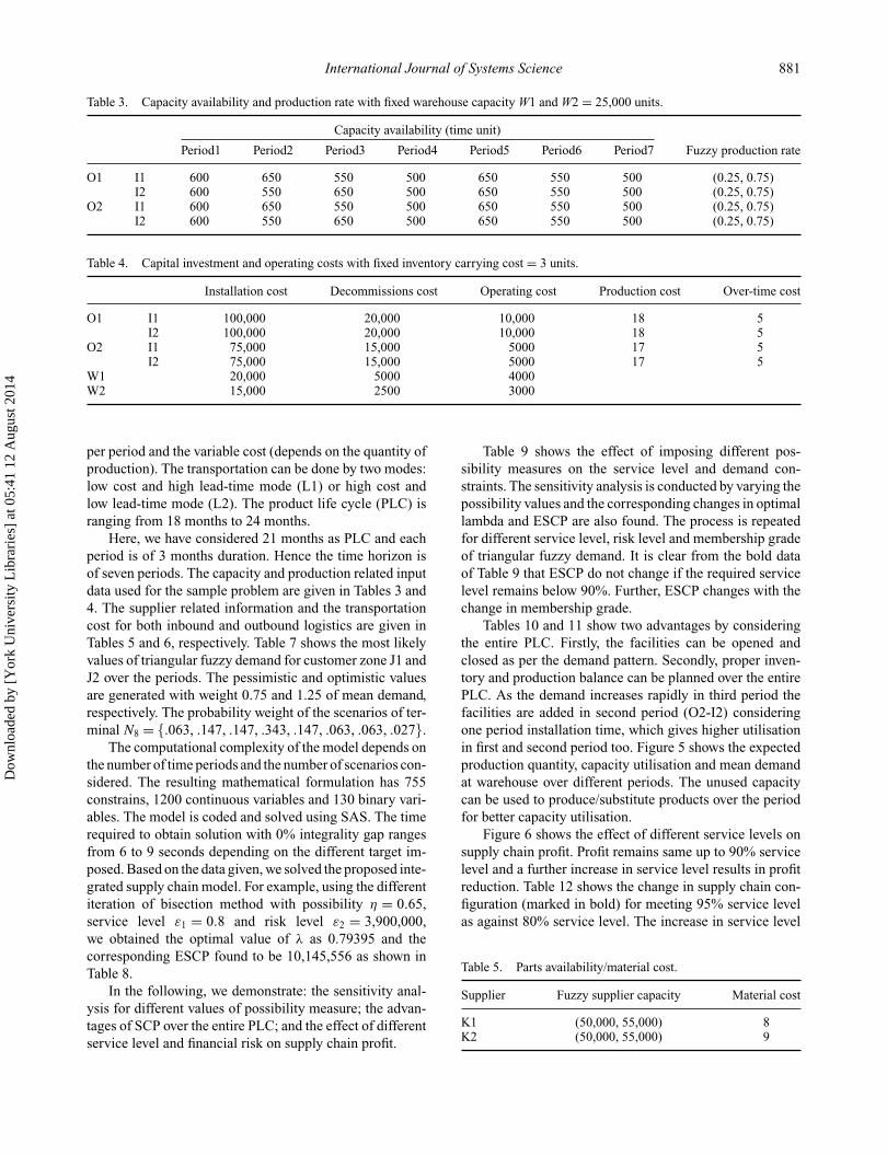
Table 3. Capacity availability and production rate with fixed warehouse capacity W1 and W2 = 25,000 units.
Capacity availability (time unit)
Period1 Period2 Period3 Period4 Period5 Period6 Period7 Fuzzy production rate
per period and the variable cost (depends on the quantity ofproduction). The transportation can be done by two modes:low cost and high lead-time mode (L1) or high cost andlow lead-time mode (L2). The product life cycle (PLC) isranging from 18 months to 24 months.
Here, we have considered 21 months as PLC and eachperiod is of 3 months duration. Hence the time horizon isof seven periods. The capacity and production related inputdata used for the sample problem are given in Tables 3 and4. The supplier related information and the transportationcost for both inbound and outbound logistics are given inTables 5 and 6, respectively. Table 7 shows the most likelyvalues of triangular fuzzy demand for customer zone J1 andJ2 over the periods. The pessimistic and optimistic valuesare generated with weight 0.75 and 1.25 of mean demand,respectively. The probability weight of the scenarios of ter-minal N8 = {.063, .147, .147, .343, .147, .063, .063, .027}.
The computational complexity of the model depends onthe number of time periods and the number of scenarios con-sidered. The resulting mathematical formulation has 755constrains, 1200 continuous variables and 130 binary vari-ables. The model is coded and solved using SAS. The timerequired to obtain solution with 0% integrality gap rangesfrom 6 to 9 seconds depending on the different target im-posed. Based on the data given, we solved the proposed inte-grated supply chain model. For example, using the differentiteration of bisection method with possibility η = 0.65,service level ε1 = 0.8 and risk level ε2 = 3,900,000,we obtained the optimal value of λ as 0.79395 and thecorresponding ESCP found to be 10,145,556 as shown inTable 8.
In the following, we demonstrate: the sensitivity anal-ysis for different values of possibility measure; the advan-tages of SCP over the entire PLC; and the effect of differentservice level and financial risk on supply chain profit.
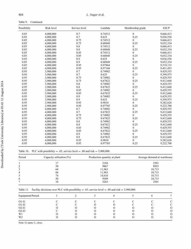
Table 9 shows the effect of imposing different pos-sibility measures on the service level and demand con-straints. The sensitivity analysis is conducted by varying thepossibility values and the corresponding changes in optimallambda and ESCP are also found. The process is repeatedfor different service level, risk level and membership gradeof triangular fuzzy demand. It is clear from the bold dataof Table 9 that ESCP do not change if the required servicelevel remains below 90%. Further, ESCP changes with thechange in membership grade.
Tables 10 and 11 show two advantages by consideringthe entire PLC. Firstly, the facilities can be opened andclosed as per the demand pattern. Secondly, proper inven-tory and production balance can be planned over the entirePLC. As the demand increases rapidly in third period thefacilities are added in second period (O2-I2) consideringone period installation time, which gives higher utilisationin first and second period too. Figure 5 shows the expectedproduction quantity, capacity utilisation and mean demandat warehouse over different periods. The unused capacitycan be used to produce/substitute products over the periodfor better capacity utilisation.
Figure 6 shows the effect of different service levels onsupply chain profit. Profit remains same up to 90% servicelevel and a further increase in service level results in profitreduction. Table 12 shows the change in supply chain con-figuration (marked in bold) for meeting 95% service levelas against 80% service level. The increase in service level
Table 5. Parts availability/material cost.
Supplier Fuzzy supplier capacity Material cost
K1 (50,000, 55,000) 8K2 (50,000, 55,000) 9
Dow
nloa
ded
by [
Yor
k U
nive
rsity
Lib
rari
es]
at 0
5:41
12
Aug
ust 2
014
882 L. Nagar et al.
Table 6. Transportation cost between inbound and outbound logistics.
Supplier and plants Plants and warehouses Warehouses and customer group
forces the installation of an additional production facility.This also demonstrates the significance of service level insupply chain design.
The risk objectives defined here control the situationswhere the profit cannot recede below a threshold (ε2). Insituations involving large amounts of capital investments,the associated downside financial risk must be controlled.In Table 13, the supply chain profit over different scenariosis listed for both without risk constraint and with risk con-straint. Assuming scenario 1 as base and minimum profitlevel at 6,000,000, the variability in profit is also obtained.It is shown that the weighted profit is less in case of riskconstraint but variation in profit is reduced by 3% and theprofit remains above a certain specified level.
4.1. Practical implications of the research
The intent of this research was to develop an integrateddecision model considering SCP uncertainties associatedwith new product. The supply chain design decision overthe life cycle of the product (opening/closing of facil-ities over the product life cycle) and SCP decisions inan integrated manner in a multi-objective decision envi-ronment (maximisation of profit, achieving desired ser-vice level and minimising risk) are addressed through thisresearch.
The integrated supply chain model will be highlyuseful to fashion apparel industry, high technologyconsumer electronic (mobile phones, tablets like i-pad,computer hardware, television) industry which introduces
Dow
nloa
ded
by [
Yor
k U
nive
rsity
Lib
rari
es]
at 0
5:41
12
Aug
ust 2
014
International Journal of Systems Science 883
Table 9. ESCP with different possibility, service level, risk level and membership grade.
Possibility Risk level Service level Lambda Membership grade ESCP
Table 11. Facility decisions over PLC with possibility = .65, service level = .80 and risk = 3,900,000.
Equipment/Period 1 2 3 4 5 6 7
O1-I1 C C C C C C CO1-I2 C C O O C C CO2-I1 O O O O O O OO2-I2 C O O O O O OW1 O O O O O O OW2 O O O O O O O
Note: O, open; C, close.
Dow
nloa
ded
by [
Yor
k U
nive
rsity
Lib
rari
es]
at 0
5:41
12
Aug
ust 2
014
International Journal of Systems Science 885
Figure 5. Optimal production planning.
Figure 6. Effect of service level on supply chain profit.
innovative products at rapid pace in a highly competitivemarket. The demand for these products is highly uncer-tain and unpredictable due to absence of past demanddata.
In Indian market, life cycles of these products arereducing ranging between 18 months to 24 months. Forexample, in fashion apparel industry, new and innovativedesign apparels are introduced in every season. Threecrucial factors in fashion consumption: market timing, costand the buying cycle. Timing’s objective is to create theshortest production time possible. Shortened buying cycledue to quick response manufacturing increased inventoryturnover and shortened forecast period. In such scenario,most of the input parameters such as demand, supplyas well as production processing time, distribution leadtime are uncertain and the developed model will help indesign and planning the supply chain that maximises theprofits.
Table 12. Facility decisions over PLC with possibility = .65, service level = .95 and risk = 3,900,000.
Equipment/Period 1 2 3 4 5 6 7
O1-I1 C C C C C C CO1-I2 C C C O O O OO2-I1 O O O O O O CO2-I2 C O O O O O CW1 O O O O O O OW2 O O O O O O O
Note: O, open; C: close.
Table 13. Profit over scenarios.
Scenario/Profit Without risk constraint % of variation With risk constraint % of variation
In this paper, we have proposed an integrated two-stagesupply chain model for new products considering impreciseproduction rate and supplier capacity under fuzzy randomdemand scenarios. The unique approach of considering sce-nario dependent fuzzy random demand for a multi-echelonnew product supply chain gives the advantage of coveringdemand uncertainty using scenario probabilities as well asimprecise information. The solution approach chosen al-lows simultaneous determination of optimum supply chaindesign, procurement and production quantities across dif-ferent plants and trade-offs between inventory and trans-portation modes (for both inbound and outbound logis-tics). The model and solution approach provides flexibilityto obtain a Pareto solution in a multi-objective decisionenvironment.
Our findings have suggested that it is advantageous todevelop supply chain plans over the entire PLC. Effec-tive capacity utilisation, appropriate mode of transporta-tion, proper supplier selection and the trade-off betweencapacity and inventory levels can be achieved by planningover the PLC. From sensitivity analysis, we have found thatexpected supply chain profit decreases with high values ofpossibility measure. The trade-off analysis presented in thepaper provides managerial insight to the DM to choose theappropriate supply chain configuration for desired servicelevel and financial risk keeping the expected supply chainprofit as per the policy of the organisation.
AcknowledgementsThe authors are grateful to the Associate Editor and the anonymousreferees for their valuable comments and suggestions.
Notes on contributorsLokesh Nagar is working as SoftwareManager at SAS R & D India Pvt Ltd. Hereceived his PhD degree from IIT Bombayin 2009. Before joining SAS, he has workedas a Research Scholar at IIT Bombay. Hismain areas of research interest includesupply chain modelling, multi-objectivedecision-making, data mining, forecastingand stochastic optimisation. Dr Nagar has
many publications in various international journals, patent, bookchapters and conferences.
Pankaj Dutta is an Assistant Professor ofShailesh J. Mehta School of Managementat IIT Bombay. He received his PhD degreefrom IIT Kharagpur in 2007. Before joiningSJMSOM, he has served as a Lecturerat BITS, Pilani. He has also worked asVisiting Research Fellow at EPFL, SwissFederal Institute of Technology, Lausanne.His main areas of research interest include
supply chain modelling, inventory management, reverse logistics,fuzzy optimisation and multi-objective decision-making. In 2005,while working on his PhD dissertation, he pioneered the concept
of fuzzy random demand in the field of inventory systems. DrDutta has many publications in various international journals,book chapters and conferences. He is also a reviewer of manyreputed international journals.
Karuna Jain (PhD, IIT Kharagpur; PostDoctoral Fellow, Faculty of Management,University of Calgary, Canada) is theMHRD IPR Chair Professor, at the ShaileshJ. Mehta School of Management, Indian In-stitute of Technology Bombay, India. Prof.Jain has extensive industrial and teachingexperience in the field of Operations andTechnology Management. Her active re-
search interests span across Strategic Management of Technologyand Innovation, Intellectual Property Strategy and Management,Project Management and Supply Chain Management. She hasbeen actively publishing her research in national and internationaljournals and conferences across the areas of Technology andOperations management (IAMOT, POMS, PICMET, WCIC andIFTM). Her joint research published in the Journal of IntellectualCapital won the - ‘Emerald Literati Network 2007 Awards forExcellence’ and has received best research paper awards ininternational conferences. Prof. Jain is the recipient of the “BestTeacher in Operations Management” in the 16th Business SchoolAffaire & Dewang Mehta Business School Awards, 2009 and“Best Professor in Operations Management in Asia” by CMOAsia, 2010. Prof. Jain serves on numerous academic, professionaland government bodies in various capacities like Member,Sectoral Innovation Council on Intellectual Property Rights underthe Department of Industrial Policy and Promotion, Ministry ofCommerce and Industry, Government of India, 2011–2012, Mem-ber, Decision Sciences Institute Board, 2011–2012, Regional VicePresident for the Decision Sciences Institute Indian SubcontinentRegion, 2011–2012, Vice Chairperson for Project ManagementInstitute - India Academic Advisory, from December 2011–12.
ReferencesAliev, R.A., Fazlollahi, B., Guirimov, B.G., and Aliev, R.R.
(2007), ‘Fuzzy-Genetic Approach to Aggregate Production-Distribution Planning in Supply Chain Management’, Infor-mation Sciences, 177, 4241–4255.
Alvarez-Vazquez, L.J., Garcıa-Chan, N., Martınez, A., andVazquez-Mendez, M.E. (2010), ‘Multi-Objective Pareto-Optimal Control: An Application to Wastewater Manage-ment’, Computational Optimization and Applications, 46,135–157.
Bellman, R.E., and Zadeh, L.A. (1970), ‘Decision-Making in aFuzzy Environment’, Management Science, 17, 141–164.
Butler, R.J., Ammons, J.C., and Sokol. J. (2003), ‘A Ro-bust Optimization Model for Strategic Production andDistribution Planning for a New Product’. Available athttp://citeseerx.ist.psu.edu.
Censor, Y. (1977), ‘Pareto Optimality in Multiobjective Prob-lems’, Applied Mathematics and Optimization, 4, 41–59.
Chankong, V., and Haimes, Y. (1983), Multiobjective Deci-sion Making Theory and Methodology, New York: ElsevierScience.
Chen, C.L., and Lee, W.C. (2004), ‘Multi Objective Optimizationof Multi Echelon Supply Chain Networks With UncertainProduct Demands and Prices’, Computers and Chemical En-gineering, 28, 1131–1144.
Dow
nloa
ded
by [
Yor
k U
nive
rsity
Lib
rari
es]
at 0
5:41
12
Aug
ust 2
014
International Journal of Systems Science 887
Chen, C.T., Lin C.T., and Huang, S.F. (2006), ‘A Fuzzy Ap-proach for Supplier Valuation and Selection in Supply ChainManagement’, International Journal of Production Eco-nomics, 102, 289–301.
Dutta, P., Chakraborty, D., and Roy, A.R. (2005), ‘A Sin-gle Period Inventory Model With Fuzzy Random VariableDemand’, Mathematical and Computer Modeling, 41, 915–922.
Dutta, P., Chakraborty, D., and Roy, A.R. (2007), ‘Continuous Re-view Inventory Model in Mixed Fuzzy and Stochastic Envi-ronment’, Applied Mathematics and Computation, 188, 970–980.
Dogan, K., and Goetschalckx, M. (1999), ‘A Primal De-composition Method for the Integrated Design of Multi-Period Production-Distribution Systems’, IIE Transactions,31, 1027–1036.
Dubois, D., and Prade, H. (1983), ‘Ranking Fuzzy Numbers inthe Setting of Possibility Theory’, Information Sciences, 30,183–224.
Escudero, L.F., Galindo, E., Garcia, G., Gomez, E., and Sabau,V. (1999), ‘Schumann, a Modeling Framework for SupplyChain Management Under Uncertainty’, European Journalof Operational Research, 119, 14–34.
Gaonakar, R., and Viswanadham, N. (2003), ‘Supply ChainPlanning Over Product Lifecycles’, in Proceedings of 2003IEEE/RSJ, Las Vegas, Nevada, pp. 2329–2334.
Gupta, A., and Maranas, C.D. (2003), ‘Managing Demand Uncer-tainty In Supply Chain Planning’, Computers and ChemicalEngineering, 27, 1219–1227.
Hu, J.S., Zheng, H., Xu, R.Q., Ji, Y.P., and Guo, C.Y. (2010), ‘Sup-ply Chain Coordination for Fuzzy Random Newsboy ProblemWith Imperfect Quality’, International Journal of Approxi-mate Reasoning, 51, 771–784.
Ishii, K., Takahashi, K., and Muramatsu, R. (1988), ‘Inte-grated Production, Inventory and Distribution Systems’,International Journal of Production Research, 26, 473–482.
Li, J., Xu, J., and Gen, M. (2006), ‘A Class of Multi-ObjectiveLinear Programming Model With Fuzzy Random Coeffi-cients’, Mathematical and Computer Modelling, 44, 1097–1113.
Liang, T.F. (2008), ‘Fuzzy Multi-Objective Produc-tion/Distribution Planning Decisions with Multi-Productand Multi-Time Period in a Supply Chain’, Computers andIndustrial Engineering, 55, 676–694.
Liu, B., and Iwamura, K.B. (1998), ‘Chance Constraint Program-ming With Fuzzy Parameters’, Fuzzy Sets and Systems, 94,227–237.
Messina, E., and Mitra, G. (1997), ‘Modeling and Analysis ofMultistage Stochastic Programming Problems: A SoftwareEnvironment’, European Journal of Operational Research,101, 343–359.
Min, H., and Zhou, G. (2002), ‘Supply Chain Modeling: Past,Present and Future’, Computers and Industrial Engineering,43, 231–249.
Nagar, L., and Jain, K. (2008), ‘Supply Chain Planning UsingMulti-stage Stochastic Programming. Supply Chain Manage-ment’, An International Journal, 13, 251–256.
Peidro, D., Mula, J., Poler, R., and Verdegay, J.L. (2009), ‘FuzzyOptimization for Supply Chain Planning Under Supply,Demand and Process Uncertainties’, Fuzzy Sets and Systems,160, 2640–2657.
Petrovic, D., Roy, R., and Petrovic, R. (1999), ‘Supply Chain Mod-elling Using Fuzzy Sets’, International Journal of ProductionEconomics, 59, 443–453.
Petrovic, D., Xie, Y., Burnham, K., and Petrovic, R. (2008), ‘Coor-dinated Control of Distribution Supply Chains in the Presenceof Fuzzy Customer Demand’, European Journal of Opera-tional Research, 185, 146–158.
Puri, M.L., and Ralescu, D.A. (1986), ‘Fuzzy Random Vari-ables’, Journal of Mathematical Analysis and Applications,114, 409–422.
Santoso, T., Ahmed, S., Goetschalckx, M., and Shapiro, A. (2005),‘A Stochastic Programming Approach for Supply Chain Net-work Design Under Uncertainty’. European Journal of Oper-ational Research, 167, 96–115.
Tanaka, H., and Asai, K. (1984), ‘Fuzzy Linear ProgrammingProblems With Fuzzy Numbers’, Fuzzy Sets and Systems, 13,1–10.
Torabi, S.A., and Hassini, E. (2008), ‘An Interactive PossibilisticProgramming Approach for Multiple Objective Supply ChainMaster Planning’, Fuzzy Sets and Systems, 159, 193–214.
Wang, J., and Shu, Y.F. (2005), ‘Fuzzy Decision Modeling forSupply Chain Management’, Fuzzy Sets and Systems, 150,107–127.
Xie, Y., Petrovic, D., and Burnham, K. (2006), ‘A Heuristic Pro-cedure for the Two-Level Control of Serial Supply ChainsUnder Fuzzy Customer Demand’, International Journal ofProduction Economics, 102, 37–50.
Xu, J., and Liu, Y. (2008), ‘Multi-Objective Decision MakingModel Under Fuzzy Random Environment and its Applica-tion to Inventory Problems’, Information Science, 178, 2899–2914.
Xu, J., Yao, L., and Zhao, X. (2011), ‘A Multi-Objective Chance-Constrained Network Optimal Model With Random FuzzyCoefficients and its Application to Logistics DistributionCenter Location Problem’, Fuzzy Optimization and DecisionMaking, 10, 255–285.
Xu, J., and Zhou, X. (2011), Fuzzy-like Multiple ObjectiveDecision Making, Studies in Fuzziness and Soft Computing(Vol. 263), Berlin/Heidelberg: Springer-Verlag.
Xu, R., and Zhai, X. (2008), ‘Optimal Models for Single-PeriodSupply Chain Problems With Fuzzy Demand’, InformationSciences, 178, 3374–3381.