An interface-enriched generalized ﬁnite element method for...

INTERNATIONAL JOURNAL FOR NUMERICAL METHODS IN ENGINEERINGInt. J. Numer. Meth. Engng 2010; 00:1–19Published online in Wiley InterScience (www.interscience.wiley.com). DOI: 10.1002/nme

An interface-enriched generalized finite element method forproblems with discontinuous gradient fields

Soheil Soghrati 1, Alejandro M. Aragon 1, C. Armando Duarte 1,Philippe H. Geubelle 2 3 ∗

1Department of Civil and Environmental Engineering, University of Illinois at Urbana-Champaign, 205 North

Mathews Avenue, Urbana, IL 61801, USA2

Beckman Institute of Advanced Science and Technology, University of Illinois at Urbana-Champaign, 405 North

Mathews Avenue, Urbana, IL 61801 USA3

Department of Aerospace Engineering, University of Illinois at Urbana-Champaign, 104 South Wright Street,

Urbana, IL 61801, USA

SUMMARY

A new Generalized Finite Element Method (GFEM) is introduced for solving problems with discontinuousgradient fields. The method relies on enrichment functions associated with generalized degrees of freedom atthe nodes generated from the intersection of the phase interface with element edges. The proposed approachhas several advantages over conventional GFEM formulations, such as a lower computational cost, easierimplementation, and straightforward handling of Dirichlet boundary conditions. A detailed convergencestudy of the proposed method and a comparison with the standard Finite Element Method (FEM) arepresented for heat transfer problems. The method achieves the optimal rate of convergence using meshesthat do not conform to the interfaces present in the domain while achieving a level of accuracy comparableto that of the standard FEM with conforming meshes. Various application problems are presented, includingthe conjugate heat transfer problem encountered in microvascular materials. Copyright c 2010 John Wiley& Sons, Ltd.

Received . . .

KEY WORDS: GFEM/XFEM; Heat transfer; Convection-diffusion equation; Gradient discontinuity;Enrichment functions; Microvascular materials

1. INTRODUCTION

Several problems in materials science and engineering include solution fields that areC0−continuous. Classical examples include thermal or structural fields in composite materialswhere the difference in material properties between the phases leads to discontinuities in thegradient field, also known as weak discontinuities [1, 2]. Another example can be found in themesoscale modeling of polycrystalline materials where the mismatch in material properties at grainsboundaries leads to a discontinuous gradient field [3]. In the general case, the mismatch betweenthe phases involves not only the difference between material properties, but also the effective termsin the governing differential equation based on the type of materials, e.g., conjugate fluid/solidproblems. Active cooling of materials through embedded microvascular networks [4] is an exampleof such problems, where, in addition to material properties, the effect of the convection in the fluidphase must be incorporated in the numerical solution.

∗Correspondence to: Philippe H. Geubelle, Beckman Institute of Advanced Science and Technology, University ofIllinois at Urbana-Champaign, 405 North Mathews Avenue, Urbana, IL 61801 USA. E-mail: [email protected]

Contract/grant sponsor: AFOSR MURI; contract/grant number: F49550-05-1-0346

Copyright c 2010 John Wiley & Sons, Ltd.Prepared using nmeauth.cls [Version: 2010/05/13 v3.00]

2 INTERFACE-ENRICHED GFEM FOR PROBLEMS WITH DISCONTINUOUS GRADIENT FIELDS

An accurate FEM solution for such problems can only be achieved by adopting a conformingmesh, i.e., a mesh that conforms to the interface geometry. In this case, the inherent gradientdiscontinuity between adjacent finite elements in the standard FEM accurately represents theweak discontinuity at the material interface. However, creating a conforming mesh which canappropriately represent the actual geometry of the structure while yielding elements with acceptableaspect ratios is a complex and often expensive process. Moreover, in some cases such as transientor optimization problems, where the geometry of the problem is changing throughout the analysis,the use of conforming meshes may simply be impossible [5, 6].

The aforementioned limitations of the standard FEM in handling problems with weak or strongdiscontinuities, where the latter refers to discontinuities in the solution field, have motivatedthe development of special numerical techniques. Among the most promising related methodsis the Generalized Finite Element Method (GFEM)/eXtended Finite Element Method (XFEM)[7, 8, 9, 10], which aims at providing independence between the problem morphology and thefinite element mesh used in the numerical solution. This is achieved by incorporating an a prioriknowledge of the solution field in the form of enrichment functions at the nodes of elements cutby the the interface. Thus, despite the inherent geometrical complexity for determining the locationof elements with respect to interface edges in 2D or surfaces in 3D, these methods provide a greatsimplification in modeling discontinuous phenomena with non-conforming meshes.

Early contributions to the GFEM/XFEM were directed towards linear-elastic fracture mechanicsand crack growth simulations [11, 12, 13, 14, 15]. Later contributions to the developement ofGFEM/XFEM for this type of problems can be found in [16, 17, 18, 19]. The implementationof these methods also gained interest in other areas addressing problems with weak and strongdiscontinuities. Such areas can be categorized but not limited to contact problems [14, 20],multiscale problems [21], multiphase/solidification [22, 23], and material or phase interfaces[24, 25, 26]. The current work focuses on the latter type of problems by introducing new enrichmentfunctions and a different approach for applying them at the interface. In the proposed method, thegeneralized degrees of freedom (dofs) are not applied to nodes of the original mesh, but consideredat the nodes that are created by intersecting the phase interface with element edges. Since thegeneralized dofs in this approach are applied to the interface nodes, we refer to the method asInterface Generalized Finite Element Method (IGFEM).

The remainder of the paper is organized as follows: In the next section, we discuss the formulationof the model problem that motivated this work, i.e., the convection-diffusion equation, and thecorresponding GFEM formulation. In Section 3, we introduce the enrichment functions used inthe IGFEM and explain its formulation for solving the model problem with three-node triangularelements. Also, implementation issues of the IGFEM are discussed and compared to those of moreconventional GFEM formulations for which generalized dofs are applied to the nodes of the originalmesh. It must be noted that the application of the IGFEM is not limited to the convection-diffusionequation and can be easily extended to other problems (such as structural problems) with weakdiscontinuities. A detailed convergence study for this method is provided in Section 4 by comparingthe accuracy and convergence rates with those of the standard FEM. We then apply the IGFEMto solve heat transfer problems in heterogeneous and actively-cooled microvascular materials inSection 5.

2. PROBLEM DESCRIPTION

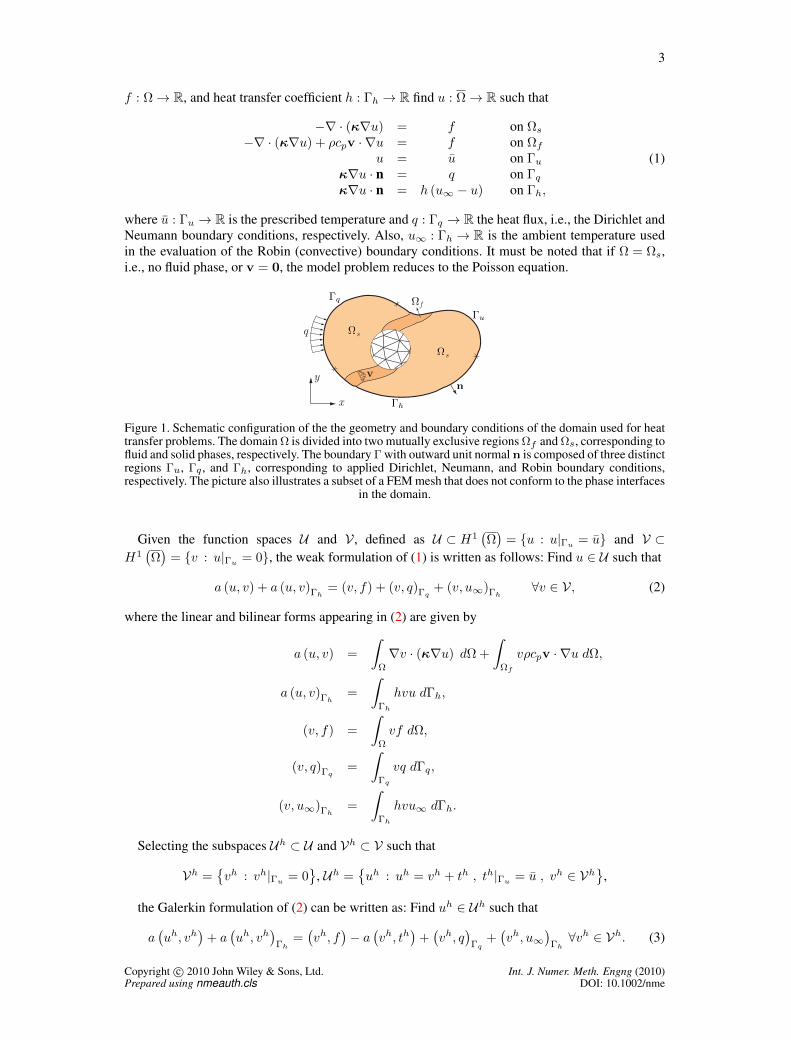
Consider an open domain Ω = Ωs ∪ Ωf ⊂ R2, Ωs ∩ Ωf = ∅, composed of two mutually exclusivesolid (Ωs) and fluid (Ωf ) regions, with closure Ω as shown in Figure 1. The boundary Γ = Ω− Ωhas an outward unit normal n and is divided into three distinct partitions Γu, Γq, and Γh such thatΓ = Γu ∪ Γq ∪ Γh and Γu ∩ Γq ∩ Γh = ∅. The strong form of the convection-diffusion boundaryvalue problem can then be expressed as follows: Given the thermal conductivity κ : Ω → R2 ×R2,fluid density ρ : Ωf → R, fluid specific heat cp : Ωf → R, velocity field v : Ωf → R2, heat source

Copyright c 2010 John Wiley & Sons, Ltd. Int. J. Numer. Meth. Engng (2010)Prepared using nmeauth.cls DOI: 10.1002/nme

3

f : Ω → R, and heat transfer coefficient h : Γh → R find u : Ω → R such that

−∇ · (κ∇u) = f on Ωs

−∇ · (κ∇u) + ρcpv ·∇u = f on Ωf

u = u on Γu

κ∇u · n = q on Γq

κ∇u · n = h (u∞ − u) on Γh,

(1)

where u : Γu → R is the prescribed temperature and q : Γq → R the heat flux, i.e., the Dirichlet andNeumann boundary conditions, respectively. Also, u∞ : Γh → R is the ambient temperature usedin the evaluation of the Robin (convective) boundary conditions. It must be noted that if Ω = Ωs,i.e., no fluid phase, or v = 0, the model problem reduces to the Poisson equation.

n

Γq

Γu

x

Ωs

Ωs

Ωf

v

q

Γh

y

Figure 1. Schematic configuration of the the geometry and boundary conditions of the domain used for heattransfer problems. The domain Ω is divided into two mutually exclusive regions Ωf and Ωs, corresponding tofluid and solid phases, respectively. The boundary Γ with outward unit normal n is composed of three distinctregions Γu, Γq , and Γh, corresponding to applied Dirichlet, Neumann, and Robin boundary conditions,respectively. The picture also illustrates a subset of a FEM mesh that does not conform to the phase interfaces

in the domain.

Given the function spaces U and V , defined as U ⊂ H1Ω= u : u|Γu = u and V ⊂

H1Ω= v : u|Γu = 0, the weak formulation of (1) is written as follows: Find u ∈ U such that

a (u, v) + a (u, v)Γh= (v, f) + (v, q)Γq

+ (v, u∞)Γh∀v ∈ V, (2)

where the linear and bilinear forms appearing in (2) are given by

a (u, v) =

Ω

∇v · (κ∇u) dΩ+

Ωf

vρcpv ·∇u dΩ,

a (u, v)Γh=

Γh

hvu dΓh,

(v, f) =

Ω

vf dΩ,

(v, q)Γq=

Γq

vq dΓq,

(v, u∞)Γh=

Γh

hvu∞ dΓh.

Selecting the subspaces Uh ⊂ U and Vh ⊂ V such that

Vh =vh : vh|Γu = 0

, Uh =

uh : uh = vh + th , th|Γu = u , vh ∈ Vh

,

the Galerkin formulation of (2) can be written as: Find uh ∈ Uh such that

auh, vh

+ a

uh, vh

Γh

=vh, f

− a

vh, th

+vh, q

Γq

+vh, u∞

Γh

∀vh ∈ Vh. (3)



Equation (3) can be directly used as the standard FEM approximation by discritizing the domain Ωinto m finite elements (Ω ∼= Ωh ≡ ∪m

i=1Ωi ) and employing a set of n standard Lagrangian shapefunctions Ni (x) for approximating the field in each element such that

uh (x) =n

i=1

Ni (x)ui. (4)

If a non-conforming mesh as shown in Figure 1 is adopted, the Galerkin method is not capableto capture the gradient discontinuity at the interfaces, which introduces a substantial error andtherefore a loss of the optimal rate of convergence. This problem can be addressed by enrichingthe solution space at the nodes of elements intersecting with the material interface to retrieve themissing information in the standard FEM solution. Within the GFEM framework, this can be doneby using a set of local enrichment functions ϕij (x) : x → R | Ni (x) = 0nen

j=1 where nen is thenumber of enrichment functions associated with node i. The approximation of the solution fieldthrough the GFEM is then expressed as

uh (x) =n

i=1

Ni (x) ui +n

i=1

Ni (x)nen

j=1

ϕij (x) uij . (5)

The first term of (5) is similar to the standard FEM approximation except for the fact that ui doesnot in general represent the field value at node i because of the presence of the second term in (5),which is associated with the contribution of enrichment functions in evaluating the nodal values ofthe solution. These enrichment functions are multiplied by the standard Lagrangian shape functionsto provide a sparse resulting system of linear equations. It is worth mentioning that, although (5)seems to indicate that all nodes are enriched, this does not have to be the case in general.

Several issues are raised by the implementation of the GFEM formulation described by (5). Thefirst issue involves handling the Dirichlet boundary conditions at the enriched nodes of the mesh.Based on (5), the field value at node i is given by ui = ui +

nen

j=1 ϕij (xi) uij . Since both ui anduij are unknown values, the prescribed value of the solution field can not be directly assigned tothe enriched node. Instead, one must employ techniques such as the penalty method or Lagrangemultipliers to enforce Dirichlet boundary conditions [27, 28]. One could shift ϕij such that it is zeroat the nodes. But, the enforcement of boundary conditions between the nodes is still problematic. Itis worth mentioning that for some enrichment functions such as those proposed in [26], the value ofthe enrichment function vanishes at the nodes and hence enforcing the Dirichlet boundary conditionsin the GFEM is as straightforward as in the standard FEM.

Another issue associated with the implementation of the GFEM involves in the blending ofrepresenting elements, i.e., elements with attached enrichment to all nodes, to conventional finiteelements. The problem arises due to the fact that only some of the nodes in the blending elementsare enriched and thus the enrichment functions are not fully reproduced through the interpolationwith Lagrangian shape functions described by (5). Hence, the incomplete terms of the enrichmentfunctions added to the numerical approximation in such elements may in fact deteriorate theaccuracy and rate of convergence. For linear interpolations, a solution is presented in [29] where allthe nodes of blending elements are enriched through the implementation of corrective enrichmentfunctions. However, as described in [25], higher order interpolations do not have the aforementionedproblem and optimal rates of convergences are recovered.

The last implementation issue that we study here is the quadrature of enriched elements in theGFEM. Because of the inherent weak discontinuities in these functions, using the same order ofGauss points as that used in the standard FEM in these elements leads to a considerable errorand degradation of the rate of convergence. It has also been shown that using higher-order Gaussquadratures in this case performs poorly in improving the accuracy [30]. Among several approachesproposed to address this problem, one of the most commonly accepted techniques consists insubdividing the element into subdomain elements and moving the standard quadrature from theparent element into these so called integration elements [12, 13]. The only constraint on creatingintegration elements is that their boundaries must be aligned with discontinuity edges or surfaces of


5

the domain and their aspect ratio does not affect the accuracy of the solution. As explained in thenext section, the IGFEM addresses some of the implementation issues associated with the GFEM.

3. IGFEM: FORMULATION AND IMPLEMENTATION

To explain the basic idea behind the IGFEM formulation, we first study two different approachesfor interpolating the solution field in a bi-material domain, as shown in Figure 2. The standard FEMinterpolation of the field when the domain is divided into two conforming elements is depictedin Figure 2(a). Assuming that the nodal values of the field ui are given and elements are locallynumbered counter-clockwise starting from the lower left node (Figure 2(b)), the interpolation of thefield using the Lagrangian shape functions in each element is given by

uh = N (1)1 u1 +N (1)

2 u2 +N (2)3 u3 +N (2)

4 u4 (6)

+N (1)

4 +N (2)1

u5 +

N (1)

3 +N (2)2

u6,

where N (j)i denotes the standard Lagrangian shape function associated with the i-th node of element

j.

Element 1

(a) (b) (c)

Element 2+= Parent element

34

21Element 1

Element 2

u1

u2

u3u4

u6

u

5u5

u

6

u5 − u

5

u6 − u

6

Figure 2. Two equivalent approaches for capturing the weak discontinuity at the phase interface (shown bya dash-dotted line) with Lagrangian shape functions: (a) standard FEM interpolation with two conformingelements, (b) interpolation with one non-conforming element, (c) missing part of the field interpolation with

the non-conforming element given in Figure (b).

On the other hand, if the two elements are merged to form one non-conforming element, the fieldapproximation with bilinear shape functions in the parent element, N (p)

i , looks like the one shownin Figure 2(b). In this case, the standard FEM interpolation is not able to reconstruct the gradientdiscontinuity at the material interface and hence the values u

5 and u

6 at the intersection of theelement edges with the interface are different from the given values u5 and u6. The missing partof the field in this interpolation can be retrieved as shown in Figure 2(c). An interpolation of thesolution field equivalent to that given in (6) is then obtained as

uh = N (p)1 u1 +N (p)

2 u2 +N (p)3 u3 +N (p)

4 u4 (7)

+N (1)

4 +N (2)1

u5 − u

5

+N (1)

3 +N (2)2

u6 − u

6

,

where N (p)i denoted the standard Lagrangian shape functions in the parent element. The above

equation can be rewritten as

uh = N (p)1 u1 +N (p)

2 u2 +N (p)3 u3 +N (p)

4 u4 + ψ1α1 + ψ2α2, (8)

where, similar to the GFEM formulation, ψ1 = N (1)4 +N (2)

1 and ψ2 = N (1)3 +N (2)

2 are consideredas enrichment functions and α1 and α2 are interpreted as generalized dofs. We can then extend (8)



into the formulation of the IGFEM as

uh (x) =n

i=1

Ni (x)ui +nen

i=1

sψi (x)αi, (9)

where the coefficient s is a scaling factor that will be introduced later.Several important characteristics of the IGFEM can be observed by comparing (9) with the

formulation of the conventional GFEM in (5). Similar to the conventional GFEM, the first termof (9) represents the standard FEM portion of the approximation. However, unlike the conventionalGFEM, the coefficients associated with the first term in the IGFEM directly correspond to the valuesof the field at each node. The second term in (9) denotes the effect of the enrichment functions inthe solution field because the enrichment functions vanish at these locations. The main differencebetween this term and the corresponding term in (5) is the approach for assembling the generalizeddegrees of freedom. While the partition of unity, i.e.,

ni=1 Ni (x) = 1, is used in the conventional

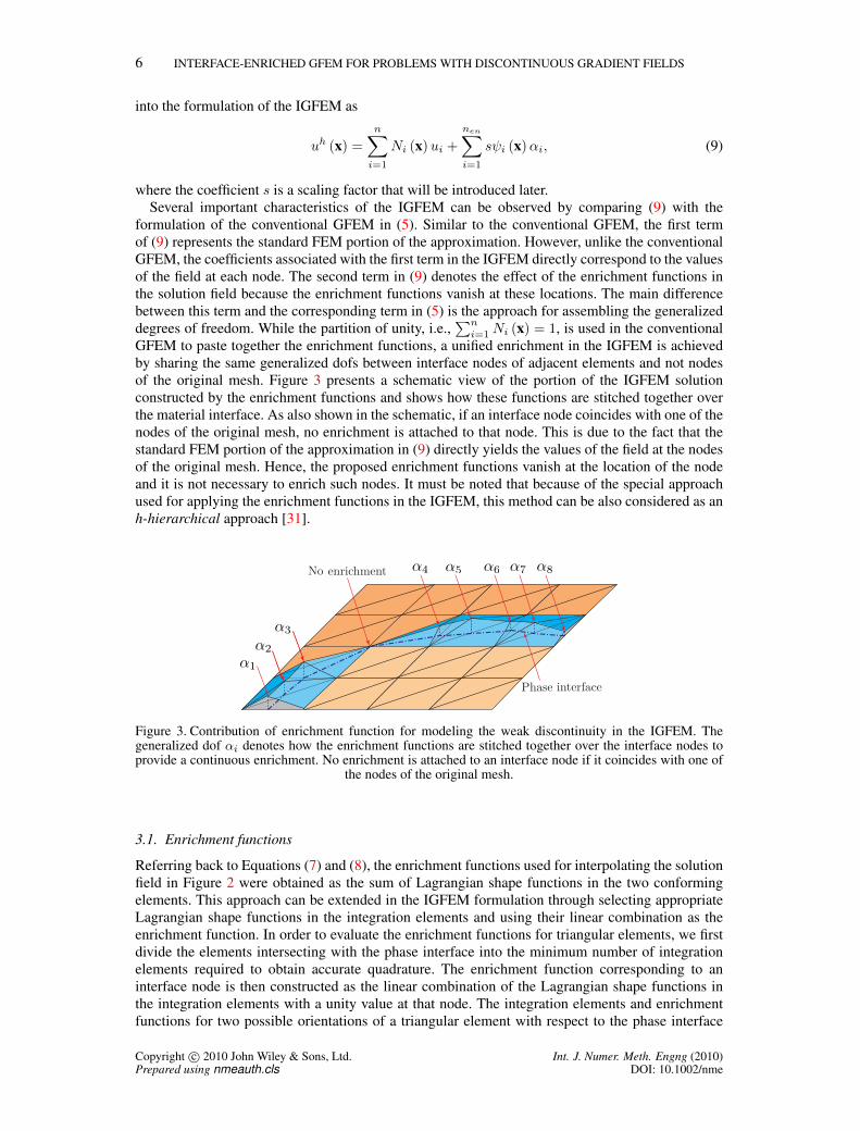
GFEM to paste together the enrichment functions, a unified enrichment in the IGFEM is achievedby sharing the same generalized dofs between interface nodes of adjacent elements and not nodesof the original mesh. Figure 3 presents a schematic view of the portion of the IGFEM solutionconstructed by the enrichment functions and shows how these functions are stitched together overthe material interface. As also shown in the schematic, if an interface node coincides with one of thenodes of the original mesh, no enrichment is attached to that node. This is due to the fact that thestandard FEM portion of the approximation in (9) directly yields the values of the field at the nodesof the original mesh. Hence, the proposed enrichment functions vanish at the location of the nodeand it is not necessary to enrich such nodes. It must be noted that because of the special approachused for applying the enrichment functions in the IGFEM, this method can be also considered as anh-hierarchical approach [31].

α1

α2

α3

α4 α5

Phase interface

No enrichment α6 α8α7

Figure 3. Contribution of enrichment function for modeling the weak discontinuity in the IGFEM. Thegeneralized dof αi denotes how the enrichment functions are stitched together over the interface nodes toprovide a continuous enrichment. No enrichment is attached to an interface node if it coincides with one of

the nodes of the original mesh.

3.1. Enrichment functions

Referring back to Equations (7) and (8), the enrichment functions used for interpolating the solutionfield in Figure 2 were obtained as the sum of Lagrangian shape functions in the two conformingelements. This approach can be extended in the IGFEM formulation through selecting appropriateLagrangian shape functions in the integration elements and using their linear combination as theenrichment function. In order to evaluate the enrichment functions for triangular elements, we firstdivide the elements intersecting with the phase interface into the minimum number of integrationelements required to obtain accurate quadrature. The enrichment function corresponding to aninterface node is then constructed as the linear combination of the Lagrangian shape functions inthe integration elements with a unity value at that node. The integration elements and enrichmentfunctions for two possible orientations of a triangular element with respect to the phase interface


7

are presented in Figure 4. As shown in this figure, the parent element is divided into either twotriangular elements or one triangular and one quadrilateral element based on the position of thephase interface. It must be noted that evaluating the enrichment functions in quadrilateral elementsis similar: first divide the element into two triangular sub-elements and then interact each triangularelement with the interface and enrich them as explained. These triangular subelements are onlygenerated for evaluated the enrichment functions and the shape functions used in the first term of(9) are still obtained from quadrilateral elements.

23

1

2

3

1

34

12

12

3

=⇒

=⇒ =⇒

Phase interf

ace

Phase interface2

1

1

(2)

(2)

(1)

(1)

=⇒ψ1

ψ2

ψ1 (x) = N (1)1 (x) +N (2)

1 (x)

ψ1 (x) = N (1)1 (x) +N (2)

2 (x)

ψ2 (x) = N (1)2 (x) +N (2)

1 (x)

Figure 4. Evaluation of the enrichment functions in the IGFEM: two scenarios for creating the integrationelements and corresponding enrichment functions based on the location of the interface in the intersected

triangular element.

As mentioned before, the aspect ratio of integration elements in the GFEM, and similarly in theIGFEM, does not affect the accuracy of the solution. However, since enrichment functions in theIGFEM are created from the Lagrangian shape functions associated to the integration elements,numerical difficulties arise if an interface node is too close to one of the nodes of the parentelement. In this case, the high aspect ratio of resulting integration elements and consequently thelarge gradient values of the corresponding enrichment functions may lead to the formation of an ill-conditioned stiffness matrix. In fact, this issue is a substantial problem in adaptive methods wherecreation of a conforming mesh from the original mesh is desired and often special techniques arerequired for handling the resulting ill-conditioned matrices [32].

To avoid the obove problem, we can scale the enrichment functions to control their gradient valuesin the numerical solution [26]. It must be remembered that the closer an interface node is locatedto one of the nodes of the parent element, the smaller the corresponding coefficient αi appearing in(9). Thus, one can scale down the enrichment functions as the interface node gets closer to one ofthe nodes of the parent element’s edge without affecting their performance in modeling the gradientdiscontinuity along the interface. In other words, instead of using the original enrichment functionsin this case, which leads to a very large gradient value and yields a vanishing coefficient αi, scalingdown the enrichment function controls the gradient value while avoiding an excessively large valueof αi. The relative location of the intersection point along the edge of the element is quantified by

:=min (x1 − xint , x2 − xint)

x2 − x1, (10)

where x1 and x2 are the nodes defining the intersecting edge of the parent element with the interface,and xint is the intersection point over this edge. We then scale the enrichment function by factors = 42, appearing in (9), which is a parabolic functions with a unity value in the middle of the



element’s edge and zero at its defining nodes (Figure 5), This scaling can be introduced for anyvalue of , or only when it is below a chosen threshold (say, < 0.01).

=⇒

Before scaling After scaling

1 1s

Figure 5. Scaling the enrichment functions using a parabolic function based on the distance between aninterface node and nodes of the element’s edge to avoid ill-conditioning. The dash-dotted line denotes the

location of the interface.

When a straight interface completely splits an element, the proposed IGFEM enrichmentfunctions resemble the ridge enrichments proposed in [26], which were based on the level setmethod. Instead, the IGFEM uses a linear combination of the Lagrangian shape functions in theintegration elements for constructing the enrichment functions. Also, in the IGFEM, the generalizedDOFs are attached to the interfaces nodes and we no longer employ the partition of unity forattaching enrichment to the nodes of the original mesh.

Furthermore, the IGFEM provides more flexibility for evaluating the enrichment functions inelements cut by piecewise linear interfaces or interfaces intersecting within an element. For instance,consider a three-node triangular element cut by an interface defined by two intersecting linearsegments as shown in Figure 6. Unlike the level set approach described in [26], the proposed IGFEMformulation is able to capture this type of interface geometry by dividing the parent element intothe minimum number of integration elements needed for accurate quadrature and using a linearcombination of the Lagrangian shape functions in these elements to obtain the enrichment functions.We only need to add an interface node at the intersection point of the interface segments and adda generalized dof there to capture the gradient jump at this location. The integration elements andcorresponding enrichment functions for the element cut by an interface with weak discontinuity arepresented in Figure 6. The same approach can be easily extended for evaluating the enrichmentfunctions in elements cut by three or more intersecting interfaces. Moreover, one can add oneor more interface nodes over the interface inside an element as shown in Figure 6 to reduce thegeometry approximations error associated with curved interfaces.

=⇒23

1

ψ1 ψ2

(2)

4

3

2 1

(3)3

4

2

1

(1)

3

2

1

ψ3

ψ1 = N (1)1 +N (2)

3

N (1)2 +N (2)

2 +N (3)2

ψ3 = N (2)1 +N (3)

3

ψ2 =

Phase interface

Figure 6. Creation of integration elements and evaluation of IGFEM enrichment functions for a three-nodetriangular element cut by an interface made by two intersecting linear segments.

3.2. Implementation issues: comparison with conventional GFEM

One of the unique features of the IGFEM is the way that enrichment functions are constructedthrough the linear combination of the Lagrangian shape functions of integration elements. It must


9

be noted that, regardless of the type of enrichment functions used in the GFEM, evaluating theLagrangian shape functions in the integration elements is essential for the Gaussian quadraturein the parent element, i.e., for inverse mapping of the Gauss points in the integration elementsto global coordinates of the parent element. Thus, a direct implementation of such shapefunctions as enrichment functions in the IGFEM reduces the computational cost and simplifies theimplementation.

A key advantage of the IGFEM is the elimination of the aforementioned problems encounteredin some GFEM formulations when applying Dirichlet boundary conditions at the enriched nodes.Since the generalized dofs in the IGFEM are assigned to the interface nodes and not to nodes ofthe original mesh, the process for applying Dirichlet boundary conditions in this method is similarto that of the standard FEM. Moreover, if an interface node is located over Γu (Figure 1), moreinformation from the prescribed values of the field over the boundary can be incorporated into thenumerical solution by prescribing the values of the generalized dofs at such nodes. This value can beeasily determined by subtracting the standard FEM interpolation of the solution value over Γu usingthe given field values at the defining nodes of the edge of the parent element from the prescribedvalue of the solution at the interface node. Thus, for a non-conforming mesh, IGFEM provides asimple way to incorporate in the numerical solution the boundary values of the phase interface,while a similar direct approach is not suited for conventional GFEM.

To assess the computational cost of the IGFEM, we compare the associated number of dofswith that of the conventional GFEM. Figure 7 illustrates the required generalized dofs for solvinga sample domain, discretized with three-node triangular elements, through both the conventionalGFEM and IGFEM. As shown there, in the best case scenario for the conventional GFEM whereno correction [29] is needed in blending elements to achieve the optimal rate of convergence, thenumber of generalized dofs in this method is similar to that in the IGFEM. For GFEM formulationsthat require correction in the blending elements, the number of generalized dofs is much higher(twice for the domain shown in Figure 7).

IGFEM generalized dofs: 25

GFEM generalized dofs: 26

GFEM correction dofs: 25

Figure 7. Required number of generalized dofs in IGFEM and regular GFEM for a non-conforming meshof three-node triangular elements. The triangular symbols denote the location of additional dofs introducedby the IGFEM over the interface (shown by dash-dotted line), while circles correspond to the nodes wherethe additional dofs are introduced with the conventional GFEM in the absence of correction. The additionaldofs associated with the presence of a transitional region composed of blending elements are shown with

squares.



4. CONVERGENCE STUDY

To investigate the convergence and accuracy of the IGFEM, the L2-norm and H1-norm of the error,defined as

u− uhL2(Ω)

=

Ω

(u− uh)2 dΩ, (11)

u− uhH1(Ω)

=

Ω

(u− uh)2 + ∇u−∇uh2 dΩ, (12)

are evaluated and compared to those of the standard FEM obtained with conforming meshes. Also,we investigate the effect of the shape of the phase interface and the material mismatch across theinterface on the accuracy and rate of convergence of the numerical solution.

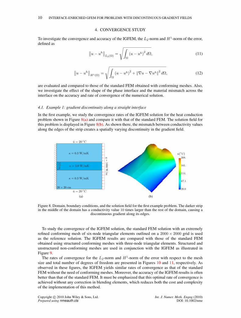
4.1. Example 1: gradient discontinuity along a straight interface

In the first example, we study the convergence rates of the IGFEM solution for the heat conductionproblem shown in Figure 8(a) and compare it with that of the standard FEM. The solution field forthis problem is displayed in Figure 8(b). As shown there, the mismatch between conductivity valuesalong the edges of the strip creates a spatially varying discontinuity in the gradient field.

3.2cm

20× 20 cm

q=

1000W

/m2

u = 20 C

u = 20 C

κ = 0.3 W/mK

κ = 0.3 W/mK

κ = 3.0 W/mK

(a)

Temperature

20.0

67.1

114.

161.

208.u(C)

(b)

Figure 8. Domain, boundary conditions, and the solution field for the first example problem. The darker stripin the middle of the domain has a conductivity value 10 times larger than the rest of the domain, causing a

discontinuous gradient along its edges.

To study the convergence of the IGFEM solution, the standard FEM solution with an extremelyrefined conforming mesh of six-node triangular elements outlined on a 2000× 2000 grid is usedas the reference solution. The IGFEM results are compared with those of the standard FEMobtained using structured conforming meshes with three-node triangular elements. Structured andunstructured non-conforming meshes are used in conjunction with the IGFEM as illustrated inFigure 9.

The rates of convergence for the L2-norm and H1-norm of the error with respect to the meshsize and total number of degrees of freedom are presented in Figures 10 and 11, respectively. Asobserved in these figures, the IGFEM yields similar rates of convergence as that of the standardFEM without the need of conforming meshes. Moreover, the accuracy of the IGFEM results is oftenbetter than that of the standard FEM. It must be emphasized that this optimal rate of convergence isachieved without any correction in blending elements, which reduces both the cost and complexityof the implementation of this method.


11

(a) (b) (c)

Figure 9. Three different types of meshes used for the numerical solutions in the first example problem:(a) structured conforming mesh for the standard FEM solution, (b) structured and (c) unstructured non-

conforming meshes for the IGFEM solution.

IGFEM: structured

IGFEM: unstructured Standard FEM

0.002 0.0040.003

0.03

0.3

0.020.01h

21

u−

uh L

2(Ω

)

(a)

IGFEM: structured


10

1

1

20

0.002 0.020.01

30

50

70

0.004

u−

uh H

1(Ω

)

h(b)

Figure 10. Convergence rates in L2-norm and H1-norm of the error with respect to the mesh size (h) for the

example problem shown in Figure 8. IGFEM results are obtained using structured and unstructured meshessimilar to those shown in Figure 9.

4.2. Example 2: Curved interfaces and effect of material mismatch

The use of conforming meshes in problems with curved interfaces solved with the standard FEMdoes not usually yield optimal rate of convergence due to the geometry approximation error.



IGFEM: structured


11

100 70003000300 10000.003

0.03

0.3

u−

uh L

2(Ω

)

ndof

(a)

IGFEM: structured


10

0.51

20

100 70003000

30

50

70

300 1000ndof

u−

uh H

1(Ω

)

(b)

Figure 11. Convergence rates in L2-norm and H1-norm of the error with respect to the total number of dofs

(ndof ) for the example problem shown in Figure 8.

Similarly, we do not expect to achieve the optimal rate of convergence for such problems usingthe IGFEM. Instead, the goal here is to compare the performance of the IGFEM with that of thestandard FEM to determine the efficiency of this method for handling such problems. The effectof the material mismatch, i.e., the ratio of the thermal conductivity values across the interface, onthe performance of the IGFEM is another issue studied in this example. It has been shown that theaccuracy of conventional GFEM deteriorates when the conductivity mismatch increases and furthercorrections are necessary to achieve the optimal rate of convergence [33].

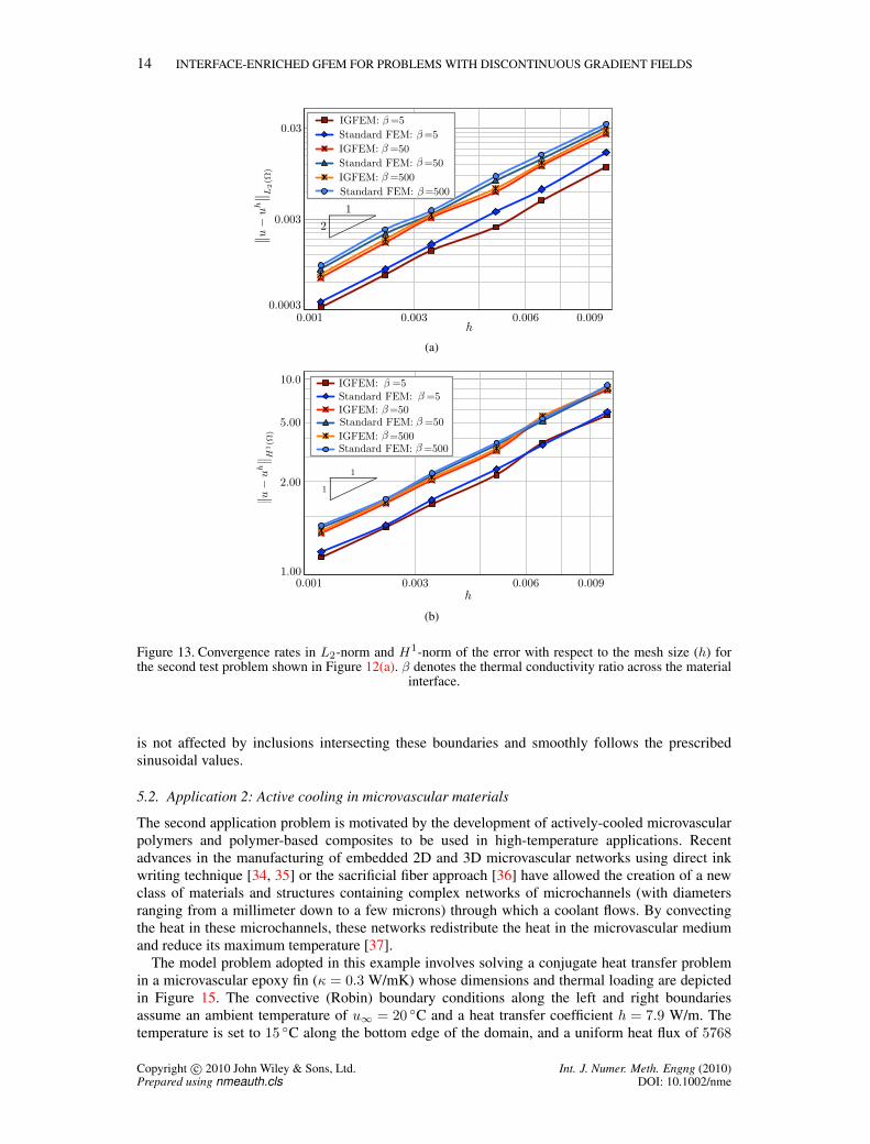
The domain and boundary conditions for the second example problem are depicted in Figure12(a). The material mismatch values are investigated corresponding to three values of the thermalconductivity ratio β = κi/κm = 5, 50, and 500 where κi and κm refer to the thermal conductivity ofthe inclusion and matrix, respectively. The corresponding thermal fields obtained with the IGFEMon a 40× 40 unstructured non-conforming mesh are presented in Figures 12(b), 12(c), and 12(d),respectively, showing the ability of the IGFEM to capture the increasing gradient discontinuityacross the interface.

Since no exact solution is available for this problem, a standard FEM solution obtained with ahighly refined conforming mesh of ten-node triangular elements is used as the reference solution.The convergence rates for the L2-norm and H1-norm of the error for the standard FEM and IGFEMsolutions are presented in Figure 13 for the three values of mismatch ratio α. As shown in this figure,the accuracy and convergence rates of the IGFEM solutions are similar and in some cases better than


13

20× 20 cmu = 20 C

14 cm

q = 500 W/m2

κ = 0.3 W/mK

κ = 1.5, 15, or 150 W/mK

(a)

230.

20.020.0

72.472.4

125.

177.177.

u(C)

(b)

Temperature

20.0

62.5

105.

148.

190.u(C)

(c)

Temperature

20.0

61.5

103.

144.

186.u(C)

(d)

Figure 12. (a) Domain geometry and boundary conditions of the second example problem. The circularinclusion has a larger conductivity (κi) than the rest of the domain (κm). (b) Temperature field for

α = κi/κm = 5, (c) 50, and (d) 500.

the corresponding results obtained with the standard FEM. It should also be noted that, without anycorrection, the performance of the IGFEM does not deteriorate as the conductivity values across theinterface increases.

5. APPLICATIONS

In this section, we apply the IGFEM to solve two thermal problems with gradient discontinuity. Weuse these applications to address issues such as assigning Dirichlet boundary conditions at elementsintersecting with the interface and conjugate heat transfer problems.

5.1. Application 1: Heterogeneous material with multiple circular inclusions

The test problem shown in Figure 14(a) can be considered as a model problem for heat transfer inheterogeneous materials. Prescribed temperature boundary conditions with sinusoidal variations areconsidered along the top and bottom edges of the domain, while a constant heat flux is applied tothe sides.

The IGFEM solution field shown in Figure 14(b) is obtained with a 120× 80 non-conformingstructured mesh of three-node triangular elements. The gradient discontinuity at material interfacescan be clearly distinguished in the IGFEM solution. As shown in Figure 14(a), some of theinclusions intersect the domain boundary with prescribed values of temperature. As discussed earlierin Section 3, assigning Dirichlet boundary conditions at nodes of the enriched elements in theIGFEM is similar to that of the standard FEM and requires no special modifications. Figure 14(b)clearly illustrates that the solution field along the boundaries with prescribed values of temperature



IGFEM: =5 Standard FEM: =5 IGFEM: =50 Standard FEM: =50 IGFEM: =500 Standard FEM: =500

0.001 0.0030.0003

0.003 21

0.03

0.0090.006

ββ

ββ

ββ

h

u−

uh L

2(Ω

)

(a)

IGFEM: =5 Standard FEM: =5IGFEM: =50Standard FEM: =50IGFEM: =500 Standard FEM: =500

0.001 0.0031.00

2.00 1

1

5.00

10.0

0.0090.006

ββ

ββ

ββ

u−

uh H

1(Ω

)

h(b)

Figure 13. Convergence rates in L2-norm and H1-norm of the error with respect to the mesh size (h) for

the second test problem shown in Figure 12(a). β denotes the thermal conductivity ratio across the materialinterface.

is not affected by inclusions intersecting these boundaries and smoothly follows the prescribedsinusoidal values.

5.2. Application 2: Active cooling in microvascular materials

The second application problem is motivated by the development of actively-cooled microvascularpolymers and polymer-based composites to be used in high-temperature applications. Recentadvances in the manufacturing of embedded 2D and 3D microvascular networks using direct inkwriting technique [34, 35] or the sacrificial fiber approach [36] have allowed the creation of a newclass of materials and structures containing complex networks of microchannels (with diametersranging from a millimeter down to a few microns) through which a coolant flows. By convectingthe heat in these microchannels, these networks redistribute the heat in the microvascular mediumand reduce its maximum temperature [37].

The model problem adopted in this example involves solving a conjugate heat transfer problemin a microvascular epoxy fin (κ = 0.3 W/mK) whose dimensions and thermal loading are depictedin Figure 15. The convective (Robin) boundary conditions along the left and right boundariesassume an ambient temperature of u∞ = 20 C and a heat transfer coefficient h = 7.9 W/m. Thetemperature is set to 15 C along the bottom edge of the domain, and a uniform heat flux of 5768


15

xy

κ = 1

κ = 2

κ = 3

κ = 5

q=

300W

/m2q

=−60

0W

/m2

u(C) = 50 sin (4πx/0.12)

u(C) = 70 sin (2πx/0.12)

0.12 m

0.08m

κ = 0.3

(a)

13.5 41.8 70.0-71.2 -42.9 -14.7u(C)

(b)

Figure 14. Problem statement and solution field obtained with the IGFEM for the thermal problem in themodel heterogeneous material. The shades or colors used in the inclusions and in the matrix correspond to

prescribed values of the thermal conductivity given in W/mK.

W/m is applied along the top edge. This particular value is chosen so that the maximum temperaturealong the top edge of the domain in the absence of cooling is 150 C.

Motivated by manufacturing constraints involved in the use of the sacrificial fiber technique, weadopt a sinusoidal shape for the centerline of the microchannel with amplitude A = 3.2 mm anddiameter D = 500µm. This particular configuration of the microchannel can be effectively used inactive cooling of the domain with boundary conditions shown in Figure 15 through redistributingthe heat inside the domain. The coolant used in this study is water (κ = 0.6 W/mK, ρ = 1000kg/m3, cp = 4183 J/kgK), with an inflow temperature set at ue = 20 C and a mass flow rate m = 2g/min. Convective boundary conditions, similar to that of the surrounding matrix at the sides, isconsidered for the fluid at the outflow. Fully developed Poiseuille flow conditions are assumed inthe microchannel, with a velocity profile given by [38]



7mm

60 mm

u = 15 C

ue = 20 C

q = 5768 W/m2

500 µm

m = 2 g/min

Figure 15. Domain geometry, boundary conditions, and schematic configuration of the sinusoidalmicrochannel for the second application problem. The domain is composed of epoxy material and the fluidcirculating in the microchannels is water. The inset shows a part of the structured non-conforming mesh

used in the IGFEM solution.

|v| = 2v

1−

2r

D

2,

where v = 4m/πD2 is the average velocity of the fluid, and r is the radial distance from thecenterline.

Details of the non-conforming mesh used in this study are shown in the inset of Figure 15.The domain is discretized with a structured mesh of three-node triangular elements outline overa 360× 42 grid. The temperature field for this problem for three different wavelengthes of themicrochannel is presented in Figure 16. For the sake of clarity, the temperature profile inside themicrochannels is not shown in this figure. However, Figure 16(d) shows the temperature profilealong the line depicted in Figure 16(b) where the temperature distribution inside the microchanneland the weak discontinuity along its edges can be clearly observed.

One of the key design variables for this class of materials is the wavelength of the embeddedsinusoidal microchannel. As shown in Figure 16, the wavelength plays an important role inredistributing the heat in the component as the coolant absorbs the heat from the hot area of thedomain at the peaks of the sinusoidal curve and exchanges the heat in the colder region, i.e., bottomof the domain, achieving a substantial reduction on the maximum temperature in the polymeric fin.This reduction is especially apparent in the embedded microchannel with the smaller wavelength (tothe detriment, of course, of the additional cost of driving the fluid through a longer microchannel).It should be noted that the IGFEM is particularly well suited for this class of computational design,as the same mesh can be used to find the optimal configuration of the microvascular network.

6. CONCLUSIONS

The formulation and implementation of an interface-based GFEM scheme for solving thermalproblems in discontinuous gradient fields has been presented. Similar to conventional GFEM,this new method can be used for solving problems with gradient discontinuity without usinga conforming mesh. The unique feature of the IGFEM is that generalized dofs are assignedto the interface nodes and not to the nodes of the original FEM mesh. This variation in theformulation of the IGFEM eliminates problems encountered with some enrichment functions in theconventional GFEM for assigning Dirichlet boundary conditions at the enriched nodes. Moreover,enrichment functions in the IGFEM are simply constructed through the linear combination ofstandard Lagrangian shape functions of the integration elements, which reduces the cost and


17

(a)

A B

(b)

112.15.0 34.5Temperature

73.4 92.953.9u(C)

(c)

30

40

50

60

23.0 26.5 30.0 33.5 37.0Distance from left edge (mm)A B

Epoxy Epoxy Epoxy Epoxy

Wat

er

Wat

er

Wat

er

u(

C)

(d)

Figure 16. IGFEM solution for the second application problem presented in Figure 15: (a), (b), and (c)represent the temperature field in the actively-cooled domain for a wavelength of the microchannel of 6.13,9.23, and 13.33 mm, respectively. (d) temperature profile along the line segment AB shown in Figure (b).

The darker vertical regions denote the location of the microchannel.

facilitates the implementation of this method. It was shown that the IGFEM solutions obtainedwith non-conforming meshes achieve the same optimal rate of convergence and level of accuracy asthose of the standard FEM with conforming meshes. Moreover, unlike some GFEM formulations,the performance of the method is not deteriorated as the ratio of the material mismatch acrossthe interface increases. We also investigated the application of the IGFEM for heat transfer inheterogeneous materials and conjugate heat transfer in actively-cooled microvascular materials.

ACKNOWLEDGEMENT

This work has been supported by the Air Force Office of Scientific Research Multidisciplinary UniversityResearch Initiative (Grant No, F49550-05-1-0346). The authors wish to thank insightful discussions withProf. S. R. White, Prof. N. R. Sottos and Dr. P. R. Thakre at the University of Illinois.

REFERENCES

1. Y. S. Song and J. R. Youn. Evaluation of effective thermal conductivity for carbon nanotube/polymer compositesusing control volume finite element method. Carbon, 44(4):710–717, 2006.

2. X. F. Wang, G. M. Zhou X. W. Wang, and C.W. Zhou. Multi-scale analyses of 3D woven bomposite based onperiodicity boundary conditions. Journal of Composite Materials, 41(14):1773–1788, 2007.

3. M. Iuga and F. Raether. FEM simulations of microstructure effects on thermoelastic properties of sintered ceramics.Journal of the European Ceramic Society, 27:511–516, 2007.



4. L. A. Shipton. Thermal management applications for microvascular systems. Master’s thesis, University of Illinoisat Urbana-Champaign, 2007.

5. Z. Yue and D. H. Robbins Jr. Adaptive superposition of finite element meshes in non-linear transient solidmechanics problems. International Journal for Numerical Methods in Engineering, 72:1063–1094, 2007.

6. J. Canales, J.A. Tarrago, and A. Hernindez. An adaptive mesh refinement procedure for shape optimal design.Advances in Engineering Software, 18:131–145, 1993.

7. C. A. Duarte and T. J. Oden. H-p clouds - an h-p meshless method. Numerical Methods for Partial Differential

Equations, 12(6):673–705, 1996.8. T. J. Oden, C. A. Duarte, and O. C. Zienkiewicz. A new cloud-based hp finite element method. Computer Methods

in Applied Mechanics and Engineering, 153(1-2):117–126, 1998.9. J. M. Melnek and I Babuska. The partition of unity finite element method: Basic theory and applications. Computer

Methods in Applied Mechanics and Engineering, 139(1-4):289–314, 1996.10. I. Babuska and J. M. Melnek. The partition of unity method. International Journal for Numerical Methods in

Engineering, 40(4):727–758, 1997.11. C. A. Duarte, O. N. Hamzeh, T. J. Liszka, and W. W. Tworzyldo. A generalized finite element method for

the simulation of three-dimensional dynamic crack propagation. Computer Methods in Applied Mechanics and

Engineering, 190(15-17):2227–2262, 2001.12. T. Belytschko and T. Black. Elastic crack growth in finite elements with minimal remeshing. International Journal

for Numerical Methods in Engineering, 45(5):601–620, 1999.13. N. Moes, J. Dolbow, and T. Belytschko. A finite element method for crack growth without remeshing. International

Journal for Numerical Methods in Engineering, 46(1):131–150, 1999.14. J. Dolbow, N. Moes, and T. Belytschko. Discontinuous enrichment in finite elements with a partition of unity

method. Finite Elements in Analysis and Design, 36:235–260, 2000.15. N. Sukumar, N. Moes, B. Moran, and T. Belytschko. Extended finite element method for three-dimensional crack

modeling. International Journal for Numerical Methods in Engineering, 48:1549–1570, 2000.16. N. Moes and T. Belytschko. Extended finite element method for cohesive crack growth. Engineering Fracture

Mechanics, 69:813–833, 2002.17. J. Mergheim, E. Kuh, and P. Steinmann. A finite element method for the computational modeling of cohesive

cracks. International Journal for Numerical Methods in Engineering, 63:276–289, 2005.18. E. Samaniego and T. Belytschko. Continuum-discontinuum modeling of shear bands. International Journal for

Numerical Methods in Engineering, 62:1857–1872, 2005.19. J. H. Song, P. M. A. Areias, and T. Belytschko. A method for dynamic and shear band propagation with phantom

nodes. International Journal for Numerical Methods in Engineering, 67:868–893, 2006.20. A. R. Khoei and M. Nikbakht. Contact friction modeling with the extended finite lement method (X-FEM). Journal

of Material Science Technology, 177:58–62, 2006.21. J. Fish and Z. Yuan. Multiscale enrichment based on partition of unity. International Journal for Numerical

Methods in Engineering, 62:1341–1359, 2005.22. G. J. Wagner, S. Ghosal, and W. K. Liu. Particulate flow simulations using lubrication theory solution enrichment.

International Journal for Numerical Methods in Engineering, 56:1261–1289, 2003.23. J. Chessa and T. Belytschko. An enriched finite element method and level sets for axisymetric two-phase flow with

surface tension. International Journal for Numerical Methods in Engineering, 58:2041–2064, 2003.24. N. Sukumar, Z. Hang, J. H. Prevost, and Z. Suo. Partition of unity enrichment for bimaterial interface cracks.

International Journal for Numerical Methods in Engineering, 59:1075–1102, 2004.25. A. M. Aragon, C. A. Duarte, and P. H. Geubelle. Generalized finite element enrichment functions generalized finite

element enrichment functions for discontinuous gradient fields. International Journal for Numerical Methods in

Engineering, 82:242–268, 2010.26. N. Moes, M. Cloirec, P. Cartraud, and J. F. Remacle. A computational approach to handle complex microstructure

geometries. Computer Methods in Applied Mechanics and Engineering, 192:3163–3177, 2003.27. N. Moes, E. Bechet, and M. Tourbier. Imposing Dirichlet boundary conditions in the extended finite element

method. International Journal for Numerical Methods in Engineering, 67(12):1641–1669, 2006.28. I. Babuska, U. Banerjee, and O. JE. Survey of meshless and generalized finite element methods: A unified approach.

Acta Numerica, 12:1–125, 2003.29. T. P. Fries. A corrected XFEM approximation without problems in blending elements. International Journal for

Numerical Methods in Engineering, 75(5):503–532, 2008.30. T. Strouboulis, I. Babuska, and K. Copps. The design and analysis of the generalized finite element method.

Computer Methods in Applied Mechanics and Engineering, 181:43–69, 2000.31. O. C. Zienkiewicz, R. L. Taylor, and J. Z. Zhu. The finite element method: its basis and fundamentals. Elsevier,

2005.32. Z. Li, T. Lin, and X. Wu. New cartesian grid methods for interface problems using the finite element formulation.

Numerische Mathematik, 96:61–98, 2003.33. K. R. Srinivasan, K. Matous, and P. H. Geubelle. Generalized finite element method for modeling nearly

incompressible bimaterial hyperelastic solids. Computer Methods in Applied Mechanics and Engineering,197:4882–4893, 2008.

34. K. S. Toohey, N. R. Sottos, J. A. Lewis, J. S. Moore, and S. R. White. Self-healing materials with microvascularnetworks. Nature Materials, 6:581–585, 2007.

35. S. C. Olugebefola, A. M. Aragon, C. J. Hansen, A. R. Hamilton, B. D. Kozola, W. Wu, P. H. Geubelle, J. A. Lewis,N. R. Sottos, and S. R. White. Polymer microvascular network composite. Journal of Composite Materials, 44(22),2010.

36. A. P. Golden and J. Tien. Fabrication of microfluidic hydrogels using molded gelatin as a sacrificial element. Lab

on a Chip, 4(6):720–725, 2007.


19

37. A. M. Aragon, J. K. Wayer, P. H. Geubelle, D. E. Goldberg, and S. R. White. Design of microvascular flownetworks using multi-objective genetic algorithms. Computer Methods in Applied Mechanics and Engineering,197:4399–4410, 2008.

38. C. A. Brebbia and A. Ferrante. Computational Hydraulics. Butterworths, 1983.


Date post:	10-Apr-2018
Category:	Documents
Upload:	phungdan
View:	219 times
Download:	0 times

An interface-enriched generalized ﬁnite element method for...

Documents