An intertwined method for making low-rank,

sum-of-product basis functions that makes it possible to

compute vibrational spectra of molecules with more than

10 atoms

Phillip S. Thomas

e-mail: Phillip.Thomas@chem.queensu.ca

Tucker Carrington Jr.

e-mail: Tucker.Carrington@queensu.ca

fax: 613-533-6669

Chemistry Department, Queen’s University

Kingston, Ontario, Canada

K7L 3N6

Canada

11/21/2016

Abstract

We propose a method for solving the vibrational Schroedinger equation with which one can

compute spectra for molecules with more than ten atoms. It uses sum-of-product (SOP) basis

1

functions stored in canonical polyadic (CP) tensor format and generated by evaluating matrix-

vector products. By doing a sequence of partial optimizations, in each of which the factors in

a SOP basis function for a single coordianate are optimized. the rank of the basis functions

is reduced as matrix-vector products are computed. This is better than using an alternating

least squares method to reduce the rank, as is done in the Reduced-Rank Block Power Method

(RRBPM). Partial optimization is better because it speeds up the calculation by about an order

of magnitude and allows one to significantly reduce the memory cost. We demonstrate the

effectiveness of the new method by computing vibrational spectra of two molecules, ethylene

oxide (C2H4O) and cyclopentadiene (C5H6), with 7 and 11 atoms, respectively.

I. Introduction

Given a potential energy surface (PES), it is now rather straightforward to compute the vibrational

spectrum of a triatomic molecule using a variational method.1–3 When the PES is a sum of products

(SOP) and the basis functions are products of univariate functions, potential matrix elements are

easily obtained from products of 1D integrals that are evaluated with 1D quadrature. For a general

PES, one needs 3D quadrature to calculate potential matrix elements, but this is not difficult on any

modern computer. The Hamiltonian matrix whose eigenvalues approximate energy levels is small

enough that standard eigensolvers can be used. For four-atom, five-atom, and six-atom molecules

variational calculations are more difficult, especially for general (e.g. not SOP) PESs. Using a SOP

PES obviates the need for multidimensional quadrature, but the basis set is usually large enough

that standard eigensolvers are either costly or impossible to use. Both the CPU and the memory

costs are too high. When the memory required to store the Hamiltonian matrix is larger than the

memory of the computer, a calculation with a standard eigensolver is impossible. In this paper we

present ideas that make it possible to do variational calculations to obtain vibrational spectra of

molecules with 11 atoms. They work only if the PES is SOP. For many molecules with five or more

atoms, most available PESs are in SOP form. There are several methods for bringing a general

PES into SOP form.4–6

Probably the simplest way to overcome the memory barrier that one confronts for molecules

2

with more than three atoms is to use an iterative eigensolver.7–12 When using an iterative eigen-

solver it is necessary only to store vectors and not the Hamiltonian matrix. In fact, it is also

unnecessary to compute elements of the Hamiltonian matrix. With a direct product basis (DPB),

the size of the vectors is nD, where n is the number of basis functions for a single coordinate

and D is the number of coordinates. Unfortunately, in the six-atom case, even storing vectors is

impossible. One way to deal with the problem is to prune the direct product basis.1,3,13–15 If, for

example, only basis functions are retained that satisfy n1+n2+ · · ·+nD ≤ n−1 then the size of the

vectors (basis) is reduced from nD to (D+n−1)!D!(n−1)! . Although this reduction is substantial, the memory

required is still large for molecules with 10 or more atoms. There are vibrational coupled cluster

methods that use a basis of selected product functions that have some of the same advantages

as pruned basis methods.16

We have recently shown that it is possible to use a DPB in conjunction with an iterative eigen-

solver without needing to store nD numbers to represent each vector.17–20 This is done by forcing

every basis function to be a SOP,

Ψ (q1, . . . , qD) 'n1∑i1=1

· · ·nD∑iD=1

Fi1,...,iD

D∏c=1

ϕcic (qc) , (1)

where c labels a single coordinate, and

Fi1,...,iD =

R∑r=1

sFr

D∏c=1

f(r,c)ic

. (2)

is a tensor of basis coefficients. In mathematical language, it is a tensor in CP-format and R is

called the rank.21 The memory cost of storing Fi1,...,iD is RnD, which scales linearly and not

exponentially with D. Wavefunctions are obtained by projecting into the space spanned by a set of

such SOP basis functions. Storing basis functions and wavefunctions in CP-format eliminates the

memory problem that one encounters when trying to compute vibrational spectra of molecules with

6,7... atoms. In practice, we impose a rank, R, and find that with R between 10 and 100 we are

able to obtain accurate solutions to the Schroedinger equation for molecules with fewer than eight

3

atoms. These ideas were implemented in the Reduced-Rank Block Power Method (RRBPM),

which uses a shifted power method to generate the Fi1,...,iD . With the RRBPM it is possible to

compute the lowest 70 eigenstates of CH3CN using less than 1 GB of memory. There are also

multiconfiguration time-dependent Hartree methods for computing vibrational spectra.22–25 They

also use a tensor format to store basis vectors, however, it is a direct product (or Tucker) format

and although the 1D basis functions are optimized the memory cost scales exponentially with D.

The CP format has also been used to reduce the memory cost of storing vectors in a vibrational

coupled cluster (VCC) calculation.26,27 However, it has not yet been possible to devise a VCC

algorithm, in which, like the RRBPM, all vectors are directly computed in CP format, and that

therefore requires storing only vectors in CP format and exploits its advantages to reduce CPU

cost.

One shortcoming of the RRBPM is that the shifted power method converges slowly, requiring

> 1000 iterations (i.e. matrix-vector products (MVPs) for each vector in the block) to achieve mod-

erate accuracy for a six-atom molecule such as CH3CN. The slow convergence can be mitigated

in several ways. One way is to do separate calculations for different symmetries.19 A second way is

to replace the shifted power method with an iterative eigensolver that converges more quickly.20,28

A third way is to arrange the coordinates of the molecule into groups in a tree structure and to

build the basis hierarchically by solving eigenproblems for subsets of the coordinates.18 This last

strategy, known as the Hierarchical (H-) RRBPM, uses an RRBPM to compute eigenstates at each

node of the tree. With a good choice of tree, the H-RRBPM is orders-of-magnitude faster than the

ordinary RRBPM. Importantly, since the H-RRBPM also uses the shifted power method, typically

fewer than 100 iterations are needed to converge the basis functions of a given node, with con-

vergence being slowest at the top node of the tree where the energy spectrum is densest. The

H-RRBPM could be used in combination with either of the previous two strategies. Rakhuba and

Oseledets have recently proposed a method that, like the RRBPM, builds a basis by evaluating

matrix-vector products and reducing the rank of output vectors.28 Rather than using CP format,

they opt for another tensor format. It is known as tensor-train to mathematicians and as matrix-

product states (MPS) to physicists and chemists. Rather than the power method they use inverse

4

iteration, which converges more quickly. Because it uses MPS their method has some of the fea-

tures of the density matrix renormalization group approach, but it, like the RRBPM, builds a basis

rather than optimizing a parameterized wavefunction.

The RRBPM, whether applied to the full problem or at the top node of an H-RRBPM tree,

has two other important shortcomings. The most severe is the cost of the rank reduction. After

each matrix-vector product, one must reduce the rank of the output vector. To do this, we used

an implementation of the Alternating Least Squares (ALS) algorithm similar to the one proposed

by Beylkin.29 In previous calculations most of the CPU time (typically > 90%) was spent on rank

reduction. Much less severe, but potentially important for molecules with dozens of atoms or if

one is using a desktop computer with less than 32 GB of memory, is the memory cost of storing

large-rank vectors. Storing a vector before its rank is reduced requires storing RnD numbers.

For molecules studied previously (acetonitrile, ethylene oxide), for which the SOP PES has only

hundreds of terms, this was not a problem. However, if MVPs for different vectors in the block are

evaluated on different processors, then for larger molecules the memory cost might be a problem.

The largest rank (R) usually obtained in an RRBPM calculation is a product of the rank specified

for the basis vectors (Rψ) and the number of terms in the SOP PES (T ) which might be T ∼ 10000.

If R = Rψ ∗ 10000 and Rψ = 100 and D = 50 and n = 20 then ∼ 6 GB are required to store one

vector.

In this paper we modify the RRBPM to reduce its CPU cost. In the original RRBPM, after

generating a tensor Gi1,...,iD

Gi1,...,iD =

RG∑r=1

sGr

D∏c=1

g(r,c)ic

. (3)

from input vector inFi1,...,iD by evaluating a MVP (here, the rank of G is T ∗ Rψ, where T is the

number of terms in the shifted Hamiltonian), one applies ALS to reduce its rank. ALS optimizes

outf(r,c)ic

so that outF i1,...,iD ∼ Gi1,...,iD , where

outF i1,...,iD =

Rψ∑r=1

outsFr

D∏c=1

outf(r,c)ic . (4)

5

Output vectors outf(r,c)ic

are determined first for c = 1 and then for c = 2, . . . , D and this cycle is

repeated NALS times to obtain a final set of outf (r,c)ic. The outf

(r,c)ic

are then re-named inf(r,c)ic and

another MVP is computed. This process is repeated for all vectors in a block and the Schroedinger

equation is projected into the basis obtained after Npow MVPs.

In this paper, each of the MVPs of the RRBPM is replaced by D MVPs. After evaluating D

MVPs for each vector in the block, we obtain a new block of vectors. After each of the D MVPs,

rather than using ALS to optimize outf(r,c)ic

for all coordinates, we optimize outf(r,c)ic

for a single

coordinate. This greatly reduces the cost of the optimization. Due to the incomplete optimization,

the individual basis vectors in the block may not be as close to eigenvectors as those of the

RRBPM. However, the energy levels we compute are more accurate because 1) the optimization

is so cheap that we can use a larger rank (Rψ); 2) even if the optimization is poor, repeated

applications of the shifted Hamiltonian will push all vectors in the block in the right direction; 3) it

is not important that individual basis vectors be close to eigenvectors, what matters is the space

spanned by the vectors in the block. We are intertwining the optimization of outf (r,c)icfor coordinates

c = 1, 2, . . . , D with the evaluation of MVPs.

The intertwining has three advantages. First, fewer systems of linear equations must be solved

to make the final basis. This reduces the calculation time by about an order of magnitude and

makes it possible to use larger ranks. Second, it reduces the cost of setting up the linear systems

that must be solved to do the optimizations done to make new blocks of vectors. Third, the new

method can be implemented so that there is no need to generate large-rank CP-vectors. This

considerably reduces the memory cost of calculations if a Hamiltonian with many terms is used or

if many states are computed in parallel.

6

II. Intertwining matrix-vector products with rank reduction

A. CP format and matrix-vector products

The RRBPM uses sum-of-products basis functions,

Ψ (q1, . . . , qD) 'n1∑i1=1

· · ·nD∑iD=1

Fi1,...,iD

D∏c=1

ϕcic (qc) , (5)

where ϕcic (qc) are 1-D basis functions depending on coordinate c, and

Fi1,...,iD =

Rψ∑r=1

sFr

D∏c=1

f(r,c)ic

, (6)

where each term in the sum over r is weighted by a normalization coefficient sr. We require the

Hamiltonian operator to be in sum-of products form,

H =

T∑m=1

D∏c=1

hm,c , (7)

where hm,c is an operator depending only on coordinate c. A matrix-vector product is17

(G)i′1,i′2,...i′D= (HF)i′1,i′2,...i′D

=∑

i1,i2,...iD

(T∑

m=1

D∏c′=1

hm,c′

)i′1,i′2,...i

′D;i1,i2,...iD

Rψ∑r=1

sr

D∏c=1

f(r,c)ic

=

T∑m=1

Rψ∑r=1

sr

D∏c=1

∑ic

(hm,c

)i′c,ic

f(r,c)ic

=

T∑m=1

Rψ∑r=1

sr

D∏c=1

∑ic

g(r,c)ic

. (8)

In this paper, we denote large-rank vectors G (rank� Rψ) and small-rank vectors F (rank= Rψ).

The matrix-vector product costs O(TRψn

2D)

operations.

7

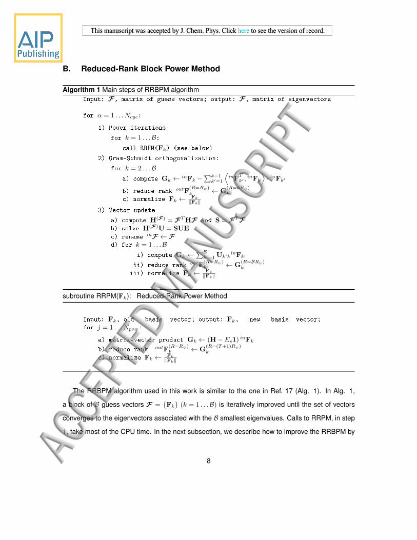
B. Reduced-Rank Block Power Method

Algorithm 1 Main steps of RRBPM algorithmInput: F, matrix of guess vectors; output: F, matrix of eigenvectors

for α = 1 . . . Ncyc:

1) Power iterations

for k = 1 . . .B:call RRPM(Fk) (see below)

2) Gram-Schmidt orthogonalization:

for k = 2 . . .Ba) compute Gk ← inFk −

∑k−1k′=1

⟨inF

Tk′ ,

inFk

⟩· inFk′

b) reduce rank outF(R=Rψ)k ← G

(R=kRψ)k

c) normalize Fk ← Fk‖Fk‖

3) Vector update

a) compute H(F) = FTHF and S = FTFb) solve H(F)U = SUEc) rename inF ← Fd) for k = 1 . . .B

i) compute Gk ←∑Bk′=1 Uk′k

inFk′

ii) reduce rank outF(R=Rψ)k ← G

(R=BRψ)k

iii) normalize Fk ← Fk‖Fk‖

subroutine RRPM(Fk): Reduced-Rank Power Method

Input: Fk, old basis vector; output: Fk, new basis vector;

for j = 1 . . . Npow:

a) matrix-vector product Gk ← (H− Es1) inFk

b) reduce rank outF(R=Rψ)k ← G

(R=(T+1)Rψ)k

c) normalize Fk ← Fk‖Fk‖

The RRBPM algorithm used in this work is similar to the one in Ref. 17 (Alg. 1). In Alg. 1,

a block of B guess vectors F = {Fk} (k = 1 . . .B) is iteratively improved until the set of vectors

converges to the eigenvectors associated with the B smallest eigenvalues. Calls to RRPM, in step

1, take most of the CPU time. In the next subsection, we describe how to improve the RRBPM by

8

intertwining RRPM steps a and b. All of the steps in Alg. 1 which generate a large-rank Gk vector

must be followed by rank-reduction and normalization. The Gk vector in the RRPM step a has rank

TRψ, whereas the Gk vectors in steps 2a and 3d-i have at most rank BRψ. We use Alternating

Least Squares (ALS)29 to reduce the rank (unless there are only two coordinates, in which case we

reduce the ranks using Singular Value Decomposition).30 The ALS procedure finds a small-rank

vector, Fk, which closely approximates a large-rank vector, Gk, by iteratively improving Fk one

coordinate at a time.

For each coordinate c, let us define the following matrices of inner products:

Bcr′,r =⟨f(r′,c),f (r,c)

⟩(9a)

P cr′,r =⟨g(r′,c),f (r,c)

⟩(9b)

B 6=cr′,r =∏c′ 6=c

Bc′

r′,r (9c)

P 6=cr′,r =∏c′ 6=c

P c′

r′,r (9d)

Br′,r =

D∏c=1

Bcr′,r (9e)

Pr′,r =

D∏c=1

P cr′,r. (9f)

Note that elements of the matrices B 6=c and P 6=c are products of inner products for all coordinates

except coordinate c. P 6=c is used to construct right-hand sides of a linear system:

b(ic,c)r =

RG∑r′=1

sGr′ g(r′,c)ic

P 6=cr′,r . (10)

The linear systems are solved for x(ic,c):

B 6=cx(ic,c) = b(ic,c) . (11)

9

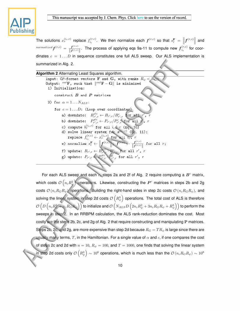
The solutions x(ic,c)r replace f

(r,c)ic

. We then normalize each f (r,c) so that sFr =∥∥∥f (r,c)

∥∥∥ and

normalizedf (r,c) = f(r,c)

‖f(r,c)‖ . The process of applying eqs 9a-11 to compute new f(r,c)ic

for coor-

dinates c = 1 . . . D in sequence constitutes one full ALS sweep. Our ALS implementation is

summarized in Alg. 2.

Algorithm 2 Alternating Least Squares algorithm.Input: CP-format vectors F and G, with ranks Rψ < RG;

Output: outF, such that ‖outF−G‖ is minimized

1) Initialization:

construct B and P matrices

2) for α = 1 . . . NALS:

for c = 1 . . . D: (Loop over coordinates)

a) downdate: B 6=cr′,r ← Br′,r/Bcr′,r for all r′, r

b) downdate: P 6=cr′,r ← Pr′,r/Pcr′,r for all r′, r

c) compute b(ic,c)r for all ic, r (Eq. 10)

d) solve linear system for x(ic,c) (Eq. 11);

replace f(r,c)ic

← x(ic,c)r for all ic, r

e) normalize sFr ←∥∥∥f (r,c)

∥∥∥; f (r,c) ← f(r,c)

‖f(r,c)‖ for all r;

f) update: Br′,r ← B 6=cr′,r ·Bcr′,r for all r′, r

g) update: Pr′,r ← P 6=cr′,r · P cr′,r for all r′, r

For each ALS sweep and each c, steps 2a and 2f of Alg. 2 require computing a Bc matrix,

which costs O(ncR

2ψ

)operations. Likewise, constructing the P c matrices in steps 2b and 2g

costs O (ncRGRψ) operations. Building the right-hand sides in step 2c costs O (ncRGRψ), and

solving the linear system in step 2d costs O(R3ψ

)operations. The total cost of ALS is therefore

O(D(ncR

2ψ + ncRGRψ

))to initialize andO

(NALSD

(2ncR

2ψ + 3ncRGRψ +R3

ψ

))to perform the

sweeps in step 2. In an RRBPM calculation, the ALS rank-reduction dominates the cost. Most

costly are the steps 2b, 2c, and 2g of Alg. 2 that require constructing and manipulating P matrices.

Steps 2b, 2c, and 2g, are more expensive than step 2d because RG = TRψ is large since there are

usually many terms, T , in the Hamiltonian. For a single value of α and c, if one compares the cost

of steps 2c and 2d with n = 10, Rψ = 100, and T = 1000, one finds that solving the linear system

in step 2d costs only O(R3ψ

)∼ 106 operations, which is much less than the O (ncRGRψ) ∼ 108

10

operations required to build the right hand sides in step 2c. Moreover, as the number of atoms

in the molecule increases, we expect T to increase faster than Rψ (the number of quartic terms

scales as D4), which means that ALS steps 2b, 2c, and 2g will dominate the cost of using the

RRBPM on large molecules.

C. Intertwining: Reducing the cost by using partial optimization

In the call to RRPM in step 1 of Alg. 1, each vector is replaced with a new vector obtained by

repeating the ALS procedure Npow times. Each call to RRPM requires making P 6=c matrices and

the right hand sides b(ic,c) (eq. 10) after every MVP and solving linear equations NpowNALSD

times for each vector and this is costly. In this paper we use a modified version of the RRBPM

(Alg. 1) where the call to the RRPM in step 1 is replaced with Alg. 3. In Alg. 3, for each α, we

calculate a new vector, obtained after completion of the loop over c, by evaluating D MVPs and

after each of them, rather than using the ALS to optimize outf(r,c)ic

for all coordinates, we optimize

outf(r,c)ic

for a single coordinate. What we call a “sweep" is completed when the outf (r,c) for all

the coordinates have been replaced. In terms of equations, for c = c′, the shifted Hamiltonian is

applied to a small-rank vector

inFi1,...,iD =

Rψ∑r=1

D∏c=1

inf(r,c)ic

(12)

to make a large-rank vector

Gi1,...,iD =

RG∑r′=1

D∏c=1

g(r′,c)ic

. (13)

which is replaced with a small-rank vector

outFi1,...,iD =

Rψ∑r=1

D∏c=1

outf(r,c)ic

, (14)

where for all c except c = c′, outf(r,c)ic

= inf(r,c)ic

. The key idea is that outFi1,...,iD is not fully

optimized.

The most important feature of Alg. 3 is that after every MVP f (r,c) is updated only for one value

11

of c and therefore to evaluate the next MVP it is only necessary to compute g(r′,c) = hm,cf(r,c)

for one value of c. Steps 2a-e improve the set of f vectors for coordinate c; in step 2f one mul-

tiplies the new f (r,c) with a 1D matrix in order to update g(r′,c). Because f (r,c) is updated only

for one c, there is no need to compute B and P matrices after completing one sweep before

beginning another. In Alg. 1, the g(r′,c) are replaced in batches, i.e. after each MVP all of

the g(r′,c) are modified. In Alg. 3 the g(r′,c) are sequentially replaced in a rolling fashion, i.e.

g(r′,c=1), g(r′,c=2), . . . , g(r′,c=D); g(r′,c=1), g(r′,c=2), . . . , g(r′,c=D); . . ., etc.

Alg. 3 has several important advantages. First, to make a final basis vector, it requires solving

linear equations only NsweepD times (with Nsweep ≈ Npow in Alg. 1) and thereby reduces the

number of linear solves by a factor of NALS . In previous papers, we used values of NALS between

10 and 100. Second, Alg. 3 significantly reduces the initialization cost because one needs to

compute B and P matrices from scratch only once (at the beginning of a cycle), before entering

the loop over α in step 2. By contrast, in the call to RRPM of Alg. 1, one must compute B and P

from scratch for each value of j, at the beginning of ALS. Third, after optimizing f (r,c)icfor coordinate

c in Alg. 3, evaluating a MVP requires changing only g(r′,c); g(r′,c′) with c′ 6= c are re-used. This

reduces the cost of the MVPs because in the RRBPM, each time ALS is used, all of the g(r′,c)ic

are

re-computed.

A better optimization might speed up convergence, but it is not necessary and would be costly.

When α is small, there is certainly no need for an excellent optimization because Gi1,...,iD itself

may be a poor basis vector (i.e. far from an eigenvector). When α is large, there might be some

advantage to doing an excellent optimization because Gi1,...,iD itself is a better basis vector (i.e.

close to an eigenvector). Despite the partial optimization of Alg. 3, each time we apply the shifted

Hamiltonian we drive the space spanned by basis vectors toward the space spanned by the B

eigenvectors with the smallest eigenvalues. The partial optimization of outFi1,...,iD introduces noise

into the basis vectors, which slows convergence, but one can compensate for it by increasing the

rank (Rψ) of outFi1,...,iD .

12

Algorithm 3 Intertwined power method.Input: vector in block, F, with rank RF

Output: improved vector in block, F, with rank RF

1) Initialization:

a) compute matrix-vector product: (H− Es1)F = Gb) construct B and P matrices

2) for α = 1 . . . Nsweep:

for c = 1 . . . D: (Loop over coordinates)

a) downdate: B 6=cr′,r ← Br′,r/Bcr′,r for all r′, r

b) downdate: P 6=cr′,r ← Pr′,r/Pcr′,r for all r′, r

c) compute b(ic,c)r for all ic, r (Eq. 10)

d) solve linear system for x(ic,c) (Eq. 11);

replace f(r,c)ic

← x(ic,c)r for all ic, r

e) normalize sFr ←∥∥∥f (r,c)

∥∥∥; f (r,c) ← f(r,c)

‖f(r,c)‖ for all r;

if c = D: normalize F← F‖F‖

f) update MVP:

for m = 1 . . . T:

for l = 1 . . . Rψ:

r′ ← (m− 1)Rψ + l

g(r′,c) ← sFl hm,cf(l,c)

g) update: Br′,r ← B 6=cr′,r ·Bcr′,r for all r′, r

h) update: Pr′,r ← P 6=cr′,r · P cr′,r for all r′, r

13

The cost per vector is

O(Npow

(TRn2D +D

(ncR

2ψ + ncRGRψ

)+NALSD

(2ncR

2ψ + 3ncRGRψ +R3

ψ

)))for the ordinary power method, but only

O(TRn2D +D

(ncR

2ψ + ncRGRψ

)+NsweepD

(2ncR

2ψ + 3ncRGRψ +R3

ψ + TRn2))

for the intertwined power method. The intertwined algorithm essentially reduces the cost by a

factor of NALS compared to the ordinary power method. In addition, it only requires one to buildB

and P from scratch once per call, in contrast to RRPM, which builds B and P from scratch Npow

times per call, where Npow ∼ 10.

D. Avoiding large-rank vectors

Both the RRBPM and the intertwined RRBPM (I-RRBPM) of Alg. 3 store, in memory, large-rank

vectors Gi1,...,iD (see Eq. (3)). This is done by simultaneously storing all the g(r,c)ic. There are three

types of large-rank vectors: vectors generated by computing a MVP, vectors created when Gram-

Schmidt (GS) is applied to F , and vectors one obtains from the vector update step. The rank of

the first type is largest. It is RG = TRψ and because the number of terms in the Hamiltonian is

large when D is large, the memory cost of storing Gi1,...,iD of the first type can limit the size of the

molecule to which one can apply the RRBPM or I-RRBPM. The memory cost of storing the other

two types is lower. Parallelizing by computing different vectors in the block on different processors

exacerbates the problem because it increases the number of Gk vectors that must be stored. To

parallelize we use OPENMP. It would be nice to be able to compute spectra of molecules with

about 10 atoms on a standard desktop computer. This is possible with the low-memory I-RRBPM

of this section. The algorithm that avoids large-rank vectors generated by the MVPs is summarized

in Alg. 4.

To use the I-RRBPM idea one must modify f (r,c)icsequentially for c = 1, 2, . . . , D. This is done

14

by solving a system of linear equations for each c. To make the linear system one must compute,

sequentially for each c, the RHS b(ic,c)r and the matrix B 6=cr′,r. A simple way to make B 6=cr′,r is to keep

Br′,r in memory and, to build B 6=cr′,r, by dividing out (called downdating in Alg. 4) Bcr′,r and then after

modifying f (r,c)ic, update Br′,r by multiplying by the modified Bcr′,r. This is implemented in steps 2a

and 2e of Alg. 4. Making B 6=cr′,r does not require much memory because it does not involve g(r′,c)ic

.

One has to be more careful when making a RHS b(ic,c)r because it depends on all the g(r′,c)

ic(see

Eq. (10)) and it is the memory cost of storing all the g(r′,c)ic

that may be large. b(ic,c)r is calculated

in Alg. 5. To avoid storing all the g(r′,c)ic

, we calculate g(r′,c)ic

and P 6=cr′,r and sum their products, one

r′ at a time. P 6=cr′,r is calculated from Pr′,r by dividing out P cr′,r which in turn is made from g(r′,c)ic

.

After the contribution from a particular value of r′ has been added, g(r′,c)ic

is discarded. It is only

necessary to store Pr′,r. Alg. 5 requires evaluating a 1D MVP for each r′. To update in Alg. 6,

one needs P cr′,r for all r′ and because we do not store g(r′,c)ic

for all r′, these must be calculated.

That requires a second 1D MVP for each r′. In the initialization step of Alg. 4, P is computed by

multiplying P c for c = 1 . . . D (Eq. ??. This is accomplished without generating large-rank vectors

by defining P 0r′,r ≡ 1 for all r′, r, and calling Alg. 6 D times, once for each value of c.

Algorithm 4 Intertwined power method, low-memory version.Input: vector in block, F, with rank RF

Output: improved vector in block, F, with rank RF

1) Initialization:

construct B and P matrices

2) for α = 1 . . . Nsweep:

for c = 1 . . . D: (Loop over coordinates)

a) downdate: B 6=cr′,r ← Br′,r/Bcr′,r for all r′, r

b) Call Alg. 5 to calculate P 6=cr′,r for all r′, r;

and b(ic,c)r for all ic, r (Eq. 10)

c) solve linear system for x(ic,c) (Eq. 11);

replace f(r,c)ic

← x(ic,c)r for all ic, r

d) normalize sFr ←∥∥∥f (r,c)

∥∥∥; f (r,c) ← f(r,c)

‖f(r,c)‖ for all r;

if c = D: normalize F← F‖F‖

e) update: Br′,r ← B 6=cr′,r ·Bcr′,r for all r′, rf) Call Alg. 6 to compute Pr′,r for all r′, r

15

Algorithm 5 Pseudo-code for downdating P matrices and computing right-hand sides b(ic,c) with-out generating a long vector G.

Input: CP-format vector, F, with rank RF, matrix POutput: matrix P 6=c, where P 6=cr′,r = Pr′,r/P

cr′,r; right-hand sides, b(ic,c)

Initialize b(ic,c)r ← 0 for all ic, r

for m = 1 . . . T:

for l = 1 . . . Rψ:

r′ ← (m− 1)Rψ + l

g(r′,c) ← hm,cf(l,c)

for r = 1 . . . Rψ:

P 6=cr′,r ← Pr′,r/⟨g(r′,c),f (r,c)

⟩b(ic,c)r ← b

(ic,c)r + sFl g

(r′,c)ic

P 6=cr′,r for all ic

discard g(r′,c)

The cost of Algs. 4-6 isO(D(ncR

2ψ + ncRGRψ + TRn2

)+NsweepD

(2ncR

2ψ + 3ncRGRψ +R3

ψ + 2TRn2))

,

where RG = TRψ. This is less efficient than the ordinary intertwined power method in Alg. 3. In

Alg. 3, only one MVP is computed for each α, c pair in step 2f. In Alg. 4, two MVPs are needed

per α, c pair; they are evaluated in the calls to Alg. 5 and Alg. 6 in steps 2b and 2f, respectively.

The factor of 2 in the term 2TRn2 above is due to the cost of the extra MVP. The memory cost

of the low-memory intertwined power method is dominated by storing the P matrix, which costs

O(TR2

ψ

). This is less than the full-memory version of the intertwined power method, which stores

Algorithm 6 Pseudo-code for updating P 6=c matrices without generating a long vector G.

Input: CP-format vector, F, with rank RF, matrix P 6=c

Output: matrix P , where Pr′,r = P 6=cr′,r · P cr′,rfor m = 1 . . . T:

for l = 1 . . . Rψ:

r′ ← (m− 1)Rψ + l

g(r′,c) ← hm,cf(l,c)

for r = 1 . . . Rψ:

Pr′,r ← P 6=cr′,r ·⟨g(r′,c),f (r,c)

⟩discard g(r′,c)

16

P in addition to the Gk vector.

Calculating H(F) = FTHF to update vectors (step 3a in Alg. 1) also involves computing

large-rank Gk vectors with rank TRψ. Not only is it expensive to store Gk = HFk but it is also

expensive to compute the inner products 〈Fk′ ,Gk〉 needed to obtain the elements of H(F). To

reduce the memory cost in this step, we use ALS (Alg. 2), but implement it without computing or

storing large-rank vectors Gk. To do this we re-calculate g(r′,c)ic

, which requires storing f (r,c)icand

doing 1D MVPs to update, downdate, and compute RHSs. The updating is done with Alg. 6 and

the downdate and RHS calculation is done with Alg. 5. In Alg. 5 the RHSs are again obtained by

(see Eq. (10)) summing terms one r′ at a time.

We avoid also storing the Gk created during the the Gram-Schmidt and Vector Update phases

(steps 2 and 3 in Alg. 1, respectively). The memory cost of storing these Gk vectors is lower

than those obtained by evaluating MVPs because steps 2 and 3 in Alg. 1 generate vectors with

maximum rank of BRψ, but it can still be significant if the block size is large. It is possible to

implement ALS so that it is not necessary to store Gk vectors in order to compute outFk. To

perform a Gram-Schmidt orthogonalization we want

outFk ≈ Gk = inFk −k−1∑k′=1

⟨inF

T

k′ ,inFk

⟩· inFk′ (15)

and to perform a Vector Updates we want

outFk ≈ Gk =

B∑k′=1

Uk′kinF

old

k′ .

In both cases we can make outFk without building Gk. For a single c, to calculate outf(r,c)k , one

needs B 6=c and the RHS b(ic,c). The memory cost of computing B 6=c is low because it does not

require g(r′,c)ic

. To use Eq. (10) to compute b(ic,c), it is not necessary to store all the g(r′,c)ic

because

contributions for each r′ can be added to the sum and then discarded. The factors in the terms of

the vector to be reduced are f(r′,c)ic

, that are already stored, multiplied by numerical coefficients.

In the GS case, these coefficients are inner products of inFk vectors. In the vector update case,

17

the coefficients are elements of U. The coefficients are multiplied with the f(r′,c)ic

factors for the

first (c = 1) coordinate when we construct the RHS b(ic,c) vectors of the linear system.

III. Results and Discussion

In this section we report vibrational energy levels of two molecules computed using a combination

of the intertwining idea of the previous section and the H-RRBPM18 that we refer to as the Hier-

archical Intertwined Reduced-Rank Block Power Method (HI-RRBPM). All calculations described

below use the fast version (Alg. 3) instead of the low-memory version (Alg. 4). We use the in-

tertwined power method only for nodes in the tree with D > 2. For nodes with D = 2, we use

the ordinary power method with SVD to reduce the rank since SVD reduction is faster and more

accurate than any ALS-type method. As in previous papers, we parallelize over vectors in the

blocks, although other parallelization schemes are possible. Energy levels tend to decrease as

more matrix-vector products are computed and in general increasing the rank decreases levels.

However, as noted previously,20 if the rank is small energy levels oscillate. As a consequence, it is

not always true that every level decreases when the rank is increased.

The potential energy surfaces we use are “semi-diagonal” quartic Taylor expansions of the

potential about the minimum energy geometry.31 This simple form of the potential is convenient to

use, although our method is compatible with any sum-of-products potential. The Hamiltonian is

H =ωc2

(D∑c=1

− ∂2

∂q2c+ q2c

)

+1

6

D∑c1=1

D∑c2=1

D∑c3=1

φ(3)c1c2c3qc1qc2qc3

+1

24

D∑c1=1

D∑c2=1

D∑c3=1

D∑c4=1

φ(4)c1c2c3c4qc1qc2qc3qc4 , (16)

where we neglect all πtµπ terms in the KEO and the potential-like∑α µα,α term.32 In our calcula-

18

tions, the 1D basis functions, ϕcic (qc) in Eq. (5) are eigenfunctions of 1D cut Hamiltonians obtained

by keeping only the ωc/2p2c term in the KEO and setting qc′ = 0, c′ 6= c. These eigenfunctions are

obtained by solving each 1D cut Hamiltonian in a harmonic oscillator basis chosen large enough

to converge the levels of interest.

A. Ethylene oxide (C2H4O)

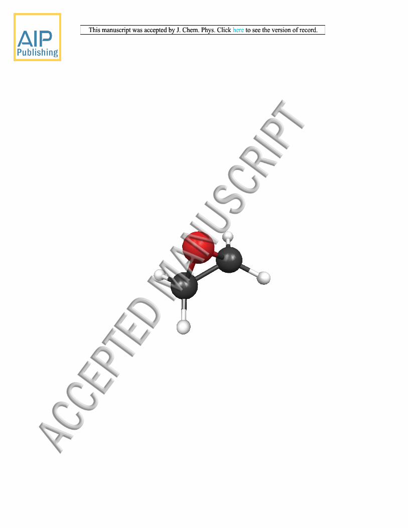
We test the HI-RRBPM by computing the lowest 200 vibrational states of the ethylene oxide (EO)

molecule (Fig. 1), which has 7 atoms and 15 vibrational DOF. As in our previous paper, we use

the PES of Bégué, Gouhaud, and Pouchan33 although newer potentials34–37 are available. The

harmonic frequencies of the PES of Ref. 33 were computed at the CCSD(T)/cc-pVTZ level and the

anharmonic constants at the B3LYP/6-31+G(d,p) level. We obtained the PES directly from one of

the authors (PC-C). It includes eight force constants missing from the Supplementary Material of

Ref. 33, but published in Ref. 38.

The trees used in the hierarchical calculations in this paper are shown in Figure 2. They are

different from the tree used in Ref. 18. We obtained the tree in Figure 2a by adding a layer (third

from the top) to the tree used earlier (Figure 11 in Ref. 18) and by increasing the basis sizes slightly

on the second-to-highest layer. The new tree is structured so that D = 2 for all nodes except the

top. This ensures that the intertwining algorithm is used only for the top-node calculation. The

basis sizes on the second-to-highest layer (84/70/70/70 in Figure 2a, c.f. 64/64/64/64 in Ref. 18),

were also modified so that the basis of each node includes complete polyads. For instance, the 70

states computed for the q6−q13−q1−q9 contracted node include all states with vν6+vν13+vν1+vν9 ≤

4 and no states with vν6 +vν13 +vν1 +vν9 > 4. Since ν6, ν13, ν1, and ν9 are similar, one finds a large

energy gap between the 70th state, the last state in the∑

v = 4 polyad, and the 71st state, the

first state in the∑

v = 5 polyad. Choosing block sizes in this way accelerates convergence of the

power method. The tree in Figure 2b was constructed with similar considerations, but larger basis

sizes are used than in the tree in Figure 2a. With the trees arranged in this manner, the top-node

calculation accounts for virtually all of the CPU time. For example, in the EO calculation with rank

19

Rψ = 240, the entire calculation takes ca. 3.5 days, all but 4 minutes of which are spent on the

top node. The top node is the most expensive because most of the terms in the Hamiltonian are

applied there. In Figure 2b, each node in the third layer includes all states that can be computed

from the direct-product basis of its sub-nodes in the second layer. For nodes in the third layer,

the DP basis is small and it is therefore better, when one retains all states, to diagonalize the

Hamiltonian matrix with a direct eigensolver than to use a power method.

When is it cheaper to build and diagonalize the matrix rather than to use a power method?

If there are NDP basis functions in the direct-product basis of a particular node, the total cost of

computing basis functions by diagonalization is the cost of making the NDP ×NDP matrix plus the

cost of the diagonalization itself. The cost of diagonalizing the Hamiltonian matrix, O(N3DP

), is

much smaller than the cost of building the matrix. To construct the matrix one must evaluate NDP

matrix-vector products. Computing each element of 〈Fk′ ,H Fk〉, k′ = 1...B, k = 1...B requires

evaluating an inner product between two CP-format vectors, Fk′ and Gk = HFk, with ranks Rψ

and TRψ, respectively. We reduce the cost by using the ideas in Section II. D. to compute HFk and

reduce its rank without storing the large-rank Gk vector. This procedure does introduce error in the

Hamiltonian matrix elements, but the errors are small and are no larger than the errors that one

obtains from imposing low rank on the vectors. Building the matrix requires NDP MVPs. Contrast

this with the cost of evaluating the NcycNsweepB matrix-vector products required to use the power

method to compute B desired states. Therefore if NDP is less than NcycNsweepB, it is certainly

faster to compute the full direct-product Hamiltonian matrix than to apply the RRBPM to B vectors.

At the top of the tree matrix diagonalization is out of the question: one would need 2.1× 108 MVPs

to construct the direct-product Hamiltonian whereas the power method only requires 20×10×78 =

40000 MVPs. Moreover, the direct-product basis Hamiltonian matrix contains 4.5×1016 entries and

is thus too large to store, and diagonalizing it would require O(1025

)operations.

Parameters used in the calculations are summarized in Table 1. We use the same parameters

for all calculations except the rank, Rψ, which we vary to converge the energy levels. Following

Gram-Schmidt orthogonalization and the vector update for the top node, rank is reduced with ALS

and NALS , is set to 1 (lower nodes use SVD for all rank-reductions). For the top node, intertwining

20

is used to reduce the rank after evaluating a MVP.

Energy levels computed using the HI-RRBPM are shown in Table 2, where levels from the

H-RRBPM ’E’ calculation of Ref. 18 and from a VMFCI(11300) calculation are shown for com-

parison.39 The number in brackets after VMFCI is the cutoff wavenumber used to make the final

basis.40 The published VMFCI(10721) results are in Ref. 33. In Table 2, assignments are based

on HI-RRBPM ’D’ wavefunctions while symmetry labels are taken from the VMFCI calculation. In

the table, the HI-RRBPM ’D’ levels are listed in ascending order and assigned by examining the

wavefunctions. The VMFCI levels are ordered so that their assignments match those in the last

column. The HI-RRBPM ’A’-’C’ levels are sorted in ascending order without attempting to assign

them, although most of these levels can be assigned by inspection.

Comparing the HI-RRBPM ’A’, ’C’, and ’D’ levels, one sees that increasing the rank improves

the levels, with lower levels decreasing by < 1 cm−1 and higher levels decreasing by as much as

30 cm−1 as the rank is increased from Rψ = 120 to Rψ = 320. The HI-RRBPM ’A’ levels with

Rψ = 120 are worse than those of the earlier H-RRBPM ’E’ calculation with the same rank.18 This

is due to poorer quality of the cheaper optimization used to reduce the rank in the HI-RRBPM

’A’ calculation. In the H-RRBPM ’E’ calculation, 100 ALS iterations were used for every rank

reduction and it is therefore not surprising that the H-RRBPM ’E’ levels are more accurate. The HI-

RRBPM calculation uses the equivalent of one ALS iteration per rank reduction. Since HI-RRBPM

is much faster, one can compensate for the poorer optimization by choosing larger ranks. Even

the HI-RRBPM ’D’ calculation, with Rψ = 320, requires less time (8.7 days on 32 processors)

and gives more accurate levels than H-RRBPM ’E’, which required 14 days on 64 processors.

Rank-reduction was the rate-limiting step in the earlier H-RRBPM calculations on ethylene oxide,

whereas computing the inner products required for the vector updates (step 3a in Alg. 1) is rate-

limiting for the HI-RRBPM calculations. Comparing HI-RRBPM ’A’ and ’B’, one sees that enlarging

the basis also improves the levels, with higher levels generally improving more than lower ones.

The improvement in energy levels obtained by enlarging the basis is less significant than that

obtained by increasing the rank, indicating that the levels are mostly well-converged with respect

to the basis. Increasing the rank from 240 to 320 (Calculations ’C’ and ’D’) decreases the higher

21

energies more because intrinsic coupling is more important for higher states.

All HI-RRBPM levels up to 2200 cm−1 above the HI-RRBPM ZPE are lower than the corre-

sponding VMFCI levels. At energies >3000 cm−1 above the ZPE, however, many VMFCI levels

are lower than those from the HI-RRBPM ’A’-’C’ calculations. Only ten of the HI-RRBPM ’D’ levels

are higher than VMFCI, most notably the ν1 fundamental. HI-RRBPM and VMFCI are similar in

that they are both variational, which means that energy levels decrease as the number of basis

functions increases. However, HI-RRBPM also exploits the low-rank structure of the wavefunctions

to keep the memory cost low; as a result, only <15 GB is required by our largest (’D’) calculation.

In comparison, VMFCI(11300) requires 486 GB. With the low memory version we need only 5.3

GB for the ’D’ calculation. We also note that VMFCI(11300) computed a larger block of 236 states

although only 200 states are listed in Table 2.

B. Cyclopentadiene (C5H6)

In subsection III. A., we demonstrate that with the HI-RRBPM it is possible to compute energy

levels for a seven-atom molecule to ca. 1 cm−1 precision. Is it possible to compute accurate

vibrational spectra for larger molecules? With the original RRBPM it is possible to compute levels

of a 6-atom molecule, with the H-RRBPM calculations are possible for a 7-atom molecule. Further

improvements ought to make it possible to tackle larger molecules. Indeed, with the HI-RRBPM

it is possible to compute the lowest 192 levels of the cyclopentadiene molecule (CPD, Figure 3),

which has 11 atoms and 27 vibrational degrees of freedom. This includes all fundamental levels

except for those of the C-H stretch vibrations. We obtained the force field from the Supplementary

Material of Ref. 41. This PES is a quartic force field with 27 harmonic constants and 771 and

1124 cubic and quartic anharmonic constants, respectively. Including kinetic energy terms, the

Hamiltonian has the form of Eq 16 and has 1949 terms.

Figure 4 depicts the tree used in the CPD HI-RRBPM calculations. In lower layers we group into

nodes coordinates with similar frequencies and types of motion. Although better trees are probably

possible, we have not attempted to improve the tree. As with CH3CN and EO, grouping modes by

22

frequency/type-of-motion is intuitive and does not preclude computing accurate energy levels. We

also constructed bases in higher layers of the tree in Figure 4 with the same strategies used for the

EO trees: we diagonalize-and-truncate instead of using the power method when the direct-product

basis is small, and we combine modes in groups-of-two until we reach the second-to-highest layer.

The final contraction combines six nodes, each containing between 3 and 6 coordinates.

We performed six HI-RRBPM calculations with Rψ values between 60 and 360. Parameters

for the calculations are given in Table 3. Calculations ’A’, ’E’ and ’F’ were done sequentially.

Since the top-node calculation is expensive when the rank is large, (c.f. ’E’ and ’F’) it is useful

to begin the top-node calculation using guess vectors optimized in a less expensive calculation.

We therefore generated guess vectors for the top-node ’E’ calculation by adding random terms

with small coefficients to the final vectors from the ’A’ calculation. We generated guess vectors for

the top-node of ’F’ from the final vectors from ’E’ in a similar manner. Instead of recomputing the

basis in lower layers of the tree, the ’E’ and ’F’ calculations simply reuse the basis computed in ’A’.

Although the ’A’ calculation used a smaller rank (Rψ = 60), this value is large enough to compute

a good basis for all nodes below the top. In the ’A’, ’B’, ’C’, and ’D’ calculations every node has the

same Rψ.

Fundamental vibrational levels of CPD are shown in Table 4. Other levels are in the Supple-

mentary Material.42 As one increases the rank Rψ from 60 to 360, all HI-RRBPM levels progres-

sively decrease. As expected, larger ranks are required to converge higher levels. The change in

energies between the ’E’ and ’F’ columns is a rough indicator of convergence, and ranges from

0.3-1.5 cm−1. On this basis, we estimate that lower levels are converged to within ∼2 or 3

cm−1, and higher levels are converged to within ∼5-10 cm−1. The fact that the ’F’ wavenumber of

ν12 is slightly larger than its ’E’ counterpart is an indication of noise resulting from imperfect rank

reduction. The noise decreases as the rank is increased.

To the best of our knowledge, there are no variational vibrational level calculations on CPD

with which to compare our results. At best one can compare with the fundamental levels of the

second-order vibrational perturbation theory (VPT2) calculation in Ref. 41. In our largest (’F’)

calculation, all fundamentals except for ν8 are lower than the VPT2 values. A few fundamentals

23

(ν10,ν9,ν8,ν23,ν22) are within 2 cm−1 of the VPT2 values, while several others (ν19,ν18,ν13,ν17,ν16,ν12,ν11,ν6)

are lower than the VPT2 values by more than 10 cm−1. We cannot compare our zero-point energy

(ZPE) with the VPT2 ZPE because it is unknown.

The memory cost of the largest (’F’) calculation is ∼72 GB. It is large because we are paralleliz-

ing over 32 processors and simultaneously storing the large-rank vectors obtained after evaluating

MVPs and not using the low-memory version of the intertwining idea. One could decrease the

memory cost by parallelizing over fewer processors or by using the low-memory version of inter-

twining (Alg. 4). If one uses the low-memory approaches to avoid storing all large-rank vectors,

but parallelizes over 32 processors then storing P matrices used to calculate RHSs in Algs. 4-6

and to compute FTHF steps becomes memory-limiting, and the memory cost is reduced to ca.

16 GB.

IV. Conclusion

Methods that build a basis by evaluating matrix-vector products and storing basis vectors in a

tensor format drastically reduce the memory required to compute vibrational spectra.17–20,28 They

enable one to use a direct product basis without dealing with huge matrices or vectors. When using

an iterative eigensolver and a direct product basis to compute a spectrum, it is common to store

vectors (at least two) with nD components. Although iterative eigensolvers do obviate the need

to store and compute huge Hamiltonian matrices, their usefulness is limited if one needs to store

vectors with nD components in memory. If n, the number of basis functions for a single coordinate,

is 10 and D = 12, it is not possible to store the vectors in the memory of most modern computers.

The memory cost scales exponentially with D. When the Hamiltonian is a SOP it is possible, using

tensor methods,17–20,28 to make a basis whose vectors are all in CP format so that the memory

cost is onlyO (RnD); it scales linearly with D. Such methods would be simple, but for the fact that

R, the rank of the CP tensor, increases rapidly as the basis is generated. It is therefore imperative

that the rank of basis vectors be reduced. Reducing the rank of basis vectors is costly and the cost

is larger when the number of terms in the Hamiltonian is larger. In previous calculations, > 90 %

24

of the CPU time is used for rank reduction. In this paper we reduce the cost of the rank reduction

by about an order of magnitude. This makes calculations possible for a molecule with 11 atoms.

To reduce the cost we use a partial optimization method. This means that we introduce error

into the basis vectors. The error is small enough that it is still possible to obtain a good basis

by applying powers of the shifted Hamiltonian. The partial optimization is implemented by 1)

intertwining the evaluation of matrix-vector products and the optimization of a single factor, in all

of the terms, and 2) replacing each factor only once per sweep. We have demonstrated that

with these ideas it is possible to compute vibrational energy levels of cyclopentadiene. When

we parallelize the calculation we increase the memory cost, because we must store a P matrix,

the number of elements of which is the product of the rank of the vector being reduced and the

target rank, on each processor. Despite this increased memory cost, using 32 processors, the

cyclopentadiene calculation requires only 16 GB. The intertwining idea therefore makes it possible

to compute spectra of molecules with a sum-of-product PES and as many as 11 atoms on a

modern desktop computer.

V. Supplementary Material

Full list of the levels of cyclopentadiene

VI. Acknowledgment

This work was supported by the Natural Sciences and Engineering Research Council of Canada.

Calculations were done on computers purchased with money from the Canada Foundation for

Innovation.

References

[1] G. D. Carney, L. L. Sprandel, and C. W. Kern, Adv. Chem. Phys. 37, 305 (1978).

25

[2] J. Tennyson, Comput. Phys. Rep. 4, 1 (1986).

[3] S. Carter and N. Handy, Comput. Phys. Commun. 51, 49 (1988).

[4] A. Jackle and H.-D. Meyer, J. Chem. Phys. 104, 7974 (1996).

[5] S. Manzhos and T. Carrington, J. Chem. Phys. 129, 224104 (2008).

[6] G. Avila and T. Carrington Jr., J. Chem. Phys. 143, 044106 (2015).

[7] E. Matyus, G. Czako, B. T. Sutcliffe, and A. G. Csaszar, J. Chem. Phys. 127, 084102 (2007).

[8] C. Iung and C. Leforestier, J. Chem. Phys. 102, 8453 (1995).

[9] R. Chen, G. Ma, and H. Guo, J. Chem. Phys. 114, 4763 (2001).

[10] M. J. Bramley and T. Carrington, Jr., J. Chem. Phys. 99, 8519 (1993).

[11] H.-G. Yu and J. T. Muckerman, J. Mol. Spectro. 214, 11 (2002).

[12] S. W. Huang and T. Carrington, Chem. Phys. Lett. 312, 311 (1999).

[13] X.-G. Wang and T. Carrington, J. Phys. Chem. A 105, 2575 (2001).

[14] G. Avila and T. Carrington, J. Chem. Phys. 131, 174103 (2009).

[15] G. Avila and T. Carrington Jr., J. Chem. Phys. 134, 054126 (2011).

[16] P. Seidler, M. B. Hansen, and O. Christiansen, J. Chem. Phys. 128, 154113 (2008).

[17] A. Leclerc and T. Carrington, J. Chem. Phys. 140, 174111 (2014).

[18] P. S. Thomas and T. Carrington Jr., J. Phys. Chem. A 119, 13074 (2015).

[19] A. Leclerc and T. Carrington Jr., Chem. Phys. Lett. 644, 183 (2016).

[20] A. Leclerc, P. S. Thomas, and T. Carrington Jr., Mol. Phys. , DOI:

10.1080/00268976.2016.1249980 (2016).

[21] T. G. Kolda and B. W. Bader, SIAM Review 51, 455 (2009).

26

[22] H.-D. Meyer, F. L. Quere, C. Leonard, and F. Gatti, Chem. Phys. 329, 179 (2006).

[23] L. J. Doriol, F. Gatti, C. Iung, and H.-D. Meyer, J. Chem. Phys. 129, 224109 (2008).

[24] H.-D. Meyer, F. Gatti, and G. Worth, editors, Multidimensional Quantum Dynamics: MCTDH

Theory and Application, Wiley-VCH, Weinheim, 2009.

[25] H.-D. Meyer, Wiley Interdisc. Rev.-Comput. Mol. Sci. 2, 351 (2012).

[26] I. H. Godtliebsen, M. B. Hansen, and O. Christiansen, J. Chem. Phys. 142, 024105 (2015).

[27] I. H. Godtliebsen, B. Thomsen, and O. Christiansen, J. Phys. Chem. A 117, 7267 (2013).

[28] M. Rakhuba and I. Oseledets, J. Chem. Phys. 145, 124101 (2016).

[29] G. Beylkin and M. J. Mohlenkamp, SIAM J. Sci. Comput. 26, 2133 (2005).

[30] G. H. Golub and C. F. V. Loan, Matrix Computations, 3rd ed,, John Hopkins University Press,

Baltimore, MD, 1996.

[31] I. M. Mills, Vibration-Rotation Structure in Asymmetric and Symmetric Top Molecules, vol-

ume 1, p. 115, Academic Press, New York, 1972.

[32] J. K. G. Watson, Molec. Phys. 15, 479 (1968).

[33] D. Bégué, N. Gouhaud, C. Pouchan, P. Cassam-Chenai, and J. Liévin, J. Chem. Phys. 127,

164115 (2007).

[34] P. Seidler, E. Matito, and O. Christiansen, J. Chem. Phys. 131, 034115 (2009).

[35] P. Seidler and O. Christiansen, J. Chem. Phys. 131, 234109 (2009).

[36] P. Seidler, T. Kaga, K. Yagi, O. Christiansen, and K. Hirao, Chem. Phys. Lett. 483, 138 (2009).

[37] C. Puzzarini, M. Biczysko, J. Bloino, and V. Barone, Astrophys. J. 785, 107 (2014).

[38] J. Brown and T. Carrington Jr., J. Chem. Phys. 145, 144104 (2016).

[39] P. Cassam-Chenai, private communication, (11 January 2016).

27

[40] P. Cassam-Chenai and J. Liévin, J. Comput. Chem. 27, 627 (2006).

[41] E. Cané and A. Trombetti, Phys. Chem. Chem. Phys. 11, 2428 (2009).

[42] See Supplementary Material

28

Table 1: Parameters for HI-RRBPM calculations on ethylene oxide.Parameter Value

Calculation: A B C DTree a b a aRψ 120 120 240 320

NaALS;ψ 1Ncyc 20Nsweep 10

aFor rank reductions in Gram-Schmidt, vector updates, and H(F) = FTHF steps.

29

Table 2: Lowest 200 vibrational energy levels (cm−1) computed for ethylene oxide using HI-

RRBPM, in comparison to literature values. We report the zero-point energy (ZPE) and dif-

ferences between other levels and the ZPE. Parameters specifying calculations ’A’, ’B’, ’C’,

and ’D’ are in Table 1. Wall times in this work were obtained using AMD Opteron 6386 SE

processors running at 2.8 GHz; the number of processors used is shown in parentheses next

to the wall time for each calculation.

VMFCI H-RRBPM HI-RRBPM

Sym (11300) E A B C D Assignment

A1 12463.65 12461.86 12461.90 12461.81 12461.70 12461.65 ZPE

B2 793.37 793.29 793.33 793.12 793.14 793.10 ν15

B1 822.75 822.10 822.17 822.16 822.03 822.00 ν12

A1 879.04 878.40 878.45 878.47 878.36 878.33 ν5

A2 1018.96 1017.68 1017.83 1017.64 1017.56 1017.49 ν8

A1 1122.96 1122.11 1122.25 1121.80 1121.99 1121.94 ν4

B1 1125.18 1124.65 1124.63 1124.14 1124.41 1124.37 ν11

B2 1147.09 1146.44 1146.38 1146.13 1146.22 1146.19 ν14

A2 1149.02 1148.64 1148.61 1148.35 1148.45 1148.40 ν7

A1 1271.50 1271.12 1271.25 1271.24 1270.98 1270.94 ν3

B1 1468.34 1467.93 1468.09 1467.85 1467.79 1467.72 ν10

A1 1496.65 1496.23 1496.35 1496.15 1495.85 1495.74 ν2

A1 1589.38 1591.22 1590.03 1589.16 1589.25 1589.09 2ν15

A2 1612.92 1612.46 1612.25 1612.00 1611.76 1611.63 ν15 + ν12

A1 1642.86 1641.65 1641.69 1641.69 1641.32 1641.21 2ν12

B2 1671.94 1671.65 1671.29 1671.07 1670.91 1670.78 ν15 + ν5

B1 1696.71 1695.57 1695.47 1695.47 1695.23 1695.13 ν5 + ν12

A1 1756.21 1755.22 1755.18 1755.15 1754.87 1754.81 2ν5

B1 1808.96 1807.52 1808.23 1807.49 1807.03 1806.81 ν15 + ν8

B2 1835.47 1833.54 1834.14 1833.94 1833.07 1832.89 ν12 + ν8

A2 1891.96 1890.39 1891.04 1890.86 1890.05 1889.81 ν5 + ν8

A2 1910.19 1910.06 1911.14 1910.37 1909.24 1908.90 ν15 + ν11

B2 1912.38 1911.78 1912.84 1911.85 1911.11 1910.80 ν15 + ν4

B1 1930.21 1930.35 1931.35 1930.71 1929.51 1929.15 ν15 + ν7

A1 1940.01 1939.87 1940.55 1940.15 1939.24 1938.92 ν15 + ν14

B1 1941.82 1941.55 1942.28 1941.72 1940.88 1940.58 ν12 + ν4

A1 1945.80 1945.56 1945.99 1945.49 1944.95 1944.71 ν12 + ν11

A2 1963.62 1962.73 1962.99 1962.66 1962.26 1962.04 ν12 + ν14

B2 1971.83 1971.11 1971.26 1970.94 1970.76 1970.60 ν12 + ν7

A1 1999.34 1998.13 1998.58 1997.94 1997.86 1997.73 ν5 + ν4

B1 2000.76 1999.88 2000.11 1999.65 1999.55 1999.39 ν5 + ν11

B2 2022.57 2021.59 2021.81 2021.41 2021.29 2021.12 ν5 + ν14

30

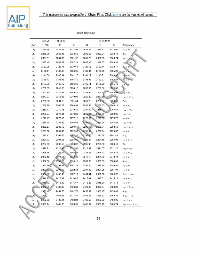
Table 2: (continued)

VMFCI H-RRBPM HI-RRBPM

Sym (11300) E A B C D Assignment

A2 2025.19 2024.46 2024.56 2024.29 2024.13 2024.00 ν5 + ν7

A1 2036.08 2033.45 2033.56 2032.63 2032.91 2032.78 2ν8

B2 2061.51 2061.39 2061.97 2061.79 2060.93 2060.74 ν15 + ν3

B1 2087.49 2086.87 2087.28 2087.05 2086.57 2086.38 ν12 + ν3

A2 2132.05 2129.74 2130.64 2129.78 2129.14 2128.77 ν8 + ν4

B2 2138.11 2136.36 2136.96 2136.34 2135.49 2135.21 ν8 + ν11

A1 2141.80 2140.94 2141.17 2141.17 2140.71 2140.60 ν5 + ν3

B1 2155.72 2153.95 2154.70 2153.95 2153.27 2152.89 ν8 + ν14

A1 2167.73 2166.12 2166.66 2166.11 2165.60 2165.40 ν8 + ν7

A1 2237.65 2240.00 2238.12 2235.85 2236.86 2236.66 2ν4

B1 2243.80 2245.63 2245.45 2243.34 2244.27 2243.99 ν4 + ν11

A2 2247.97 2248.85 2249.99 2250.02 2247.86 2247.45 ν15 + ν10

A1 2250.86 2264.16 2251.54 2250.26 2250.92 2250.81 2ν11

B2 2266.28 2267.58 2268.59 2267.68 2266.63 2266.13 ν7 + ν11

B2 2269.43 2270.18 2270.39 2269.52 2268.91 2268.67 ν14 + ν4

A2 2269.27 2270.34 2270.86 2269.81 2269.29 2268.95 ν14 + ν11

A2 2276.17 2277.09 2277.12 2276.32 2276.08 2275.77 ν7 + ν4

B2 2284.40 2285.89 2286.69 2285.50 2284.94 2284.58 ν15 + ν2

A1 2289.57 2289.13 2289.51 2289.46 2288.71 2288.50 ν12 + ν10

A2 2291.52 2291.40 2292.08 2291.43 2290.94 2290.67 ν3 + ν8

A1 2292.21 2303.56 2292.36 2291.58 2291.58 2291.41 2ν14

B1 2294.73 2304.48 2295.00 2294.04 2294.18 2294.02 ν7 + ν14

A1 2297.09 2306.59 2296.92 2295.90 2296.50 2296.40 2ν7

B1 2312.71 2312.47 2312.60 2312.37 2311.57 2311.26 ν12 + ν2

B1 2346.58 2346.02 2346.22 2346.06 2345.73 2345.49 ν5 + ν10

A1 2372.12 2371.51 2372.03 2372.17 2371.00 2370.74 ν5 + ν2

B2 2382.86 2390.19 2390.15 2383.58 2388.33 2388.00 3ν15

A1 2390.76 2391.54 2391.28 2391.00 2389.79 2389.51 ν3 + ν4

B1 2392.13 2391.88 2392.34 2391.99 2391.25 2391.01 ν3 + ν11

B1 2404.62 2407.45 2407.10 2404.41 2405.68 2405.27 2ν15 + ν12

B2 2416.22 2415.92 2416.42 2415.91 2415.31 2415.12 ν3 + ν14

A2 2416.72 2416.32 2416.67 2416.29 2415.90 2415.73 ν3 + ν7

B2 2430.50 2430.45 2430.83 2429.49 2429.54 2429.22 ν15 + 2ν12

B1 2460.42 2459.56 2462.70 2458.49 2460.17 2458.83 3ν12

A1 2467.01 2469.86 2474.80 2466.65 2469.33 2468.36 2ν15 + ν5

B2 2483.52 2482.81 2483.24 2482.63 2482.29 2482.05 ν10 + ν8

A2 2486.14 2485.88 2486.99 2485.04 2485.10 2484.74 ν15 + ν5 + ν12

31

Table 2: (continued)

VMFCI H-RRBPM HI-RRBPM

Sym (11300) E A B C D Assignment

A2 2510.34 2509.13 2510.00 2509.34 2508.45 2507.98 ν2 + ν8

A1 2512.47 2512.05 2516.28 2510.75 2515.86 2513.46 ν5 + 2ν12

A1 2538.02 2537.64 2538.14 2537.54 2537.53 2537.41 2ν3

B2 2548.58 2548.67 2550.79 2547.35 2548.93 2547.55 ν15 + 2ν5

B1 2569.28 2568.81 2569.65 2567.58 2568.29 2567.33 2ν5 + ν12

B1 2585.75 2585.35 2586.12 2585.36 2584.71 2584.32 ν10 + ν4

A1 2589.46 2589.29 2590.03 2589.20 2588.64 2588.24 ν10 + ν11

A2 2599.54 2602.32 2603.66 2603.79 2597.83 2597.09 2ν15 + ν8

A2 2601.69 2603.45 2605.07 2604.55 2600.79 2600.34 ν10 + ν14

B2 2603.53 2604.07 2605.83 2605.62 2602.61 2602.28 ν10 + ν7

A1 2615.39 2615.80 2618.38 2617.91 2614.57 2613.87 ν2 + ν4

B1 2618.85 2618.52 2619.63 2619.49 2617.66 2617.02 ν2 + ν11

A1 2621.28 2620.48 2622.40 2622.03 2618.87 2618.09 ν15 + ν12 + ν8

A1 2631.55 2630.68 2633.22 2629.95 2631.75 2630.88 3ν5

A2 2643.15 2643.17 2644.20 2643.53 2642.36 2641.75 ν2 + ν7

B2 2643.48 2643.50 2644.61 2644.14 2642.46 2641.91 ν2 + ν14

A2 2650.27 2647.84 2649.26 2649.22 2646.86 2646.24 2ν12 + ν8

B1 2680.29 2679.77 2682.25 2680.35 2678.79 2677.43 ν15 + ν5 + ν8

B1 2697.64 2700.08 2705.69 2701.16 2697.39 2696.02 2ν15 + ν11

B2 2704.29 2702.16 2706.41 2703.29 2702.57 2701.38 ν5 + ν12 + ν8

A1 2703.48 2705.90 2711.34 2705.45 2703.02 2701.69 2ν15 + ν4

A2 2715.21 2717.83 2723.95 2718.84 2714.95 2713.94 2ν15 + ν7

B2 2725.03 2725.32 2728.24 2726.45 2725.85 2723.68 ν15 + ν12 + ν11

A2 2731.66 2733.76 2736.98 2740.74 2732.82 2730.67 ν15 + ν12 + ν4

B2 2737.56 2740.10 2739.17 2742.98 2738.47 2736.72 2ν15 + ν14

B1 2737.96 2741.18 2742.30 2743.73 2738.73 2737.37 ν10 + ν3

A1 2747.23 2747.36 2750.19 2748.31 2745.92 2744.96 ν15 + ν12 + ν7

B1 2754.35 2754.49 2756.90 2755.04 2754.29 2752.71 ν15 + ν12 + ν14

A1 2760.02 2760.53 2764.07 2766.04 2759.13 2758.29 2ν12 + ν4

A2 2763.83 2762.10 2766.10 2768.07 2762.02 2761.35 2ν5 + ν8

B1 2763.28 2762.62 2768.07 2769.23 2762.23 2761.37 2ν12 + ν11

A1 2764.81 2767.68 2769.24 2771.66 2764.35 2763.88 ν2 + ν3

B2 2778.08 2776.81 2780.87 2777.59 2777.14 2775.59 2ν12 + ν14

A2 2786.85 2786.84 2790.83 2788.64 2786.73 2787.72 ν15 + ν5 + ν11

B2 2788.85 2788.26 2796.66 2789.21 2788.06 2788.41 ν15 + ν5 + ν4

A2 2792.07 2790.87 2797.51 2791.27 2791.19 2790.40 2ν12 + ν7

B1 2805.89 2805.94 2809.71 2806.50 2807.43 2809.98 ν15 + ν5 + ν7

32

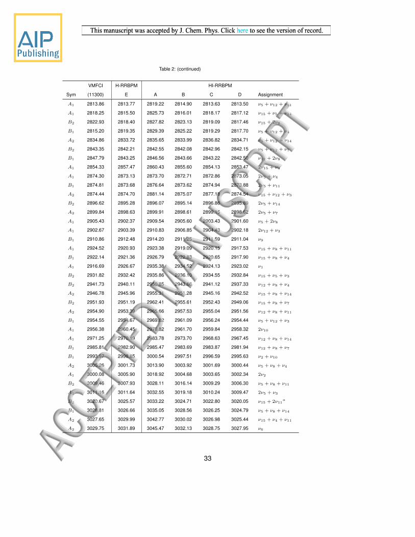
Table 2: (continued)

VMFCI H-RRBPM HI-RRBPM

Sym (11300) E A B C D Assignment

A1 2813.86 2813.77 2819.22 2814.90 2813.63 2813.50 ν5 + ν12 + ν11

A1 2818.25 2815.50 2825.73 2816.01 2818.17 2817.12 ν15 + ν5 + ν14

B2 2822.93 2818.40 2827.82 2823.13 2819.09 2817.46 ν15 + 2ν8

B1 2815.20 2819.35 2829.39 2825.22 2819.29 2817.70 ν5 + ν12 + ν4

A2 2834.86 2833.72 2835.65 2833.99 2836.82 2834.71 ν5 + ν12 + ν14

B2 2843.35 2842.21 2842.55 2842.08 2842.96 2842.15 ν5 + ν12 + ν7

B1 2847.79 2843.25 2846.56 2843.66 2843.22 2842.50 ν12 + 2ν8

A1 2854.33 2857.47 2860.43 2855.60 2854.13 2853.47 2ν15 + ν3

A1 2874.30 2873.13 2873.70 2872.71 2872.86 2873.05 2ν5 + ν4

B1 2874.81 2873.68 2876.64 2873.62 2874.94 2873.88 2ν5 + ν11

A2 2874.44 2874.70 2881.14 2875.07 2877.18 2874.54 ν15 + ν12 + ν3

B2 2896.62 2895.28 2896.07 2895.14 2896.86 2895.89 2ν5 + ν14

A2 2899.84 2898.63 2899.91 2898.61 2899.15 2898.62 2ν5 + ν7

A1 2905.43 2902.37 2909.54 2905.60 2903.43 2901.60 ν5 + 2ν8

A1 2902.67 2903.39 2910.83 2906.85 2904.43 2902.18 2ν12 + ν3

B1 2910.86 2912.48 2914.20 2911.25 2911.59 2911.04 ν9

A1 2924.52 2920.93 2923.38 2919.09 2920.15 2917.53 ν15 + ν8 + ν11

B1 2922.14 2921.36 2926.79 2922.83 2920.65 2917.90 ν15 + ν8 + ν4

A1 2916.69 2926.67 2935.38 2934.52 2924.13 2923.02 ν1

B2 2931.82 2932.42 2935.86 2936.10 2934.55 2932.84 ν15 + ν5 + ν3

B2 2941.73 2940.11 2950.85 2943.66 2941.12 2937.33 ν12 + ν8 + ν4

A2 2946.78 2945.96 2955.31 2951.28 2945.16 2942.52 ν15 + ν8 + ν14

B2 2951.93 2951.19 2962.41 2955.61 2952.43 2949.06 ν15 + ν8 + ν7

A2 2954.90 2953.39 2965.66 2957.53 2955.04 2951.56 ν12 + ν8 + ν11

B1 2954.55 2954.67 2969.82 2961.09 2956.24 2954.44 ν5 + ν12 + ν3

A1 2956.38 2960.45 2978.82 2961.70 2959.84 2958.32 2ν10

A1 2971.25 2970.19 2983.78 2973.70 2968.63 2967.45 ν12 + ν8 + ν14

B1 2985.81 2982.90 2985.47 2983.69 2983.87 2981.94 ν12 + ν8 + ν7

B1 2993.97 2998.85 3000.54 2997.51 2996.59 2995.63 ν2 + ν10

A2 3005.26 3001.73 3013.90 3003.92 3001.69 3000.44 ν5 + ν8 + ν4

A1 3000.08 3005.90 3018.92 3004.68 3003.65 3002.34 2ν2

B2 3009.46 3007.93 3028.11 3016.14 3009.29 3006.30 ν5 + ν8 + ν11

A1 3011.16 3011.64 3032.55 3019.18 3010.24 3009.47 2ν5 + ν3

B2 3020.67 3025.57 3033.22 3024.71 3022.80 3020.05 ν15 + 2ν11a

B1 3028.81 3026.66 3035.05 3028.56 3026.25 3024.79 ν5 + ν8 + ν14

A2 3027.65 3029.99 3042.77 3030.02 3026.98 3025.44 ν15 + ν4 + ν11

A2 3029.75 3031.89 3045.47 3032.13 3028.75 3027.95 ν6

33

Table 2: (continued)

VMFCI H-RRBPM HI-RRBPM

Sym (11300) E A B C D Assignment

B2 3035.82 3037.35 3047.57 3035.91 3037.58 3033.86 ν15 + 2ν4a

A1 3039.04 3041.79 3049.07 3039.54 3039.05 3035.70 ν5 + ν8 + ν7

B1 3038.05 3043.43 3052.84 3046.25 3040.13 3038.36 2ν15 + ν10

B2 3041.99 3046.18 3056.30 3046.47 3041.32 3040.21 ν13

B1 3049.21 3052.14 3059.30 3048.02 3049.66 3048.42 ν12 + 2ν11b

A1 3047.88 3054.71 3061.21 3050.41 3050.54 3048.70 ν15 + ν7 + ν11

A2 3055.15 3054.90 3069.00 3055.09 3052.21 3048.87 3ν8

B1 3055.92 3059.55 3070.07 3059.59 3058.91 3057.21 ν15 + ν14 + ν11

A1 3057.68 3061.32 3071.45 3061.04 3061.71 3060.39 ν12 + ν4 + ν11

A1 3061.06 3065.37 3077.15 3069.47 3066.80 3061.69 ν15 + ν14 + ν4

B1 3064.98 3069.01 3079.92 3074.17 3069.46 3066.08 ν15 + ν7 + ν4

B2 3066.76 3069.52 3081.24 3076.92 3071.96 3066.94 ν15 + ν12 + ν10

B1 3069.49 3079.01 3085.87 3077.25 3073.61 3069.95 ν12 + 2ν4b

A1 3068.03 3079.80 3087.90 3079.26 3075.33 3071.18 2ν15 + ν2

B2 3073.86 3082.54 3091.53 3084.88 3075.83 3072.99 ν15 + 2ν14c

A2 3073.86 3084.47 3093.22 3086.12 3079.16 3074.73 ν12 + ν14 + ν4d

B1 3078.94 3084.85 3096.10 3090.57 3084.71 3079.51 ν15 + ν3 + ν8

B2 3084.92 3087.10 3100.08 3090.96 3087.53 3084.54 ν12 + ν14 + ν11

A2 3084.02 3089.09 3101.81 3094.57 3088.76 3085.65 ν15 + ν12 + ν2

A2 3087.97 3095.81 3109.45 3096.20 3091.32 3088.11 ν15 + ν7 + ν14

B2 3089.06 3099.08 3110.45 3098.78 3095.50 3088.58 ν15 + 2ν7c

B2 3096.23 3100.35 3114.11 3102.13 3103.41 3098.61 ν12 + ν7 + ν4

A2 3102.56 3105.14 3120.94 3104.78 3105.01 3102.95 ν12 + ν7 + ν11

B2 3104.44 3105.55 3125.34 3106.60 3107.51 3103.16 ν12 + ν3 + ν8

B1 3105.97 3108.65 3127.67 3106.91 3110.65 3104.30 ν12 + 2ν14

B1 3109.55 3114.93 3128.20 3110.84 3111.75 3109.15 2ν12 + ν10

A1 3116.35 3116.00 3129.81 3114.59 3115.43 3112.80 ν5 + 2ν11e

A1 3112.92 3120.45 3131.77 3115.53 3120.70 3115.58 ν12 + ν7 + ν14

B1 3118.38 3122.67 3132.70 3120.44 3122.67 3119.83 ν5 + ν4 + ν11

B1 3122.34 3127.29 3136.78 3123.52 3124.84 3121.56 ν12 + 2ν7

A1 3127.59 3129.90 3139.27 3124.07 3131.31 3125.67 ν5 + 2ν4e

A2 3126.44 3130.56 3140.66 3130.28 3132.82 3125.96 ν15 + ν5 + ν10

A1 3129.22 3139.09 3151.45 3132.42 3136.56 3127.61 2ν12 + ν2

A1 3146.79 3139.62 3152.82 3139.95 3142.00 3134.62 2ν8 + ν4

B2 3143.48 3142.25 3155.87 3143.02 3143.03 3141.97 ν5 + ν7 + ν11

B2 3146.04 3143.82 3156.69 3145.39 3145.07 3142.77 ν5 + ν14 + ν4

A2 3143.09 3145.01 3162.41 3147.67 3153.11 3143.98 ν5 + ν14 + ν11

34

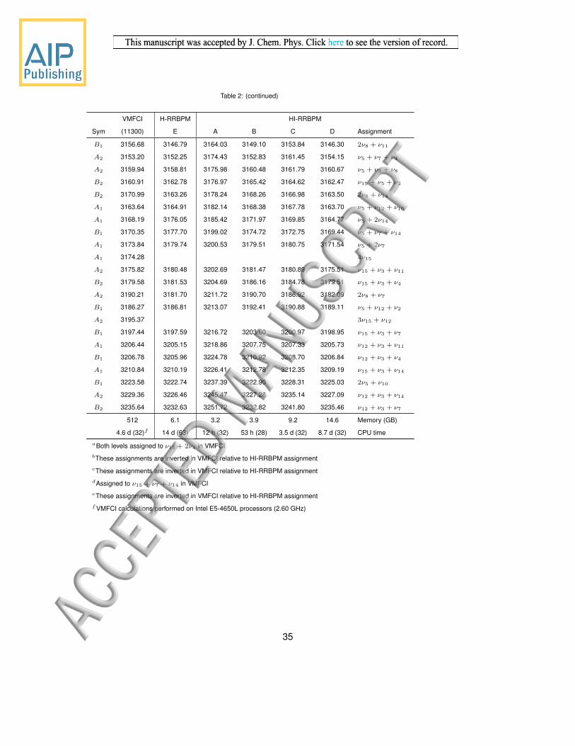
Table 2: (continued)

VMFCI H-RRBPM HI-RRBPM

Sym (11300) E A B C D Assignment

B1 3156.68 3146.79 3164.03 3149.10 3153.84 3146.30 2ν8 + ν11

A2 3153.20 3152.25 3174.43 3152.83 3161.45 3154.15 ν5 + ν7 + ν4

A2 3159.94 3158.81 3175.98 3160.48 3161.79 3160.67 ν5 + ν3 + ν8

B2 3160.91 3162.78 3176.97 3165.42 3164.62 3162.47 ν15 + ν5 + ν2

B2 3170.99 3163.26 3178.24 3168.26 3166.98 3163.50 2ν8 + ν14

A1 3163.64 3164.91 3182.14 3168.38 3167.78 3163.70 ν5 + ν12 + ν10

A1 3168.19 3176.05 3185.42 3171.97 3169.85 3164.77 ν5 + 2ν14

B1 3170.35 3177.70 3199.02 3174.72 3172.75 3169.44 ν5 + ν7 + ν14

A1 3173.84 3179.74 3200.53 3179.51 3180.75 3171.54 ν5 + 2ν7

A1 3174.28 4ν15

A2 3175.82 3180.48 3202.69 3181.47 3180.89 3175.51 ν15 + ν3 + ν11

B2 3179.58 3181.53 3204.69 3186.16 3184.78 3179.51 ν15 + ν3 + ν4

A2 3190.21 3181.70 3211.72 3190.70 3186.92 3182.09 2ν8 + ν7

B1 3186.27 3186.81 3213.07 3192.41 3190.88 3189.11 ν5 + ν12 + ν2

A2 3195.37 3ν15 + ν12

B1 3197.44 3197.59 3216.72 3203.60 3200.97 3198.95 ν15 + ν3 + ν7

A1 3206.44 3205.15 3218.86 3207.75 3207.33 3205.73 ν12 + ν3 + ν11

B1 3206.78 3205.96 3224.78 3210.92 3208.70 3206.84 ν12 + ν3 + ν4

A1 3210.84 3210.19 3226.41 3212.78 3212.35 3209.19 ν15 + ν3 + ν14

B1 3223.58 3222.74 3237.39 3222.90 3228.31 3225.03 2ν5 + ν10

A2 3229.36 3226.46 3245.47 3227.28 3235.14 3227.09 ν12 + ν3 + ν14

B2 3235.64 3232.63 3251.72 3232.82 3241.80 3235.46 ν12 + ν3 + ν7

512 6.1 3.2 3.9 9.2 14.6 Memory (GB)

4.6 d (32)f 14 d (63) 12 h (32) 53 h (28) 3.5 d (32) 8.7 d (32) CPU time

aBoth levels assigned to ν15 + 2ν4 in VMFCIbThese assignments are inverted in VMFCI relative to HI-RRBPM assignmentcThese assignments are inverted in VMFCI relative to HI-RRBPM assignmentdAssigned to ν15 + ν7 + ν14 in VMFCIeThese assignments are inverted in VMFCI relative to HI-RRBPM assignmentfVMFCI calculations performed on Intel E5-4650L processors (2.60 GHz)

35

Table 3: Parameters for HI-RRBPM calculations on cyclopentadiene.Parameter A B C D E F

Rψ 60 100 150 240 300 360NCPU 32a 32b 32b 64b 32a 32a

NeALS;ψ 1 1 1 1 1 1Ncyc 20 20 20 20 20c 10d

Nsweep 10 10 10 10 10 10Memory (GB) 9.7 15.9 24.6 83.9 56.9 72.4

Wall time 43.0 h 32.2 d 61.1 d 50.2 d 31.3 d 22.8 daIntel Xeon E5-2670 0 processors running at 2.6 GHzbAMD Opteron 6386 SE processors running at 2.8 GHzcContinuation of ’A’ calculation with larger rankdContinuation of ’E’ calculation with larger rankeFor rank reductions in Gram-Schmidt, vector updates, and H(F) = FTHF steps.

36

Table 4: Fundamental vibrational levels (cm−1) computed for cyclopentadiene using HI-

RRBPM, in comparison to VPT2 values.

Sym VPT2 HI-RRBPM Assignment

A B C D E F

A1 19911.13 19907.80 19906.52 19904.74 19904.28 19903.98 ZPE

B1 342 318.55 317.19 315.50 314.00 313.95 313.64 ν19

A2 516 509.48 508.06 507.48 506.50 506.41 506.25 ν14

B1 666 654.48 653.09 650.44 648.21 647.87 647.58 ν18

A2 701 688.11 686.26 684.91 684.21 684.00 683.81 ν13

B2 802 802.47 800.48 800.02 798.94 798.61 798.32 ν27

A1 802 805.68 802.35 802.07 800.72 800.59 800.38 ν10

B1 888 877.30 874.93 872.79 870.78 870.41 870.07 ν17

A1 906 909.50 907.21 907.12 905.87 905.79 905.43 ν9

B1 933 924.11 919.85 922.24 918.03 918.15 917.59 ν16

A2 932 925.85 921.89 921.74 918.31 918.88 919.33 ν12

B2 949 948.21 945.21 944.12 943.35 942.84 942.51 ν26

A1 991 1005.74 996.10 994.20 992.81 992.00 991.61 ν8

A2 1088 1084.87 1083.21 1080.38 1078.48 1078.19 1077.84 ν11

B2 1093 1091.48 1089.46 1088.58 1086.18 1085.89 1085.41 ν25

A1 1112 1112.64 1110.12 1108.80 1106.84 1106.88 1106.48 ν7

B2 1221 1227.81 1221.25 1219.36 1214.97 1213.94 1213.06 ν24

B2 1285 1288.22 1283.87 1282.35 1280.77 1283.69 1283.08 ν23

A1 1361 1363.22 1355.17 1350.45 1347.37 1346.65 1345.91 ν6

A1 1371 1375.40 1370.90 1368.86 1366.29 1366.00 1365.49 ν5

A1 1501 1523.47 1521.22 1503.45 1499.54 1499.19 1498.45 ν4

B2 1592 1659.00 1615.76 1601.14 1592.35 1591.29 1590.09 ν22

37

Figure 1: Ethylene oxide

38

q15 q8q2 q3q10q5 q12 q1 q9q6 q13 q740 30 2030 30 20 20 20 3020 20 20

q4q14 q112020 20

20 12 1119 19 11 11 14 1411 8 10 1010 10

84 70 7070

200

20 55 55 55 55 55 55 55

q15 q8q2 q3q10q5 q12 q1 q9q6 q13 q740 30 2030 30 20 20 20 3020 20 20

q4q14 q112020 20

20 12 1119 19 11 11 14 1411 8 10 1010 10

120 111 126126

200

20 361 121 132 112 154 100 100

20 78 76 77 68 74 79 79

a)

b)

Figure 2: Trees used in calculations on ethylene oxide: a) medium tree, and b) large tree. Numbersappearing at vertices are basis sizes; placement of the primitive coordinates in the leaf nodes isshown at the bottom of the tree.

39

Figure 3: Cyclopentadiene

40

q1 q11q4 q6q5q20 q2 q15 q22q21 q3 q24

99 99 9999 99 99 99 99 9999 99 99q7q23 q25

9999 99

20 20 2020 20 20 20 20 2020 20 20 2020 20

210 210 220

192

q27q14 q17q19q13 q18q12 q16 q10

99 9999 99 99 9999 99 99q9q26 q8

9999 99

30 3030 30 30 3030 30 30 3030 30

166 220165

20 30 30400 400 400 400 400 400 400 900 900 900 900 900

210 101

20 30 30105 105 101 105 105 108 105 108103 116 105 105

210 105121 165 166 105 120

C−H stretch C−C stretch C−H rocking out-of-plane rocking ring breathe

Figure 4: Tree used in calculations on cyclopentadiene. Numbers appearing at vertices are basissizes; placement of the primitive coordinates in the leaf nodes is shown at the bottom of the tree.

41

http://dx.doi.org/10.1063/1.4983695

q 15

q 8q 2

q 3q 10

q 5q 12

q 1q 9

q 6q 13

q 740

3020

3030

2020

2030

2020

20q 4

q 14

q 11

2020

20

2012

1119

1911

1114

1411

810

1010

10

8470

7070

200

2055

5555

5555

5555

q 15

q 8q 2

q 3q 10

q 5q 12

q 1q 9

q 6q 13

q 740

3020

3030

2020

2030

2020

20q 4

q 14

q 11

2020

20

2012

1119

1911

1114

1411

810

1010

10

120

111

126

126

200

20361

121

132

112

154

100

100

2078

7677

6874

7979

a) b)

http://dx.doi.org/10.1063/1.4983695

q 1q 1

1q 4

q 6q 5

q 20

q 2q 1

5q 2

2q 2

1q 3

q 24

9999

9999

9999

9999

9999

9999

q 7q 2

3q 2

5

9999

99

2020

2020

2020

2020

2020

2020

2020

20

210

210

220

192

q 27

q 14

q 17

q 19

q 13

q 18

q 12

q 16

q 10

9999

9999

9999

9999

99q 9

q 26

q 899

9999

3030

3030

3030

3030

3030

3030

166

220

165

2030

30400

400

400

400

400

400

400

900

900

900

900

900

210

101

2030

30105

105

101

105

105

108

105

108

103

116

105

105

210

105

121

165

166

105

120

C−H

stre

tch

C−C

stre

tch

C−H

rock

ing

out-o

f-pla

nero

ckin

grin

g br

eath

e