F M An Introduction to FREQUENCY MODULATION By JOHN F. RIDER AUTHOR OF Perpetual Trouble Shooter's Manuals and other books for the Radio Service Industry JOHN F. RIDER PUBLISHER, INC. 404 FOURTH AVENUE NEW YORK CITY
Transcript
F M An Introduction to
FREQUENCY MODULATION
By
JOHN F. RIDER AUTHOR OF
Perpetual Trouble Shooter's Manuals and other books for the Radio Service Industry
JOHN F. RIDER PUBLISHER, INC.
404 FOURTH AVENUE NEW YORK CITY
Copyright, 1940, by JOHN F. RIDER
All rights reserved including that of translation into the Scandinavian and other foreign languages
Printed in the 'United States of America
Dedicated to the
RADIO SERVICE MAN
to whom radio developments are a boon as well as a problem
INTRODUCTION
UNTIL recently, all commercial broadcast stations, ir- respective of their operating frequencies, employed what is known as amplitude -modulated waves for
the transmission of their programs; and as is to be expected all the receivers intended for the reception of these pro- grams were designed to derive the proper intelligence from such amplitude -modulated waves. The past few months, however, have witnessed a great deal of agitation about a new form of transmission, known as frequency modulation -the brain child of Major E. H. Armstrong. In fact quite a few broadcast stations have already installed secondary transmitters operating upon experimental licenses and are transmitting such frequency -modulated waves. The num- ber of these stations is growing daily and their locations are beginning to spread across the breadth of the nation. In order to provide reception of these programs, some of the larger commercial receiver manufacturers are in production of what are known as frequency -modulation receivers and substantial quantities have been sold to the public.
As all signs point to an extremely rapid growth of this form of transmission and the widespread use of such re- ceivers, the subject in general is becoming of interest to the radio servicing industry. To meet the immediate demand for information concerning the general theory underlying the operation of such receivers and the problems of servic- ing, this book, which is intended as an introduction to the subject of Frequency Modulation, was written.
The subject is new and all of its ramifications and prob- lems are not known as yet, hence this volume of compara- tively few pages is not intended as a complete exposition of the subject. Its primary purpose is to place in the hands of the servicing industry such pertinent information as will furnish a general outline of frequency modulation: the
iv
INTRODUCTION
manner in which it differs from amplitude modulation, and details associated with f -m receiver servicing problems.
The subject of frequency modulation involves some con- tradictions of existing practices and in general introduces new thoughts in connection with the operation of radio communication systems, transmitters and receivers alike. This book discusses some of these new ideas from an ele- mentary viewpoint: with sufficient detail to enable a serv- ice man to speak intelligently when asked questions, which no doubt will be numerous in the near future, and to be able to service a receiver brought into his shop.
The critical engineer who reads these pages will find much detail missing: the mathematical solutions, the elab- orations and variations of certain theoretical principles which are presented as results accomplished. In fact he might even find a departure from absolute preciseness, wherever it is necessary in order to present a point in the most comprehensive manner. We must bear in mind that the many thousands of men who have done such creditable work maintaining the public's tens of millions of radio re- ceivers, and for whom this book is intended, are not engi- neers.
Being guided by what has happened in the past twenty years the attention of the servicing industry has been fo- cused upon the receiver rather than the transmitter. Such is the case in this book. The discussions of the means of developing frequency -modulated waves are brief, with suf- ficient detail, we hope, to give the reader a general but clear idea of what is happening. Definite, specific standards are not given because from all information available at the time of this writing, standards have not yet reached con- crete form.
The discussion of receivers embraces, of course, the gen- eral differences between f -m and a -m systems and where specific references are given, they are limited by the fact that at the time of this writing but a few brands of re- ceivers are available. No doubt by the time this book is off the press, additional commercial receiver manufactur-
vi INTRODUCTION
ers, who have stated their intention to produce f -m receiv- ers, will have made them available to the public.
In connection with the details given concerning the re- ceiver we might say again that the critical observer will find certain technical details missing. This is deliberate in that while the inclusion of the information would advance the reader, its omission in no way impairs the utility of the book, but does obviate the necessity for the presentation of certain mathematical details which are not pertinent to the servicing problem. For the man who is interested in delv- ing deeper into the subject of frequency modulation, a bib- liography of texts relating thereto is included and we are certain anyone interested will find in these reference texts far more data than we can furnish between the covers of this book.
The material contained in the servicing chapter is, as you can see, the result of actual experimental work and also includes data gathered from whatever available sources exist. The receivers being new and transmission still limi- ted, much data that might be of value are not yet avail- able. Only years of field experience embracing all forms of difficulties can round out the servicing picture. How- ever, the receivers are out in the field; a certain amount of practical servicing experience has been had; an appreciable amount of experimental work has been carried on, so that a fairly comprehensive picture of servicing problems is pos- sible.
You will note references to signal tracing in the servicing section. Signal tracing as a means of locating defects is just as applicable to f -m receivers as it has proved itself to a -m receivers, for after all is said and done, the f -m signal is just a signal. However we have also included other forms of servicing technique; so as to embrace all types of servicing apparatus.
We trust that this introduction to frequency modulation will fill the gap until bigger and better books are available.
JOHN F. RIDER. March, 1940.
TABLE OF CONTENTS
CHAPTER I. FREQUENCY MODULATION -1. Amplitude Modulation -1. Frequency Modulation -3. F -M Band Width -5. Percentage of Modulation -7. The F -M Receiver -8. Summary of F -M Waves -10.
CHAPTER II. WHAT HAPPENS AT THE TRANSMITTER - 11. Simplest Frequency Modulator -12. Frequency Modula- tion by Amplification -20. Increasing Shift by Frequency Doubling -23. The Armstrong System -25. Phase Shift and Frequency Shift -27. Effect of Audio Frequency Upon a
Phase -Modulated Wave -34. Deviation Ratio -36.
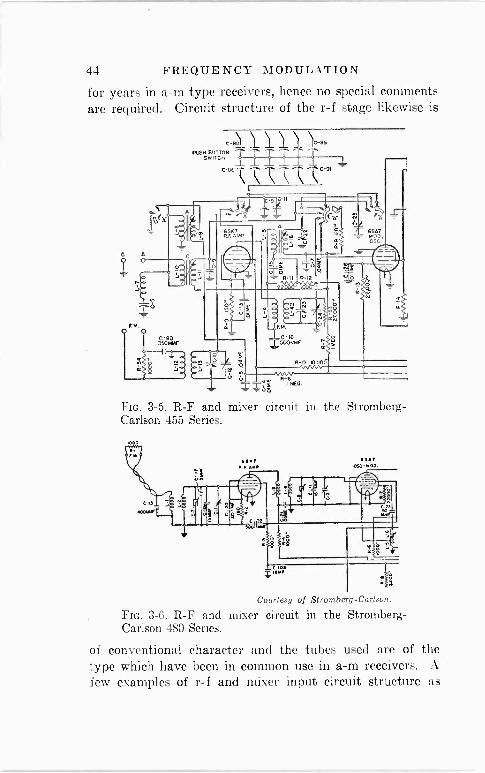
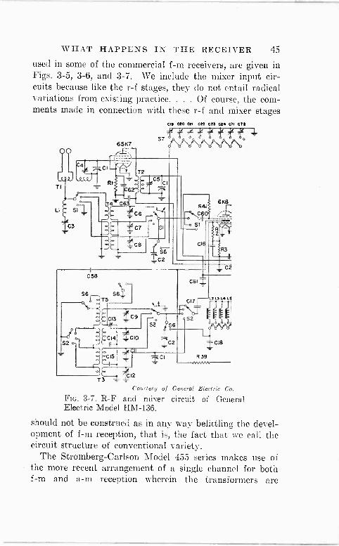
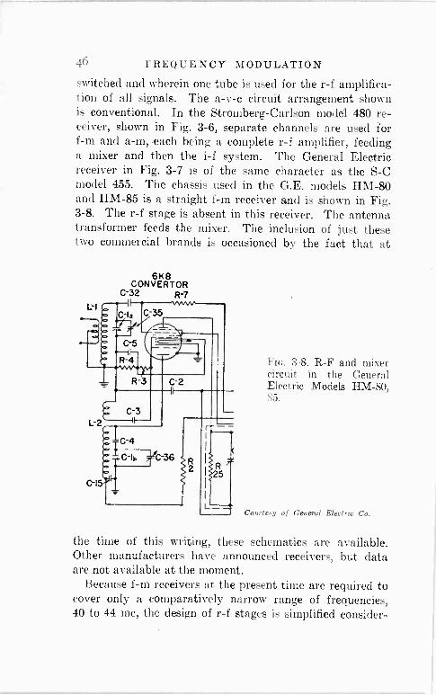
CHAPTER III. WHAT HAPPENS IN THE RECEIVER -37. Function of R -F Tuned Circuits in F -M Receivers -38. Car- rier Frequency Amplification -39. Typical R -F Circuits 43.
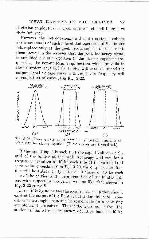
The Mixer and Oscillator Systems -47. The I -F System -4S. Amplification in I -F Stages -50. The Limiter Stage -53. Varying Sensitivity of Limiter -59. Signal Input vs Signal Output at the Limiter -61. Selectivity Characteristics of I -F Amplifier -64. Types of Limiter Circuits -69. AVC in F -M Receivers -70. The Discriminator -71. Center -Tapped Sec- ondary Type of Discriminator -78. Off Resonance Condi- tions -81. Linearity of Discriminator -82.
CHAPTER IV. THE TRANSMISSION OF F -M SIGNALS -85. How Are F -M Signals Propagated -86. Range of Signals Above 30 MC -89. Beyond the Horizon Range -91. Service Areas of F -M Stations -92.
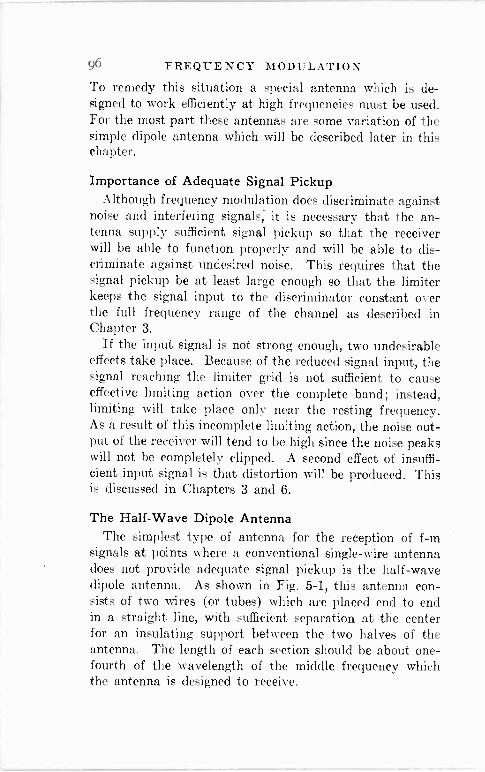
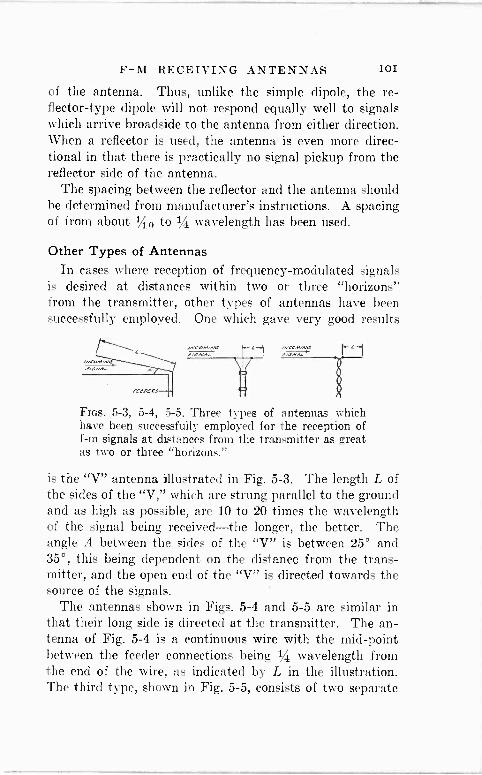
CHAPTER V. F -M RECEIVING ANTENNAS -95. Importance of Adequate Signal Pickup -96. The Half -Wave Dipole An- tenna -96. Length of Dipole -98. Polarization -99. Dipole with Reflector -100. Other Types of Antennas -101.
CHAPTER VI. SERVICING F -M RECEIVERS -103. Oscillators or Signal Sources for Alignment -103. Service Equipment - 106. Interference --107. Regeneration -109. Noise -111.
vii
Vnl CONTENTS Signal Tracing -113. The I -F System -117. Shift of Peak in Limiter Grid Circuit -117. Low Impedance Across Oscil- lator Output -119. Signal At Limiter Plate -119. The Dis- criminator -121. Methods of Alignment -122. Visual Method of Alignment -123. D -C Voltmeter Indication in Visual Align- ment -127. Use of Marker Frequency -129. Fixed -Fre- quency Alignment -131. The Oscillator -131. The R -F and Mixer -132. Automatic Volume Control -132. The Audio System -134.
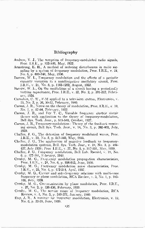
BIBLIOGRAPHY -135.
Chapter I
FREQUENCY MODULATION
WHAT is frequency modulation? ..While the
question is simple, the answer is a bit more com- plex, although it is not difficult of comprehension.
Judging from the comments heard, many people believe it to be a new form of transmission. Such is not the case. In reality it is a new make-up or structure of the trans- mitted signal. If we express it differently, it is a new way of combining the intelligence to be transmitted via radio with the basic radio signal. The net result is a radio signal with characteristics different from that which has been used heretofore.
Amplitude Modulation Amplitude modulation has been the usual form of com-
bining the intelligence to be transmitted with the actual radio signal and it has been accepted practice to describe this transmitted wave in terms of the type of modulation. By amplitude modulation is meant the combination of the modulating signal, which is the speech, music or the infor- mation to be conveyed, in such a manner that the modu- lating signal alternately increases and decreases the amplitude of the radio signal; this variation taking place at a rate determined by the frequency of the audio signal. The extent of this change in carrier level depends upon the relative magnitudes of the audio and the carrier signals at the instant they are combined and also upon the design of the system with respect to the percentage of modulation. Neglecting the percentage of modulation at the moment, let it be said that the stronger the audio signal combined with
2 FREQUENCY MODULATION
the carrier, the greater is the change in the amplitude of
the carrier. This is of particular importance with respect to what is to follow.
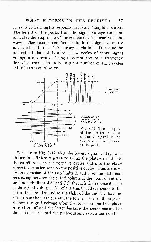
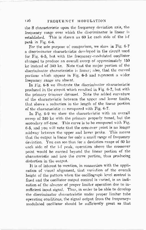
Naturally a definite relationship always existed between the audio signal level and the carrier signal level, both as to percentage of modulation and distortion. If the audio voltage was excessive with respect to the carrier level, then over -modulation would occur with resultant distortion. On the other hand if the audio level was less than a certain amount, then the desired percentage of modulation would not be obtained. All of these conditions are shown in Figs. 1-1, 1-2, 1-3, 1-4 and 1-5, wherein are illustrated the car -
III III II 1 IIII
III 1111111111111 F/G. 1- 1
FIG. l-4
F G. /-2
FIG. /-S
F/G. 1-3
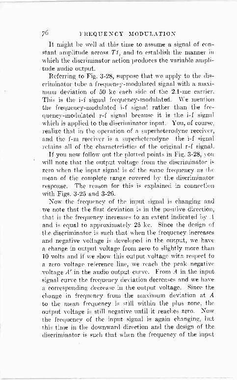
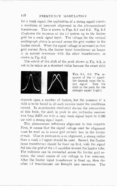
FIGS. 1-1 to 1-5. An amplitude -modu- lated carrier with various percentages of modulation rang- ing from zero mod- ulation to overmod- ulation. Fig. 1-2 shows the modulat- ing voltage.
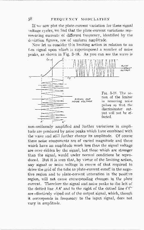
rier without modulation, the audio (modulating) signal, the equivalent of 50 -percent modulation, the equivalent of 100 -
percent modulation, and over -modulation. Certain very significant details are associated with such
amplitude -modulated waves. In the first place the wave when modulated is not of constant amplitude; in fact it is
anything but constant, varying definitely with the ampli- tude of the audio signal. The second detail is that the composition of such an amplitude -modulated wave consists of the carrier frequency and a series of other frequencies representing various plus and minus combinations of the carrier and the modulating frequencies. These combinations
FREQUENCY MODULATION 3
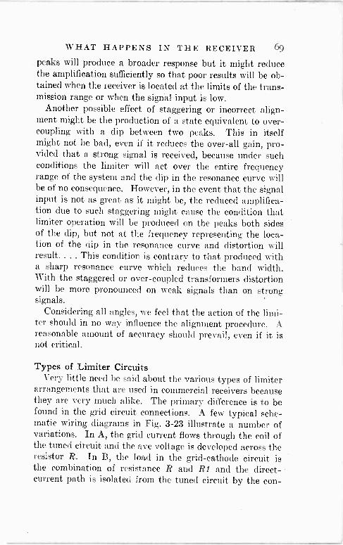
represent the sidebands of the carrier. The higher the fre- quency of the audio voltage used to modulate the carrier, the greater is the extent of the sidebands. The third' detail is that while we recognize the existence of sidebands, the significance of the frequency of the audio voltage is in terms of how rapidly in a unit of time, say one second, the ampli- tude (not the frequency) of the carrier is increased and de- creased in accordance with the strength of the audio signal.
Such amplitude -modulated form of transmission has been used for a long time, but certain disadvantages were con- tinually apparent. One of these was the natural and man- made static problem. This was brought about by the effect of such disturbances upon the received signal. Investiga- tion disclosed that when such electrical disturbances com- bined with the electrical wave in the receiver, the result was a change in amplitude of the carrier, just as if this dis- turbance was an audio voltage. And with the design of the conventional receiver being of such type that it re- sponded primarily to variations in amplitude of the carrier, the elimination of noise became an extremely difficult prob- lem.... In fact under certain conditions when the noise - to -signal ratio was high, any attempt to remove or even decrease the noise, removed or decreased the signal as well. At times, the noise reached such proportions that actual operation of the communication or broadcasting system was impossible. The search to alleviate the situation embraced many operations, such as selecting higher carrier frequen- cies, the development of noise -reducing circuits, municipal ordinances for filtering of noise -producing apparatus, the use of higher power at the transmitters, etc., but the solu- tion was not complete. Something else was needed... .
That something else seems to be frequency modulation.
Frequency Modulation How does frequency modulation differ from amplitude
modulation? It differs in many respects. ... One of the most important is that in contrast to the varying amplitude of the amplitude -modulated carrier, the frequency-modu-
4 FREQUENCY MODULATION
lated carrier remains constant in amplitude. The second is that the modulation applied to the carrier causes changes in frequency of the radiated signal. In contrast to the con- ditions existing in a -m form of signal transmission, the level of the audio modulation determines the shift or deviation in frequency in the f -m system. The stronger the audio signal, the greater is the change in frequency. As to the frequency of the audio -modulating signal, this determines the number of times per second that the change or deviation in frequency of the carrier takes place. The higher the frequency of the audio or modulating voltage in the trans- mitter, the greater the number of times per second that the carrier frequency changes between the limits determined by the amplitude or strength of the audio signal.
To illustrate the frequency -modulated wave upon the same plane as that used for the amplitude -modulated wave -that is, a two-dimensional picture-we offer Fig. 1-6, wherein the height of the vertical lines indicates that the carrier remains constant in level, and the variation in sep- aration of the lines indicates that the frequency changes in accordance with the audio amplitude. This becomes evident if you correlate Figs. 1-6 and 1-7.
Now in regards to the relation between noise and the frequency -modulated form of transmission, two conditions contribute to virtual freedom from this type of interference. One of these conditions is that the entire system is predi- cated upon a changing frequency of the carrier and noise does not materially affect the frequency. As to the change in amplitude of the wave because of noise, one function of a portion of the f -m receiver is to maintain a constant level of the carrier and to eliminate any changes in the carrier amplitude. Hence ,if noise tends to change the carrier am- plitude, these amplitude variations are removed and so, in effect, the noise is removed as well. The limiter stage in the receiver performs this function. The discriminator in the f -m receiver translates varying frequency signals into audio signals and since noise does not materially change the
FREQUENCY MODULATION 5
frequency, the discriminator contributes its share towards noise reduction.
Whereas in an amplitude -modulation receiver, instanta- neous changes in carrier amplitude are taking place through- out the receiver until the audio component is separated from
I I IIIII I I III IIIIII I I I
Iil I Y !IA!? !!!\ III T/ME
Ftcs. 1-6, 1-7. A frequency -modulated signal in which the frequency of the signal varies in accord- ance with the level of the modulating audio voltage. At points where the audio voltage is positive, the frequency is high, while at points where the audio voltage is negative, the frequency is low.
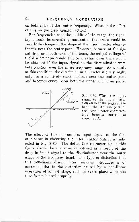
the carrier, in the frequency -modulation receiver the carrier amplitude is held constant and only at that point where the audio- and radio -frequency signals are separated, do am- plitude variations take place-and even here, the carrier frequency variations are translated into audio amplitude variations. Thus, in the frequency -modulation form of transmission, we start out and end with only audio - frequency amplitude variations. In all the other portions of the transmitter and the receiver, r -f signals are of con- stant amplitude but changing frequency.
F -M Band Width It is only natural that having read statements concerning
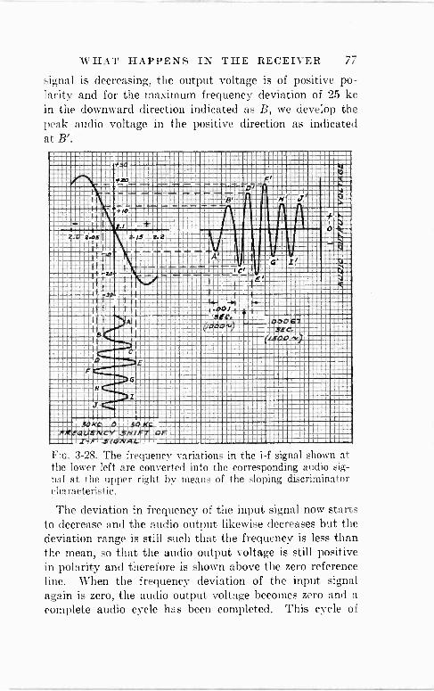
changes in frequency of the carrier, you might be interested in more specific illustrations of just what is meant by these
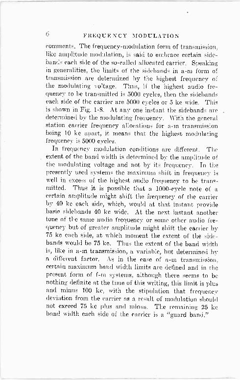
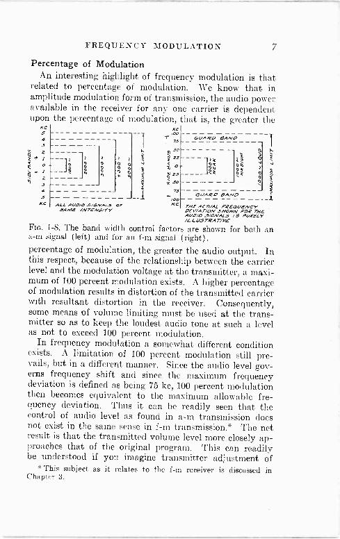
6 FREQUENCY MODULATION comments. The frequency -modulation form of transmission, like amplitude modulation, is said to embrace certain side - bands each side of the so-called allocated carrier. Speaking in generalities, the limits of the sidebands in a -m form of transmission are determined by the highest frequency of the modulating voltage. Thus, if the highest audio fre- quency to be transmitted is 5000 cycles, then the sidebands each side of the carrier are 5000 cycles or 5 kc wide. This is shown in Fig. 1-8. At any one instant the sidebands are determined by the modulating frequency. With the general station carrier frequency allocations for a -m transmission being 10 kc apart, it means that the highest modulating frequency is 5000 cycles.
In frequency modulation conditions are different. The extent of the band width is determined by the amplitude of the modulating voltage and not by its frequency. In the presently used systems the maximum shift in frequency is well in excess of the highest audio frequency to be trans- mitted. Thus it is possible that a 1000 -cycle note of a certain amplitude might shift the frequency of the carrier by 40 kc each side, which, would at that instant provide basic sidebands 40 kc wide. At the next instant another tone of the same audio frequency or some other audio fre- quency but of greater amplitude might shift the carrier by 75 kc each side, at which moment the extent of the side - bands would be 75 kc. Thus the extent of the band width is, like in a -m transmission, a variable, but determined by a different factor. As in the case of a -m transmission, certain maximum band width limits are defined and in the present form of f -m systems, although there seems to be nothing definite at the time of this writing, this limit is plus and minus 100 kc, with the stipulation that frequency deviation from the carrier as a result of modulation should not exceed 75 kc plus and minus. The remaining 25 kc band width each side of the carrier is a "guard band."
upon KC 5 4 3 p
2 + o
Ó - h Z 3
4 5 KG
FREQUENCY MODULATION 7
Percentage of Modulation An interesting highlight of frequency modulation is that
related to percentage of modulation. We know that in amplitude modulation form of transmission, the audio power available in the receiver for any one carrier is dependent
the percentage of modulation, that is, the greater the KC
,A3
75 GUAQD BANO T
----- I. % 30-_ _ - -- - - j - a
t t a t !::I] tY 2?lo e oc---Jg°°
° ° à °W oW~
° h F .i °F
Ó a n50------- ç
__I - 73/00 -- - _--- ßUARO BANG
ALL .44/17/0L /0 5/GN43 OP KC THE ACTUAL PRCQUCNCY SAMS /NTENS/TY OSWAT/ON SHOWN POO THE AUO/O J/GNALS 15 PURELY /LLU57RAT/C
FIG. 1-8. The band width control factors are shown for both an a -m signal (left) and for an f -m signal (right). percentage of modulation, the greater the audio output. In this respect, because of the relationship between the carrier level and the modulation voltage at the transmitter, a maxi- mum of 100 percent modulation exists. A higher percentage of modulation results in distortion of the transmitted carrier with resultant distortion in the receiver. Consequently, some means of volume limiting must be used at the trans- mitter so as to keep the loudest audio tone at such a level as not to exceed 100 percent modulation.
In frequency modulation a somewhat different condition exists. A limitation of 100 percent modulation still pre- vails, but in a different manner. Since the audio level gov- erns frequency shift and since the maximum frequency deviation is defined as being 75 kc, 100 percent modulation then becomes equivalent to the maximum allowable fre- quency deviation. Thus it can be readily seen that the control of audio level as found in a -m transmission does not exist in the same sense in f -m transmission.* The net result is that the transmitted volume level more closely ap- proaches that of the original program. This can readily be understood if you imagine transmitter adjustment of
*This subject as it relates to the f -m receiver is discussed in Chapter 3.
i
8 FREQUENCY MODULATION
such order that, for example, the loudest possible audio tone to be experienced in broadcasting might cause a frequency deviation of say 60 kc.
In connection with the frequency deviation equivalent to 100 percent modulation, the reference to 75 kc is not in- tended to signify that this is the absolute limit. From information: gathered from various sources these limits as yet have not been definitely decided upon. According to available data, in one type of transmitter used in some f -m broadcast stations, a frequency deviation of plus and minus 60 kc is the equivalent of 100 percent modulation. Whether or not this limit will prevail in the future is problematical.
The F -M Receiver The receiver intended for the reception of frequency -
modulated waves is in many respects like the receiver in- tended for the reception of amplitude -modulated waves. All of the receivers announced thus far-and this is being written early in 1940-are of the superheterodyne variety, although this is not a definite requirement from the view- point of the type of the transmitted wave.
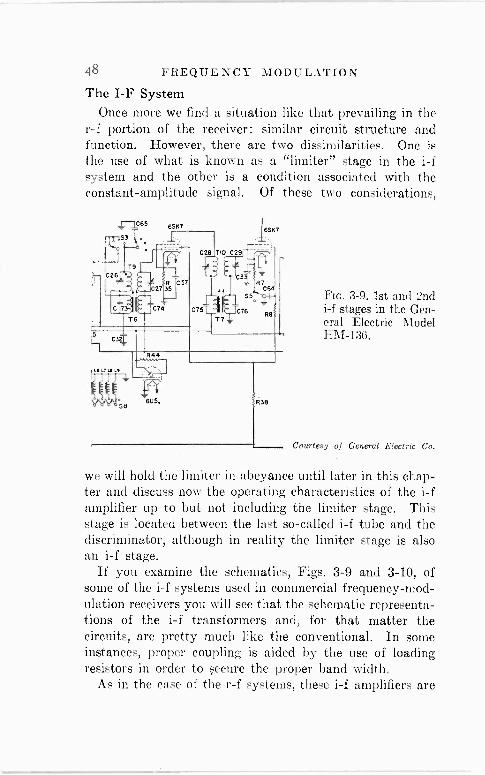
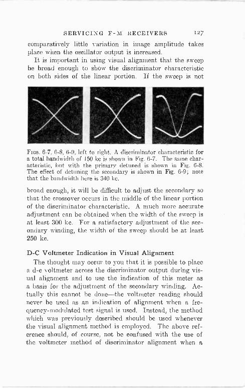
One of the differences is found in the design of the r -f and i -f circuits. Not that the f -m receiver r -f and i -f sys- tems look different upon paper from the representation of the a -m receiver, but the physical design of the transform- ers is different in order to provide the proper band pass. This is more particularly true in the case of the i -f ampli- fier than in the r -f system, because the ratio of the band- width to the actual resonant frequency is much greater in the former than in the latter. Whereas the general run of i -f systems in the conventional broadcast type of super- heterodyne used so far for a -m reception operates with an i -f peak of from 175 kc to about 465 kc and a band width òf approximately 10 kc, the f -m receiver employs an i -f peak of from 1.5 me to perhaps 10 me and a band width of about 150 kc or 75 kc each side of the i -f peak. This is
used to transmit an audio range of about 15,000 cycles. As a part of the i -f system and operating at the i -f peak
FREQUENCY MODULATION 9
is a stage identified as a "limiter." This is not entirely new to superheterodynes in that it was used in a double super- heterodyne manufactured several years ago. The general and basic function of this limiter stage is to maintain the carrier amplitude constant over the operating range of the receiver. Although much more is to follow later in this volume, we can say here that the limiter stage comes into play at the lowest input signal level at the antenna that would represent normal operation. Another stage which is vital in a f -m receiver is the "discriminator," but this tube too is not new to the service industry, in that it is used in every a -f -c receiver for the purpose of developing the con- trol voltage for the a -f -c control tube and sometimes de- modulating the i -f signal.
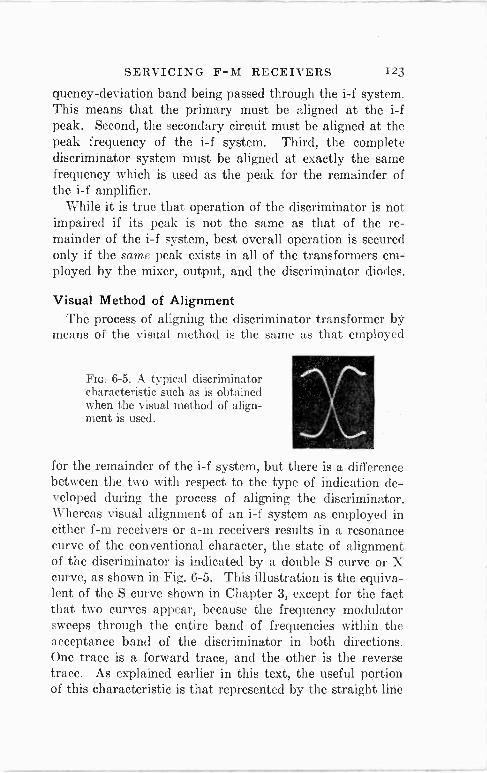
Of course signal distribution in the f -m receiver is like that in any other receiver, as will be discussed later in this volume, and signal tracing, if we inject the thought at this moment, is applicable to the f -m receiver. Now it is possible that as a result of what has been said about the presence of a constant amplitude carrier in the receiver, that some might think that this carrier remains constant without any amplification. Such is not the case. The normal form of amplification takes place in all of the r -f, mixer and i -f tubes, just as if the signal were amplitude modulated, be- cause after all is said and done, the function of the vacuum tube as an amplifier remains the same for f -m and a -m types of modulated carriers. This, too, will be discussed at greater length later.
Once past the discriminator, the receiver is identical to those already in use. Perhaps because of the higher audio range used with the frequency -modulated form of trans- mission, these will have high fidelity audio systems, but as far as operation is concerned, one audio system is like the other. Whatever special features relating to ease of opera- tion and convenience, which may be found in a -m type receivers, will no doubt make their appearance in f -m re- ceivers, and are handled in the conventional manner.
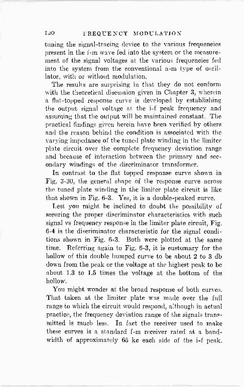
FREQUENCY MODULATION
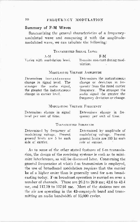
Summary of F -M Waves Summarizing the general characteristics of a frequency -
modulated wave and comparing it with the amplitude - modulated wave, we can tabulate the following:
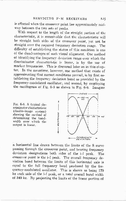
TRANSMITTED SIGNAL LEVEL
A -M F -M Varies with modulation level. Remains constant during mod-
ulation.
MODULATING VOLTAGE AMPLITUDE
Determines instantaneous change in signal level. The stronger the audio signal, the greater the instantaneous change in carrier level.
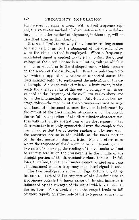
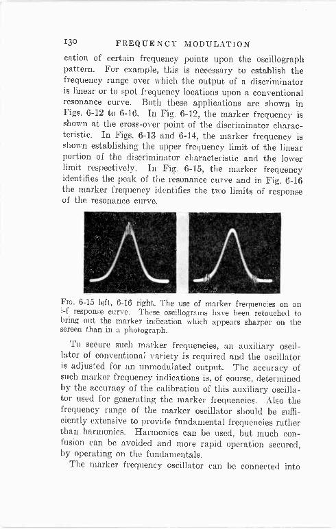
Determines the instantaneous change or deviation in fre- quency from the rated carrier frequency. The stronger the audio signal the greater the frequency deviation or change.
MODULATING VOLTAGE FREQUENCY
Determines change in signal level per unit of time.
TRANSMITTE
Determined by frequency of modulating voltage. Present general limits are 5 kc each side of carrier.
Determines change in fre- quency per unit of time.
D SIDEBANDS
Determined by amplitude of modulating voltage. Present general limits are 100 kc each side of carrier.
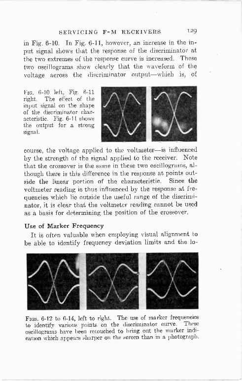
As to some of the other stated features of f -m transmis- sion, the design of the receiving systems is such as to mini- mize interference, as will be discussed later. Concerning the general frequencies at which f -m transmission is employed, the use of broadband modulation requires that the carrier be of a higher order than is generally used for a -m broad- casting today. F -m broadcast operation is carried on over a number of channels. These are 26.3 to 26.9 mc; 42.6 to 43.4 mc, and 117.19 to 117.91 mc. Most of the stations now on the air are operating in the 43 -megacycle band and trans- mitting an audio bandwidth of 15,000 cycles.
Chapter II
WHAT HAPPENS AT THE TRANSMITTER
WE HAVE discussed in general the difference between frequency -modulated and amplitude -modulated waves. Let us now delve a little deeper and see
what happens during the formation of the frequency -modu- lated wave so as to understand more completely the compo- sition of the wave, for what it may be worth when we consider the operation and servicing of the f -m receiver.
There are a number of different ways of producing a fre- quency -modulated wave, in fact every serviceman who has employed the visual or oscillographic method of alignment of an intermediate -frequency amplifier has utilized a fre- quency -modulated carrier. We are referring to the various frequency modulators developed several years ago for use by the servicing industry. You might recall that these were of the electronic type and also of the rotating condenser variety. Unfortunately however, very few descriptions of the formation of the resultant wave produced by these de- vices made the radio press. But we cannot help recall that three or four different arrangements were used by different manufacturers to produce the same final result, that is, the same final output wave for testing purposes.
A similar situation exists in the broadcasting field. There are several ways of producing the final frequency -modulated carrier and while in detail these systems differ, in the final result they are the same. This being the case and since the servicing industry is interested in the subject of frequency modulation more from the viewpoint of the receiver than the transmitter, we feel that the description of the trans -
ii
I2 FREQUENCY MODULATION
mitter operation need not cover in full and complete detail each and every one of the arrangements. Therefore we are going to devote most of our attention, perhaps even depart- ing from exact preciseness of detail, to that arrangement which lends itself to easiest comprehension, yet does provide a clear idea of what constitutes the frequency -modulated wave.
Simplest Frequency Modulator We made mention of the frequency modulators employed
during service operations. In some of these' the frequency is varied by a motor -driven rotating variable condenser, the idea being to cause a change in frequency between any two desired limits. Usually, with arrangements of this kind the total bandwidth covered may be from a few percent to per- haps ten percent of the mean frequency. The amplitude of the wave is constant over the entire range and the speed of rotation represents the audio frequency, or the time rate of change in frequency. The item of audio amplitude which would determine the amount of frequency deviation does not enter into the operation of this arrangement. Other well known systems employ a vacuum tube as a fictitious inductance, which inductance is in effect across the coil in the tuned circuit of the oscillator. More about this system will be given later, because an elaboration of the method is actually used in one type of frequency -modulated broadcast transmitter.
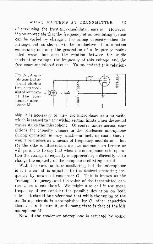
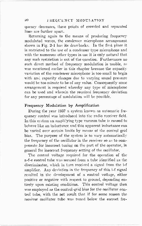
Bearing in mind the possibility of varying the frequency of a tuned oscillator circuit by changing either the capacity or the inductance, we can proceed with the discussion of what is actually the simplest type of frequency modulator resembling the operation of a broadcast transmitter. This is shown in Fig. 2-1, wherein a condenser -type microphone M is shunted directly across the tuning condenser C of a simple oscillator.
This circuit is not intended to convey the idea that this is the type of oscillating system actually used in the trans- mitter, or that which we shall describe is the exact method
WHAT HAPPENS AT TRANSMITTER 13
of producing the frequency -modulated carrier. However, if you appreciate that the frequency of an oscillating system can be varied by changing the tuning capacity then the arrangement as shown will be productive of information concerning not only the generation of a frequency -modu- lated wave, but also the relation between the audio modulating voltage, the frequency of this voltage, and the frequency -modulated carrier. To understand this relation -
Fm. 2-1. A sim- ple oscillator circuit which is frequency mod- ulated by means of the con- denser micro- phone M.
ship it is necessary to view the microphone as a capacity which is caused to vary within certain limits when the sound waves strike the microphone. Of course, under normal con- ditions the capacity change in the condenser microphone during operation is very small-in fact, so small that it would be useless as a means of frequency modulation-but for the sake of illustration we can assume such license as will permit us to say that when the microphone is in opera- tion the change in capacity is appreciable; sufficiently so to change the capacity of the complete oscillating circuit.
With the vacuum tube oscillating, but the microphone idle, the circuit is adjusted to the desired operating fre- quency by means of condenser C. This is known as the "resting" frequency, and the value of the transmitted car- rier when unmodulated. We might also call it the mean frequency if we consider the possible deviation on both sides. It should be understood that while the tuning of the oscillating circuit is accomplished by C, other capacities also exist in the circuit, and among these is that of the idle microphone M.
Now, if the condenser microphone is actuated by sound
14 FREQUENCY MODULATION
waves, as shown in Fig. 2-2, the diaphragm will vibrate to and fro, thus varying the space between it and the station- ary plate. Since the capacity of the microphone is depend- ent upon the spacing between the movable and stationary plates, any movement of the diaphragm, that is, the mova- ble plate, will change the spacing, hence the capacity. If, as a result of a sound wave applied to the microphone, the movable plate is caused to move or shift inward towards the stationary plate, the spacing is reduced and conse- quently the capacity of the microphone is increased. If, on the other hand, the movable plate is caused to move out- ward-away from the stationary plate, the spacing will be increased and consequently the capacity will be decreased. The arrows and + and - signs in Fig. 2-2 indicate this condition. The to and fro motion of the movable plate is the natural action when a sound is applied to the micro- phone.
304/NO IVA VED
MOVADLE STAT/ONA.QY O/APNRA6M PLATE
OU7PU7
FIG. 2-2. The sound waves striking the diaphragm of the mi- crophone cause the ca- pacity to change in accordance with the sound vibrations.
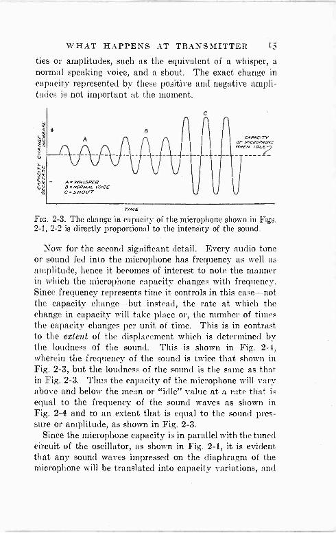
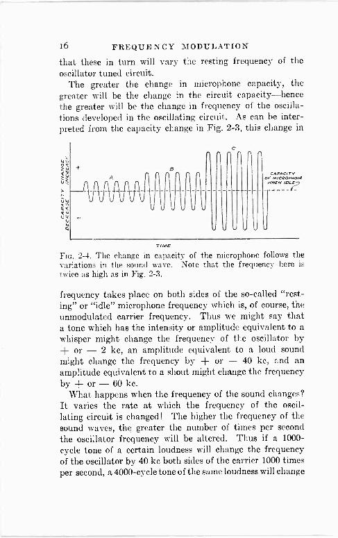
Another very significant detail is the manner in which this capacity changes with respect to the audio signal applied to the microphone. It can be readily seen that the stronger the audio signal, the greater the sound pressure applied to the microphone, hence the greater will be the movement or displacement of the movable plate from its normal idle position-both towards and away from the stationary plate. Expressed differently, the louder the sound, the greater is the actual change in capacity. This is illustrated in Fig. 2-3, wherein you see the change in microphone capacity for three sounds of the same frequency but of different intensi-
WHAT HAPPENS AT TRANSMITTER 15
ties or amplitudes, such as the equivalent of a whisper, a normal speaking voice, and a shout. The exact change in capacity represented by these positive and negative ampli- tudes is not important at the moment.
C
+ g
A
^ - WH/JPEQ D -NORMAL VO/CE .
C-5NOUT
CAPACITY OP MICROPHONE WHEN IOLE -j
TIME
Fm. 2-3. The change in capacity of the microphone shown in Figs. 2-1, 2-2 is directly proportional to the intensity of the sound.
Now for the second significant detail. Every audio tone or sound fed into the microphone has frequency as well as amplitude, hence it becomes of interest to note the manner in which the microphone capacity changes with frequency. Since frequency represents time it controls in this case-not the capacity change-but instead, the rate at which the change in capacity will take place or, the number of times the capacity changes per unit of time. This is in contrast to the extent of the displacement which is determined by the loudness of the sound. This is shown in Fig. 2-4, wherein the frequency of the sound is twice that shown in Fig. 2-3, but the loudness of the sound is the same as that in Fig. 2-3. Thus the capacity of the microphone will vary above and below the mean or "idle" value at a rate that is equal to the frequency of the sound waves as shown in Fig. 2-4 and to an extent that is equal to the sound pres- sure or amplitude, as shown in Fig. 2-3.
Since the microphone capacity is in parallel with the tuned circuit of the oscillator, as shown in Fig. 2-1, it is evident that any sound waves impressed on the diaphragm of the microphone will be translated into capacity variations, and
16 FREQUENCY MODULATION
that these in turn will vary the resting frequency of the oscillator tuned circuit.
The greater the change in microphone capacity, the greater will be the change in the circuit capacity-hence the greater will be the change in frequency of the oscilla- tions developed in the oscillating circuit. As can be inter- preted from the capacity change in Fig. 2-3, this change in
B r
1 J
J
r
CAPACITY OF MICROPHONE
WHEN
TIME
Fm. 2-4. The change in capacity of the microphone follows the variations in the sound wave. Note that the frequency here is twice as high as in Fig. 2-3.
frequency takes place on both sides of the so-called "rest- ing" or "idle" microphone frequency which is, of course, the unmodulated carrier frequency. Thus we might say that a tone which has the intensity or amplitude equivalent to a whisper might change the frequency of the oscillator by + or - 2 kc, an amplitude equivalent to a loud sound might change the frequency by + or - 40 kc, and an amplitude equivalent to a shout might change the frequency by -I- or - 60 kc.
What happens when the frequency of the sound changes? It varies the rate at which the frequency of the oscil- lating circuit is changed! The higher the frequency of the sound waves, the greater the number of times per second the oscillator frequency will be altered. Thus if a 1000 -
cycle tone of a certain loudness will change the frequency of the oscillator by 40 kc both sides of the carrier 1000 times per second, a 4000 -cycle tone of the same loudness will change
WHAT HAPPENS AT TRANSMITTER 17
the frequency of the oscillator by 40 kc, 4000 times per second, and a 200 -cycle tone of like loudness will change the frequency of the oscillator by 40 kc 200 times per sec- ond. Thus, the arrangement shown in Fig. 2-1 satisfies the basic requirements of an f -m transmitter, since both sound pitch and sound amplitude are translated into variations in frequency.
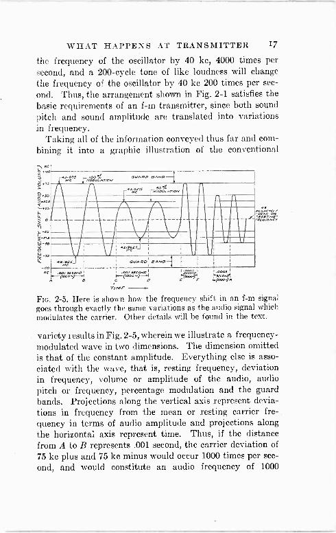
Taking all of the information conveyed thus far and com- bining it into a graphic illustration of the conventional
FIG. 2-5. Here is shown how the frequency shift in an f -m signal goes through exactly the same variations as the audio signal which modulates the carrier. Other details will be found in the text.
variety results in Fig. 2-5, wherein we illustrate a frequency - modulated wave in two dimensions. The dimension omitted is that of the constant amplitude. Everything else is asso- ciated with the wave, that is, resting frequency, deviation in frequency, volume or amplitude of the audio, audio pitch or frequency, percentage modulation and the guard bands. Projections along the vertical axis represent devia- tions in frequency from the mean or resting carrier fre- quency in terms of audio amplitude and projections along the horizontal axis represent time. Thus, if the distance from A to B represents .001 second, the carrier deviation of
75 kc plus and 75 ke minus would occur 1000 times per sec- ond, and would constitute an audio frequency of 1000
i8 FREQUENCY MODULATION
cycles. Since the carrier deviation covers the complete range of shift permitted under present standards, it repre- sents 100 percent modulation. Again we want to mention the possibility that in time to come 100 percent modulation may represent 60 kc deviation or some other value instead of 75 kc deviation shown in Fig. 2-5.
7/ME.
¡III 111111
1111 Ì111111111
IIII Hill,
In 111 111
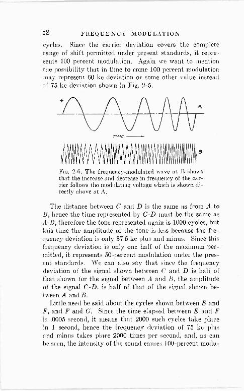
FIG. 2-6. The frequency -modulated wave at B shows that the increase and decrease in frequency of the car- rier follows the modulating voltage which is shown di- rectly above at A.
The distance between C and D is the same as from A to B, hence the time represented by C -D must be the same as A -B, therefore the tone represented again is 1000 cycles, but this time the amplitude of the tone is less because the fre- quency deviation is only 37.5 kc plus and minus. Since this frequency deviation is only one half of the maximum per- mitted, it represents 50 -percent modulation under the pres- ent standards. We can also say that since the frequency deviation of the signal shown between C and D is half of that shown for the signal between A and B, the amplitude of the signal C -D, is half of that of the signal shown be- tween A and B.
Little need be said about the cycles shown between E and F, and F and G. Since the time elapsed between E and F is .0005 second, it means that 2000 such cycles take place in 1 second, hence the frequency deviation of 75 kc plus and minus takes place 2000 times per second, and, as can be seen, the intensity of the sound causes 100 -percent modu-
WHAT HAPPENS AT TRANSMITTER 19
lation. The tone between G and H is of the same fre- quency as that between E and F, but the amplitude is less; that is, it is not as loud. Hence the frequency deviation is only 50 kc plus and minus and represents according to pres- ent day standards a modulation of 66 percent.
It would be possible to illustrate many more examples of audio frequency and signal frequency deviation or audio amplitude but it is not deemed necessary, because from what is illustrated you can certainly gather the general structure of a frequency -modulated wave. You can readily under- stand from Fig. 2-5 that if any audio tone is held constant for a while in both pitch and amplitude, the appearance of the wave, if shown in such graphic form, would resemble an unmodulated carrier with upper and lower frequency limits representing the frequency deviation caused by the amplitude of the audio wave.
We cannot at this time embark upon another subject without first referring if only briefly to another representa- tion of a frequency -modulated carrier, one which has ap- peared in print and which appears like a condensation and rarefaction of vertical lines. This illustration which, al- though not designated as such is shown with respect to time, is the equivalent of viewing the frequency -modulated wave in Fig. 2-5 from the top, that is looking down on the top of the cycle drawings. In Fig. 2-6 the positive peaks of the audio curve A, because of the circuit structure, are assumed io increase the frequency; hence the number of signal cycles on curve B is greater per unit of time with respect to the number which occurs when the modulation is zero. This in- creased number of cycles naturally crowds the lines, as shown in B.
On the negative audio peaks the frequency deviation is on the minus side, hence a fewer number of signal cycles occur in the same unit of time and the lines are further apart. As the audio or modulating frequency increases you will note that the points of crowded and widely separated lines are closer together and more numerous for any unit time, shown along the horizontal axis. As the audio fre-
20 FREQUENCY MODULATION
quency decreases, these points of crowded and separated lines are further apart.
Returning again to the means of producing frequency modulated waves, the condenser microphone arrangement shown in Fig. 2-1 has its drawbacks. In the first place it is restricted to the use of a condenser type microphone and with the numerous other types in use it is only natural that any such restriction is out of the question. Furthermore no such direct method of frequency modulation is usable, as was mentioned earlier in this chapter because the capacity variation of the condenser microphone is too small to begin with and capacity changes due to varying sound pressure would be too minute to be of any value. Consequently some arrangement is required whereby any type of microphone can be used and wherein the required frequency deviation for any percentage of modulation will be possible.
Frequency Modulation by Amplification During the year 1937 a system known as automatic fre-
quency control was introduced into the radio receiver field. In this system an amplifying type vacuum tube is caused to behave like an inductance and this apparent inductance can be varied over certain limits by means of the control grid bias. The purpose of the system is to vary automatically the frequency of the oscillator in the receiver so as to com- pensate for incorrect tuning on the part of the operator, in general for incorrect frequency setting of the oscillator.
The control voltage required for the operation of the a -f -c control tube was secured from a tube identified as the discriminator, which in turn received a signal from the i -f amplifier. Any deviation in the frequency of this i -f signal resulted in the development of a control voltage, either positive or negative with respect to ground, depending en- tirely upon existing conditions. This control voltage then was employed as the control -grid bias for the oscillator con- trol tube, with the net result that if for some reason .the receiver oscillator tube was tuned below the correct fre-
WHAT HAPPENS AT TRANSMITTER 2I
quency or above the correct frequency, automatic correction was obtained by electronic means.
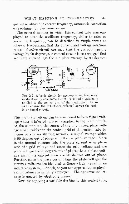
The general manner in which this control tube was em- ployed to alter the oscillator frequency, either to raise or lower the frequency, can be described in simple terms as follows: Recognizing that the current and voltage relations in an inductive circuit are such that the current lags the voltage by 90 degrees, the control circuit is so arranged that a -c plate current lags the a -c plate voltage by 90 degrees.
OSC.
FIG. 2-7. A basic circuit for accomplishing frequency modulation by electronic means. The audio voltage is applied to the control grid of the modulator tube so as to change the inductance reflected across the oscil- lator tuned circuit.
This a -c plate voltage can be considered to be a signal volt- age which is injected into or is applied to the plate circuit. At the same time, the source of the alternating plate volt- age also furnishes to the control grid of the control tube by means of a phase shifting network, a signal voltage which is 90 degrees out of phase with the a -c plate voltage. Since in the normal vacuum tube the plate current is in phase with the grid voltage and since the grid voltage and a -c plate voltage are 90 degrees out of phase, the a -c plate volt- age and plate current then are 90 degrees out of phase. Further, since the plate current lags the plate voltage, the circuit conditions are identical to those which prevail in an inductive system, although, as you can appreciate, no physi- cal inductance is actually employed. The apparent induct- ance is created by electronic means.
Now, by applying a variable d -c bias to this control tube,
22 FREQUENCY MODULATION
it is possible to vary the magnitude of the plate current and this variation in plate current is tantamount to varying the value of the apparent inductance. Thus, if the plate current is increased, it is the equivalent of having reduced the value of the apparent inductance. On the other hand if the plate current is decreased as a result of the control -grid bias, it is the equivalent of having increased this apparent induct- ance. In other words, the plate circuit of this control tube behaves as an automatically controlled variable inductance, or if we wish to identify it differently, it acts like a variable inductive reactance.
By connecting the plate circuit of this control tube across the tuned circuit of the oscillator, automatic control of the frequency is accomplished. The exact manner in which the required control voltage is developed in such a circuit is not of moment at this time, other than to say that a similar arrangement is employed in receivers intended for the re- ception of frequency -modulated signals.
If you now can picture the application of an audio volt- age as the control -grid bias for the control tube and this control tube governs the frequency of the oscillator you have a picture of how frequency modulation can be accomplished with any type of microphone and by utilizing the amplifying property of a vacuum tube. The frequency of the audio voltages employed as the control grid bias voltage for the control tube determines the rate of frequency shift and the magnitude of these audio voltages determines the extent of the change in frequency.
This arrangement for increasing the range of frequency shift and permitting the use of any type of microphone, is shown in the block diagram of Fig. 2-8. The microphone output is fed through a pre -amplifier and the resultant audio voltage applied to the control tube or variable -reactance modulator. The control tube alters the effective inductance of the oscillator tank circuit, and therefore causes frequency changes that are proportional to modulation amplitude.
WHAT HAPPENS AT TRANSMITTER 23
One of the requirements of wide -band frequency modu- lation is that the frequency variations shall be symmetrical with respect to the mean frequency, pass through it, and return exactly to the carrier figure when modulation stops. A prime requisite, then, is that, after such excursions, the carrier frequency must always return to the same mean value.
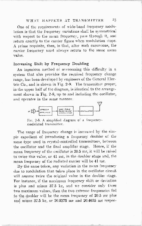
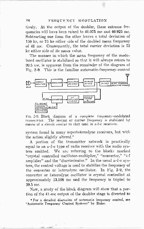
Increasing Shift by Frequency Doubling An ingenious method of overcoming this difficulty in a
system that also provides the required frequency change range, has been developed by engineers of the General Elec- tric Co., and is shown in Fig. 2-9. The transmitter proper, in the upper half of the diagram, is identical to the arrange- ment shown in Fig. 2-8, up to and including the oscillator, and operates in the same manner.
M SPEECH AMPLIFIER
VAR/ABLE REACTANCE MODULATOR
OSC/LCATOR
FIG. 2-8. A simplified diagram of a frequency - modulated transmitter.
The range of frequency change is increased by the sim- ple expedient of introducing a frequency doubler of the same type used in crystal -controlled transmitters, between the oscillator and the final amplifier stage. Hence, if the mean frequency of the oscillator is 20.5 mc, it will be raised tó twice this value, or 41 mc, in the doubler stage and, the mean frequency of the radiated carrier will be 41 mc.
By the same token, any variation in the mean frequency due to modulation that takes place in the oscillator circuit will assume twice the original value in the doubler stage. For instance, if thé maximum frequency shift or deviation is plus and minus 37.5 kc, and we consider only these two maximum values, then the two extreme frequencies fed to the doubler will be the mean frequency of 20.5 mc plus and minus 37.5 kc, or 20.5375 mc and 20.4625 mc respec-
24 FREQUENCY MODULATION
tively. At the output of the doubler, these extreme fre- quencies will have been raised to 41.075 mc and 40.925 mc. Subtracting one from the other leaves a total deviation of 150 kc, or 75 kc either side of the doubled mean frequency of 41 mc. Consequently, the total carrier deviation is 75
kc either side of its mean value. The manner in. which the mean frequency of the modu-
lated oscillator is stabilized so that it will always return to 20.5 mc, is apparent from the remainder of the diagram of Fig. 2-9. This is the familiar automatic -frequency -control
NPEeCv w MirrE
-1" OOULATOR C/A (ZOáMC) DOUBLER (a/ Mc) nC)
a/MC 1-F - CONYERTCR-a. AMGG/FIER (/.SMC)
(/3. /BC MC)
CRYSTAL sC O!C/L[A DE MULI/FC/CR
F O/SCR/M- /vATOR
dr OE ECTOR
4i.r+C CARRIER (REST/.v6 VALVE)
FIG. 2-9. Block diagram of a complete frequency -modulated transmitter. The resting or carrier frequency is stabilized by means of a circuit similar to that used in a -f -c receivers.
system found in many superheterodyne receivers, but with the action slightly altered.*
A portion of the transmitter network is practically equal to an a -f -c type of radio receiver with the audio sys- tem omitted. We are referring to the blocks marked "crystal controlled oscillator -multiplier," "converter," "i -f amplifier" and the "discriminator." In the usual a -f -c sys- tem, the control voltage is used to. stabilize the frequency of the converter or heterodyne oscillator. In Fig. 2-9, the converter or heterodyne oscillator is crystal controlled at approximately 13.166 mc and the frequency is tripled to 39.5 mc.
Now, a study of the block diagram will show that a por- tion of the 41 -mc output of the doubler stage is diverted to
* For a detailed discussion of automatic frequency control, see "Automatic Frequency Control Systems" by Rider.
WHAT HAPPENS AT TRANSMITTER 25
the converter of the frequency -stabilization system, where it beats with the 39.5 -mc crystal -controlled oscillator volt- age, producing an intermediate frequency of 1.5 mc. This latter voltage is amplified in the i -f stage, passed through the frequency -discriminator, and rectified. The resultant d -c voltage, as previously mentioned, is applied to the con- troI element of the modulator tube and serves as its normal bias.
The discriminator control voltage is applied to the same control element of the modulator tube to which is fed the audio modulation. Since the modulator tube is made to function as a variable inductance in parallel with the oscil- lator tank circuit, it has exactly the same action and char- acteristics as the oscillator control tube in a receiver a -f -c system, and controls or stabilizes the transmitter oscillator carrier frequency at 41 mc.
The time constant of the filter in the d -c bias voltage circuit feeding the control tube (modulator) is made large so that the frequency -stabilization system will be slow act- ing and thereby be unaffected by the audio modulation volt- age; otherwise the frequency -stabilization system would have a compensating effect on frequency variations due to modulation, as well as on variations of the oscillator's mean frequency due to drift, etc.
It is obvious from the foregoing that any tendency on the part of the transmitter oscillator to depart from its mean frequency for any reason other than that caused by audio modulation, will be automatically compensated for by a re- sultant change in the value of the d -c control voltage from the discriminator. The result is a stable carrier which re- turns to its original frequency after having traveled through its excursions due to modulation.
The Armstrong System Another method of producing a frequency -modulated
wave is that of Major E. H. Armstrong, wherein a phase shift is the basis of the final frequency -modulated wave, and, when the system is spoken of, it is referred to as phase
26 FREQUENCY MODULATION
modulation. However, in view of the fact that the final re- sultant of this system of operation is a frequency -modulated wave of conventional character, it can be said that phase modulation and frequency modulation are one and the same. Or, to say the least, phase modulation is one form of frequency modulation.
Recognizing the purpose of this volume-namely, a dis- cussion of frequency modulation from the viewpoint of the servicing industry-we do not deem it fitting to include the mathematical treatment of phase modulation. And, inci- dentally, a great deal of such treatment is associated with phase modulation. However, it is necessary to include in this book some discussion of how phase modulation can re- sult in a frequency -modulated output wave-just as we
. described in simple terms the production of a frequency - modulated wave by the variation of C and L in an oscillator system. In this presentation we want it known that we depart from preciseness in that the references to phase shift and the equivalent change in frequency are expressed in simple terms and are those which will facilitate comprehen- sion of how a shift in phase is equal to a change in fre- quency.
Before describing the actual highlights and features of the Armstrong system as used in a complete transmitter, let us consider some facts associated with phase shift and equivalent change in frequency. The numerical figures quoted in these examples are purely illustrative and are not intended to convey the impression that these are the nu- merical values actually used in practice, or that the simpli- fied methods of operation as described are identical to those employed in a phase -modulated transmitting system. The illustrations given are much simpler than the actual process used, but this should not interfere with the final application of the information given in these pages. Our main objec- tive, as can be readily understood, is maintenance of the re- ceiver and a general picture of the manner of producing the wave which is acted upon by the receiver, is sufficient be- cause when we speak about the operation of the receiver,
WHAT HAPPENS AT TRANSMITTER 27
we are in no way limited in action by the manner in which the basic signal is produced at the transmitter. 'Whether the signal is produced by phase modulation or by what we can call direct frequency modulation, the final output of the receiver is the same. Furthermore, the service problems as- sociated with the receiver are not determined by the exact method of production of the frequency -modulated wave.
Phase Shift and Frequency Shift You might ask, what does phase shift have to do with
frequency modulation? It has a great deal to do with it because, as you will see, when we shift the phase of one component of a wave with respect to the other component, we are in effect changing the frequency of one with respect to the other. What we mean is as follows:
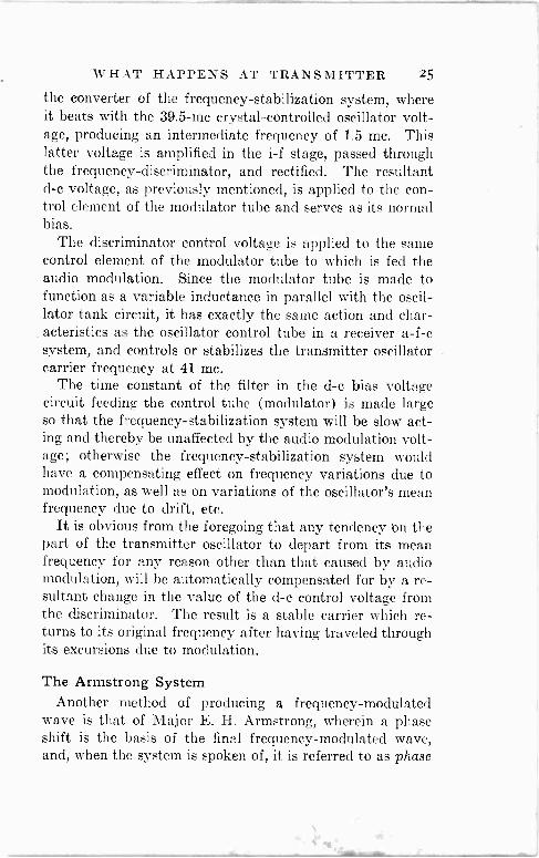
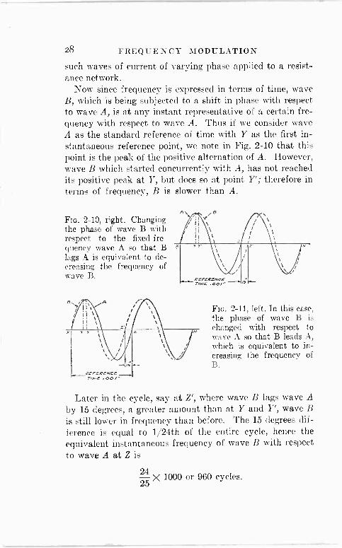
Suppose that you imagine two sine waves A and B, each of 1000 cycles and secured from two different sources. Let us further imagine that we apply these two currents to a common resistive circuit, but by some means, after having started the two waves in phase, we change the phase of B by varying degrees until B lags A by a maximum of 15 de- grees. This is shown in Fig. 2-10.
If you analyse this drawing you will note that the time required for the completion of a cycle of A is indicated upon the time axis as the reference time of .001 second. Now when we change the phase of one wave with respect to an- other and one wave lags the other, it means that the second wave moves through whatever reference points are selected after the first; therefore we can say that wave B at any in- stant is slower than wave A. This is evident in Fig. 2-10 and so is the fact that wave B slows down more and more as it approaches the completion of its cycle.
At first glance such a phenomenon appears confusing, but if you recognize that phase shifting circuits are available and that wave A is secured from one source and wave B is secured from another source and B is passed through a vari- able delay network, we can visualize the presence of two
28 FREQUENCY MODULATION
such waves of current of varying phase applied to a resist- ance network.
Now since frequency is expressed in terms of time, wave B, which is being subjected to a shift in phase with respect to wave A, is at any instant representative of a certain fre- quency with respect to wave A. Thus if we consider wave A as the standard reference of time with Y as the first in- stantaneous reference point, we note in Fig. 2-10 that this point is the peak of the positive alternation of A. However, wave B which started concurrently with A, has not reached its positive peak at Y, but does so at point Y'; therefore in terms of frequency, B is slower than A.
FIG. 2-10, right. Changing the phase of wave B with respect to the fixed -fre- quency wave A so that B lags A is equivalent to de- creasing the frequency of wave B.
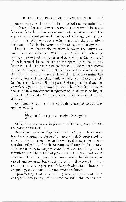
FIG. 2-11, left. In this case, the phase of wave B is changed with respect to wave A so that B leads A, which is equivalent to in- creasing the frequency of B.
Later in the cycle, say at Z', where wave B lags wave A
by 15 degrees, a greater amount than at Y and Y', wave B
is still lower in frequency than before. The 15 degrees dif- ference is equal to 1/24th of the entire cycle, hence the equivalent instantaneous frequency of wave B with respect to wave A at Z is
24 25 X
1000 or 960 cycles.
WHAT HAPPENS AT TRANSMITTER 29
As we advance further in the illustration, we note that the phase difference between wave A and wave B becomes less and less, hence in accordance with what was said the equivalent instantaneous frequency of B is increasing, un- til, at point N, the waves are in phase and the equivalent frequency of B is the same as that of A, or 1000 cycles.
Let us now change the relation between the waves we have been considering. With wave A still the reference wave, suppose that we again gradually change the phase of B with respect to A, but this time speed up B, so that it leads wave A. This is shown in Fig. 2-11, where both waves A and B being still rated at 1000 cycles each, are in phase at X, but at Y and Y' wave B leads A. If you examine the curves, you will find that while wave A completes a cycle in .001 second, wave B has passed through more than one complete cycle in the same period; therefore it stands to reason that whatever the frequency of B, it must be higher than A. At points Z and Z', wave B leads wave A by 15
degrees. At points Z and Z', the equivalent instantaneous fre-
quency of B is
24 23 X 1000 or approximately 1042 cycles.
At N, both waves are in phase and the frequency of B is the same at that of A.
Referring again to Figs. 2-10 and 2-11, you have seen how by changing the phase of a wave, which is equivalent to slowing down or speeding up the wave, it is possible to cre- ate the equivalent of an instantaneous change in frequency. With what is to follow, we want to stress that the greatest significance of the examples given lies not in the presence of a wave of fixed frequency and one wherein the frequency is raised and lowered, but the latter only. However, to illus- trate properly how phase shift is equivalent to a change in frequency, a standard reference wave is shown.
Appreciating that a shift in phase is equivalent to a change in frequency, let us now consider the means em-
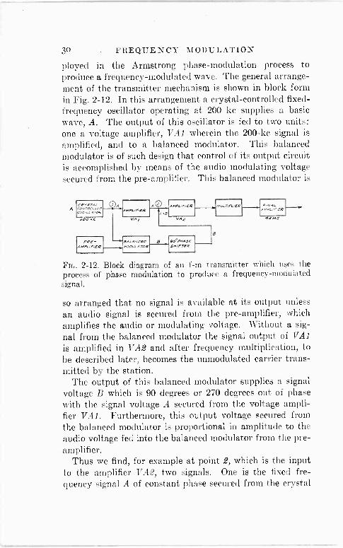
30 FREQUENCY MODULATION
ployed in the Armstrong phase -modulation process to produce a frequency -modulated wave. The general arrange- ment of the transmitter mechanism is shown in block form in Fig. 2-12. In this arrangement a crystal -controlled fixed - frequency oscillator operating at 200 kc supplies a basic wave, A. The output of this oscillator is fed to two units: one a voltage amplifier, VA1 wherein the 200-kc signal is
amplified, and to a balanced modulator. This balanced modulator is of such design that control of its output circuit is accomplished by means of the audio modulating voltage secured from the pre -amplifier. This balanced modulator is
VA AO AMP4/iFR u..nPc/FR CaMr57.41_
A ROceo 03C,,,7-04AMPG///FR A 9 AMP/2R
200 KC VA / VA2 42 MC
PQ6- AMP4P/6R
EA[ALC6Q B 90 PNA,C SNIP7MR
FIG. 2-12. Block diagram of an f -m transmitter which uses the process of phase modulation to produce a frequency -modulated signal.
so arranged that no signal is available at its output unless an audio signal is secured from the pre -amplifier, which amplifies the audio or modulating voltage. Without a sig- nal from the balanced modulator the signal output of VA1
is amplified in VA2 and after frequency multiplication, to be described later, becomes the unmodulated carrier trans- mitted by the station.
The output of this balanced modulator supplies a signal voltage B which is 90 degrees or 270 degrees out of phase with the signal voltage A secured from the voltage ampli- fier VA1. Furthermore, this output voltage secured from the balanced modulator is proportional in amplitude to the audio voltage fed into the balanced modulator from the pre- amplifier.
Thus we find, for example at point 2, which is the input to the amplifier VA2, two signals. One is the fixed fre- quency signal A of constant phase secured from the crystal
WHAT HAPPENS AT TRANSMITTER 31
oscillator and amplified by amplifier VAl; the other is a signal B secured from the balanced modulator system. This signal B is 90 or 270 degrees out of phase with signal A and this difference in phase represents a lag or lead of B with respect to A. When B is 90 degrees out of phase with A, it lags A and when B is 270 degrees out of phase with A, it leads A. Of interest is the fact this phase difference always is either 90 or 270 degrees, depending upon the polarity of the audio voltage fed into the modulator, which in turn means the polarity of the voltage secured from the balanced modulator.
At this stage you may wonder about the frequency of the signal secured from the balanced modulator. Essentially this signal is a 200-kc signal of a certain definite phase but varying in amplitude in accordance with the differential voltage developed in the modulator plate circuit.
Now we must recognize one very important condition which exists at the input of amplifier VA2. The only time that voltage B exists at this point is when an audio voltage is applied to the balanced modulator, therefore it is signifi- cant to realize that this voltage B, which is of fixed phase with respect to the unmodulated carrier A, also varies in amplitude in accordance with the amplitude of the modu- lating voltage. Thus there exists at the input of amplifier VA2, one voltage A, the unmodulated carrier, and a voltage B of varying amplitude and polarity and either a 90 or a 270 -degree phase difference between B and A. The com- bination of both of these voltages results in a final output wave which is frequency modulated.
In view of the statement that the phase difference be- tween A and B when they are combined in amplifier VA2 is fixed at. either 90 or 270 degrees, you might wonder about how or why the frequency of the final output wave varies. This is due to the fact that what can be described as two distinctly different actions take place. First the combina- tion of waves A and B takes place in a manner determined by the fixed phase difference of 90 or 270 degrees. If the voltage of wave B was kept constant, spell as would be ob-
32 FREQUENCY MODULATION
tained if the balanced modulator were unbalanced by a d -c input, the combination of A and B would be a carrier equal in frequency to that of wave A and displaced in phase from both A and B, but of fixed phase which means there will be no frequency variation. However, since the voltage ob- tained from the output of the balanced modulator is varying in amplitude in accordance with the amplitude of the audio input, the combination of A and B is a final wave which varies in phase as long as the modulating voltage is being applied to the modulator input. The instantaneous varia -
O
MOOULATEO QF
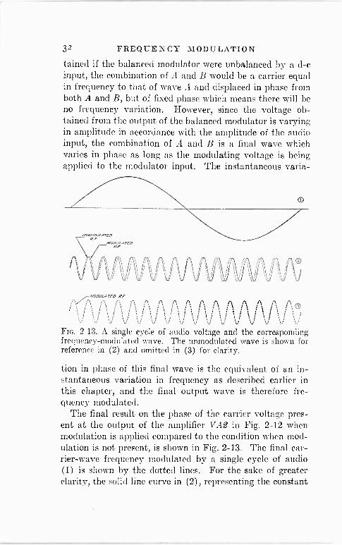
i L` Jj 1i FIG. 2-13. A single cycle of audio voltage and the corresponding frequency -modulated wave. The unmodulated wave is shown for reference in (2) and omitted in (3) for clarity.
tion in phase of this final wave is the equivalent of an in- stantaneous variation in frequency as described earlier in this chapter, and the final output wave is therefore fre- quency modulated.
The final result on the phase of the carrier voltage pres- ent at the output of the amplifier VA2 in Fig. 2-12 when modulation is applied compared to the condition when mod- ulation is not present, is shown in Fig. 2-13. The final car- rier -wave frequency modulated by a single cycle of audio (1) is shown by the dotted lines. For the sake of greater clarity, the solid line curve in (2), representing the constant
WHAT HAPPENS AT TRANSMITTER 33
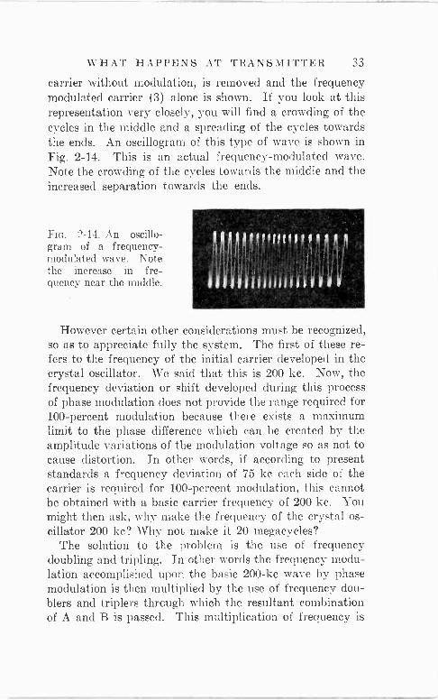
carrier without modulation, is removed and the frequency modulated carrier (3) alone is shown. If you look at this representation very closely, you will find a crowding of the cycles in the middle and a spreading of the cycles towards the ends. An oscillogram of this type of wave is shown in Fig. 2-14. This is an actual frequency -modulated wave. Note the crowding of the cycles towards the middle and the increased separation towards the ends.
FIG. 2-14. An oscillo - gram of a frequency - modulated wave. Note the increase , in fre- quency near the middle.
100 tttttrtttt
l # 1111iJrr
However certain other considerations must be recognized, so as to appreciate fully the system. The first of these re- fers to the frequency of the initial carrier developed in the crystal oscillator. We said that this is 200 kc. Now, the frequency deviation or shift developed during this process of phase modulation does not provide the range required for 100 -percent modulation because there exists a maximum limit to the phase difference which can be created by the amplitude variations of the modulation voltage so as not to cause distortion. In other words, if according to present standards a frequency deviation of 75 kc each side of the carrier is required for 100 -percent modulation, this cannot be obtained with a basic carrier frequency of 200 kc. You might then ask, why make the frequency of the crystal os- cillator 200 kc? Why not make it 20 megacycles?
The solution to the problem is the use of frequency doubling and tripling. In other words the frequency modu- lation accomplished upon the basic 200-kc wave by phase modulation is then multiplied by the use of frequency dou- blers and tripiers through which the resultant combination of A and B is passed. This multiplication of frequency is
34 FREQUENCY MODULATION
carried out a sufficient number of times until the proper fre- quency deviation from the carrier is attained to fill the re- quirement of 75 kc deviation both sides of the carrier for 100 -percent modulation.
Effect of Audio Frequency Upon a Phase -Modulated Wave
If we refer back to the discussion of the arrangement of
the transmitter components, Fig. 2-12, we find the explana- tion of another consideration associated with the phase - modulated type of frequency -modulation system. Whereas in the direct method of frequency modulation discussed earlier in this chapter, the amplitude of the modulation volt- age determined the frequency deviation and the frequency of the modulation voltage determined the time rate of fre- quency deviation, a different condition prevails in the phase -modulation system. In this system, the natural op- eration without corrective measures results in control of the frequency deviation by the amplitude of the modulating voltage and also by the frequency of the modulating volt- age. In fact, the higher the frequency of the modulating voltage, the faster is the time rate of change of the phase shift due to the varying balanced modulator output and the greater is the frequency deviation both sides of the carrier.
Such a condition is highly undesired because it prevents fulfillment of one of the prime requisites of the system, namely, that the amplitude of the detected or rectified cur- rent in the receiver should be proportional to the change in frequency at the transmitter; in other words the amplitude of the modulating voltage should be independent of the rate of change of the transmitted wave or if expressed in terms of the modulating voltage, the frequency thereof.
A corrective network is therefore added to the transmit- ter system and this is not shown in Fig. 2-12. This correc- tive network is located between the pre -amplifier or the source of the modulating voltage and the balanced modu- lator. This input amplifier is so designed that the ampli- fication is inversely proportional to the frequency, that is,
WHAT HAPPENS AT TRANSMITTER 35
the amplification is less as the frequency increases. This arrangement accomplishes the aim of making the angle through which the phase of the transmitted signal is shifted vary inversely with frequency and in this way makes the frequency deviation independent of the modulation fre- quency.
For example, if a modulating voltage of 100 cycles and X amplitude causes a phase shift of such magnitude that a frequency deviation of 10 kc takes place, a modulating voltage of 400 cycles and X, a constant amplitude, will shift the phase through whatever angle is created by the amplitude, four times as fast and will result in a final fre- quency deviation four times as great as that for the 100 - cycle voltage. But if by some means the voltage of the 400 -cycle tone becomes X/4 at the input of the balanced modulator, the final effect of this modulating voltage upon the f -m carrier will be such as to cause a frequency devia- tion equal to the X amplitude at 100 cycles, thus offsetting the effect of the modulating frequency upon the frequency deviation, but the rate of deviation still is present in the final f -m carrier. In this way the frequency deviation is proportional to the amplitude of the modulating voltage. If in another example the modulating voltage is 10,000 cycles and X amplitude and is fed to the corrective network, the amplitude of the voltage out of the balanced modulator will be X/100; hence the final effect of the amplitude and frequency of the modulating voltage will be the same as far as frequency deviation is concerned, as the 100 -cycle volt- age of X amplitude.
More than likely this reference to the effect of the ampli- tude and frequency of the modulating voltage upon the phase shift is not as complete as it might be, but in view of two conditions we feel justified in stopping here. The first consideration is that further elaboration requires a mathe- matical treatment which is beyond the scope of the book. The second in all truth is that a serviceman can, with mod- ern servicing technique, keep a frequency -modulation type receiver in proper operation with just a casual knowledge
36 FREQUENCY MODULATION
of what happens at the transmitter and the general nature of the frequency -modulated wave, providing he understands the function of the various components in the receiver. Thus we take the liberty of stopping the discussion of a system which is much simpler in operation than in analysis.
Deviation Ratio In f -m broadcasting, the relation between the audio -fre-
quency components of the wave and the frequency shift is
known as the deviation ratio. This is the ratio existing be- tween the highest audio frequency it is desired to transmit and the maximum deviation in frequency representative of 100 -percent modulation. It is standard practice at the present time to employ a deviation ratio of approximately 5. Since the highest audio frequency transmitted is 15,000
cycles, the maximum frequency deviation is 15,000 X 5 or 75,000 cycles or 75 kc.
Chapter III
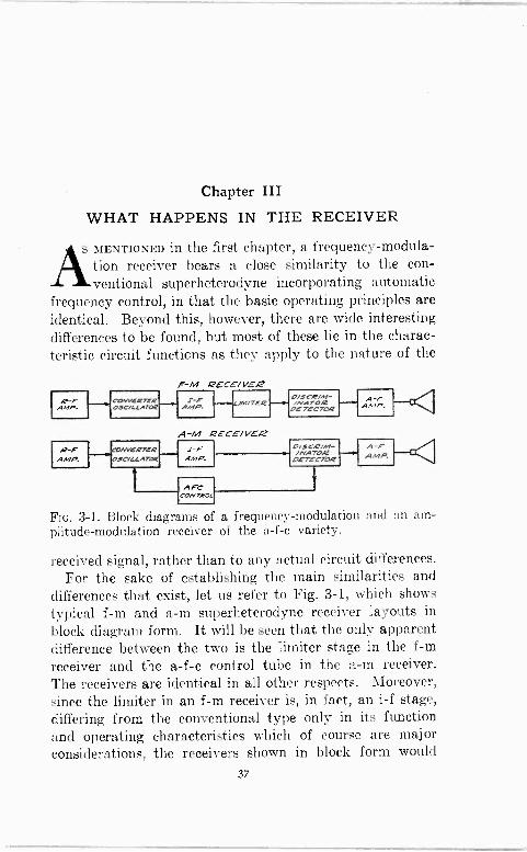
WHAT HAPPENS IN THE RECEIVER
-, MENTIONED in the first chapter, a frequency -modula- tion receiver bears a close similarity to the con- con-
ventional superheterodyne incorporating automatic frequency control, in that the basic operating principles are identical. Beyond this, however, there are wide interesting differences to be found, but most of these lie in the charac- teristic circuit functions as they apply to the nature of the
Q -F .1MP.
F --M QECE/VEQ CAVY£RTtR E -F O/SCR/M- 09C/GC.TQQ - AMP. /TGR -.-e./NA TOR
OETECTOR
A -M RECE/ vea NERTER I -F
9C/GLATO. AMP.
AFC CONTROL
O/SCP/,- /NATO,2
oETECTCz
Flo. 3-1. Block diagrams of a frequency -modulation and an am- plitude -modulation receiver of the a -f -c variety.
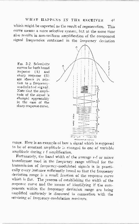
received signal, rather than to any actual circuit differences. For the sake of establishing the main similarities and
differences that exist, let us refer to Fig. 3-1, which shows typical f -m and a -m superheterodyne receiver layouts in
block diagram form. It will be seen that the only apparent difference between the two is the limiter stage in the f -m receiver and the a -f -c control tube in the a -m receiver. The receivers are identical in all other respects. Moreover, since the limiter in an f -m receiver is, in fact, an i -f stage, differing from the conventional type only in its function and operating characteristics which of course are major considerations, the receivers shown in block form would
37
38 FREQUENCY MODULATION
appear similar at first glance if they were drawn in sche- matic form, with the exception that the f -m receiver would have one more i -f stage than the a -m receiver.
Function of R -F Tuned Circuits in F -M Receivers The general function of the antenna and r -f circuits used
in f -m receivers is similar to that in conventional broadcast and short-wave receivers using amplitude modulation. As
in any superheterodyne receiver, the primary function of
these circuits is to select and amplify the desired signal and to reject all other signals. Thus the r -f circuits must atten- uate interfering signals on adjacent channels and at the same time must reduce the image response to which all superheterodyne receivers are subject. In addition, the selectivity of the r -f circuits helps to prevent signals within the i -f range of the receiver from getting into the i -f ampli- fier. This latter function, however, is only an incidental advantage of using r -f tuned circuits, since the suppression of i -f interference can be accomplished directly by means of
an i -f trap. A feature of r -f circuits used in f -m receivers is the pro-
vision usually made in the input circuit for coupling to a
balanced low -impedance transmission line such as is used at the high frequencies allocated to f -m transmissions. Usually, a low -impedance primary winding is used, the center -tap of which is grounded so as to make balanced operation possible. In some cases the center -tap on the primary winding is not returned directly to ground, but is
returned to ground through a wavetrap consisting of a series
coil -and -condenser arrangement. This arrangement has the advantage that a signal voltage is developed across this combination on the regular broadcast and short-wave bands. On these bands the transmission line is no longer balanced, but functions to pick up the signal and apply it to the input circuit. This enables the use of the same antenna for the broadcast and short-wave bands as well as the f -m band. The signal picked up by the transmission line on the f -m band does not reach the grid of the r -f input tube because
WHAT HAPPENS IN THE RECEIVER 39
the circuit is ballanced and the capacitance between the pri- mary and secondary windings of the input transformer is negligible.
Aside from the advantage of the r -f tuned circuits in minimizing interference and image response, the use of an r -f stage has the desirable effect of increasing the overall gain of the receiver and providing a higher signal-to-noise ratio. This reduction in noise level is achieved because a
tube used as an r -f amplifier has a lower inherent noise level than the same tube operated as a mixer tube. Thus the effectiveness of an r -f stage in reducing noise is due to the fact that the gain of the r -f stage is sufficiently great to make the signal ride above the noise level of the converter stage.
Carrier Frequency Amplification Being interested in the frequency -modulation type of
receiver, let us disregard the amplitude -modulation type of receiver and consider the various functions to be found in the former. Perhaps you might be prone to dismiss those circuits which operate upon the carrier frequency with the mere statement that their function is to amplify the signal at a constant level and let it go at that. Yet it is not right to do so, because some very interesting features are associ- ated with the r -f and i -f amplifying systems.
It is simple to say that we amplify at a constant level on the grounds that such a constant amplitude signal of vary- ing frequency is transmitted from the station. But if you investigate closely you will find that while the station trans- mits such a signal, this type of signal is not necessarily received at the receiver and further, amplification through- out the receiver is not always with a constant amplitude signal. In the first place noise impulses will tend to change the amplitude of the frequency -modulated carrier and while it is true that one of the functions to be found in the receiver is the elimination of such amplitude variations due to noise, it is necessary to recognize that such noise is
present until it is removed because it means a better under-
40 FREQUENCY MODULATION
standing of the workings of the receiver. However for the moment we will forget about amplitude variations due to noise and consider the process of amplification of the re- ceived constant amplitude frequency -modulated wave.
What condition exists in the r -f system of the receiver? We know that the r -f and mixer circuits operating upon the carrier are usually tuned to some frequency within the 40 to 44 -mc range; at least such is the case today. The 29 -mc band allocated to the frequency -modulation form of trans- mission is not being used and if there will be any changes in operating frequencies, the direction of travel will be up- wards, so that what we will say will apply.
We know that the frequency -modulated carrier is com- posed of what is the rated carrier frequency with sidebands equal to the maximum frequency deviation. Since much transmission goes on with 100 -percent modulation and since this is equivalent to a frequency deviation of 75 kc each side of the carrier, we can say that the extent of the side - bands is 75 kc each side. Now, as far as the transmission of these sidebands is concerned, they represent audio level, and any suppression of the sidebands means not the loss of certain audio tones, as -in amplitude modulation, but a change in the audio level. Actually this means a change in the relative amplitudes of the frequencies which comprise the audio signal. This as you can readily appreciate is amplitude distortion and is discussed in detail in connection with i -f amplifiers.
When the r -f or mixer section of a frequency -modulated receiver does not pass the full frequency deviation uni- formly, all the frequencies transmitted are present in the received signal, but not in correct amplitude relation. In this case, by correct we mean as transmitted. This is shown in Fig. 3-2. Here in Curve A we show carrier -frequency deviation in terms of amplitude for a number of different audio frequencies, when the r -f system has a sufficiently broad response curve so that all the carrier frequencies contained in the frequency deviation range are uniformly amplified. In Fig. 3-2 B we show a possible response curve
WHAT HAPPENS IN THE RECEIVER 41
which might be expected as the result of regeneration. This curve means a more selective system, but at the same time also results in non -uniform amplification of the component signal frequencies contained in the frequency deviation
FIG. 3-2. Selectivity curves for both broad response (A) and sharp response (B) are shown in rela- tion to a frequency - modulated signal. Note that the ampli- tude of the signal is
changed appreciably in the case of the sharp response curve.
Aºeo c cr aevinriyv range. Here is an example of how a signal which is supposed to be of constant amplitude is changed to one of variable amplitude during r -f amplification.
Fortunately, the band width of the average r -f or mixer transformer used in the frequency range utilized for the transmission of frequency -modulated signals is in practi- cally every instance sufficiently broad so that the frequency deviation range is a small fraction of the response curve which is flat. The process of establishing the width of the response curve and the means of identifying if the com- ponents within the frequency deviation range are being amplified uniformly is discussed in connection with the servicing of frequency -modulation receivers.
42 FREQUENCY MODULATION
It is possible that the reference to amplification at a con- stant amplitude might be confusing in that when we con- sider the process of amplification we always imagine a
varying voltage at the control grid of the tube. This vary- ing voltage exists even during the so-called constant ampli- tude state, because while we speak of constant amplitude, we are referring to the peaks of the individual cycles. All the amplitude peaks are alike, but speaking in terms of instantaneous operation, the signal received from the f -m transmitter is always varying, because as you know the individual cycles of the carrier signal pass through certain instantaneous changes in amplitude. Thus if the carrier is rated at 43 megacycles and is unmodulated, 43,000,000 individual cycles occur in a second and each of these cycles passes through all of its amplitude variations. It is these instantaneous amplitude variations of each carrier cycle which causes the varying potential upon the control grid and the varying current in the plate circuit of the amplify- ing tube. This condition is identical when we amplify an unmodulated or modulated carrier from either an a -m or an f -m transmitter. The reference to constant amplitude in the case of the f -m transmitter is that the peaks of each carrier cycle are the same even when the carrier frequency is changed. Thus if A in Fig. 3-3 is a three-dimensional drawing of amplitude and frequency deviation for an f -m wave and this wave is passed through an r -f amplifying
FIG. 3-3. When an f -m signal is amplified, all the component fre-
_ quencies are am- plified as is in- dicated in the three-dimension- al drawings.
ions are represented in B of the level has been increased but the
the entire signal. However, con - level, the frequency deviation or
FÓ Evi.uT ON~ A)
TIME - vEv;..rá.v
FI
stage, the correct tondit same figure. The signal increase is the same for trary to the increase in
(B)
TIME
WHAT HAPPENS IN THE RECEIVER 43
shift has not been changed. Raising the signal level 10 times or 100 times does not in any way alter the extent of the frequency deviation.
In case you might have in mind the general form of resonance curve and find it difficult to reconcile how it is possible to get uniform amplification of a frequency -modu- lated carrier in a typical r -f stage, we show in Fig. 3-4, a typical resonance curve for the r -f stage in an f -m receiver and at the same time illustrate the portion of this curve (dash lines) which embraces the band -width covered by
Fm. 3-4. Only a relatively small part of the response curve of an r -f stage is taken up by an f -m signal, so that uniform amplifica- tion is obtained.
40 4/ /4L 44 /00 KC .// /00 KC WIDE W/06
FREQUENCY
the f -m signal. You can see the justification for saying that all of the component frequencies represented in the wave are amplified in like manner and that the amplitude of the wave after amplification is pretty much constant. The slight bulge at the top of the resonance curve, which might be construed as representing non -uniform amplica- tion, can be neglected.
Typical R -F Circuits At the inception of f -m broadcasting, that is, when the
first commercial receivers were announced, it was custom- ary to provide a separate r -f channel for operation at the f -m frequencies, but more recent developments have changed the arrangement. The r -f tube used with the f -m transformer is also employed for operation on the regular a -m frequency channels. Switching from one band to the other is accomplished by the conventional methods in use
44 FREQUENCY MODULATION
for years in a -m type receivers, hence no special comments are required. Circuit structure of the r -f stage likewise is
M.
A
C-80 350MMF
111111 pU$N BOTTON 'III? TII? I SNTLN
C-
a
CI6 500MMF
R -q p,00a
R-6 .1 MEC.
FIG. 3-5. R -F and mixer circuit in the Stromberg - Carlson 455 Series.
Courtesy of Stromberg -Carlson.
Fio. 3-6. R -F and mixer circuit in the Stromberg - Carlson 480 Series.
of conventional character and the tubes used are of the type which have been in common use in a -m receivers. A few examples of r -f and mixer input circuit structure as
WHAT HAPPENS IN THE RECEIVER 45
used in some of the commercial f -m receivers, are given in Figs. 3-5, 3-6, and 3-7. We include the mixer input cir- cuits because like the r -f stages, they do not entail radical variations from existing practice.... Of course, the com- ments made in connection with these r -f and mixer stages
13
CM C20 C21 C22 C23 CN C71 C72
sO ee áeee 6SK7
C12
Courtesy of General Electric Co.
FIG. 3-7. R -F and mixer circuit of General Electric Model HM -136.
should not be construed as in any way belittling the devel- opment of f -m reception, that is, the fact that we call the circuit structure of conventional variety.
The Stromberg -Carlson Model 455 series makes use of the more recent arrangement of a single channel for both f -m and a -m reception wherein the transformers are
46 FREQUENCY MODULATION
switched and wherein one tube is used for the r -f amplifica- tion of all signals. The a -v -c circuit arrangement shown is conventional. In the Stromberg -Carlson model 480 re- ceiver, shown in Fig. 3-6, separate channels are used for f -m and a -m, each being a complete r -f amplifier, feeding a mixer and then the i -f system. The General Electric receiver in Fig. 3-7 is of the same character as the S -C model 455. The chassis used in the G.E. models HM -80 and IIM-85 is a straight f -m receiver and is shown in Fig. 3-8. The r -f stage is absent in this receiver. The antenna transformer feeds the mixer. The inclusion of just these two commercial brands is occasioned by the fact that at
6K8 CONVERTOR
C-32 R-7
FIG. 3-8. R -F and mixer circuit in the General Electric Models HM -80, 85.
Courtesy of General Electric Co.
the time of this writing, these schematics are available. Other manufacturers have announced receivers, but data are not available at the moment.
Because f -m receivers at the present time are required to cover only a comparatively narrow range of frequencies, 40 to 44 mc, the design of r -f stages is simplified consider-
WHAT HAPPENS IN THE RECEIVER 47
ably. The comparatively small range over which the re- ceiver must be tuned not only makes it possible to use smaller values of capacitance across the tuned circuit so that a higher L -C ratio and higher gain can be obtained, but at the same time it makes it possible to obtain better tracking between the r -f and detector tuned circuits. Usually oscillator adjustments are provided at both the high- and low -frequency ends of the band, while the r -f tuned circuits are adjusted to track near the high -frequency end of the band. In some cases only one adjustment is provided in the oscillator circuit; this adjustment is usually made at the high -frequency end of the band. Since the band is small in comparison with the middle frequency, it is possible to obtain unusually good tracking between the antenna and mixer tuned circuits.
The Mixer and Oscillator Systems As in the case of the r -f stage, very little can be said
about the mixer stage and the oscillator in an f -m receiver because the operation of this portion of the circuit is not altered by the fact that the receiver is used to receive f -m signals. This is evidenced by the mixer systems shown in Figs. 3-5 to 3-8 inclusive. They are like those to be found in the conventional superheterodyne receiver.*
The same is true of the oscillator in the receiver. The f -m receiver essentially is a superheterodyne and as such the general details apply. The fact that the signal varies in frequency does not in any way change the operating characteristics of the heterodyning oscillator. This still is used as a source of a steady heterodyning signal voltage which beats against the varying frequency received input signal and produces in the output circuit of the mixer a varying frequency i -f signal. All of the usual qualifications of a heterodyning oscillator in a superheterodyne apply to the system when used in an f -m receiver.
* For a detailed discussion of the operation of the mixer system, varieties of circuits, etc., we suggest to the person interested, "Serv- icing Superheterodynes," by John F. Rider.
48 FREQUENCY MODULATION
The I -F System Once more we find a situation like that prevailing in the
r -f portion of the receiver: similar circuit structure and function. However, there are two dissimilarities. One is the use of what is known as a "limiter" stage in the i -f system and the other is a condition associated with the constant -amplitude signal. Of these two considerations,
FIG. 3-9. 1st and 2nd i -f stages in the Gen- eral Electric Model HM -136.
Courtesy of General Electric Co.
we will hold the limiter in abeyance until later in this chap- ter and discuss now the operating characteristics of the i -f amplifier up to but not including the limiter stage. This stage is located between the last so-called i -f tube and the discriminator, although in reality the limiter stage is also an i -f stage.
If you examine the schematics, Figs. 3-9 and 3-10, of some of the i -f systems used in commercial frequency -mod- ulation receivers you will see that the schematic representa- tions of the i -f transformers and, for that matter the circuits, are pretty much like the conventional. In some instances, proper coupling is aided by the use of loading resistors in order to ,e cure the proper band width.
As in the case of the r -f systems, these i -f amplifiers are
WHAT HAPPENS IN THE RECEIVER 49
made with various circuit arrangements. In some systems, like Fig. 3-9, the i -f transformers for each stage are con- nected in series, one set being used for the amplification of amplitude -modulated signals at what we now can call some low intermediate -frequency peak, and the other set being used at the i -f peak required for the amplification of the f -m signal.
Courtesy of Stromberg -Carlson
FIG. 3-10. Partial schematic of the i -f amplifier in the Stromberg - Carlson 455 Series.
As you can see the same i -f amplifier functions for both. The fact that the low i -f peak transformers are in series with the high i -f windings does not interfere with the opera- tion at the higher peak. Since each of the transformer windings is a parallel resonant circuit, it presents virtually a short circuit to the passage of the other intermediate - frequency signal. Thus the i -f winding resonated to 2.1 mc, will pass the 455-kc currents without in any way inter- fering with the operation of the i -f amplifier at 455 kc. The same is true as far as the 455-kc winding is concerned at 2.1 mc.
In Fig. 3-10, the first i -f transformer primaries are switched into the circuit when the receiver is shifted from f -m to a -m reception.
5o FREQUENCY MODULATION Of interest in Fig. 3-10 is the use of a combination a -m
and f -m stage for the first i -f amplifier, the output of this amplifier being fed to the demodulator for a -m reception. The a -m transformer primary is in series with the f -m transformer primary and the f -m transformer secondary is separate, feeding into the second f -m i -f stage tube. In other receivers of the combination f -m and a -m variety, a distinctly separate and complete channel is used for the i -f amplifier.
As to the number of i -f stages, it is customary to employ three stages, of which the limiter is one. In view of the high signal level required at the limiter and the use of
Cour eay of Stromberg -Carlson
FIG. 3-10a. The 3rd i -f stage, limiter, and discriminator used in the Stromberg -Carlson 480 Series. Note that di- rect capacitive coupling is used in the i -f transformers.
one or possibly no r -f stage and the fact that the gain per stage of r -f and i -f is low at the high frequencies in- volved, a greater number of i -f stages are used in such f -m receivers than in the a -m type of receiver. In this connec- tion, the presence of the limiter and its signal requirements also calls for a high gain i -f system.
Amplification in I -F Stages Of interest is the statement that the signal being ampli-
fied in the i -f amplifier is of constant amplitude at all fre- quencies in the deviation band. Any discussion to the con- trary is not with the intention of contradicting the basic underlying principles of f -m operation, but rather as a dis-
WHAT HAPPENS IN THE RECEIVER 51
cussion of the conditions which exist in certain portions of the i -f amplifier and how these conditions are corrected.
Let us for the moment assume that a constant amplitude signal is available from the plate circuit of the mixer tube. Will this constant amplitude signal be available in the f -m i -f amplifier? Judging by what we know to be the character- istics of i -f transformers, the answer is in the negative. Such actually is the case. If we consider the i -f system between the mixer tube plate and the input of the limiter tube as a whole, the overall frequency response of this
FIG. 3-11. The response curve of an i -f ampli- fier, showing that all the frequencies within the deviation range do not N
receive the same amount of amplification.
fLEQUENCY
--B
system resembles a curve similar to that shown in Fig. 3-11, where fo is the i -f peak and fl and 12 are the lower and upper limits respectively, about 100 to 125 kc each side of the peak. Obviously the peak of the response curve above the dotted line A -B would never be called flat-topped and since this peak represents response or amplification at various frequencies, it is easy to see that if a signal of constant amplitude over a frequency range of 75 kc each side of fo is fed into the circuit from the mixer tube, the voltage at the input of the limiter will have variable ampli- tude at the different frequencies within the frequency devia- tion range of the signal. Some frequencies, namely those representing the lowest audio amplitude or minimum fre- quency deviation, will be amplified more than those rep- resenting the louder signals which cause the greatest frequency deviation.
Let us for the moment assume that the relationship be- tween amplitude and frequency deviation for the f -m signal in the mixer tube is like Fig. 3-12, wherein the 2.075 -mc and the 2.125 -mc signals represent 10,000 -cycle audio tones
52 FREQUENCY MODULATION
of a certain amplitude and the 2.175 -mc and the 2.025 -me signals represent a 200 -cycle tone of greatest amplitude. If this is passed through an i -f amplifier or transformer with a response or resonance characteristic like Fig. 3-13, the
FIG. 3-12, left. Fig. 3-13, right. These figures illus- trate the effect of non -uni- form amplification, which is explained in the text.
relationship between amplitude and the component fre- quencies in the circuit is like that shown.
In this exaggerated case, the signal level of the 2.025 -me and 2.175 -mc signals is less than before, but they are never- theless present, whereas the signal level of the 2.075 -mc and the 2.125 -mc signals is greater than before. The fact that the level of the various component frequencies has been increased has in no way altered the number of different instantaneous frequencies present in the i -f signal. You will see later that all of these variations in amplitude are ironed out and that one primary amplitude consideration is that once the leveling action has taken place, all of the component frequencies present in the signal be of the same amplitude. Variations in amplitude are productive of dis- tortion. Just why this is so will become evident later in this chapter.
Having discussed these details associated with the reson- ance characteristics of the i -f system, we again find it fortunate to be able to say that such amplitude variations have no effect because of the operating principles of the system. However, the facts given with respect to the resonance characteristics of such i -f systems are neverthe- less of importance in connection with maintenance because the types of defects which might develop in such a receiver are myriad and it is well to be able to interpret observa- tions made during service work.
WHAT HAPPENS IN THE RECEIVER 53
That the commonplace type of selectivity curve will pre- vail in i -f amplifiers used in f -m receivers is natural when viewed from the angle of selectivity. Not only is the i -f amplifier called upon to magnify the desired signal to its required level, but it must do its share in the elimination of interfering signals. Therefore it must have certain re- jecting powers and these are obtained by resonating the circuits so that they respond over a certain predetermined frequency range.
Furthermore, while it is true that the limiter, to be dis- cussed later, tends to eliminate noise by eliminating ampli- tude variations, the power of selectivity possessed by the i -f amplifier resonant circuits contributes to the minimiza- tion of noise. There are several other considerations asso- ciated with the i -f amplifier, but these will be discussed when we speak about the limiter, the discriminator and the subject of servicing.
The Limiter Stage The final i -f stage in an f -m receiver is known as the "lim-
iter" and differs slightly in circuit arrangement from the preceding i -f amplifying stages, as may be seen in Fig. 3-14.
FIG. 3-14. Schematic of a typical limiter circuit. Note the low plate and screen voltage.
Although employed for a special purpose, the stage provides a certain amount of gain over the range of frequency repre- sented by the i -f peak and the maximum frequency devia- tion. The primary function of the tube is to act as an amplifier which is very easily overloaded; that is, grid cur- rent is caused to flow and plate current saturation is pro- duced on one half of the signal cycle and plate current
54 FREQUENCY MODULATION
cutoff is created on the other half of the cycle. The pri- mary purpose of the tube is to wipe out all amplitude variations present in the output of the i -f amplifier system ahead of the limiter and to pass on to the discriminator a constant amplitude -varying frequency signal. In other words, it is a sort of electrical gate, functioning in a manner similar to that shown in Fig. 3-15. At least this is the
I I
I I "d1UiViúI!îvP,
FIG. 3-15. A pictorial representation of the action of the limiter in removing all amplitude variations.
theoretical ideal condition. The deviations from this ideal condition will be discussed later.
The method of creating the required operating state for the limiter is by a combination of conditions. First a sharp cutoff type tube is used, like the 6SJ7, with comparatively low values of screen and plate voltage and little or no initial control grid bias, so that the tube will overload very easily and plate current cutoff is quickly reached. The operating point is established at the center of the linear portion of the plate current -grid voltage curve by the application of the correct operating potentials. Under the proper conditions, signals of comparatively small amplitude will swing the grid voltage into that zone which will cause plate -current cut- off and plate -current saturation, thereby limiting the magni- tude of signal plate -current variations in the plate circuit. Of particular interest is the fact that this tube does not function to or in any way limit the frequency excursions of the modulated i -f signal. It limits the amplitude of the signals in the plate circuit.
This action of the limiter is easily understood from the drawing of Fig. 3-16, which shows one cycle of carrier sig- nal voltage plotted against the grid voltage -plate current
WHAT HAPPENS IN THE RECEIVER 55
curve of the tube. In this figure, A is the point of plate - current cutoff, B the center of the linear portion of the grid voltage -plate current curve; and C the point of plate -cur- rent saturation.
It will be seen that any variations in signal voltage within the limits of BA and BC along the grid -voltage line will result in corresponding variations in the plate current of
FIG. 3-16. A sin- gle cycle of car- rier signal ap- plied to the lim- iter stage, show- ing the clipping action on both the positive and negative peaks.
F
tp
e
4
the limiter tube; but no such plate -current variations will result from variations in signal voltage beyond points A and C where cutoff and saturation are reached. In other words the instantaneous signal peaks EFG and IJK have no effect upon the plate current. Since the operating point is estab- lished at the center of the linear portion of the plate -current curve, both halves of the resulting plate -current cycle will be equal in amplitude, but the current peaks will be flat- tened out by the limiting action, as shown in the figure. In effect, then, the positive and negative signal peaks are clipped off; the resulting plate current consisting only of variations corresponding to the signal -voltage amplitude variations_ lying between DEGHIKL and corresponding to AB and BC on the plate -current curve.
Further analysis of Fig. 3-16 brings a few pertinent points to light. In the first place to get any clipping or limiting action, we must cause a plate current swing or variation, in excess of from B to A and from B to C. If by chance the amplitude of the signal voltage applied to the control grid is such that the swing in plate current is less than BA and BC, then the signal currents in the plate circuit will be
CARR/ER 5/GNAL VOLTAGE
PLATE CURRENT
+ E9
56 FREQUENCY MODULATION
reproductions of the change in amplitude in the grid circuit and the tube will function as a commonplace amplifier in- stead of a limiter. This will defeat the purpose of the tube and impair the attainment of the advantages which accrue from the clipping or limiting action. All of this means that for proper operation of the limiter tube, a prescribed mini- mum signal level must prevail at the control grid.
Further examination of the curves of Fig. 3-16 must, ih
accordance with amplification processes prevailing in a -m type systems, lead to the momentary conclusion that such action of the limiter tube results in the development of dis- tortion in the plate circuit. After all, we are accustomed to plate -current variations which are enlarged reproductions of grid -voltage variations. The distortion prevails, but it is of no consequence because when we clip the amplitude of the wave, we are not changing the relative frequencies present in the frequency deviation. You might recall that earlier in this chapter we increased the amplitude of the wave but did not change the component frequencies. In other words an instantaneous frequency of 2.175 me does not undergo any change if it is increased from 10 volts to 50 volts or reduced from 50 volts to 30 volts. And even if the clipping action does introduce harmonics, they are of no importance because the frequencies representing these harmonics do not appear across the resonant circuit located in the plate circuit of the limiter. This circuit responds only to the range of frequen- cies representing the frequency deviation both sides of the carrier, and perhaps a little beyond these limits. The har- monic frequencies are filtered out of the circuit by the trans- former which couples the limiter to the discriminator.
Now let us consider in Fig. 3-17 this limiting action in connection with a frequency -modulated wave which has been passed through the i -f amplifiers ahead of the limiter and the various component frequencies were unevenly am- plified. Those closest to the carrier i -f frequency with mini- mum frequency deviation were amplified most and those with the greatest deviation amplified the least. This con- forms with the information to be gathered in previous dis-
WHAT HAPPENS IN THE RECEIVER 57
cussions concerning the response curves of i -f amplifier stages. The height of the peaks from the signal voltage zero line indicates the amplitude of the component frequencies in the wave. These component frequencies in the signal wave are identified in terms of frequency deviation. It should be understood that while only a few cycles of input signal voltage are shown as being representative of a frequency deviation from 0 to 75 kc, a great number of such cycles exists in the actual wave.
E
v Y
ñ ? O
L /.M/TEQ. OUTPU>
]S C - 40
S
f -- 75 K C
A' O C' /NPUT -5/GA/AL AMPL/TUDE
/0 FREQUENCY O
OEV/AT/ON OF /NPUT .J/6NAL.
/O
ao FIG. 3-17. The output of the limiter remains constant regardless of variations in amplitude at the grid.
We note in Fig. 3-17, that the lowest signal voltage am- plitude is sufficiently great to swing the plate -current into the cutoff zone on the negative cycles and into the plate - current saturation zone on the positive cycles. This is shown by an extension of the two limits A and C of the plate cur- rent swing between the cutoff point and the point of satura- tion, namely lines AA' and CC' through the representations of the signal voltage. All of the signal voltage peaks to the left of the line AA' and to the right of the line CC' have no effect upon the plate current, the former because these peaks change the grid voltage after the tube has reached plate - current cutoff and the latter because the peaks occur after the tube has reached the plate -current saturation point.
58 FREQUENCY MODULATION
If we now plot the plate -current variation for these signal voltage cycles, we find that the plate -current variations rep- resenting currents of different frequency, identified by the deviation figures, are of uniform amplitude.
Now let us consider this limiting action in relation to an f -m signal upon which is superimposed a number of noise peaks, as shown in Fig. 3-18. As you can see the wave is
IP-.. C --T - -ter
E9
SIGNAL ANO NO/5E OLTA6E
1 PLATE CURRENT OUTPUT
FIG. 3-18. The ac- tion of the limiter in removing noise pulses so that the
- discriminator out- put will not be ef- fected.
A' C'
non -uniformly amplified and further variations in ampli- tude are produced by noise peaks which have combined with the wave and still further change its amplitude. Of course these noise components are of varied magnitude and those which have an amplitude much less than the signal voltage are over -ridden by the signal, but those which are stronger than the signal, would under normal conditions be repro- duced. But it is seen that, by virtue of the limiting action, any signal or noise voltage in excess of that required to drive the grid of the tube to plate -current cutoff in the nega- tive region and to plate -current saturation in the positive region, will not cause corresponding changes in the plate current. Therefore the signal and noise peaks to the left of the dotted line AA' and to the right of the dotted line CC' are effectively wiped out of the output signal, which, though it corresponds in frequency to the input signal, does not vary in amplitude.
WHAT HAPPENS IN THE RECEIVER 59
It should be observed from Fig. 3-18 that the limiter behaves like an ave system. That is, the output signal re- mains practically constant for any increase in the amplitude of the input signal above that required for limiting action. Therefore, the output of the limiter is substantially inde- pendent of input, and the signal voltage fed to the discrimi- nator -detector will be of constant amplitude for all signal voltages above the limiting threshold.
Varying Sensitivity of Limiter The actual signal level in the output circuit of the limiter
is governed by the possible relative changes in plate current that can take place between points A and C. This output level' can be raised or reduced by increasing or decreasing the operating voltages on the tube. In reference to Fig. 3-18, the effect of increasing the values of plate and screen voltage would be the equivalent of moving out the points of plate - current cutoff and saturation, A and C, and therefore in- creasing the spread between the threshold limits AA' and CC'. This would call for a signal of greater amplitude to produce the limiting action, but it would also result in a correspondingly larger signal output, and consequently less audio gain following the discriminator -detector would be needed. On the other hand, if the limiter -tube operating voltages were reduced, the cutoff and saturation points A and C would be brought closer together, and the spread between AA' and CC' would be reduced. In this case a sig- nal voltage of much less amplitude would suffice to produce the limiting action, and less gain would be required in the r -f and i -f stages. But the signal output of the limiter would be correspondingly reduced, calling for higher audio gain following the discriminator -detector.
It would appear from the foregoing that the most appro- priate operating point for the limiter would be that which called for the least signal input voltage. Yet this would contradict an earlier statement that an r -f signal of consid- erably large amplitude is required for the proper function- ing of the limiter tube. The reason for this is that first,
60 FREQUENCY MODULATION
proper limiter action must take place over the full frequency deviation range and, as you will see later, there is a marked difference between the signal level at the i -f peak and at the limits of the frequency deviation range. Secondly, the substantially flat points of cutoff and saturation that can be reached are considerably beyond the point where limiting action first takes hold. As a typical example, the tube may start to limit with a signal input in the neighborhood of 3 volts, level off at 5 volts, but not become substantially flat at a signal input of much less than 12-14 volts.
The full implication of this characteristic of the limiter will be appreciated by reference to Fig. 3-19 where the grid
--7.--.7."" ==r_ r_ ,
-T/
.
/NPV7 S/GNAL AMPO/7V06
r PLATE CuaREN7 VTPVT
Fm. 3-19. The action of the limiter circuit for strong and weak signals.
voltage -plate current curve more closely approximates the actual. For the sake of the discussion, we have shown the r -f input signal with a gradually ascending amplitude and noise peaks with random amplitude. As before, AA' and CC' represent the points at which limiting action is fairly complete.
Now, it will be seen that from point .1 to point 2 the sig- nal amplitude is not sufficient to produce any major limiting action. As a result of this, the noise peaks existing between these points are reproduced in the output signal, the only improvement at all being that those noise peaks having amplitudes sufficient to produce limiting action have been
WHAT HAPPENS IN THE RECEIVER 61
partially clipped. From point 2 to point 3, however, the amplitude of the signal input approaches the value within the limiting action range, with the result that beyond 3 the noise and signal peaks are clipped. But note that the noise peaks between 2 and 3 appear in the output signal, though considerably reduced. The reason for their appearance is due to the fact that the upper end of the plate -current curve beyond C is not completely flat, but continues to rise slightly from point C to point D. Since the noise peak swings the grid into this region and the signal does not, the noise peak produces an additional rise in the plate current which appears in the output signal.
But, from 3 to 4, the input signal is of such amplitude that it swings the grid beyond point D and into that region where the plate current levels off. In this case, the high - amplitude nóise peak existing between 3 and 4 swings the grid still further into the positive region, but, since the sig- nal has established the operating point on the substantially level portion of the plate -current curve beyond D, the more extensive swing in grid voltage due to the noise peak merely moves the operating point further along on a curve that is flat. Hence there is no change in plate current correspond- ing to the instantaneous noise peak, thus the noise pulse is eliminated from the output.
Signal Input vs Signal Output at the Limiter We have shown a few illustrations of how the action of
the limiter tends to overcome variations in signal amplitude developed in the i -f amplifier as a result of the non -uniform selectivity characteristics of the various i -f amplifier stages. All of these facts were presented in connection with the grid voltage -plate current characteristic. In Fig. 3-20, we show the manner in which the output of the limiter varies with the input. The facts conveyed in this figure can easily be reconciled with the information shown in Fig. 3-19.
An examination of Fig. 3-20 and a comparison of curves A and B, shows that the limiter output signal (curve B) is dependent upon the limiter input signal (curve A) over a
62 FREQUENCY MODULATION
certain zone of operation. These curves are actually meas- ured curves for a commercial f -m receiver. From the start of each curve until points X and Y respectively are reached, an increase in signal input is accompanied by an increase in signal output, so that the limiter tube is acting like a con- ventional amplifier tube. The degree of amplification can be established by comparing the levels of the input and output signals in accordance with the designations shown upon the vertical axis. The input signals to the antenna corresponding to various input and output signals at the limiter are shown upon the horizontal axis and are quoted purely for illustrative purposes. While the figures given apply to the specific receiver in question, they should not be accepted as being specific values applicable to all f -m re- ceivers. You can readily understand that these carrier sig- nal levels at the antenna indicate sensitivity of the receiver and it stands to reason that sensitivity is not standard in all receivers.
As is evident in Fig. 3-20, the limiting action just about starts at X on curve B and as you can see this means an input signal voltage to the limiter of about 2 volts and an input signal at the antenna of about 40 microvolts. The output signal voltage from the limiter is approximately 4.4 volts. Further increases in signal input to the limiter, caused by further increases in the signal input to the an- tenna do not cause corresponding increases in the limiter output, although it is true that an increase in signal output is obtained.
Continuing along curve A, the signal input to the limiter, we find that a point is reached, Z, when the signal input and signal output are the same. In other words the action of the limiter tube as an amplifier ceases and this condition pre- vails for a signal input at the antenna of about 100 micro- volts. As you can readily understand, this condition of unity amplification in the limiter tube need not occur with a 100 microvolt input in all receivers. The ave system is an influence, in that the faster the action of the ave voltage, that is the greater the avc voltage for small values of signal
WHAT HAPPENS iN THE RECEIVER 63
input at the antenna, the greater will be the required signal input to create unity amplification in the limiter. In this connection the magnitude of amplification prevailing ahead of the limiter is also a factor, in that the greater the ampli- fication per stage, the less will be the required signal input at the antenna to cause a balance between signal input and signal output at the converter.
2
0
LIM TEQ ACT/ON
ccv< A-J/6NAL rOerAee Ar c/787212 eºw cuavE ®-mcNm 207303 rc,,,,,z,,,,,,yr
I / y,
CURVE
CURVE Ci X X' - Y _-- --' . __ ____ .,.... .,,,,,.
TO 30 90 BO 70 mtcgovocrs INPUT SIGNAL TO RECE/VER
000
FIG. 3-20. Curve A shows the signal voltage at the limiter grid while B shows the voltage at the limiter plate for different values of input signal. Note the leveling action in B.
Advancing beyond point Z in Fig. 3-20, we note that the limiter tube is no longer acting as an amplifier. Of course it is still an operating tube, but instead of amplifying the signal, just the reverse is true; the output signal is less than the input signal. However, to be accurate, we must state that the output is not absolutely fiat for increases in signal input beyond the point Z. A very slight increase in signal output for an increase in signal input still exists, but for all practical purposes, we can say that the limiting action has about reached a state of stability. Points X' and Y' indi- cate the levels beyond which an increase in signal input creates but a very small change in signal output. In fact increasing the signal input at the antenna to approximately 50,000 microvolts caused an extremely small increase in signal output above that prevailing at X', when the signal input was Y' equal to about 12 volts at the limiter and 600
64 FREQUENCY MODULATION
microvolts at the antenna. The departure from the steeply climbing curve A between Y and Z, beyond Z is due to the action of the avc.
A few interesting observations can be made in connection with Fig. 3-20, but in order to make them, we must intro- duce another condition, namely the selectivity characteris- tics of the i -f amplifier. Once again the curve shown in Fig. 3-21 applies specifically to the receiver in question, but it is possible to say that a similar curve will be found to apply to the majority of f -m receivers, because such selec- tivity characteristics are typical of the majority cf i -f am- plifiers unless special band-pass coupling systems are incor- porated. Such special circuits are not to be found in the usual run of f -m receivers, primarily because they are not essential to the proper operation of the circuit. After hav- ing discussed Fig. 3-21, we will correlate the data with those shown in Fig. 3-20.
Selectivity Characteristics of I -F Amplifier There is a definite relation between the required signal
input to an f -m receiver, the operation of the limiter and the selectivity characteristics of the i -f amplifier preceding the limiter. We know that the function of the limiter is to provide a constant level signal for application to the dis- criminator. Fig. 3-20 shows that the limiter is capable of accomplishing this. However we must also recognize that the signal being fed into the limiter is not of constant ampli- tude; that if proper limiter action is obtained upon the peak frequency of the i -f amplifier, the required signal will not necessarily be available at various frequencies within the deviation range.
This is shown in Fig. 3-21, wherein the signal level at various frequencies within the deviation range is compared with the signal level prevailing at the peak frequency. This curve is made without the avc acting and at a signal input to the receiver of 40 microvolts. While it is true that the curve will undergo a few minor variations at greater input signal levels because of the action of the limiter tube upon
WHAT HAPPENS IN THE RECEIVER 65
the i -f transformer which feeds that tube, the illustration as shown is still usable for purposes of explanation.
This curve shows in more definite form, some informa- tion conveyed in Fig. 3-17. in that figure we illustrated a variation in signal input level and also that the input volt- age was made up of various frequencies, representing fre- quency deviation of the carrier. Further, the illustration showed that a certain minimum signal input voltage level was required at the greatest frequency deviation range in order that the limiter output be uniform over the entire frequency deviation range
FIG. 3-21. Selectivity characteristic of an f -m receiver discussed in the text. This curve is sharper due to re- generation than is nor- mally preferred in f -m receivers. Modern de- sign of the i -f system calls for the signal at the maximum devia- tion to be down not more than two or three times from the peak.
á 60
60
3
2
Y Y'
x'
.uo /ro ao 80 co 40 ¢o 0 20 40 60 80 /oo zo /40 K/LOCYCLES OFF RESONANCE
This is also shown in Fig. 3-21. The figures shown upon the vertical axis indicate the ratio between the signal volt- age off resonance to that at resonance at the limiter grid. The figures along the horizontal axis indicate the frequency of the signal voltages with, respect to the peak frequency, which is indicated as being 0 kc off resonance. Thus if the peak frequency were 2.1 me a signal indicated as being 30 kc off resonance, would be a frequency of 2.070 me on one side and 2.130 me on the other side.
66 FREQUENCY MODULATION
Referring to Fig. 3-21, we note that the maximum fre- quency deviation of 75 kc encountered in present-day f -m operation is down 10 times with respect to the level at the peak frequency. Being down 10 times means that the level of the signal at that frequency is 1/10 of that prevailing at the peak frequency. For deviation frequencies less than 75 kc, other values prevail, as for example, a signal which is 40 kc off resonance on both sides is down about 2 times, which means that if the i -f peak is 2.1 me and if the i -f amplifier has a selectivity characteristic as shown, a fre- quency deviation of 40 kc will result in a signal at the lim- iter grid which will be 1/2 of that prevailing at the peak frequency.
Now, if we assume that the input and output signal rela- tions shown in Fig. 3-20 were established at the peak fre- quency of the amplifier, (0 kc off resonance in Fig. 3-21) , then in accordance with Fig. 3-21, if we want the signal representing a frequency deviation of 75 kc to have the same magnitude at the limiter grid as the peak frequency signal, this 75-kc off resonance signal must be increased 10
times and the 40-kc off resonance signal must be increased twice. Other off -resonance ratios are indicated in Fig. 3-21.
What does all of this mean? It means first, that recogniz- ing the existence of a constant level frequency -modulated signal at the antenna, the non -uniform amplification exist- ing in the receiver requires that a certain signal level prevail at the antenna in order that the signal voltage at the limiter grid be sufficiently high at all frequencies within the com- plete frequency -deviation range so that limiter action take place over this range of frequencies.... We do not mean to stipulate just what this signal at the antenna must be, be- cause many factors contribute to the establishment of the minimum. Such items as the amplification within the re- ceiver, the arrangement of ave, the existence of delayed ave, the distance between transmitter and receiver, efficiency of
radiation at the transmitter and pickup at the receiver, the operating voltages applied to the limiter, the frequency
WHAT HAPPENS IN THE RECEIVER 67
deviation employed during transmission, etc., all these have their influence.
However, the fact does remain that if the signal voltage at the antenna is of such a level that operation of the limiter takes place only at the peak frequency; or if such condi- tions prevail in the receiver that the peak frequency signal is amplified out of proportion to the other component fre- quencies, the non -uniform amplification which prevails in the i -f system ahead of the limiter will exist there and the output signal voltage curve with respect to frequency will resemble that, of curve A in Fig. 3-22.
4O.4 vOt7 INPUT ..5/ANAL
2. Ou 2./
(a) 2./75
80,,U VO INPUT 5/6NAL f -8O KCB
2.06 2.1 2.140 FPEqUENCY --
400 .1.4.. VOLT INPUT SIGNAL .-/50 KC -
2.423 2./
(b) ' (c) Fla. 3-22. These curves show how limiter action broadens the selectivity for strong signals. (These curves are theoretical.)
If the signal input is such that the signal voltage at the grid of the limiter at the peak frequency and say for a frequency deviation of 40 kc each side of the carrier is of some value exceeding Y in Fig. 3-20, the output of the lim- iter will be substantially flat over a range of 40 kc each side of the carrier, and a representation of the limiter out- put with respect to frequency will be like that shown in Fig. 3-22 curve B.
Curve B is by no means the ideal relationship that should exist at the output of the limiter, but it does indicate a con- dition which might exist and be responsible for a confusing symptom in the receiver. Thus if the transmission from the station is limited to a frequency deviation band of 40 kc
2./75
68 FREQUENCY MODULATION
each sidé of the carrier, a condition productive of the re- sponse curve B in Fig. 3-22, will result in perfect reception, yet that same receiver will show marked distortion if the transmitted frequency deviation band is increased. In other words, if during a single transmission one passage of audio tones is of low amplitude so that the maximum frequency deviation is limited to 40 kc, it will be received without dis- tortion, but if the next passage is loud so that the full allow- able frequency deviation band -width is transmitted, the receiver output will be distorted. Thus what would nor- mally be construed as being overloading is actually the suppression of sidebands, or improper operation of the limi- ter over the required frequency range, due to the fact that. the signal voltage reaching the grid of the limiter is not sufficiently high to cause the tube to operate within the limiting action zone.
The presence of sufficient signal at the antenna so that the signal at the limiter grid over the full deviation range is sufficiently great to cause limiting action produces a re- sponse curve at the limiter output which resembles curve C in Fig. 3-22. Here you can see that the output voltage is substantially level over the full frequency deviation range or over a total band -width of 150 kc. Such a curve develops when, as a result of sufficient signal input, the signal at the limiter would be at least the 2 volts indicated at Y in Fig. 3-20 for the 75-kc off resonance signal.
What is the effect of such flat -topping of the resonance curve by the action of the limiter upon the process of align- ment? At first glance one would be tempted to say that alignment of the individual i -f stage is not of importance inasmuch as the limiter tends to remove the peak. Such however is not the case. While it is true that critical align- ment is not necessary, at the same time haphazard align- ment cannot be employed.
For any one signal input a certain amount of amplifica- tion is required in the receiver ahead of the limiter and this applies equally to the peak frequency and the frequencies within the deviation range. An attempt to stagger the
WHAT HAPPENS IN THE RECEIVER 69
peaks will produce a broader response but it might reduce the amplification sufficiently so that poor results will be ob- tained when the receiver is located at the limits of the trans- mission range or when the signal input is low.
Another possible effect of staggering or incorrect align- ment might be the production of a state equivalent to over - coupling with a dip between two peaks. This in itself might not be bad, even if it reduces the over-all gain, pro- vided that a strong signal is received, because under such conditions the limiter will act over the entire frequency range of the system and the dip in the resonance curve will be of no consequence. However, in the event that the signal input is not as great as it might be, the reduced amplifica- tion due to such staggering might cause the condition that limiter operation will be produced on the peaks both sides of the dip, but not at the frequency representing the loca- tion of the dip in the resonance curve and distortion will result.... This condition is contrary to that produced with a sharp resonance curve which reduces the band width. With the staggered or over -coupled transformers distortion will be more pronounced on weak signals than on strong signals.
Considering all angles, we feel that the action of the limi- ter should in no way influence the alignment procedure. A reasonable amount of accuracy should prevail, even if it is not critical.
Types of Limiter Circuits Very little need be said about the various types of limiter
arrangements that are used in commercial receivers because they are very much alike. The primary difference is to be found in the grid circuit connections. A few typical sche- matic wiring diagrams in Fig. 3-23 illustrate a number of variations. In A, the grid current flows through the coil of the tuned circuit and the ave voltage is developed across the resistor R. In B, the load in the grid -cathode circuit is the combination of resistance R and RI and the direct- current path is isolated from the tuned circuit by the con-
7o FREQUENCY MODULATION
denser C. The ave voltage is that developed across resis- tor Rl. Circuit C is very much like B, except that resistor R shunts the permeability -tuned winding L through the ca- pacity C. The load in the grid -cathode circuit is made up of the combination of R and Rl.
AVC
FIG. 3-23. Representative types of limiter circuits, used in com- mercial f -m receivers.
As far as the plate circuits are concerned, they are pretty much conventional in that these tubes feed into the discrim- inator, and these are substantially the same in most re-
ceivers, as you will see later on in this chapter.
AVC in F -M Receivers Very much need not be said about the use of ave in f -m
receivers. In some instances the conventional arrangements employed for a long time in a -m receivers find use in f -m systems. However, comment is heard to the effect that after further field experience proves the point, the likelihood of elimination of the ave from the f -m receiver is very prob- able. This condition is created as the consequence of an arrangement whereby all or some of the regular i -f tubes are arranged to function as partial limiters. All of the grids are grounded and cathode bias is used. In each of the grid circuits of the i -f tubes a series grid resistor is employed.
In view of the fact that limitation of the amplitude of the i -f signals by partial cutoff in the amplifying tube does not introduce distortion, it is possible to arrange such values of grid bias in these i -f tubes that for signals beyond a certain level at the individual grids of these tubes, overloading takes place with the result that major differences in signal levels are ironed out even before the regular limiter tube is
reached.
WHAT HAPPENS IN THE RECEIVER The Discriminator
The discriminator is not new in the ranks of radio re- ceivers. The automatic -frequency -control systems of a few years ago employed the discriminator as a means of developing a control voltage intended to adjust the oscilla- tor in the receiver automatically so as to produce the correct heterodyning frequency and in that way compensate for any mistuning on the part of the person operating the receiver. In the a -m type of receiver the function of the discrimina- tor was to convert frequency variations into d -c control voltages.*
In the f -m receiver, the basic function of the discrimina- tor is to convert the frequency -modulated i -f carrier into audio -frequency variations of different amplitude. When we say that the discriminator in an f -m receiver converts the frequency -modulated i -f carrier into audio voltages of what- ever amplitudes are represented in the signal, we already embrace the utility of the system as a detector. While it might be possible to identify the system as the discrimina- tor -detector, to give it its full title in accordance with its use, it has become common practice to refer to it as the discriminator and take for granted the detector action.
To ask "What happens in the discriminator?" is only a natural question. The statements made in the preceding paragraph are general and concern the final result. Let us therefore analyze in a general way the manner in which the frequency -modulated signal is converted into an ampli- tude varying audio signal.
Suppose that for the moment you glance at Fig. 3-24. Here we illustrate a form of discriminator circuit which is not exactly Iike that employed in frequency -modulation re- ceivers, but is still suitable for a basic explanation of how a discriminator operates. A tuned circuit Ti secures from the amplifier tube VI, which can be the limiter tube in an f -m receiver, a variable frequency voltage which is constant in amplitude over the frequency deviation range. Let us
* A complete detailed discussion of the discriminator appears in "Automatic Frequency Control Systems," by John F. Rider.
71
72 FREQUENCY MODULATION
assume that the frequency range of this signal is from 1.925 mc to 2.275 mc, roughly a total band width of 350 kc or 175 kc each side of the mean frequency of 2.1 mc. Actually this band width is not employed in practice, but once again, it is being used for the sake of illustration.
The primary winding Tl is coupled to the two tuned cir- cuits T2 and T3, each of which is in turn connected to a
FIG. 3-24. A discrimi- nator circuit in which. two staggered tuned cir- cuits are used to obtain the desired action.
conventional diode rectifier, DI and D2. If you wish you can consider these two diodes in one envelope but we show them separately to simplify the discussion. The two loads upon these two rectifiers are represented by Rl and R2 and, as you can see, these two rectifiers are arranged in what is known as a differential rectifier system. Although each rec- tifier tube has its own load resistance, and the rectified voltage developed in each rectifier is present across the respective load resistances, the two voltages are of opposite polarities and therefore tend to buck or cancel each other. The final or resultant rectified or output voltage present across the series combination of load resistances, or between ground and the point P, depends upon the relative magni- tudes of the individual voltages across Rl and R2.
If the two rectified voltages across Rl and R2 are equal, the net voltage between ground and point P is zero. If that across R,L is greater than that across Rl, the final voltage between ground and point P is equal to that across R2 minus that across Rl. If that across Rl is greater than that across R2, then the final voltage is equal to that across 'RI minus that across R2. As to the polarity of the voltage between ground and point P, that depends upon the polarity of the greater voltage across Rl and R2. The fact that
WHAT HAPPENS IN THE RECEIVER 73
point P and ground bear negative signs does not mean that they are fixed in polarity. These signs are used to indicate the fact that the two load resistances are connected into a differential circuit and the voltages across them tend to buck each other. As far as point P and ground are concerned, either can be positive or negative with respect to the other, depending upon the magnitude of the voltages across Rl and R2.
Now since the two tuned circuits T2 and T3 are peaked to different frequencies, their response to the frequencies present in Ti will be different. If we plot the response of these two circuits in terms of frequency, as in Fig. 3-25, we
JO
40 W 0 30
Q 10
[ io
o /.923 1.975 5.021 1.075 L/ 2./23 5175 2.125 2.275
MC FREQUENCY -
FIG. 3-25. The signal voltage developed across T2 and T3 in the discriminator circuit shown in Fig. 3-24.
MC
note that only at one frequency, namely 2.1 mc, is the re- sponse of both circuits the same. At all other frequencies the response of T2 is different from that of T3, with the result that the magnitude of signal voltage fed to the two rectifiers for rectification depends upon the response of the circuit to the frequency of the signal voltage.
Now the significant detail is that at any one instant, only one frequency exists in the system and whether Di or D2 or both will be rectifying the signal depends entirely upon the frequency of the signal voltage. Thus if at any one instant the frequency of the signal is 2.025 mc, the circuit which responds to this frequency is T3 and rectification will take place in D2 and the rectified voltage will appear across R2. As a matter of fact this is true for all frequencies from 1.925 mc to approximately 2.075 mc. Between 2.075 mc and
74 FREQUENCY MODULATION
2.125 mc, both tubes are operating and the differential volt- age is developed between point P and ground. Between 2.125 mc and 2.275 mc only T2 is responsive and the signal is being rectified in Dl and the rectified voltage appears across Rl.
Recalling that the polarities of the voltages developed across Rl and R2 are different, we then have, in conformity with the condition mentioned in the previous paragraph, a situation wherein voltages positive with respect to ground, which can be the zero reference point, are developed across R2 and voltages negative with respect to ground are de- veloped across Rl.
If we now plot the output voltage across Rl and R2 respectively with respect to frequency, which means the response of T2 and T3 respectively, we secure a graph which
FIG. 3-26. The d -c volt- ages developed across Rl and R2 in the dis- criminator circuit shown in Fig. 3-24.
looks like that shown in Fig. 3-26. The reason that the response of the T3 system is shown above the frequency reference line is that the voltage developed across R2 is positive with respect to ground. The response of the T2 system is shown below the reference line because the voltage developed across Rl is negative with respect to ground.
We now can take these two curves and combine them into the typical "S" characteristic of a discriminator by simply combining the voltages developed across Rl and R2 as shown in Fig. 3-26. For example at the mean frequency of 2.1 mc the response of T2 is the same as that of T3 and the voltage developed across RI is the same as that across R2, but since they are of opposite polarity, they cancel and
WHAT HAPPENS IN THE RECEIVER 75
the net output voltage from the rectifier system is zero as indicated in Fig. 3-27.
Other output points are developed in similar fashion. For example at 2.09 mc greatest response is secured in T3 and according to Fig. 3-26, the rectified voltage across R2 is 6
FIG. 3-27. The overall output of the discrimi- nator circuit shown in Fig. 3-24. The linear por- tion is indicated by X and Y.
W boas t-oo t.Ots t.aas
,amom-nr--
volts, whereas the rectified voltage developed across R1 is 1 volt. Since these two voltages are of opposite polarity, the net final output voltage is 5 volts as shown in Fig. 3-27 and the polarity of this voltage is positive with respect to ground because the greater voltage was developed in the T3 -D2 -R2 system. On the other hand at a frequency of 2.110 mc, which represents the same deviation from the mean of 2.1 mc as the 2.090 mc signal, the final voltage again is 5 volts, but this time negative with respect to ground, because the greatest response to this frequency takes place across T2, hence the greatest rectified voltage is developed in the T2 -D1 -R1 system.
Looking at Fig. 3-27, we can make certain observations which will be of interest later. In the first place here is a rectifying means whereby we can convert frequency varia- tions into audio voltages of different amplitudes. Second, we see a zone of operation wherein a uniform change in frequency results in a linear output; this is over the straight portion of the curve between X and Y. Third, with this straight portion as the basis of a discussion, we can realize that in order to secure a linear output, the frequency ex- cursions should not exceed the linear portion of the dis- criminator characteristic.
76 FREQUENCY MODULATION
It might be well at this time to assume a signal of con- stant amplitude across Tl, and to establish the manner in which the discriminator action produces the variable ampli- tude audio output.
Referring to Fig. 3-28, suppose that we apply to the dis- criminator tube a frequency -modulated signal with a maxi- mum deviation of 50 kc each side of the 2.1 -mc carrier. This is the i -f signal frequency -modulated. We mention the frequency -modulated i -f signal rather than the fre- quency -modulated r -f signal because it is the i -f signal which is applied to the discriminator input. You, of course, realize that in the operation of a superheterodyne receiver, and the f -m receiver is a superheterodyne-the i -f signal retains all of the characteristics of the original r -f signal.
If you now follow out the plotted points in Fig. 3-28, you will note that the output voltage from the discriminator is
zero when the input signal is of the same frequency as the mean of the complete range covered by the discriminator response. The reason for this is explained in connection with Figs. 3-25 and 3-26.
Now the frequency of the input signal is changing and we note that the first deviation is in the positive direction, that is the frequency increases to an extent indicated by A
and is equal to approximately 25 kc. Since the design of the discriminator is such that when the frequency increases and negative voltage is developed in the output, we have a change in output voltage from zero to slightly more than 10 volts and if we show this output voltage with respect to a zero voltage reference line, we reach the peak negative voltage A' in the audio output curve. From A in the input signal curve the frequency deviation decreases and we have a corresponding decrease in the output voltage. Since the change in frequency from the maximum deviation at A
to the mean frequency is still within the plus zone, the output voltage is still negative until it reaches zero. Now the frequency of the input signal is again changing, but this time in the downward direction and the design of the discriminator is such that when the frequency of the input
WHAT HAPPENS IN THE RECEIVER 77
signal is decreasing, the output voltage is of positive po- larity and for the maximum frequency deviation of 25 kc in the downward direction indicated as B, we develop the peak audio voltage in the positive direction as indicated at B'.
:: ..........-1C.. -- 3 1.--C-CG.-.-i-=C.G3G- C. ..nl'S_....-.G-^-P-.e-7. 7C-.-1C-c3ii'ï11Ì:«A. r
.M. {. 3C7Lc_.GaC=CG .Oirll..Illn11.r 1
f..wa fIBM .17..I was 1..1AI .. L. 1...... u .. n .I 11'u. ... 1I.11.....n Zan .nun ... ...C7..11.1.M..:: 1.1..nn.n a.... .a rre.. ..........Y........ ,.... :::.'J :::L'Nli..:,::::CX::::.0 :C. ::::
mn.n.ln p i1ari::i.ipi BB iiüiriii:iii i+i: .77.71i,1,ii.\iiiiiáiñiii1111 ii.'liii%1_
'iii.yo111111.11
II NE /UV y1 _ unau:
pLi Gi .II C..
..
In .I MIN-3C3-3C-C-1-C-C-. ....wu.r .u. MOON ... i.w..-1-7PC-7C-i-3GC-aC7G3 awawwwwY.Owu EBBW www a
::. :: .I I. 11.
MIMI« Y. ...na.Pl x.....,x -..... N.... jr=,.
BB
...ai ::.,o
%Y.a. L7
ma "=fl
!!!/ !
nr. vcm/r.ai. Wine ..
...t..aarir.i' iii 'iiárIiá c. ...
FIG. 3-28. The frequency variations in the i -f signal shown at the lower left are converted into the corresponding audio sig- nal at the upper right by means of the sloping discriminator characteristic.
The deviation in frequency of the input signal now starts to decrease and the audio output likewise decreases but the deviation range is still such that the frequency is less than the mean, so that the audio output voltage is still positive in polarity and therefore is shown above the zero reference line. When the frequency deviation of the input signal again is zero, the audio output voltage becomes zero and a complete audio cycle has been completed. This cycle of
78 FREQUENCY MODULATION
audio voltage is identified for the sake of illustration as
.001 second meaning that it is a single cycle of a 1000 - cycle note.
The second audio cycle of the higher audio frequency is plotted by following the frequency deviation curve of the input carrier and at C it represents a deviation of 40 kc in the upward direction and a negative voltage of slightly less than 18 volts is produced as shown at C'. In the down- ward direction the frequency deviation likewise is 40 kc and the peak is shown at D. The equivalent point along the discriminator curve establishes the output voltage peak D'. The remaining cycles of the output are developed in the same manner.
So much for the present concerning the two -tuned cir- cuit discriminator shown in Fig. 3-24. The time has come to discuss the center -tapped secondary type of discrimina- tor actually employed in commercial circuits. Strange as it may seem to you considering the lengthy discussion of the two -tuned circuit type, it is not used in actual com- mercial practice. However, the operation of the diodes, in- clusive of the audio voltage developed across the load resistance and the "S" characteristic of the discriminator, is the same for the two -tuned circuit and the center -tapped types, so that the discussion concerning Figs. 3-27 and 3-28 can, as you will see, be applied to the commercial variety of discriminators. In fact, some of the general details of interest associated with Fig. 3-28 are reserved until after the explanation of how the center -tapped transformer dis- criminator operates and differs from the two -tuned circuit variety. You will see that the difference between the two is essentially in the tuned circuit arrangement.
Center -Tapped Secondary Type of Discriminator This type of discriminator is shown in Fig. 3-29. What
is the difference between this circuit and that shown in
Fig. 3-24? You can see that the primary tuned circuit ap- pears in both. However the two tuned circuits used in
Fig. 3-24 have been replaced by a single tuned circuit with
WHAT HAPPENS IN THE RECEIVER 79
a center tap. The same two diodes exist in both and that also applies to the load resistors. The junction between the two individual tuned circuits of Fig. 3-24 and the cathode circuits is replaced by a coil which is common to the tuned secondary winding (the center tap) and the
FIG. 3-29. A basic discriminator or second detector circuit used in f -m receivers. This circuit produces the same output characteristic shown in Fig. 3-27.
junction point of the two load resistors. This common coil provides the d -c path between the diode plate and the asso- ciated cathode, and also has another function as you will see.
How does this type of discriminator operate? * In brief the operation can be divided into three major actions, al- though more than just three conditions are actually in- volved. However, for the sake of comparison with the two -tuned circuit discriminator shown in Fig. 3-24, it is necessary to mention but two major actions.
In the first place although a single tuned winding is used for the secondary circuit, the center tap on this wind- ing causes a division of the signal voltage developed in the tuned circuit across the two halves of the secondary wind- ing, that is across L2 and LS. The signal voltages across these two halves are always the same irrespective of the frequency of the signal voltage fed into this circuit from the primary.
The second major consideration is the fact that the signal *A full and complete discussion of the subject is to be found in
"Automatic Frequency Control Systems" by John F. Rider.
8o FREQUENCY MODULATION
voltage present across the primary winding Ll is also pres- ent across a winding L4, which is common to both halves of the secondary circuit with respect to the signal voltages eventually applied to the two diodes DI and D2.
The third major consideration is the phase relation which exists between the signal voltage across L2, which we can call E2 and the signal voltage across L4, which be- cause it is the same as that across Ll, is also identified as El. Also the phase relation between the signal voltage across L3, or E3 and the signal voltage across L4 or Ei.
These phase relations are determined by the condition of resonance of the discriminator transformer with respect to the frequency of the signal applied to the tuned circuit Tl; in other words, the frequency of the i -f signal which exists in the limiter tube. When the frequency of the sig- nal voltage corresponds with the tuning of the discriminator secondary T2, voltage E2 is 90 degrees out of phase with voltage Ei and voltage E3 likewise is 90 degrees out of phase with voltage El. This is the equivalent of zero fre- quency deviation.
To establish the voltage which is applied to the two diodes, it is necessary to add El and E2 and El and E3. However, because of the phase difference between the two voltages acting on each diode, the addition must be made vectorially, and not arithmetically. If for the moment we assume that E2 lags El by 90 degrees and E3 leads El by 90 degrees, the resultant voltages in each combination are the same and therefore identical values of signal voltage are applied to the diodes and cause like values of rectified voltages across Rl and R. The final outcome is that the rectified voltage across Rl cancels the rectified voltage across R2 and the output is zero.
This condition, when compared with the action of the two -tuned circuit discriminator of Fig. 3-24, is equivalent to the point when the response of T2 is equal to the re- sponse of T3 and the same value of signal voltage acts upon the diodes, with the result that the output of the discrimi- nator is zero.
WHAT HAPPENS IN THE RECEIVER óI
Off -Resonance Conditions What happens if the frequency of the signal voltage is
higher than the frequency to which the discriminator transformer is tuned? Recognizing that the signal for the discriminator tube is secured from the limiter tube, we can assume that the magnitude of this "high" signal is the same as that of the correct i -f signal. Furthermore, we assume this off -resonant or "high" signal is within the deviation band for which the receiver is designed.
With the above conditions accepted as true, like signal voltages of this new frequency will appear across L2 and L3 and become E2 and E3. At the same time the signal voltage of this new frequency being present across the primary winding Li will again be present across L4. Hence we again have Ei present in the discriminator system. So far the conditions are as they were for the on -resonance case ... Now for the major difference created by the presence of an i -f signal which is higher in frequency than the tuning of the circuit.
Whereas at resonance E1 and E2 were 90 degrees out of phase and Ei and E3 were 90 degrees out of phase, in the off -resonance condition this equal phase difference between the voltages no longer prevails. Now, depending entirely upon how much higher the i -f signal frequency is than the frequency to which the circuit is tuned, the relationship between E2 and El and E3 and Ei is changed so that E2 lags Ei by more than 90 degrees and E3 leads Ei by less than 90 degrees.
If for the moment we assume that the signal frequency in the plate circuit of T'T1 is 2.16 mc and the transformer unit is tuned to 2.1 mc, the off -resonance condition might result in a shift in phase equivalent to 35 degrees lag, then E2 will lag Ei by 125 degrees and E3 will lead El by 55 de- grees.
Adding these component voltages vectorially results in a lower final signal voltage upon DI than at resonance and in a greater final signal voltage upon D? than existed at resonance. This you can readily understand in view of
$2 FREQUENCY MODULATION
the fact that as the phase difference between two voltages approaches 180 degrees the resultant voltage becomes less and less, until when they differ by 180 degrees, the two voltages are zero. On the other hand, as the phase differ- ence between two voltages decreases, the resultant voltage increases until when they differ by 0 degrees, the two volt- ages are additive and the resultant is a maximum.
What happens if the frequency of the signal is lower than the frequency to which the secondary winding of the discriminator transformer is tuned? In this case the same action takes place, but the part played by the upper and lower sections of the discriminator is reversed. Thus E3 leads El by more than 90 degrees and E2 lags El by less than 90 degrees. As a result, the final signal voltage de- veloped across the diode Dl is greater than for the on - resonance condition, while the voltage across the diode D2 is less than for the on -resonance condition.
As a result of the action which has just been described, it is clear that the overall voltage output of the discrimi- nator at point P will show the same variation as that pro- duced by the two -tuned circuit discriminator shown in Fig. 3-24.
Linearity of Discriminator The discriminator characteristic which is produced by
both of the circuits which we have just described has the desirable property that the center part of the S-shaped curve is essentially straight. This linear relationship of course means that the audio output will be exactly pro- portional to the magnitude of the frequency shift, so that no distortion will be produced. In a sense, it is just as important that the discriminator characteristic be straight as it is for the characteristic of an audio amplifier stage to be straight. Just as distortion takes place when the audio voltage in an a -f stage swings past the linear part of the characteristic, so distortion will also take place in a discriminator whenever the frequency variation extends
WHAT HAPPENS IN THE RECEIVER 83
into portions of the discriminator characteristic which are not linear.
In practice, receivers are designed so that the discrimi- nator output is linear over a wider range than that em- ployed at the transmitter. This accomplishes two things: In the first place, it means that the receiver does not have to be tuned accurately so that the resting frequency falls in the middle of the discriminator characteristic. If .the receiver is mistuned somewhat, there will be no distortion provided the receiver is not so badly mistuned that the frequency variations in the signal extend into the non- linear or curved portions of the discriminator character- istic. In the second place, the fact that the characteristic of the discriminator is linear over a greater range than that actually required means that the linearity will be more nearly perfect over the center portion which is actually used in reception. The high degree of linearity which is obtained in this way makes possible demodulation of the signal with practically no distortion.
In our discussion of the discriminator, we assumed that the input signal applied to the primary circuit of the dis- criminator remained uniform in amplitude over the entire frequency range on both sides of the resting frequency. In practice this condition is almost always fulfilled because the limiter functions to keep the input signal at a constant value regardless of the frequency shift. However, it is of interest to examine what takes place when the input sig- nal is not constant over the entire frequency range, but is greater at some frequencies than at others. A condition of this type is often encountered when the input signal is so weak that the limiter is not able to compensate for the effect of selectivity in the various tuned circuits preceding the discriminator.
Suppose we examine the effect which takes place when the signal is so weak that the limiter is not able to pro- vide a constant input signal to the discriminator. In a case of this sort the input signal to the discriminator would be a maximum near the center frequency and would fall off
84 FREQUENCY MODULATION
on both sides of the center frequency. What is the effect of this on the discriminator action?
For frequencies near the middle of the range, the signal input would be essentially constant so that there would be very little change in the shape of the discriminator charac- teristic near the center part. However, because of the sig- nal drop near both ends of the band, the output voltage of the discriminator would fall to a value lower than would be obtained if the input signal to the discriminator were held constant over the entire frequency range. As a result of this condition, the discriminator characteristic is straight only for a relatively short distance near the center part, and becomes curved over both the upper and lower parts.
6.
V LAR 04117,7,
+ g
FIG. 3-30. When the input NGN[/NLAR signal to the discriminator "' falls off near the edges of the
4- band, the straight part of FRLOf.YCY pCV/AT/ON the discriminator character-
istic becomes curved as shown at A.
The effect of this non -uniform input signal to the dis- criminator in distorting the discriminator output is indi- cated in Fig. 3-30. The dotted -line characteristic in this figure shows the curvature introduced as a result of the drop in input signal to the discriminator near the outer edges of the frequency band. The type of distortion that this non-linear discriminator response introduces is of course similar to the distortion caused by a non-linear operation of an a -f stage, such as takes place when the tube is not biased properly.
Chapter IV THE TRANSMISSION OF F -M SIGNALS
FROM the viewpoint of receiver servicing the manner in which the radio signal transmitted from the sta- tion reaches the receiver is not of much consequence.
It is true that frequency modulation presents a few new thoughts in connection with the presence of a satisfactory signal at the output of the receiver. Since the signal fed into the receiver must first reach the receiver the follow- ing data concerning the transmission of f -m signals are included.
Frequency -modulated signals travel in exactly the same way as any other type of signal which has the same carrier frequency. Regardless of whether a signal is amplitude modulated or frequency modulated, the signal will be propagated or transmitted in exactly the same way. The important thing to remember in both these cases is not the method of modulation which is used, but the frequency of the carrier signal. Thus a signal in the broadcast band at 1000 kc will travel in an entirely different manner from a signal in the u -h -f band at say 40 mc. Further it is the carrier frequency-and not the modulation-which deter- mines how the signal will be propagated, how rapidly the ground wave will be attenuated, whether the sky wave will be "reflected" from the upper atmosphere, what the skip distance will be, and so on.
Granting that f -m signals are propagated in much the same way as other signals in the same frequency range, this does. not mean that the coverage of an f -m transmitter will be exactly the same as the coverage of an a -m transmitter which is operated under the same conditions. Actually the
85
86 FREQUENCY MODULATION
signal strength which each of the transmitters produces will be the same, but whether or not a usable signal will be produced depends upon the character of the modulation. As we have previously seen, the f -m signal has the ad- vantage that the receiver is able to discriminate against both natural and man-made static, as well as against in- terfering signals. As a result of this, the f -m transmitter is able to cover a wider area more effectively. However, we wish to emphasize that this wider coverage is not obtained because the f -m signal is transmitted with less attenua- tion. Such is not the case. In a later part of this chapter, we shall examine more closely the manner in which f -m makes possible more effective coverage for a given amount of transmitter power.
How Are F -M Signals Propagated? Before we can discuss the manner in which f -m signals
are propagated, we must first specify the frequency range in which we are interested. At the present writing, there are thirteen channels assigned to frequency modulation. Four of these channels lie in the range from 26,300 to 26,900 kc, five extend from 42,600 kc to 43,400 kc, and four from 117,190 kc to 117,910 kc. With the exception of the 26.3 -mc to 26.9 -mc bands, the present assignments all lie in what we call the ultra high -frequency range above 40 mc. There is every reason to believe that as new developments are made, the frequencies which will be assigned to fre- quency modulation will advance more into the u -h -f range. On the other hand, it does not seem probable that the services below 40 mc which are now using amplitude modu- lation will be changed over to frequency modulation. For these reasons we have only to study the manner in which u -h -f signals are propagated in order to understand how f -m signals act once they leave the transmitting antenna.
Unlike the longer radio waves, these ultra -short waves travel in straight lines in much the same way as a beam of light. These waves do not follow the curvature of the earth, but travel in straight lines from the transmitting
THE TRANSMISSION OF F -M SIGNALS 87
antenna toward the horizon. Beyond the horizon the waves travel off into outer space where for all practical purposes the signal is lost. As a result of this straight line propaga- tion of u -h -f radio waves, it can readily be understood that the range of a transmitter working at these frequencies is limited to the horizon range of the transmitting antenna- in other words, to the most distant point which can be seen from the transmitting antenna. Clearly, the higher
200 000 900 900 /000 /210 Fr /400 /900 /800 ¿00
ANTENNA NE/GN , FEET
FIG. 4-1. This curve shows the relationship between antenna height and the distance to the horizon. For a height of 1250 feet, the horizon distance is 43.5 miles.
the antenna the greater will be the distance that can be seen from the transmitting antenna, and hence the greater will be the coverage of the signal before it leaves the surface of the earth to travel off into space. An idea of the dis- tance that can be covered is shown graphically in Fig. 4-1.
The propagation of radio waves can be explained by con- sidering that the signal which leaves the antenna of the transmitter is made up of two parts: a ground wave and a sky wave. There is no sharp separation between these two waves, but they are distinguished from each other by the fact that the ground wave includes the low -angle part of the radiation which travels parallel to the ground,
88 FREQUENCY MODULATION
while the sky wave consists of the higher -angle radiation which travels out into the upper atmosphere.
At the low radio frequencies which are used in the broad- cast band, extending from 550 kc to 1600 kc, practically all communication is carried out by means of the ground wave. At these comparatively low frequencies, the ground wave is not attenuated very rapidly so that it serves satisfac- torily to convey the signal from transmitter to receiver and the sky wave is not an important factor in daytime recep- tion. However, at night, reflection of the sky wave from the ionized layer in the upper atmosphere tends to increase the operating radius of the transmitter and causes inter- ference between stations operating on the same frequencies, although these stations may be separated by several hun- dred miles. The reason for this increase of operating range of the transmitter is that the wave which is reflected from the ionized layer returns to earth and strikes the re- ceiver at some point which is beyond the active range of the ground wave. This appears in Fig. 4-2.
/ON/ZED LAYER NEAV/g/DE GAYCR)
vii TRCNNA
FIG. 4-2. The radiation from an antenna consists of both a ground wave and sky wave. Under certain conditions, the sky wave is reflected to make possible reception over long distances.
For frequencies above the broadcast band between about 1600 kc and 30 mc, the ground wave becomes more and more attenuated as the frequency increases so that it can- not be used for communication except over extremely short distances. However for frequencies in this range the sky wave plays a very important part and makes possible re- ception over very long distances. The long-distance trans-
THE TRANSMISSION OF F -M SIGNALS 89
mission which is characteristic of frequencies below 30 megacycles is due to the fact that the sky wave is re- flected from the ionized layers in the upper atmosphere (the ionosphere) which lies some 50 to 300 miles above the surface of the earth. When the sky wave strikes the ionosphere, it is refracted or bent back to earth. In this manner, as is illustrated in Fig. 4-2, reception over very long distances is made possible.
Since we are not especially interested in the band of frequencies below about 30 mc, the above description will be sufficient from the viewpoint of frequency modulation. Actually there are a great many other factors which in- fluence the propagation of these waves, but since it appears probable that most of the f -m assignments will be in the u -h -f range above 40 mc, we shall consider the propagation of these waves in somewhat more detail.
Range of Signals Above 30 MC At frequencies above about 30 mc, reliable reception by
means of the sky wave is no longer possible. This is so be- cause of the fact that the sky wave is not always bent back to earth by the ionosphere, but instead frequently passes right through and is lost in outer space. Note that this loss of the sky wave is the essential difference between the propagation of waves above and below 30 mc.
At frequencies above 30 me-which is the range that f -m signals will use for the most part-the ground wave is attenuated even more rapidly than at the lower frequencies. This greater attenuation of the ground wave for u -h -f signals is a result of the losses which are caused by the currents induced in the earth near the surface. These same ground losses are also present at lower frequencies, but because the losses are greater as the frequency is in- creased, the ground wave for the u -h -f range is correspond- ingly more rapidly attenuated.
The effect of this loss of the sky wave and the rapid attenuation of the ground wave is to limit the range of a transmitter working at ultra -high frequencies to the horizon
90 FREQUENCY MODULATION
range of the transmitting antenna. The horizon range for a transmitter located on a mountain, tower, or skyscraper will usually extend as far as fifty miles, depending upon the height of the transmitting antenna and the local terrain. For the transmitter located on the top of the Empire State Building in New York City, the horizon range is approxi- mately 45 miles. This is shown in Fig. 4-1 by the dotted lines. The Empire State Building antenna is approximately 1250 feet above the ground.
Since the ground wave travels essentially in straight lines from the transmitting antenna, the range of the ground wave can be increased by increasing the height of the receiving antenna. Effectively this increase in the height of the receiving antenna increases the line -of -sight range between the transmitting and receiving antennas so that communication is possible over a greater distance. An extreme case of this is illustrated by the reception of u -h -f signals (these signals may be amplitude modulated or fre- quency modulated) in an airplane which is flying at a con- siderable height. Thus, although we ordinarily think of the range of an u -h -f transmitter as being limited to about 50 miles, good signals have been received over distances as great as 200 miles by locating the receiving antenna in a plane flying at 15,000 feet.
Within the horizon range of the transmitter, the strength of the signal wave depends upon (1) the r -f power radi- ated, (2) the height of both the transmitting and receiving antennas, and (3) the distance between the transmitting and receiving antennas.
The relative effect of these various factors can be noted by taking the following simple examples. Suppose that we double each factor in turn, leaving the others unchanged. The effect on the signal strength will then be as follows: Doubling the radiated power increases the signal strength by about 40%; doubling the height of either the receiving or transmitting antenna doubles the signal strength; and doubling the distance between the transmitting and receiv-
THE TRANSMISSION OF F -M SIGNALS 91
ing antennas decreases the signal strength to about one- fourth its value at the shorter distance.
The only one of the above factors which can be controlled at the receiving point is the height of the receiving antenna. Since the signal strength, and hence the signal picked up by the receiving antenna, is directly proportional to the height of the antenna, it is desirable to locate the receiving an- tenna as high as possible. The importance of adequate antenna height cannot be overemphasized, since not only is the strength of the desired signal increased thereby, but the strength of the usual type of local noise interference is reduced at the same time. Usually the decrease in the noise pickup as a result of raising the antenna is much greater than the increase in signal pickup. For example, a 2 -to -1 increase in antenna height above ground will increase the signal twice and will generally reduce the strength of the interference by about 4 -to -1, giving an 8 -to -1 overall improvement in the signal-to-noise ratio.
Beyond the Horizon Range We have already mentioned that at frequencies above 30
me the sky wave travels off into outer space and is lost. However, this is not a complete explanation of what ac- tually happens, since in actual practice there is some signal beyond the horizon range of an u -h -f transmitter. This transmission of the signal beyond the horizon is due to the bending or refraction of the ground wave by the atmos- phere. In general the strength of the signal which results in this way is so very weak that reception beyond the horizon range is poor and unreliable. Furthermore, the bending of the wave is dependent to a very great extent upon atmospheric conditions, these including the atmos- pheric pressure, temperature, humidity, etc. As a result of this dependence upon changing atmospheric conditions, the reception of signals beyond the horizon range of a transmitter is rather unreliable and erratic. It is sub- ject to fading since changing conditions in the atmosphere influence the signal which reaches the receiving antenna.
92 FREQUENCY MODULATION
Because reception beyond the horizon range is so definitely limited in utility, the effective service range of an u -h -f transmitter is limited to the horizon range, except of course insofar as the erection of a receiving antenna at a con- siderable height will extend the range of reception.
It might be well at this time to supplement these trans- mission data with the following: Experiments conducted for a period of a year by men associated with Major Arm- strong in the development of frequency -modulation broad- casting, resulted in perfectly satisfactory reception at a dis- tance of about 80 miles and with the receiving antenna approximately 1000 feet below the line of sight from the transmitter. This is confirmed in certain television tests of approximately the same frequency range in that these sig- nals also have been received at distances in excess of those considered normal. Whether or not this reception is due to reflection of the wave from some physical object or if it is due to bending of the wave in direct transmission, we do not know, but the fact remains nevertheless that reception is reported in excess of the calculated range.
Service Areas of F -M Stations The coverage or service area of a station using frequency
modulation is considerably more uniform than that of a station using amplitude modulation. This difference is not due to any difference in the manner in which the f -m and a -m signals are propagated, but rather it is due to the de- creased sensitivity of an f -m receiver to noise and to in- terfering signals. These two factors combine to make it possible for an f -m transmitter to cover a given area with more uniform freedom from noise and interfering signals up to the edge of the horizon range of the transmitter.
When amplitude modulation is used, the signal-to-noise ratio is high near the transmitter, but the intensity of the signal falls off rapidly as the distance from the transmitter increases. Furthermore, at points near the horizon limit of the transmitter, the signal strength reaches a point where man-made interference and natural static are comparable
THE TRANSMISSION OF F -M SIGNALS 93
to the signal. Thus the signal-to-noise ratio is correspond- ingly small and reception is noisy.
If we consider the same conditions, except that frequency modulation is used instead of amplitude modulation, then we have a different situation. Near the horizon limit the signal is still just as weak as in the preceding a -m case. However, the receiver discriminates against the noise by responding only to the signal and not to the noise. Thus the signal-to-noise ratio is increased and reception is ef- fectively improved.
The ability of a frequency -modulation receiver to differ- entiate between the desired signal and interfering signals on the same or adjacent channels is of great advantage in providing more reliable reception over the complete range of the transmitter. Investigation discloses that in order to prevent an f -m receiver from responding to an interfering signal, the desired signal must only be twice as strong as the interfering signal. Provided this condition is satisfied, the f -m receiver will reproduce only the stronger signal and completely eliminate the weaker signal-even where the interfering signal is on exactly the same frequency as the desired signal.
As a result of this condition, it is possible to assign sta- tions to the same frequency when the separation between the stations is relatively small and a large area is to be covered. This can be done without running the danger of other interference between stations operating on the same frequency. There will be no interference provided that the frequencies and stations are so assigned and located that the desired signal will always be at least twice as strong as the interfering signal. An additional factor which makes f -m economical of space in the radio spectrum is the ability of the receiver to discriminate against noise. This makes reception more uniform over the entire range of the trans- mitter, so that the distance between transmitters can be increased. As a result fewer transmitters are required to cover a given area when f -m is used.
94 FREQUENCY MODULATION For the sake of comparison it is worthwhile noting that
when amplitude modulation is used, the desired signal must be about 100 times as strong as the interfering signal in order to avoid beats and general interference between stations operating on the same frequency. As we have al- ready mentioned, in the case of frequency modulation this ratio need only be 2 -to -1 instead of 100 -to -1.
Because of the ability of frequency modulation to dis- criminate against noise and interfering signals, the amount of power required to cover a given area is considerably less than is required when amplitude modulation is used under the same conditions. Measurements which have been made in the field show that a transmitter using frequency modu- lation can cover the same area as a transmitter using amplitude modulation with less than one -tenth of the power required by the a -m transmitter.
Aside from the fact that the transmitting antenna has to radiate much less power to accomplish the same results which are obtained when an amplitude -modulated trans- mitter with much greater power is used, frequency modu- lation has the.advantage that a number of economies can be realized in the manufacture of the transmitter itself. In general it is true that an f -m transmitter is smaller physically and lower in cost than an a -m transmitter which is capable of producing the same peak output at the same frequency. This economy is a result of the fact that the final amplifier in an f -m transmitter works at a constant amplitude and thus can be designed to work at a higher efficiency than the output amplifier in an a -m transmitter. In addition to this economy in the final amplifier, the modulator circuits in an f -m transmitter are simplified considerably because modulation can be effected in the low-level stages of the transmitter. Thus it is not neces- sary to use a comparatively large and expensive power modulator such as is required in a -m transmitters. At the same time, the design of the f -m transmitter is simpli- fied considerably since all of the stages past the modulator work with a constant -amplitude signal.
Chapter V
F -M RECEIVING ANTENNAS
FREQUENCY modulation simplifies the antenna problem to a considerable extent because of the ability of the f -m receiver to discriminate against noise and other in-
terference. However, in spite of this advantage, careful consideration of the type of antenna which is required for satisfactory reception in a particular location is desirable from two points of view. First, it will often save a con- siderable amount of time and expense by indicating when a relatively simple antenna installation will provide satis- factory performance. And secondly, failure to consider the antenna will often result in distorted and noisy recep- tion in places where the signal strength is inadequate.
In places relatively close to the transmitter where the signal strength is high, almost any type of antenna will provide sufficient signal pickup. In some cases a short length of wire attached to the antenna post of the receiver will provide enough signal so that the program will be re- produced with perfect fidelity and with no interference. In general, however, a longer wire should be used and in most cases the regular antenna used for broadcast recep- tion can be used satisfactorily for f -m reception on the u -h -f band. However, we wish to emphasize that the ar- rangements just described are satisfactory only when the signal strength is high, which in general limits their use to installations which are relatively close to the transmitter.
At points which are a considerable distance from the transmitter, but within the service range of the transmitter, the signal pickup of a conventional single wire antenna is usually so small that noise -free reception is not obtained.
95
96 FREQUENCY MODULATION
To remedy this situation a special antenna which is de- signed to work efficiently at high frequencies must be used. For the most part these antennas are some variation of the simple dipole antenna which will be described later in this chapter.
Importance of Adequate Signal Pickup Although frequency modulation does discriminate against
noise and interfering signals; it is necessary that the an- tenna supply sufficient signal pickup so that the receiver will be able to function properly and will be able to dis- criminate against undesired noise. This requires that the signal pickup be at least large enough so that the limiter keeps the signal input to the discriminator constant over the full frequency range of the channel as described in Chapter 3.
If the input signal is not strong enough, two undesirable effects take place. Because of the reduced signal input, the signal reaching the limiter grid is not sufficient to cause effective limiting action over the complete band; instead, limiting will take place only near the resting frequency. As a result of this incomplete limiting action, the noise out- put of the receiver will tend to be high since the noise peaks will not be completely clipped. A second effect of insuffi- cient input signal is that distortion will be produced. This is discussed in Chapters 3 and 6.
The Half -Wave Dipole Antenna The simplest type of antenna for the reception of f -m
signals at points where a conventional single -wire antenna does not provide adequate signal pickup is the half -wave dipole antenna. As shown in Fig. 5-1, this antenna con- sists of two wires (or tubes) which are placed end to end in a straight line, with sufficient separation at the center for an insulating support between the two halves of the antenna. The length of each section should be about one- fourth of the wavelength of the middle frequency which the antenna is designed to receive.
F -M RECEIVING ANTENNAS 97
Although the illustration shows a dipole in which the two sections consist of separate tubes which are supported by insulators, these sections can also be made by using heavy copper wire (about 12 gauge) supported by means of
standoff insulators on a wooden strip. Since antenna kits are supplied by a number of different manufacturers, it is
FIG. 5-1. A half -wave dipole antenna, show- ing the connection of the transmission line to the two elements.
3 WAVELENGTH /APPROX)
/VAVELENSTN/APPROX=-'{ A/R GAP
TW/STEO-PA/R TRANSM/55/0/1/ //NE
TO RECE/VER
/NSULAT/NG SUPPORTS
SUPPORT
unnecessary for us to go into greater detail as to the actual manner in which the antenna is constructed.
The lead-in to the receiver, which is generally used with
a dipole, consists of a twisted -pair transmission line. The use of a balanced line of this type is necessary in order to minimize pickup by the lead-in and in order to match the impedance of the dipole which is approximately 100 ohms.
Since the impedance of a suitable twisted -pair transmis- sion line is also about 100 ohms, the signal picked up by
the antenna is transferred to the transmission line without any major losses or undesirable reflections. As far as the matching of the transmission line to the antenna is con-
cerned, the input transformer of the receiver is usually de- signed to have an input impedance of about 100 ohms and is center -tapped so that the line will be balanced to ground.
The line losses are not large enough to be important, provided that the length of the line does not exceed from
50 to 100 feet. When it is necessary to use greater lengths, a low -loss transmission line must be used in order to pre- vent an excessive reduction in the signal reaching the re- ceiver. In any case, ordinary twisted -pair wire is not satisfactory for use with a dipole antenna because it is not weatherproof and because it may not have the correct im-
98 FREQUENCY MODULATION pedance to match the antenna. A twisted -pair transmis- sion line, which is especially designed for this purpose, should be used wherever possible. These lines have the correct impedance and in addition are weatherproof so that the losses will not increase excessively after exposure to the elements.
Provided the antenna is properly installed, a simple dipole antenna such as has just been described will ordi- narily provide enough signal pickup at practically all points within the range of an f -m transmitter. To be fully effective, the antenna must be placed as high as possible and clear of all nearby obstructions. Not only does raising the antenna increase the signal pickup, but in addition it has the advantage of reducing the intensity of local noise such as automobile ignition and diathermy interference. Thus locating the antenna as high as possible has a double advantage.
A dipole antenna is directional, so that the antenna must be properly oriented to obtain the greatest signal pickup. When the antenna is rotated so that the signal from the transmitter arrives broadside to the anténna, the maximum signal voltage is induced in the antenna. On the other hand, there is practically no signal pickup when the an- tenna is placed so that the signal arrives in a direction parallel to the arms of the dipole. Either a compass -and - map method or a trial -and -error method may be used to determine the placement which gives the maximum signal pickup.
Length of Dipole When an antenna installation is made, due consideration
should be given to the selectivity of the dipole in arriving at the antenna length. If only one station is to be received, the antenna length should be computed by resonating the antenna in the middle of the band so as to secure the maxi- mum signal pickup. When this procedure is followed, the antenna will easily be broad enough to reproduce the
F -M RECEIVING ANTENNAS 99
entire band of frequencies in an f -m signal. If more than one station is to be received and the stations are close together, as for example when they are both in the 42.6 to 43.4 -mc band, then the antenna dimensions should be such that it is tuned to a point midway between the two sta- tions. In connection with this problem of receiving more than one station on the same dipole antenna, the directional characteristics of the dipole should be taken into account. If the signals from the two stations arrive at the antenna from widely different directions, then it will be impossible to orient the antenna so as to get the maximum signal pickup from both stations. In this case, the antenna should be placed in a compromise position so that adequate signal pickup is obtained from both stations.
The following formula can be used for computing the dimensions of a half -wave dipole for the frequency range above 40 mc.
Length of each half of dipole (inches) = 2770 Frequency (mc)
In this formula the length of each half of the dipole is ex- pressed in inches and the frequency is expressed in mega- cycles. For reception of signals at 43 mc, substitution in the above formula shows that the length of each half of the dipole should be 64.5 inches or 5 feet 41/2 inches. With an antenna of these dimensions, the selectivity of the dipole will be sufficiently broad to receive any station in this band.
Polarization At the present time the antennas which are being used at
f -m stations are designed so that the transmitted signal is said to be "horizontally polarized." This means that the signal radiated by the transmitting antenna is such that the electric field (lines of force) of the signal is parallel to the ground or horizontal. Effectively this means that the re- ceiving antenna must be horizontal in order that the pass- ing wave may induce a voltage in it. If the arms of the
I00 FREQUENCY MODULATION
dipole, on the other hand, are placed in a vertical line, then a smaller voltage will be induced in the antenna because the electric vibrations of the wave are in a horizontal and not in a vertical direction.
Although there is no appreciable difference in the man- ner in which u -h -f horizontally and vertically polarized waves are propagated, there seems to be some advantage in using horizontal polarization of the transmitted signal because ignition interference is usually polarized more strongly in a vertical direction. The use of horizontal polarization thus enables the receiving antenna to dis- criminate against the noise in favor of the signal.
Dipole with Reflector If the receiver is located some distance from the trans-
mitter so that the signal pickup required is greater than that of a half -wave dipole, a reflector -type dipole antenna
FIG. 5-2. A dipole an- tenna with a reflector to increase the signal pick- up and reduce interfer- ence from the opposite direction.
may be used to increase the signal pickup. As is shown in Fig. 5-2, the reflector -type dipole is the same as the regular dipole with the addition of a reflector conductor which is somewhat longer than the half -wave dipole and which is placed behind the antenna. The reflector must be placed on the side of the antenna away from the transmitting station whose signal it is desired to receive. The addition of the reflector serves two desirable purposes: It strengthens the desired signal by reflecting it back to the antenna, and at the same time the reflector blocks any interfering signal which may be coming from a direction on the reflector side
F -M RECEIVING ANTENNAS IOI
of the antenna. Thus, unlike the simple dipole, the re- flector -type dipole will not respond equally well to signals which arrive broadside to the antenna from either direction. When a reflector is used, the antenna is even more direc- tional in that there is practically no signal pickup from the reflector side of the antenna.
The spacing between the reflector and the antenna should be determined from manufacturer's instructions. A spacing of from about 1/%o to 1/4 wavelength has been used.
Other Types of Antennas In cases where reception of frequency -modulated signals
is desired at distances within two or three "horizons" from the transmitter, other types of antennas have been successfully employed. One which gave very good results
,6 a 11 /NGb.n/.
f.OÑwcNG ( 1
FIGS. 5-3, 5-4, 5-5. Three types of antennas which have been successfully employed for the reception of f -m signals at distances from the transmitter as great as two or three "horizons."
is the "V" antenna illustrated in Fig. 5-3. The length L of the sides of the "V," which are strung parallel to the ground and as high as possible, are 10 to 20 times the wavelength of the signal being received-the longer, the better. The angle A between the sides of the "V" is between 25° and 35°, this being dependent on the distance from the trans- mitter, and the open end of the "V" is directed towards the source of the signals.
The antennas shown in Figs. 5-4 and 5-5 are similar in that their long side is directed at the transmitter. The an- tenna of Fig. 5-4 is a continuous wire with the mid -point between the feeder connections being 1/1 wavelength from the end of the wire, as indicated by L in the illustration. The third type, shown in Fig. 5-5, consists of two separate
102 FREQUENCY MODULATION
wires, their adjacent ends being brought down to the re- ceiver through a balanced line, described previously. The length L of the shorter wire is again 1/4 wavelength. The length of the longer portion of these two antennas depends upon local conditions.
One fact is of sufficient importance to bear repetition: in the installation of any antenna for the reception of f -m sig- nals, have it as high as conditions permit.
Chapter VI
SERVICING F -M RECEIVERS
CONCERNING the type of test equipment needed for the servicing of frequency -modulation receivers, it is difficult to make definite stipulations inasmuch as
the ingenuity of the operator and his technical knowledge often compensate for the absence of one or more particu- lar types of units, especially so if the time consumed in do- ing the service job is not the paramount issue. Further- more, in view of the similarity to be found in f -m and a -m receivers, virtually all of the apparatus used in connection with a -m receivers is suitable for f -m receivers. This in- cludes signal -tracing equipment, although it is true that at the time of this writing the full range of frequencies to be found in f -m receivers is only partly covered by present-day signal -tracing apparatus. However, from information available we know that the near future will see supple- mentary signal -tracing equipment which will embrace the full frequency range appearing in frequency -modulation receivers.
Oscillators or Signal Sources for Alignment As is to be expected, one significant detail in f -m receiver
service work is alignment. Considering the acceptance of so-called dynamic testing it would seem that a frequency - modulated signal source is imperative. Actually such is not the case. While a frequency -modulated test oscillator giv- ing a strong signal frequency modulated over a range of several hundred kilocycles perhaps 300 to 400 kc at from 2 to 44 megacycles or even higher-would be advantageous, it is nevertheless possible to perform all necessary align -
103
104 FREQUENCY MODULATION
ment operations without such equipment. It has been our experience that the alignment operations in the r -f and mixer sections of a f -m receiver can be carried out with the conventional oscillators now at hand, provided that they cover the proper frequency range. The reason for this is that the design of the average r -f or mixer transformer operating in the f -m band is sufficiently broad to allow peaking at the mean frequency, and still embrace with sub- stantial uniformity of amplification, all of the frequencies represented in the band employed in f -m work.
As to alignment in the i -f systems, we have had success by using a motor -driven frequency modulated oscillator. of conventional variety. However, in this respect it is neces- sary to recognize that existing equipment when used at the fundamental frequency of i -f systems, does not provide the required overall bandwidth of from 200 to 300 kc. No doubt the future will see revisions in such motor -driven equipment so as to provide a rotating condenser with suf- ficient capacity variation to embrace the required band- width. To overcome this deficiency in present-day equip- ment we employed harmonics of a lower frequency so as to provide both the desired intermediate frequency and band- width. Both the second and third harmonics were used. Thus, if operation is to be carried on at an i -f peak of 2.1 megacycles, the oscillator is adjusted to a mean frequency of approximately 1050 kc, and if the rotating condenser provides a total band width of 170 kc, using the second harmonic of this 1050-kc fundamental signal provides a total bandwidth of 340 kc at 2.1 mc.
If it is desired to employ the third harmonic, then the oscillator is frequency modulated at a fundamental of 700 kc, and if the bandwidth at this frequency is approximately 50 kc, the total bandwidth available at the third harmonic equal to 2.1 megacycles, is 150 kc.
It might be well at this time to mention some difficulty which might be experienced by men in the field who at- tempt to use a motor -driven condenser in connection with what signal sources they might have at hand and which
SERVICING F -M RECEIVERS IO5
they desire to operate at a harmonic. The problem arises as the result of what represents conventional design of such signal -generating equipment. If operation is to be carried on at, say, a 700 kc fundamental, the location of this fre- quency on the tuning dial is usually at one of the limits of the band used. An attempt to frequency modulate when the frequency is located at one of the ends of the band in the oscillator makes it difficult to secure the required varia- tion both sides of the mean frequency. The addition of the frequency -modulating condenser capacity to the tank ca- pacity of the oscillator interferes with the development of the proper bandwidth. Because of the variations in oscil- lator design it is impossible to summarize this condition and state that one harmonic is more useful than another, although it is true that from the viewpoint of signal strength-and this is important-the second harmonic is preferable to the third.
In the case of electronic f -m oscillators of the beat -fre- quency variety, using harmonics tends to produce undesired and confusing beats which makes the applications of this form of equipment somewhat more difficult. Of course this problem is solved by the use of such a signal source on the fundamental frequency provided that the oscillator, which is frequency -modulated in this form of device, is not oper- ated at a frequency with harmonics within the range of those frequencies present in the i -f system during align- ment. The various response curves which are shown in this chapter on servicing were made with a conventional signal source operated in conjunction with a motor -driven rotating condenser.
The conventional a -m type of oscillator, which is now in general use in testing and aligning a -m receivers, may also be used for the same purposes with f -m receivers. Align- ment of f -m i -f amplifiers is then done in the usual manner as for a -m receivers, aligning to a single peak at the inter- mediate frequency specified, without staggering. The ad- justment of the discriminator may likewise be performed
Io6 FREQUENCY MODULATION with the same type of signal source, as is described in detail later in this chapter.
Voltmeters One of the essentials for the servicing of f -m receivers is
a d -c voltmeter of the electronic type wherein the input resistance is very high so that measurement of various op- erating and control voltages such as avc, discriminator out- put and the like, can be made with ease and minimum limitations. Such a device also serves as an indicator dur- ing alignment operations.
Alternatively, a sensitive microammeter or a voltmeter with a sensitivity of at least 20,000 ohms per volt may be used, although neither is as satisfactory from the viewpoint of speed and convenience and freedom from application limitations as the electronic type of d -c voltmeter.
Oscillographs Concerning oscillographs, very little need be said. Ac-
cording to receiver manufacturers' data, visual alignment is employed by some but not by all. When visual align- ment is not used, the process of adjusting the i -f system is single peaking with an unmodulated or amplitude -modu- lated oscillator and the discriminator is adjusted by means of the output voltage indication. A complete discussion of both systems follows later in this chapter.
Other Service Equipment Other service equipment like multi -meters, ohmmeters,
tube checkers and the like have the same functions in f -m receiver servicing as they have in a -m receiver servicing. This you can readily appreciate from the discussion pre- ceding this chapter and from the knowledge that many of the new so called f -m receivers are combination a -m and f -m receiving systems.
Types of Defects in F -M Receivers In view of the general similarity between f -m and a -m
receivers it is only natural to visualize similarity in types
SERVICING F -M RECEIVERS I07
of defects. For example if the amount of amplification available in a receiver is a problem, those items related to gain which hold true in a -m receivers likewise apply to f -m receiving systems. This is so in complete sections of the receiver or in individual stages. We do not mean to imply by this statement that the amount of gain per stage found in an a -m receiver is duplicated in the f -m receiver, be- cause such things are variables determined by the indi- vidual design. What we mean to stress is that whatever factors determine the amplification of a signal in an a -m system, such as condition of the coupling units, condition of tubes, values of operating potential, values of control voltages, imperfect bypassing, etc., these same factors ap- ply to the f -m receiver as well.
The relationship between the receiver oscillator output and the mixer with respect to sensitivity of the receiver when operating upon an f -m signal is the same as in the case of the a -m receiver. Low receiver oscillator output will affect the conversion gain of the mixer tube and high receiver oscillator output will overload the mixer and inter- fere with its proper operation.
Interference The processes involved in the operation of the discrim-
inator in an f -m receiver are a definite aid towards freedom from interference such as that created when two transmit- ters are operating upon what are supposed to be identical carrier frequencies. However, in order that this be true, it is essential that the desired signal be at least twice as strong as the undesired signal. If this is the case, then contrary to the action found in a -m receivers, the desired signal will take hold and the undesired signal will not be heard. How- ever, it is possible that under some peculiar circumstances, such as when a receiver is located between two transmitters and perhaps at the limit of the range of transmission of both stations, or because of the nature of the terrain, this desired ratio of 2:1 will not prevail. Under these condi- tions both signals will be heard.
io8 FREQUENCY MODULATION
As far as a receiver itself is concerned, nothing can be done to alleviate the situation because no amount of align- ment or readjustment within the receiver proper can in any way raise the level of the desired signal and reduce the level of the undesired signal. The one possible solution that remains is orientation of the antenna, so that a stronger signal is secured from the desired station.
If interference from two stations which are not operating upon the same frequency but on adjacent channels exists, then it becomes a matter of adjustment of the various cir- cuits in the receiver, or an examination of the circuit condi- tions to establish what has happened to cause sufficient broadness of tuning in the i -f systems.
As far as r -f and mixer transformers are concerned, it is rather difficult to make any changes in these stages so as to provide greater rejection of the adjacent channel frequency signal. This is so because these transformers operating in the u -h -f range, even when properly selective, will show comparatively little change in response for a signal which is 200 kc away from, let us say, a desired 43 -mc carrier. As has been mentioned before, the primary reason for the existence of the r -f stage, is the elimination of the image signal, elimination of i -f signal interference, and for what gain the r -f stage might contribute.
The elimination of adjacent channel interference is one of the functions of the i -f system, and the existence of such interference may be due to improper adjustment of the tuned circuits of the i -f amplifier, so that the response curve is much broader than it should be. Of course, such broad- ness of tuning can be due to improper loading of the i -f transformer because of a defective loading resistor, if one is used, or to some defect within the transformer itself.
As to what would be the normal response, it is difficult at this time, in view of the limited production of such receiv- ers, to state general facts which would be acceptable in the case of most of the receivers. Such reference data will no doubt appear in the various service notes which the receiver manufacturers will release.
SERVICING F -M RECEIVERS 109
In this connection it might be well at this time to make some mention of the relationship between gain and the character of the i -f response curve. More than likely the receiver manufacturers' service literature to be published in the future will show this relationship as a guide for service operations. If excessive loading of an i -f transformer is
created as a result of a defect, adjacent channel interfer- ence might appear. Such a defect will naturally affect the gain, so that by correlating the gain of the stage with its response characteristic, it is possible to conclude that the tuning is too broad and therefore is the cause for the adja- cent channel interference. As to the process of alignment of such i -f stages in f -m receivers, the subject is dealt with later in this chapter.
Another form of interference which might be encountered is i -f signal interference; in other words either a funda- mental or harmonic signal at or near the i -f amplifier peak frequency. This type of interference which has been ex- perienced for many years in the regular a -m receiver is the reason why i -f wave traps are to be found in practically all such receivers. The fact that the wave is amplitude -modu- lated does not in any way interfere with its presence in the f -m receiver because the frequency approximates the i -f peak. The solution lies in the use of a trap, if one is not provided, or the realignment of the entire i -f system in- clusive of the discriminator to a new peak frequency. In other words, the remedies which have been used in the past are effective in f -m systems.
Regeneration The occurrence of regeneration is just as possible in a
f -m receiver as in any a -m receiver, and remedies employed heretofore can find application in f -m receivers. However it is necessary to focus attention upon the possibility of re- generation as the result of some change in the loading of the i -f transformer and this regeneration might appear at one frequency in the frequency deviation band. In view of the comparatively high signal voltages which appear in
IIO FREQUENCY MODULATION
i -f amplifiers in f -m receivers, and the use of high Gm tubes, the resistors employed to load the secondaries of the i -f transformers, must be intact. If a change takes place in these resistors so as to cause an increase in resistance, or if the resistor becomes open -circuited, regeneration might rise to such an extent as to create sustained oscillations.
Experience with some f -m receivers brings to light the accepted presence of regeneration in the i -f system, al- though it is true that this regeneration does not reach such proportions as to interfere with the operation of the radio receiver. Effects of such regeneration when compared with more stable systems are increased overall gain, and in- creased sharpness of the response curves of the stages. This, as you can understand, is in line with what has been noted in a -m receivers as being the effect of regeneration. The increased gain is not harmful provided that it does not cause sustained oscillations, because the limiter will flatten the final output of the i -f amplifier. With respect to the response curve this regeneration is not harmful provided that it does not so greatly narrow the response curve of the i -f amplifier ahead of the limiter as to suppress the signals representing maximum frequency deviation to a level below that required to cause limiter action. If this happens, the signal voltage developed across the plate circuit in the limiter over that frequency range which is being suppressed by the i -f amplifier, becomes less than that available at fre- quencies which are within the limiter action range, and dis- tortion is developed in the discriminator.
With respect to response curves in the i -f amplifier for correct and incorrect conditions, the normal processes as used heretofore in connection with visual alignment and the oscillograph can be employed in f -m receivers. On the other hand, it is also possible to establish the nature of these response curves by means of signal tracing, wherein a frequency -modulated oscillator provides the i -f signal and by means of signal -tracing apparatus the level of the signal at various places in the i -f amplifier is checked at different frequencies-perhaps 10 or 20 kc apart-until the full f re-
SERVICING F -M RECEIVERS III
quency deviation range both sides of the i -f peak is cov- ered. If an alternative method is desired, then a signal generator of the amplitude variety feeding either a modu- lated or unmodulated signal is used, and the adjustment of
this signal source is made so that various frequencies in steps of 10 or 20 kc both sides of the peak frequency are fed into the i -f amplifier, and these frequencies are checked for level by means of the signal -tracing equip- ment. Both methods have been used in connection with experimental work during the preparation of this chapter.*
Noise When we speak about noise, we cover a great deal of ter-
ritory. In Chapter 3 we discussed the subject from the viewpoint of why the use of the f -m receiver overcomes the noise problem. From what was said one would gather the impression that noise problems are gone forever-that the presence of noise in an f -m receiver is a sign of a defect. Lest this miscomprehension take root, suppose we consider a few details concerning noise.
Right at the start let us say that given sufficient signal at the antenna, we can override practically any amount of noise of all kinds. On the other hand, given sufficient signal at the antenna to cause limiting action, but not very much more signal than this, we can eliminate noise due to various electronic disturbances which enter the receiver ahead of the limiter to a great extent, but one form of noise will pre- vail. We are referring to tube noise, with particular em- phasis upon that originating in the plate circuit of the mixer tube. This noise is in the form of a hiss, and is heard in most f -m receivers unless an extremely strong signal exists at the antenna. By no means is this condition a contradiction of the operating principles of frequency mod- ulation; neither is this condition the sign of a defect. We mention these facts to explain why you might experience
*A full explanation of the processes involved in signal tracing are covered in "Servicing by Signal Tracing" by John F. Rider.
II2 FREQUENCY MODULATION
a form of noise output from an f -m receiver. Of course, this noise is different from the usual crackling or sputter- ing due to atmospherics or man-made static.
Although you might have gathered as much from what preceded this chapter, it will not be amiss, at this time, to mention again that it is natural for noise to be present all along the line from the antenna to the input of the limiter. This is because the operation of the stages between the an- tenna and the limiter input is like that of the conventional r -f, mixer, and i -f amplifier systems, and whatever noise exists in various portions of this receiver is amplified within the system along with the regular signal voltages.
We might also mention noise due to defective compo- nents. Unfortunately, we cannot depend upon the f -m principle to eliminate all of these noises. It is possible that noise due to a defective component, and located ahead of the limiter, might be similar in character to so-called static, in which case the operating principles of f -m which limit noise due to static will also tend to control the noise origi- nating in a defective part. But it is also conceivable that noise due to a defective part might be common to all plate circuits-inclusive of the audio system-and therefore be beyond the control of the limiter and the discriminator, and thus be audible in the speaker. Then again, the noise may be due to some condition which causes major variations in operating or control voltages; in which case it is doubtful if either the limiter or the discriminator or both, will elimi- nate the noise. You can readily appreciate that it is vir- tually impossible to list and discuss all conceivable types of noise and their sources, but it is possible to make the statement that noise due to faulty components will not al- ways be offset by the action of the limiter and the dis- criminator. Thus it is possible for noise to be present in the output of an f -m receiver, with a reasonable signal at the antenna, and without indicating an actual defect in the f -m system of operation in the receiver.
The process of locating noise in an f -m system is like that employed in an a -m system. It can be found by em-
SERVICING F -M RECEIVERS 113
ploying signal tracing that is, listening for noise .in the various stages of the receiver-with or without an a -m sig- nal fed into the system. When either method is used it is imperative to remember, as stated in a preceding para- graph, that thermal noise exists in the various r -f and mixer tubes, and that this is a natural situation within the receiver. Further, that nothing but an increase in signal level at the antenna will create a condition equivalent to the elimination of this type of noise.
Before concluding the subject of noise we should like to mention one thought. In contrast to the usual a -m receiver, wherein a noisy component will at all times manifest its presence, it is conceivable that in an f -m receiver the action of the limiter and the discriminator will tend to offset the noise being generated by a defective component some- wheres in the r -f, mixer, or i -f systems, with the result that it will not be audible in the speaker. However, the defect exists; consequently a replacement is necessary. Therefore it is suggested that a noise test be a regular routine test on all f -m receivers, regardless of whether or not noise is one of the complaints concerning the receiver. This noise test can be made by means of signal tracing, by listening in on each of the tube circuits starting at the limiter grid. If no noise is present at the limiter grid, it is not necessary to check the mixer and r -f sections. We need not stress the audio amplifier, because any noise originating in the audio amplifier will, most likely, be heard in the speaker.
Signal Tracing The subject of signal tracing has been mentioned on nu-
merous occasions in this text, and in view of the existence of a detailed book covering that subject, the comments con- tained herein are therefore brief, and relate to certain high lights.
As in an a -m receiver, signals are to be found in the in- put and output circuits of every tube used in an f -m re- ceiver, with the possible exception of the power supply rectifier. Even in this tube, if we wish to interpret the
I14 FREQUENCY MODULATION
input and output voltages as signals, the rectifier then falls into the same category as the other tubes. We can expand upon this statement of where signals exist, by saying that signals are to be found in all circuits associated with a com- plete f -m system, depending, of course, upon the nature of the distribution of the signal currents in the various tubes and coupling devices. Thus, as in a -m receivers, signal tracing narrows down to checking of the signal to establish if it is present in those circuits where it is supposed to be, absent from those circuits where its presence is undesired, and the measurement or approximation of signal level, to establish if the proper amount of amplification exists in those circuits where amplification is supposed to prevail. As to the standards of comparison for such amplification, receiver manufacturers' service notes will furnish the data.
The basic idea of establishing where the signal first de- parts from normal, as explained in connection with a -m re- ceivers, also applies to f -m receivers, although it is true that a few exceptions to the statement must be noted. Whereas in an a -m receiver, signal tracing embraces the visual in- spection of the modulated signal wave before demodulation, or the aural observations of this wave by demodulation in the test unit and the use of headphones or a speaker,- similar routine, particularly visual observations, is not used in f -m servicing. The reason for this is the nature of the signal 'wave existing ahead of the discriminator output. Since, in the frequency -modulation receiver, the intelligence being conveyed, that is, the modulation component, does not create a wave envelope by altering the amplitude of the signal, nothing is gained by looking at the wave which is passing through the r -f, mixer, or i -f systems. Particularly so when we realize that this wave is a variable -frequency signal, and that distortion of the signal wave in no way affects the final output obtained from the receiver. You might recall that the action of the limiter tube definitely distorts the signal wave-that is, when we consider any action which tends to flatten the peaks of a signal cycle as being productive of distortion. In fact, the statement was
SERVICING F -M RECEIVERS 115
made in Chapter 3 that the likelihood of the elimination of
ave in such f -m receivers is very great, because it is possible to simulate the effects of ave by permitting limiting action to take place in varying degrees in the various i -f amplifier stages.
In view of these conditions, nothing is gained by making such visual observations by means of an oscillograph using either an amplitude -modulated or frequency -modulated wave. The same thing is true of aural observations made by demodulating an a -m signal existing in the various stages, or fed into the various stages, and listening to this demodulated signal by means of a headset or a speaker.
Of much greater significance is the degree of amplifica- tion of the component frequencies embraced by the full deviation band employed in f -m transmission. Here, we are referring to the response character of the i -f system, with particular emphasis upon the shape of this response curve with respect to the amount of amplification prevail- ing at those frequencies which represent the maximum fre- quency deviation. What we are concerned with is to establish if the various stages allow normal passage of these frequencies. As shown in Chapter 3, non -uniform ampli- fication of all of the frequencies contained in the full devia- tion band is not harmful provided that all of the frequencies present are being passed through the system, and that the voltages representing the maximum deviation frequencies are of sufficient magnitude to cause limiting action.
In connection with the process of signal tracing, it should be understood that a major requirement is that whatever form of resonated vacuum -tube voltmeter is used, it must have the range of frequencies over which operation is con- ducted in whatever tube or circuit is being checked. The fact that the frequency is continually changing in a fre- quency -modulation receiver when a frequency -modulated signal is used, does not in any way retard the application of the signal -tracing device. The reason for this is that the various frequencies within the band covered by the frequency -modulated oscillator are recurrent at such a com-
I16 FREQUENCY MODULATION
paratively high rate that it is possible to tune the signal - tracing device to any one of the frequencies within the range, and secure an indication of the presence, absence or level of the signal voltage representing this frequency.
Thus, if a frequency -modulator oscillator is used to pro- vide the checking signal for the i -f system, signal tracing can be used to establish the signal levels over the entire range of frequencies, or over any portion of the band or of any individual frequency by simply tuning the signal -trac- ing device to the frequencies at the limits of the band or over whatever range is to be covered. It should be under- stood, of course, that if the signal -tracing device is reso- nated to one frequency, that the indication of signal level applies to that particular frequency and the acceptance bandwidth of the signal -tracing device has no bearing on the specific indication. It should also be understood that the references made thus far to r -f and i -f amplifiers do not specifically limit the application of such signal -tracing equipment to these particular parts of the receiver. The audio amplifier, power supply, oscillator-all come within the province of the signal -tracing device in whatever form used heretofore in connection with a -m receivers. The limiter and the discriminator can, if you wish, be consid- ered part and parcel of the i -f system, and the application of signal tracing in the discriminator or limiter is the same as that in the i -f or r -f amplifier, namely, to identify signal conditions existing at all places in the system at all the frequencies involved in the operation of the circuit. Thus, diode anodes, cathodes, control grids, screen grids, the plate -all come within the province of the signal -tracing process and are places where signals may be checked. The cou- pling devices, blocking condensers and isolating resistances, as in a -m receivers, are places where signals may be sought or checked to establish existing conditions.
It is unfortunate that the scope of this book does not permit a detailed point -by -point explanation of the appli- cation of signal tracing to an f -m receiver, but it is hoped that the general references mentioned in a number of places
SERVICING F -M RECEIVERS I17
in this text will convey the fact that signal tracing does not distinguish between an f -m or an a -m receiver. As far as signal tracing is concerned, the difference between a -m and f -m receivers lies in the nature of the signal being checked, and the conditions which exist as indications of a defective state or of the proper operating state.
One significant detail must be included at this time, par- ticularly as it applies to signal tracing. This is the exist- ence of stronger stray fields surrounding components in the f -m receiver than are to be found in the a -m type of re- ceiver. This is particularly true in those circuits ahead of the audio system. The primary reason is the presence of higher frequencies than are to be found in a -m receivers, and the second reason is the existence of a much higher signal level in the f -m receiver than in the a -m receiver. Still a third reason is because of the reduced efficiency of shielding at the higher frequencies.
Experiments carried on in connection with signal tracing in f -m receivers, show that because of the stray fields at these high frequencies and high signal levels, the probing devices must be of such design as to be shielded right up to the pickup tip.
The I -F System There are some very interesting details associated with
the alignment of the i -f system in an f -m receiver. All of these are important in connection with service operation.
Shift of Peak in Limiter Grid Circuit The first of these is a change in the response character-
istics of the i -f transformer which feeds the limiter for dif- ferent values of signal voltage input to the limiter. In other words a shift in the peak of the response curve. This change in response develops as a result of the loading effect created when the signal voltage applied to the limiter grid is sufficient to cause the flow of grid current. What actu- ally happens is that the resonance peak of the limiter input transformer is shifted so that if the i -f system is lined up
118 FREQUENCY MODULATION
for a weak signal, the application of a strong signal creates a condition of incorrect alignment in the aforementioned transformer. This is shown in Figs. 6-1 and 6-2. Fig. 6-1 illustrates the response of the i -f system up to the limiter grid for a weak signal input. The voltage for the vertical oscillograph plates is secured across the grid resistor in the limiter circuit. When the signal voltage is increased so that grid current flows, the limiter input transformer no longer is in correct resonance with the other transformers, as shown in Fig. 6-2.
The extent of the shift of the peak shown in Fig. 6-2, is not to be taken as a standard value because the exact shift
FIGS. 6-1, 6-2. The re- sponse of the i -f ampli- fier depends upon the in- put signal. Note the shift in the peak for the stronger signal (right).
depends upon a number of factors, but the presence of a shift is to be found in all such circuits under the conditions named. In experiments conducted during the preparation of this book, the shift in peak in one particular receiver was from 2.075 me with a very weak signal input to 2.100 me with a strong signal input.
This phenomenon influences alignment in two respects. First, it means that the signal voltage used for alignment must be such as to cause grid current flow in the limiter circuit. Thus in contrast to a -m alignment, a strong rather than a weak i -f signal should be used. Second, the limiter input transformer should be lined up first, with the signal fed into the grid of the i -f amplifier nearest the limiter tube. The indicator can be connected across the limiter grid re- sistor, the usual source of ave voltage in f -m receivers. After the limiter input transformer is lined up, then the other i -f transformers are brought into resonance. The
SERVICING F -M RECEIVERS 119
indicator should be a high resistance d -c voltmeter, prefer- ably of the electronic type.
Low Impedance Across Oscillator Output In connection with such alignment operations, it seems
best to start alignment as stated above rather than at the converter grid for another reason which is associated with the impedance of the converter or mixer input circuit and the oscillator output circuit. The impedance of the mixer input system is very low for frequencies within the i -f range, because the coil in the mixer input circuit is reso- nated to the r -f signal frequency. The result is a reduction of the signal output from the signal source due to the very low impedance across the oscillator output and it is pos- sible that this reduction will be sufficiently great to prevent the development of sufficient signal at the limiter grid to cause the flow of a substantial amount of grid current.
If the original i -f signal is fed in at the grid of the i -f tube preceding the limiter and the ave voltage developed in the limiter grid circuit is used as the indicator, then the signal voltages fed in at other points in the i -f system should at all times be such as to maintain the d -c voltage across the limiter grid resistor at approximately the original value.
Signal At Limiter Plate It is possible that during the servicing of an f -m receiver
you might wish to examine the signal at the limiter plate to establish the respective levels of the various frequencies being fed into the system from a frequency -modulated os- cillator. Signal tracing lends itself excellently to this type of work-in fact, it seems quite troublesome to establish the response curve across the limiter plate circuit with an oscillograph. First it requires the addition of a rectifier and second the addition of the rectifier and the oscillograph causes a major increase in regeneration, thus interfering with the visual observation. However, signal tracing can be carried out simply and easily and is accomplished by
120 FREQUENCY MODULATION
tuning the signal -tracing device to the various frequencies present in the f -m wave fed into the system or the measure- ment of the signal voltages at the various frequencies fed into the system from the conventional a -m type of oscil- lator, with or without modulation.
The results are surprising in that they do not conform with the theoretical discussion given in Chapter 3, wherein a flat-topped response curve is developed by establishing the output signal voltage at the i -f peak frequency and assuming that the output will be maintained constant. The practical findings given herein have been verified by others and the reason behind the condition is associated with the varying impedance of the tuned plate winding in the limiter plate circuit over the complete frequency deviation range and because of interaction between the primary and sec- ondary windings of the discriminator transformer.
In contrast to the flat topped response curve shown in Fig. 3-30, the general shape of the response curve across the tuned plate winding in the limiter plate circuit is like that shown in Fig. 6-3. Yes, it is a double -peaked curve.
Lest you might be inclined to doubt the possibility of securing the proper discriminator characteristics with stich signal vs frequency response in the limiter plate circuit, Fig. 6-4 is the discriminator characteristic for the signal condi- tions shown in Fig. 6-3. Both were plotted at the same time. Referring again to Fig. 6-3, it is customary for the hollow of this double humped curve to be about 2 to 3 db down from the peak or the voltage at the highest peak to be about 1.3 to 1.5 times the voltage at the bottom of the hollow.
You might wonder at the broad response of both curves. That taken at the limiter plate was made over the full range to which the circuit would respond, although in actual practice, the frequency deviation range of the signals trans- mitted is much less. In fact the receiver used to make these curves is a standard f -m receiver rated at a band- width of approximately 65 kc each side of the i -f peak.
SERVICING F -M RECEIVERS 121
This is evident in Fig. 6-4, where the linear portion of the curve extends for about 65 kc each side of the peak of 2.06 mc. The useful portion of the response curve in Fig. 6-3 which corresponds with the useful portion of Fig. 6-4, is between the lines XX' and YY'.
s
a
kC
1000 CAC 1f00 KC FRLqULNCY
JO
1000 Joao1 rlao froc 1200KC FºeOtH.vCY
Y'
FIG$. 6-3 left, 6-4 right. The response curve at the left shows the output at the limiter plate as the frequency is varied; note the double peak. The discriminator curve at the right shows that the response is linear even though the level at the limiter plate is not flat.
In case you might have occasion to plot the signal volt- age vs frequency at the limiter plate, you might secure a curve which has a different proportion between the two peaks, but in general the shape of the curve will resemble that shown in Fig. 6-3.
The Discriminator The alignment of the discriminator follows the alignment
of the i -f amplifier. As you probably appreciate, this por- tion of the system is the place where the variation of fre- quency is translated into the audio signal or, if we express it in another way, into the intelligence being transmitted. The state of alignment which exists in this portion of the receiver is quite important in connection with the final re- sults obtained from the entire system.
Although it is true that the discriminator performs a function which is somewhat different and independent from that of the i -f amplifier, it is, however, associated with the limiter tube. That is to say, the alignment of the primary
122 FREQUENCY MODULATION
winding of the discriminator transformer has a bearing on the response characteristic of this winding, and also on the type of curve developed in the secondary circuit. Incorrect alignment of either the primary or secondary windings, re- sulting in imperfect discriminator operation, can ruin recep- tion even though everything else is perfect in the receiver. Speaking in generalities, the peak of the primary system is somewhat broad in action, whereas that of the secondary system is quite sharp.
Methods of Alignment There are a number of ways in which alignment can be
carried out in the discriminator system. When we speak about means of alignment, we include both the type of sig- nal source used, and this naturally includes the type of sig- nal, and also the form of indication employed to represent the state of alignment. As to the alignment methods avail- able, they are of two types: visual and fixed frequency.
By visual we mean the use of an oscillograph in con- junction with a frequency -modulated oscillator. By fixed frequency we mean the use of a conventional a -m oscillator, wherein but one frequency at a time is available from the oscillator, and the indicator is a device which shows the output from the discriminator at the fixed frequency which is fed into the system. The choice of the systems is one of individual preference, although it is true that both have advantages and disadvantages with respect to the result obtained as it relates to speed, accuracy, and knowledge possessed by the operator. However, since both types of equipment are available, and since it has become common- place to employ one or the other system, as recommended by the receiver manufacturer, we present pertinent details relating to both.
As to the alignment of this portion of the receiver, cer- tain criteria exist which apply to both methods. These are, first, that the primary winding of the discriminator trans- former, which is located in the plate circuit of the limiter, must be aligned in the middle or the center of the fre-
SERVICING F -M RECEIVERS 123
quency-deviation band being passed through the i -f system. This means that the primary must be aligned at the i -f peak. Second, the secondary circuit must be aligned at the peak frequency of the i -f system. Third, the complete discriminator system must be aligned at exactly the same frequency which is used as the peak for the remainder of the i -f amplifier.
While it is true that operation of the discriminator is not impaired if its peak is not the same as that of the re- mainder of the i -f system, best overall operation is secured only if the same peak exists in all of the transformers em- ployed by the mixer, output, and the discriminator diodes.
Visual Method of Alignment The process of aligning the discriminator transformer by
means of the visual method is the same as that employed
Fia. 6-5. A typical discriminator characteristic such as is obtained when the visual method of align- ment is used.
for the remainder of the i -f system, but there is a difference between the two with respect to the type of indication de- veloped during the process of aligning the discriminator. Whereas visual alignment of an i -f system as employed in either f -m receivers or a -m receivers results in a resonance curve of the conventional character, the state of alignment of the discriminator is indicated by a double S curve or X curve, as shown in Fig. 6-5. This illustration is the equiva- lent of the S curve shown in Chapter 3, except for the fact that two curves appear, because the frequency modulator sweeps through the entire band of frequencies within the acceptance band of the discriminator in both directions. One trace is a forward trace, and the other is the reverse trace. As explained earlier in this text, the useful portion of this characteristic is that represented by the straight line
124 FREQUENCY MODULATION
which joins the upper and lower peaks each side of the crossover point. The amplitude of these curves indicates the magnitude of the output voltage at various frequencies. These frequencies would normally be shown along a hori- zontal axis passing through the crossover point.
The crossover point in Fig. 6-5 represents the frequency at which the same amount of voltage is developed in both diodes; consequently the differential connection of the two diodes results in zero output and is, if all conditions are correct, the i -f peak of the receiver. This type of curve is developed by feeding a frequency -modulated signal into the discriminator at one of the i -f tube grids, and connect- ing the vertical plates of the oscillograph across the output circuit of the discriminator. To keep the pattern station- ary, the synchronizing pulses developed in the f -m unit are applied to the unit in the oscillograph. The right and left limits of the S curves represent the highest and lowest fre- quencies produced by the frequency -modulated signal generator.
The curve shown in Fig. 6-5 represents discriminator out- put over a frequency deviation range of approximately 340 kc, or about 170 kc each side of the i -f peak. The devia- tion range over which the characteristic is linear, that is, the frequency deviation between the crossover point and the limit of the straight portion of the curve is approxi- mately 60 kc, so that for the discriminator adjustment shown, the output of the discriminator will be linear for a frequency deviation range of 60 kc each side of the i -f peak.
As to the manner in which this curve is developed, the first adjustment is that of the primary winding. This ad- justment should be made to produce the maximum length for the straight portions between the upper and lower peaks. The overall height of the entire curve will also be greatest for the correct adjustment. The adjustment of the secondary trimmer controls the crossover point, and this adjustment is made after the primary adjustment has been completed. Correct adjustment of the secondary trimmer
SERVICING F -M RECEIVERS 5 is effected when the crossover point lies approximately mid- way between the two sets of peaks.
With respect to the length of the straight portion of the characteristic, it is conceivable that the characteristic will be straight both sides of the crossover point, yet not be straight over the required frequency deviation range. The difficulty of establishing the status of this condition is one of the disadvantages of such visual alignment. One method of identifying the frequency deviation range over which the discriminator characteristic is linear, is by the use of marker frequencies. This is discussed later on in this chap- ter. In the meantime, however, one method that exists of approximating that correct conditions prevail, is by first es- tablishing the frequency deviation band as provided by the frequency -modulated oscillator;. and second, by employing the oscillogram of Fig. 6-5 as shown in Fig. 6-6. Imagine
Fic. 6-6. A typical dis- criminator characteristic (double -image system) showing the method of determining the band- width over which the output is linear.
170 /20 60
40KC
lPO -{ KC I
O I
FPEQUENCY_ OE V/AT/ON
a horizontal line drawn between the limits of the S curve passing through the crossover point, and bearing frequency deviation designations both sides of the i -f peak. The crossover point is the i -ff peak. The overall frequency de- viation band between the limits of this horizontal axis is equal to the full frequency band produced by the fre- quency -modulated oscillator. This is shown as being 170 kc each side of the i -f peak, or a total overall band width of 340 kc. By projecting the limits of the linear portion of
126 FREQUENCY MODULATION
the S characteristic upon the frequency deviation axis, the frequency range over which the discriminator is linear is
established. This is shown as 60 kc each side of the i -f peak in Fig. 6-6.
For the sole purpose of comparison, we show in Fig. 6-7 a discriminator characteristic developed in the circuit used for Fig. 6-5, but with the frequency -modulated oscillator changed to produce an overall sweep of approximately 150
kc instead of 340 kc. Note that the maj or portion of the discriminator characteristic is linear; also, that the curved portions which appear in Fig. 6-5 and represent a wider frequency range are absent.
In Fig. 6-8 we illustrate the discriminator characteristic produced in the circuit which resulted in Fig. 6-7, but with the primary trimmer detuned. Note the added curvature of the characteristic between the upper and lower limits, that shows a reduction in the length of the linear portion of the characteristic as compared with Fig. 6-7.
In Fig. 6-9 we show the characteristic with an overall sweep of 340 kc with the primary properly tuned, but the secondary off -tune. This curve is to be compared with Fig. 6-5, and you will note that the crossover point is no longer midway between the upper and lower peaks. This means that the output is linear for only a small range of frequency deviation. You can see that for a deviation range of 60 kc each side of the i -f peak, operation above the crossover point would be carried beyond the linear portion of the characteristic and into the curve portion, thus producing distortion in the output.
It is of interest to mention, in connection with the appli- cation of visual alignment, that variation of the overall height of the pattern when the oscillograph level control is fixed and the oscillator output control is varied, is an indi- cation of the absence of proper limiter operation due to in- sufficient input signal. Thus, in order to be able to develop the discriminator characteristic under proper limiter tube operating conditions, the signal output from the frequency - modulated oscillator should be sufficiently great so that
SERVICING F -M RECEIVERS 127
comparatively little variation in image amplitude takes place when the oscillator output is increased.
It is important in using visual alignment that the sweep be broad enough to show the discriminator characteristic on both sides of the linear portion. If the sweep is not
FIGS. 6-7, 6-8, 6-9, left to right. A discriminator characteristic for a total bandwidth of 150 ke is shown in Fig. 6-7. The same char- acteristic, but with the primary detuned is shown in Fig. 6-8. The effect of detuning the secondary is shown in Fig. 6-9; note that the bandwidth here is 340 kc.
broad enough, it will be difficult to adjust the secondary so that the crossover occurs in the middle of the linear portion of the discriminator characteristic. A much more accurate adjustment can be obtained when the width of the sweep is at least 300 kc. For a satisfactory adjustment of the sec- ondary winding, the width of the sweep should be at least 250 kc.
D -C Voltmeter Indication in Visual Alignment The thought may occur to you that it is possible to place
a d -c voltmeter across the discriminator output during vis- ual alignment and to use the indication of this meter as a basis for the adjustment of the secondary winding. Ac- tually this cannot be done-the voltmeter reading should never be used as an indication of alignment when a fre- quency -modulated test signal is used. Instead, the method which was previously described should be used whenever the visual alignment method is employed. The above ref- erence should, of course, not be confused with the use of the voltmeter method of discriminator alignment when a
I28 FREQUENCY MODULATION
fixed -frequency signal is used. With a fixed -frequency sig- nal, the voltmeter method of alignment is entirely satisfac- tory. This latter method of alignment, incidentally, will be described later in this chapter.
It is not difficult to see why the voltmeter reading cannot be used as a basis for the alignment of the discriminator when the visual method is employed. When a frequency - modulated signal is applied to the i -f amplifier, the output voltage at the discriminator is a pulsating voltage which is similar in waveform to the S-shaped curve which appears on the screen of the oscillograph. It is this pulsating volt- age which is applied to a voltmeter connected across the discriminator output to supplement the indication of the os- cillograph. Since the voltmeter is a d -c instrument, it thus reads the average value of this output voltage which is de- veloped as the frequency of the oscillator varies above and below the intermediate frequency. Unfortunately, this av- erage value-the reading of the voltmeter-cannot be used as a basis of adjustment because its value is influenced by the output of the discriminator at points which lie outside the useful linear portion of the discriminator characteristic. It is only in the very special case where the response of the discriminator is exactly symmetrical over the complete fre- quency range that the voltmeter reading will be zero when the crossover occurs in the middle of the linear portion of the discriminator characteristic. For all other cases where the response of the discriminator is different near the two ends of the sweep, the reading of the voltmeter will not be exactly zero when the crossover is in the middle of the straight portion of the discriminator characteristic. It fol- lows, therefore, that the voltmeter cannot be used as a basis of adjustment when a frequency -modulated signal is used.
The two oscillograms shown in Figs. 6-10 and 6-11 il- lustrate the fact that the response of the discriminator to frequencies outside the linear range of the discriminator is influenced by the strength of the signal which is applied to the receiver. For a weak signal, the output tends to fall off more rapidly on either side of the two peaks, as is shown
SERVICING F -M RECEIVERS 129
in Fig. 6-10. In Fig. 6-11, however, an increase in the in- put signal shows that the response of the discriminator at the two extremes of the response curve is increased. These two oscillograms show clearly that the waveform of the voltage across the discriminator output-which is, of
Fm. 6-10 left, Fig. 6-11 right. The effect of the input signal on the shape of the discriminator char- acteristic. Fig. 6-11 shows the output for a strong signal.
'"\\
course, the voltage applied to the voltmeter-is influenced by the strength of the signal applied to the receiver. Note that the crossover is the same in these two oscillograms, al- though there is this difference in the response at points out- side the linear portion of the characteristic. Since the voltmeter reading is thus influenced by the response at fre- quencies which lie outside the useful range of the discrimi- nator, it is clear that the voltmeter reading cannot be used as a basis for determining the position of the crossover.
Use of Marker Frequency It is often valuable when employing visual alignment to
be able to identify frequency deviation limits and the lo-
F1cs. 6-12 to 6-14, left to right. The use of marker frequencies to identify various points on the discriminator curve. These oscillograms have been retouched to bring out the marker indi- cation which appears sharper on the screen than in a photograph.
13o FREQUENCY MODULATION cation of certain frequency points upon the oscillograph pattern. For example, this is necessary to establish the frequency range over which the output of a discriminator is linear or to spot frequency locations upon a conventional resonance curve. Both these applications are shown in Figs. 6-12 to 6-16. In Fig. 6-12, the marker frequency is shown at the cross -over point of the discriminator charac- teristic. In Figs. 6-13 and 6-14, the marker frequency is shown establishing the upper frequency limit of the linear portion of the discriminator characteristic and the lower limit respectively. In Fig. 6-15, the marker frequency identifies the peak of the resonance curve and in Fig. 6-16 the marker frequency identifies the two limits of response of the resonance curve.
FIG. 6-15 left, 6-16 right. The use of marker frequencies on an i -f response curve. These oscillograms have been retouched to bring out the marker indication which appears sharper on the screen than in a photograph.
To secure such marker frequencies, an auxiliary oscil- lator of conventional variety is required and the oscillator is adjusted for an unmodulated output. The accuracy of such marker frequency indications is, of course, determined by the accuracy of the calibration of this auxiliary oscilla- tor used for generating the marker frequencies. Also the frequency range of the marker oscillator should be suffi- ciently extensive to provide fundamental frequencies rather than harmonics. Harmonics can be used, but much con- fusion can be avoided and more rapid operation secured, by operating on the fundamentals.
The marker frequency oscillator can be connected into
SERVICING F -M RECEIVERS 131
the system in parallel with the output of the frequency - modulated oscillator or in any other way that is convenient. One precaution which must be exercised is control of the output level of the marker -frequency signal. Excessive out- put will interfere with the response curve or discriminator characteristic developed upon the oscillograph screen. Just enough signal is required from the marker oscillator to see
the "wiggle" representing a beat, upon the oscillograph im- age. The point upon the pattern where the "wiggle" appears corresponds in frequency to the setting of the marker oscil- lator, assuming that operation is upon the fundamental.
Fixed -Frequency Alignment Fixed -frequency alignment of the discriminator is simple.
It requires a conventional a -m type of oscillator adjusted for unmodulated output. A d -c voltmeter of the electronic type, a microammeter operated in series with a resistor or
some high resistance voltmeter is connected across the load resistance of one of the discriminator diodes and is used as
an output meter for the adjustment of the primary trim- mer. The signal from the oscillator is at the same fre- quency used for the alignment of the i -f stages, and is fed
into the system at some convenient point. The discrimi- nator transformer primary is adjusted for maximum indi- cation. Then the d -c output indicator is connected across the output of the discriminator, and without changing the test -oscillator frequency, the trimmer is adjusted for zero
output indication. In the event that the oscillator is gen-
erating a signal which is modulated, and can be heard in
the speaker, this zero output indication will exist for the silent zone between the two signal zones. These signals are heard when the discriminator is tuned slightly off reso-
nance fróm the i -f peak. The correct setting should be
made with the meter as the indicator.
The Oscillator The alignment of the oscillator in an f -m receiver is ex-
actly like that of the oscillator in the a -m receiver without any qualifications and no further comment is needed.
132 FREQUENCY MODULATION The R -F and Mixer
The alignment of the r -f stage and mixer in an f -m re- ceiver is like that in the a -m receiver and no further com- ment is necessary.
Automatic Volume Control This item like others which are common to both a -m and
f -m systems does not require much comment. You might recall previous mention of the possibility that ave systems will not be used in f -m receivers of the future because it is possible to secure automatic signal control by making the i -f tubes in the i -f amplifier function as partial limiters. How- ever that is something which the future will bring to light. In the meantime, the testing of ave systems in f -m receivers is identical to that employed in a -m systems and the same is true of defects in such ave systems. One possible exception
Fro. 6-17. The "kinks" and resultant non -linearity in this discriminator characteristic are the result of regener- ation in the i -f amplifier. A character- istic of this type will introduce con- siderable distortion in the audio signal at the discriminator output.
might be mentioned and this is the effect of excessive ave voltage upon the nature of the signal passing through the r -f, mixer and i -f systems. In the a -m receiver, excessive bias is oftentimes responsible for distortion as well as re- duced amplification and the distortion present in one of the stages ahead of the demodulator or second detector is re- flected in the final audio signal. In f -m systems, such dis- tortion does not take place. All that happens is a reduction in amplification in whatever stage is incorrectly controlled.
There are a number of defective conditions which re- quire special attention in the servicing of f -m receivers, since the design of these sets is such that certain troubles
SERVICING F -M RECEIVERS 133
are more likely to be encountered than others. In many cases, the causes of such troubles differ materially from those which are found in a -m receivers and we feel, therefore, that special emphasis should be placed on such differences. Accordingly, we are listing below a number of such defects with brief notes as to their probable causes. It is under- stood that these points apply not only to receivers designed solely for f -m reception but also to the f -m section of those receivers in which f -m and a -m operation are combined.
1. Noise and Hiss Possible causes are:
(a) Noisy r -f or converter tube (b) Poor antenna system (c) Excessive plate voltage on limiter (d) Regeneration
2. Regeneration Possible causes are:
(a) Improper dressing of leads (b) Incorrect alignment (c) Defective shield or grounding contacts (d) Defective bypassing
(a) Defective limiter circuit (b) Defects in corrector network (c) Low gain ahead of limiter (d) Faults in discriminator circuit
134 FREQUENCY MODULATION The Audio System
Very little need be said about the audio system in the f -m receiver because it is the same as that employed in the a -m type of receiver, with the exception of the corrector net- work which is included to attenuate the higher audio fre- quencies. The design of the f -m transmitter is such that the higher audio frequencies are amplified to a higher de- gree than the lower range so as to minimize noise. Due to the lower amplitude of the higher audio frequencies in most forms of sound production, the signals representing these sounds in f -m transmission cause less frequency deviation than the lower audio frequencies which naturally have greater amplitude.
The frequencies representing noise and which would be most likely to appear in the output of the discriminator lie closest to the carrier frequency. Since the desired higher audio signals are also in this region, a means of overcoming the noise is by deliberate pre -amplification of this band of audio frequencies and subsequent attenuation in the re- ceiver between the discriminator output and the audio am- plifier, thereby restoring the correct balance between the various frequencies in the audio band. It should be remem- bered that audio modulating frequencies up to 15,000 cycles are employed in f -m transmission, therefore the audio systems in f -m receivers should amplify faithfully fre- quencies up to this value.
In all other respects the audio amplifier used in the f -m receiver is subject to all of the failings with which we are familiar, and may be checked by all of the methods of trou- ble localization which apply to a -m receivers.
Bibliography
Andrew, V. J., The reception of frequency -modulated radio signals, Proc. I.R.E., p. 835-840, May, 1932.
Armstrong, E. H., A method of reducing disturbances in radio sig- naling by a system of frequency modulation, Proc. I.R.E., v. 24, No. 5, p. 689-740, May, 1936.
Barrow, W. L., Frequency modulation and the effects of a periodic capacity variation in a nondissipative oscillatory circuit, Proc. I.R.E., v. 21, No. 8, p. 1182-1202, August, 1933.
Barrow, W. L., On the oscillations of a circuit having a periodically varying capacitance, Proc. I.R.E., v. 22, No. 2, p. 201-212, Febru- ary, 1934.
Carnahan, C. W., F -M applied to a television system, Electronics, v. 13, No. 2, p. 26, 30-32, February, 1940.
Carson, J. R., Notes on the theory of modulation, Proc. I.R.E., v. 10, No. 1, p. 57-64, February, 1922.
Carson, J. R., and Fry T. C., Variable frequency electric circuit theory with application to the theory of frequency -modulation, Bell Sys. Tech. Jour., p. 513-540, October, 1937.
Carson, J. R., Frequency -modulation: Theory of the feedback receiv- ing circuit, Bell Sys. Tech. Jour., v. 18, No. 3, p. 395-403, July, 1939.
Chaffee, J. G., The detection of frequency modulated waves, Proc. I.R.E., v. 23, No. 5, p. 517-540, May, 1935.
Chaffee, J. G., The application of negative feedback to frequency - modulation systems, Bell. Sys. Tech. Jour., v. 18, No. 3, p. 404- 437, July 1939; Proc., I.R.E., v. 27, No. 5, p. 317-331, May, 1939.
Chaffee, J. G., Frequency modulation, Bell Lab. Record, v. 18, No. 6, p. 177-181, February, 1940.
Crosby, M. G., Frequency modulation propogation characteristics, Proc. I.R.E., v. 24, No. 6, p. 898-913, June, 1936.
Crosby, M. G., Frequency modulation noise characteristics, Proc. I.R.E., v. 25, No. 4, p. 472-514, April, 1937.
Crosby, M. G., Carrier and side -frequency relations with multi -tone frequency or phase modulation, RCA Review, v. 3, No. 1, p. 103- 106, July, 1938.
Crosby, M. G., Communication by phase modulation, Proc. I.R.E., v. 27, No. 2, p. 126-136, February, 1939.
Crosby, M. G., The service range of frequency modulation, RCA Review, v. 4, No. 3, p. 349-371, January, 1940.
Day, J. R., A receiver for frequency modulation, Electronics, v. 12, No. 6, p. 32-35, June, 1939.
135
136 FREQUENCY MODULATION Eastman, A. V., and Scott, E. D., Transmission lines as frequency
modulators, Proc. I.R.E., v. 22, No. 7, p. 878-885, July, 1934. Fink, D. G., Phase -Frequency modulation, Electronics, v. 8, No. 11,
p. 17-19, November, 1935. Fink, D. G., Frequency modulation demonstrated, Electronics, v. 12,
No. 3, p. 14-17, March, 1939. Fink, D. G., Frequency modulated transmitters, Electronics, v. 12,
No. 11, p. 20-24, November, 1939. Fink, D. G., Frequency modulation: A revolution in broadcasting?,
Electronics, v. 13, No. 1, p. 10-14, January, 1940. Goodman, B., A complete 56 -mc. i.f. system, QST, v. 24, No. 4, p.
16-19, 74-76, April, 1940. Grammer, G., and Goodman, B., Wide -band frequency modulation in
amateur communication, QST, v. 24, No. 1, p. 11-19, 92-94, Jan- uary, 1940.
Goodman, B., A practical 112 -mc. f.m. transmitter, QST, v. 24, No. 2, p. 22-25, 108-110, February, 1940.
Jaffe, D. L., Armstrong's Frequency modulator, Proc. I.R.E., v. 26, No. 4, p. 475-481, April, 1938.
Loughren, A. V., Interspersed f -m and a -m in a television signal, Electronics, v. 13, No. 2, p. 27-30, February, 1940.
Noble, D. E., Frequency modulation fundamentals, QST, v. 23, No. 8, p. 11-15, August, 1939.
Pol, B. van der, Frequency modulation, Proc. I.R.E., v. 18, No. 7, p. 1194-1205, July, 1930.
Roder, H., Amplitude, phase, and frequency modulation, Proc. I.R.E., v. 19, No. 12, p. 2145-2176, December, 1931.
Roder, H., Noise in frequency modulation, Electronics, v. 10, No. 5, p. 22-25, May, 1937.
Roder, H., Effects of tuned circuits upon a frequency modulated sig- nal, Proc. I.R.E., v. 25, No. 12, p. 1617-1647, December, 1937.
Scheaffer, C. F., Frequency modulator, Proc. I.R.E., v. 28, No. 2, p. 66-67, February, 1940.
Weir, I. R., Field tests of frequency- and amplitude -modulation with ultra -high -frequency waves, General Electric Review, May, 1939 and June, 1939.
Weir, I. R., Comparative field tests of frequency -modulation and amplitude -modulation transmitters, Proc. Radio Club of Amer- ica, v. 16, No. 2, July, 1939.
Woodyard, J. R., Application of the autosynchronized oscillator to frequency demodulation, Proc. I.R.E., v. 25, No. 5, p. 612-619, May, 1937.