An Introduction to Control Theory

Acknowledgment: Joseph Hellerstein, Sujay Parekh, Chenyang Lu

Hongwei Zhang

http://www.cs.wayne.edu/~hzhang

Outline

� Examples and Motivation

� Control Theory Vocabulary and Methodology

� Modeling Dynamic Systems

� Transient Behavior Analysis

� Standard Control Actions

� Advanced Topics

� Issues for Computer Systems

Outline

� Examples and Motivation

� Control Theory Vocabulary and Methodology

� Modeling Dynamic Systems

� Transient Behavior Analysis

� Standard Control Actions

� Advanced Topics

� Issues for Computer Systems

Example 1: Liquid Level System

Input valve

control

Goal: Design the input valve control to maintain a constant height regardless of the setting of the output valve

iq

(input flow)

H

float

Output

valve

oqV

(height)

(output flow)

(volume)

R(resistance)

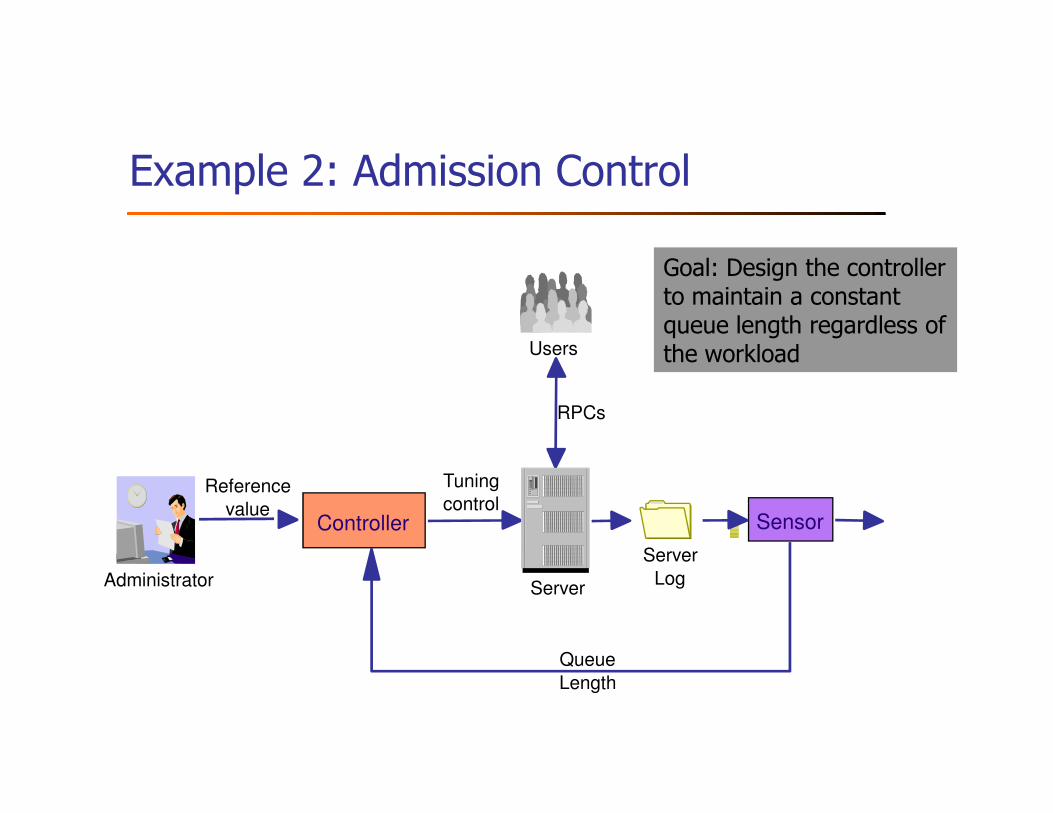
Example 2: Admission Control

Users

RPCs

Goal: Design the controller to maintain a constant queue length regardless of the workload

Administrator

Controller

RPCs

Sensor

Server

Reference

value

Queue

Length

Tuning

control

Server

Log

Open-loop control

� Compute control input without continuous variable measurement

� Simple

� Need to know EVERYTHING ACCURATELY to work right

Cruise-control car: friction(t), ramp_angle(t)� Cruise-control car: friction(t), ramp_angle(t)

� E-commerce server: Workload (request arrival rate? resource consumption?); system (service time? failures?)

� Open-loop control fails when

� We don’t know everything

� We make errors in estimation/modeling

� Things change

Feedback (close-loop) Control

Actuatorcontrol

inputmanipulated

variable

Controlled System

control

function

Controller

Monitor

reference

input

controlled

variable

variable

+-

error

function

sample

� Measure variables and use it to compute control input

� More complicated (so we need control theory)

� Continuously measure & correct

� Cruise-control car: measure speed & change engine force

� E-commerce server: measure response time & admission control

� Embedded network: measure collision & change backoff window

� Feedback control theory makes it possible to control well even if

� We don’t know everything

� We make errors in estimation/modeling

� Things change

Why feedback control?Open, unpredictable environments

� Deeply embedded networks: interaction with physical environments

� Number of working nodes

� Number of interesting events� Number of interesting events

� Number of hops

� Connectivity

� Available bandwidth

� Congested area

� Internet: E-business, on-line stock broker

� Unpredictable off-the-shelf hardware

Why feedback control?We want QoS guarantees

� Deeply embedded networks� Update intruder position every 30 sec

� Report fire <= 1 min

� E-business server� Purchase completion time <= 5 sec

� Throughput >= 1000 transaction/sec

� The problem:

provide QoS guarantees in open, unpredictable environments

Advantages of feedback control theory

� Adaptive resource management heuristics� Laborious design/tuning/testing iterations

� Not enough confidence in face of untested workload

Queuing theory� Queuing theory� Doesn’t handle feedbacks

� Not good at characterizing transient behavior in overload

� Feedback control theory� Systematic approach to analysis and design

� Transient response

� Consider sampling times, control frequency

Taxonomy of basic controls; � Taxonomy of basic controls;

Select controller based on desired characteristics

� Predict system response to some input

� Speed of response (e.g., adjust to workload changes)

� Oscillations (variability)

� Approaches to assessing stability and limit cycles

Example: Control & Response in an Email Server

Control(MaxUsers)

Response(queue length)

GoodBad

13

SlowUseless

Examples of CT in CS

� Network flow controllers (TCP/IP – RED)

� C. Hollot et al. (U.Mass)

� Lotus Notes admission control

� S. Parekh et al. (IBM)

� QoS in Caching

� C. Lu et al. (U.Va)

� Apache QoS differentiation

� C. Lu et al. (U.Va)

Outline

� Examples and Motivation

� Control Theory Vocabulary and Methodology

� Modeling Dynamic Systems

� Transient Behavior Analysis

� Standard Control Actions

� Advanced Topics

� Issues for Computer Systems

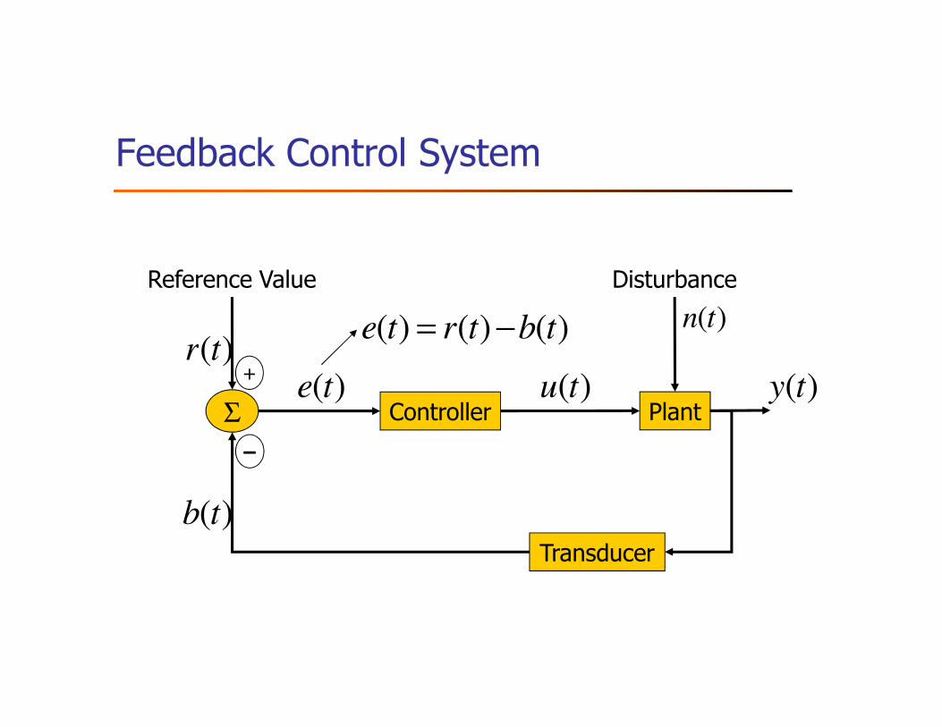
Feedback Control System

)(tn

Disturbance

)(tr)()()( tbtrte −=

+

Reference Value

PlantControllerΣ)(tu )(ty

)(tr)(te

Transducer

)(tb

+

–

Controller Design Methodology

Block diagram

construction

Start

Controller Design

System Modeling

Model Ok?

Stop

Transfer function formulation and

validation

Objective achieved

?

Controller Evaluation

Y

Y

N N

Control System Goals

� Regulation� thermostat, target service levels

� Tracking� robot movement, adjust TCP window to network bandwidthrobot movement, adjust TCP window to network bandwidth

� Optimization� best mix of chemicals, minimize response times

Outline

� Examples and Motivation

� Control Theory Vocabulary and Methodology

� Modeling Dynamic Systems

� Transient Behavior Analysis

� Standard Control Actions

� Advanced Topics

� Issues for Computer Systems

System Models

� Linear vs. non-linear

� Principle of superposition: for linear systems, the net response at a given place and time caused by two or more stimuli is the sum of the responses which would have been caused by each stimulus individually.

� Deterministic vs. Stochastic

� Time-invariant vs. Time-varying� Are coefficients functions of time?

� Continuous-time vs. Discrete-time� t ∈ R vs. k ∈ Z

Approaches to System Modeling

� First Principles� Based on known laws

� Physics, Queueing theory

� Difficult to do for complex systems

� Experimental (System ID)� Experimental (System ID)� Statistical/data-driven models

� Requires data

� Is there a good “training set”?

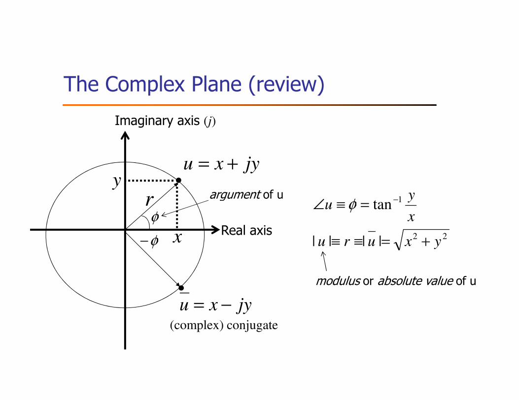
The Complex Plane (review)

Imaginary axis (j)

jyxu +=y

1tany

u =≡∠ −φr argument of u

Real axisxφ

φ−

jyxu −=(complex) conjugate

22

1

||||

tan

yxuru

x

yu

+=≡≡

=≡∠ −φr argument of u

modulus or absolute value of u

Basic Tool For Continuous Time: Laplace Transform

� Convert time-domain functions and operations into frequency-domain

∫∞

−==0

)()()]([ dtetfsFtfst

L

frequency-domain

� f(t) → F(s) (t∈�, s∈�)

� Linear differential equations (LDE) → algebraic expression in Complex plane

� Graphical solution for key LDE characteristics

� Discrete systems use the analogous z-transform

Laplace Transforms of Common Functions

Name f(t) F(s)

Impulse

Step

1

11)( =tf

>

==

00

01)(

t

ttf

Step

Ramp

Exponential

Sine

s

1

2

1

s

as −

1

22

1

s+ω

1)( =tf

ttf =)(

atetf =)(

)sin()( ttf ω=

Properties of Laplace Transform

1)(

)0()()(ationDifferenti

)()()]()([calingAddition/S2121

sF

fssFtfdt

dL

sbFsaFtbftafL

±−=

±=±

[ ] [ ]

[ ]

)(lim)(lim theoremvalueFinal

)(lim)0( theoremvalueInitial

)()()nConvolutio

)(1)(

)(nIntegratio

0

210 21

0

ssFtf-

ssFf-

sFsFdτ(ττ)f(tfL

dttfss

sFdttfL

st

s

t

t

→∞→

∞→

±=

=

=+

=∫ −

∫+=∫

Insights from Laplace Transforms

� What does the Laplace Transform say about f(t)?

� Value of f(0)

� Initial value theorem

Value of f(t) at steady state (if it converges)� Value of f(t) at steady state (if it converges)

� Final-value theorem

� Does f(t) converge to a finite value?

� Poles of F(s): whether within unit circle

� Does f(t) oscillate?

� Poles of F(s) : whether the imaginary part is 0

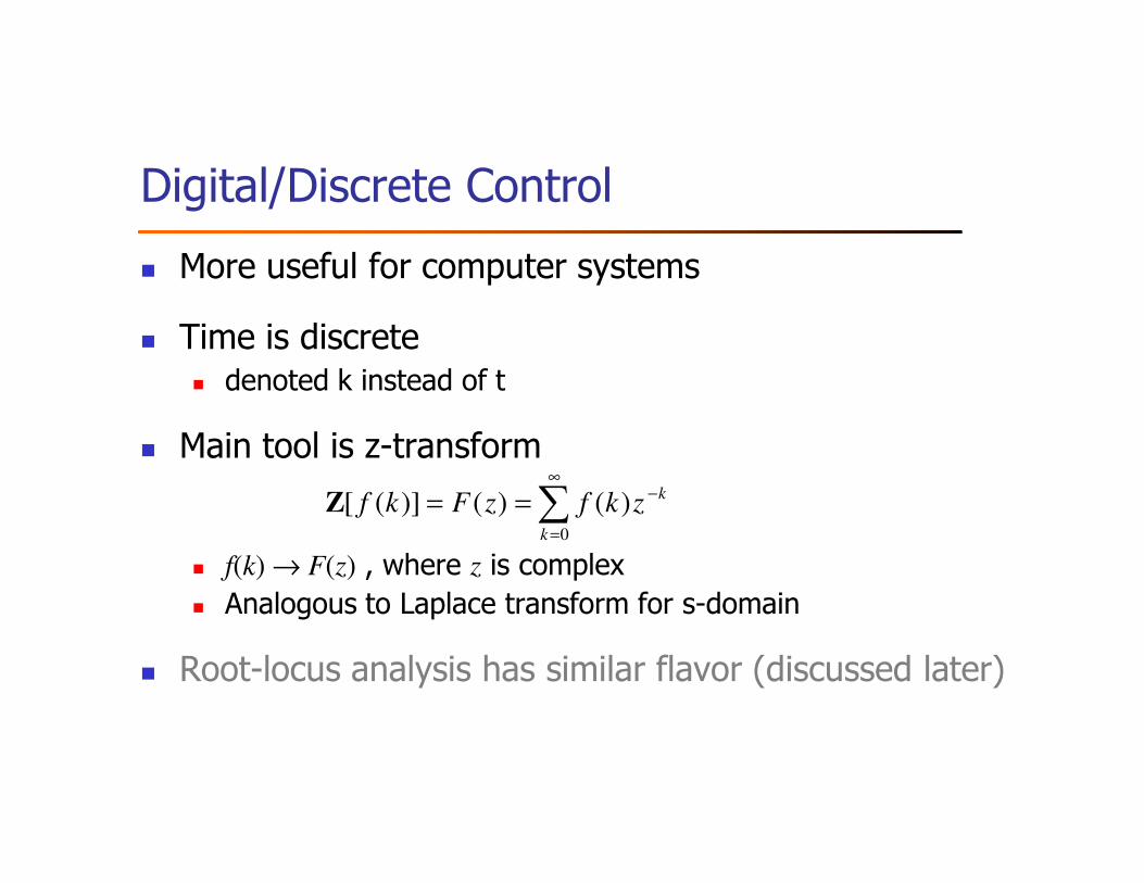
Digital/Discrete Control

� More useful for computer systems

� Time is discrete� denoted k instead of t

� Main tool is z-transform� Main tool is z-transform

� f(k) → F(z) , where z is complex

� Analogous to Laplace transform for s-domain

� Root-locus analysis has similar flavor (discussed later)

∑∞

=

−==0

)()()]([k

kzkfzFkfZ

z-Transforms of Common Functions

Name f(t) F(z)

Impulse

Step

1

z1)( =tf

F(s)

1

1

>

==

00

01)(

t

ttf

Step

Ramp

Exponential

Sine

1−z

z

2)1( −z

z

aez

z

−

1)(Cos2

Sin2 +− zz

z

ω

ω

1)( =tf

ttf =)(

atetf =)(

)sin()( ttf ω=

s

1

2

1

s

as −

1

22

1

s+ω

Properties of z-Transforms

V(z)U(z) Y(z)v(k) u(k)y(k)

aU(z)Y(z)kauky

Addition

)()( Scaling

Transform- Z Domain Time Property

+=+=

==

)zu(n...)u(zU(z)z Y(z)n) u(ky(k)

)zU(z)-zu( Y(z)) u(ky(k)

U(z)zY(z) u(k-n) y(k)

U(z)z Y(z) ) u(k-y(k)

nn

-n

-

10 shift -n

01 shift Unit

delay -n

1 delay Unit 1

−−−−=+=

=+=

==

==

Z-Transform: Final Value Theorem

� Z-Transform provides a convenient way to determine the steady state value

of a signal, if one exists

� Allows us to determine if steady state error exists (among other things):

Theorem: If all of the poles of (1 ) ( ) lie within the unit circle, thenz Y z−

1

Theorem: If all of the poles of (1 ) ( ) lie within the unit circle, then

lim ( ) lim ( 1) ( )k z

z Y z

y k z Y z∞

−

= −uuur uuur

Example

2

1 1

0.11 0.11( )

1.6 0.6 ( 1)( 0.6)

0.11( 1) ( ) | | 0.275

0.6z z

z zY z

z z z z

zz Y z

z= =

− −= =

− + − −

−− = = −

−

0 5 10 15-0.35

-0.3

-0.25

-0.2

-0.15

-0.1

-0.05

0

k

y(k

)

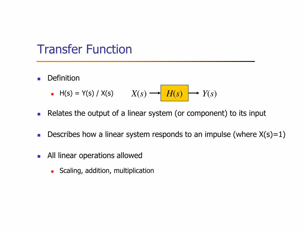
Transfer Function

� Definition

� H(s) = Y(s) / X(s)

� Relates the output of a linear system (or component) to its input

H(s)X(s) Y(s)

Relates the output of a linear system (or component) to its input

� Describes how a linear system responds to an impulse (where X(s)=1)

� All linear operations allowed

� Scaling, addition, multiplication

Block Diagrams

� Pictorially expresses flows and relationships between

elements in system

� Blocks may recursively be systems� Blocks may recursively be systems

� Rules

� Cascaded elements: convolution

� Summation and difference elements

� Can simplify

Block Diagram of System

)(sU

)(sN

Disturbance

)(sR

)(sE+ )(1 sG )(2 sG

Reference Value

PlantControllerΣ)(sU

)(sY

)(sE

Transducer

)(sB

+

–

Σ

)(1 sG )(2 sG

)(sH

Combining Blocks

Σ

)(sR)(sE

+ )())()((21

sGsNsG +

Reference Value

Combined BlockΣ)(sY

)(sE

Transducer

)(sB

–

)(sH

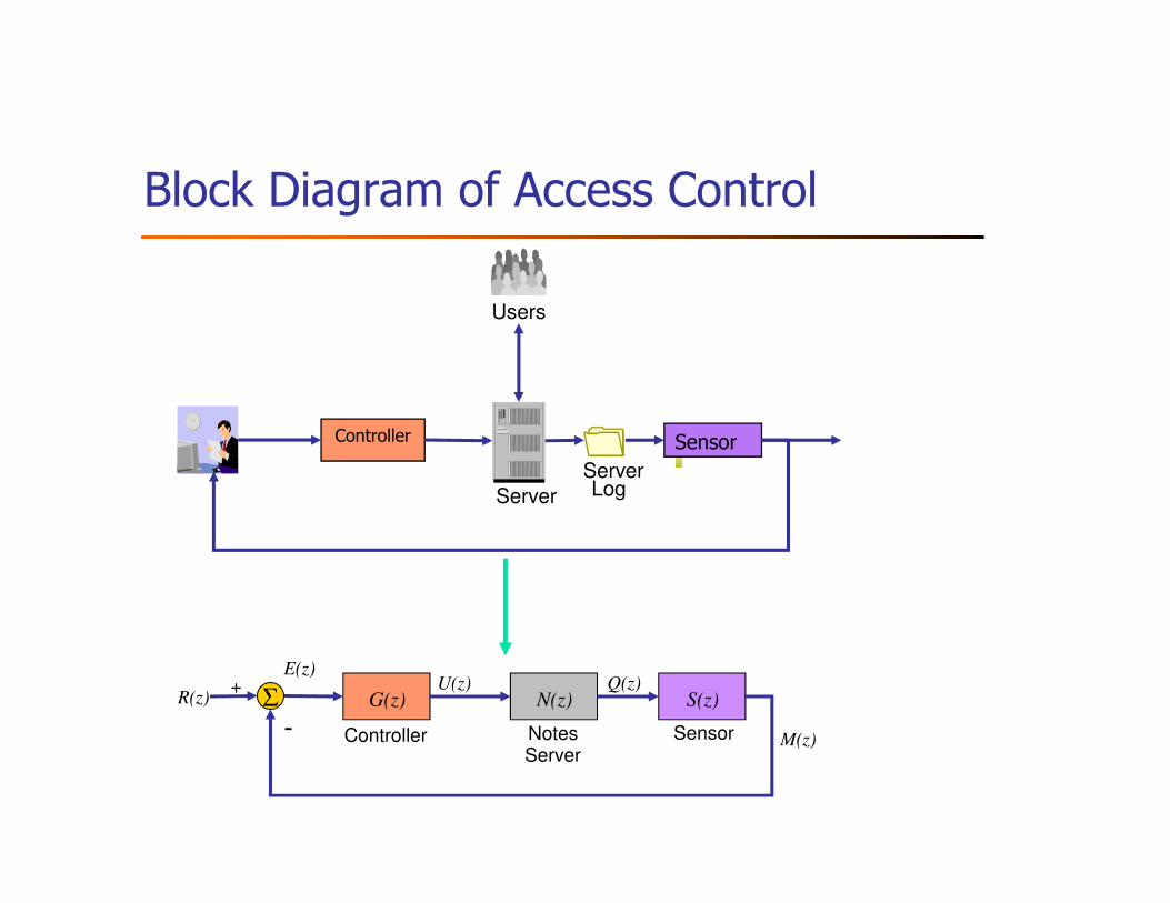
Block Diagram of Access Control

Users

Controller Sensor

M(z)

G(z) N(z) S(z)

Controller Notes Server

Sensor

R(z)+

E(z)U(z)

-

Q(z)Σ

Sensor

Server

ServerLog

Key Transfer Functions

PlantControllerΣ)(sU

)(sY

)(sR)(sE+

–

)(1 sG )(2 sG

Reference

)()()(1

)()(

)(

)( :

21

21

sHsGsG

sGsG

sR

sY

+=Feedback

)()()(

)(

)(

)(

)(

)(21 sGsG

sE

sU

sU

sY

sE

sY== :eedforwardF

)()()()(

)(21 sHsGsG

sE

sB= :Loop-penO

Transducer

)(sB

–

)(sH

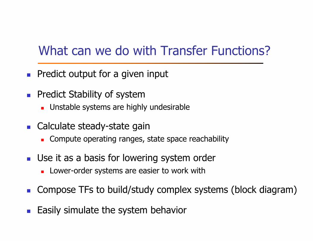
What can we do with Transfer Functions?

� Predict output for a given input

� Predict Stability of system

� Unstable systems are highly undesirable

Calculate steady-state gain� Calculate steady-state gain

� Compute operating ranges, state space reachability

� Use it as a basis for lowering system order

� Lower-order systems are easier to work with

� Compose TFs to build/study complex systems (block diagram)

� Easily simulate the system behavior

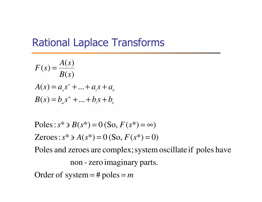
Rational Laplace Transforms

bsbsbsB

asasasA

sB

sAsF

m

m

n

n

...)(

...)(

)(

)()(

01

01

+++=

+++=

=

m

sFsAs

sFsBs

bsbsbsBm

poles # system ofOrder

parts.imaginary zero-non

have poles if oscillate system complex; are zeroes and Poles

)0*)( (So, 0*)(* :Zeroes

)*)( (So, 0*)(* :Poles

...)(01

==

==∋

∞==∋

+++=

Bounded Signals

Discrete Integrator

y(k)u(k)

0 1 2 3 4 50

0.2

0.4

0.6

0.8

1

1.2 Step Input

0 1 2 3 4 50

1

2

3

4

5Ramp Output

1.2 Impulse Input

1.2 Delayed Step Output

yu

k k

Which of these outputs are undesirable?

0

5a=1.2

0

0.5

1

Definition:{u(k)} is bounded if 9 constant M such that |u(k)| · M for all k.

39

0 1 2 3 4 50

0.2

0.4

0.6

0.8

1

1.2

0 1 2 3 4 50

0.2

0.4

0.6

0.8

1

1.2

yu

k k

-5

0 5 10-5

0

5a=-1.2

0 10 20 30 40 50 60 70-1

-0.5

0

0.5

10 2 4 6 8

-1

-0.5

0 5 10 15 200

0.2

0.4

0.6

0.8

1

Lets Formalize this…

BIBO Stability

� NOTE: Bad reaction to unbounded inputs is OK?!

� Are these systems BIBO stable?

Definition:A system is BIBO stable if for any bounded input {u(k)}, its output {y(k)} is bounded.

� Are these systems BIBO stable?

Unity y(k+1) = 1

P Controller y(k+1) = KP u(k)

Integrator y(k+1) = y(k) + u(k)

I Controller y(k+1) = y(k) + KI u(k)

M/M/1/K y(k+1) = 0.49y(k) + 0.033u(k)

Mystery y(k+1) = -1.3y(k) + 2.3u(k)

There must be a better way…

BIBO Stability Theorem

Theorem:

A system G(z) is BIBO stable iff all the poles of G(z) are inside the unit circle.

System Time domain Eq Transfer Function Poles

Unity y(k+1) = 1 G(z) = 1 N/AUnity y(k+1) = 1 G(z) = 1 N/A

P Controller y(k+1) = KP u(k) G(z) = KP N/A

Integrator y(k+1) = y(k) + u(k) G(z) = 1/(z-1) z=1

I Controller y(k+1) = y(k) + KI u(k) G(z) = KI/(z-1) z=1

M/M/1/K y(k+1) = 0.49y(k) + 0.033u(k) G(z) = 0.033/(z-0.49) z = 0.49

Mystery y(k+1) = -1.3y(k) + 2.3u(k) G(z) = 2.3/(z+1.3) z = -1.3

Steady-state Gain

� G(z) can be used to characterize steady-state reaction of system

� Reaction to a constant input

� Given

� BIBO stable system G(z)

� Apply step input U(z)� Apply step input U(z)

NOTE

� Output MUST converge

� Definition: Steady-state Gain (aka DC Gain)

ss

ssSSGainu

y=

� Theorem: Steady state gain of a system G(z) is given by G(1)

� Proof

� System response to a unit step (ie uss=1) is given by

Steady-state Gain Theorem

1)()(

−=

z

zzGzY

� Applying final-value theorem to get yss

� For a general ARX transfer function, steady-state gain is

)1(

)(lim

1)()1(lim

)()1(lim)(lim

1

1

1ss

G

zzG

z

zzGz

zYzkyy

z

z

zk

=

=

−−=

−==

→

→

→∞→

n

m

aa

bbG

−−−

++=

L

L

1

1

1)1(

)1(...)(

)1(...)()1(

1

1

+−++

++−++=+

mkubkub

nkyakyaky

m

n

System Order

� System order = # poles

� Same as n in ARX formula

� Same as # initial conditions needed to seed the difference

equationequation

� Why does it matter?

� “Complexity” of system response proportional to system order

� Higher (¸ 2nd) order systems have complex poles

� Implies oscillatory factors in system response

� More difficult to design/analyze higher-order systems

Simulating Transfer Functions

� For complex transfer functions, cannot analyze

� Solution: Simulate

)(1

1

1

1

azaz

zbzbzG

n

nn

mn

m

n

−−−

++=

−

−−

L

L

� Inputs

� Initial conditions (depends on system order)

� u(k)

)(...)1(

)(...)1()(

1

1

1

mkubkub

nkyakyaky

azaz

m

n

n

−++−+

−++−=

−−−

:to equivalent is

L

Transfer Functions: Summary

� Transfer Functions are also expressed as polynomials in z

� We can predict BIBO stability from the poles of a TF

� We can calculate steady-state gain from a TF

We can build simplified TF from a high-order TF that has similar � We can build simplified TF from a high-order TF that has similar steady-state gain and settling time (see Chapter 6 of [1])

� It is usually easy to convert a difference eq to a TF

� Can usually plug into the general ARX form

� One can simulate a TF by converting back to difference equation

First Order System

sT

K

sTK

K

sR

sY

+≈

++=

11)(

)(

Reference

)(sY

)(sR

Σ)(sE

1)(sB

)(sUsT+1

1K

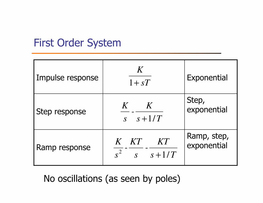
First Order System

Impulse response Exponential

Step,

1 sT

K

+

KKStep response

Step, exponential

Ramp response

Ramp, step, exponential

/1

2Ts

KT-

s

KT-

s

K

+

/1

Ts

K-

s

K

+

No oscillations (as seen by poles)

Second Order System

)04 (ie,part imaginary zero-non have poles if Oscillates

2)(

)( :response Impulse

2

22

2

2

JKB

ssKBsJs

K

sR

sY

NN

N

<−

++=

++=

ωξω

ω

:frequency natural Undamped

2 where :ratio Damping

)04 (ie,part imaginary zero-non have poles if Oscillates

J

K

JKBB

B

JKB

N

c

c

=

==

<−

ω

ζ

Second Order System: Parameters

0)Im0,(Re overdamped :1

Im) 0(Re dunderdampe :10

0)Im 0,(Ren oscillatio undamped :0

:ratio damping oftion Interpreta

ζ

ζ

ζ

=≠≤

≠≠<<

≠==

systems) mechanicalfor vibrationfree offrequency (or

n oscillatio theoffrequency thegives

:frequency natural undamped oftion Interpreta

0)Im0,(Re overdamped :1

Nω

ζ =≠≤

Outline

� Examples and Motivation

� Control Theory Vocabulary and Methodology

� Modeling Dynamic Systems

� Transient Behavior Analysis

� Standard Control Actions

� Advanced Topics

� Issues for Computer Systems

� References

Objectives of Control for Computing Systems: SASO

� Stability

� Accuracy

� Settling time

� Overshoot

Characteristics of Transient Response

Overshoot

Controlled

variable

±ε±ε±ε±ε%Steady state error

Reference

Settling timeTime

Steady StateTransient State

Reference

Rise time

Transient Response

� Estimates the shape of the curve based on the

foregoing points on the x and y axis

� Typically applied to the following inputs� Typically applied to the following inputs

� Impulse

� Step

� Ramp

� Quadratic (Parabola)

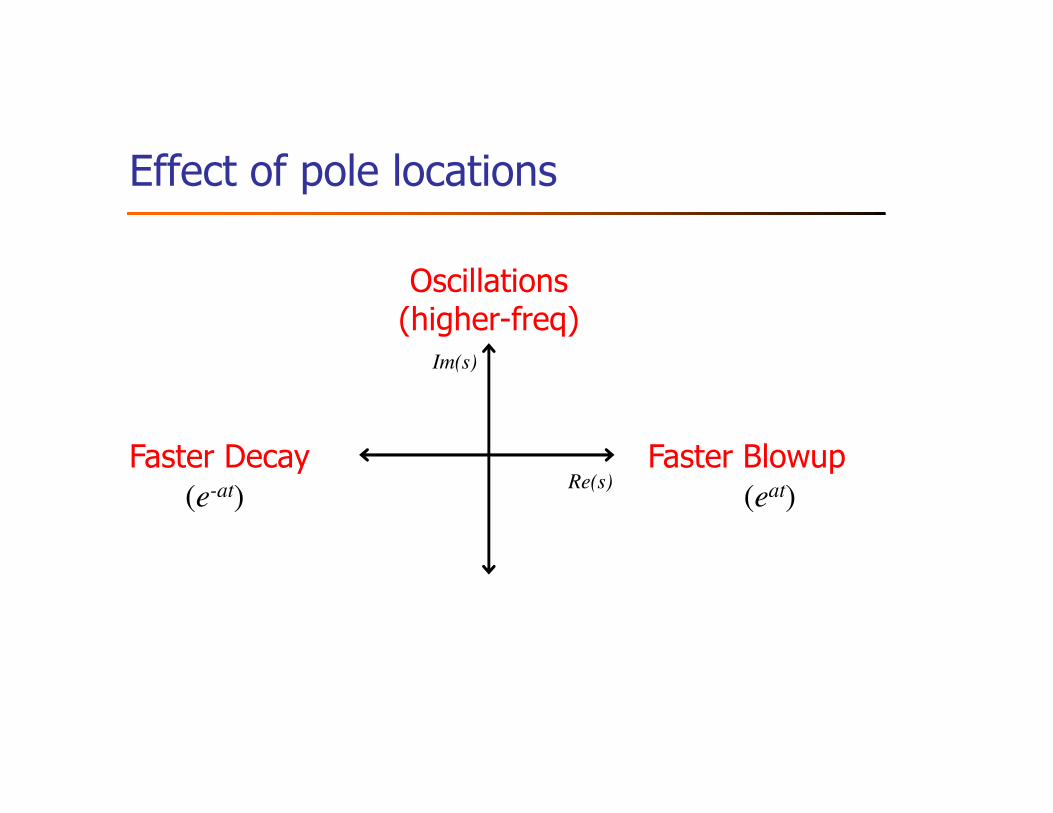
Effect of pole locations

Oscillations(higher-freq)

Im(s)

Faster Decay Faster BlowupRe(s)

(e-at) (eat)

Root-locus Analysis

� Based on characteristic eqn of closed-loop transfer function

� Plot location of roots of this eqn� Same as poles of closed-loop transfer function

Parameter (gain) varied from 0 to ∞� Parameter (gain) varied from 0 to ∞

� Multiple parameters are ok� Vary one-by-one

� Plot a root “contour” (usually for 2-3 params)

� Quickly get approximate results� Range of parameters that gives desired response

Root Locus analysis of Discrete Systems

� Stability boundary: |z|=1 (Unit circle)

� Settling time: distance from Origin

Oscillation frequency/speed: location relative to Im. axis� Oscillation frequency/speed: location relative to Im. axis

� Right half => slower

� Left half => faster

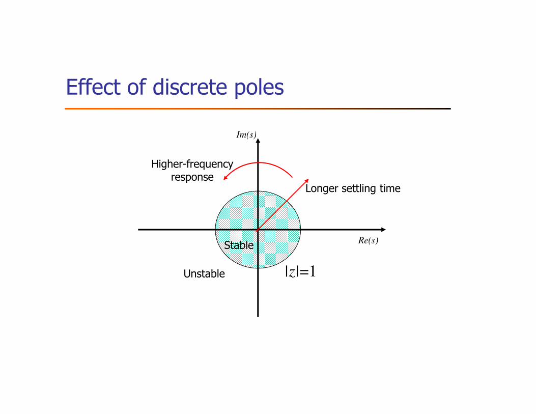
Effect of discrete poles

Longer settling time

Im(s)

Higher-frequencyresponse

|z|=1

Re(s)

Unstable

Stable

System ID for Admission Control

M(z)

G(z) N(z) S(z)

Controller Notes Server

Sensor

R(z)+

E(z)U(z)

-

Q(z)Σ

Transfer FunctionsARMA Models

Control Law

Transfer Functions

δzz

zK

cz

dzd

az

zbzGzSzN i 1

1)()()(

1

10

1

0

−−

+

−=Open-Loop:

δzz

zKzG

cz

dzdzS

az

zbzN

i 1

1)(

)(

)(

1

10

1

0

−=

−

+=

−=

)()1()(

)1()()1()(

)()1()(

101

01

teKtutu

tqdtqdtmctm

tubtqatq

i+−=

−++−=

+−=

Root Locus Analysis of Admission Control

Predictions:•Ki small => No controller-induced oscillations•Ki large => Some oscillations•Ki v. large => unstable system (delay=2)•Usable range of Ki for delay=2 is small

Experimental Results

Control(MaxUsers)

Response(queue length)

GoodBad

SlowUseless

Outline

� Examples and Motivation

� Control Theory Vocabulary and Methodology

� Modeling Dynamic Systems

� Transient Behavior Analysis

� Standard Control Actions

� Advanced Topics

� Issues for Computer Systems

� References

Basic Control Actions: u(t)

:control Integral

:control alProportion

KsUdtteKtu

KsE

sUteKtu

i

t

pp

==

==

∫)(

)()(

)(

)()()(

:control alDifferenti

:control Integral

sKsE

sUte

dt

dKtu

s

K

sE

sUdtteKtu

dd

i

i

==

== ∫

)(

)()()(

)(

)()()(

0

Effect of Control Actions

� Proportional Action� Adjustable gain (amplifier)

� May have non-zero steady-state error

� Integral ActionEliminates bias (steady-state error)� Eliminates bias (steady-state error)

� Can cause oscillations

� Derivative Action (“rate control”)

� Effective in transient periods

� Provides faster response (higher sensitivity)

� Never used alone

Basic Controllers

� Proportional control is often used by itself

� Integral and differential control are typically used in

combination with at least proportional controlcombination with at least proportional control

� eg, Proportional Integral (PI) controller:

+=+==

sTK

s

KK

sE

sUsG

i

p

I

p

11

)(

)()(

Summary of Basic Control

� Proportional control� Multiply e(t) by a constant

� PI control� Multiply e(t) and its integral by separate constants

Avoids bias for step� Avoids bias for step

� PD control� Multiply e(t) and its derivative by separate constants

� Adjust more rapidly to changes

� PID control� Multiply e(t), its derivative and its integral by separate

constants

� Reduce bias and react quickly

Outline

� Examples and Motivation

� Control Theory Vocabulary and Methodology

� Modeling Dynamic Systems

� Transient Behavior Analysis

� Standard Control Actions

� Advanced Topics

� Issues for Computer Systems

� References

Advanced Control Topics

� Robust Control

� Can the system tolerate noise?

� Adaptive Control

� Controller changes over time (adapts)

MIMO Control� MIMO Control

� Multiple inputs and/or outputs

� Stochastic Control

� Controller minimizes variance

� Optimal Control

� Controller minimizes a cost function (e.g., function of error)

� Nonlinear systems

� Challenging to derive analytic results

Outline

� Examples and Motivation

� Control Theory Vocabulary and Methodology

� Modeling Dynamic Systems

� Transient Behavior Analysis

� Standard Control Actions

� Advanced Topics

� Issues for Computer Systems

Issues for Computer Science

� Most systems are non-linear� But linear approximations may do

� E.g., fluid approximations

� First-principles modeling is difficultUse empirical techniques� Use empirical techniques

� Control objectives are different� Optimization rather than regulation

� Multiple Controls� State-space techniques

� Advanced non-linear techniques (eg, NNs)

References

� Control Theory Basics

� [1] Joseph L. Hellerstein, Yixin Diao, Sujay Parekh, Dawn M. Tilbury, Feedback Control of Computing Systems, Wiley-IEEE Press, 2004. (ISBN: 978-0-471-26637-2)

� [2] G. Franklin, J. Powell and A. Emami-Naeini. “Feedback Control of Dynamic Systems, 3rd

ed”. Addison-Wesley, 1994.

� [3] K. Ogata. “Modern Control Engineering, 3rd ed”. Prentice-Hall, 1997.

� [4] K. Ogata. “Discrete-Time Control Systems, 2nd ed”. Prentice-Hall, 1995.

� Applications in Computer Science

� C. Hollot et al. “Control-Theoretic Analysis of RED”. IEEE Infocom 2001

� C. Lu, et al. “A Feedback Control Approach for Guaranteeing Relative Delays in Web Servers”. IEEE Real-Time Technology and Applications Symposium, June 2001.

� S. Parekh et al. “Using Control Theory to Achieve Service-level Objectives in Performance Management”. Int’l Symposium on Integrated Network Management, May 2001

� Y. Lu et al. “Differentiated Caching Services: A Control-Theoretic Approach”. Int’l Conf on Distributed Computing Systems, Apr 2001

� S. Mascolo. “Classical Control Theory for Congestion Avoidance in High-speed Internet”. Proc. 38th Conference on Decision & Control, Dec 1999

� S. Keshav. “A Control-Theoretic Approach to Flow Control”. Proc. ACM SIGCOMM, Sep 1991

� D. Chiu and R. Jain. “Analysis of the Increase and Decrease Algorithms for Congestion Avoidance in Computer Networks”. Computer Networks and ISDN Systems, 17(1), Jun 1989