An introduction to diffractive tomographic microscopy O. Haeberlé1, A. Sentenac2 and H. Giovannini2 1Laboratoire MIPS/Groupe LabEl, Université de Haute-Alsace, IUT de Mulhouse, 61 rue Albert Camus,
68093 Mulhouse cédex - France 2Institut Fresnel - UMR 6133 CNRS, Bâtiment Fresnel, Campus de St Jérome, 13397 Marseille cédex 20 -
France We present the principles of diffractive tomographic microscopy. Contrary to classical transmission mi-croscopy, this technique is based on a coherent, monochromatic, polarized illumination of the specimen, and records the diffracted light in both amplitude and phase using a holographic detection set-up. Com-bined with multiple illuminations of the specimen, a tomography is performed, and a numerical recon-struction of the index of refraction distribution within the specimen is obtained.
The optical microscope has become an invaluable tool for biology thanks to its unique capabilities to image living specimens in three dimensions, and over long periods (time-lapse microscopy), due to the non-ionizing nature of light. The fluorescence techniques are particularly appreciated because they allow a specific labelling of cellular structures. However, fluorescent markers may induce unfavourable effects like photo-toxicity and they do not allow an overall imaging of the sample. As a consequence, among the many techniques, which have been developed, those permitting to observe a specimen without the need for specific staining have known a regain of interest in the recent years. One quotes, for example, the Second-Harmonic Generation microscopy (SHG), the Coherent Anti-Stokes Raman Spectroscopy microscopy (CARS) and the conventional transmission microscopy. In transmis-sion microscopy (classical, phase-contrast or Differential Interference Contrast), the image is formed by a complex interaction of the incoherent illuminating light with the specimen. The recorded contrast, while very helpful for morphological studies, does not yield quantitative information on the opto-geometrical characteristics of the sample. In particular, the optical index of refraction distribution within the specimen is difficult to reconstruct. On the contrary, the use of coherent light illumination, combined with an interferometric detection, permits one to record holograms, which encode both the amplitude and phase of the light diffracted by the specimen. Using an adapted model of diffraction (typically the first order Born approximation), this so-called holographic microscopy allows for the reconstruction of the specimen index of refraction dis-tribution. When this technique is combined with either a rotation of the specimen or an inclination of the illumination wave, the set of recorded holograms represents a diffractive tomographic acquisition, which permits 3-D reconstructions of much better quality.
2. Basics of diffraction and its application to imaging
The aim of this short paragraph is to recall the relation-ship between the opto-geometrical characteris-tics of an object and its diffracted field. This link is at the core of most imaging systems that use waves for probing samples. For simplicity, we will assume the scalar approximation. Accounting for the vecto-rial nature of electromagnetic waves does not change the main lines of the presentation. The interested reader can complete this rapid introduction by the lecture of any textbook on electromagnetism or wave diffraction, for example [1].
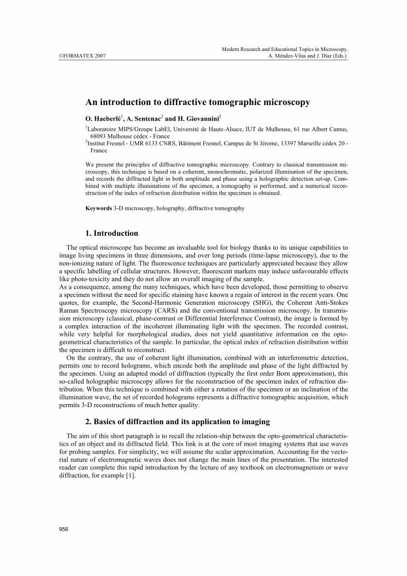
Fig. 1 A plane wave depicted by its wavevector kinc illu-minates an object characterized by its relative contrast of permittivity ∆ε. The diffracted field is decomposed into a sum of plane waves of wavevectors k.
We consider (Figure 1) an object in vacuum defined by its relative permittivity ε(r) and illuminated by a monochromatic incident wave, with wavelength λ = 2πc/ω stemming from a source S(r). Hereafter, the exp(-iωt) dependence is omitted. The total scalar field obeys the Helmholtz equation:
)()()()()( 20
20 rrrrr SEkEkE +ε∆=+∆ , (1)
where k0 is the wavenumber 2π/λ, and the contrast of permittivity ∆ε = 1-ε. Ιntroducing the Green func-tion of Eq. (1):
G(r) = -exp(ik0r)/4πr , (2)
we obtain the integral equation for the total field,
where Einc is the field generated by S that would exist in absence of the object. The support of the integral in (3) is limited to the geometrical support Ω of the object. When the observation point r is far from the object, r’2/λ<<r, with r’ in Ω, the diffracted field can be written as:
)(4
)exp()( 0 kr eπr
rikEd −= , rk ˆ0k= , (4)
where
r'r'r'k.r'k dEike )()()exp()( 20 ε∆−= ∫ . (5)
We now suppose that the incident field is a plane wave with wavevector kinc, Einc(r) = Ainc exp(ikinc.r), and that the object is weakly diffracting so that the field inside Ω is close to Einc (Born approximation [2]). In this case, Eq. (5) yields:
)(~),( incinc Ce kkkk −ε∆= , (6)
where C = Ainck02. Equation (6) provides a one to one correspondence between the diffracted far-field
amplitude and the Fourier coefficient of the relative permittivity of the object. It is at the basis of most far-field imaging technique such as X-ray diffraction tomography [3], acoustic tomography [4] and, as will be seen later in section 5, digital holographic microscopy [5]. Note that an expression similar to Eq. (6) is obtained in the vectorial case by replacing C by a vector whose direction is given by the pro-jection of the incident field polarization Ainc onto the plane normal to the wavevector k [1].
3. Conventional microscopy
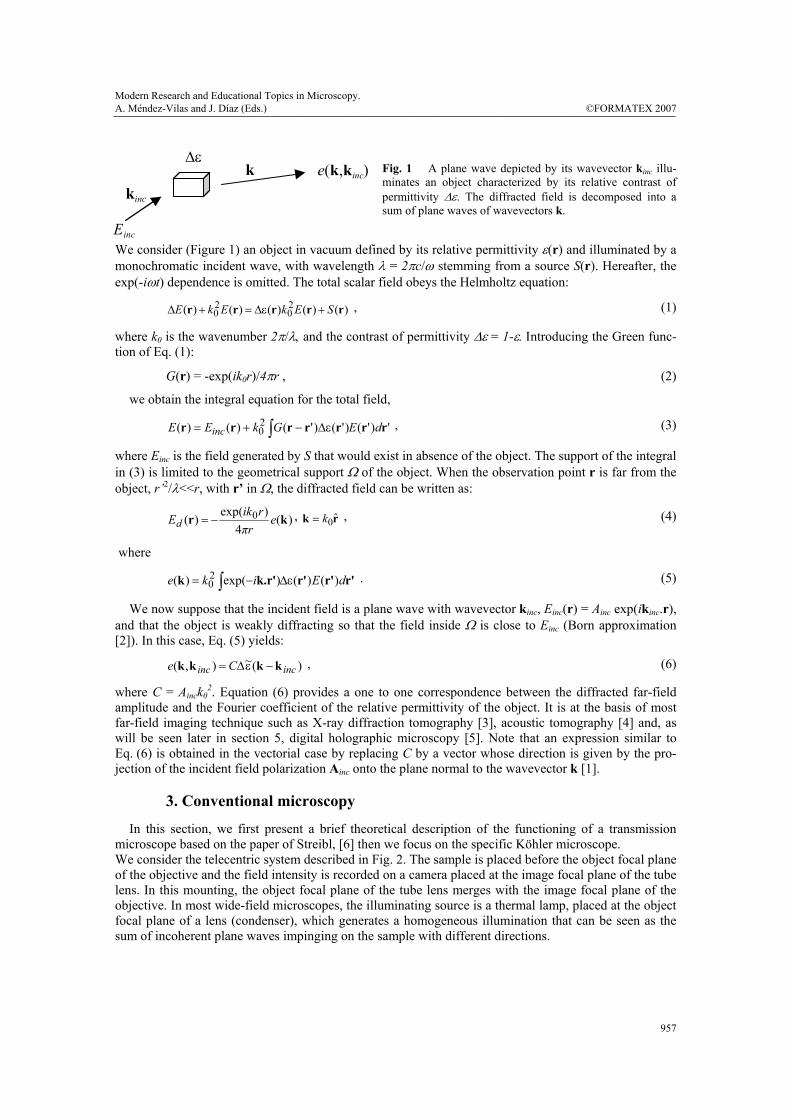
In this section, we first present a brief theoretical description of the functioning of a transmission microscope based on the paper of Streibl, [6] then we focus on the specific Köhler microscope. We consider the telecentric system described in Fig. 2. The sample is placed before the object focal plane of the objective and the field intensity is recorded on a camera placed at the image focal plane of the tube lens. In this mounting, the object focal plane of the tube lens merges with the image focal plane of the objective. In most wide-field microscopes, the illuminating source is a thermal lamp, placed at the object focal plane of a lens (condenser), which generates a homogeneous illumination that can be seen as the sum of incoherent plane waves impinging on the sample with different directions.
Fig. 2 Principle of detection of the diffracted wave in a classical transmission microscope
Due to the incoherence properties, the detected intensity on the camera can be considered as the sum of the intensities obtained for each incident plane wave. Hence, we will first consider the case where the object is illuminated by a unique plane wave with wavevector kinc and amplitude Ainc. The formation of the image in a microscope relies entirely on the analogical Fourier transform that is performed by the lenses. Indeed, under certain conditions, one can show that the field existing at the image plane of the lens is proportional to the Fourier transform of the field existing at the object focal plane. Hence, in the set-up presented in Fig. 2, one verifies that the field existing in the image plane of the tube lens, namely the CCD plane, will be equal to that existing at the object focal plane of the objec-tive, i. e. very close to the sample. Yet, the field recovery is incomplete due to the loss of information stemming from propagation and the finite collection cone of the objective. Actually, the imaging system acts as low-pass filter, symbolized by the pupil placed in the image plane of the objective that cuts all the transverse Fourier components of the field that are above k0sinθ where θ is the collection angle of the objective, as shown in Fig. 2, and defines the numerical aperture of the microscope through sinθ =NA (for the sake of simplicity, we consider a microscope in air). More precisely, under the paraxial approxi-mation, the field at the object plane of the objective, EO, can be written as a Fourier integral:
where e(k) is the far-field diffracted amplitude defined in the previous section with k|| the projection of k on the (x,y) plane. In the image plane of the microscope, the field EI can be cast in the form:
where p(u) indicates the filtering function of the imaging set-up. p(u) is a radial function equal to zero if u > k0NA and one elsewhere. From Eq. (8), it is seen that, by measuring the complex field EI in the im-age plane of a microscope and performing a Fourier transform, one retrieves the far-field amplitude e(k) within the limited solid angle defined by the numerical aperture of the objective. This property will be used in Sections 4 and 5 to build a numerical holographic microscope. In a conventional microscope however, one detects the field intensity |EI|2, i. e. the interference between the incident and the diffracted field1. In this case, the relation-ship between the measured data and the permittivity of the objects is much more complex than the one-to-one correspondence pointed out in Eq. (6). With an incoherent illumination set-up the detected intensity is the sum of |EI|2 for all possible kinc. Long but relatively simple calculations using Eq. (8), Eq. (6) and assuming that the amplitude of the diffracted field is much smaller than that of the incident field, show that the detected intensity is propor-tional to the permittivity contrast ∆ε of the object, convolved with a point spread function that is different for the real and the imaginary part of ∆ε. This particularity forbids any efficient deconvolution operation for restoring the image. For absorptive objects and equal illumination and collection solid angle, the point spread function P(r||) in the (x,y) plane is given by:
P(r||) = | J1(k0NAr||/k0NA r||) |2 . (9) 1 In dark-field microscopes, the angle of the incident waves is bigger than the collection angle of the objective, i. e. kinc||>k0sinθ. In
this case, the field that exists at the image plane of the microscope is only the diffracted field.
From this formula, one retrieves the classical Abbe criterion that states that two point objects will be distinguished on the image only if their interdistance is larger than 0.5λ/NA. The very general analysis provided in this section can be adapted to most microscopes set-up. Among those commonly used in biology, one may mention:
- Brightfield microscopy: it is well suited for specimens naturally presenting an important contrast in amplitude. If necessary, dyes may be used to improve the contrast. - Darkfield microscopy: specimens with a low contrast are difficult to image in brigthfield mi-croscopy. Darkfield microscopy is an alternative, in which the specimen is illuminated with light normally not collected by the microscope objective. Only light scattered by the specimen is de-tected, and the latter appears brighter than the black background. Rheinberg illumination is a vari-ant, using coloured filters. Oblique illumination is another possible approach. - Polarized microscopy detects variations of optical pathways, related to the thickness and index of refraction of the specimen. A coloured contrast is produced. - Phase contrast microscopy makes use of the phase difference the diffracted rays experience, when compared to non-diffracted ones. These rays interfere to form an image with higher contrast (a variant is Hoffman illumination). - Differential interference contrast (DIC) microscopy combines feature of polarized microscopy and phase contrast microscopy in order to increase the contrast.
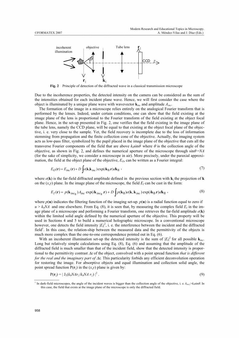
In the following, we stick to brightfield microscopy, and parallel it with diffractive optical tomogra-phy. Figure 3 recalls Fig. 1, but describes in more details the principle of Köhler illumination. The illu-mination source is incoherent, and both spatially and angularly extended. The condenser collects the emitted radiation and concentrates it onto the specimen. The light diffracted by the specimen is collected by the objective, and refocused so as to form the image onto the detector (here the retina). The benefit of Köhler illumination is to ensure a uniform illumination of the sample by defocusing as much as possible the image of the source. At the same time, the image of the specimen onto the detector is properly formed. Hence, the illumination source, which is not distinguishable from the light reemitted by the specimen, forms a uniform background on the detector. It degrades the recorded image essentially by reducing its contrast. Note that, in fluorescence microscopy, the fluorescence wavelength is slightly shifted with respect to the illumination wavelength (Stokes shift). As a result, a filter permits to collect only the light emitted by the sample.
Specimen Objective Eye-piece
Source
Object conjugate planes Aperture conjugate planes
Eye-piecediaphragm
Fielddiaphragm
Objective backfocal plane
Condenseraperture
Source
Condenser
Fig. 3 Principle of Köhler illumination. The role of the condenser is to illuminate the specimen under the largest possible range of angles. The role of the objective is to collect waves, which are diffracted by the specimen, under the largest possible angles.
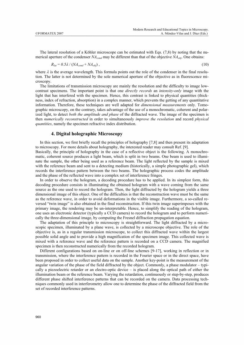
The lateral resolution of a Köhler microscope can be estimated with Eqs. (7,8) by noting that the nu-merical aperture of the condenser NAcond may be different than that of the objective NAobj. One obtains:
Rlat = 0.5λ / (NAcond + NAobj) , (10)
where λ is the average wavelength. This formula points out the role of the condenser in the final resolu-tion. The latter is not determined by the sole numerical aperture of the objective as in fluorescence mi-croscopy. The limitations of transmission microscopy are mainly the resolution and the difficulty to image low-contrast specimens. The important point is that one directly records an intensity-only image with the light that has interfered with the specimen. Hence, this contrast is linked to physical quantities (thick-ness, index of refraction, absorption) in a complex manner, which prevents the getting of any quantitative information. Therefore, these techniques are well adapted for dimensional measurements only. Tomo-graphic microscopy, on the contrary, takes advantage of the use of a monochromatic, coherent and polar-ized light, to detect both the amplitude and phase of the diffracted wave. The image of the specimen is then numerically reconstructed in order to simultaneously improve the resolution and record physical quantities, namely the specimen refractive index distribution.
4. Digital holographic Microscopy
In this section, we first briefly recall the principles of holography [7,8] and then present its adaptation to microscopy. For more details about holography, the interested reader may consult Ref. [9]. Basically, the principle of holography in the case of a reflective object is the following. A monochro-matic, coherent source produces a light beam, which is split in two beams. One beam is used to illumi-nate the sample, the other being used as a reference beam. The light reflected by the sample is mixed with the reference beam and sent to a detecting medium (historically, a simple photographic gel), which records the interference pattern between the two beams. The holographic process codes the amplitude and the phase of the reflected wave into a complex set of interference fringes. In order to observe the hologram, a decoding procedure has to be applied. In its simplest form, this decoding procedure consists in illuminating the obtained hologram with a wave coming from the same source as the one used to record the hologram. Then, the light diffracted by the hologram yields a three dimensional image of this object. One of the difficulties is that the reconstruction wave must be the same as the reference wave, in order to avoid deformations in the visible image. Furthermore, a so-called re-versed “twin image” is also obtained in the final reconstruction. If this twin image superimposes with the primary image, the rendering may be un-interpretable. Hence, to simplify the reading of the hologram, one uses an electronic detector (typically a CCD camera) to record the hologram and to perform numeri-cally the three-dimensional image, by computing the Fresnel diffraction propagation equation. The adaptation of this principle to microscopy is straightforward. The light diffracted by a micro-scopic specimen, illuminated by a plane wave, is collected by a microscope objective. The role of the objective is, as in a regular transmission microscope, to collect this diffracted wave within the largest possible solid angle and to provide a high magnification of the specimen image. This collected wave is mixed with a reference wave and the reference pattern is recorded on a CCD camera. The magnified specimen is then reconstructed numerically from the recorded hologram. Different configurations based on on-line or on off-line schemes [9-17], working in reflection or in transmission, where the interference pattern is recorded in the Fourier space or in the direct space, have been proposed in order to collect useful data on the sample. Another key-point is the measurement of the angular variation of the phase of the field diffracted by the object. Commonly, a phase modulator – typi-cally a piezoelectric retarder or an electro-optic device – is placed along the optical path of either the illumination beam or the reference beam. Varying the retardation, continuously or step-by-step, produces different phase shifted interference patterns that can be recorded on the camera. Data processing tech-niques commonly used in interferometry allow one to determine the phase of the diffracted field from the set of recorded interference patterns.
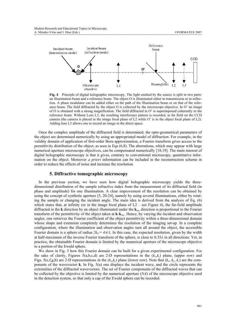
Fig. 4 Principle of digital holographic microscopy. The light emitted by the source is split in two parts: an illumination beam and a reference beam. The object O is illuminated either in transmission or in reflec-tion. A phase modulator can be added either on the path of the illumination beam or on that of the refer-ence beam. The field diffracted by the object O is collected by the microscope objective. In O’ an image of O is obtained with a strong magnification. The field diffracted in O’ is superimposed coherently to the reference beam. Without Lens L3, the resulting interference pattern is recorded, in far field on the CCD camera (the camera is placed in the image focal plane of L2 while O’ is in the object focal plane of L2). Adding lens L3 allows one to record an image in the direct space.
Once the complex amplitude of the diffracted field is determined, the opto-geometrical parameters of the object are determined numerically by using an appropriated model of diffraction. For example, in the validity domain of application of first-order Born approximation, a Fourier transform gives access to the permittivity distribution of the object, as seen in Eqs (6,8). The aberrations, which may appear with large numerical aperture microscope objectives, can be compensated numerically [18,19]. The main interest of digital holographic microscopy is that it gives, contrary to conventional microscopy, quantitative infor-mation on the object. Moreover a priori information can be included in the reconstruction scheme in order to reduce the effects of noise and increase the resolution.
5. Diffractive tomographic microscopy
In the previous section, we have seen how digital holographic microscopy yields the three-dimensional distribution of the sample refractive index from the measurement of its diffracted field (in phase and amplitude) for one illumination. A clear improvement of the resolution can be obtained by using the concept of synthetic aperture [5, 20-24], namely by using several illuminations, either by rotat-ing the sample or changing the incident angle. The main idea is derived from the analysis of Eq. (6) which states that, at infinity (or in the image focal plane of L2 – see Figure 4), the far-field amplitude diffracted in the k direction by an object illuminated under the kinc direction is proportional to the Fourier transform of the permittivity of the object taken at k-kinc. Hence, by varying the incident and observation angles, one retrieves the Fourier coefficient of the object permittivity within a three-dimensional domain whose shape and extension completely determines the resolution of the imaging set-up. In a complete configuration, where the illumination and observation angles turn all around the object, the accessible Fourier domain is a sphere of radius 2k0 = 4π/λ. In this case, the expected resolution, given by the width at half-maximum of the inverse Fourier transform of the sphere, is close to 0.35λ in all directions. Yet, in practice, the obtainable Fourier domain is limited by the numerical aperture of the microscope objective to a portion of the Ewald sphere. We show in Fig. 5 how this Fourier domain can be built for a given experimental configuration. For the sake of clarity, Figures 5(a,b,c,d) are 2-D representations in the (kx,kz) plane, (upper row) and Figs. 5(e,f,g,h) are 2-D representations in the (kx,ky) plane (lower row). Note that (kx, ky, kz) are the com-ponents of the wavevector k. In Fig. 5(a) one displays the incident wave, and the circle represents the extremities of the diffracted wavevectors. The set of Fourier components of the diffracted waves that can be collected by the objective is limited by the numerical aperture (NA) of the microscope objective used in the detection system, so that only a cap of the Ewald sphere can be recorded.
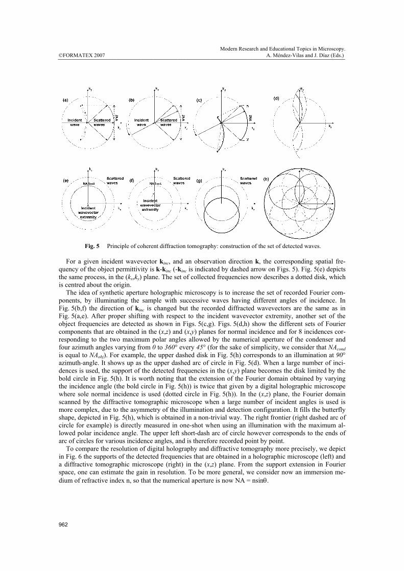
Fig. 5 Principle of coherent diffraction tomography: construction of the set of detected waves. For a given incident wavevector kinc, and an observation direction k, the corresponding spatial fre-quency of the object permittivity is k-kinc (-kinc is indicated by dashed arrow on Figs. 5). Fig. 5(e) depicts the same process, in the (kx,ky) plane. The set of collected frequencies now describes a dotted disk, which is centred about the origin. The idea of synthetic aperture holographic microscopy is to increase the set of recorded Fourier com-ponents, by illuminating the sample with successive waves having different angles of incidence. In Fig. 5(b,f) the direction of kinc is changed but the recorded diffracted wavevectors are the same as in Fig. 5(a,e). After proper shifting with respect to the incident wavevector extremity, another set of the object frequencies are detected as shown in Figs. 5(c,g). Figs. 5(d,h) show the different sets of Fourier components that are obtained in the (x,z) and (x,y) planes for normal incidence and for 8 incidences cor-responding to the two maximum polar angles allowed by the numerical aperture of the condenser and four azimuth angles varying from 0 to 360° every 45° (for the sake of simplicity, we consider that NAcond is equal to NAobj). For example, the upper dashed disk in Fig. 5(h) corresponds to an illumination at 90° azimuth angle. It shows up as the upper dashed arc of circle in Fig. 5(d). When a large number of inci-dences is used, the support of the detected frequencies in the (x,y) plane becomes the disk limited by the bold circle in Fig. 5(h). It is worth noting that the extension of the Fourier domain obtained by varying the incidence angle (the bold circle in Fig. 5(h)) is twice that given by a digital holographic microscope where sole normal incidence is used (dotted circle in Fig. 5(h)). In the (x,z) plane, the Fourier domain scanned by the diffractive tomographic microscope when a large number of incident angles is used is more complex, due to the asymmetry of the illumination and detection configuration. It fills the butterfly shape, depicted in Fig. 5(h), which is obtained in a non-trivial way. The right frontier (right dashed arc of circle for example) is directly measured in one-shot when using an illumination with the maximum al-lowed polar incidence angle. The upper left short-dash arc of circle however corresponds to the ends of arc of circles for various incidence angles, and is therefore recorded point by point. To compare the resolution of digital holography and diffractive tomography more precisely, we depict in Fig. 6 the supports of the detected frequencies that are obtained in a holographic microscope (left) and a diffractive tomographic microscope (right) in the (x,z) plane. From the support extension in Fourier space, one can estimate the gain in resolution. To be more general, we consider now an immersion me-dium of refractive index n, so that the numerical aperture is now NA = nsinθ.
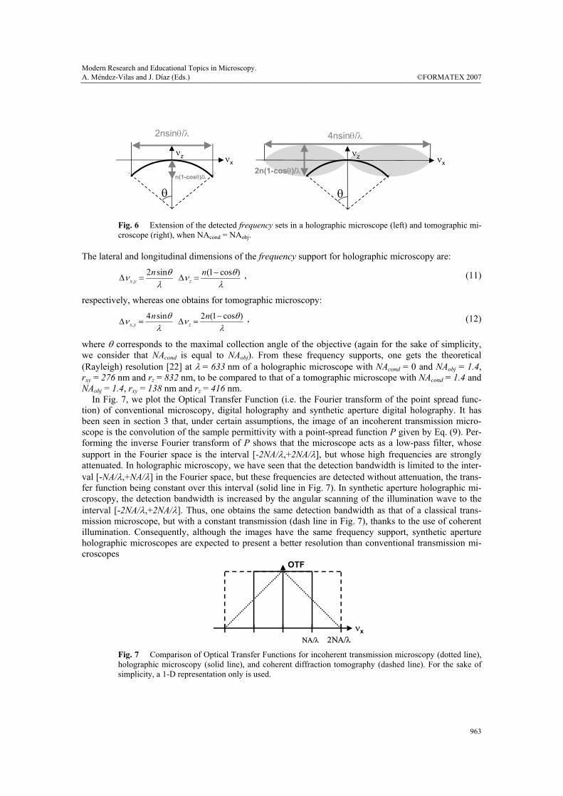
Fig. 6 Extension of the detected frequency sets in a holographic microscope (left) and tomographic mi-croscope (right), when NAcond = NAobj.
The lateral and longitudinal dimensions of the frequency support for holographic microscopy are:
∆ν x,y =2n sinθ
λ ∆ν z =
n(1− cosθ)λ
, (11)
respectively, whereas one obtains for tomographic microscopy:
∆ν x,y =4n sinθ
λ ∆ν z =
2n(1− cosθ)λ
, (12)
where θ corresponds to the maximal collection angle of the objective (again for the sake of simplicity, we consider that NAcond is equal to NAobj). From these frequency supports, one gets the theoretical (Rayleigh) resolution [22] at λ = 633 nm of a holographic microscope with NAcond = 0 and NAobj = 1.4, rxy = 276 nm and rz = 832 nm, to be compared to that of a tomographic microscope with NAcond = 1.4 and NAobj = 1.4, rxy = 138 nm and rz = 416 nm. In Fig. 7, we plot the Optical Transfer Function (i.e. the Fourier transform of the point spread func-tion) of conventional microscopy, digital holography and synthetic aperture digital holography. It has been seen in section 3 that, under certain assumptions, the image of an incoherent transmission micro-scope is the convolution of the sample permittivity with a point-spread function P given by Eq. (9). Per-forming the inverse Fourier transform of P shows that the microscope acts as a low-pass filter, whose support in the Fourier space is the interval [-2NA/λ,+2NA/λ], but whose high frequencies are strongly attenuated. In holographic microscopy, we have seen that the detection bandwidth is limited to the inter-val [-NA/λ,+NA/λ] in the Fourier space, but these frequencies are detected without attenuation, the trans-fer function being constant over this interval (solid line in Fig. 7). In synthetic aperture holographic mi-croscopy, the detection bandwidth is increased by the angular scanning of the illumination wave to the interval [-2NA/λ,+2NA/λ]. Thus, one obtains the same detection bandwidth as that of a classical trans-mission microscope, but with a constant transmission (dash line in Fig. 7), thanks to the use of coherent illumination. Consequently, although the images have the same frequency support, synthetic aperture holographic microscopes are expected to present a better resolution than conventional transmission mi-croscopes
νx
OTF
ΝΑ/λ 2ΝΑ/λ Fig. 7 Comparison of Optical Transfer Functions for incoherent transmission microscopy (dotted line), holographic microscopy (solid line), and coherent diffraction tomography (dashed line). For the sake of simplicity, a 1-D representation only is used.
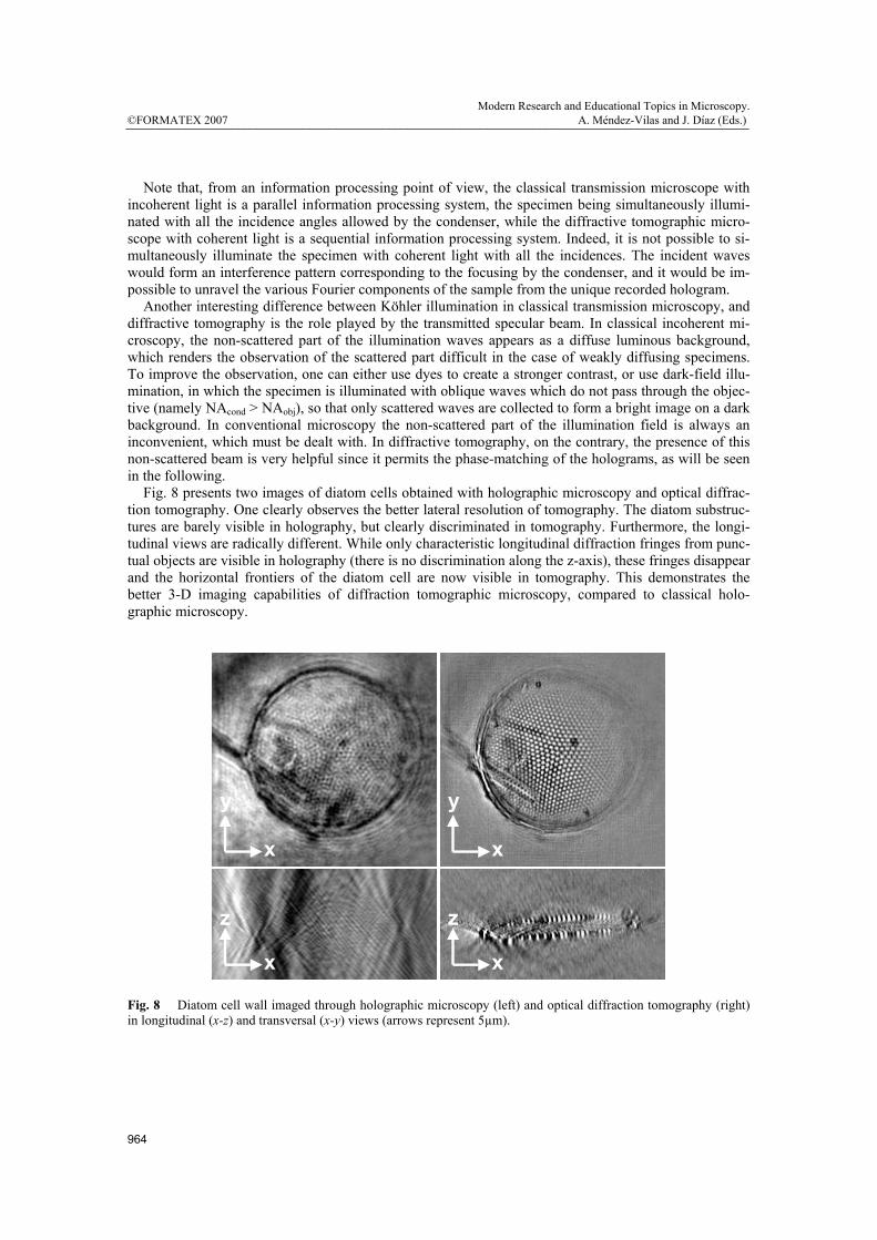
Note that, from an information processing point of view, the classical transmission microscope with incoherent light is a parallel information processing system, the specimen being simultaneously illumi-nated with all the incidence angles allowed by the condenser, while the diffractive tomographic micro-scope with coherent light is a sequential information processing system. Indeed, it is not possible to si-multaneously illuminate the specimen with coherent light with all the incidences. The incident waves would form an interference pattern corresponding to the focusing by the condenser, and it would be im-possible to unravel the various Fourier components of the sample from the unique recorded hologram. Another interesting difference between Köhler illumination in classical transmission microscopy, and diffractive tomography is the role played by the transmitted specular beam. In classical incoherent mi-croscopy, the non-scattered part of the illumination waves appears as a diffuse luminous background, which renders the observation of the scattered part difficult in the case of weakly diffusing specimens. To improve the observation, one can either use dyes to create a stronger contrast, or use dark-field illu-mination, in which the specimen is illuminated with oblique waves which do not pass through the objec-tive (namely NAcond > NAobj), so that only scattered waves are collected to form a bright image on a dark background. In conventional microscopy the non-scattered part of the illumination field is always an inconvenient, which must be dealt with. In diffractive tomography, on the contrary, the presence of this non-scattered beam is very helpful since it permits the phase-matching of the holograms, as will be seen in the following. Fig. 8 presents two images of diatom cells obtained with holographic microscopy and optical diffrac-tion tomography. One clearly observes the better lateral resolution of tomography. The diatom substruc-tures are barely visible in holography, but clearly discriminated in tomography. Furthermore, the longi-tudinal views are radically different. While only characteristic longitudinal diffraction fringes from punc-tual objects are visible in holography (there is no discrimination along the z-axis), these fringes disappear and the horizontal frontiers of the diatom cell are now visible in tomography. This demonstrates the better 3-D imaging capabilities of diffraction tomographic microscopy, compared to classical holo-graphic microscopy.
x
z
x
z
x
y
x
y
Fig. 8 Diatom cell wall imaged through holographic microscopy (left) and optical diffraction tomography (right) in longitudinal (x-z) and transversal (x-y) views (arrows represent 5µm).
Hence, it has been shown that the resolution of diffractive tomographic microscopy is, in principle, better than that of a conventional microscope. Yet, this achievement is obtained at a certain expense. We now describe the main problems raised by this relatively new technique. The first issue is to illuminate and observe the sample along various directions. One solution consists in rotating the sample while keeping the illumination and detection static [25]. This set-up has the advan-tage that the optical interferometer has no moving parts, which is favourable in terms of vibrations or alignments. However, keeping a precise rotation at the microscopic scale, compatible with interferomet-ric measurements can be very difficult. Furthermore, this set-up necessitates placing the observed sample in a rotating microcapillary. This procedure has proven to work well for individual cells or pollen grains, for example, but is not favoured by biologists, who often prefer to handle biological samples between a glass slide and a coverglass. Furthermore, using a rotating capillary oblige to use a longer working dis-tance objective with a lower numerical aperture, at the detriment of the resolution. It is therefore prefer-able to keep the specimen static. For technical reasons, it is then easier to rotate the illumination than to rotate the detection, which would need to rotate both the reference beam and the collected diffracted beam, which have to interfere [22]. The second issue is the retrieval, for numerous successive illuminations, of the amplitude and phase of the diffracted field from an interference pattern. We assume that the optical path difference between the illumination and the reference beams is constant during the acquisition of each hologram corresponding to one incidence. However, between two illuminations, the phase between the illumination and the refer-ence beams may change due to thermal/mechanical drifts or simply because the optical paths of the illu-mination beam are different for the various incidence angles. This variation leads to a phase shift be-tween the holograms. For retrieving the complex Fourier components of the sample from the synthetic hologram, one has to compensate for these phase shifts by phase-matching the holograms. This can be done by considering the shared spatial frequencies detected at two different incidence angles. Common spatial frequencies correspond to the condition : k-kinc=k’-k’inc, where kinc and k’inc are the two incident wavevectors, k and k’ are two diffracted wavevector. Within the validity of Born approximation, Eq. (6), the phases of the diffracted amplitude e(k,kinc) and e(k’,k’inc) are to be equal. If this is not the case, a phase matching of the two holograms is performed by adding a constant phase to one of the holograms. This procedure, adopted for all the recorded holograms, compensates for the random phase drifts. Other techniques based on the measurement of the phase between the reference beam and the non-scattered light (i.e. the specular transmitted beam), have also been proposed [22]. A frequency analysis and a nu-merical post-processing of the data [26] can also be used. Note that the detection of the diffracted field can be performed in different ways, either in the Fourier plane [22,24], (in the image focal plane of L2 in Fig. 4) or in the image plane [23] (by adding the lens L3 in Fig. 4). The main drawback of the measurements in the Fourier space comes from the fact that the specular beam (the non-scattered light) is focused onto a small surface of the camera and may saturate the detector. Attenuating too strongly the incident beam is not possible because it would lead to a low signal-to-noise ratio in the regions of low intensity on the camera. For solving this problem, one can use a variable density on the illumination beam. For each incidence angle, two holograms can be recorded and processed: one at low incident intensity, which serves to measure the incident beam, together with the low frequency part of the spectrum, another at strong intensity, which serves to measure the high frequency components [22]. Data fusion techniques then permit to reconstruct the spectrum without saturation near the frequency origin. Measurements in the image plane avoid this drawback. In this case, for each incidence, a Fourier transform is performed to retrieve the hologram in the Fourier space as in the previous case. The calculated holograms are then processed in order to obtain the synthetic hologram. Another important point of this technique is the calibration of the diffracted intensity. The latter is necessary if one wants to obtain quantitative information on the sample [26]. For this purpose, the field diffracted by a sample with known opto-geometrical parameters has to be measured. A comparison with the results predicted by theory allows one to calibrate the system by normalizing the value of the dif-fracted intensities.
From section 2, we have seen that, under the Born approximation, the permittivity distribution of the object can be recovered, from the measured complex amplitude of the diffracted field, thanks to a Fourier transform. Depending on the opto-geometrical parameters of the object, other models of diffraction can be used. For example, the profile of a reflecting surface can be obtained by using Fraunhofer approxima-tion. In this case, the complex amplitude of the diffracted field is given by,
IIIIIIIIII krkkrkk diRe incinc ]).-(exp[)(),( ∫∫= , (13)
where R(r||)=R0exp[2k0h(r||)] is the reflectivity of the object with R0 being the reflection coefficient of the surface and h(r||) the local height of the object. Hence, calculating the Fourier transform of the diffracted field gives access to h(r||). Approximate models of diffraction allow one to retrieve, with simple inversion schemes, the opto-geometrical parameters of the object from its diffracted far-field. Most of them are based on the single scattering approximation, which is valid essentially for weakly scattering samples. Yet, in certain cases they do not describe properly the diffraction phenomenon. Typically, when the objects are greater than the illuminating wavelength and for strong permittivity contrasts, one needs to account for multiple scat-tering. In this case, iterative reconstruction algorithms based on a rigorous theory of diffraction, which basically, requires to solve Eq. (3), have to be used [27-29]. These algorithms are widely used for im-agery applications in the radiofrequency domain where single scattering assumption does not often hold. Note that, when multiple scattering occurs, the diffracted far-field may gives access to information corre-sponding to spatial frequencies of the field that do not propagate (namely the evanescent components). Indeed, multiple scattering produces a coupling between the spatial frequencies and e(k,kinc) is no more a function of k-kinc. For this reason, a resolution better than the Rayleigh-Abbe limit can be obtained [27-29]. Another way to improve the resolution is to increase the value of the spatial frequency of the incident field in order to extend the available Fourier support of the sample. This can be done, for example, by immerging the sample and the objective into a medium of high refractive index, or by illuminating the sample in total internal reflection, with Total Internal Reflection Tomography, (TIRT) [27-29]. This configuration permits theoretically an improvement of the resolution by a factor of n, where n is the refractive index of the prism used to illuminate the sample. However, since the evanescent field that illuminates the object decreases exponentially as one moves away from the substrate, its application is restricted to surface imaging. Recently [29], it has been proposed to deposit the object onto a sub-lambda grating in order to increase the spatial frequency of the incident field beyond the value given by the available indices of refraction. Indeed, the field above the grating presents arbitrary large spatial frequen-cies. It has been shown theoretically that the resolution of a grating-assisted microscope can be much better than that of TIRT and well beyond the Abbe limit. Another application concerns the statistical characteristics of random objects such as rough surfaces or heterogeneous films. In these cases, the measurement of the phase of the diffracted field gives access to information that cannot be obtained from intensity measurements. In the case of rough surfaces, for ex-ample, it yields the height distribution probability density, which is a more precise characterization of the surface than the power spectral density function classically obtained with intensity measurements.
7. Conclusion
Tomographic microscopy using coherent illumination is a promising technique, because it is expected to have a much better resolution than conventional microscopes with equal numerical aperture. Moreover it gives access to the distribution of the index of refraction within a specimen, a quantity, which is not or very hardly accessible to present microscopes. Yet, using coherent illumination presents some chal-lenges. In particular, one must use a sequential acquisition of the data, and a post-acquisition numerical reconstruction of the image, which limits the speed of acquisition. Moreover, an absolute calibration of
the system is necessary to obtain quantitative information on the index of refraction and still remains to be done. In this review, we have considered only transmission set-ups, but this technique can also be adapted to reflection microscopy. Detecting both the transmitted and the reflected field would pave the way to a high-resolution isotropic 3-D imaging tool for non-labelled transparent specimens. The progress in this domain are continuous, thanks to several research groups, and one can expect to see, in the future, dif-fractive tomographic microscopy (and its simplified version: holographic microscopy) become a routine tool for biology, in complement to other, more-established techniques.
Acknowledgements The authors gratefully acknowledge Patrick Chaumet and Kamal Belkebir for fruitful discus-sions, and Matthieu Debailleuil, Vincent Georges, Vincent Lauer and Bertrand Simon for their enlightening contri-butions and for providing the diatome images to illustrate this article. They also thank Vincent Lauer for interesting discussions about the tomographic technique he developed.
References
[1] JD Jackson, Classical Electrodynamics, Wiley, New York (1999) [2] M. Born and E. Wolf, Principles of Optics, Cambridge University Press, Cambridge (1999) [3] X-ray and Neutron Reflectivitiy Principles and applications, Jean Daillant and Alain Gibaud (Eds), Lecture
Notes in Physics, Springer, Berlin (1999) [4] R. K. Mueller, M. Kaveh and G. Wade, Reconstructive tomography and applications to ultrasonics, Proc IEEE
67, 567 (1979) [5] E. Wolf, Opt. Comm. 1, 153 (1969) [6] N. Streibl, J. Opt. Soc. Am 2, 121 (1985) [7] D. Gabor, Proc. R. Soc. London, Ser. A 197, 454 (1949) [8] D. Gabor, Nature 161, 777-778 (1948) [9] W. Jueptner, U. Schnars, Digital Holography Digital Hologram Recording, Numerical Reconstruction, and
Related Techniques, Springer, Berlin (2005) [10] E Cuche, F Bevilacqua and C Depeursinge, Opt. Lett. 24, 291 (1999) [11] P. Marquet et al., Opt. Lett. 30, 468 (2005) [12] B. Rappaz et al., Opt. Exp. 13, 9361 (2005) [13] C.J. Mann et al., Opt. Exp. 13, 8693 (2005) [14] G. Ingebetouw, A. El Maghnouji, and R. Foster, J. Opt. Soc. Am. A 22, 892 (2005) [15] G. Ingebetouw, J. Opt. Soc. Am. A 23, 2657 (2006) [16] G. Popescu et al., Opt. Lett. 31, 775 (2006) [17] J. Garcia-Sucerquia et al., Appl. Opt. 45, 836 (2006) [18] F. Montfort et al., J. Opt. Soc. Am. A 23, 2944 (2006) [19] T. Colomb et al., J. Opt. Soc. Am. A 23, 3177 (2006) [20] T. Noda, S. Kawata and S. Minami, Appl. Opt. 31, 670 (1992) [21] A.J. Devaney and A. Schatzberg, SPIE Proc. 1767, 62 (1992) [22] V. Lauer, J. Microscopy 205, 165 (2002) [23] V. Mico et al., J. Opt. Soc. Am. A 23, 3162 (2006) [24] SA Alexandrov et al., Phys. Rev. Lett. 97, 168102 (2006) [25] F. Charrière et al., Opt. Lett. 31, 178 (2006) [26] C. Eyraud et al., Appl. Phys. Lett. 89, 244104 (2006) [27] A. Sentenac, P. Chaumet and K. Belkebir, Phys. Rev. Lett. 24, 243901 (2006) [28] P. Chaumet, K. Belkebir and A. Sentenac Opt. Lett. 29, 2740 (2004) [29] K. Belkebir, P. Chaumet and A. Sentenac, J. Opt. Soc. Am. A 23, 586 (2006)