University of Central Florida University of Central Florida

STARS STARS

Electronic Theses and Dissertations, 2004-2019

2005

An Introduction To Hellmann-feynman Theory An Introduction To Hellmann-feynman Theory

David Wallace University of Central Florida

Part of the Mathematics Commons

Find similar works at: https://stars.library.ucf.edu/etd

University of Central Florida Libraries http://library.ucf.edu

This Masters Thesis (Open Access) is brought to you for free and open access by STARS. It has been accepted for

inclusion in Electronic Theses and Dissertations, 2004-2019 by an authorized administrator of STARS. For more

information, please contact STARS@ucf.edu.

STARS Citation STARS Citation Wallace, David, "An Introduction To Hellmann-feynman Theory" (2005). Electronic Theses and Dissertations, 2004-2019. 413. https://stars.library.ucf.edu/etd/413

AN INTRODUCTION TOHELLMANN-FEYNMAN THEORY

by

DAVID B. WALLACEB. A. Florida Gulf Coast University, 2004M. A. T. University of Louisville, 1992

B. A. Carleton College, 1966

A thesis submitted in partial fulfillment of the requirementsfor the degree of Master of Sciencein the Department of Mathematicsin the College of Arts and Sciencesat the University of Central Florida

Orlando, Florida

Spring Term2005

ABSTRACT

The Hellmann-Feynman theorem is presented together with certain allied theorems. The

origin of the Hellmann-Feynman theorem in quantum physical chemistry is described. The

theorem is stated with proof and with discussion of applicability and reliability. Some

adaptations of the theorem to the study of the variation of zeros of special functions and

orthogonal polynomials are surveyed. Possible extensions are discussed.

ii

TABLE OF CONTENTS

1 Introduction . . . . . . . . . . . . . . . . . . . . . . . . . . . . . . . . . . . . . . . . . . . . . . . . . . . . . . . . . . . . . . . . . . . . . . . 1

2 Statement and Proof . . . . . . . . . . . . . . . . . . . . . . . . . . . . . . . . . . . . . . . . . . . . . . . . . . . . . . . . . . . . . . 5

3 The Quantum Chemistry Context . . . . . . . . . . . . . . . . . . . . . . . . . . . . . . . . . . . . . . . . . . . . . . . . . 8

3.1 Electrostatic Theorem . . . . . . . . . . . . . . . . . . . . . . . . . . . . . . . . . . . . . . . . . . . . . . . . . . . . . . . 8

3.2 Integral Hellmann-Feynman Theorem . . . . . . . . . . . . . . . . . . . . . . . . . . . . . . . . . . . . . . 10

3.3 Adiabatic, Virial, and Hypervirial Theorems . . . . . . . . . . . . . . . . . . . . . . . . . . . . . . . .11

4 The Variation of Zeros of Orthogonal Polynomials . . . . . . . . . . . . . . . . . . . . . . . . . . . . . . . . 13

4.1 Sturm-Liouville Operators . . . . . . . . . . . . . . . . . . . . . . . . . . . . . . . . . . . . . . . . . . . . . . . . . .13

4.2 A Second Derivative Version . . . . . . . . . . . . . . . . . . . . . . . . . . . . . . . . . . . . . . . . . . . . . . . 15

4.3 Tridiagonal Matrices . . . . . . . . . . . . . . . . . . . . . . . . . . . . . . . . . . . . . . . . . . . . . . . . . . . . . . . 16

5 The Generalized Eigenvalue Problem . . . . . . . . . . . . . . . . . . . . . . . . . . . . . . . . . . . . . . . . . . . . . 19

6 Conclusion . . . . . . . . . . . . . . . . . . . . . . . . . . . . . . . . . . . . . . . . . . . . . . . . . . . . . . . . . . . . . . . . . . . . . . . 23

Appendix - About Notation . . . . . . . . . . . . . . . . . . . . . . . . . . . . . . . . . . . . . . . . . . . . . . . . . . . . . . . . 25

List of References . . . . . . . . . . . . . . . . . . . . . . . . . . . . . . . . . . . . . . . . . . . . . . . . . . . . . . . . . . . . . . . . . . 27

i

Chapter 1

Introduction

Briefly stated, the Hellmann-Feynman theorem assures that a non-degenerate eigenvalue

of a hermitian operator in a parameter dependent eigensystem varies with respect to the

parameter according to the formula

∂Eν∂ν

=

⟨ψν ,

∂Hν

∂νψν

⟩, (1.1)

provided that the associated normalized eigenfunction, ψν , is continuous with respect to the

parameter, ν.

Neither Feynman nor Hellmann was first to prove it. Beyond that, the origin of the

Hellmann-Feynman theorem is a somewhat clouded history. The formula (1.1) and allied

formulas seem to have first appeared around 1930 with the advent of quantum mechanics.

Researchers involved in the new and exciting field were innovative1. Some innovations came

into widespread use without attribution of origin. A protege of Wolfgang Pauli named Paul

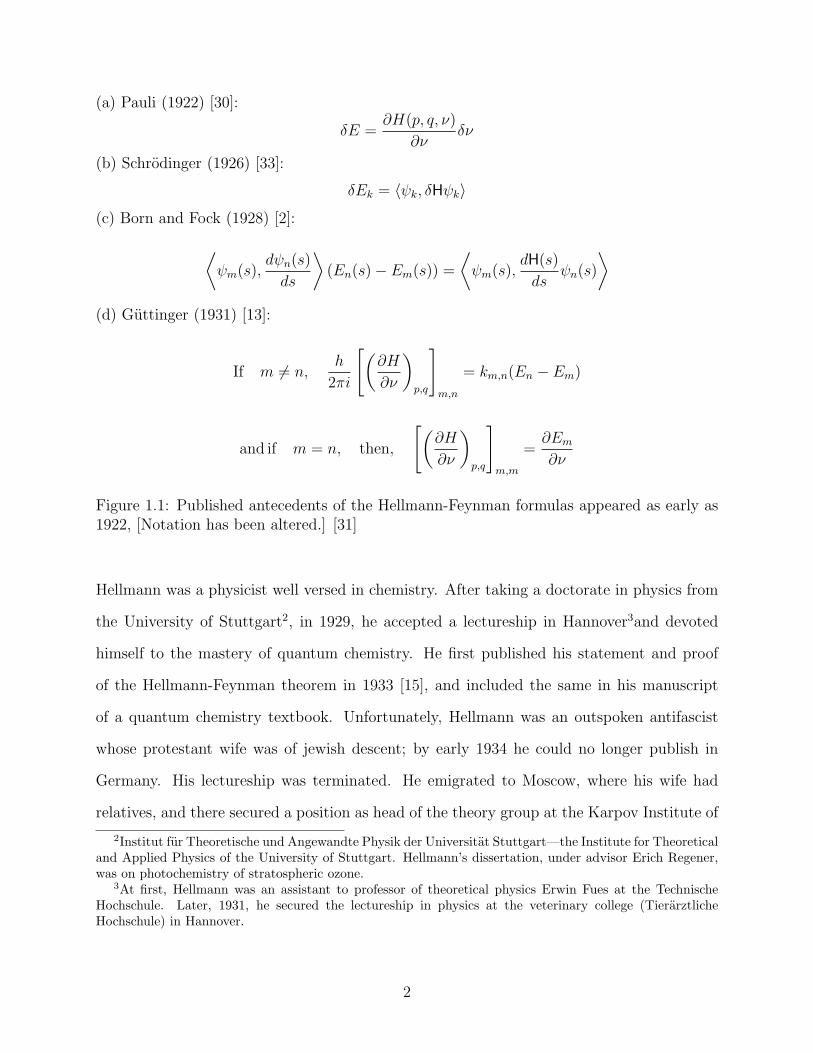
Guttinger may have been the first to publish [13] a careful derivation of the Hellmann-

Feynman formulas, but precursors had appeared at least as early as 1922, see figure 1.

Richard P. Feynman is widely-known, but Hellmann is relatively unknown. Hans G. A.

1When Heisenberg published his 1926 paper on quantum mechanics, he did so without prior knowledgeof the mathematics of matrices. It was only later recognized that the operations Heisenberg described werethe same as matrix multiplication.

1

(a) Pauli (1922) [30]:

δE =∂H(p, q, ν)

∂νδν

(b) Schrodinger (1926) [33]:

δEk = 〈ψk, δHψk〉

(c) Born and Fock (1928) [2]:

⟨ψm(s),

dψn(s)

ds

⟩(En(s)− Em(s)) =

⟨ψm(s),

dH(s)

dsψn(s)

⟩(d) Guttinger (1931) [13]:

If m 6= n,h

2πi

[(∂H

∂ν

)p,q

]m,n

= km,n(En − Em)

and if m = n, then,

[(∂H

∂ν

)p,q

]m,m

=∂Em∂ν

Figure 1.1: Published antecedents of the Hellmann-Feynman formulas appeared as early as1922, [Notation has been altered.] [31]

Hellmann was a physicist well versed in chemistry. After taking a doctorate in physics from

the University of Stuttgart2, in 1929, he accepted a lectureship in Hannover3and devoted

himself to the mastery of quantum chemistry. He first published his statement and proof

of the Hellmann-Feynman theorem in 1933 [15], and included the same in his manuscript

of a quantum chemistry textbook. Unfortunately, Hellmann was an outspoken antifascist

whose protestant wife was of jewish descent; by early 1934 he could no longer publish in

Germany. His lectureship was terminated. He emigrated to Moscow, where his wife had

relatives, and there secured a position as head of the theory group at the Karpov Institute of

2Institut fur Theoretische und Angewandte Physik der Universitat Stuttgart—the Institute for Theoreticaland Applied Physics of the University of Stuttgart. Hellmann’s dissertation, under advisor Erich Regener,was on photochemistry of stratospheric ozone.

3At first, Hellmann was an assistant to professor of theoretical physics Erwin Fues at the TechnischeHochschule. Later, 1931, he secured the lectureship in physics at the veterinary college (TierarztlicheHochschule) in Hannover.

2

Physical Chemistry4. Three colleagues at the institute translated his book, and it appeared in

Russian, in 1937 [19], with added explanatory material to make it more accessible. It quickly

sold out. A more compact and demanding German version [18], finally found a publisher in

Austria that same year5. At the Karpov Institute Hellmann mentored Nicolai D. Sokolov,

later acknowledged as the foremost quantum chemist in the Soviet Union [35]. Hellmann

was productive for three years in Moscow and, by communications [16] [17] posted in English

language journals, attempted to call attention to his work, mostly written in German. With

war threatening, persons of foreign nationality came under suspicion in Russia; Hellmann’s

nationality doomed him. Early in 1938, an ambitious colleague at the institute denounced

Hellmann to promote his own career. Hellmann was arrested in the night of March 9, 1938.

To mention or cite Hellmann became unsafe; he was nearly forgotten in Russia. Even his

family knew nothing of his subsequent fate until 1989; Hellmann had been forced to a false

confession of espionage and had been executed, a victim of the Stalinist purges. Hellmann

was 35 years of age [31] [10] [11].

Feynman was an undergraduate at MIT, in 1939, when John C. Slater suggested that he

try to prove the Hellmann-Feynman theorem, by then in widespread use. The proof became

Feynman’s undergraduate thesis and a well-known journal article, “Forces in Molecules”

[12]. No references are cited, but Feynman expressed gratitude to Slater and to W. Conyers

Herring, then a postdoctoral fellow under Slater. The “Forces in Molecules” paper also

mentions van der Waals forces, a area of special interest to Herring and Slater. None of the

three were aware of Hellmann’s proof [34]. Hellmann, on the other hand, cited work of Slater

in the very paper in which his proof appeared, and also in 1937 with comment on a work of

Fritz London about molecular and van der Waals forces [17].

Slater’s notion that the Hellmann-Feynman theorem was a surmise in need of a proof

was not a common sentiment. Rather it was widely regarded as a routine application of

4Before emigrating, Hellmann had several offers of positions outside Germany, three in the Soviet Unionand one in the United States [10].

5With wartime disregard for copyright, the German version was replicated in America, in 1944 [20].

3

perturbation technique to the problem of solving the Schrodinger equation for a molecule,

Hψ = Eψ, (1.2)

an n-body problem not in general solvable analytically. The eigenfunction, ψ, is always

normalized because ψ2 is a distribution in phase space of the n-bodies; it is a real-valued

function of vectors. The operator is a symmetric Hamiltonian operator. The eigenvalue E is

the energy. The Born-Oppenheimer approximation [3] to the problem restricts the domain

of ψ by assigning fixed positions to the nuclei so ψ represents distribution of electrons only;

thus, positions of nuclei become parameters of the system. The eigenfunction solution, ψν ,

of the Born-Oppenheimer approximation for a given nuclear configuration is data input to

the Hellmann-Feynman formula.

∂Eν∂ν

=

⟨ψν ,

∂Hν

∂νψν

⟩,

By considering Eν as the potential energy of the nuclear configuration, the generalized force

toward another configuration is given by the derivative, −∂Eν

∂ν, or for vector ν the gradient

−∇νEν , toward an equilibrium configuration in the Born-Oppenheimer approximation where

forces would vanish.

The Hellmann-Feynman theorem is much used in quantum chemistry. Feynman’s “Forces

in Molecules” has been cited over 1200 times. Often claims of its failures appear, generally

either because of insufficiently good approximation of ψ or because of failure to fulfill suf-

ficient conditions for its application. Beginning in 1975, mathematicians began using the

Hellmann-Feynman theorem as a tool in the study variation with respect to a parameter of

zeros of orthogonal polynomials and special functions.

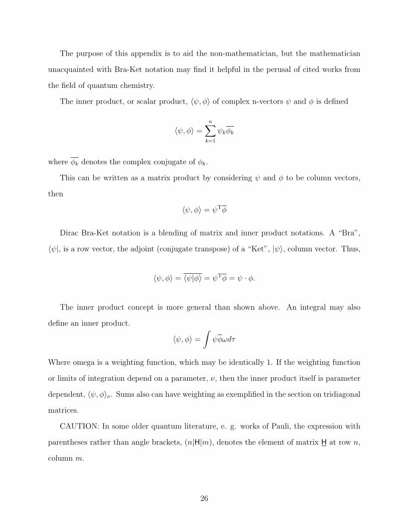
Throughout this work I shall prefer inner product notation, as above, to integral notation,

∂Eν

∂ν=

∫τψν

∂Hν

∂νψνdτ , and to Bra-Ket notation of Dirac, ∂Eν

∂ν= 〈ψν |∂Hν

∂ν|ψν〉 , both commonly

used in the literature of quantum physics and chemistry. See the appendix about notation.

4

Chapter 2

Statement and Proof

The Hellmann-Feynman theorem with one-dimensional variation is here stated with proof,

from Mourad E. H. Ismail and Ruiming Zhang [26].

Theorem: Let S be an inner product space with inner product 〈·, ·〉ν , possibly

depending on a parameter, ν ∈ I = (a, b). Let Hν be a symmetric operator on S

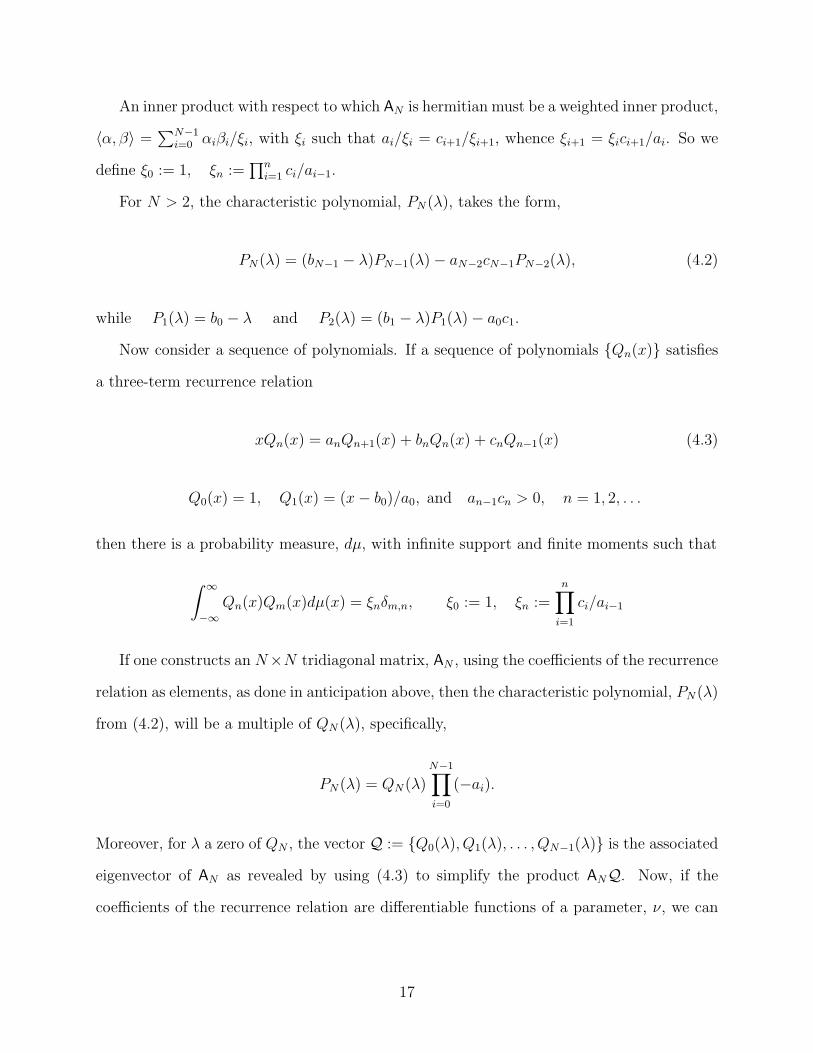
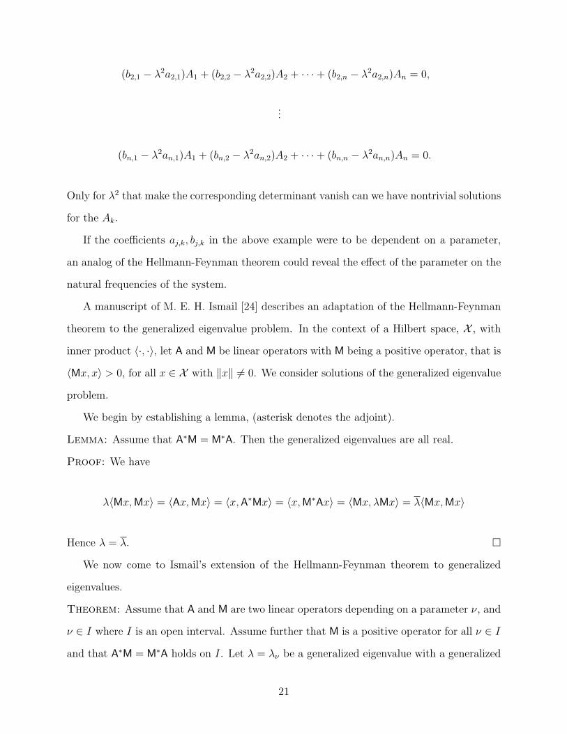
and assume that ψν is an eigenfunction of Hν corresponding to an eigenvalue λν .

Further assume that

limµ→ν

〈ψµ, ψν〉ν = 〈ψν , ψν〉ν > 0 (2.1)

and that

limµ→ν

⟨(Hµ − Hν

µ− ν

)ψµ, ψν

⟩ν

exists. (2.2)

If we define ∂Hν

∂νby

⟨∂Hν

∂νψν , ψν

⟩ν

:= limµ→ν

⟨(Hµ − Hν

µ− ν

)ψµ, ψν

⟩ν

(2.3)

then dλν/dν exists for ν ∈ (a, b) and is given by

dλνdν

=

⟨∂Hν

∂νψν , ψν

⟩ν

〈ψν , ψν〉ν(2.4)

5

Proof: Clearly, Hµψµ = λµψµ implies

〈Hµψµ, ψν〉ν = λµ〈ψµ, ψν〉ν .

Hence

(λµ − λν)〈ψµ, ψν〉ν = 〈Hµψµ, ψν〉ν − 〈ψµ,Hνψν〉ν . (2.5)

The symmetry of the operator Hν implies

(λµ − λν)〈ψµ, ψν〉ν = 〈(Hµ − Hν)ψµ, ψν〉ν . (2.6)

We now divide by µ− ν and then let µ→ ν in (2.6). The limit of the right-hand

side of (2.6) exists, for ν ∈ I, and equals

⟨∂Hν

∂νψν , ψν

⟩ν

(2.7)

while the second factor on the left side tends to the positive number 〈ψν , ψν〉ν as

µ→ ν, ν∈ I. Thus the limit of the remaining factor exists and (2.4) holds. This

completes the proof. �

The significance of the definition of the derivative of the operator, equation (2.3), warrants

emphasis. It is innovative and not equivalent to earlier usage, which was that of a Frechet

differential, defined by ∂Hν

∂ν= A such that

limh→0

supψ∈S

||Hν+h−Hν

hψ − Aψ||

||ψ||= 0

with concomitant questions of existence that the new definition avoids. Clearly, conformity

to the new definition in writing the derivative of the operator is required.

6

The theorem can readily be generalized for n-dimensional ν.

∇νλν = ∇ν 〈Hνψν , ψν〉ν =n∑k=1

⟨∂Hν

∂νkψν , ψν

⟩ν

νk (2.8)

where νk denotes the kth unit basis vector of ν. Recalling the origin of ν, realize that to

restore ν further amounts to dispensing with the Born-Oppenheimer approximation.

7

Chapter 3

The Quantum Chemistry Context

3.1 Electrostatic Theorem

“The electrostatic theorem” is an often-used alias for the Hellmann-Feynman theorem. Al-

though quantum chemists frequently employ the Hellmann-Feynman theorem, they often

have misconceptions about it. Many believe that it proves that the forces on the nuclei are

purely electrostatic forces. Rather, that is the premise for its application, not the conclusion.

While the notion that the theorem is obviously true is widely held, challenges to the validity

or reliability of the theorem also appear frequently. This is in part attributable to misunder-

standing of the theorem. But instability is a serious issue, as Slater has indicated, “. . . the

Hellmann-Feynman theorem has been less [useful]. The reason is that most molecular work

has been done with very inaccurate approximations to molecular orbitals.” Which is to say,

the approximations of ψ are often insufficiently accurate models of the physical system.

As an example of misunderstanding, the objection that the dependence of the operator

on a parameter does not guarantee that the eigenvalues and eigenfunctions will be smoothly

dependent on the parameter [31] overlooks the corresponding stated requirement, the eigen-

function must be continuous with respect to the parameter.

A second objection, that the derivative of the eigenfunction with respect to the pa-

8

rameter, ∂ψν

∂ν, may lie outside the domain of the operator [31], has its basis in a weak-

ness of earlier proofs, including Feynman’s, Hellmann’s and Guttinger’s, that they did ex-

press such a derivative and tacitly assumed its existence and the existence of the integral∫τ∂ψν

∂νHνψνdτ = Eν

∫τ∂ψν

∂νψνdτ . The arguments ran thus

∂Eν∂ν

=∂

∂ν〈Hνψν , ψν〉

=

⟨∂Hν

∂νψν , ψν

⟩+

⟨∂ψν∂ν

,Hνψν

⟩+

⟨Hνψν ,

∂ψν∂ν

⟩=

⟨∂Hν

∂νψν , ψν

⟩+ Eν

(⟨∂ψν∂ν

, ψν

⟩+

⟨ψν ,

∂ψν∂ν

⟩)

where the two rightmost terms are, by various rationales, together equated to zero. Most

commonly, as Eν∂∂ν〈ψν , ψν〉 = Eν

∂∂ν

(1), but Hellmann argued that the rightmost two terms

were separately zero for extremal Eν .

The importance of the continuity of ψν with respect to ν must not be overlooked. In

particular, degeneracy of eigenvalues gives rise to linear combinations of eigenfunctions that

are not continuously dependent on ν. In a condition of degeneracy the eigenfunctions for

which the Hellmann-Feynmann theorem holds are not well-defined. A method of handling

degeneracy has been described by S. Raj Vatsya [36] in terms of matrices. For an N -fold

degeneracy at ν = ν0, consider an arbitrary basis vector φn(ν0), n = 1, 2, . . . , N of the

degenerate eigenspace. Let PN(ν0) be the orthogonal projection matrix that projects an

arbitrary vector of the space onto the degenerate eigenspace. For for a perturbed ν 6= ν0, we

can write

H(ν)PN(ν) = E(ν)PN(ν)

with N distinct solutions for En(ν) and corresponding eigenvectors φn(ν). Differentiating

this, left multiplying by PN(ν) and evaluating the result at ν0 yields a matrix ON(ν0),

ON(ν0) = PN(ν0)∂H

∂ν(ν0)PN(ν0) =

∂E

∂ν(ν0)PN(ν0),

9

which has as eigenvalues the correct ∂En

∂ν(ν0) and corresponding eigenvectors of H(ν0).

The theorem does not guarantee stability. This is an important consideration in quantum

chemistry applications. The Born-Oppenheimer model is approximate; it is understood that

an actual molecule has oscillating nuclei. As data input, ν gives rise to error in ψν , Eν , and

∂Eν

∂ν. Stability improves as variation of ψν with respect to ν decreases. Andrew C. Hurley

has examined the question of stability of the eigenvalue approximations [22] [21]. Relying

on differentiability of the wave function, he establishes a criterion for assessing stability

and a procedure for minimizing instability. For the ground state of a stable molecular

configuration, the Born-Oppenheimer solution coincides with a local stability maximum by

Hurley’s criterion. Saul T. Epstein has confirmed the applicability of Hurley’s criterion for

stabilities of several Hellmann-Feynman variants including the integral version (below) and

a time-dependent version due to Edward F. Hayes and Robert G. Parr [7] [14].

3.2 Integral Hellmann-Feynman Theorem

An intermediate result in the proof of the Hellmann-Feynman theorem, equation (2.6) re-

produced here,

(λµ − λν)〈ψµ, ψν〉ν = 〈(Hµ − Hν)ψµ, ψν〉ν .

leads directly to corollary known as the integral Hellmann-Feynman theorem.

Corollary: If the conditions of the Hellmann-Feynman theorem are met, then

(λµ − λν) =〈(Hµ − Hν)ψµ, ψν〉ν

〈ψµ, ψν〉ν. (3.1)

This result, also known as Parr’s theorem, is useful for estimating molecular bond energies

[32].

10

3.3 Adiabatic, Virial and Hypervirial Theorems

The adiabatic theorem states that the evolving eigenstate of a slowly varying Hamiltonian

closely approximates at each instant the eigenstate that would exist if the Hamiltonian were

at that point unvarying. A slowly varying Hamiltonian is dependent on a time-parameter so

the Hellmann-Feynmann theorem can be applied. The work of Born and Fock [2], previously

cited as containing a precursor of the Hellmann-Feynman theorem, is acknowledged as a

significant proof of the adiabatic theorem. The histories of the two theorems involve many

of the same people. A recent work by Joseph E.Avron and Alexander Elgart [1] is an excellent

source of the history as well as providing the latest advance.

The virial theorem dates from the nineteenth century work of Rudolf Clausius. It states

that for a bound system governed by an inverse square law of attraction average kinetic has

half the magnitude of the average potential energy (taken to be zero at infinite separation).

It is said that the Hellmann-Feynman theorem can be used to provide an alternate proof

of the virial theorem. Allied theorems, as a group called hypervirial theorems, sometimes

parallel or coincide with variant forms of the Hellmann-Feynman theorem [8].

Allied to the Hellmann-Feynmann theorem, in the class of hypervirial theorems, there

exists an off-diagonal Hellmann-Feynman formula for the case of distinct eigenvalues, λm

and λn, of the operator at a single value of the parameter ν,

(λm − λn)

⟨ψn,

∂ψm∂ν

⟩=

⟨ψn,

∂H

∂νψm

⟩,

where ψm and ψn are eigenfunctions associated with the respective eigenvalues. A simple

derivation of the off-diagonal formula starts with

λmψm = Hψm.

11

Take the inner product with ψn and differentiate.

∂

∂ν〈ψn, λmψm〉 =

∂

∂ν〈ψn,Hψm〉 .

Provided that we can take the differentiation inside the inner product and that⟨ψn,H

∂ψm

∂ν

⟩and

⟨H∂ψm

∂ν, ψn

⟩make sense, we proceed,

∂λm∂ν

〈ψn, ψm〉+ λm

⟨ψn,

∂ψm∂ν

⟩+ λm

⟨∂ψn∂ν

, ψm

⟩

=

⟨∂ψn∂ν

,Hψm

⟩+

⟨Hψn,

∂ψm∂ν

⟩+

⟨ψn,

∂H

∂νψm

⟩,

where we have used the symmetry of the operator. Noting that the first term on the left

side is zero by the orthogonality of the eigenfunctions and that the last term on the left side

equals the first term on the right side, we simplify to the result,

(λm − λn)

⟨ψn,

∂ψm∂ν

⟩=

⟨ψn,

∂H

∂νψm

⟩.

This off-diagonal formula appears in the 1928 paper by Born and Fock [2] and is the

Hellmann-Feynman antecedent previously mentioned, see example (c) in figure 1.1. Condi-

tions under which this formula is said to hold are variously stated [5] [28] [9].

12

Chapter 4

The Variation of Zeros of Orthogonal

Polynomials

In 1977, a physicist, John T. Lewis, in collaboration with a mathematician, Martin E. Mul-

doon, published a demonstration of the applicability of the Hellmann-Feynman theorem to a

Sturm-Liouville operator and utilized the result to reveal monotonicity and convexity prop-

erties of the zeros of Bessel functions. Other mathematicians followed the lead in applying

the theorem to the study of special functions and orthogonal polynomials. By 1988 a new

technique of constructing tridiagonal matrix operators from three term recursion relations

had come into use.

4.1 Sturm-Liouville Operators

Lewis and Muldoon [29] stated and proved, as a lemma, an adaptation of the Hellmann-

Feynman theorem for the Sturm-Liouville problem,

[− d

dx

(p(x)

d

dx

)+ ν2q(x)

]ψ(x) = λφ(x)ψ(x), a < x ≤ b,

13

with boundary conditions

limx→a+

p(x)ψ(x)ψ′(x) = p(b)ψ(b)ψ′(b).

They used integral notation, normalizing ψ with the inner product

〈ψ, ψ〉 :=

∫ b

a

φψψdx = ‖ψ‖2 = 1.

The parameter dependent operator,

Lν :=1

φ

[− d

dx

(pd

dx

)+ ν2q

]

is symmetric for the given boundary conditions and inner product. Now, comparing the

effect of two values of the parameter, µ and ν, on the inner product 〈ψµ, ψν〉 we find

〈ψµ, (Lν − Lµ)ψν〉 = (λν − λµ)〈ψµ, ψν〉 = (ν2 − µ2)

∫ b

a

qψµψνdx

where we have dropped terms that integrate to zero. After dividing by ν − µ, the limit,

µ→ ν, yields the derivative,

dλνdν

=

⟨ψν ,

dLνdν

ψν

⟩= 2ν

∫ b

a

qψνψνdx,

which is the Hellmann-Feynman result.

Using the above result to rewrite the derivative ddν

λν

ν, Lewis and Muldoon found,

d

dν

λνν

=1

ν

dλνdν

− λνν2

= 2

∫ b

a

qψνψνdx−λνν2

=

∫ b

a

[2q − λνφ

ν2

]ψνψνdx

where in the last step the normalization has been used. Then applying that result to the

14

rewriting of ddν

λν

ν2 they obtained,

d

dν

λνν2

=1

ν

∫ b

a

[2q − λνφ

ν2

]ψνψνdx−

λνν3

∫ b

a

φψνψνdx

=−2

ν3

∫ b

a

[−ν2qdx+ λνφ

]ψνψνdx

= − 2

ν3

∫ b

a

ψν

[− d

dx

(p(x)

dψνdx

)]dx

= − 2

ν3

∫ b

a

p

(dψνdν

) (dψνdν

)dx

In the last steps they substitute from the original equation, integrate by parts and drop a

term that evaluates to zero by reason of the boundary conditions.

4.2 A Second Derivative Version

A second derivative version of the Hellmann-Feynman theorem appeared in an article by

Ismail and Muldoon [25].

First differentiate λνψν = Lνψν to obtain,

∂Lν∂ν

ψν = (λν − Lν)

(∂ψν∂ν

)+

(∂λν∂ν

)ψν (4.1)

If the definition of the inner product is independent of ν and ν is real, then the symmetry

of the operator Lν is inherited by its derivative, ∂Lν

∂ν. Using this in differentiating

∂λν∂ν

=

⟨ψν ,

∂Lν∂ν

ψν

⟩

one obtains

∂2λν∂ν2

=

⟨ψν ,

∂2Lν∂ν2

ψν

⟩+

⟨∂ψν∂ν

,∂Lν∂ν

ψν

⟩+

⟨∂Lν∂ν

ψν ,∂ψν∂ν

⟩

15

Substituting for ∂Lν

∂νψν from 4.1 the rightmost two terms become

⟨∂ψν∂ν

, (λν − Lν)∂ψν∂ν

+∂λν∂ν

ψν

⟩+

⟨(λν − Lν)

∂ψν∂ν

+∂λν∂ν

ψν ,∂ψν∂ν

⟩

=

⟨∂ψν∂ν

, (λν − Lν)∂ψν∂ν

⟩+

⟨(λν − Lν)

∂ψν∂ν

,∂ψν∂ν

⟩+∂λν∂ν

(⟨∂ψν∂ν

, ψν

⟩+

⟨ψν ,

∂ψν∂ν

⟩)Utilizing the hermiticity of (λν − Lν) and the normalization of ψν we simplify to the result

∂2λν∂ν2

=

⟨ψν ,

∂2Lν∂ν2

ψν

⟩+ 2

⟨(λν − Lν)

∂ψν∂ν

,∂ψν∂ν

⟩

This second derivative formula had appeared previously in the literature of quantum chem-

istry [6]. The second derivative formula depends on stronger assumptions than the first

derivative formula; namely, differentiability of ψν and boundedness of⟨∂ψν

∂ν, ∂ψν

∂ν

⟩.

The following section relates to another innovation in the Ismail-Muldoon article.

4.3 Tridiagonal Matrices

The article by Ismail and Muldoon [25] and a second article, by Ismail [23], that appeared

the previous year, describe a technique in the study of variation with respect to a parameter

of zeros of orthogonal polynomials. The technique brings together three-term recurrence

relations, tri-diagonal matrices and the Hellmann-Feynman theorem.

Let us examine some properties of tridiagonal matrices. Let AN be an N ×N tridiagonal

matrix.

AN =

b0 a0 0

c1 b1 a1

c2 b2. . .

. . . . . . aN−3

cN−2 bN−2 aN−2

0 cN−1 bN−1

16

An inner product with respect to which AN is hermitian must be a weighted inner product,

〈α, β〉 =∑N−1

i=0 αiβi/ξi, with ξi such that ai/ξi = ci+1/ξi+1, whence ξi+1 = ξici+1/ai. So we

define ξ0 := 1, ξn :=∏n

i=1 ci/ai−1.

For N > 2, the characteristic polynomial, PN(λ), takes the form,

PN(λ) = (bN−1 − λ)PN−1(λ)− aN−2cN−1PN−2(λ), (4.2)

while P1(λ) = b0 − λ and P2(λ) = (b1 − λ)P1(λ)− a0c1.

Now consider a sequence of polynomials. If a sequence of polynomials {Qn(x)} satisfies

a three-term recurrence relation

xQn(x) = anQn+1(x) + bnQn(x) + cnQn−1(x) (4.3)

Q0(x) = 1, Q1(x) = (x− b0)/a0, and an−1cn > 0, n = 1, 2, . . .

then there is a probability measure, dµ, with infinite support and finite moments such that

∫ ∞

−∞Qn(x)Qm(x)dµ(x) = ξnδm,n, ξ0 := 1, ξn :=

n∏i=1

ci/ai−1

If one constructs an N×N tridiagonal matrix, AN , using the coefficients of the recurrence

relation as elements, as done in anticipation above, then the characteristic polynomial, PN(λ)

from (4.2), will be a multiple of QN(λ), specifically,

PN(λ) = QN(λ)N−1∏i=0

(−ai).

Moreover, for λ a zero of QN , the vector Q := {Q0(λ), Q1(λ), . . . , QN−1(λ)} is the associated

eigenvector of AN as revealed by using (4.3) to simplify the product ANQ. Now, if the

coefficients of the recurrence relation are differentiable functions of a parameter, ν, we can

17

apply the Hellmann-Feynman theorem and find,

dλ

dν=

⟨(d

dνAN

)Q,Q

⟩ν

/〈Q,Q〉ν , (4.4)

where the indicated derivative is taken element wise. Importantly, this result does not require

differentiation of the eigenvector or the orthogonal polynomials.

This version of the Hellmann-Feynman theorem together with certain other easily dis-

cerned properties of the system of orthogonal polynomials makes a variety of inferences

possible. For example, birth and death process polynomials obey a recurrence relationship

with coefficients related by bn = −(an + cn), an > 0, and cn ≥ 0 for n ≥ 0, with cn = 0 only

for n = 0, the lead coefficient of Qn has the sign (−1)n, and the zeros of Qn lie between zero

and the largest zero Λ of QN , n < N . Applying (4.4),

dΛ

dν

N−1∑i=0

Q2i (Λ)/ξi =

N−1∑i=0

Qi(Λ)[−daidν

Qi+1(Λ)− dcidνQi−1(Λ) +

d(ai + ci)

dνQi(Λ)]/ξi,

reveals a correlation of variation of Λ and the variation of the coefficients. If the coefficients

an and cn are nonincreasing (nondecreasing) functions of ν, then so is Λ, the largest zero of

QN (for any choice of N .)

Analogous results are found for least zeros, and for other types of orthogonal polynomials,

e. g. random walk polynomials. The paper by Ismail and Muldoon addresses infinite

dimensional matrix cases.

18

Chapter 5

Generalized Eigenvalue Problems

In the generalized eigenvalue problem two operators separately transforming the same vector

(function) yield vectors (functions) that differ from one another only by a scalar multiple,

Ax = λMx.

The scalar multiple, λ, is called a generalized eigenvalue of the operator pair. In the matrix

operator context, λ satisfies the equation

det (A− λM) =

∣∣∣∣∣∣∣∣∣∣∣∣∣

a1,1 − λm1,1 a1,2 − λm1,2 · a1,n − λm1,n

a2,1 − λm2,1 a2,2 − λm2,2 · a2,n − λm2,n

· · · ·

an,1 − λmn,1 an,2 − λmn,2 · an,n − λmn,n

∣∣∣∣∣∣∣∣∣∣∣∣∣= 0.

An interesting case in which we might encounter a generalized eigenvalue problem is a

mechanical system with n degrees of freedom governed by the system of Lagrange equations

∂T

∂yk− d

dt

∂T

∂yk=∂U

∂yk, (5.1)

where T is kinetic energy and U is potential energy. Let us suppose we have a stable

19

equilibrium point, ∂U∂yk

= 0 at y1 = y2 = · · · = yn = 0, with U at a minimum. Since U is only

defined to within an additive constant, we take U = 0 at the equilibrium point. Our interest

is discovering the natural frequency of small oscillations about this equilibrium point. In

general,

T =n∑

j,k=1

aj,kyj yk (5.2)

where the coefficients aj,k might be functions of the coordinates y, but we can regard them

as constant for small oscillations. If we expand U in powers of the y, the first two terms are

zero and our series begins with the second degree term. For small oscillations we neglect

higher order terms and write

U =n∑

j,k=1

bj,kyjyk (5.3)

with the constant coefficients bj,k = ∂2U∂yj∂yk

. Substituting (5.2) and (5.3) into our system of

Lagrange equations (5.1), we now have,

a1,1y1 + a1,2y2 + · · ·+ a1,nyn + b1,1y1 + b1,1y1 + · · ·+ b1,1y1 = 0

a1,1y1 + a1,2y2 + · · ·+ a1,nyn + b1,1y1 + b1,1y1 + · · ·+ b1,1y1 = 0

...

a1,1y1 + a1,2y2 + · · ·+ a1,nyn + b1,1y1 + b1,1y1 + · · ·+ b1,1y1 = 0 (5.4)

The solution has the form of harmonic oscillations of fixed frequency and phase but different

amplitudes.

yk = Akcos(λt+ ω) (5.5)

Substituting (5.5) into (5.4) we see the generalized eigenvalue problem,

(b1,1 − λ2a1,1)A1 + (b1,2 − λ2a1,2)A2 + · · ·+ (b1,n − λ2a1,n)An = 0,

20

(b2,1 − λ2a2,1)A1 + (b2,2 − λ2a2,2)A2 + · · ·+ (b2,n − λ2a2,n)An = 0,

...

(bn,1 − λ2an,1)A1 + (bn,2 − λ2an,2)A2 + · · ·+ (bn,n − λ2an,n)An = 0.

Only for λ2 that make the corresponding determinant vanish can we have nontrivial solutions

for the Ak.

If the coefficients aj,k, bj,k in the above example were to be dependent on a parameter,

an analog of the Hellmann-Feynman theorem could reveal the effect of the parameter on the

natural frequencies of the system.

A manuscript of M. E. H. Ismail [24] describes an adaptation of the Hellmann-Feynman

theorem to the generalized eigenvalue problem. In the context of a Hilbert space, X , with

inner product 〈·, ·〉, let A and M be linear operators with M being a positive operator, that is

〈Mx, x〉 > 0, for all x ∈ X with ‖x‖ 6= 0. We consider solutions of the generalized eigenvalue

problem.

We begin by establishing a lemma, (asterisk denotes the adjoint).

Lemma: Assume that A∗M = M∗A. Then the generalized eigenvalues are all real.

Proof: We have

λ〈Mx,Mx〉 = 〈Ax,Mx〉 = 〈x,A∗Mx〉 = 〈x,M∗Ax〉 = 〈Mx, λMx〉 = λ〈Mx,Mx〉

Hence λ = λ. �

We now come to Ismail’s extension of the Hellmann-Feynman theorem to generalized

eigenvalues.

Theorem: Assume that A and M are two linear operators depending on a parameter ν, and

ν ∈ I where I is an open interval. Assume further that M is a positive operator for all ν ∈ I

and that A∗M = M∗A holds on I. Let λ = λν be a generalized eigenvalue with a generalized

21

eigenvector x(ν). Then

dλνdν

=

⟨[M∗ dA

dν− A∗ dM

dν

]x, x

⟩〈Mx,Mx〉

(5.6)

Proof: Normalize x by

〈Mx,Mx〉 = 1

Clearly

λν = 〈λνMx,Mx〉 = 〈Ax,Mx〉 (5.7)

By differentiating the above equality we obtain

dλνdν

=

⟨dA

dνx,Mx

⟩+

⟨Adx

dν,Mx

⟩+

⟨Ax,

dM

dνx

⟩+

⟨Ax,M

dx

dν

⟩=

⟨dA

dνx,Mx

⟩+

⟨dx

dν,A∗Mx

⟩+

⟨Ax,

dM

dνx

⟩+

⟨Ax,M

dx

dν

⟩

Observe that the condition A∗M = M∗A implies

⟨dx

dν,A∗Mx

⟩+

⟨Ax,M

dx

dν

⟩=

⟨dx

dν,M∗Ax

⟩+ λ

⟨Mx,M

dx

dν

⟩= λ

[⟨Mdx

dν,Mx

⟩+

⟨Mx,M

dx

dν

⟩]= −λ

[⟨dM

dνx,Mx

⟩+

⟨Mx,

dM

dνx

⟩]

where the last step used the result of differentiating (5.7). Thus

dλνdν

=

⟨dA

dνx,Mx

⟩+

⟨dM

dνx,Ax

⟩

which simplifies to the right-hand side of (5.6). �

The requirement that A∗M = M∗A is somewhat milder that requiring symmetry. Sym-

metry of both operators is sufficient to satisfy the condition.

22

Chapter 6

Conclusion

Although for some problems, particularly molecular force problems, 〈ψν , ∂Lν

∂νψν〉, may not be

simple to evaluate. Conceptually, the Hellmann-Feynman theorem is beautifully simple and

direct and it has the capacity to reveal general properties of the variation of eigenvalues with

respect to a parameter. However, it requires symmetry of the operator at the point where the

derivative of the eigenvalue is taken. As seen in the tridiagonal matrix example, hermiticity

at a point may possibly be achieved by specially crafting an inner product for the purpose.

The cost in simplicity and directness becomes prohibitive for less tractable cases. It seems

unlikely that completely general applicability can ever be achieved by a Hellmann-Feynman

analog. However, a search for further extensions of applicability to special cases may yet be

profitable.

The number of mathematicians who have taken an interest in the Hellmann-Feynman

theorem remains small. The number of quantum chemists who take a mathematical interest

in the theorem is also small. A few names recur frequently in searches for mathematically

interesting works about the Hellmann-Feynman theorem.

Over the years, there have been researchers who used the theorem under other names, or

unnamed, and who were perhaps unaware of the designation “Hellmann-Feynman theorem”,

for example, physicist Gregory Breit [4] writing on scattering theory, used two forms of

23

the theorem without name or attribution. Others who might be expected to be aware of

the theorem seem not to have known of it by any name; Perturbation Theory for Linear

Operators by Tosio Kato [27], for example, makes no mention of the theorem. Improving

communication between disciplines might accelerate advances for all.

24

APPENDIX: ABOUT NOTATION

25

The purpose of this appendix is to aid the non-mathematician, but the mathematician

unacquainted with Bra-Ket notation may find it helpful in the perusal of cited works from

the field of quantum chemistry.

The inner product, or scalar product, 〈ψ, φ〉 of complex n-vectors ψ and φ is defined

〈ψ, φ〉 =n∑k=1

ψkφk

where φk denotes the complex conjugate of φk.

This can be written as a matrix product by considering ψ and φ to be column vectors,

then

〈ψ, φ〉 = ψTφ

Dirac Bra-Ket notation is a blending of matrix and inner product notations. A “Bra”,

〈ψ|, is a row vector, the adjoint (conjugate transpose) of a “Ket”, |ψ〉, column vector. Thus,

〈ψ, φ〉 = 〈ψ|φ〉 = ψTφ = ψ · φ.

The inner product concept is more general than shown above. An integral may also

define an inner product.

〈ψ, φ〉 =

∫ψφωdτ

Where omega is a weighting function, which may be identically 1. If the weighting function

or limits of integration depend on a parameter, ν, then the inner product itself is parameter

dependent, 〈ψ, φ〉ν . Sums also can have weighting as exemplified in the section on tridiagonal

matrices.

CAUTION: In some older quantum literature, e. g. works of Pauli, the expression with

parentheses rather than angle brackets, (n|H|m), denotes the element of matrix H at row n,

column m.

26

LIST OF REFERENCES

[1] J. E. Avron and A. Elgart. Adiabatic Theorm without a Gap Condition. Com-

mun.Math.Phys., 203:445–463, 1999.

[2] M. Born and V. Fock. Proof of the Adiabatic Theorem. Z. Phys., 51:165–169, 1928.

[3] M. Born and J. R. Oppenheimer. Zur Quantentheorie der Molekeln. Ann. Physik,

84(20):457–484, 1927.

[4] G. Breit. Topics in Scattering Theory. Rev. Mod. Phys., 23(3):238–252, 1951.

[5] E. A. Castro and F. M. Fernandez. Comment on the Off-Diagonal Hellmann-Feynman

Formula. J. Chem. Phys., 73(9):4711, 1980.

[6] B. M. Deb. Note on an Upper Bound Property of Second Derivatives of the Energy.

Chem. Phys. Lett., 17(1):78–79, 1972.

[7] S. T. Epstein. Time-Dependent Hellmann-Feynman Theorems for Variational Wave-

functions. J. Chem. Phys., 45(1):384, 1966.

[8] S. T. Epstein. The Variation Method in Quantum Chemistry. Academic Press, 1974.

[9] S. T. Epstein and J. O. Hirschfelder. Hypervirial Theorems for Variational Wave Func-

tions. Phys. Rev., 123(4):1495–1502, 1961.

[10] W. H. E. Schwarz et al. Hans G. A. Hellmann (1903–1938), part I. Bunsenmagazin,

1(1):60–70, 1999.

27

[11] W. H. E. Schwarz et al. Hans G. A. Hellmann (1903–1938), part II. Bunsenmagazin,

1(2):10–21, 1999.

[12] R. P. Feynman. Forces in Molecules. Phys. Rev., 56(4):340–343, 1939.

[13] P. Guttinger. Das Verhalten von Atomen im magnetischen Drehfeld. Z. Phys., 73:169–

184, 1931.

[14] E. F. Hayes and R. G. Parr. Time-Dependent Hellmann-Feynman Theorems. J. Chem.

Phys., 43(5):1831–1832, 1965.

[15] H. G. A. Hellmann. Zur rolle der kinetischen Elektronenenergie fur die zweischen-

atomaren Krafte. Z Phys, 85:180–190, 1933.

[16] H. G. A. Hellmann. A New Approximation Method in the Problem of Many Electrons.

J. Chem. Phys., 3:61, 1935.

[17] H. G. A. Hellmann. Contributed Discussions to: F. London. The General Theory of

Molecular Forces. Trans. Faraday Soc., 33:40–42,278–279, 1937.

[18] H. G. A. Hellmann. Einfuhrung in die Quantenchemie. Deuticke, Leipzig, 1937.

[19] H. G. A. Hellmann. Quantum Chemistry. [Russian]. ONTI, Moscow, 1937.

[20] H. G. A. Hellmann. Einfuhrung in die Quantenchemie. J. W. Edwards, Ann Arbor,

Michigan, 1944.

[21] A. C. Hurley. The Electrostatic Calculation of Molecular Energies. II. Approxi-

mate Wave Functions and the Electrostatic Method. Proc. Roy. Soc. (London),

226(1165):179–192, 1954.

[22] A. C. Hurley. Introduction to the Electron Theory of Small Molecules. Academic Press,

1976.

28

[23] M. E. H. Ismail. The Variation of Zeros of certain Orthogonal Polynomials. Adv. Applied

Math., 8(1):111–118, 1987.

[24] M. E. H. Ismail. Monotonicity of Zeros of Biorthogonal Rational Functions. unpublished

manuscript, 2003.

[25] M. E. H. Ismail and M. E. Muldoon. On the Variation with respect to a Parameter of

Zeros of Bessel and q-Bessel Functions. J. Math. Anal. Appl., 135(1):187–207, 1988.

[26] M. E. H. Ismail and R. Zhang. The Hellmann-Feynman Theorem and the Variation

of Zeros of Special Functions. In N. K. Thakare, editor, Ramanujan International

Symposium on Analysis, pages 151–183, Delhi, 1989. Macmillan India.

[27] T. Kato. Perturbation Theory for Linear Operators. Springer-Verlag, 1966.

[28] D. J. Klein and P. L. DeVries. Satisfying certain Matrix Element Formulas. J. Chem.

Phys., 68(1):160–162, 1978.

[29] J. T. Lewis and M. E. Muldoon. Monotonicity and Convexity Properties of Zeros of

Bessel Functions. SIAM J. Math. Anal., 8(1):171–178, 1977.

[30] W. Pauli. Uber das Modell des Wasserstoffmolekulions. Ann. Physik, 68:177–240, 1922.

[31] V. I. Pupyshev. The Nontriviality of the Hellmann-Feynman Theorem. Russian J. Phys.

Chem., 74:S267–S278, 2000.

[32] R. E. Wyatt S. T. Epstein, A. C. Hurley and R. G. Parr. Integrated and Integral

Hellmann-Feynman Formulas. J. Chem. Phys., 47(4):1275–1286, 1967.

[33] E. Schrodinger. Quantisierung als Eigenwertproblem. Ann. Physik, 79:361–379, 1926.

[34] J. C. Slater. Solid State and Molecular Theory. Wiley, 1975.

[35] A. L. Tchougreeff. Introduction. Int. J. Q. Chem., 88(4):357, 2002.

29

[36] S. R. Vatsya. Comment on Breakdown of the Hellmann-Feynman Theorem: Degeneracy

is the Key. Phys. Rev. B, 69:037102, 2004.

30