Weibel’s homological algebra is a text with a lot of content but also a lot left to the reader.This document is intended to cover what’s left to the reader: I try to fill in gaps in proofs,perform checks, make corrections, and do the exercises. It is very much in progress, coveringonly chapters 3 and 4 at the moment.
I will assume roughly the same pre-requisites as Weibel: knowledge of some categorytheory and graduate courses in algebra covering modules, tensor products, and localizationsof rings. I will assume less mathematical maturity.
2. Missing Details
2.1. Chapter 1.
2.1.1. Section 1.6.
Example 1.6.8. It is not quite true that AUop = Presheaves(X), since there are functorsthat do not take the empty set to 0. In fact, some sources do not require that presheavestake the empty set to zero. With or without this requirement, the resulting category ofpresheaves is an abelian category.
2.2. Chapter 2.
2.2.1. Section 2.1.
2.2.2. Section 2.2.
2.2.3. Section 2.3.
2.2.4. Section 2.4.
Theorem 2.4.6. It is asserted that the image of a split exact sequence under an additivefunctor is exact. See Theorem 4 in “Additional Math” below for a (lengthy, but I thinkneat) proof.
2.3. Chapter 3.
2.3.1. Section 3.1.
Proposition 3.1.2. This is the way that a group is a direct limit of its finitely generatedsubgroups. Let A be an abelian group.
First, we set up a diagram D whose objects are the finitely generated subgroups of A, andwhose arrows are the inclusion maps ϕ : G → H whenever G ≤ H for finitely generatedsubgroups G,H of A. This diagram is indexed by a filtered category, since for any pair G,Hof finitely generated subgroups of A, GH is also a finitely generated group, so G → GHand H → GH are arrows in the diagram (i.e. we satisfy axiom 1 of a filtered categoryin Definition 2.6.13) and there are no parallel arrows (i.e. we satisfy axiom 2 of a filteredcategory vacuously.)
The claim is that the colimit of this diagram is A. To see this, first of all, we have a mapϕG : G→ A for each f.g. subgroup G defined by the inclusion of G into A. This commuteswith all maps in the diagram since the inclusion of G into H followed by the inclusion of Hinto A is just the inclusion of G into A.
SOLUTIONS AND ELABORATIONS 3
It remains to show that A is a universal. Select another family of maps D → B. We willdefine a map ψ : A→ B commuting with everything. Let g ∈ A. The element g is containedin some f.g. subgroup G of A. We define ψ(g) to be the image of g under the map G→ B.This is the only way to define ψ so that
G
�� ��A
ψ // B
commutes, so if ψ defines a map that commutes with the maps D → A and D → B, it isunique. On the other hand, if H is another f.g. subgroup of A containing g, then since
G //
!!
GH
��
Hoo
}}B
commutes, the image of g under H → B must be the same as its image under the mapG → B. This shows that ψ is well defined. Finally, ψ is a group homomorphism, sincefor any g, h ∈ A, we may select a f.g. subgroup G so that g, h ∈ G. Let ϕ be the mapG→ B. Then ψ(g+h) = ϕ(g+h) = ϕ(g) +ϕ(h) = ψ(g) +ψ(h) since ϕ : G→ B is a grouphomomorphism. So there exists a unique group homomorphism A → B so that everythingcommutes, as desired, and A is the colimit.
Intuitively, the direct limit is a fancy way to express a union, and of course A is a unionof its finitely generated subgroups, since each element of A is contained in some finitelygenerated subgroup. The argument above shows that the formal definition agrees with thisintuition.
Proposition 3.1.4. The reason that TorZn(Zm, B) = 0 is that Zm is a free Z-module, henceprojective, and Tor vanishes on projective modules.
2.3.2. Section 3.2.
Definition 3.2.1. The target category of − ⊗R B is intended to be Ab. If B is an R-Sbimodule, we can also view − ⊗R B as a functor from mod-R to mod-S. Again, this isalways right exact. It is equivalent for − ⊗ B to be exact as a functor to Ab and as afunctor to mod-S, since in each case exactness is the same as taking every injection A′ → Aof R-modules to an injective map A′ ⊗ B → A ⊗ B: we just view the map as a grouphomomorphism if Ab is the target and as an S-module homomorphism if mod-S is thetarget. This means that flatness of B does not depend on which category we take to be thetarget of −⊗R B, although it does depend on R.
Theorem 3.2.2. For an alternate proof without colimits, see [2, Proposition 2.5].We show that the colimit indicated in the text is the localization, as claimed. Our tech-
nique will be to use an explicit description of filtered colimits. Namely, if I is a filteredcategory, and F : I → R-mod is an additive functor, the colimit of F is the module Cwhose additive group has underlying set
C =
(⊔i∈I
F (i)
)/ ∼
4 SEBASTIAN BOZLEE
where a ∈ F (i) and b ∈ F (j) are equivalent a ∼ b if there exist arrows ϕ : i → k andψ : j → k so that F (ϕ)(a) = F (ψ)(b). The addition of a ∈ F (i) and b ∈ F (j) is definedby taking a pair of arrows ϕ : i → k and ψ : j → k (whose existence is assured since I is afiltered category) and letting a + b be the sum F (ϕ)(a) + F (ψ)(b) in k. For r ∈ R we takethe scalar product of r and a ∈ F (i) to be ra ∈ F (i).
In our particular case, a ∈ F (s1) and b ∈ F (s2) are equivalent if and only if there existsa number c ∈ S so that cs2a = cs1b. Next, note that a ∼ b if and only if a
s1= b
s2in S−1R.
Therefore the map ϕ : C → S−1R defined by a ∈ F (s1) 7→ as1
is a well defined bijection.
Next, the sum of a ∈ F (s1) and b ∈ F (s2) is s2a + s1b ∈ F (s1s2), so ϕ preserves addition.Finally, the scalar product of r ∈ R and a ∈ F (s1) is ra ∈ F (s1), so ϕ preserves scalarmultiples. Altogether, the colimit C is isomorphic to the localization S−1R, as claimed.
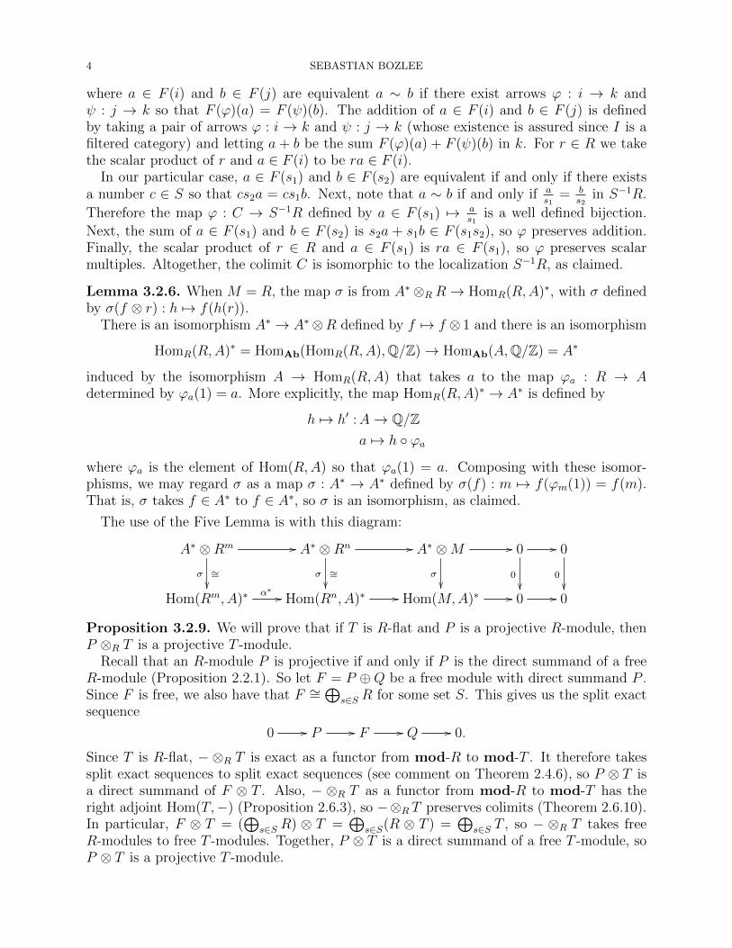
Lemma 3.2.6. When M = R, the map σ is from A∗⊗R R→ HomR(R,A)∗, with σ definedby σ(f ⊗ r) : h 7→ f(h(r)).
There is an isomorphism A∗ → A∗⊗R defined by f 7→ f ⊗ 1 and there is an isomorphism
induced by the isomorphism A → HomR(R,A) that takes a to the map ϕa : R → Adetermined by ϕa(1) = a. More explicitly, the map HomR(R,A)∗ → A∗ is defined by
h 7→ h′ :A→ Q/Za 7→ h ◦ ϕa
where ϕa is the element of Hom(R,A) so that ϕa(1) = a. Composing with these isomor-phisms, we may regard σ as a map σ : A∗ → A∗ defined by σ(f) : m 7→ f(ϕm(1)) = f(m).That is, σ takes f ∈ A∗ to f ∈ A∗, so σ is an isomorphism, as claimed.
Proposition 3.2.9. We will prove that if T is R-flat and P is a projective R-module, thenP ⊗R T is a projective T -module.
Recall that an R-module P is projective if and only if P is the direct summand of a freeR-module (Proposition 2.2.1). So let F = P ⊕Q be a free module with direct summand P .Since F is free, we also have that F ∼=
⊕s∈S R for some set S. This gives us the split exact
sequence
0 // P // F // Q // 0.
Since T is R-flat, − ⊗R T is exact as a functor from mod-R to mod-T . It therefore takessplit exact sequences to split exact sequences (see comment on Theorem 2.4.6), so P ⊗ T isa direct summand of F ⊗ T . Also, − ⊗R T as a functor from mod-R to mod-T has theright adjoint Hom(T,−) (Proposition 2.6.3), so −⊗R T preserves colimits (Theorem 2.6.10).In particular, F ⊗ T = (
⊕s∈S R) ⊗ T =
⊕s∈S(R ⊗ T ) =
⊕s∈S T , so − ⊗R T takes free
R-modules to free T -modules. Together, P ⊗ T is a direct summand of a free T -module, soP ⊗ T is a projective T -module.
SOLUTIONS AND ELABORATIONS 5
Lemma 3.2.11. To see why we require that r is central, let µi : Pi → Pi be the map p 7→ rp.Then µi is an R-module homomorphism if and only if for all s ∈ R, p ∈ P
srp = sµ(p) = µ(sp) = rsp.
This holds with no conditions on Pi if sr = rs for all s ∈ R, that is, if r is central. Had wenot required that r were central, we would then have to impose conditions on the projectiveresolution P → A to maintain that µ : P → P is a chain map.
Corollary 3.2.13. The equality Rp ⊗RM = TorRpn (Ap, Bp) follows by first noting
Rp ⊗RM = Rp ⊗R TorRn (A,B) = TorRpn (A⊗R Rp, Rp ⊗R B)
from Corollary 3.2.10, and then using that A⊗Rp and Rp⊗B are equal to the localizationsof A and B at p, respectively.
2.3.3. Section 3.3.
Example 3.3.3. Ext0Z(A,Z) is zero since we have assumed that A is a torsion group: torsion
elements must be sent to torsion elements, so the only homomorphism A → Z is the zerohomomorphism.
The comment that Ext1Z(Zp∞ ,Z) = lim←−(Z/pn) is proved in Application 3.5.10.
Example 3.3.5.
(1) This is because A ∼=⊕∞
i=1 Z/p, so
Ext1Z/m(A,Z/p) =
∞∏i=1
Ext1Z/m(Z/p,Z/p) =
∞∏i=1
Z/p.
where the first equality follows from Proposition 3.3.4 part 1 and the second followsfrom Exercise 3.3.2. The last is a vector space of uncountably infinite dimension.
(2) The displayed equation follows from Proposition 3.3.4 part 2 and Calculation 3.3.2.(Ext1
Z is intended.) The comment on divisibility follows since A is divisible if andonly if A = pA for all p ≥ 2 if and only if A/pA = 0 for all p ≥ 2.
Heuristically, there seems to be a duality between being torsionfree and divisible.TorZ1 (−,Q/Z) tests for torsion and Ext1
Z(−,∏∞
p=2 Z/p) tests for divisibility.
Lemma 3.3.6. Weibel asserts that HomAb(A,B) is a (left) R-module when R is commuta-tive. Here is why. We define rf : A→ B for r ∈ R and f ∈ HomAb(A,B) by (rf)(b) = f(rb).In order for this action to make HomAb(A,B) an R-module, we need rf to be an R-modulehomomorphism for all r. Now rf is an R-module homomorphism if and only if for all s ∈ Rand b ∈ B,
f(srb) = sf(rb) = s(rf)(b) = (rf)(sb) = f(rsb).
If we assume R is commutative, then srb = rsb, so we get the equality above for free.Otherwise, we would have to impose conditions on A and B to maintain that HomAb(A,B)is an R-module.
The assertion that multiplication by r gives a chain map when r is central is addressed inmy comment on Lemma 3.2.11.
Lemma 3.3.8. Let’s check the isomorphism for A = R. Then
S−1HomR(A,B) = S−1HomR(R,B) ∼= S−1B.
6 SEBASTIAN BOZLEE
On the other hand,
HomS−1R(S−1A, S−1B) ∼= S−1B.
So both are equal to S−1B as R-modules, as promised.The implication that the same holds for Rm is due to the fact that additive functors
preserve direct sums. This is a corollary of Theorem 4 and Proposition 3 in “AdditionalMath” above.
2.3.4. Section 3.4.
Theorem 3.4.3. According to the errata, the theorem should be stated with Θ : ξ 7→ ∂(idB),instead of idA. We will see why as we fill in the details of this proof.
When Weibel writes that X → A is the map induced by the maps B0→ A and P → A,
he is referring to the universal property of pushouts: since
Mj //
�
P
��B
0 // A
commutes (we get zero when composing M → P → A by exactness of 0→M → P → A→0) there is a unique map X → A so that the following diagram commutes:
(1) Mj //
�
P
σ�� ϕ
��
Bi //
0 ++
Xϕ′
A
That map is the map we are to use in the sequence 0→ B → X → A→ 0. More explicitly, if
ϕ is the map Pϕ→ A, then the dotted map, ϕ′ : X → A, is defined by taking the equivalence
class of (p, b) in X to the element ϕ(p) in A. This is well defined since if (p, b) and (p′, b′)are two representatives of the same element of X, then ϕ(p)− ϕ(p′) = ϕ(p− p′) = ϕ(j(m))
for some m ∈M . By exactness of 0→Mj→ P
ϕ→ A→ 0, ϕ(j(m)) = 0.
Now we show that the bottom row of the diagram
(2) 0 // Mj //
�
Pϕ //
σ��
A // 0
0 // Bi // X
ϕ′ // A // 0
is exact. (The left square commutes by definition of pushout. The right square commutessince the right triangle of (1) commutes.)
Since ϕ is surjective, and ϕ = ϕ′ ◦σ, it follows ϕ′ is surjective. This shows exactness at A.The map i : B → X is defined by b 7→ [(0, b)]. Suppose that [(0, b)] = [(0, 0)]. Then, by
the definition of X, (0, b) = (0, 0) + (j(m),−β(m)) for some m ∈M . Since j is injective, wemust have that m = 0, so [(0, b)] = [(0, 0)]. Therefore i is injective. This shows exactness atB.
SOLUTIONS AND ELABORATIONS 7
Finally, suppose (p, b) is the equivalence class of some element of the kernel of ϕ′. Thenϕ(p) = 0, so by exactness of the first row, p = j(m) for some m ∈ M . Therefore, [(p, b)] =[(j(m), b)] = [(0, b+β(m))] is in the image of i. This shows exactness at X, and we are done.
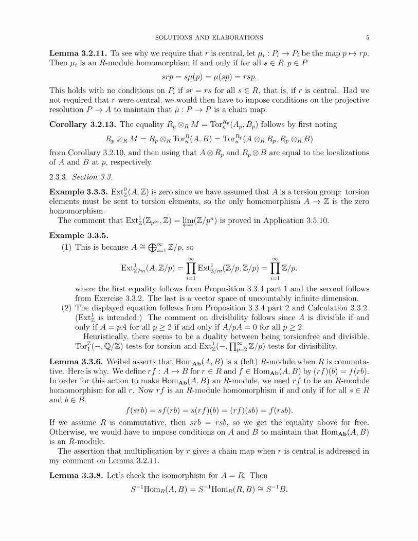
The reference to naturality of ∂ refers to the fact that this diagram, induced from the mor-phism of short exact sequences (2) by the contravariant cohomological δ-functor Ext∗(−, B),commutes:
Hom(M,B)∂ // Ext1(A,B)
Hom(B,B)
β∗
OO
∂ // Ext1(A,B)
id
OO
By commutativity of the diagram, ∂(idB) = ∂(β∗(idB)) = ∂(β) = x. This gives surjectivityof Θ.
Now we will check that the maps i : B → X and σ+ i◦f : P → X induce an isomorphismX ′ ∼= X and an equivalence between ξ′ and ξ. Recall that we have picked two lifts, β and β′
of some element x ∈ Ext1(A,B) under the map ∂ in the diagram
Hom(P,B)j∗ // Hom(M,B)
∂ // Ext1(A,B) // 0,
which we arrived at by taking the long exact sequence associated to 0→M → P → A→ 0under Ext∗(−, B). By exactness, the maps β and β′ differ by an element of the image of j∗,so we write β′ = β + f ◦ j, where f : P → B.
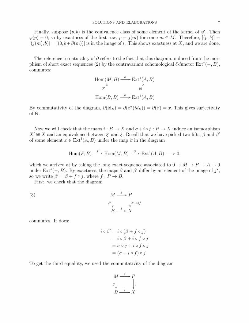
First, we check that the diagram
(3) Mj //
β′
��
P
σ+i◦f��
Bi // X
commutes. It does:
i ◦ β′ = i ◦ (β + f ◦ j)= i ◦ β + i ◦ f ◦ j= σ ◦ j + i ◦ f ◦ j= (σ + i ◦ f) ◦ j.
To get the third equaliity, we used the commutativity of the diagram
Mj //
�
P
σ��
Bi // X
8 SEBASTIAN BOZLEE
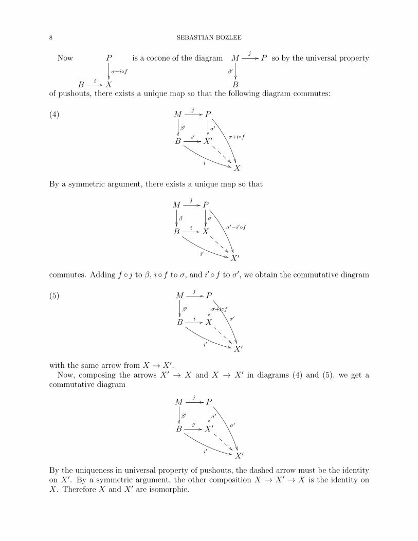
Now P
σ+i◦f��
Bi // X
is a cocone of the diagram Mj //
β′
��
P
B
so by the universal property
of pushouts, there exists a unique map so that the following diagram commutes:
(4) Mj //
β′
��
P
σ′��
σ+i◦f
��
Bi′ //
i ++
X ′
X
By a symmetric argument, there exists a unique map so that
Mj //
�
P
σ��
σ′−i′◦f
��
Bi //
i′ ++
X
X ′
commutes. Adding f ◦ j to β, i◦f to σ, and i′ ◦f to σ′, we obtain the commutative diagram
(5) Mj //
β′
��
P
σ+i◦f��
σ′
��
Bi //
i′ ++
X
X ′
with the same arrow from X → X ′.Now, composing the arrows X ′ → X and X → X ′ in diagrams (4) and (5), we get a
commutative diagram
Mj //
β′
��
P
σ′��
σ′
��
Bi′ //
i′ ++
X ′
!!X ′
By the uniqueness in universal property of pushouts, the dashed arrow must be the identityon X ′. By a symmetric argument, the other composition X → X ′ → X is the identity onX. Therefore X and X ′ are isomorphic.
SOLUTIONS AND ELABORATIONS 9
Finally, we show that the isomorphism X ′ → X induces an equivalence of extensions.Consider the diagram
ξ′ : 0 // Bi′ // X ′ //
��
A // 0
ξ : 0 // Bi // X // A // 0
where the middle arrow is the isomorphism X ′ → X. The left square commutes since thethe lower triangle of (4) commutes. The right square commutes because the right squares of
0 // Mj //
�
Pϕ //
σ��
A // 0
0 // Bi // X // A // 0
and
0 // Mj //
β′
��
Pϕ //
σ′
��
A // 0
0 // Bi′ // X // A // 0
commute. Therefore, ξ and ξ′ are equivalent extensions, as claimed.
Definition 3.4.4. I think it is helpful to compute the Baer sum of a simple example. Letus take the Baer sum of the extensions
ξ : 0 // Z/pp // Z/p2 1 // Z/p // 0,
ξ′ : 0 // Z/pp // Z/p2 2 // Z/p // 0.
Now the pullback X ′′ of Z/p2 1→ Z/p and Z/p2 2→ Z/p is the submodule {(x, y) ∈ Z/p2 ×Z/p2 | x ≡ 2y (mod p)} of Z/p2 × Z/p2. The pullback diagram is
X ′′π2 //
π1��
Z/p2
2��
Z/p2 1 // Z/p
We let Y be X ′′/{(px,−px) | x ∈ Z/p}. Then the Baer sum of ξ and ξ′is the sequence
0 // Z/pf // Y
g // Z/p // 0
where f takes x to [(px, 0)] = [(0, px)] and g takes [(x, y)] to x (mod p) or equivalently to2y (mod p).
10 SEBASTIAN BOZLEE
If p 6= 3, this is equivalent with the extension associated to i = 23
(mod p), via the followingequivalence:
0 // Z/pf // Y
g //
σ��
Z/p // 0
0 // Z/pp // Z/p2
23 // Z/p // 0
where σ : [(x, y)] 7→ x + y (mod p2). This is well defined, since any other representative of(x, y) is of the form (x− pz, y+ pz), and (x− pz, y+ pz) 7→ (x− pz) + y+ pz = x+ y. To see
that the bottom right map is 23, i.e. multiplication by 2 · 3−1 (mod p), note that (2, 1)
g7→ 2,
while (2, 1)σ7→ 3 (mod p2), and a morphism between cyclic groups must be multiplication
by some number.
Corollary 3.4.5. When Weibel refers to using the notation of the previous theorem, hemeans that we have constructed the following diagrams from the extensions ξ and ξ′:
(6) 0 // Mj //
γ
��
P //
τ��
A // 0
ξ : 0 // Bi // X // A // 0
and
(7) 0 // Mj //
γ′
��
P //
τ ′
��
A // 0
ξ′ : 0 // Bi′ // X ′ // A // 0.
We construct them by first using the lifting property of the projective module P to obtaina map τ : P → X and a map τ ′ : P → X ′. Then by commutativity of the right squares,τ(j(M)) ⊆ ker{X → A} and τ ′(j(M)) ⊆ ker{X ′ → A}. The exactness of the bottom rowsallows us to lift τ and τ ′ to maps γ = i−1 ◦ τ ◦ j and γ′ = (i′)−1 ◦ τ ◦ j respectively.
Recall that X ′′ is the pullback of the diagram
X ′′ //
��
X
��X ′ // A.
Now
Pτ //
τ ′��
X
��X ′ // A
SOLUTIONS AND ELABORATIONS 11
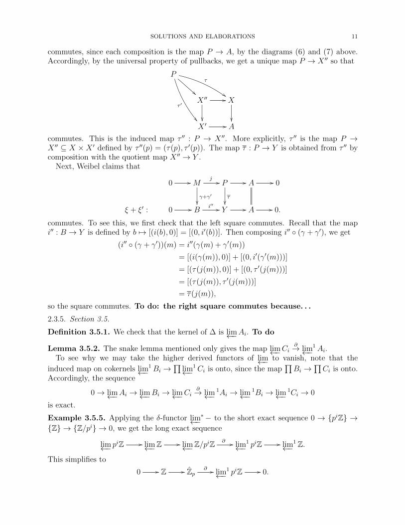
commutes, since each composition is the map P → A, by the diagrams (6) and (7) above.Accordingly, by the universal property of pullbacks, we get a unique map P → X ′′ so that
P
τ
$$
τ ′
��
X ′′ //
��
X
��X ′ // A
commutes. This is the induced map τ ′′ : P → X ′′. More explicitly, τ ′′ is the map P →X ′′ ⊆ X ×X ′ defined by τ ′′(p) = (τ(p), τ ′(p)). The map τ : P → Y is obtained from τ ′′ bycomposition with the quotient map X ′′ → Y .
Next, Weibel claims that
0 // Mj //
γ+γ′
��
P //
τ��
A // 0
ξ + ξ′ : 0 // Bi′′ // Y // A // 0.
commutes. To see this, we first check that the left square commutes. Recall that the mapi′′ : B → Y is defined by b 7→ [(i(b), 0)] = [(0, i′(b))]. Then composing i′′ ◦ (γ + γ′), we get
(i′′ ◦ (γ + γ′))(m) = i′′(γ(m) + γ′(m))
= [(i(γ(m)), 0)] + [(0, i′(γ′(m)))]
= [(τ(j(m)), 0)] + [(0, τ ′(j(m)))]
= [(τ(j(m)), τ ′(j(m)))]
= τ(j(m)),
so the square commutes. To do: the right square commutes because. . .
2.3.5. Section 3.5.
Definition 3.5.1. We check that the kernel of ∆ is lim←−Ai. To do
Lemma 3.5.2. The snake lemma mentioned only gives the map lim←−Ci∂→ lim←−
1Ai.To see why we may take the higher derived functors of lim←− to vanish, note that the
induced map on cokernels lim←−1Bi →
∏lim←−
1Ci is onto, since the map∏Bi →
∏Ci is onto.
Accordingly, the sequence
0→ lim←−Ai → lim←−Bi → lim←−Ci∂→ lim←−
1Ai → lim←−1Bi → lim←−
1Ci → 0
is exact.
Example 3.5.5. Applying the δ-functor lim←−∗− to the short exact sequence 0 → {piZ} →
{Z} → {Z/pi} → 0, we get the long exact sequence
lim←− piZ // lim←−Z // lim←−Z/piZ ∂ // lim←−
1 piZ // lim←−1 Z.
This simplifies to
0 // Z // Zp∂ // lim←−
1 piZ // 0.
12 SEBASTIAN BOZLEE
To see this, note that since each map piZ → pi−1Z is an inclusion, lim←− piZ =
⋂i p
iZ = 0.
It is clear that lim←−Z = Z. Finally, lim←−1 Z = 0 by Lemma 3.5.3. By exactness, we conclude
that lim←−1 piZ = Zp/Z. (To do: explain why the image of Z is the usual subgroup
identified with Z?)
Theorem 3.5.8. It is helpful to know that C = lim←−Ci is the complex whose jth degree
component is Cj = lim←−i
Ci,j and whose differentials Cjd→ Cj−1 are induced by the collection
of maps Ci,jd(i)→ Ci,j−1. (To do? Prove this statement.)
We apply the left exact functor lim←− to 0→ {Zi} → {Ci}d→ {Ci[−1]}, and obtain that
0→ lim←−Zi → Cd→ C[−1]
is exact. The last map is that induced by the collection of maps d(i) : Ci,j → Ci,j−1, so itsmaps in each degree are the differentials of C. Then by exactness, the degree j part of lim←−Ziis the kernel of the degree j part of C
d→ C[−1], so it really consists of the cycles of C, asclaimed.
Next, from the exact sequence 0→ {Zi} → {Ci}d→ {Bi[−1]} → 0, we get the long exact
sequence
0 // Z // Cd // lim←−Bi[−1] // lim←−
1 Zi // 0 // lim←−1Bi[−1] // 0
where we have lim←−1Ci = 0 by the Mittag-Leffler condition. By exactness, lim←−
1Bi[−1] = 0,
so the same holds of its shift, lim←−1Bi = 0, as claimed. Also by exactness, the kernel of
lim←−1Bi[−1] → lim←−
1 Zi is the image of Cd→ lim←−Bi, which is B. This gives us that the
sequence
0 // B // lim←−Bi[−1] // lim←−1 Zi // 0
is exact, as claimed. Next, the long exact sequence associated to 0 → {Bi} → {Zi} →{H∗(Ci)} → 0 is
0 // lim←−Bi// Z // lim←−H∗(Ci)
// 0 // lim←−1 Zi // lim←−
1H∗(Ci) // 0.
since lim←−1Bi = 0. This gives the exact sequence 0→ lim←−Bi → Z → lim←−H∗(Ci)→ 0 and the
isomorphism lim←−1 Zi ∼= lim←−
1H∗(Ci). The chain of inclusions
0 ⊆ B ⊆ lim←−1B ⊆ Z ⊆ C
follows from the beginnings of the various exact sequences we have produced. The quotientsof these come from those same exact sequences. The final statement follows from the thirdisomorphism theorem: H∗(C) = Z/B has the subgroup lim←−
1H∗(Ci)[1] = lim←−Bi/B, andthe quotient of these two is Z/ lim←−Bi = lim←−H∗(Ci). Evaluating the resulting short exactsequence
0 // lim←−1H∗(Ci)[1] // H∗(C) // lim←−H∗(Ci)
// 0
at a given degree gives the result.
SOLUTIONS AND ELABORATIONS 13
Application 3.5.10. These towers of cochain complexes can be a bit difficult to visualizeat first, so we go ahead and write out some diagrams. We have the chain of R-modules
A0// · · · // Ai−1
// Ai // Ai+1// · · ·
where each arrow is an inclusion map. The colimit of this chain of modules is the moduleA. For some R-module B we select an injective resolution
0 // B // E0// E1
// E2// · · ·
Applying the functors Hom(Ai,−) to the cocomplex E•, we get the following commutativediagram:
The vertical arrows have reversed since Hom(−, Ei) is contravariant. Each row is a cochaincomplex and each collection of arrows from row to row forms a chain map, so this is actuallya tower of cochain complexes,
To get Ext1Z(Zp∞ ,Z) ∼= Zp, we substitute Ai = Z/pi, A = Zp∞ , and q = 1 to the first
sequence:
0 // lim←−1 HomZ(Z/pi,Z) // Ext1
Z(Zp∞ ,Z) // lim←−Ext1Z(Z/pi,Z) // 0
which simplifies to
0 // 0 // Ext1Z(Zp∞ ,Z) // lim←−Z/pi // 0
since HomZ(Z/pi,Z) = 0 and Ext1Z(Z/pi,Z) ∼= Hom(Z/pi,Q/Z) ∼= Z/pi. Therefore Ext1
Z(Zp∞ ,Z) ∼=lim←−Z/pi = Zp.
Application 3.5.11. Tot∏
(C) is intended.
2.4. Chapter 4.
2.4.1. Section 4.1.
14 SEBASTIAN BOZLEE
2.4.2. Section 4.2.
Proposition 4.2.6. R and Homk(R, k) have the same dimension since Homk(R, k) is thedual space to R, and R is finite dimensional.
Vista 4.2.7. Not every quasi-Frobenius ring is a Gorenstein ring since some quasi-Frobeniusrings are non-commutative. For example, k[G], for any non-abelian group G.
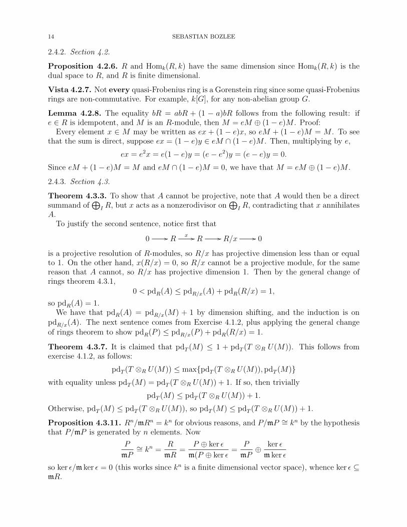
Lemma 4.2.8. The equality bR = abR + (1 − a)bR follows from the following result: ife ∈ R is idempotent, and M is an R-module, then M = eM ⊕ (1− e)M . Proof:
Every element x ∈ M may be written as ex + (1 − e)x, so eM + (1 − e)M = M . To seethat the sum is direct, suppose ex = (1− e)y ∈ eM ∩ (1− e)M . Then, multiplying by e,
ex = e2x = e(1− e)y = (e− e2)y = (e− e)y = 0.
Since eM + (1− e)M = M and eM ∩ (1− e)M = 0, we have that M = eM ⊕ (1− e)M .
2.4.3. Section 4.3.
Theorem 4.3.3. To show that A cannot be projective, note that A would then be a directsummand of
⊕I R, but x acts as a nonzerodivisor on
⊕I R, contradicting that x annihilates
A.To justify the second sentence, notice first that
0 // Rx // R // R/x // 0
is a projective resolution of R-modules, so R/x has projective dimension less than or equalto 1. On the other hand, x(R/x) = 0, so R/x cannot be a projective module, for the samereason that A cannot, so R/x has projective dimension 1. Then by the general change ofrings theorem 4.3.1,
0 < pdR(A) ≤ pdR/x(A) + pdR(R/x) = 1,
so pdR(A) = 1.We have that pdR(A) = pdR/x(M) + 1 by dimension shifting, and the induction is on
pdR/x(A). The next sentence comes from Exercise 4.1.2, plus applying the general changeof rings theorem to show pdR(P ) ≤ pdR/x(P ) + pdR(R/x) = 1.
Theorem 4.3.7. It is claimed that pdT (M) ≤ 1 + pdT (T ⊗R U(M)). This follows fromexercise 4.1.2, as follows:
pdT (T ⊗R U(M)) ≤ max{pdT (T ⊗R U(M)), pdT (M)}with equality unless pdT (M) = pdT (T ⊗R U(M)) + 1. If so, then trivially
Proposition 4.3.11. Rn/mRn = kn for obvious reasons, and P/mP ∼= kn by the hypothesisthat P/mP is generated by n elements. Now
P
mP∼= kn =
R
mR=
P ⊕ ker ε
m(P ⊕ ker ε=
P
mP⊕ ker ε
m ker ε
so ker ε/m ker ε = 0 (this works since kn is a finite dimensional vector space), whence ker ε ⊆mR.
SOLUTIONS AND ELABORATIONS 15
2.4.4. Section 4.4.
Proposition 4.4.5. The Krull intersection theorem (see [2, Corollary 5.4]) tells us that∩xnR = 0. This is useful since 0 is a prime ideal if and only if R is a domain.
There are finitely many prime ideals of R by a theorem of Noether (see [2, Exercise 1.2]).We include a statement and a proof since I should do the exercise anyway:
If R is Noetherian, and I ⊆ R is an ideal then among the primes of R containing I, thereare only finitely many that are minimal with respect to inclusion.
Write P (I) for the set of minimal primes containing an ideal I of R. Select an ideal Imaximal among those so that |P (I)| = ∞. I is not prime, since if it were, we would haveP (I) = {I}. Therefore there exist f, g ∈ R so that f, g 6∈ I but fg ∈ I.
Consider a prime p ∈ P (I). Since fg ∈ I ⊆ p, either f ∈ p so (I, f) ⊆ p or elseg ∈ p so (I, g) ⊆ p. Since p was a minimal prime containing I, p is also a minimal primecontaining (I, f) or (I, g). Then P (I) ⊆ P ((I, f)) ∪ P ((I, g)), so either |P ((I, f))| = ∞ or|P ((I, g))| =∞, contradicting the maximality of I. The result follows.
The implication that m ⊆ Pi for some i is from “prime avoidance;” see [2, Lemma 3.3].Since m is maximal, we actually have that m = Pi, and since we have assumed that mcontains no prime ideals, this shows that there are no proper inclusions of prime ideals. Itfollows R has dimension 0.
Standard Facts 4.4.6. An associated prime ideal of R is a prime ideal of the formAnnR(M) for a prime R-module M . A prime R-module M is one so that AnnR(M) =AnnR(N) for any nonzero submodule N of M .
Corollary 4.4.12. The inequality sup{pd(R/I)} ≤ fd(R/m) comes from the previousproposition. Each module R/I is finitely generated (actually generated by one element)so the lemma tells us that pd(R/I) is the maximum integer d so that TorRd (R/I, k) 6= 0.Thus each pd(R/I) ≤ fd(k) = fd(R/m), giving the inequality.
2.4.5. Section 4.5.
2.5. Chapter 5.
2.6. Chapter 6.
2.7. Chapter 7.
2.8. Chapter 8.
2.8.1. Section 8.1. Although there are upper and lower indices used throughout this section,it does not appear that there is a convention for which go with simplicial objects and whichgo with cosimplicial objects. This appears to agree with other sources.
Lemma 8.1.2. 0 ≤ is ≤ · · · ≤ i1 ≤ m should be replaced by 0 ≤ is < · · · < i1 ≤ m in thestatement of the lemma.
To do: explain why the factorization is equal to αThis expression for α is unique since a different factorization into face maps and degenera-
cies would imply that different elements in the image are skipped or that different elementsin the domain are mapped to the same place.
16 SEBASTIAN BOZLEE
Example 8.1.8. The words “combinational” and “combinatorial” are used interchangeablyhere and later. According to the errata, the word “combinatorial” was intended, so we willuse the name combinatorial in these notes.
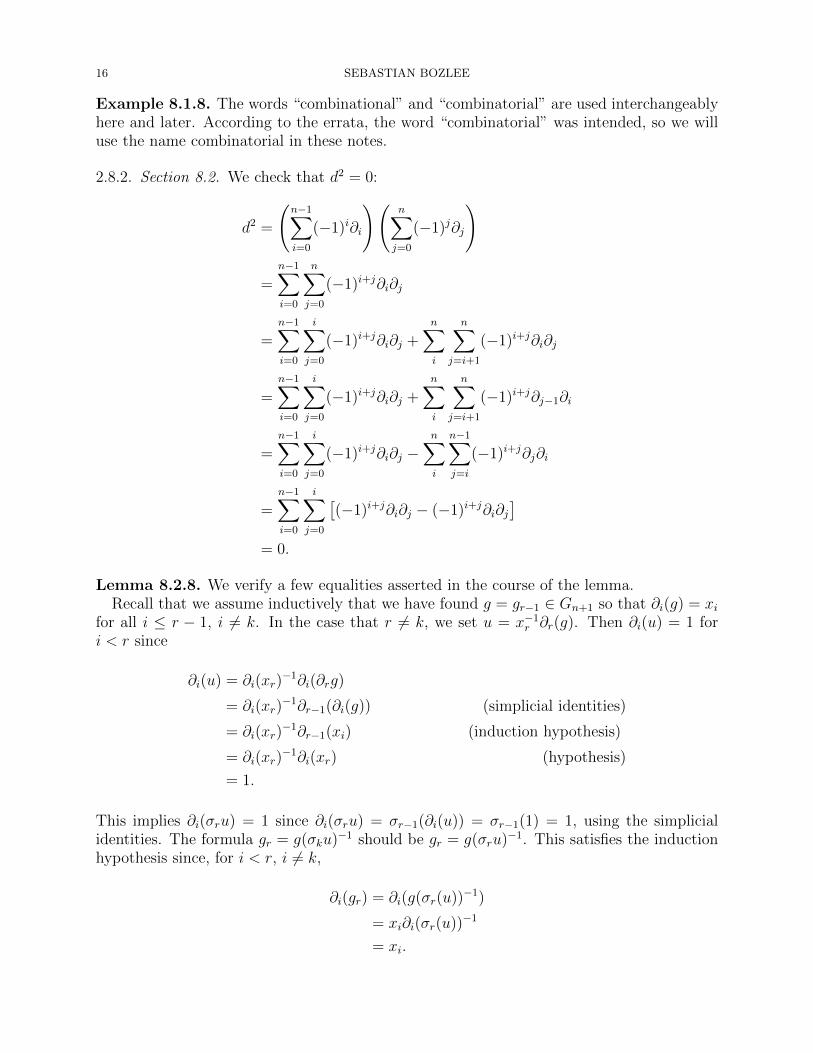
2.8.2. Section 8.2. We check that d2 = 0:
d2 =
(n−1∑i=0
(−1)i∂i
)(n∑j=0
(−1)j∂j
)
=n−1∑i=0
n∑j=0
(−1)i+j∂i∂j
=n−1∑i=0
i∑j=0
(−1)i+j∂i∂j +n∑i
n∑j=i+1
(−1)i+j∂i∂j
=n−1∑i=0
i∑j=0
(−1)i+j∂i∂j +n∑i
n∑j=i+1
(−1)i+j∂j−1∂i
=n−1∑i=0
i∑j=0
(−1)i+j∂i∂j −n∑i
n−1∑j=i
(−1)i+j∂j∂i
=n−1∑i=0
i∑j=0
[(−1)i+j∂i∂j − (−1)i+j∂i∂j
]= 0.
Lemma 8.2.8. We verify a few equalities asserted in the course of the lemma.Recall that we assume inductively that we have found g = gr−1 ∈ Gn+1 so that ∂i(g) = xi
for all i ≤ r − 1, i 6= k. In the case that r 6= k, we set u = x−1r ∂r(g). Then ∂i(u) = 1 for
i < r since
∂i(u) = ∂i(xr)−1∂i(∂rg)
= ∂i(xr)−1∂r−1(∂i(g)) (simplicial identities)
= ∂i(xr)−1∂r−1(xi) (induction hypothesis)
= ∂i(xr)−1∂i(xr) (hypothesis)
= 1.
This implies ∂i(σru) = 1 since ∂i(σru) = σr−1(∂i(u)) = σr−1(1) = 1, using the simplicialidentities. The formula gr = g(σku)−1 should be gr = g(σru)−1. This satisfies the inductionhypothesis since, for i < r, i 6= k,
∂i(gr) = ∂i(g(σr(u))−1)
= xi∂i(σr(u))−1
= xi.
SOLUTIONS AND ELABORATIONS 17
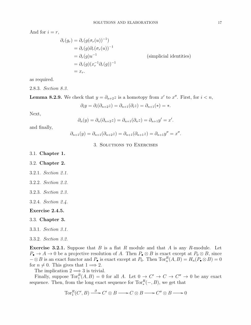
And for i = r,
∂r(gr) = ∂r(g(σr(u))−1)
= ∂r(g)∂r(σr(u))−1
= ∂r(g)u−1 (simplicial identities)
= ∂r(g)(x−1r ∂r(g))−1
= xr.
as required.
2.8.3. Section 8.3.
Lemma 8.2.9. We check that y = ∂n+2z is a homotopy from x′ to x′′. First, for i < n,
Exercise 3.2.1. Suppose that B is a flat R module and that A is any R-module. LetP• → A→ 0 be a projective resolution of A. Then P• ⊗ B is exact except at P0 ⊗ B, since−⊗B is an exact functor and P• is exact except at P0. Then TorRn (A,B) = Hn(P•⊗B) = 0for n 6= 0. This gives that 1 =⇒ 2.
The implication 2 =⇒ 3 is trivial.Finally, suppose TorR1 (A,B) = 0 for all A. Let 0 → C ′ → C → C ′′ → 0 be any exact
sequence. Then, from the long exact sequence for TorR∗ (−, B), we get that
TorR1 (C ′, B)∂ // C ′ ⊗B // C ⊗B // C ′′ ⊗B // 0
18 SEBASTIAN BOZLEE
is exact. By hypothesis, TorR1 (C ′, B) = 0, so in fact
0 // C ′ ⊗B // C ⊗B // C ′′ ⊗B // 0
is exact. Since 0 → C ′ → C → C ′′ → 0 was arbitrary, this shows − ⊗ B is exact, so B isflat. This gives the implication 3 =⇒ 1.
Exercise 3.2.2. Suppose that 0 → A → B → C → 0 is an exact sequence of R-modulesand A and C are flat R-modules. We take the long exact sequence associated to TorR∗ (−, D)for an R-module D and obtain that
is exact. Since A and C are flat, TorR1 (A,D) = 0 and TorR1 (C,D) = 0. By exactness,TorR1 (B,D) = 0. Since D was arbitrary, B is flat, by the implication 3 =⇒ 1 in thepreceding exercise.
Exercise 3.2.3. As hinted, we use the projective resolution of k given by
0 // R[−yx ]
// R2[x y ]
// R // k → 0.
From the projective resolution, we deduce that k is intended to be an R module by havingx and y act on k trivially, and the constants act by the usual multiplication.
Now we compute TorR2 (k, k) as the cohomology at the second location of the complex
0 // R⊗ k[−yx ]⊗1
// R2 ⊗ k[x y ]⊗1
// R⊗ k // 0,
which may be rewritten
0 // k[−yx ]
// k2[x y ]
// k // 0.
This is the same as the kernel of the map [ −yx ]. But x and y both act as zero on k, so thiskernel is k. Thus TorR2 (k, k) = k.
Next, we establish the isomorphism TorR1 (I, k) ∼= TorR2 (k, k) by a long exact sequenceargument. Consider the short exact sequence
0 // I // R // k // 0.
A portion of the associated long exact sequence under the homological δ-functor TorR∗ (−, k)is
Since R is projective, each of the modules on the ends are zero. By exactness, TorR1 (I, k) ∼=TorR2 (k, k). Combining this with the previous paragraph TorR1 (I, k) = k, so I is not flat,despite being torsionfree.
Exercise 3.2.4. Let A → B → C be an exact sequence of R-modules. Then since Q/Z isan injective abelian group (since Q/Z is divisible: see Corollary 2.3.2), HomAb(−,Q/Z) isan exact functor from Ab to Ab. Since the forgetful functor F from R-mod to Ab is alsoexact, the composition HomAb(F (−),Q/Z) is an exact functor. The image of A→ B → Cunder this composition is A∗ → B∗ → C∗, so A∗ → B∗ → C∗ is exact.
Conversely, suppose To do
SOLUTIONS AND ELABORATIONS 19
3.3.3. Section 3.3.
Exercise 3.3.1. We use the long exact sequence of the functor Ext∗Z(−,Z) associated to theshort exact sequence
0 // Z // Z[1p] // Zp∞ // 0,
then hijack the calculation given in Example 3.3.3. Since Hom is contravariant in its firstinput, Ext is a contravariant cohomological δ-functor in its first input, which means thatthe order of the parts of the short exact sequence is reversed in the long exact sequence andindices on Ext are increasing. The relevant portion of the long exact sequence is
Hom(Z[1p],Z) // Hom(Z,Z) // Ext1
Z(Zp∞ ,Z) // Ext1Z(Z[1
p],Z) // Ext1
Z(Z,Z).
First, we show Hom(Z[1p],Z) = 0. Suppose 1 7→ a under a homomorphism ϕ : Z[1
p] → Z.
Then ϕ( 1pn
) 7→ apn
for all n; that is, 1pn
is mapped to an element of Z whose pnth multiple is
a. This is impossible unless a = 0, so Hom(Z[1p],Z) = 0.
Next, Hom(Z,Z) ∼= Z. By the universal property of free abelian groups, any grouphomomorphism Z→ Z is determined by the image of 1, and conversely, the image of 1 maybe chosen freely. Then if ϕa : Z → Z denotes the group homomorphism such that 1 7→ a,the map a 7→ ϕa is clearly a group isomorphism Z→ Hom(Z,Z).
Next, Ext1Z(Zp∞ ,Z) = Zp by Exercise 3.3.3.
Next, Ext1Z(Z,Z) = 0, since Z is projective.
Our exact sequence now looks like
0 // Z // Zp // Ext1(Z[1p],Z) // 0
So Ext1(Z[1p],Z) is the quotient of Zp by some subgroup isomorphic to Z. I have not checked
that this subgroup is the is usual subgroup identified with Z.The next isomorphism we were given to prove, Zp/Z ∼= Zp∞ , is false. This can be checked
by noting that Zp/Z has an element of order m where m is relatively prime to p (namely[ 1m
]) while Zp∞ does not. The error is acknowledged in the errata online.
Exercise 3.3.2. Let R = Z/m and B = Z/p with p | m, so that B is an R-module. Wemust show that
0 // Z/p i // Z/mp // Z/m
m/p// Z/m
p // Z/mm/p
// · · ·
is an infinite periodic injective resolution of B. The first arrow is the inclusion map, pdenotes multiplication by p (mod m), and m/p denotes multiplication by m/p (mod m).Multiplication by p in Z/m vanishes precisely on Z/p = (m/p)Z/m and multiplication bym/p in Z/m vanishes precisely on pZ/m, so this is an exact sequence. Each of the modulesZ/m are injective by Exercise 2.3.1, so this is actually an injective resolution of B.
To compute Ext∗Z/m(A,Z/p) we take the cohomology of the image of the injective resolutionabove under the functor HomZ/m(A,−), namely
0 // A∗p∗ // A∗
(m/p)∗// A∗
p∗ // A∗(m/p)∗
// · · ·
20 SEBASTIAN BOZLEE
where A∗ is shorthand for HomZ/m(A,Z/m) as suggested in the problem statement. Thenwe get that
ExtnZ/m(A,Z/m) =
A∗ if n = 0
ker(m/p)∗/im p∗ if n > 0 is odd
ker p∗/im (m/p)∗ if n > 0 is even
Consider the case thatA = Z/p and p2 | m. Then we may identifyA∗ = HomZ/m(Z/p,Z/m)with (m/p)Z/m ∼= Z/p via the isomorphism ϕ 7→ ϕ(1). This is injective since each homo-morphism is determined by the image of 1 and surjective since each homomorphism musttake 1 to (p/m)Z/m ⊆ Z/m by order considerations. Now note that p and m/p both act aszero on Z/p since both are divisible by p. It follows that each kernel in the chain complex isZ/p and each image is 0. Taking quotients,
ExtnZ/m(Z/p,Z/m) = Z/p,for all n ≥ 0.
3.3.4. Section 3.4.
Exercise 3.4.1. Suppose
(8) 0 // Z/p // X // Z/p // 0
is an extension of Z/p by Z/p in Ab. We know from finite group theory that any extensionof a group A by a group B has order |A||B|. In this case, the group X must have order p2.By the fundamental theorem of abelian groups, X ∼= Z/p⊕Z/p or X ∼= Z/p2. We will showthat in each case the extension above is equivalent to one of the given extensions. Then wewill show that each of the given extensions are distinct.
Suppose first that X ∼= Z/p ⊕ Z/p. Let (a, b) ∈ Z/p ⊕ Z/p be the image of 1 under themap Z/p→ Z/p⊕ Z/p and let (c, d) be a preimage of 1 under the map Z/p⊕ Z/p→ Z/p.Then (c, d) and (a, b) form a basis of Z/p⊕ Z/p, viewing Z/p⊕ Z/p as a Z/p vector space,since (c, d) 6∈ ker{Z/p ⊕ Z/p → Z/p} = Span {(a, b)} and Z/p ⊕ Z/p has dimension two.Let ϕ : Z/p⊕ Z/p→ Z/p⊕ Z/p be the Z/p-linear (hence Z-linear) map that takes (a, b) to(1, 0) and (c, d) to (0, 1). This is an isomophism since we take a basis to a basis. Then thefollowing diagram commutes, where the first row is the extension (8) and the second row isthe usual split extension:
0 // Z/p // Z/p⊕ Z/p //
ϕ
��
Z/p // 0
0 // Z/p i // Z/p⊕ Z/p π // Z/p // 0
Next suppose that X ∼= Z/p2. The image of Z/p → Z/p2 must be pZ/p2, as it is theunique subgroup of Z/p2 of order p. Then 1 is mapped by Z/p → Z/p2 to some element ofthe form ap. Let b be the image of 1 under the map Z/p2 → Z/p. Let ϕ : Z/p2 → Z/p2 bethe map taking 1 to a−1. This is an isomorphism since a is relatively prime to p. Then thediagram
0 // Z/p // Z/p2 //
ϕ
��
Z/p // 0
0 // Z/pp // Z/p2 ab // Z/p // 0
SOLUTIONS AND ELABORATIONS 21
commutes, where the top row is extension (8) and the bottom row is one of the givenextensions, where i = ab.
Now we have to show that the given extensions are distinct. Let
ξi : 0 // Z/pp // Z/p2 i // Z/p // 0.
Since Z/p⊗ Z/p 6∼= Z/p2, we really only have to show that the ξi are distinct. Suppose
0 // Z/pp // Z/p2 i //
ϕ
��
Z/p // 0
0 // Z/pp // Z/p2 j // Z/p // 0
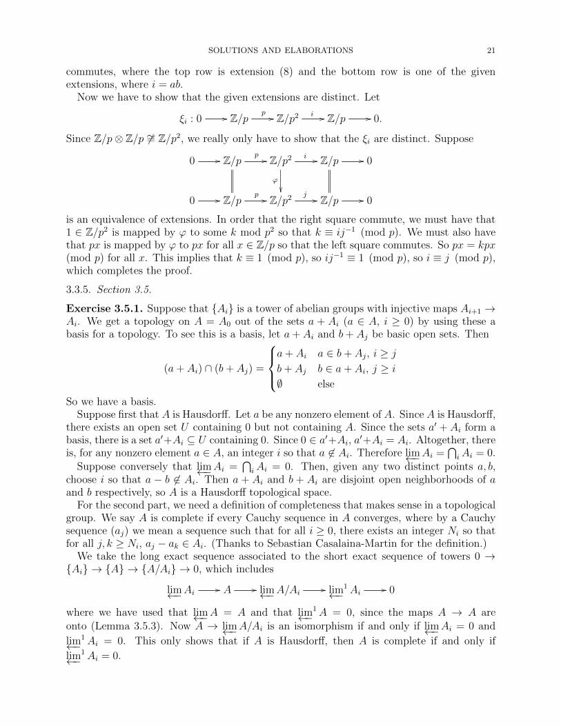
is an equivalence of extensions. In order that the right square commute, we must have that1 ∈ Z/p2 is mapped by ϕ to some k mod p2 so that k ≡ ij−1 (mod p). We must also havethat px is mapped by ϕ to px for all x ∈ Z/p so that the left square commutes. So px = kpx(mod p) for all x. This implies that k ≡ 1 (mod p), so ij−1 ≡ 1 (mod p), so i ≡ j (mod p),which completes the proof.
3.3.5. Section 3.5.
Exercise 3.5.1. Suppose that {Ai} is a tower of abelian groups with injective maps Ai+1 →Ai. We get a topology on A = A0 out of the sets a + Ai (a ∈ A, i ≥ 0) by using these abasis for a topology. To see this is a basis, let a+ Ai and b+ Aj be basic open sets. Then
(a+ Ai) ∩ (b+ Aj) =
a+ Ai a ∈ b+ Aj, i ≥ j
b+ Aj b ∈ a+ Ai, j ≥ i
∅ else
So we have a basis.Suppose first that A is Hausdorff. Let a be any nonzero element of A. Since A is Hausdorff,
there exists an open set U containing 0 but not containing A. Since the sets a′ + Ai form abasis, there is a set a′+Ai ⊆ U containing 0. Since 0 ∈ a′+Ai, a′+Ai = Ai. Altogether, thereis, for any nonzero element a ∈ A, an integer i so that a 6∈ Ai. Therefore lim←−Ai =
⋂iAi = 0.
Suppose conversely that lim←−Ai =⋂iAi = 0. Then, given any two distinct points a, b,
choose i so that a − b 6∈ Ai. Then a + Ai and b + Ai are disjoint open neighborhoods of aand b respectively, so A is a Hausdorff topological space.
For the second part, we need a definition of completeness that makes sense in a topologicalgroup. We say A is complete if every Cauchy sequence in A converges, where by a Cauchysequence (aj) we mean a sequence such that for all i ≥ 0, there exists an integer Ni so thatfor all j, k ≥ Ni, aj − ak ∈ Ai. (Thanks to Sebastian Casalaina-Martin for the definition.)
We take the long exact sequence associated to the short exact sequence of towers 0 →{Ai} → {A} → {A/Ai} → 0, which includes
lim←−Ai// A // lim←−A/Ai
// lim←−1Ai // 0
where we have used that lim←−A = A and that lim←−1A = 0, since the maps A → A are
onto (Lemma 3.5.3). Now A → lim←−A/Ai is an isomorphism if and only if lim←−Ai = 0 and
lim←−1Ai = 0. This only shows that if A is Hausdorff, then A is complete if and only if
lim←−1Ai = 0.
22 SEBASTIAN BOZLEE
To complete the proof, we show that if A is Hausdorff, A is complete if and only if theinduced map A → lim←−A/Ai is an isomorphism. (The problem statement is adjusted in theerrata.)
First, suppose (aj) is a Cauchy sequence. For each i, let Ni be as in the definition ofCauchy sequence. Note that then for all i, j ≥ Ni, aj ≡ ai (mod Ai). Let ϕ((aj))i = aNi(mod Ai). Then ϕ((aj)) is an element of lim←−A/Ai. Now suppose that ϕ((aj)) = ϕ((bj)) fortwo Cauchy sequences (aj) and (bj). Then (aj) and (bj) are equivalent Cauchy sequences.Conversely, given (bj) ∈ lim←−A/Ai, we can find a Cauchy sequence (aj) so that ϕ((aj)) = (bj)by choosing each aj to be a lift of bj in A. This tells us that lim←−A/Ai is the completion of A;that is, it is the space of Cauchy sequences in A modulo equivalence of Cauchy sequences.
Now the induced map lim←−A→ lim←−A/Ai is defined by (a) 7→ ([a]). That is, its image is thespace of equivalence classes of Cauchy sequences that are equivalent to a constant sequence.This map is an isomorphism if and only if all Cauchy sequences converge if and only if A iscomplete.
Exercise 3.5.2. Suppose that {Ai} is a tower of finite abelian groups. Denote by ϕj,k themap Aj → Ak. Then for any k, the sequence of subgroups ϕj,k(Aj) is decreasing in j (i.e.ϕj+1,k(Aj+1) ⊆ ϕj,k(Aj)). Since the collection of subgroups is finite, ϕj,k(Aj) must eventuallybe constant; that is, {Ai} must satisfy the Mittag-Leffler condition. By Proposition 3.5.7,lim←−
1Ai = 0.Similarly, suppose that {Ai} is a tower of finite-dimensional vector spaces. Then for
any k, the sequence ϕj,k(Aj) is decreasing in j. In particular, the dimension of ϕj,k(Aj)is decreasing. Since the dimension is strictly positive, this implies that the dimension ofϕj,k(Aj) is eventually constant. Then since ϕj,k(Aj) is also decreasing, this implies thatϕj,k(Aj) is also eventually constant. Therefore {Ai} satisfies the Mittag-Leffler condition, soby the proposition lim←−
1Ai = 0.
Exercise 3.5.5. Suppose
Ax
ϕ
��Ay
ψ// Az
is an element of AI . So that we can deal with elements, I will let A = R-mod.The only nonzero terms of the associated cochain complex are C0 and C1, so the only
differential we have to worry about is the differential d : C0 → C1. By definition, the objectC0 is Ax×Ay×Az, with the terms corresponding to the chains x, y, and z respectively, and theobject C1 is Az×Az with the first term of the product corresponding to the chain x < z andthe other term coresponding to the chain y < z. Following definitions again, d0 : C0 → C1
is defined by (a, b, c) 7→ (ϕ(a), ψ(b)) and d1 : C0 → C1 is defined by (a, b, c) 7→ (c, c). Allother dp are zero, so the differential d : C0 → C1 has the formula d0 − d1 which takes(a, b, c) 7→ (ϕ(a)− c, ψ(b)− c).
The kernel of d is then
{(a, b, c) ∈ C0 | ϕ(a) = ϕ(b) = c}
which is isomorphic to
{(a, b) ∈ Ax × Ay | ϕ(a) = ϕ(b)},
SOLUTIONS AND ELABORATIONS 23
the traditional concrete form given to the pullback of Ax and Ay over Az. This gives thatH0(C∗) is the pullback, as desired.
Next, since d : C1 → C2 is zero, H1(C∗) is the cokernel of d : C0 → C1. Since ∆ = {(c, c) :c ∈ Az} = d(0×0×Az) is contained in im d, we may quotient out by it first. More explicitly,we have the diagram with exact rows
C0d //
i
��
C1//
j
��
H1(C∗) // 0
Ax × Ayd // Az // H1(C∗) // 0
where i : (a, b, c) 7→ (a, b), j : (c, c′) 7→ c− c′ and d : (a, b) 7→ (ϕ(a)− ψ(b)). This commutessince ker i = 0 × 0 × Az, ker j = ∆ = d(ker i), and ∆ ⊆ ker{C1 → H1(C∗). This makesH1(C∗) the cokernel of the difference map, as claimed.
3.4. Chapter 4.
3.4.1. Section 4.1.
Exercise 4.1.1.
Exercise 4.1.2. The proof is by taking long exact sequences. We’ll tackle the projectivedimension part, then claim that the other parts have analogous proofs.
Suppose that d > pd(A) and d > pd(B). Then for any R-module D,
Extd(C,D) // Extd(B,D) // Extd(A,D)
is exact, and Extd(C,D) = Extd(A,D) = 0, so Extd(B,D) = 0. By the pd Lemma, pd(B) ≤max{pd(A), pd(C)} as desired. For the other inequality, suppose first that ∞ > pd(C) >
pd(A) + 1. By the pd Lemma, there is some R-module D so that Extpd(C)(C,D) 6= 0. Thelong exact sequence associated to Ext∗(−, D) contains the sequence
By hypothesis, the terms on the ends are zero, so Extpd(C)(B,D) 6= 0, which proves pd(B) ≥pd(C) = max{pd(A), pd(C)}. Next, suppose pd(C) < pd(A) + 1 < ∞. There is an R-
module D so that Extpd(A)(A,D) 6= 0. This gives us the exact sequence
Extpd(A)(B,D) // Extpd(A)(A,D) // Extpd(A)+1(C,D)
By assumption, the term on the right vanishes, so by exactness, Extpd(A)(B,D) 6= 0. Thisproves pd(B) ≥ pd(A) = max{pd(A), pd(C)}, when both pd(A) and pd(C) are finite.
When pd(A) is infinite but pd(C) is not, the long exact sequence associated to Ext∗(−, D)for any D eventually becomes a sequence of isomorphisms of Extp(B,D) with Homp(A,D).By choosing Dp so that Homp(A,Dp) is nonzero for each p, we get that pd(B) = ∞, asdesired. The same argument works in the case that pd(A) is finite while pd(C) is infinite,which completes the proof.
When pd(A) = pd(C) = ∞ (in which case pd(C) = pd(A) + 1 could be interpreted astrue) we need not have equality, as is shown by the short exact sequence 0→ Z/p→ Z/p2 →Z/p→ 0 in the category of Z/p2 modules. Here pd(Z/p) =∞ (see Calculation 3.1.6) whilepd(Z/p2) = 0, since Z/p2 is projective.
24 SEBASTIAN BOZLEE
It’s interesting to see that the result cannot be strengthened to include pd(C) = pd(A)+1
even with finite projective dimensions, since 0 → Z p→ Z → Z/p → 0 is a counterexampleover Z-modules. More generally, for any non-projective C, we can find a short exact sequence0→M → F → C → 0 where F is free, so we have a counterexample for every non-projectiveobject C.
Parts 2 and 3 have exactly analogous proofs. For the second part, we take long exactsequences with respect to Ext∗(D,−) instead of Ext∗(−, D), and in the third part we takelong exact sequences with respect to Tor∗(−, D). The short exact sequence 0 → Z → Q →Q/Z → 0 is an example that shows the second part’s result cannot be strengthened toinclude the case that id(A) = id(C) + 1.
Exercise 4.1.3.
(1) First, choose a projective resolution Pi → Ai of minimal length for each i. Then⊕i Pi →
⊕iAi is a projective resolution of
⊕iAi. The length of
⊕Pi is the given
supremum, so
pd(⊕
Ai) ≤ sup{pd(Ai)}.To do: other inequality.
(2)(3) Choose a sequence of R-modules Ai such that pd(Ai) ≥ i for each i ∈ N. Then by
part 1, A =⊕
iAi is a module with infinite projective dimension.
3.4.2. Section 4.2.
Exercise 4.2.1. Z/m is Noetherian because it is finite. To show that Z/m is injective, weuse Baer’s criterion (2.3.1). Each ideal of Z/m is of the form (n). By order considerations,any map (n) → Z/m must take n 7→ k · n, and since (n) is cyclic this determines the map.This extends to the map Z/m→ Z/m determined by 1 7→ k. Therefore Z/m is also injectiveas a module over itself, and Z/m is quasi-Frobenius.
Exercise 4.2.5. Let a ∈ R. We want to show that there exists x ∈ R so that axa = a. Byhypothesis,
aR = eR
for some idempotent e. From this equality, there is some x ∈ R so that ax = e and somey ∈ R so that a = ey. Then axa = eey = ey = a, as desired.
Exercise 4.2.6.
3.4.3. Section 4.3.
Exercise 4.3.1. (Thanks to Jonathan Wise for the suggestion to use the local criterion forflatness.)
By the first change of rings theorem,
pdk[[x1,...,xn]](k) = 1 + pdk[[x1,...,xn−1]](k).
By induction and noting that pdk(k) = 0, pd(k) = n, so the global dimension of R is greaterthan or equal to n.
Since R is Noetherian, the flat and global dimensions of R coincide, so we now show thatthe flat dimension of M over R is less than n for all R-modules M . By the fd lemma, itis enough to show that Torn+1(M,N) = 0 for all R-modules N . Assume first that M is
SOLUTIONS AND ELABORATIONS 25
finitely generated. Then Torn+1(M,k) = 0, since fd(k) = pd(k) = n. By the local criterionfor flatness [2, Theorem 6.8], M is flat. If M is not finitely generated, write M as a colimitof its finitely generated submodules, lim−→MI . Then Torn+1(M,N) = lim−→Torn+1(MI , N) = 0.Therefore R has global dimension n.
Exercise 4.3.2. By the first change of rings theorem,
pdR(A/xA) = 1 + pdR/x(A/xA).
We need to relate pdR(A) with pdR(A/xA), so we consider the short exact sequence
0 // Ax // A // A/xA // 0
By Exercise 4.1.2, pdR(A) ≤ max{pdR(A), pdR(A/xA)}, with equality unless pdR(A/xA) =1 + pdR(A). If pdR(A) + 1 = pdR(A/xA), then pdR(A) = pdR/x(A/xA), and the theoremholds. Otherwise, we have that pdR(A) ≥ pdR(A/xA), so pdR(A) ≥ pdR/x(A/xA) + 1, andthe theorem holds.
Exercise 4.3.3.
3.4.4. Section 4.4.
Exercise 4.4.1. (Thanks again to Jonathan Wise for noting that the remark from the“Standard Facts” was applicable.)
Since R is a regular local ring, dimk(m/m2) = dim(R) = d. By the fourth isomorphism
theorem for rings, R/(x1, . . . , xi)R is local with maximal ideal m/(x1, . . . , xi)R. Now
(m/(x1, . . . , xi))2 = m2/(x1, . . . , xi)
so the quotient in question is(m
(x1, . . . , xi)
)/
(m2
(x1, . . . , xi)
)∼=
m
m2 + (x1, . . . , xi)∼=( m
m2
)/
((x1, . . . , xi)
m2
)which has dimension d− i.
It remains to check that the Krull dimension of R/(x1, . . . , xd)R is as claimed. By theremark in the “Standard Facts” following this exercise, if x is a nonzerodivisor on R, thenR/x has dimension dimR− 1. Inductively, R/(x1, . . . , xd) has dimension d− i as desired.
Exercise 4.4.2.
3.4.5. Section 4.5.
Exercise 4.5.1.
(1) We define the product of [a] ∈ ker dp/im dp+1 and [b] ∈ ker dq/im dq+1 to be theelement [ab] ∈ ker dp+q/im dp+q+1. To show this is well defined, suppose a = a′+d(α)for some α ∈ Kp+1 and b = b′ + d(β) for some β ∈ Kq+1. Now
ab− a′b′ = d(α)b+ ad(β) + d(α)d(β).
I claim the right side is equal to d(αb+ aβ + αd(β)):
where the second equality follows from the assumption that a, b ∈ ker d and d2 = 0.This shows that the products of different representatives differ by an element ofim dp+q+1, so the product is well defined.
Associativity, distributivity, and graded commutativity come directly from thecorresponding properties of K after reduction modulo the image of d.
(2) We will need to assume that R is commutative.To see d2 = 0, it suffices to check that this holds on basis vectors. Suppose
In the second equality, the first sum is over those summands where a smaller index wasremoved in the second application of d and the second sum is over those summandswhere a larger index was removed in the second application of d. The third equalityfollows by pairing summands containing the same basis vector.
We also need to check that the Leibnitz rule holds. For convenience, we will showfirst that the formula given for d of a standard basis vector is independent of the orderin which it is written as a wedge product of the ei. For this, it suffices to show thatswapping two adjacent elements changes the sign of the result. (This will also showthat if some ei is repeated, the formula for d correctly gives zero.) More concretely,we wish to show that if σ is the transposition (j, j + 1)
Next, the wedge product functions as a product which respects the grading andis graded-commutative. We have now shown that the Koszul complex K(x) is agraded-commutative DG-algebra.
The desired external product is defined by the bilinear map
(a(ei1 ∧ · · · ∧ eip), b(ej1 ∧ · · · ∧ ejq)) 7→ a⊗ b(ei1 ∧ · · · ∧ eip ∧ ej1 ∧ · · · ∧ ejq).The Koszul homology is a graded-commutative R-algebra by the part 1.
(3) We note that since each xi ∈ I acts as zero, each map in the Koszul complex is thezero map. It follows that the homology is isomorphic to the Koszul complex itself,Λ∗(An).
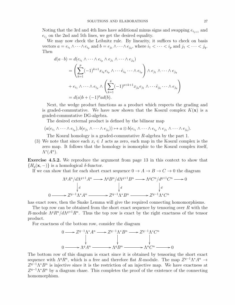
Exercise 4.5.2. We reproduce the argument from page 13 in this context to show that{Hq(x,−)} is a homological δ-functor.
If we can show that for each short exact sequence 0→ A→ B → C → 0 the diagram
ΛqAn/dΛq+1An //
d��
ΛqBn/dΛq+1Bn //
d��
ΛqCn/dq+1Cn //
d��
0
0 // Zq−1Λ∗An // Zq−1Λ∗Bn // Zq−1Λ∗Cn
has exact rows, then the Snake Lemma will give the required connecting homomorphisms.The top row can be obtained from the short exact sequence by tensoring over R with the
R-module ΛqRn/dΛq+1Rn. Thus the top row is exact by the right exactness of the tensorproduct.
For exactness of the bottom row, consider the diagram
0 // Zq−1Λ∗An //
��
Zq−1Λ∗Bn //
��
Zq−1Λ∗Cn
��0 // ΛqAn // ΛqBn // ΛnCn // 0
The bottom row of this diagram is exact since it is obtained by tensoring the short exactsequence with ΛqRn, which is a free and therefore flat R-module. The map Zq−1Λ∗An →Zq−1Λ∗Bn is injective since it is the restriction of an injective map. We have exactness atZq−1Λ∗Bn by a diagram chase. This completes the proof of the existence of the connectinghomomorphism.
28 SEBASTIAN BOZLEE
For naturality of the connecting homomorphism, we can repeat the argument of Proposi-tion 1.3.4, noting that Hq(x,−) is a functor, since it is the composition of the homology andΛ∗Rn ⊗− functors. This completes the proof that {Hq(x,−)} is a homological δ-functor.
To do: {Hq(x,−)}.
Exercise 4.5.3.
Exercise 4.5.4. By Exercise 1.4.3, it suffices to show that there is a chain contraction s ofthe identity map. Suppose without loss of generality that x1 is the unit. I claim that themaps {sq} defined by
So id = ds+ sd, as desired.The groups H∗(x, A) = H∗(x, A) = 0 are zero since split exact sequences are preserved by
additive functors, namely −⊗ A and Hom(−, A).
3.5. Chapter 5.
3.6. Chapter 6.
3.7. Chapter 7.
3.8. Chapter 8.
3.8.1. Section 8.1.
Exercise 8.1.1. Recall that εi : [n− 1]→ [n] and ηi : [n+ 1]→ [n] are defined by
εi(j) =
{j if j < i
j + 1 if j ≥ i
and
ηi(j) =
{j if j ≤ i
j − 1 if j > i
To get the idea of what’s going on, it helps to draw a picture of each simplicial identity forn = 4 or so. Of course, this won’t do for a proof, so now we plug and chug. Fix an integer
SOLUTIONS AND ELABORATIONS 29
n greater than or equal to zero, and assume i, j are integers so that 0 ≤ i < j ≤ n. Then
εj(εi(k)) =
{εj(k) if k < i
εj(k + 1) if k ≥ i
=
k if k < i and k < j
k + 1 if k < i and k ≥ j
k + 1 if i ≤ k and k + 1 < j
k + 2 if i ≤ k and k + 1 ≥ j
=
k if k < i
k + 1 if i ≤ k ≤ j
k + 2 if j < k
while
εi(εj−1(k)) =
{εi(k) if k < j − 1
εi(k + 1) if k ≥ j − 1
=
k if k < j − 1 and k < i
k + 1 if k < j − 1 and k ≥ i
k + 1 if k ≥ j − 1 and k + 1 < i
k + 2 if k ≥ j − 1 and k + 1 ≥ i
=
k if k < i
k + 1 if i ≤ k ≤ j
k + 2 if j < k
so εjεi = εiεj−1. Intutively, εiεj−1 inserts a space at the j − 1st spot then the ith spot of[n]. If we were to do this in the opposite order, we would have to take into account that thej − 1st element of [n] is moves one spot to the right after inserting a space at the ith spot,so εjεi = εiεj−1.
Next, with the same hypotheses,
ηj(ηi(k)) =
{ηj(k) if k ≤ i
ηj(k − 1) if k > i
=
k if k ≤ i and k ≤ j
k − 1 if k ≤ i and k > j
k − 1 if k > i and k − 1 ≤ j
k − 2 if k > i and k − 1 > j
=
k if k ≤ i
k − 1 if i < k ≤ j + 1
k − 2 if j + 1 < k
30 SEBASTIAN BOZLEE
while
ηi(ηj+1(k)) =
{ηi(k) if k ≤ j + 1
ηi(k − 1) if k > j + 1
=
k if k ≤ j + 1 and k ≤ i
k − 1 if k ≤ j + 1 and k > i
k − 1 if k > j + 1 and k − 1 ≤ i
k − 2 if k > j + 1 and k − 1 > i
=
k if k ≤ i
k − 1 if i < k ≤ j + 1
k − 2 if j + 1 < k
so ηjηi = ηiηj+1.If 0 ≤ i < j ≤ n, then
ηj(εi(k)) =
{ηj(k) if k < i
ηj(k + 1) if k ≥ i
=
k if k < i
k + 1 if i ≤ k and k + 1 ≤ j
k if k + 1 > j
=
k if k < i
k + 1 if i ≤ k < j
k if k ≥ j
while
εi(ηj−1(k)) =
{εi(k) if k ≤ j − 1
εi(k − 1) if k > j − 1
=
k if k < i
k − 1 if k ≤ j − 1 and k ≥ i
k if k > j − 1
=
k if k < i
k − 1 if i ≤ k < j
k if k ≥ j
so ηjεi = εiηj−1 in this case.If i = j or i+ 1 = j, then
ηj(εi(k)) =
{ηj(k) if k < i
ηj(k + 1) if k ≥ i
= k
SOLUTIONS AND ELABORATIONS 31
Finally, if j < i,
ηj(εi(k)) =
{ηj(k) if k < i
ηj(k + 1) if k ≥ i
=
k if k ≤ j
k − 1 if j < k < i
k if i ≤ k
while
εi−1(ηj(k)) =
{εi−1(k) if k ≤ j
εi−1(k − 1) if k > j
=
k if k ≤ j
k − 1 if k > j and k − 1 < i− 1
k if k − 1 ≥ i− 1
=
k if k ≤ j
k − 1 if j < k < i
k if i ≤ k
so ηjεi = εi−1ηj in this case, as required.
Exercise 8.1.2. Suppose that K is an ordered combinatorial simplicial complex consistingof subsets of V . Then given any subset W = {v0, . . . , vn} ∈ K, with v0 < v1 < · · · < vn,we get a corresponding element (v0, . . . , vn) ∈ SSn(K). This cannot be degenerate, as anydegenerate n-simplex has a repeated index, while this has none.
Conversely, if (v0, . . . , vn) ∈ SSn(K) is nondegenerate, then {v0, . . . , vn} is in K, by defi-nition. This establishes the one-to-one correspondence.
Exercise 8.1.3. Note that each (v0, . . . , vk) in SSk(K) may be interpreted as a morphismv : [k]→ [n] in ∆ defined by i 7→ vi. This is a one-to-one correspondence. Recall that givenα : [l] → [k], we have defined α∗(v0, . . . , vk) = (vα(0), . . . , vα(l)). The associated morphismtakes i 7→ vα(i), so α∗ acts by precomposition on associated morphisms. That is, SS(K) isisomorphic to the functor Hom∆(−, [n]), and we will regard them as interchangeable fromhere on out.
Now, to each k and α ∈ Hom∆([k], [n]), we have an associated continuous map α∗ : ∆k →∆n (from Example 8.1.5, although there it is written with a lower star). These induce,by the universal property of coproducts, a map ϕ :
∐k SS(K) × ∆k → ∆n defined by
(α, x) 7→ α∗(x). Going the other direction, we have the map ψ : ∆n →∐
k SS(K)×∆k thatincludes ∆n into the copy of ∆n corresponding to id[n]. Clearly, ϕ ◦ ψ = id∆n .
Next, I claim that (α, x) ∈ SSk(K)×∆k is equivalent (see 8.1.6) to (β, y) ∈ SSl(K)×∆l
if and only if ϕ(α, x) = ϕ(β, y). Suppose first that ϕ(α, x) = ϕ(β, y). Then α∗(x) = β∗(y),so
It is clear that ϕ(α, x) = ϕ(β, y) is an equivalence relation, so for the other implication itsuffices to show that if there is γ : [l] → [k] so that (α ◦ γ, x) = (β, γ∗(y)), then ϕ(α, x) =
Therefore ϕ respects the equivalence relation. The universal property of quotients thentells us that ϕ factors uniquely through the quotient map π :
∐k SSk(K)×∆k → |SS(K)|
as ϕ : |SS(K)| → ∆n. In fact, since points are equivalent if and only if their images underϕ agree, ϕ is a bijection. It remains to see that its inverse function is continuous. For this,we note that
id∆n = ψ ◦ ϕ = ψ ◦ π ◦ ϕ,so ψ ◦ π is its ϕ’s inverse, and ψ ◦ π is continuous. Altogether, |SS(K)| ∼= ∆n.
Exercise 8.1.4.
Exercise 8.1.5.
Exercise 8.1.6. Considering Lemma 8.1.2 in the case that α : [n] → [m] is injective, weget that every morphism in ∆s is a composition of face maps. Therefore a semi-simplicialobject K : ∆s → A is determined by its values on objects, Kn = K([n]), and its values onface maps, ∂i : Kn → Kn−1 = K(εi : [n − 1] → [n]), for i = 0, . . . , n. We know from thesimplicial identities that ∂i∂j = ∂j−1∂i when i < j.
On the other hand, given objects Kn and morphisms ∂i satisfying ∂i∂j = ∂j−1∂i for i < j,we get a semi-simplicial object since, the relations ∂i∂j = ∂j−1∂j determine all relationsamong the εi in ∆s. (To Do: This is a bit handwavey. Why is this a complete set ofrelations?)
3.8.2. Section 8.2.
Exercise 8.2.1. We did this in Exercise 8.1.3.
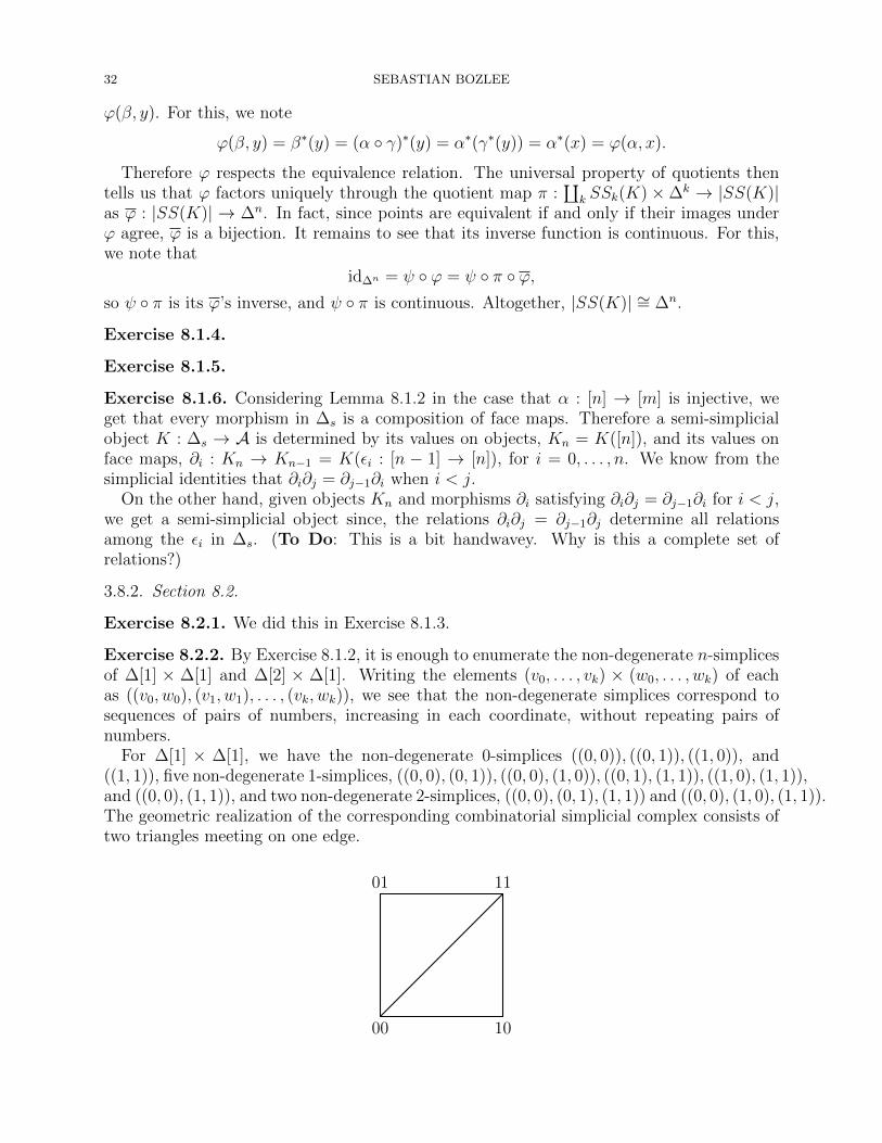
Exercise 8.2.2. By Exercise 8.1.2, it is enough to enumerate the non-degenerate n-simplicesof ∆[1] × ∆[1] and ∆[2] × ∆[1]. Writing the elements (v0, . . . , vk) × (w0, . . . , wk) of eachas ((v0, w0), (v1, w1), . . . , (vk, wk)), we see that the non-degenerate simplices correspond tosequences of pairs of numbers, increasing in each coordinate, without repeating pairs ofnumbers.
For ∆[1] × ∆[1], we have the non-degenerate 0-simplices ((0, 0)), ((0, 1)), ((1, 0)), and((1, 1)), five non-degenerate 1-simplices, ((0, 0), (0, 1)), ((0, 0), (1, 0)), ((0, 1), (1, 1)), ((1, 0), (1, 1)),and ((0, 0), (1, 1)), and two non-degenerate 2-simplices, ((0, 0), (0, 1), (1, 1)) and ((0, 0), (1, 0), (1, 1)).The geometric realization of the corresponding combinatorial simplicial complex consists oftwo triangles meeting on one edge.
00 10
01 11
SOLUTIONS AND ELABORATIONS 33
This is a square, just like |∆[1]| × |∆[1]|.For ∆[2] × ∆[1], the list of non-degenerate simplices gets unwieldy. We will just draw a
picture:
00
20
10
01
21
11
This is a triangular prism made up of three tetrahedrons, namely one with vertices 00, 01, 11, 21,another with vertices 00, 10, 11, 21, and finally one with vertices 00, 10, 20, 21. |∆[2]|× |∆[1]|is also a triangular prism, so |∆[2]×∆[1]| = |∆[2]| × |∆[1]|, as desired.
Exercise 8.2.3. Let n > 0. Consider x0 = (0, 1), x1 = (1, 1) in ∆[n]1. We have that∂0x1 = 1 = ∂0x0. In order that y ∈ ∆[n]2 satisfies ∂0y = x0 and ∂1y = x1, we would needy = (1, 0, 1). But this is not an increasing sequence, so ∆[n] is not fibrant.
To Do: Prove that a non-constant fibrant simplicial set must have non-degenerate n-cellsfor all n.
Exercise 8.2.4.
Exercise 8.2.5.
3.8.3. Section 8.3.
Exercise 8.2.6. Take G0 to act on G by g · h = σn0 (g)h for g ∈ G0, h ∈ Gn.
4. Additional Math
4.1. Short Exact Sequences.([3, p.132] and [1] provided the necessary hints to complete this section.)
Definition 1. A split exact sequence in an abelian category A is a sequence
0 // A′f // A
g // A′′ // 0
such that there exist maps ϕ : A′′ → A and ψ : A→ A′ so that
(1) g ◦ ϕ = idA′′ ,(2) ψ ◦ f = idA′ ,(3) g ◦ f = 0,(4) ψ ◦ ϕ = 0,(5) f ◦ ψ + ϕ ◦ g = idA.
(I don’t think anyone else defines a split exact sequence this way.)The next proposition shows that a split exact sequence can be thought of as one which
is “exact when read forwards as well as backwards,” or as a consequence, as a sequence inwhich both A′ and A′′ are subobjects as well as quotient objects of A.
34 SEBASTIAN BOZLEE
Proposition 2. If a sequence of R-modules
0 // A′f // A
g // A′′ // 0
is split exact, and we fix associated maps ϕ and ψ, then both 0 → A′f→ A
g→ A′′ → 0 and
0→ A′′ϕ→ A
ψ→ A′ → 0 are exact.
Proof. The map g is an epimorphism since g ◦ϕ = idA′′ , so the first sequence is exact at A′′.Similarly, f is a monomorphism since ψ ◦ f = idA′ , so the first sequence is exact at A′.
Next, ker g ⊇ im f , since g ◦ f = 0. For the other inclusion, let x ∈ ker g. Then
x = (f ◦ ψ + ϕ ◦ g)(x)
= f(ψ(x)) + ϕ(0) = f(ψ(x)).
so x ∈ im f . This proves the first sequence is exact at A.The second sequence is exact by a symmetric argument, since the definition is symmetric
under the exchange of g with ψ and f with ϕ. �
Other definitions of split exact sequences are equivalent to the one we have given by thefollowing proposition:
Proposition 3. Let 0→ A′f→ A
g→ A′′ → 0 be a short exact sequence of R-modules. Thefollowing are equivalent:
(1) 0→ A′f→ A
g→ A′′ → 0 is a split exact sequence.(2) There exists a map ϕ : A′′ → A so that g ◦ ϕ = idA′′ .(3) There exists a map ψ : A→ A′ so that ψ ◦ f = idA′ .(4) There exists an isomorphism τ : A → A′ ⊕ A′′ so that τ ◦ f is the usual inclusion
a′ 7→ (a′, 0) and g ◦ τ−1 is the usual projection (a′, a′′) 7→ a′′.
Proof. The implications (1) =⇒ (2) and (1) =⇒ (3) are trivial. We shall show (3) =⇒ (4),(4) =⇒ (1), and leave (2) =⇒ (4) as an adjustment of the proof that (3) =⇒ (4).
((3) =⇒ (4)) Suppose that ψ : A′′ → A is a map so that ψ ◦ f = idA′ . Note that for anyx ∈ A, we have that x− f(ψ(x)) ∈ kerψ, since
Thus, any x ∈ A can be written as a sum x = f(ψ(x)) + (x − f(ψ(x))). This impliesA = im f + kerψ. Suppose x ∈ im f and x ∈ kerψ. Then x = f(y) for some y in A′. Itfollows
x = f(y) = f(ψ(f(y))) = f(ψ(x)) = 0,
so in fact A = im f ⊕ kerψ.Let τ : A = im f ⊕ kerψ → A′⊕A′′ be defined by f(y) +w 7→ (y, g(w)), where w ∈ kerϕ.
We must show τ is an isomorphism. For injectivity suppose x = f(y) + w ∈ A and x′ =f(y′) + w′ ∈ A are elements of A so that τ(x) = τ(x′). Since f is an injection, y = y′. Byexactness, w − w′ ∈ im f , so w − w′ = 0. For surjectivity, let (a′, a′′) ∈ A′ ⊕ A′′. Then forany lift w ∈ A so that g(w) = a′′, f(a′) + (w − f(ψ(w))) is a preimage of (a′, a′′).
Clearly, τ ◦ f is the usual inclusion. Next, (g ◦ τ−1)(a′, a′′) = g(f(a′) + (w − f(ψ(w)))) =g(w) = a′′ is the usual projection, where w is any preimage of a′′ under g.
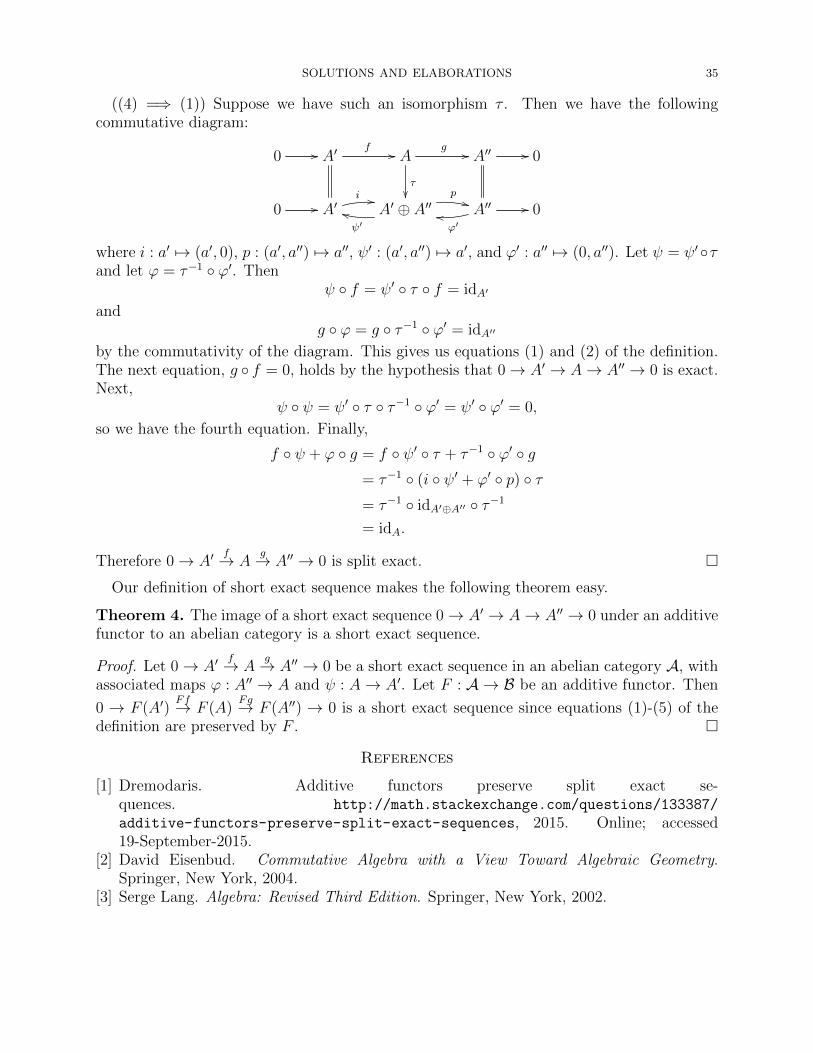
SOLUTIONS AND ELABORATIONS 35
((4) =⇒ (1)) Suppose we have such an isomorphism τ . Then we have the followingcommutative diagram:
0 // A′f // A
g //
τ��
A′′ // 0
0 // A′i ..
A′ ⊕ A′′p++
ψ′jj A′′ //
ϕ′nn 0
where i : a′ 7→ (a′, 0), p : (a′, a′′) 7→ a′′, ψ′ : (a′, a′′) 7→ a′, and ϕ′ : a′′ 7→ (0, a′′). Let ψ = ψ′◦τand let ϕ = τ−1 ◦ ϕ′. Then
ψ ◦ f = ψ′ ◦ τ ◦ f = idA′
andg ◦ ϕ = g ◦ τ−1 ◦ ϕ′ = idA′′
by the commutativity of the diagram. This gives us equations (1) and (2) of the definition.The next equation, g ◦ f = 0, holds by the hypothesis that 0→ A′ → A→ A′′ → 0 is exact.Next,
ψ ◦ ψ = ψ′ ◦ τ ◦ τ−1 ◦ ϕ′ = ψ′ ◦ ϕ′ = 0,
so we have the fourth equation. Finally,
f ◦ ψ + ϕ ◦ g = f ◦ ψ′ ◦ τ + τ−1 ◦ ϕ′ ◦ g= τ−1 ◦ (i ◦ ψ′ + ϕ′ ◦ p) ◦ τ= τ−1 ◦ idA′⊕A′′ ◦ τ−1
= idA.
Therefore 0→ A′f→ A
g→ A′′ → 0 is split exact. �
Our definition of short exact sequence makes the following theorem easy.
Theorem 4. The image of a short exact sequence 0→ A′ → A→ A′′ → 0 under an additivefunctor to an abelian category is a short exact sequence.
Proof. Let 0→ A′f→ A
g→ A′′ → 0 be a short exact sequence in an abelian category A, withassociated maps ϕ : A′′ → A and ψ : A→ A′. Let F : A → B be an additive functor. Then
0 → F (A′)Ff→ F (A)
Fg→ F (A′′) → 0 is a short exact sequence since equations (1)-(5) of thedefinition are preserved by F . �