202
An Introduction to Impact Dynamics An Introduction to Impact Dynamics Bernard Brogliato, INRIA Grenoble-Rhˆone-Alpes, France June 2010, Aussois 1
An Introduction to Impact Dynamics
An Introduction to Impact Dynamics
Bernard Brogliato, INRIA Grenoble-Rhone-Alpes, France
June 2010, Aussois
1

An Introduction to Impact Dynamics
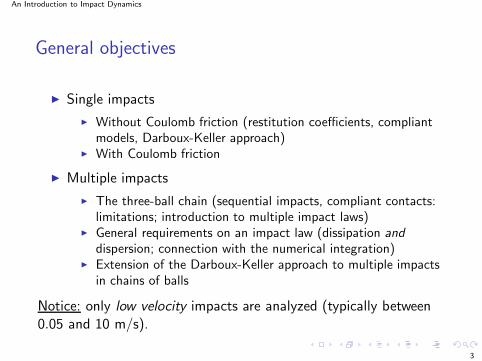
General objectives
Objective of these lectures: give an overview of various impactmodeling approaches with a focus on multiple impacts.
2
An Introduction to Impact Dynamics
General objectives
Single impacts
Without Coulomb friction (restitution coefficients, compliantmodels, Darboux-Keller approach)
With Coulomb friction
Multiple impacts
The three-ball chain (sequential impacts, compliant contacts:limitations; introduction to multiple impact laws)
General requirements on an impact law (dissipation anddispersion; connection with the numerical integration)
Extension of the Darboux-Keller approach to multiple impactsin chains of balls
Notice: only low velocity impacts are analyzed (typically between0.05 and 10 m/s).
3
An Introduction to Impact Dynamics
Some (pessimistic) philosophy
Quoted from [Chatterjee and Ruina, JAM 1998]:
There is no reason to believe that, in general, an accuratecontinuum model can be well approximated by treating the bodyas rigid everywhere except in a localized quasi-static regiondescribable by ordinary differential equations (as demanded byincremental laws).
4

An Introduction to Impact Dynamics
Some (pessimistic) philosophy, continued
Finally, there is no reason to expect that the outcome of detailedmodeling or exhaustive experimentation has a tractablesummarizing description with standard functions or even lookuptables that apply equally well to a wide variety of bodies and theircollisions (as is demanded by algebraic collision laws).
Any generally applicable collision law, whether coming fromdetailed continuum modeling, approximating ordinary differentialequations, or summarizing functions, will be highly approximateunless applied to a narrow range of collisional situations.
5
An Introduction to Impact Dynamics
Some (pessimistic) philosophy, continued
Fundamentally, the source of the difficulty is that one wants torepresent a complex dynamical process (deformable bodies thatcollide: =⇒ PDEs of continuum mechanics) by a “law” or “rule”of the form:
V + = Function of (V−, parameters, configuration)
Is it reasonable to assume that a finite number of parameters(sometimes very small number) can well approximate bodiesdeformation ?
6
An Introduction to Impact Dynamics
Fortunately enough, after their pessimistic introduction, theauthors of the same paper propose a new impact law...
7

An Introduction to Impact Dynamics
Frictionless single impacts between two bodies
Single impacts
An impact is said single when two systems collide at one point.Here we consider two bodies which are locally convex around thecontact point.
If more than one contact closes at the same time we shall speak ofmultiple impacts.
8
An Introduction to Impact Dynamics
Frictionless single impacts between two bodies
Single impacts
We are going to review some collision mappings:
q+ = F(q−, q, parameters)
Which are the desirable properties for an impact mapping?
(a) Provide a unique solution for all data (b) Be numerically tractable (c) Possess mechanically sound parameters (like restitution
coefficients) (d) Be able to span the whole subspace of admssible
post-impact velocities (e) Be able to correctly predict impact outcomes for various
types of bodies (shapes, material) so that it may be validatedthrough experiments.
Meeting all of these requirements is not an easy task, even forsingle collisions. 9

An Introduction to Impact Dynamics
Frictionless single impacts between two bodies
Single impacts
Classes of impact dynamics modeling:
(1) Rigid bodies: (a) Purely algebraic (b) Quasi-static (Darboux-Keller, or Routh in 2D)
(2) Deformable bodies:
(a) Compliant model (elastic, visco-elastic, elasto-plastic;linear or nonlinear)
(b) FEM analysis
Models (2) may feed models (1) with analytical expressions forrestitution coefficients.
10
An Introduction to Impact Dynamics
Frictionless single impacts between two bodies
Rigid body model (algebraic impact dynamics)
Single impacts
Assuming that the impact is instantaneous, then it is an easymatter to deduce that the contact force is impulsive (a Diracmeasure) and that the impact dynamics is an algebraic relationbetween velocties and impulses (the impulse being the Diracmeasure magnitude). For two bodies colling at a single point thisgives a relation of the type :
MAi
Ω+i − Ω−
i
V +Ai
− V−Ai
= Pi , i = 1, 2 (1)
where Ai is the contact point on each body, MA,i is the inertiamatrix of each body, Ωi is the angular velocity vector, VA,i is thelinear velocity of Ai , Pi is the impulse acting on body i .
11
An Introduction to Impact Dynamics
Frictionless single impacts between two bodies
Rigid body model (algebraic impact dynamics)
Single impacts
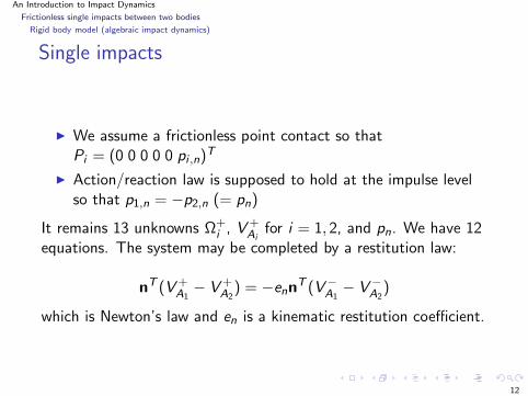
We assume a frictionless point contact so thatPi = (0 0 0 0 0 pi ,n)
T
Action/reaction law is supposed to hold at the impulse levelso that p1,n = −p2,n (= pn)
It remains 13 unknowns Ω+i , V +
Aifor i = 1, 2, and pn. We have 12
equations. The system may be completed by a restitution law:
nT (V +A1
− V +A2
) = −ennT (V−
A1− V−
A2)
which is Newton’s law and en is a kinematic restitution coefficient.
12
An Introduction to Impact Dynamics
Frictionless single impacts between two bodies
Rigid body model (algebraic impact dynamics)
Single impacts
Notice that if MAiis not diagonal (inertial couplings between
normal and tangential directions) then even without friction ortangential deformation one may have jumps in Ωi and Vt,Ai
.
The system is solvable with a unique post-impact velocity and aunique impulse with Newton’s rule of impact.
The kinetic energy loss is given by:
TL =1
2
m1m2
m1 + m2(e2
n − 1)(nT (V−A1
− V−A2
))2
that is ≤ 0 for all e2 ≤ 1. Since nT (V−A1
− V−A2
) < 0 then rebound
implies nT (V +A1
− V +A2
) ≥ 0 so that e ≥ 0: e ∈ [0, 1].
13
An Introduction to Impact Dynamics
Frictionless single impacts between two bodies
Rigid body model (algebraic impact dynamics)
The proof may be done by using Kelvin’s formula which reads
TL =∑
i=1,2
1
2[0 PT
i ](τ+Ai
+ τ−Ai
)
where τAiis the body i twist at the contact point Ai . Since
PTi = (0 0 pn,i ) one obtains
TL =∑
i=1,2
1
2pn,i (v
+n,i + v−
n,i
where nT (VAi= vn,i . Using the impact dynamics
mi (v+n,i − v−
n,i ) = pn,i , pn,1 = −pn,2 and the Netwon’s impact lawthe result follows.
14
An Introduction to Impact Dynamics
Frictionless single impacts between two bodies
Rigid body model (Darboux-Keller’s impact dynamics)
Single impacts
Let us turn our attention to the Darboux-Keller dynamics ofimpact.
Three main definitions of the restitution coefficient:
Kinematic (Newton)
Kinetic (Poisson)
Energetic (Stronge, Peres, Boulanger)
Other definitions exist (Ivanov’s ratio of kinetic energies).
Restitution coefficients are a macroscopic model of a complexphenomenon involving local and global effects of the two bodiesthat collide each other.
15
An Introduction to Impact Dynamics
Frictionless single impacts between two bodies
Rigid body model (Darboux-Keller’s impact dynamics)
Single impacts
The Darboux-Keller model is based on some assumptions:
Positions q remain constant during the shock
There is no tangential compliance
All other forces than the impact ones are negligible
The collision consists of a compression phase followed by anexpansion phase
These assumptions may not be verified, as well as the fact that theimpact is instantaneous, or that it should not create kinetic energy(vibrating bodies that collide may “create” energy at the impactmacroscopic level...).
This is an extension of Routh’s graphical method that applies to2D impacts only.
16
An Introduction to Impact Dynamics
Frictionless single impacts between two bodies
Rigid body model (Darboux-Keller’s impact dynamics)
Single impacts
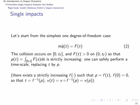
Let’s start from the simplest one degree-of-freedom case:
mq(t) = F (t) (2)
The collision occurs on [0, tf ], and F (t) > 0 on (0, tf ) so thatp(t) =
∫
[0,t] F (s)ds is strictly increasing: one can safely perform atime-scale, replacing t by p.
(there exists a strictly increasing f (·) such that p = f (t), f (0) = 0,so that t = f −1(p), v(t) = v f −1(p) = v(p)).
17
An Introduction to Impact Dynamics
Frictionless single impacts between two bodies
Rigid body model (Darboux-Keller’s impact dynamics)
Single impacts
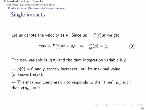
Let us denote the velocity as v . Since dp = F (t)dt we get:
mdv = F (t)dt = dp ⇔ dvdp
(p) = 1m (3)
The new variable is v(p) and the dum integration variable is p:
p(0) = 0 and p strictly increases until its maximal value(unknown) p(tf ).
The maximal compression corresponds to the “time” ptc suchthat v(ptc ) = 0.
18
An Introduction to Impact Dynamics
Frictionless single impacts between two bodies
Rigid body model (Darboux-Keller’s impact dynamics)
Single impacts
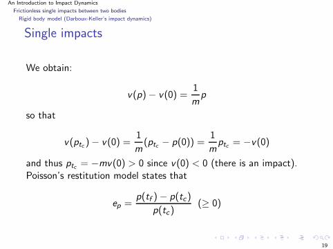
We obtain:
v(p) − v(0) =1
mp
so that
v(ptc ) − v(0) =1
m(ptc − p(0)) =
1
mptc = −v(0)
and thus ptc = −mv(0) > 0 since v(0) < 0 (there is an impact).Poisson’s restitution model states that
ep =p(tf ) − p(tc)
p(tc)(≥ 0)
19
An Introduction to Impact Dynamics
Frictionless single impacts between two bodies
Rigid body model (Darboux-Keller’s impact dynamics)
Single impacts
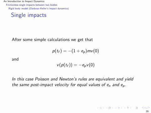
After some simple calculations we get that
p(tf ) = −(1 + ep)mv(0)
andv(p(tf )) = −epv(0)
In this case Poisson and Newton’s rules are equivalent and yieldthe same post-impact velocity for equal values of en and ep.
20

An Introduction to Impact Dynamics
Frictionless single impacts between two bodies
Rigid body model (Darboux-Keller’s impact dynamics)
Single impacts
The energetic model of restitution (Stronge) states that:
e2∗ =
elastic energy released during the expansion phase
elastic energy released during the compression phase
and is found to be equal to
e2∗ = −Wn,e
Wn,c(≥ 0)
where
Wn,e =
∫
[p(tc ),p(tf )]v(p)dp, Wn,c =
∫
[0,p(tc )]v(p)dp
are the works performed by the normal force during the expansionphase (resp. compression phase).(it was used that F (t)v(t)dt = v(p)dp, and due to infinite tangential
stiffnesses the elastic energy is entirely due to the normal deformation).21
An Introduction to Impact Dynamics
Frictionless single impacts between two bodies
Rigid body model (Darboux-Keller’s impact dynamics)
Single impacts
One computes (recall that v(p(tc)) = 0):
Wn,e =1
2v2(p(tf )) and Wn,c =
1
2(−v2(0))
so that
e2∗ =
v2(p(tf ))
v2(0)and v(p(tf )) = −e∗v(0)
(since v(0) < 0, v(p(tf )) > 0 and e∗ ≥ 0).
Again in such a simple case the energetical and the kinematic(Newton) laws are equivalent and provide the same impactoutcome for e∗ = en.
22
An Introduction to Impact Dynamics
Frictionless single impacts between two bodies
Rigid body model (Darboux-Keller’s impact dynamics)
Single impacts
It easily follows that the loss of kinetic energy is given by
TL = T+ − T− =1
2m(e2 − 1)v2(0) (4)
so that TL ≤ 0 ⇒ e ∈ [−1, 1].
Then the final velocity admissibility states that v(tf ) ≥ 0 whichimplies since v(0) < 0 that e ≥ 0. We conclude that
e ∈ [0, 1]
But such bounds will not always be true in more complex collisions(friction, multiple impacts).
23

An Introduction to Impact Dynamics
Frictionless single impacts between two bodies
Comparison of the three coefficients
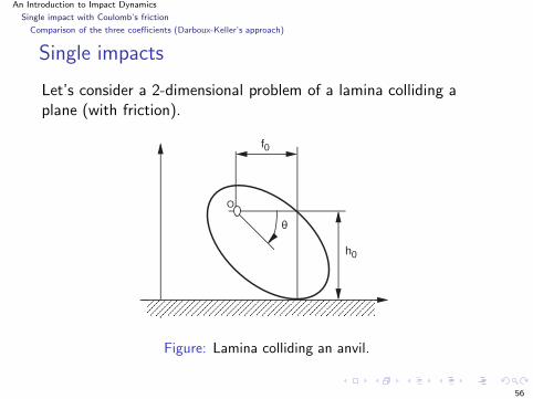
Single impacts
In the previous one degree-of-freedom case all three coefficients areequal. Let’s consider a 2-dimensional problem of a lamina collidinga plane (without friction).
O
θ
f0
h0
AAAAAAAAAAAAAAAAAAAAAAAAAAAAAAAAAAAAAAAAAA
Figure: Lamina colliding an anvil.
24
An Introduction to Impact Dynamics
Frictionless single impacts between two bodies
Comparison of the three coefficients
Single impacts
The kinematics at the contact point yields:
vn = f0θ and vt = h0θ
so that in particular if f0 and h0 6= 0 one has
vn(p(tc)) = 0 ⇒ vt(p(tc )) = 0 :
sliding vanishes when compression ends. So from the basicassumptions the collision is:
(compression vn < 0 + sliding vt > 0)
followed by
(expansion vn > 0 + sliding vt < 0 )
25
An Introduction to Impact Dynamics
Frictionless single impacts between two bodies
Comparison of the three coefficients
Single impacts
Newton’s law: vn(tf ) = −envn(0) so that vt(tf ) = −envt(0)and θ(tf ) = −enθ(0).
Poisson’s law: Let I be the moment of inertia of the laminaw.r.t. the rotating point O. Then after integration over thecompresion and expansion phases:
I (θ(pn(tf )) − θ(0)) = f0pn(tf )
while pn(tc) = −I θ(0). So ep = p(tf )−p(tc )p(tc )
= − θ(p(tf ))
θ(0)= en.
26
An Introduction to Impact Dynamics
Frictionless single impacts between two bodies
Comparison of the three coefficients
Single impacts
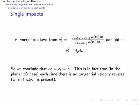
Energetical law: from e2∗ = −
R
[pn(tf ),pn(tc )] vn(pn)dpnR
[0,pn (tc )]vn(pn)dpn
one obtains:
e2∗ = epen
So we conclude that en = ep = e∗. This is in fact true (in theplanar 2D case) each time there is no tangential velocity reversal(when friction is present).
27
An Introduction to Impact Dynamics
Single impact with Coulomb’s friction
Single impacts
Let us now pass to the case where friction is present during thecollision between two bodies.
28
An Introduction to Impact Dynamics
Single impact with Coulomb’s friction
Friction at the impulse level
Single impacts
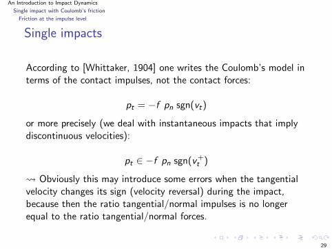
According to [Whittaker, 1904] one writes the Coulomb’s model interms of the contact impulses, not the contact forces:
pt = −f pn sgn(vt)
or more precisely (we deal with instantaneous impacts that implydiscontinuous velocities):
pt ∈ −f pn sgn(v+t )
Obviously this may introduce some errors when the tangentialvelocity changes its sign (velocity reversal) during the impact,because then the ratio tangential/normal impulses is no longerequal to the ratio tangential/normal forces.
29

An Introduction to Impact Dynamics
Single impact with Coulomb’s friction
Friction at the impulse level
Indeed:
TO BE DONE
30
An Introduction to Impact Dynamics
Single impact with Coulomb’s friction
Friction at the impulse level
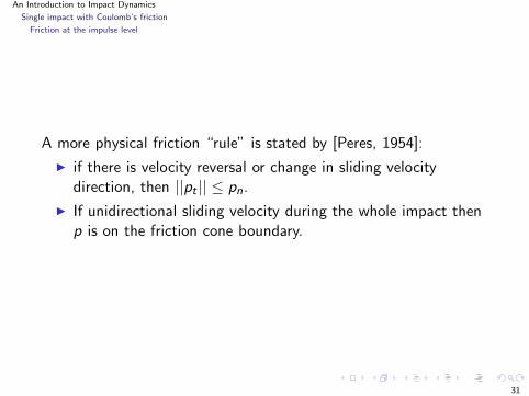
A more physical friction “rule” is stated by [Peres, 1954]:
if there is velocity reversal or change in sliding velocitydirection, then ||pt || ≤ pn.
If unidirectional sliding velocity during the whole impact thenp is on the friction cone boundary.
31
An Introduction to Impact Dynamics
Single impact with Coulomb’s friction
Friction at the impulse level
Single impacts
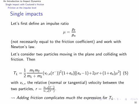
Let’s first define an impulse ratio
µ =pt
pn
(not necessarily equal to the friction coefficient) and work withNewton’s law.
Let’s consider two particles moving in the plane and colliding withfriction. Then
TL =1
2
m1m2
m1 + m2(vr ,n(t
−))2(1+en)[(en−1)+2µr+(1+en)µ2] (5)
with vr ,∗ the relative (normal or tangential) velocity between the
two particles, r =vr,t(t−)vr,n(t−) .
Adding friction complicates much the expression for TL.32
An Introduction to Impact Dynamics
Single impact with Coulomb’s friction
Friction at the impulse level
Single impacts
The case of a particle against a wall
The impact dynamics is
m(v+ − v−) = m
v+t − v−
t
v+n − v−
n
=
pt
pn
Let’s trypt = −f pn sgn(v+
t )
with f > 0, and
v+n = −env
−n , v−
n < 0
33
An Introduction to Impact Dynamics
Single impact with Coulomb’s friction
Friction at the impulse level
Single impacts
Simple calculations yield:
pn = −m(1 + en)v−n > 0
v+t − v−
t = f (1 + en)v−n sgn(v+
t )(6)
so we have to solve a generalized equation to compute v+t . This
boils down to computing the intersection between the graph of themultifunction
v+t 7→ f (1 + en)v
−n sgn(v+
t )
and the single-valued function
v+t 7→ v+
t − v−t
34
An Introduction to Impact Dynamics
Single impact with Coulomb’s friction
Friction at the impulse level
Single impacts
There are three possible cases:
v−t < 0 and v−
t < f (1 + en)v−n : then v+
t < 0 andv+t = −f (1 + en)v
−n + v−
t and pt = fpn.
v−t > 0 and v−
t > −f (1 + en)v−n : then v+
t > 0 andv+t = f (1 + en)v
−n + v−
t and pt = −fpn.
|v−t | ≤ f (1 + en)|v−
n |, then v+t = 0 and |pt | ≤ fpn.
The model tells us that there may be slipping v−t 6= 0 followed by
sticking v+t = 0.
35
An Introduction to Impact Dynamics
Single impact with Coulomb’s friction
Friction at the impulse level
Single impacts
In the above case there is a unique solution for v+t because
the sign multifunction is maximal monotone so thegeneralized equation has a unique solution.
The generalized equation for v+t is simple and monotone
because of no inertial couplings between the normal andtangential directions.
Easy calculations show that for en ∈ [0, 1] one has TL ≤ 0 forall v−
t and v−n because of decoupling, and |v+
t | ≤ |v−t |.
36
An Introduction to Impact Dynamics
Single impact with Coulomb’s friction
Friction at the impulse level
Single impacts
Let’s try an “explicit” way: pt = −f pnsgn(v−t ), then we obtain:
v+t = v−
t + f (1 + e)v−n sgn(v−
t )
Let v−t > 0, then v+
t = f (1 + e)v−n + v−
t and the sign of v+t
depends on f , e and the pre-impact normal velocity magnitude: isthere some sound mechanical behaviour behind this?
Moreover v−t = 0 implies v+
t ∈ f (1 + e)|v−n |[−1, 1], so the
mapping is multivalued (no single value of the post-impactvelocity) and the energetical behaviour is not clear.
It is always better to work with implicit formulations of theunilateral inclusions.
37
An Introduction to Impact Dynamics
Single impact with Coulomb’s friction
Friction at the impulse level
Single impacts
The effect of inertial couplings
Let’s consider a rod falling on the ground. The dynamics is givenby, with q = (x , y , θ)T :
mq =
0−mg
0
+
01
l sin(θ)
λn +
10
l cos(θ)
λt (7)
where the contact force is λ = (λt , λn)T ,
0 ≤ λn ⊥ h(q) = y − l cos(θ) ≥ 0
λt = −f λnsgn(x + l θ sin(θ))
38
An Introduction to Impact Dynamics
Single impact with Coulomb’s friction
Friction at the impulse level
Single impacts
The impact dynamics is deduced as:
m(x+ − x−) = pt
m(y+ − y−) = pn
m(θ+ − θ−) = l sin(θ)pn + l cos(θ)pt
y+ + l θ+ sin(θ) = −e(y− + l θ− sin(θ))
pt = −fpnsgn(x+ + l θ+ cos(θ))
pn ≥ 0, y− + l θ− sin(θ) ≤ 0, y+ + l θ+ sin(θ) ≥ 0
(8)
which we may see as a generalized equation to be solved with thedata (x−, y−, θ−) and e, f , with unknowns (x+, y+, θ+) and pn,pt .
39
An Introduction to Impact Dynamics
Single impact with Coulomb’s friction
Friction at the impulse level
Single impacts
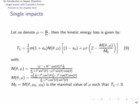
Let us denote µ = pt
pn, then the kinetic energy loss is given by:
TL =1
2m(1 + en)N(θ, µ)
[
(1 − en) + µr
(
2 − M(θ, µ)
M0
)]
(9)
with:
N(θ, µ) =(y−+l θ− sin(θ))2 I
mIm
+l2 sin2(θ)−µl2 sin(θ) cos(θ)
M(θ, µ) =µ( I
m+l2 cos2(θ))−l2 cos(θ) sin(θ)
Im
+l4 cos2(θ) sin2(θ)
M0 = M(θ, µ0, µ0) is the maximal value of µ such that TL < 0.
40
An Introduction to Impact Dynamics
Single impact with Coulomb’s friction
Friction at the impulse level
Single impacts
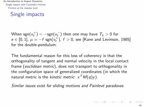
When sgn(v+t ) = −sgn(v−
t ) then one may have TL > 0 fore ∈ [0, 1], µ = −f sgn(v+
t ), f > 0, see [Kane and Levinson, 1985]for the double-pendulum.
The fundamental reason for this loss of coherency is that theorthogonality of tangent and normal velocity in the local contactframe (euclidean metric), does not transport to orthogonality inthe configuration space of generalized coordinates (in which thenatural metric is the kinetic metric: xTM(q)y).
Similar issues exist for sliding motions and Painleve paradoxes.
41
An Introduction to Impact Dynamics
Single impact with Coulomb’s friction
Friction at the impulse level
Single impacts
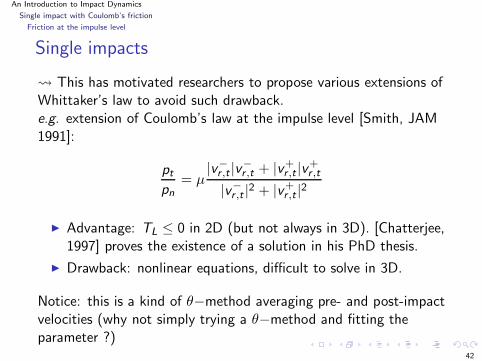
This has motivated researchers to propose various extensions ofWhittaker’s law to avoid such drawback.e.g. extension of Coulomb’s law at the impulse level [Smith, JAM1991]:
pt
pn
= µ|v−
r ,t |v−r ,t + |v+
r ,t |v+r ,t
|v−r ,t |2 + |v+
r ,t |2
Advantage: TL ≤ 0 in 2D (but not always in 3D). [Chatterjee,1997] proves the existence of a solution in his PhD thesis.
Drawback: nonlinear equations, difficult to solve in 3D.
Notice: this is a kind of θ−method averaging pre- and post-impactvelocities (why not simply trying a θ−method and fitting theparameter ?)
42
An Introduction to Impact Dynamics
Single impact with Coulomb’s friction
The impulse ratio
Single impacts
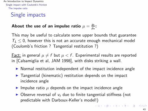
About the use of an impulse ratio µ = pt
pn:
This may be useful to calculate some upper bounds that guaranteeTL ≤ 0, however this is not an accurate enough mechanical model(Coulomb’s friction ? Tangential restitution ?)
Fact: in general µ 6= f but µ < f . Experimental results are reportedin [Calsamiglia et al, JAM 1998], with disks striking a wall.
Normal restitution independent of the impact incidence angle
Tangential (kinematic) restitution depends on the impactincidence angle
Impulse ratio µ depends on the impact incidence angle
Observe reversal of vt due to finite tangential stiffness (notpredictable with Darboux-Keller’s model!)
43
An Introduction to Impact Dynamics
Single impact with Coulomb’s friction
The impulse ratio
Single impacts
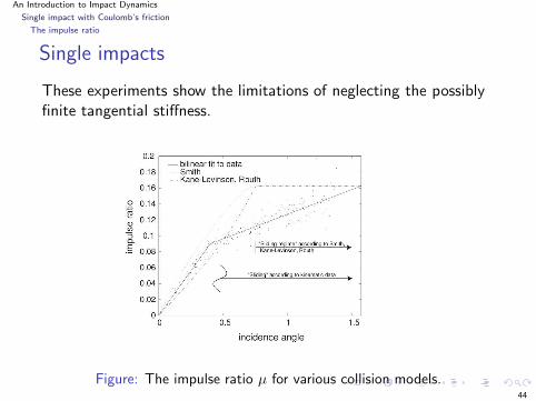
These experiments show the limitations of neglecting the possiblyfinite tangential stiffness.
Figure: The impulse ratio µ for various collision models.44

An Introduction to Impact Dynamics
Single impact with Coulomb’s friction
The impulse ratio
Single impacts
The experimental results disks colliding a wall in [Calsamiglia et alJAM 1998] show that even in the case of spheres/disks where the“basic” (en, f ) law of Whittaker is mathematically sound andassures TL ≤ 0, it may be too poor to correctly represent theimpact phenomenon at a reasonable degree of realism.
So even for the simplest cases this law satisfies the requirements(a) (b) and (c) but fails to satisfy (d) and (e).
45
An Introduction to Impact Dynamics
Single impact with Coulomb’s friction
The impulse ratio
Single impacts
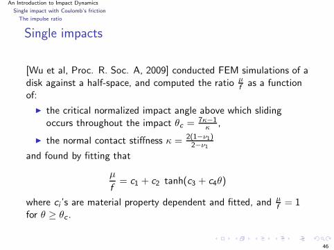
[Wu et al, Proc. R. Soc. A, 2009] conducted FEM simulations of adisk against a half-space, and computed the ratio µ
fas a function
of:
the critical normalized impact angle above which slidingoccurs throughout the impact θc = 7κ−1
κ ,
the normal contact stiffness κ = 2(1−ν1)2−ν1
and found by fitting that
µ
f= c1 + c2 tanh(c3 + c4θ)
where ci ’s are material property dependent and fitted, and µf
= 1for θ ≥ θc .
46
An Introduction to Impact Dynamics
Single impact with Coulomb’s friction
Kinematic tangential restitution
Single impacts
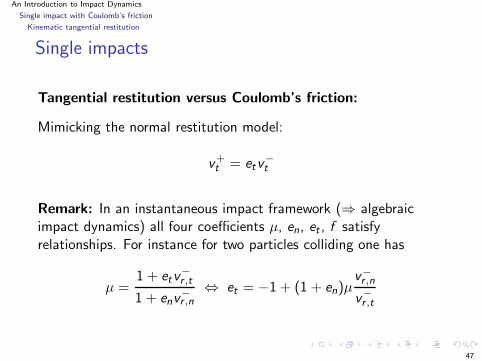
Tangential restitution versus Coulomb’s friction:
Mimicking the normal restitution model:
v+t = etv
−t
Remark: In an instantaneous impact framework (⇒ algebraicimpact dynamics) all four coefficients µ, en, et , f satisfyrelationships. For instance for two particles colliding one has
µ =1 + etv
−r ,t
1 + env−r ,n
⇔ et = −1 + (1 + en)µv−r ,n
v−r ,t
47

An Introduction to Impact Dynamics
Single impact with Coulomb’s friction
Kinematic tangential restitution
Single impacts
Physical meaning of et :
Can et be independent of friction ? ( no friction ⇒ notangential deformation!)
How can one mix et and f into a single tangential rule ?
48
An Introduction to Impact Dynamics
Single impact with Coulomb’s friction
Kinematic tangential restitution
Single impacts
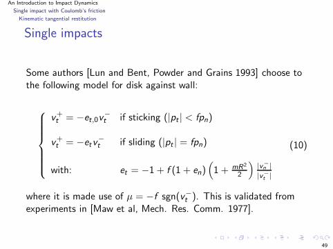
Some authors [Lun and Bent, Powder and Grains 1993] choose tothe following model for disk against wall:
v+t = −et,0v
−t if sticking (|pt | < fpn)
v+t = −etv
−t if sliding (|pt | = fpn)
with: et = −1 + f (1 + en)(
1 + mR2
2
)
|v−
n ||v−
t |
(10)
where it is made use of µ = −f sgn(v−t ). This is validated from
experiments in [Maw et al, Mech. Res. Comm. 1977].
49

An Introduction to Impact Dynamics
Single impact with Coulomb’s friction
Kinematic tangential restitution
The works of Maw, Barber and Fawcett 1976, 1977, 1981, thatevidence the role of Coulomb friction, stick, slip, and the incidenceangle.
TO BE DONE
50
An Introduction to Impact Dynamics
Single impact with Coulomb’s friction
Kinematic tangential restitution
Single impacts
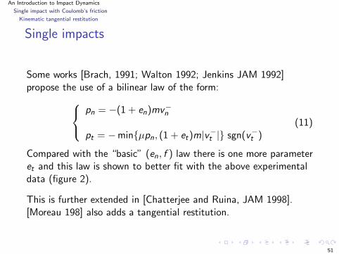
Some works [Brach, 1991; Walton 1992; Jenkins JAM 1992]propose the use of a bilinear law of the form:
pn = −(1 + en)mv−n
pt = −minµpn, (1 + et)m|v−t | sgn(v−
t )(11)
Compared with the “basic” (en, f ) law there is one more parameteret and this law is shown to better fit with the above experimentaldata (figure 2).
This is further extended in [Chatterjee and Ruina, JAM 1998].[Moreau 198] also adds a tangential restitution.
51
An Introduction to Impact Dynamics
Single impact with Coulomb’s friction
Kinematic tangential restitution
Single impacts
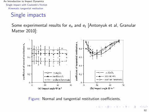
Some experimental results for en and et [Antonyuk et al, GranularMatter 2010]:
Figure: Normal and tangential restitution coefficients.
52
An Introduction to Impact Dynamics
Single impact with Coulomb’s friction
Kinematic tangential restitution
The friction coefficient during the impact may depend on theinitial tangential velocity magnitude |vt | [Garland and Rogers, JAM2009].
TO BE DONE
53
An Introduction to Impact Dynamics
Single impact with Coulomb’s friction
Kinematic tangential restitution
Single impacts
Those analytical and experimental results indicate that: The normal deformation process is independent of the
tangential one (impact angle varied from 0 to 80 degrees)confirming other experiments [Calsamiglia et al, JAM 1998].
The tangential restitution coefficient varies with the impactangle (transitions from rolling without slipping, to sliding atlarge angles), which demonstrates that Coulomb’s likephenomena are behind it (so et is a “super-macroscopic”coefficient!).
For sphere/sphere or sphere/plane oblique impacts, f mayvary with |vt .
The problem raised by inertial couplings and Kane-Levinson’sexample with TL > 0 is a fundamental issue: one can estimateseparately en and f from suitable experiments, but insertingthem into the Whittaker’s law of impact with friction nolonger works: the physical validity of en and f seems to be 54

An Introduction to Impact Dynamics
Single impact with Coulomb’s friction
Kinematic tangential restitution
Single impacts
The underlying issue is that using Newton’s coefficient andCoulomb’s friction model at the impulse level does not yield ageneralized equation for the post-impact velocities, with goodproperties like maximal monotonicity (that would assure existenceand uniqueness of the solutions).This has motivated researchers to use other approaches:
Fremond: recast such laws into a general framework inspiredby Moreau’s superpotentials (problem: not easy to discoverthe right superpotential function so that the resulting law hasgood parameters)
or:
Darboux-Keller’s approach with Poisson’s or Stronge’s(energetic) coefficients.
55
An Introduction to Impact Dynamics
Single impact with Coulomb’s friction
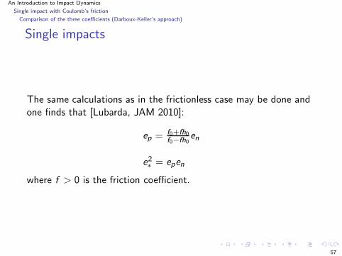
Comparison of the three coefficients (Darboux-Keller’s approach)
Single impacts
Let’s consider a 2-dimensional problem of a lamina colliding aplane (with friction).
O
θ
f0
h0
AAAAAAAAAAAAAAAAAAAAAAAAAAAAAAAAAAAAAAAAAA
Figure: Lamina colliding an anvil.
56
An Introduction to Impact Dynamics
Single impact with Coulomb’s friction
Comparison of the three coefficients (Darboux-Keller’s approach)
Single impacts
The same calculations as in the frictionless case may be done andone finds that [Lubarda, JAM 2010]:
ep = f0+fh0f0−fh0
en
e2∗ = epen
where f > 0 is the friction coefficient.
57
An Introduction to Impact Dynamics
Single impact with Coulomb’s friction
Comparison of the three coefficients (Darboux-Keller’s approach)
Single impacts
It is then easily calculated that ep =(
f0+fh0f0−fh0
) 12e∗ and
en =(
f0−fh0f0+fh0
)12e∗, so that:
en < e∗ < ep (12)
(provided of course that f0 − fh0 > 0 ⇔ en > 0 (there is arebound after the impact))
58

An Introduction to Impact Dynamics
Single impact with Coulomb’s friction
Bounds on the restitution coefficients
Single impacts
The loss of kinetic energy is given by:
TL = 12 I (θ2(p(tf )) − θ2(0)) = 1
2 I (e2n − 1)θ2(0)
= 12 I θ2(0)
(
1 − e2p
(f0−fh0)2
(f0+fh0)2
)
(13)
from which one deduces that en ≤ 1. Then from the aboverelationships between both coefficients: ep ≤ f0+fh0
f0−fh0.
59
An Introduction to Impact Dynamics
Single impact with Coulomb’s friction
Bounds on the restitution coefficients
Single impacts
By construction of the energetical coefficient one has necessarilye∗ ≤ 1 (which is the advantage of using it). The above upperbounds may then be refined:
ep ≤(
1 +2fh0
f0 − fh0
)2
(larger than 1 upper bound) and
en ≤(
1 − 2fh0
f0 − fh0
)2
(smaller than 1 upper bound, confirms that infinite tangentialstiffness may be a limitation of the model)
60
An Introduction to Impact Dynamics
Single impact with Coulomb’s friction
Bounds on the restitution coefficients
Single impacts
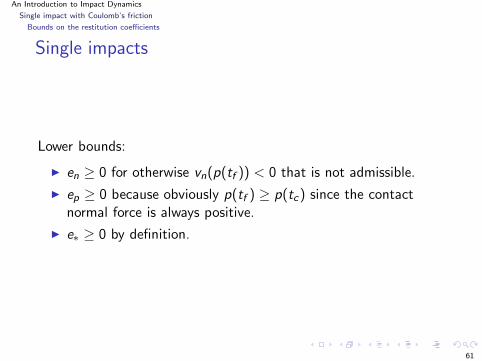
Lower bounds:
en ≥ 0 for otherwise vn(p(tf )) < 0 that is not admissible.
ep ≥ 0 because obviously p(tf ) ≥ p(tc) since the contactnormal force is always positive.
e∗ ≥ 0 by definition.
61
An Introduction to Impact Dynamics
Single impact with Coulomb’s friction
The tangential restitution
Single impacts
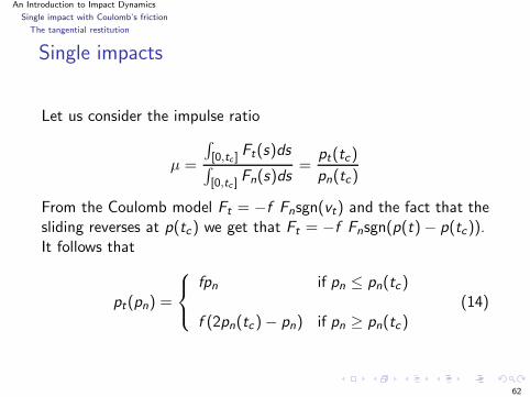
Let us consider the impulse ratio
µ =
∫
[0,tc ]Ft(s)ds
∫
[0,tc ]Fn(s)ds
=pt(tc)
pn(tc)
From the Coulomb model Ft = −f Fnsgn(vt) and the fact that thesliding reverses at p(tc) we get that Ft = −f Fnsgn(p(t) − p(tc)).It follows that
pt(pn) =
fpn if pn ≤ pn(tc )
f (2pn(tc ) − pn) if pn ≥ pn(tc )(14)
62
An Introduction to Impact Dynamics
Single impact with Coulomb’s friction
The tangential restitution
Single impacts
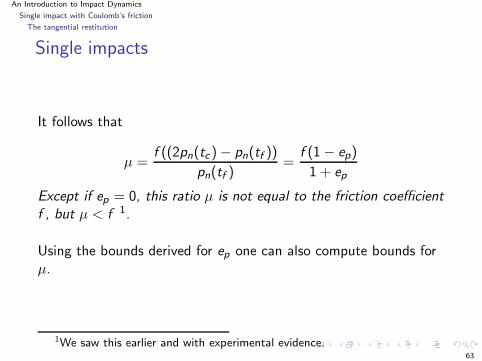
It follows that
µ =f ((2pn(tc ) − pn(tf ))
pn(tf )=
f (1 − ep)
1 + ep
Except if ep = 0, this ratio µ is not equal to the friction coefficientf , but µ < f 1.
Using the bounds derived for ep one can also compute bounds forµ.
1We saw this earlier and with experimental evidence.63
An Introduction to Impact Dynamics
Single impact with Coulomb’s friction
The tangential restitution
Single impacts
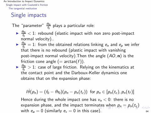
The “parameter” fh0f0
plays a particular role:
fh0f0
< 1: rebound (elastic impact with non zero post-impactnormal velocity)..
fh0f0
= 1: from the obtained relations linking en and ep we inferthat there is no rebound (plastic impact with vanishingpost-impact normal velocity).Then the angle (AO,n) is thefriction cone angle (= arctan(f )).
fh0f0
> 1: case of large friction. Relying on the kinematics atthe contact point and the Darboux-Keller dynamics oneobtains that on the expansion phase:
I θ(pn) = (f0 − fh0)(pn − pn(tc)) for pn ∈ [pn(tc), pn(tf )]
Hence during the whole impact one has vn < 0: there is noexpansion phase, and the impact terminates when pn = pn(tc)with ep = 0 (similarly e∗ = 0 in this case). 64
An Introduction to Impact Dynamics
Single impact with Coulomb’s friction
Conclusions (2D impact)
Single impacts
Relying on the Darboux-Keller approach one can deriverelationships between the three most well-known restitutioncoefficients, as well as bounds from kinetic energy constraintsand post-impact velocity admissibility.
The advantage of the energetical coefficient is that it isintrinsically (under the stated assumptions) inside [0, 1].
The tangential frictional effects influence the normal ones inthe sense that if friction is large enough (the friction cone“contains” the center of rotation) then the impact is plastic.
Notice that until now we made no particular assumption onthe type of contact model (viscoelastic, viscoplastic,elastoplastic..). The normal coefficient of restitutionencapsulates all kinds of energy losses (but not the tangentialstiffness!).
65
An Introduction to Impact Dynamics
Single impact with Coulomb’s friction
Conclusions (2D impact)
Single impacts
Logically, impacts with friction should be prone to the samedifficulties as sliding motion with friction (frictional paroxisms forsome configurations).
However some of the Painleve paradox effects may not exist inshock dynamics since one works with impulses and not forces: asshown in [Genot and Brogliato, EJM A/Solids 1998] at somepoints of the (θ, θ) plane, Fn → ∞ while its impulse pn < ∞.
We retrieve here a big advantage of working with impulses,similarly to what happens in time-stepping schemes a laMoreau-Jean.
66
An Introduction to Impact Dynamics
Darboux-Keller’s dynamics: the 3D case
Single impacts
Proceeding in the same way, the case of two bodies colliding withCoulomb friction gives the dynamics:
dvr,n
dpndvr,t1dpn
dvr,t2dpn
= M−1
−f cos(ζ)−f sin(ζ)
1
(15)
where ζ is the angle between the two tangential velocities in thelocal contact frame, the mass matrix inverse is given by expressionsof the form:
m−111 =
∑
i=1,2
−r23i I
−1i ,12 + r3i r1i I
−1i ,32 + r3i r2i I
−1i ,13 − r2i r1i I
−1i ,33
with AiGi = (r1i r2i r3i )T in the local frame.
67
An Introduction to Impact Dynamics
Darboux-Keller’s dynamics: the 3D case
Single impacts
The 3D case is much more involved. Darboux in his 1880 paperstates some results:
Proposition
If during a soft shock process a sliding phase ends, and if slidingresumes before the end of the collision, then the direction andorientation of the relative tangential velocity on this subsequentperiod is constant.
This of course relies on the above stringent assumptions on theimpact behaviour...
To the best of the speaker’s knowledge, no experimental resultsexist that corroborate any of the studies on Darboux-Keller’s ap-proach...which is somewhat worrying...
68
An Introduction to Impact Dynamics
Darboux-Keller’s dynamics: the 3D case
Geometrical analysis of the impact laws (impulse space)
Single impacts
One desirable property of an impact law is that it should be able tocover all possible admissible post-impact outcomes, under threemain constraints:.
Loss of kinetic energy,
Admissible post-impact velocity,
Impulse inside the friction cone.
69

An Introduction to Impact Dynamics
Darboux-Keller’s dynamics: the 3D case
Geometrical analysis of the impact laws (impulse space)
Analysis of the impact process in the impulse space
70

An Introduction to Impact Dynamics
Darboux-Keller’s dynamics: the 3D case
Geometrical analysis of the impact laws (impulse space)
Single impacts
Figure: Impulse space, allowable impulses.
See Chatterjee’s PhD thesis for a comparison of various above impact
laws in terms of reachable admissible points in the impulse space.71
An Introduction to Impact Dynamics
Darboux-Keller’s dynamics: the 3D case
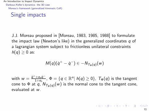
Moreau’s framework (generalized kinematic CoR)
Single impacts
J.J. Moreau proposed in [Moreau, 1983, 1985, 1988] to formulatethe impact law (Newton’s like) in the generalized coordinates q ofa lagrangian system subject to frictionless unilateral constraintsh(q) ≥ 0 as:
M(q)(q+ − q−) ∈ −NTΦ(q)(w)
with w = q++enq−
1+en, Φ = q ∈ R
n| h(q) ≥ 0, TΦ(q) is the tangentcone to Φ at q, NTΦ(q)(w) is the normal cone to the tangent cone,evaluated at w .
72
An Introduction to Impact Dynamics
Darboux-Keller’s dynamics: the 3D case
Moreau’s framework (generalized kinematic CoR)
Single impacts
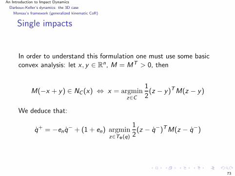
In order to understand this formulation one must use some basicconvex analysis: let x , y ∈ R
n, M = MT > 0, then
M(−x + y) ∈ NC (x) ⇔ x = argminz∈C
1
2(z − y)TM(z − y)
We deduce that:
q+ = −enq− + (1 + en) argmin
z∈TΦ(q)
1
2(z − q−)TM(z − q−)
73
An Introduction to Impact Dynamics
Darboux-Keller’s dynamics: the 3D case
Moreau’s framework (generalized kinematic CoR)
Single impacts
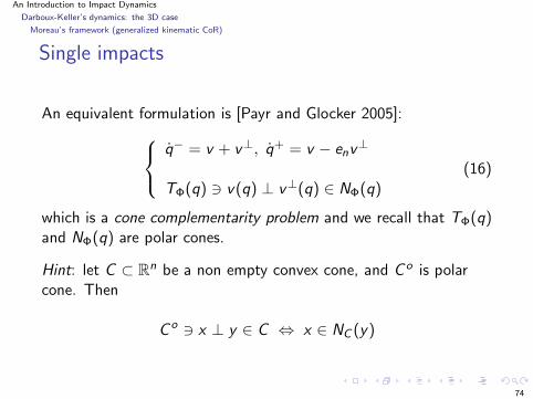
An equivalent formulation is [Payr and Glocker 2005]:
q− = v + v⊥, q+ = v − env⊥
TΦ(q) ∋ v(q) ⊥ v⊥(q) ∈ NΦ(q)(16)
which is a cone complementarity problem and we recall that TΦ(q)and NΦ(q) are polar cones.
Hint: let C ⊂ Rn be a non empty convex cone, and C o is polar
cone. Then
C o ∋ x ⊥ y ∈ C ⇔ x ∈ NC (y)
74
An Introduction to Impact Dynamics
Darboux-Keller’s dynamics: the 3D case
Moreau’s framework (generalized kinematic CoR)
From the kinematics constraints
q+ ∈ TΦ(q), q− ∈ −TΦ(q)
one can deduce the lower limit en ≥ 0.
75
An Introduction to Impact Dynamics
Darboux-Keller’s dynamics: the 3D case
Moreau’s framework (generalized kinematic CoR)
Single impacts
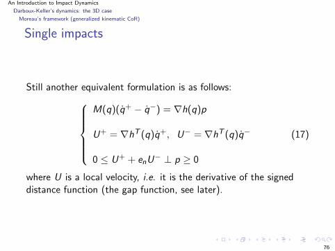
Still another equivalent formulation is as follows:
M(q)(q+ − q−) = ∇h(q)p
U+ = ∇hT (q)q+, U− = ∇hT (q)q−
0 ≤ U+ + enU− ⊥ p ≥ 0
(17)
where U is a local velocity, i.e. it is the derivative of the signeddistance function (the gap function, see later).
76
An Introduction to Impact Dynamics
Darboux-Keller’s dynamics: the 3D case
Moreau’s framework (generalized kinematic CoR)
Single impacts
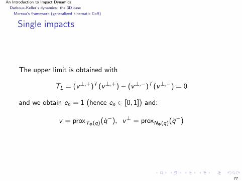
The upper limit is obtained with
TL = (v⊥,+)T (v⊥,+) − (v⊥,−)T (v⊥,−) = 0
and we obtain en = 1 (hence en ∈ [0, 1]) and:
v = proxTΦ(q)(q−), v⊥ = proxNΦ(q)(q
−)
77
An Introduction to Impact Dynamics
Darboux-Keller’s dynamics: the 3D case
Moreau’s framework (generalized kinematic CoR)
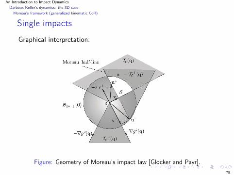
Single impacts
Graphical interpretation:
Figure: Geometry of Moreau’s impact law [Glocker and Payr].
78
An Introduction to Impact Dynamics
Darboux-Keller’s dynamics: the 3D case
Moreau’s framework (generalized kinematic CoR)
Single impacts
Moreau’s framework is formulated for multiple impacts (when theboundary Bd(Φ) has singularities) and therefore provides a clearmathematical framework for frictionless multiple impacts.
This provides a nice and powerful framework however does notfurnish automatically a restitution mapping satisfying all of theabove requirements (in particular the physical meaning of all theparameters in the multiple impact case).
The analysis is also led with Poisson’s CoR in [Payr and Glocker2005].
[Payr and Glocker 2005] analyze various impact rules and extendMoreau’s restitution law to comply with some of the “basic”requirements (like spanning of the whole admissible post-impactvelocity space).
79
An Introduction to Impact Dynamics
Darboux-Keller’s dynamics: the 3D case
First conclusions
Single impacts
The algebraic impact law using en and some tangential restitutionet of f or µ, has been the object of many analysis and extensionsin order improve the basic Whittaker’s law.
All of these models are gross approximations of the impact phenomenon.
It seems difficult to meet all the requirements (even for 2Dimpacts!):
(a) Provide a unique solution for all data
(b) Be numerically tractable
(c) Possess mechanically sound parameters (like restitutioncoefficients)
80

An Introduction to Impact Dynamics
Darboux-Keller’s dynamics: the 3D case
First conclusions
Single impacts
(d) Be able to span the whole subspace of admssiblepost-impact velocities
(e) Be able to correctly predict impact outcomes for varioustypes of bodies (shapes, material) so that it may be validatedthrough experiments.
One always faces the classical problem: add more coefficients atthe price of not being able to estimate them through simpleexperiments.
The model has to be taylored to the application.
Fitting the parameters may also work!
81

An Introduction to Impact Dynamics
Compliant contacts (spring/dashpot, plasticity)
Single impacts
Let’s now analyse compliant models of contact/impact.
82
An Introduction to Impact Dynamics
Compliant contacts (spring/dashpot, plasticity)
Expressions for the kinematic restitution coefficient
Single impacts
A lot of expressions for en have been proposed, most forsphere/sphere or sphere/plane impacts. They mainly arise from:
linear or nonlinear spring/dashpot models (viscoelastic)
viscoplastic, elasto-plastic, visco-elasto-plastic models
FEM simulations to numerically estimate the restitutioncoefficient
83
An Introduction to Impact Dynamics
Compliant contacts (spring/dashpot, plasticity)
Expressions for the kinematic restitution coefficient
Single impacts
The CoR obtained from a linear spring/daspot modelmδ = −c δ − kδ (sometimes called Kelvin-Voigt):
Termination conditions δ = 0 and δ > 0:
en = exp
(
− απ√1 − α2
)
α = c
2√
km.
Positive total impulse, however Fn < 0 during the collision!
84

An Introduction to Impact Dynamics
Compliant contacts (spring/dashpot, plasticity)
Expressions for the kinematic restitution coefficient
Single impacts
Figure: Force/identation relation for various spring/dashpots.
85
An Introduction to Impact Dynamics
Compliant contacts (spring/dashpot, plasticity)
Expressions for the kinematic restitution coefficient
Single impacts
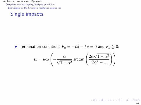
Termination conditions Fn = −c δ − kδ = 0 and Fn ≥ 0:
en = exp
(
− α√1 − α2
arctan
(
2α√
1 − α2
2α2 − 1
))
86

An Introduction to Impact Dynamics
Compliant contacts (spring/dashpot, plasticity)
Expressions for the kinematic restitution coefficient
Single impacts
Notice in passing that complementarity doesn’t mean perfectrigidity, as it can be applied to compliant contact:0 ≤ −Fn(t) + λ(t) ⊥ λ(t) ≥ 0 and mδ(t) = λ(t) that is alinear complementarity system x = Ax + Bλ,0 ≤ λ ⊥ w = Cx + Dλ ≥ 0.
These two models are rather poor since en does not dependon vn(0), contradicting experiments and more sophisticatedanalysis.
Such models may yield stiff ODEs when used in multibodysystems simulations.
Other, similar models made of linear springs and dashpotsexist (like the Zener model), all sharing the same deficiencies.
87
An Introduction to Impact Dynamics
Compliant contacts (spring/dashpot, plasticity)
Expressions for the kinematic restitution coefficient
Single impacts
The compliance relations obtained from Hertz’ theory(statical theory of elastic contact)
Basic assumptions:
the two bodies are at the time of impact in a quasistaticstate, i.e. all the external dynamic loads are taken to be inequilibrium, the contact pressure increases slowly and theanalysis can be based on a static contact theory.
waves in the bodies are neglected, i.e. impact duration ≫propagation time of released elastic waves along the wholelength of each impacted body.
the surfaces in contact are non-conforming surfaces.
88
An Introduction to Impact Dynamics
Compliant contacts (spring/dashpot, plasticity)
Expressions for the kinematic restitution coefficient
Single impacts
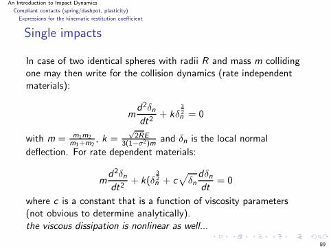
In case of two identical spheres with radii R and mass m collidingone may then write for the collision dynamics (rate independentmaterials):
md2δn
dt2+ kδ
32n = 0
with m = m1m2m1+m2
, k =√
2RE3(1−σ2)m
and δn is the local normal
deflection. For rate dependent materials:
md2δn
dt2+ k(δ
32n + c
√
δndδn
dt= 0
where c is a constant that is a function of viscosity parameters(not obvious to determine analytically).the viscous dissipation is nonlinear as well...
89

An Introduction to Impact Dynamics
Compliant contacts (spring/dashpot, plasticity)
Expressions for the kinematic restitution coefficient
Single impacts
Remark: the widely used (in some fields like robotics) Hunt andCrossley model [Hunt and Crossley, JAM 1975]:
Fn = −c |δ|mδ − kδm
is not deduced from a rigorous Hertz analysis (m = 32 gives a
viscous term c |δ| 32 δ and not c
√δn
˙dδn). It is rather used becauseof its integrability property.
For low velocities it gives en ≈ 1− βvn(0) for some constant β andthus reproduces a general tendency (for some materials) that en
decreases with increasing vn(0) and en = 1 for very small impactvelocity.
90

An Introduction to Impact Dynamics
Compliant contacts (spring/dashpot, plasticity)
Expressions for the kinematic restitution coefficient
Single impacts
The CoR for nonlinear visco-elastic behaviour [Brilliantov et al,Phys. Rev. E 1996]:
en = 1 − b
(
vn(0)
m∗2
)15
with b = 1.15(
3Ad
2
)(
23E ∗√R∗
)25, Ad = 1
3(3η2−η1)2
3η2+2η1
(1−ν2)(1−2ν)Eν2 .
91

An Introduction to Impact Dynamics
Compliant contacts (spring/dashpot, plasticity)
The effect of plasticity on the CoR
Single impacts
According to [Johnson, Contact Mechanics, 1985] the relationFn(δn) for elasto-plastic contact is not precisely defined, so one hasto resort to approximate analysis.
Assumptions:
The mean contact pressure is constant (during plasticdeformation) and equal to 3.0Y where Y is the yield stress insimple compression.
The Hertz relation δn = a2
Ris still valid, where a is the contact
surface radius, R = R1R2R1+R2
.
92
An Introduction to Impact Dynamics
Compliant contacts (spring/dashpot, plasticity)
The effect of plasticity on the CoR
Single impacts
Then
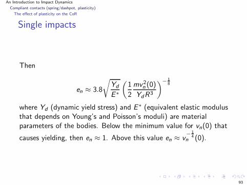
en ≈ 3.8
√
Yd
E ∗
(
1
2
mv2n (0)
YdR3
)− 18
where Yd (dynamic yield stress) and E ∗ (equivalent elastic modulusthat depends on Young’s and Poisson’s moduli) are materialparameters of the bodies. Below the minimum value for vn(0) that
causes yielding, then en ≈ 1. Above this value en ≈ v− 1
4n (0).
93

An Introduction to Impact Dynamics
Compliant contacts (spring/dashpot, plasticity)
The effect of plasticity on the CoR
Single impacts
The obtained value of en in [Johnson, 1985] when compared toexperimental data (steel, aluminium alloy, brass) providesoverestimation of the real CoR.
several subsequent studies to enrich Johnson’s works to bettermatch with experimental measurements.
[Mangwandi et al, Chem. Eng. Sci. 2007] compared variousexpressions of en with experimental measurements with granules(calcium carbonate, polyethylene glycol).
They conclude that the existing results (elastoplastic with full
plasticity during the loading phase [Johnson, 1985]; same but with elastic
contribution during loading [Thorton, 1997]; finite plastic deformation
[Wu et al 2003) yield over- or under-estimation of the CoR.
94
An Introduction to Impact Dynamics
Compliant contacts (spring/dashpot, plasticity)
The effect of plasticity on the CoR
Single impacts
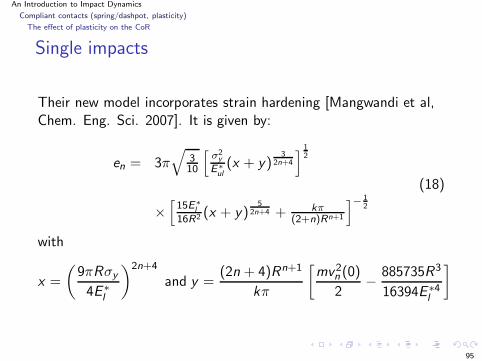
Their new model incorporates strain hardening [Mangwandi et al,Chem. Eng. Sci. 2007]. It is given by:
en = 3π√
310
[
σ2y
E∗
ul(x + y)
32n+4
]12
×[
15E∗
l
16R2 (x + y)5
2n+4 + kπ(2+n)Rn+1
]− 12
(18)
with
x =
(
9πRσy
4E ∗l
)2n+4
and y =(2n + 4)Rn+1
kπ
[
mv2n (0)
2− 885735R3
16394E ∗4l
]
95
An Introduction to Impact Dynamics
Compliant contacts (spring/dashpot, plasticity)
The effect of plasticity on the CoR
Single impacts
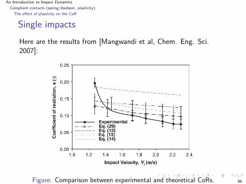
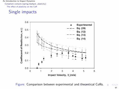
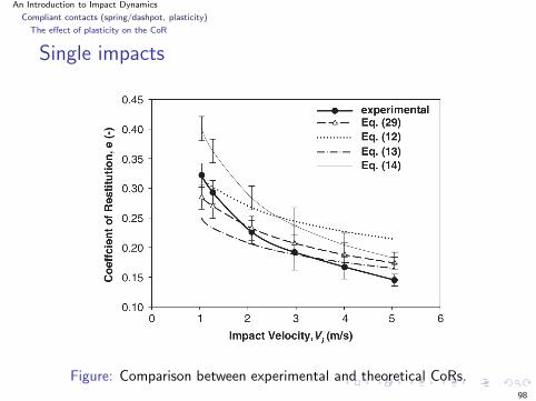
Here are the results from [Mangwandi et al, Chem. Eng. Sci.2007]:
Figure: Comparison between experimental and theoretical CoRs. 96
An Introduction to Impact Dynamics
Compliant contacts (spring/dashpot, plasticity)
The effect of plasticity on the CoR
Single impacts
Figure: Comparison between experimental and theoretical CoRs.97
An Introduction to Impact Dynamics
Compliant contacts (spring/dashpot, plasticity)
The effect of plasticity on the CoR
Single impacts
Figure: Comparison between experimental and theoretical CoRs.98

An Introduction to Impact Dynamics
Compliant contacts (spring/dashpot, plasticity)
The effect of plasticity on the CoR
Single impacts
This raises two fundamental questions:
isn’t it better and more mechanically sound to use Brach’spoint of view (or something similar) with some kind of bilinearmodel and constant coefficients ?
The appeal of such methods is to enable one to calculate en
off-line from material properties (E , ν, geometry). Hoeverwhat is really gained by using such rather awful expressionsfor an impact in so simple conditions (no friction, colinearimpact, sphere/sphere or sphere/plane), since we know thatfriction may drastically change the picture ?
99

An Introduction to Impact Dynamics
Compliant contacts (spring/dashpot, plasticity)
The effect of plasticity on the CoR
Single impacts
Further results:[Steven et al, Powder Techn. 2005] compared 8 definitions of theCoR with experiments of stainless/stainless andchrome-steel/chrome-steel collisions of two spheres:
Linear spring/dashpot with “bad” termination conditions
Hertz contact
Kuwabara and Kono (visco-elastic: Hertz +√
δδ)
Lee and Hermann (Hertz + meff vr ,n)
Walton and Braun (elasto-plastic, bi-stiffness model forloading and unloading phases, constant en)
Walton and Braun (elasto-plastic, bi-stiffness with variable en)
Thorton (elasto-plastic, see above; fitted parameters)
Thorton (elasto-plastic, see above; non-fitted parameters)
100
An Introduction to Impact Dynamics
Compliant contacts (spring/dashpot, plasticity)
The effect of plasticity on the CoR
Single impacts
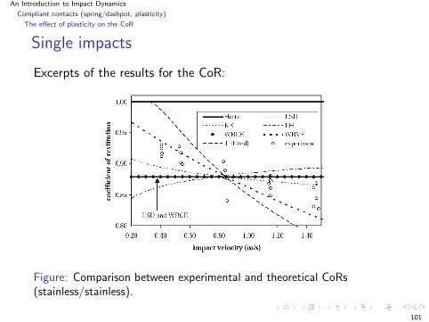
Excerpts of the results for the CoR:
Figure: Comparison between experimental and theoretical CoRs(stainless/stainless).
101
An Introduction to Impact Dynamics
Compliant contacts (spring/dashpot, plasticity)
The effect of plasticity on the CoR
Single impacts
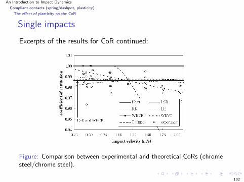
Excerpts of the results for CoR continued:
Figure: Comparison between experimental and theoretical CoRs (chromesteel/chrome steel).
102
An Introduction to Impact Dynamics
Compliant contacts (spring/dashpot, plasticity)
The effect of plasticity on the CoR
Single impacts
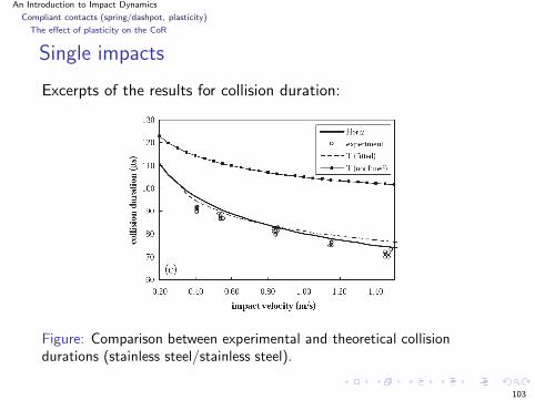
Excerpts of the results for collision duration:
Figure: Comparison between experimental and theoretical collisiondurations (stainless steel/stainless steel).
103

An Introduction to Impact Dynamics
Compliant contacts (spring/dashpot, plasticity)
The effect of plasticity on the CoR
Single impacts
Conclusions drawn in [Steven et al, Powder Techn. 2005]:
The best models are [Kuwabara and Kono, Jpn. J. Appl.Phys., 1987] and [Walton and Braun, J. Rheol., 1896] (withvariable en), both for prediction of en and collision duration.
The model of [Thorton and Ning, Powder Tech., 1998] withfitted parameter predicts well the plastic deformation effectsand collision duration, but overestimates the dependency of en
on vn(0).
104
An Introduction to Impact Dynamics
Compliant contacts (spring/dashpot, plasticity)
The effect of plasticity on the CoR
Single impacts
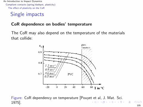
CoR dependence on bodies’ temperature
The CoR may also depend on the temperature of the materialsthat collide:
Figure: CoR dependency on temperature [Pouyet et al, J. Mat. Sci.1975].
105
An Introduction to Impact Dynamics
Compliant contacts (spring/dashpot, plasticity)
The effect of plasticity on the CoR
Single impacts
Remark: Other quantities than the CoR are worth considering:
force/identation F (δ)
energy lost during compression and during expansion
collision duration
106
An Introduction to Impact Dynamics
Compliant contacts (spring/dashpot, plasticity)
The effect of plasticity on the CoR
Single impact
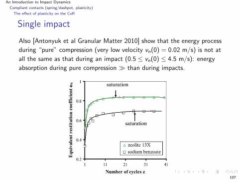
Also [Antonyuk et al Granular Matter 2010] show that the energy process
during “pure” compression (very low velocity vn(0) = 0.02 m/s) is not at
all the same as that during an impact (0.5 ≤ vn(0) ≤ 4.5 m/s): energy
absorption during pure compression ≫ than during impacts.
107
An Introduction to Impact Dynamics
Compliant contacts (spring/dashpot, plasticity)
The effect of plasticity on the CoR
Single impact
During impacts the granules lose between 15 and 27 % less energythan during pure compression, independently of:
the impact velocity (in the experimental tests range)
the maximum compression force.
However Hertz’ theory predicts well the impact process during theelastic phases.
108

An Introduction to Impact Dynamics
Compliant contacts (spring/dashpot, plasticity)
The effect of plasticity on the CoR
Single impacts
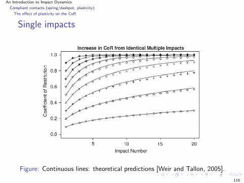
The effect of repeated impacts on plastic deformation
A recursive formula for the successive CoRs from one impact tothe next is given by [Weir and Tallon, Chem. Eng. Science, 2005] :
e83n,k+1 = e
83n,k + e
83n,1
(
1 − 2.7
(
vn,1
c0
)35
− e2n,k
)
and en,k → 1 as k → +∞: plastic deformation becomes less andless important.
[Weir and Tallon, Chem. Eng. Science, 2005] conductedexperiments of a sphere colliding an identical sphere and provedthat their analytical prediction fits well (errors ≤ 5% compared to20% with Johnson’s expression).
109
An Introduction to Impact Dynamics
Compliant contacts (spring/dashpot, plasticity)
The effect of plasticity on the CoR
Single impacts
Figure: Continuous lines: theoretical predictions [Weir and Tallon, 2005].
110
An Introduction to Impact Dynamics
Compliant contacts (spring/dashpot, plasticity)
The effect of plasticity on the CoR
Single impacts
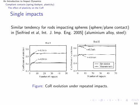
Similar tendency for rods impacting spheres (sphere/plane contact)in [Seifried et al, Int. J. Imp. Eng. 2005] (aluminium alloy, steel):
Figure: CoR evolution under repeated impacts.
111
An Introduction to Impact Dynamics
Compliant contacts (spring/dashpot, plasticity)
Wave effects and the validity of the quasistatic assumption
Single impacts
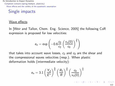
Wave effects
In [Weir and Tallon, Chem. Eng. Science, 2005] the following CoRexpression is proposed for low velocities:
en = exp
(
−0.6c0
c2
(
vn(0)
c0
)35
)
that takes into account wave losses, c2 and c0 are the shear andthe compressional waves velocities (resp.). When plasticdeformation holds (intermediate velocity):
en = 3.1
(
Yd
E ∗
) 58(
R1
R
) 38(
c0
vn(0)
) 14
112
An Introduction to Impact Dynamics
Compliant contacts (spring/dashpot, plasticity)
Wave effects and the validity of the quasistatic assumption
Single impacts
It seems from the above that even in the case of two spherescolliding, some wave effects may be important for an accurateprediction of the impact outcome.
Many experimental and analytical studies have proved thateven for perfectly elastic materials the wave effects may besignificant (up to 5% energy loss). Therefore the quasistaticassumption may not be suitable.
We’ll see later in these lectures that waves also play asignificant role in multiple impacts, but for a different reason(dispersion of energy rather than dissipation of energy).
113
An Introduction to Impact Dynamics
Compliant contacts (spring/dashpot, plasticity)
Conclusions
Single impacts
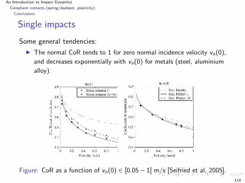
Some general tendencies:
The normal CoR tends to 1 for zero normal incidence velocity vn(0),
and decreases exponentially with vn(0) for metals (steel, aluminium
alloy).
Figure: CoR as a function of vn(0) ∈ [0.05− 1] m/s [Seifried et al, 2005].
114
An Introduction to Impact Dynamics
Compliant contacts (spring/dashpot, plasticity)
Conclusions
Single impacts
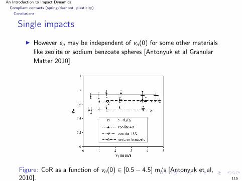
However en may be independent of vn(0) for some other materials
like zeolite or sodium benzoate spheres [Antonyuk et al Granular
Matter 2010].
Figure: CoR as a function of vn(0) ∈ [0.5 − 4.5] m/s [Antonyuk et al,2010]. 115
An Introduction to Impact Dynamics
Compliant contacts (spring/dashpot, plasticity)
Conclusions
Single impacts
Plastic dissipation effects play a role only during the firstimpacts, so that usually en increases with the number ofimpacts (not always true however, for some materialssoftening, microcracking and breakage produce the reversephenomenon [Tavares et al, Powder Tech. 2002]).
Elastic waves may dissipate energy even in elastic bodies thatimpact, and call into question quasistatic assumptions (evenfor very simple geometries like disks impacting an anvil).
116

An Introduction to Impact Dynamics
General conclusions on single impact models
Single impacts
Many theoretical and experimental studies that concern:
(a) macroscopic coefficients and algebraic impact laws
(b) detailed studies on the normal restitution coefficient andits dependence on mechanical parameters (local effects) forsphere/plane, starting from Hertz’ theory.
(c) incorporation of wave effects (global effects)
Which conclusions may be drawn from all these works? Can wededuce some general guidelines?
117
An Introduction to Impact Dynamics
General conclusions on single impact models
Single impacts
The impact with friction phenomenon is extremely complex andinvolves (too) many physical phenomena. Two general directionsmay be drawn:
If the impact is very simple (colinear, sphere/sphere orsphere/plane), may use a refined complex expression of therestitution coefficient if needed.
If the impact is complex, better use constant coefficients andalgebraic law (at the price of fitting, may be). Then you maywant the law to provide a unique and admissible solution forany initial data, and be numerically tractable.
In any case if a fine model is needed then it has to be tayloredto the application.
Next we shall deal with multiple impacts!
118
An Introduction to Impact Dynamics
General conclusions on single impact models
Single impacts
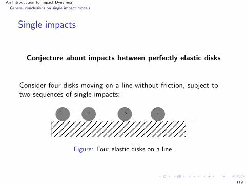
Conjecture about impacts between perfectly elastic disks
Consider four disks moving on a line without friction, subject totwo sequences of single impacts:
2 41 3
Figure: Four elastic disks on a line.
119
An Introduction to Impact Dynamics
General conclusions on single impact models
Single impacts
Initially no vibrations inside the bodies. Scenario:
Initial velocities and initial kinetic energy (∑4
i=112miv
2Gi
(0))
impact between 1 and 2, and between 3 and 4
the bodies are excited by vibrations transmitted by the impactso that en < 1 at both contacts
1 and 4 leave
2 and 3 collide again and transfer all their pre-imact energy(kinetic energy of the mass enter + vibrational energy) intomass centers velocities so that en > 1.
The final kinetic energy is equal to the initial one and is∑4
i=112miv
2Gi
(0)
120
An Introduction to Impact Dynamics
General conclusions on single impact models
Multiple impacts
Let us now pass to the problem of multiple impact modeling.
121
An Introduction to Impact Dynamics
Definitions
The gap functions
Multiple impacts
Let q ∈ Rn denote the vector of independent generalized
coordinates of the system in a free-motion mode (i.e. the contactpoints of interest are supposed to be inactive). The inertia matrixis denoted as M(q) assumed to be symmetric positive definite.
The gap functions hi (q) ≥ 0, 1 ≤ i ≤ m, are used to state thenon-penetrability of the contacting bodies. They are signeddistances.
We define the m gap functions hi : Rn → R as differentiable
functions.In general they are hard to compute analytically, so a numerical
estimation is necessary (collision detection algorithms).
122
An Introduction to Impact Dynamics
Definitions
The gap functions
Multiple impacts
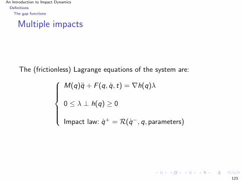
The (frictionless) Lagrange equations of the system are:
M(q)q + F (q, q, t) = ∇h(q)λ
0 ≤ λ ⊥ h(q) ≥ 0
Impact law: q+ = R(q−, q, parameters)
123
An Introduction to Impact Dynamics
Definitions
A multiple impact in a multibody system
Multiple impacts
DefinitionLet Φ = q ∈ R
n | h(q) ≥ 0 be the admissible domain of themechanical system. A multiple impact of order p (or a p−impact)is an impact that occurs at a codimension p singularity of theboundary bd(Φ).
124
An Introduction to Impact Dynamics
Definitions
A multiple impact in a multibody system
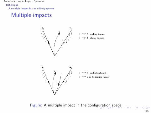
Multiple impacts
Figure: A multiple impact in the configuration space
125
An Introduction to Impact Dynamics
Definitions
The kinetic angle between two hypersurfaces
Multiple impacts
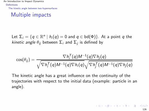
Let Σi = q ∈ Rn | hi(q) = 0 and q ∈ bd(Φ). At a point q the
kinetic angle θij between Σi and Σj is defined by
cos(θij) =∇hT
i (q)M−1(q)∇hj(q)√
∇hTi (q)M−1(q)∇hi (q)
√
∇hTj (q)M−1(q)∇hj(q)
The kinetic angle has a great influence on the continuity of thetrajectories with respect to the initial data (example: particle in anangle).
126
An Introduction to Impact Dynamics
Definitions
The kinetic angle between two hypersurfaces
Multiple impacts
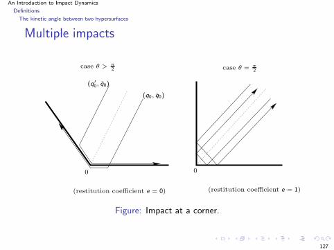
(q′
0, q0)
case θ > π2 case θ = π
2
0 0
(q0, q0)
(restitution coefficient e = 0) (restitution coefficient e = 1)
Figure: Impact at a corner.
127

An Introduction to Impact Dynamics
Definitions
The kinetic angle between two hypersurfaces
Multiple impacts
A result of [Paoli, 2005] states that continuity with respect toinitial data holds under certain conditions, roughly:
〈∇hi (q),M−1(q)∇hj(q)〉 ≤ 0 if en = 0 (19)
(0 ≤ θij ≤ π2 )
〈∇hi (q),M−1(q)∇hj(q)〉 = 0 if en ∈ (0, 1] (20)
(θij = π2 )
hold for all indices i , j ∈ I (q), i 6= j .
128

An Introduction to Impact Dynamics
Definitions
The kinetic angle between two hypersurfaces
Multiple impacts
Remark: what does this become when one considers constraintswith Coulomb’s friction ?
Indeed the presence of dry friction usually destroys the nicefrictionless orthogonality properties (due to the fact that euclideanand kinetic metrics do not match).
129
An Introduction to Impact Dynamics
Definitions
Examples
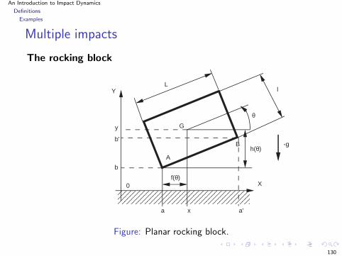
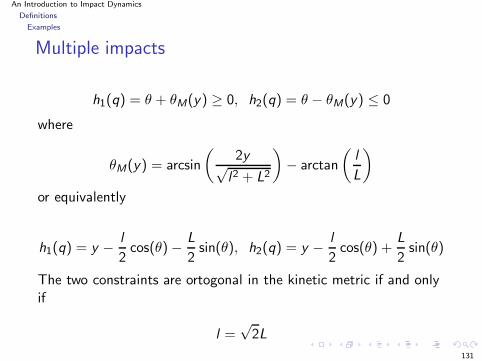
Multiple impacts
The rocking block
AAAAAAAAAAAAAAAAAAAAAAAAAAAAAAAAAAAA
G
Ll
B
A
b'
y
b
a x a'
X
Y
θ
h(θ)
f(θ)0
-g
Figure: Planar rocking block.
130
An Introduction to Impact Dynamics
Definitions
Examples
Multiple impacts
h1(q) = θ + θM(y) ≥ 0, h2(q) = θ − θM(y) ≤ 0
where
θM(y) = arcsin
(
2y√l2 + L2
)
− arctan
(
l
L
)
or equivalently
h1(q) = y − l
2cos(θ) − L
2sin(θ), h2(q) = y − l
2cos(θ) +
L
2sin(θ)
The two constraints are ortogonal in the kinetic metric if and onlyif
l =√
2L
131
An Introduction to Impact Dynamics
Definitions
Examples
Multiple impacts
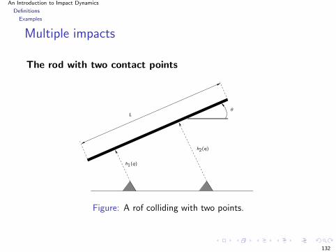
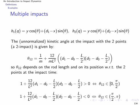
The rod with two contact points
h1(q)
h2(q)
Lθ
Figure: A rof colliding with two points.
132

An Introduction to Impact Dynamics
Definitions
Examples
Multiple impacts
The rod at the impact:
d0
d1
d2
L
Figure: A rof colliding with two points.
133
An Introduction to Impact Dynamics
Definitions
Examples
Multiple impacts
h1(q) = y cos(θ)+(d1−x) sin(θ), h2(q) = y cos(θ)+(d2−x) sin(θ)
The (unnormalized) kinetic angle at the impact with the 2 points(a 2-impact) is given by:
θ12 =1
m+
12
mL2
(
(d1 − d0 −L
2)(d2 − d0 −
L
2)
)
so θ12 depends on the rod length and on its position w.r.t. the 2points at the impact time:
1 +12
L2(d1 − d0 −
L
2)(d2 − d0 −
L
2) > 0 ⇔ θ12 ∈ [0,
π
2)
1 +12
L2(d1 − d0 −
L
2)(d2 − d0 −
L
2) < 0 ⇔ θ12 ∈ (
π
2, π)
134

An Introduction to Impact Dynamics
Definitions
Examples
Multiple impacts
The analysis indicates that some configurations may be yield quite“stable” impacts, while some others yield impact outcomes quitesensitive to initial data.
135
An Introduction to Impact Dynamics
The lagrangian impact dynamics
Multiple impacts
At a time t when a shock occurs, λ is a Dirac measure and so isthe acceleration q. Positions q remain constant and velocities qundergo a discontinuity.
M(q(t))[q(t+) − q(t−)] = ∇h(q(t))pt
where λ = ptδt , pt being the percussion at time t.
There are n + m unknowns: q(t+) and pt . We have n equations,so we need m more equations just to solve the problem.
136
An Introduction to Impact Dynamics
The lagrangian impact dynamics
A state vector change
Multiple impacts
Let us now transform the Lagrange impact dynamics using somespecific state vetcor change.
The unitary normal vector to each hypersurface of constrainthi (q) = 0, 1 ≤ i ≤ m, in the kinetic metric is
nq,i =M−1(q)∇hi (q)
√
∇hTi (q)M−1(q)∇hi (q)
Unitary tangent vectors are defined as
tTq,j∇hi(q) = 0
for all 1 ≤ i ≤ m. So we have constructed an orthonormal frame inthe configuration space, at q. We collect all nq,i into nq ∈ R
m andall tq,j into tq ∈ R
n−m.
137
An Introduction to Impact Dynamics
The lagrangian impact dynamics
A state vector change
Multiple impacts
Let’s perform a specific state vector change as follows: Let
Ξ =
(
nTq
tTq
)
and letM(q) = ΞM(q)
The new vector of velocities is:
(
qnorm
qtan
)
= M(q)q
that splits the generalized velocity into a “normal” and a“tangential” components (in the kinetic metric).
138
An Introduction to Impact Dynamics
The lagrangian impact dynamics
A state vector change
Multiple impacts
Then the Lagrange dynamics is transformed into:
qnorm + F1(q, q, t) = nqFq
qtan + F2(q, q, t) = 0(21)
because the constraints are frictionless. At an impact time one hasFq = pqδt . The term pq = ∇h(q)p ∈ R
n is the generalizedpercussion vector, p ∈ R
m.
At an impact time t we get:
qnorm(t+) − qnorm(t−) = nqpq
and
qtan(t+) = qtan(t
−)
139

An Introduction to Impact Dynamics
The lagrangian impact dynamics
A state vector change
This transformation may make us think that the generalisedproblem in configuration space is equivalent to the simple particlecase...
But this is not true!
One example of the limitations of the Lagrange formalism (gain formathematicians, not for mechanicians...)
140
An Introduction to Impact Dynamics
The lagrangian impact dynamics
A state vector change
Multiple impacts
The pairwise orthogonality of the constraints is stated in the newdynamics as:
nTq,iM(q)nq,j = ∇hT
i (q)M−1(q)∇hj(q) = 0
which corresponds to the Delassus’ matrix being diagonal and theimpact dynamics being decoupled (the impact on Σi does notinfluence the impacts on Σj for all j 6= i).
(The Delassus’ matrix is ∇hT (q)M−1(q)∇h(q) ∈ Rm×m.)
141
An Introduction to Impact Dynamics
The lagrangian impact dynamics
A state vector change
Multiple impacts
One may write a generalized frictionless impact law as follows foreach constraint hi (q). 1 ≤ i ≤ m:
q+norm,i = −en,i q−
norm,i (22)
that yields if all constraints are impacted simultaneously:
TL =1
2
m∑
i=1
(e2n,i − 1)(q−
norm,i )2 (23)
Let m = 1 (one contact), or let en,i = en for all i . Then TL ≤ 0implies |en| ≤ 1 similarly to the frictionless two-particle case.
142
An Introduction to Impact Dynamics
The lagrangian impact dynamics
A state vector change
Multiple impacts
Remark
Applying the normal restitution in (22) is equivalent toapplying Moreau’s rule.
There is no generalized formulation of Coulomb’s frictionusing directly the qtan components.
Clearly we may also define some generalized “tangential”restitution coefficients et,i , 1 ≤ i ≤ n − m and construct a“generalized restitution mapping”. However will this be quiteuseful if such a restitution mapping does not satisfy most ofthe requirements for a good impact law (see few slides below)?
143
An Introduction to Impact Dynamics
The lagrangian impact dynamics
A state vector change
Multiple impacts
Rocking block example
Considering only the left contact point one has:
qnorm,1 =qT∇qf1(q)
√
∇qf1(q)TM−1(q)∇qf1(q)
with qT∇qf1(q) = 2√l2+L2−4y2
y + θ, and
qtang,1 =
( √mx
m√4I+mL2
y(t−k ) − 2IL√
4I+mL2θ(t−k )
)
(24)
144
An Introduction to Impact Dynamics
The lagrangian impact dynamics
A state vector change
Multiple impacts
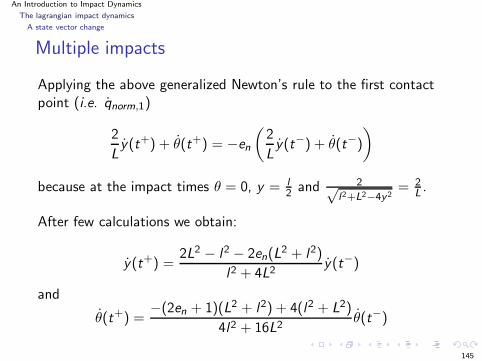
Applying the above generalized Newton’s rule to the first contactpoint (i.e. qnorm,1)
2
Ly(t+) + θ(t+) = −en
(
2
Ly(t−) + θ(t−)
)
because at the impact times θ = 0, y = l2 and 2√
l2+L2−4y2= 2
L.
After few calculations we obtain:
y(t+) =2L2 − l2 − 2en(L
2 + l2)
l2 + 4L2y(t−)
and
θ(t+) =−(2en + 1)(L2 + l2) + 4(l2 + L2)
4l2 + 16L2θ(t−)
145
An Introduction to Impact Dynamics
The lagrangian impact dynamics
A state vector change
Multiple impacts
This is to be compared with the widely used Housner’s model thattreats the rocking block as a one degree-of-freedom system andstates that
θ(t+) = −e θ(t−)
This tends to indicate that such a e depends on the blockdimensions and on en.
two “normal” generalised restitution coefficients certainly notenough to describe rocking motion (already noticed by Moreau).
We’ll introduce later a matrix of generalised restitution coefficients.
146
An Introduction to Impact Dynamics
The lagrangian impact dynamics
First conclusions
Multiple impacts
The impact dynamics may be stated in the configuration space.This allows us to point out two important features:
The kinetic angle between the constraints plays a role in thetrajectories properties
The fact that contacts are of a local nature may complicatethe analysis because the local orthogonality (euclidean) doesnot transport to generalized (“global”) orthogonality (kinetic).
The three-ball chain will serve as an illustration.
147
An Introduction to Impact Dynamics
Features and properties of a restitution mapping
Multiple impacts
(1) the kinetic angle between the surfaces Σi , 1 ≤ i ≤ pinvolved in the p−impact,
(2) the (dis)continuity of the solutions with respect to theinitial data,
(3) the kinetic energy behavior at the impact,
(4) the wave effects due to the coupling between variouscontacts,
(5) the local energy loss during impacts,
(6) the ability of the impact rule to span the whole admissiblepost-impact velocities domain,
(7) the ability of the parameters defining the impact rule tobe identified from experiments,
148
An Introduction to Impact Dynamics
Features and properties of a restitution mapping
Multiple impacts
(8) the (in)dependence of these parameters on the initial data,
(9) the physical meaning of the parameters of the impact rule,
(10) the ability of the impact rule to provide post-impactvelocities in agreement with experimental results,
(11) the well-posedness of the nonsmooth dynamics when theimpact rule is incorporated in it,
(12) the law should be applicable (or easily extendable) togeneral mechanical systems,
(13) the determination of the impact termination,
(14) the impact law has to be numerically tractable.
149
An Introduction to Impact Dynamics
Features and properties of a restitution mapping
Some items are peculiar to multiple shocks, like item (4) aboutwave effects: waves through the bodies are responsible for thedispersion of the energy.
Energy dispersion
This characterizes the fact that the kinetic energy is distributedamong the bodies of the system during the shock, as a result ofwaves effects that travel throughout the mechanical system.
150

An Introduction to Impact Dynamics
Simple chains of balls (3-ball, 2-ball and wall)
Multiple impacts
Let’s focus on chains of balls.
Why study chains of balls ?
Chains of balls are a widely studied system with multipleimpacts: looks simple, but is not at all!
May be seen as the simplest granular material.
151
An Introduction to Impact Dynamics
Simple chains of balls (3-ball, 2-ball and wall)
Textbooks solutions and experimental results
Multiple impacts
The “textbooks solution” concerns solely the case of one ball thatimpacts a chain of balls at rest and in contact. Then q+
n = q−1 ,
while q+i = 0 for all 1 ≤ i ≤ n − 1, i.e. all the energy is transferred
from the first to the last ball.
This is however contradicted by most experiments where it isapparent that q+
i 6= 0 for all 1 ≤ i ≤ n − 1!
effects of the dispersion of the kinetic energy in the chain, dueto waves that travel throughout the chain (this is a mechanicaltsunami).
152
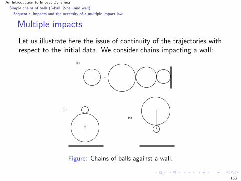
An Introduction to Impact Dynamics
Simple chains of balls (3-ball, 2-ball and wall)
Sequential impacts and the necessity of a multiple impact law
Multiple impacts
Let us illustrate here the issue of continuity of the trajectories withrespect to the initial data. We consider chains impacting a wall:
(c)
(b)
(a)
Figure: Chains of balls against a wall.
153
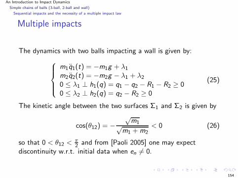
An Introduction to Impact Dynamics
Simple chains of balls (3-ball, 2-ball and wall)
Sequential impacts and the necessity of a multiple impact law
Multiple impacts
The dynamics with two balls impacting a wall is given by:
m1q1(t) = −m1g + λ1
m2q2(t) = −m2g − λ1 + λ2
0 ≤ λ1 ⊥ h1(q) = q1 − q2 − R1 − R2 ≥ 00 ≤ λ2 ⊥ h2(q) = q2 − R2 ≥ 0
(25)
The kinetic angle between the two surfaces Σ1 and Σ2 is given by
cos(θ12) = −√
m1√m1 + m2
< 0 (26)
so that 0 < θ12 < π2 and from [Paoli 2005] one may expect
discontinuity w.r.t. initial data when en 6= 0.
154
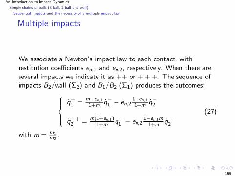
An Introduction to Impact Dynamics
Simple chains of balls (3-ball, 2-ball and wall)
Sequential impacts and the necessity of a multiple impact law
Multiple impacts
We associate a Newton’s impact law to each contact, withrestitution coefficients en,1 and en,2, respectively. When there areseveral impacts we indicate it as ++ or + + +. The sequence ofimpacts B2/wall (Σ2) and B1/B2 (Σ1) produces the outcomes:
q+1 =
m−en,1
1+mq−1 − en,2
1+en,1
1+mq−2
q++2 =
m(1+en,1)1+m
q−1 − en,2
1−en,1m
1+mq−2
(27)
with m = m1m2
.
155
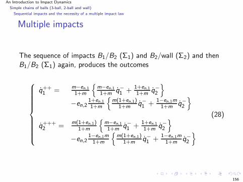
An Introduction to Impact Dynamics
Simple chains of balls (3-ball, 2-ball and wall)
Sequential impacts and the necessity of a multiple impact law
Multiple impacts
The sequence of impacts B1/B2 (Σ1) and B2/wall (Σ2) and thenB1/B2 (Σ1) again, produces the outcomes
q++1 =
m−en,1
1+m
m−en,1
1+mq−1 +
1+en,1
1+mq−2
−en,21+en,1
1+m
m(1+en,1)1+m
q−1 +
1−en,1m
1+mq−2
q+++2 =
m(1+en,1)1+m
m−en,1
1+mq−1 +
1+en,1
1+mq−2
−en,21−en,1m
1+m
m(1+en,1)1+m
q−1 +
1−en,1m
1+mq−2
(28)
156
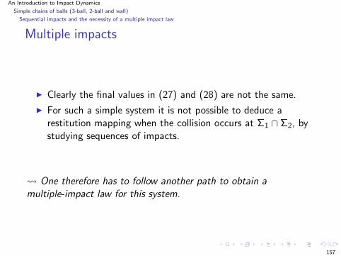
An Introduction to Impact Dynamics
Simple chains of balls (3-ball, 2-ball and wall)
Sequential impacts and the necessity of a multiple impact law
Multiple impacts
Clearly the final values in (27) and (28) are not the same.
For such a simple system it is not possible to deduce arestitution mapping when the collision occurs at Σ1 ∩ Σ2, bystudying sequences of impacts.
One therefore has to follow another path to obtain amultiple-impact law for this system.
157
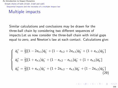
An Introduction to Impact Dynamics
Simple chains of balls (3-ball, 2-ball and wall)
Sequential impacts and the necessity of a multiple impact law
Multiple impacts
Similar calculations and conclusions may be drawn for thethree-ball chain by considering two different sequences ofimpacts.Let us now consider the three-ball chain with initial gapsequal to zero, and Newton’s law at each contact. Calculations give:
q+1 = 1
3 [(1 − 2en,1)q−1 + (1 − en,2 + 2en,1)q
−2 + (1 + en,2)q
−3 ]
q+2 = 1
3 [(1 + en,1)q−1 + (1 − en,2 − en,1)q
−2 + (1 + en,2)q
−3 ]
q+3 = 1
3 [(1 + en,1)q−1 + (1 + 2en,2 − en,1)q
−2 + (1 − 2en,2)q
−3 ](29)
158
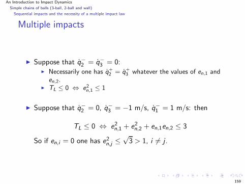
An Introduction to Impact Dynamics
Simple chains of balls (3-ball, 2-ball and wall)
Sequential impacts and the necessity of a multiple impact law
Multiple impacts
Suppose that q−2 = q−
3 = 0: Necessarily one has q+
2 = q+3 whatever the values of en,1 and
en,2. TL ≤ 0 ⇔ e2
n,1 ≤ 1
Suppose that q−2 = 0, q−
3 = −1 m/s, q−1 = 1 m/s: then
TL ≤ 0 ⇔ e2n,1 + e2
n,2 + en,1en,2 ≤ 3
So if en,i = 0 one has e2n,j ≤
√3 > 1, i 6= j .
159
An Introduction to Impact Dynamics
Simple chains of balls (3-ball, 2-ball and wall)
Sequential impacts and the necessity of a multiple impact law
Notice that this is equivalent to applying Moreau’s law formulatedin the generalized coordinates. In particular if en = 0 in Moreau’slaw then
q+1 = q+
2 = q+3 =
1
3(q−
1 + q−2 + q−
3 )
the three balls are stuck together after the impact.
Notice: maximum dissipation does not mean that the three ballscome to rest after the impact...
160
An Introduction to Impact Dynamics
Simple chains of balls (3-ball, 2-ball and wall)
First conclusions
Multiple impacts
It is inferred from this simple example that the kineticcoefficients (associated to pairs of balls) are unable to modelneither the dissipation nor the dispersion effects.
The upper bounds of the coefficients vary with the initial data!
There is not a unique choice for en,1 and en,2 even for a givenenergetical behaviour: TL = 0 means e2
n,1 + e2n,2 + en,1en,2 = 3
in the second case.
Let’s examine now what happens when some compliance is addedbetween the balls.
161
An Introduction to Impact Dynamics
Simple chains of balls (3-ball, 2-ball and wall)
Compliant contacts (lumped flexibilities)
Multiple impacts
Let us illustrate on a linear chain with linear or Hertz unilateralsprings the fact that under a constant energetical behaviour (hereno energy loss) the impact outcome may vary a lot with thestiffness ratio γ and the initial velocities.
162
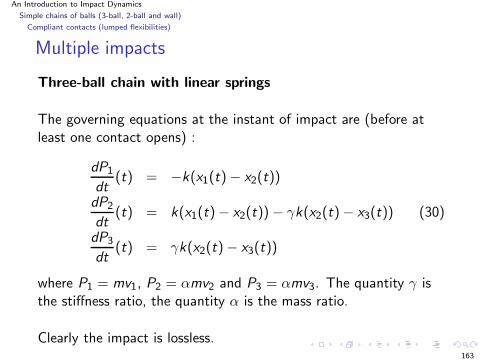
An Introduction to Impact Dynamics
Simple chains of balls (3-ball, 2-ball and wall)
Compliant contacts (lumped flexibilities)
Multiple impacts
Three-ball chain with linear springs
The governing equations at the instant of impact are (before atleast one contact opens) :
dP1
dt(t) = −k(x1(t) − x2(t))
dP2
dt(t) = k(x1(t) − x2(t)) − γk(x2(t) − x3(t)) (30)
dP3
dt(t) = γk(x2(t) − x3(t))
where P1 = mv1, P2 = αmv2 and P3 = αmv3. The quantity γ isthe stiffness ratio, the quantity α is the mass ratio.
Clearly the impact is lossless.163
An Introduction to Impact Dynamics
Simple chains of balls (3-ball, 2-ball and wall)
Compliant contacts (lumped flexibilities)
Multiple impacts
It is possible to show (analytically) that:
If γ → +∞ then q+1 = −1
3 m/s q+2 = q+
3 = 23 m/s
If γ → 0 then limγ→0 q+1 = 0 m/s, limγ→0 q+
2 = 0 m/s,limγ→0 q+
3 = 1 m/s.
one retrieves two “familiar” outcomes.
Several detailed studies of such chains have been published in theAmerican J. of Physics. For instance [Reinsch, Am. J. Phys. 1994]shows that the “dispersion-free” outcome (the second one) canappear for an infinity of suitable γ and α in n−ball chains.
164
An Introduction to Impact Dynamics
Simple chains of balls (3-ball, 2-ball and wall)
Compliant contacts (lumped flexibilities)
Multiple impacts
One may however question the usefulness of such conclusionsdrawn for linear elastic contacts, since the right stiffness for chainsof balls is Hertz nonlinear stiffness [Falcon et al, 1998].
It is not clear whether or not linear springs may well model waveeffects through the chain, because Hertz contact bringsnonlinearity which makes waves behave differently (even in thecase of pre-compression in the chain).
165
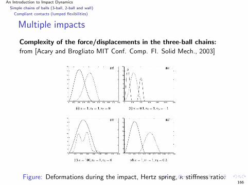
An Introduction to Impact Dynamics
Simple chains of balls (3-ball, 2-ball and wall)
Compliant contacts (lumped flexibilities)
Multiple impacts
Complexity of the force/displacements in the three-ball chains:
from [Acary and Brogliato MIT Conf. Comp. Fl. Solid Mech., 2003]
Figure: Deformations during the impact, Hertz spring, κ stiffness ratio.166
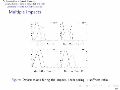
An Introduction to Impact Dynamics
Simple chains of balls (3-ball, 2-ball and wall)
Compliant contacts (lumped flexibilities)
Multiple impacts
Figure: Deformations furing the impact, linear spring, κ stiffness ratio.
167
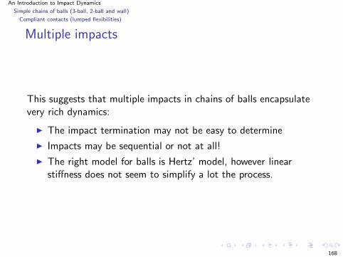
An Introduction to Impact Dynamics
Simple chains of balls (3-ball, 2-ball and wall)
Compliant contacts (lumped flexibilities)
Multiple impacts
This suggests that multiple impacts in chains of balls encapsulatevery rich dynamics:
The impact termination may not be easy to determine
Impacts may be sequential or not at all!
The right model for balls is Hertz’ model, however linearstiffness does not seem to simplify a lot the process.
168
An Introduction to Impact Dynamics
Simple chains of balls (3-ball, 2-ball and wall)
Further analysis of n−ball chains
Multiple impacts
[Reinsch 1994, Am. J. Phys.] computes masses and stiffnesses ratios sothat a linear chain is dispersion-free, which means that if n left-ballsimpact m right-balls at rest, then n right-balls leave the chain while mleft-balls stay at rest after the shock.
This is however very sensitive with respect to the parameters.
Some contacts may last very long under some configurations andinitial data.
Waves depend a lot on whether this is linear of nonlinear (Hertz orelse) elasticity, independently of pre-loading or not (the nonlinearmodes play an important role). So the validity of studies based onlinear elastic contact may be questioned for chains of balls.
Notice however that [Bayman, 1976] shows that chains of elasticrods are dispersion-free.
And what about the effect of dissipation on the dispersion (wavedissipation due to the viscoelastic property of the material) ?
169
An Introduction to Impact Dynamics
First conclusions
Multiple impacts
Sequential impacts analysis based on pair-wise collisions onsimple multibody systems show that excepted some extremelyparticular cases, this is a hopeless path to get a multipleimpact law because there is not a unique limit as the gapstend to zero (kinetic angle 6= π
2 ). Compliant contact models show that the multiple impact
process may be extremely complex and may display a varietyof behaviours (dispersion, dispersion-free, short contact, longlasting contacts), even if the kinetic energy loss is fixed.
How to represent wave effects (dispersion of kinetic energy)with constant parameters within a perfect rigid bodyframework and algebraic impact dynamics ?? (in particularsatisfying item (8) above).
Personal conjecture: this is impossible...
170
An Introduction to Impact Dynamics
Multiple impact restitution mappings
A generalized Newton’s law
Multiple impacts
One may start from a quite general point of view and derive ageneral restitution mapping for generalized velocities using forinstance the above (qnorm, qtan):
(
q+norm
q+tan
)
= E(
q−norm
q−tan
)
(31)
Drawback: no clear physical meaning of the coefficients, adaptthe coefficients values to each system configuration (see items (4)(7) (8) (9) above).
171
An Introduction to Impact Dynamics
Multiple impact restitution mappings
A generalized Newton’s law
Multiple impacts
Consider for instance the rocking block:
Rocking motion implies that en,1 = en,2 = 0 (the contactsstick after the impacts).
Now for other configurations one needs en,i 6= 0 to allow forrebound.
So the mechanical meaning of such coefficients is not clear.They may have to be changed depending on the initial data.
172

An Introduction to Impact Dynamics
Multiple impact restitution mappings
A generalized Newton’s law
Multiple impacts
Other impact mappings:
Fremond (use of Moreau’s superpotential; coefficients may bemeaningless depending on the superpotential choice)
Pfeiffer and Glocker (use two LCPs and a Poisson-likecoefficient; energetical behaviour not always guaranteed)
Ceanga and Hurmuzlu (Routh’s method, e∗,i , and impulsecorrelation ratio – unfortunately dependent on system’s data,numerical implementation not obvious)
173

An Introduction to Impact Dynamics
Multiple impact restitution mappings
Extension of the Darboux-Keller’s approach
Multiple impacts
Let’s describe now a recent approach that seems to provide goodresults on chains of balls and bouncing dimers.
We first deal with frictionless multiple impacts.
174
An Introduction to Impact Dynamics
Multiple impact restitution mappings
Extension of the Darboux-Keller’s approach
Multiple impacts
Darboux-Keller approach is extended to the case of multipleimpacts:
rate independent materials
bilinear stiffness model to represent non reversible loss ofenergy effects like plastic deformation
possibility to vary the elasticity coefficient (linear, Hertz, orelse)
allow for several compression/expansion cycles at eachcontact point
energetic coefficients of restitution at each contact point withe∗,i ∈ [0, 1]
numerical results match well with several experimental results
175
An Introduction to Impact Dynamics
Multiple impact restitution mappings
Extension of the Darboux-Keller’s approach
Multiple impacts
Starting from the Lagrange equations and proceeding for instanceas Pfeiffer and Glocker (1995,1996) we may obtain the shockdynamics as:
Mdq − WdP = 0
The mass matrix M and the jacobian matrix W remain unchangedduring the impact by assumption. The relative velocity of thecontact points is expressed as
δi (q, t) = wTi (q, t)q + wi(q, t)
The matrix W collects the terms wi , and dP is the vector ofnormal impulses.
176
An Introduction to Impact Dynamics
Multiple impact restitution mappings
Extension of the Darboux-Keller’s approach
Multiple impacts
We suppose that the force/indentation mapping at the contactpoint i is:
λi = Ki (δi )η (32)
where Ki is the contact stiffness, the exponent η determines thekind of contacts between bodies (η = 3
2 is for Hertz contact, η = 1is linear elasticity).
Let Pi (t) denote the total normal impulse accumulated during thetime interval [0, t]: Pi(t) = Pi(0) +
∫ t
0 λi(s)ds. So dPi
dt(t) = λi (t)
and:dλi
dt=
dλi
dPi· dPi
dt= λi
dλi
dPi(33)
177
An Introduction to Impact Dynamics
Multiple impact restitution mappings
Extension of the Darboux-Keller’s approach
Multiple impacts
In terms of the compliant model expressed by (32), we have
dλi
dt= ηKi (δi )
η−1δi = ηKi (δi )η−1wT
i q (34)
Notice that δi can always be expressed as
δi =
(
λi
Ki
)1η
(35)
Substituting (35) and (34) into (33) leads to
λi
1η dλi = ηKi
1η wT
i qdPi (36)
178
An Introduction to Impact Dynamics
Multiple impact restitution mappings
Extension of the Darboux-Keller’s approach
Multiple impacts
The initial value of the normal impulse can be set to Pi (0) = 0,and the contact force before impact is λi(0) = 0 for the casewithout initial precompression energy.
The integration of equation (36) leads to
λi(Pi (t)) =
[
(η + 1)
∫ Pi (t)
0Ki
1η wT
i qdPi
]η
η+1
(37)
179
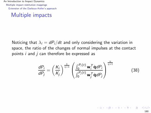
An Introduction to Impact Dynamics
Multiple impact restitution mappings
Extension of the Darboux-Keller’s approach
Multiple impacts
Noticing that λi = dPi/dt and only considering the variation inspace, the ratio of the changes of normal impulses at the contactpoints i and j can therefore be expressed as
dPi
dPj=
(
Ki
Kj
)1
η+1
∫ Pi (t)0 wT
i qdPi∫ Pj (t)0 wT
j qdPj
η
η+1
(38)
180

An Introduction to Impact Dynamics
Multiple impact restitution mappings
Extension of the Darboux-Keller’s approach
Multiple impacts
The work functions at both contact points are defined as:
Ei =
∫ Pi (t)
0wT
i qdPi , Ej =
∫ Pj (t)
0wT
j qdPj (39)
Ei and Ej are the works of the normal contact forces at contactpoints i and j from the beginning of impacts to the instant Pi
(resp. Pj ), in which the energy is mapped into the velocity-impulselevel.
These terms can also be thought of as the potential energy storedin the springs at contact points i and j .
181
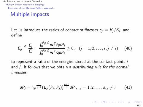
An Introduction to Impact Dynamics
Multiple impact restitution mappings
Extension of the Darboux-Keller’s approach
Multiple impacts
Let us introduce the ratios of contact stiffnesses γji = Kj/Ki , anddefine
Eji∆=
Ej
Ei=
∫ Pj (t)0 wT
j qdPj∫ Pi (t)0 wT
i qdPi
≥ 0, (j = 1, 2, . . . , s, j 6= i) (40)
to represent a ratio of the energies stored at the contact points iand j . It follows that we obtain a distributing rule for the normalimpulses:
dPj = γji
1η+1 (Eji (Pi ,Pj))
η+1η dPi , j = 1, 2, . . . , s, j 6= i (41)
182

An Introduction to Impact Dynamics
Multiple impact restitution mappings
Extension of the Darboux-Keller’s approach
Multiple impacts
These expressions reflect the wave behaviors generated inmultiple impacts and depend only on the properties of thecontact constraints: the relative stiffness and the relativepotential energies accumulated in the contact points.
Since the potential energy at contact points will changeduring impacts, the assumption that the distribution ofnormal impulses are constant (as stated in [Ceanga andHurmuzlu, JAM 2001] by defining a constant ICR) is invalidin most cases. Confirmed by [Acary and Brogliato, 2003] fromcalculations of ICRs with Hertz elasticity.
As indicated e.g. in [Falcon et al, Eur. J. Phys. 1998] and[Luding et al, Phys. Rev. E, 1994], the wave effects are dueto the elastic properties of the bodies (though it seems thatthe local dissipations at the contacts may influence them).
183
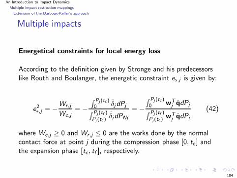
An Introduction to Impact Dynamics
Multiple impact restitution mappings
Extension of the Darboux-Keller’s approach
Multiple impacts
Energetical constraints for local energy loss
According to the definition given by Stronge and his predecessorslike Routh and Boulanger, the energetic constraint es,j is given by:
e2∗,j = −Wr ,j
Wc,j= −
∫ Pj (tc )0 δjdPj∫ Pj (tf )
Pj (tc )δjdPNj
= −∫ Pj (tc )0 wT
j qdPj
∫ Pj (tf )
Pj (tc )wT
j qdPj
(42)
where Wc,j ≥ 0 and Wr ,j ≤ 0 are the works done by the normalcontact force at point j during the compression phase [0, tc ] andthe expansion phase [tc , tf ], respectively.
184
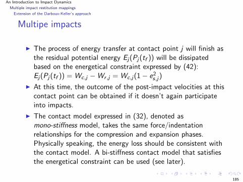
An Introduction to Impact Dynamics
Multiple impact restitution mappings
Extension of the Darboux-Keller’s approach
Multipe impacts
The process of energy transfer at contact point j will finish asthe residual potential energy Ej(Pj (tf )) will be dissipatedbased on the energetical constraint expressed by (42):Ej(Pj (tf )) = Wc,j − Wr ,j = Wc,j(1 − e2
s,j)
At this time, the outcome of the post-impact velocities at thiscontact point can be obtained if it doesn’t again participateinto impacts.
The contact model expressed in (32), denoted asmono-stiffness model, takes the same force/indentationrelationships for the compression and expansion phases.Physically speaking, the energy loss should be consistent withthe contact model. A bi-stiffness contact model that satisfiesthe energetical constraint can be used (see later).
185
An Introduction to Impact Dynamics
Multiple impact restitution mappings
Extension of the Darboux-Keller’s approach
Multiple impacts
Remark: some complex situations may appear in the process. Forexample, the contact point may experience multiplecompression/expansion phases due to the interactions betweencontact points. The model cam handle such cases.
186
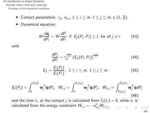
An Introduction to Impact Dynamics
Multiple impact restitution mappings
Summary of the dynamical equations
Contact parameters: γij , es,j , 1 ≤ i ≤ m, 1 ≤ j ≤ m, η (1, 32).
Dynamical equation:
Md q
dPi
= WdP
dPi
if Eji(Pj , Pi ) ≤ 1 for all j 6= i (43)
with
dPj
dPi
= γ1
η+1
ji (Eji (Pj , Pi ))η+1
η (44)
Eji =Ej(Pj)
Ei (Pi ), 1 ≤ i ≤ m, 1 ≤ j ≤ m (45)
Ej(Pj) =
∫ Pj (t)
0
wTj qdPj , Wr,j =
∫ Pj (tc )
0
wTj qdPj , Wc,j =
∫ Pj (tf )
Pj (tc )
wTj qdPj
(46)and the time tc at the contact j is calculated from δj(tc) = 0, while tf iscalculated from the energy constraint Wr,j = −e2
s,jWc,j .
187
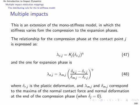
An Introduction to Impact Dynamics
Multiple impact restitution mappings
The distributing rule for the bi-stiffness model
Multiple impacts
This is an extension of the mono-stiffness model, in which thestiffness varies fom the compression to the expansion phases.
The relationship for the compression phase at the contact point jis expressed as:
λc,j = Kj(δc,j )η (47)
and the one for expansion phase is
λe,j = λm,j
(
δe,j − δr ,j
δm,j − δr ,j
)η
(48)
where δr ,j is the plastic deformation, and λm,j and δm,j correspondto the maxima of the normal contact force and normal deformationat the end of the compression phase (when δj = 0).
188
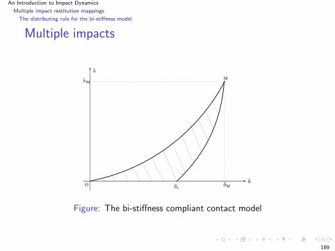
An Introduction to Impact Dynamics
Multiple impact restitution mappings
The distributing rule for the bi-stiffness model
Multiple impacts
M
M
M
r
Figure: The bi-stiffness compliant contact model
189
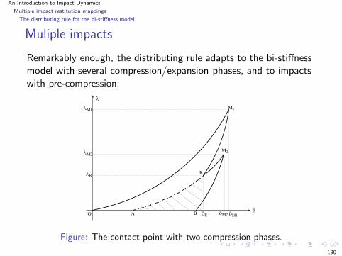
An Introduction to Impact Dynamics
Multiple impact restitution mappings
The distributing rule for the bi-stiffness model
Muliple impacts
Remarkably enough, the distributing rule adapts to the bi-stiffnessmodel with several compression/expansion phases, and to impactswith pre-compression:
M1
M2
M2
M1
A
M2
B
R
R M1
R
Figure: The contact point with two compression phases.
190
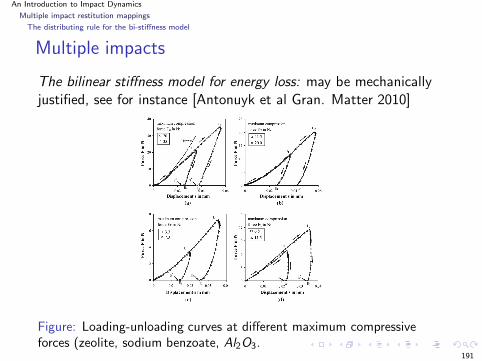
An Introduction to Impact Dynamics
Multiple impact restitution mappings
The distributing rule for the bi-stiffness model
Multiple impacts
The bilinear stiffness model for energy loss: may be mechanicallyjustified, see for instance [Antonuyk et al Gran. Matter 2010]
Figure: Loading-unloading curves at different maximum compressiveforces (zeolite, sodium benzoate, Al2O3.
191
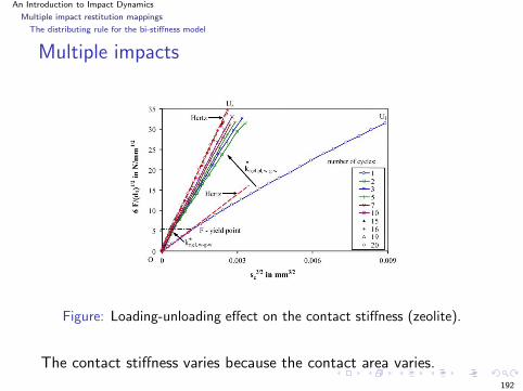
An Introduction to Impact Dynamics
Multiple impact restitution mappings
The distributing rule for the bi-stiffness model
Multiple impacts
Figure: Loading-unloading effect on the contact stiffness (zeolite).
The contact stiffness varies because the contact area varies.
192

An Introduction to Impact Dynamics
Multiple impact restitution mappings
Numerical results and comparisons with experiments
Multiple impacts
Numerical results have been obtained for:
Three-ball chains
Five-ball chains
Long chains (≥ 15 balls)
Bernoulli’s system
Columns of balls impacting a wall
and compared to either analytical results (when available) orexperimental results found in the literature:[Ceanga and Hurmuzlu, JAM 2001][Falcon et al, Europ. J. Phys. B, 1998]
193

An Introduction to Impact Dynamics
Multiple impact restitution mappings
Numerical results and comparisons with experiments
Multiple impacts
Let us consider the column of beads studied in [Falcon et al,Europ. J. Phys. B, 1998]:
1
N
h
g
Wall
Figure: A column of beads colliding against a wall.
194

An Introduction to Impact Dynamics
Multiple impact restitution mappings
Numerical results and comparisons with experiments
Multiple impacts
1 ≤ N ≤ 40 identical stainless steel beads, 8mm in diameter,2.05 ×10−3 kg.
“Wall” made of stainless steel.
Young modulus E = 21.6 × 10¹⁰ N/m2, Poisson ratioν = 0.276, for stainless steel
Contact stiffness bead/bead K = 6.9716 × 10⁹ N/m3/2
Contact stiffness bead/wall (sphere/plane) K = 9.858 × 10⁹
N/m3/2
Initial height h
The contact forces felt at the wall are recorded by a forcesensor.
Hertz elasticity
195
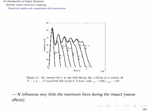
An Introduction to Impact Dynamics
Multiple impact restitution mappings
Numerical results and comparisons with experiments
N influences very little the maximum force during the impact (waves
effects).
196
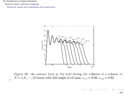
An Introduction to Impact Dynamics
Multiple impact restitution mappings
Numerical results and comparisons with experiments
197
An Introduction to Impact Dynamics
Multiple impact restitution mappings
Numerical results and comparisons with experiments
These results are very close (qualitatively and quantitatively) fromthe experimental ones of [Falcon et al, 1998]:
Experimental values: Fmax ≈ 52N for h = 3.1 mm,Fmax ≈ 71N for h = 5.1 mm
Experimental period of oscillation of the contact force≈ 32.4 ± 1µs (numerically ≈ 32µs) for h = 3.1 mm.
198
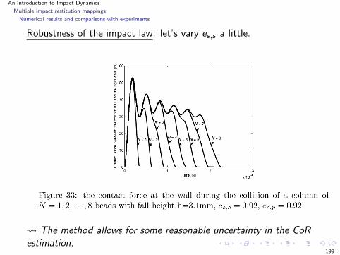
An Introduction to Impact Dynamics
Multiple impact restitution mappings
Numerical results and comparisons with experiments
Robustness of the impact law: let’s vary es,s a little.
The method allows for some reasonable uncertainty in the CoRestimation.
199
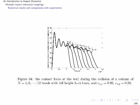
An Introduction to Impact Dynamics
Multiple impact restitution mappings
Numerical results and comparisons with experiments
200
An Introduction to Impact Dynamics
Multiple impacts with friction
Multiple impacts
The method extends to the case where there is friction at thecontacts. Has been successfully applied to the problem of abouncing dimer (a sort of small-scale rocking block).
References:
Z. Zhao, C. Liu, B. Brogliato, Physical Review E, 2008C. Liu, Z. Zhao, B. Brogliato, Proc. Royal Soc. A, 2008 and 2009Z. Zhao, C. Liu, B. Brogliato, Proc. Royal Soc. A, 2009
201
An Introduction to Impact Dynamics
Multiple impacts with friction
Wave effects
An important point for multiple impact modeling is: how may thestudies on waves in chains of balls be used in a multiple impact law?
For instance: [Nesterenko] solitary wave in a window of 5 ballswhen no pre-compression
most probably good parameters should be estimated fromgroups of 5 balls in the chain (if the chain is long enough)
Problem: high sensitivity w.r.t. initial data (initial velocities andinitial pre-compression, type of elasticity – linear or nonlinear–)
However it seems that much more has to be done on wavesanalysis to be able to really enrich a multiple impact law with some“macroscopic” model that reflects the waves transmissionsthroughout the chain, for any initial data.
202


![A Matrix Method for Efficient Computation of Bernstein ... · [10] reintroduces the binomial coefficients while computing the Bernstein coefficients, hence is inefficient for directly](https://static.documents.pub/doc/80x56/6008a4318b88952825139498/a-matrix-method-for-eifcient-computation-of-bernstein-10-reintroduces-the.jpg)


