An Introduction to Machine Learning L4: Support Vector Classification Alexander J. Smola Statistical Machine Learning Program Canberra, ACT 0200 Australia [email protected]Tata Institute, Pune, January 2007 Alexander J. Smola: An Introduction to Machine Learning 1 / 77
Transcript
An Introduction to Machine LearningL4: Support Vector Classification
Alexander J. Smola
Statistical Machine Learning ProgramCanberra, ACT 0200 Australia
Alexander J. Smola: An Introduction to Machine Learning 1 / 77
Overview
L1: Machine learning and probability theoryIntroduction to pattern recognition, classification, regression,novelty detection, probability theory, Bayes rule, inference
L2: Density estimation and Parzen windowsNearest Neighbor, Kernels density estimation, Silverman’srule, Watson Nadaraya estimator, crossvalidation
L3: Perceptron and KernelsHebb’s rule, perceptron algorithm, convergence, kernels
L4: Support Vector estimationGeometrical view, dual problem, convex optimization, kernels
L5: Support Vector estimationRegression, Quantile regression, Novelty detection, ν-trick
L6: Structured EstimationSequence annotation, web page ranking, path planning,implementation and optimization
Alexander J. Smola: An Introduction to Machine Learning 2 / 77
L4 Support Vector Classification
Support Vector MachineProblem definitionGeometrical pictureOptimization problem
Optimization ProblemHard marginConvexityDual problemSoft margin problem
Alexander J. Smola: An Introduction to Machine Learning 3 / 77
Classification
DataPairs of observations (xi , yi) generated from somedistribution P(x , y), e.g., (blood status, cancer), (credittransaction, fraud), (profile of jet engine, defect)
TaskEstimate y given x at a new location.Modification: find a function f (x) that does the task.
Alexander J. Smola: An Introduction to Machine Learning 4 / 77
So Many Solutions
Alexander J. Smola: An Introduction to Machine Learning 5 / 77
One to rule them all . . .
Alexander J. Smola: An Introduction to Machine Learning 6 / 77
Optimal Separating Hyperplane
Alexander J. Smola: An Introduction to Machine Learning 7 / 77
Optimization Problem
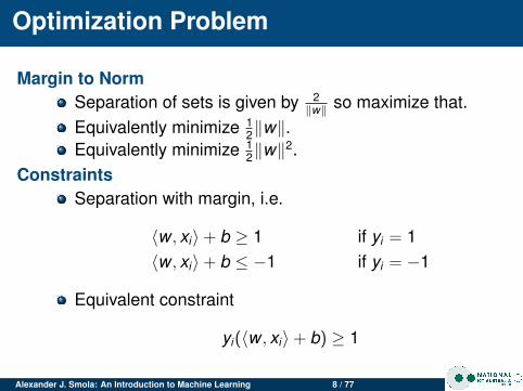
Margin to NormSeparation of sets is given by 2
‖w‖ so maximize that.Equivalently minimize 1
2‖w‖.Equivalently minimize 1
2‖w‖2.
ConstraintsSeparation with margin, i.e.
〈w , xi〉+ b ≥ 1 if yi = 1〈w , xi〉+ b ≤ −1 if yi = −1
Equivalent constraint
yi(〈w , xi〉+ b) ≥ 1
Alexander J. Smola: An Introduction to Machine Learning 8 / 77
Optimization Problem
Mathematical Programming SettingCombining the above requirements we obtain
minimize12‖w‖2
subject to yi(〈w , xi〉+ b)− 1 ≥ 0 for all 1 ≤ i ≤ m
PropertiesProblem is convexHence it has unique minimumEfficient algorithms for solving it exist
Alexander J. Smola: An Introduction to Machine Learning 9 / 77
Lagrange Function
Objective Function12‖w‖2.
Constraints ci(w , b) := 1− yi(〈w , xi〉+ b) ≤ 0Lagrange Function
L(w , b, α) = PrimalObjective +∑
i
αici
=12‖w‖2 +
m∑i=1
αi(1− yi(〈w , xi〉+ b))
Saddle Point ConditionDerivatives of L with respect to w and b must vanish.
Alexander J. Smola: An Introduction to Machine Learning 10 / 77
Support Vector Machines
Optimization Problem
minimize12
m∑i,j=1
αiαjyiyj〈xi , xj〉−m∑
i=1
αi
subject tom∑
i=1
αiyi = 0 and αi ≥ 0
Support Vector Expansion
w =∑
i
αiyixi and hence f (x) =m∑
i=1
αiyi 〈xi , x〉+ b
Kuhn Tucker Conditions
αi(1− yi(〈xi , x〉+ b)) = 0
Alexander J. Smola: An Introduction to Machine Learning 11 / 77
Proof (optional)
Lagrange Function
L(w , b, α) =12‖w‖2 +
m∑i=1
αi(1− yi(〈w , xi〉+ b))
Saddlepoint condition
∂wL(w , b, α) = w −m∑
i=1
αiyixi = 0 ⇐⇒ w =m∑
i=1
αiyixi
∂bL(w , b, α) = −m∑
i=1
αiyixi = 0 ⇐⇒m∑
i=1
αiyi = 0
To obtain the dual optimization problem we have to substitutethe values of w and b into L. Note that the dual variables αi
have the constraint αi ≥ 0.Alexander J. Smola: An Introduction to Machine Learning 12 / 77
Proof (optional)
Dual Optimization ProblemAfter substituting in terms for b, w the Lagrange functionbecomes
− 12
m∑i,j=1
αiαjyiyj〈xi , xj〉+m∑
i=1
αi
subject tom∑
i=1
αiyi = 0 and αi ≥ 0 for all 1 ≤ i ≤ m
Practical ModificationNeed to maximize dual objective function. Rewrite as
minimize12
m∑i,j=1
αiαjyiyj〈xi , xj〉 −m∑
i=1
αi
subject to the above constraints.Alexander J. Smola: An Introduction to Machine Learning 13 / 77
Support Vector Expansion
Solution in w =m∑
i=1
αiyixi
w is given by a linear combination of training patterns xi .Independent of the dimensionality of x .w depends on the Lagrange multipliers αi .
Kuhn-Tucker-ConditionsAt optimal solution Constraint · Lagrange Multiplier = 0In our context this means
αi(1− yi(〈w , xi〉+ b)) = 0.
Equivalently we have
αi 6= 0 ⇐⇒ yi (〈w , xi〉+ b) = 1
Only points at the decision boundary can contributeto the solution.
Alexander J. Smola: An Introduction to Machine Learning 14 / 77
Mini Summary
Linear ClassificationMany solutionsOptimal separating hyperplaneOptimization problem
Support Vector MachinesQuadratic problemLagrange functionDual problem
InterpretationDual variables and SVsSV expansionHard margin and infinite weights
Alexander J. Smola: An Introduction to Machine Learning 15 / 77
Kernels
Nonlinearity via Feature MapsReplace xi by Φ(xi) in the optimization problem.
Equivalent optimization problem
minimize12
m∑i,j=1
αiαjyiyjk(xi , xj)−m∑
i=1
αi
subject tom∑
i=1
αiyi = 0 and αi ≥ 0
Decision Function
w =m∑
i=1
αiyiΦ(xi) implies
f (x) = 〈w , Φ(x)〉+ b =m∑
i=1
αiyik(xi , x) + b.
Alexander J. Smola: An Introduction to Machine Learning 16 / 77
Examples and Problems
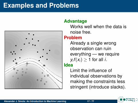
AdvantageWorks well when the data isnoise free.
ProblemAlready a single wrongobservation can ruineverything — we requireyi f (xi) ≥ 1 for all i .
IdeaLimit the influence ofindividual observations bymaking the constraints lessstringent (introduce slacks).
Alexander J. Smola: An Introduction to Machine Learning 17 / 77
Optimization Problem (Soft Margin)
Recall: Hard Margin Problem
minimize12‖w‖2
subject to yi(〈w , xi〉+ b)− 1 ≥ 0
Softening the Constraints
minimize12‖w‖2 + C
m∑i=1
ξi
subject to yi(〈w , xi〉+ b)− 1+ξi ≥ 0 and ξi ≥ 0
Alexander J. Smola: An Introduction to Machine Learning 18 / 77
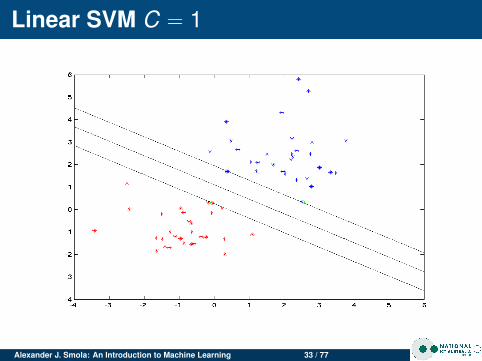
Linear SVM C = 1
Alexander J. Smola: An Introduction to Machine Learning 19 / 77
Linear SVM C = 2
Alexander J. Smola: An Introduction to Machine Learning 20 / 77
Linear SVM C = 5
Alexander J. Smola: An Introduction to Machine Learning 21 / 77
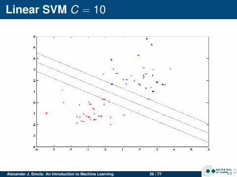
Linear SVM C = 10
Alexander J. Smola: An Introduction to Machine Learning 22 / 77
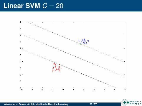
Linear SVM C = 20
Alexander J. Smola: An Introduction to Machine Learning 23 / 77
Linear SVM C = 50
Alexander J. Smola: An Introduction to Machine Learning 24 / 77
Linear SVM C = 100
Alexander J. Smola: An Introduction to Machine Learning 25 / 77
Linear SVM C = 1
Alexander J. Smola: An Introduction to Machine Learning 26 / 77
Linear SVM C = 2
Alexander J. Smola: An Introduction to Machine Learning 27 / 77
Linear SVM C = 5
Alexander J. Smola: An Introduction to Machine Learning 28 / 77
Linear SVM C = 10
Alexander J. Smola: An Introduction to Machine Learning 29 / 77
Linear SVM C = 20
Alexander J. Smola: An Introduction to Machine Learning 30 / 77
Linear SVM C = 50
Alexander J. Smola: An Introduction to Machine Learning 31 / 77
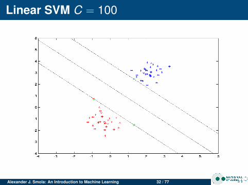
Linear SVM C = 100
Alexander J. Smola: An Introduction to Machine Learning 32 / 77
Linear SVM C = 1
Alexander J. Smola: An Introduction to Machine Learning 33 / 77
Linear SVM C = 2
Alexander J. Smola: An Introduction to Machine Learning 34 / 77
Linear SVM C = 5
Alexander J. Smola: An Introduction to Machine Learning 35 / 77
Linear SVM C = 10
Alexander J. Smola: An Introduction to Machine Learning 36 / 77
Linear SVM C = 20
Alexander J. Smola: An Introduction to Machine Learning 37 / 77
Linear SVM C = 50
Alexander J. Smola: An Introduction to Machine Learning 38 / 77
Linear SVM C = 100
Alexander J. Smola: An Introduction to Machine Learning 39 / 77
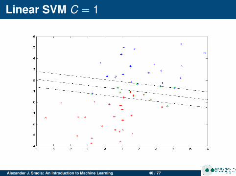
Linear SVM C = 1
Alexander J. Smola: An Introduction to Machine Learning 40 / 77
Linear SVM C = 2
Alexander J. Smola: An Introduction to Machine Learning 41 / 77
Linear SVM C = 5
Alexander J. Smola: An Introduction to Machine Learning 42 / 77
Linear SVM C = 10
Alexander J. Smola: An Introduction to Machine Learning 43 / 77
Linear SVM C = 20
Alexander J. Smola: An Introduction to Machine Learning 44 / 77
Linear SVM C = 50
Alexander J. Smola: An Introduction to Machine Learning 45 / 77
Linear SVM C = 100
Alexander J. Smola: An Introduction to Machine Learning 46 / 77
Insights
Changing CFor clean data C doesn’t matter much.For noisy data, large C leads to narrow margin (SVMtries to do a good job at separating, even though it isn’tpossible)
Noisy dataClean data has few support vectorsNoisy data leads to data in the marginsMore support vectors for noisy data
Alexander J. Smola: An Introduction to Machine Learning 47 / 77
Alexander J. Smola: An Introduction to Machine Learning 48 / 77
Dual Optimization Problem
Optimization Problem
minimize12
m∑i,j=1
αiαjyiyjk(xi , xj)−m∑
i=1
αi
subject tom∑
i=1
αiyi = 0 and C ≥ αi ≥ 0 for all 1 ≤ i ≤ m
InterpretationAlmost same optimization problem as beforeConstraint on weight of each αi (bounds influence ofpattern).Efficient solvers exist (more about that tomorrow).
Alexander J. Smola: An Introduction to Machine Learning 49 / 77
SV Classification Machine
Alexander J. Smola: An Introduction to Machine Learning 50 / 77
Gaussian RBF with C = 0.1
Alexander J. Smola: An Introduction to Machine Learning 51 / 77
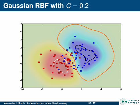
Gaussian RBF with C = 0.2
Alexander J. Smola: An Introduction to Machine Learning 52 / 77
Gaussian RBF with C = 0.4
Alexander J. Smola: An Introduction to Machine Learning 53 / 77
Gaussian RBF with C = 0.8
Alexander J. Smola: An Introduction to Machine Learning 54 / 77
Gaussian RBF with C = 1.6
Alexander J. Smola: An Introduction to Machine Learning 55 / 77
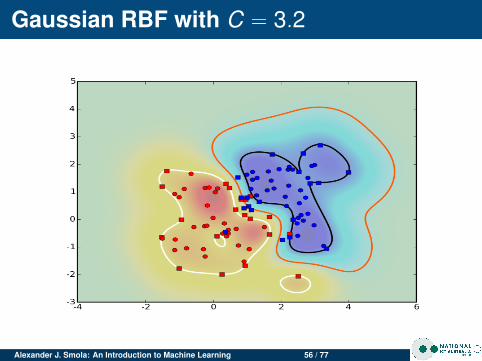
Gaussian RBF with C = 3.2
Alexander J. Smola: An Introduction to Machine Learning 56 / 77
Gaussian RBF with C = 6.4
Alexander J. Smola: An Introduction to Machine Learning 57 / 77
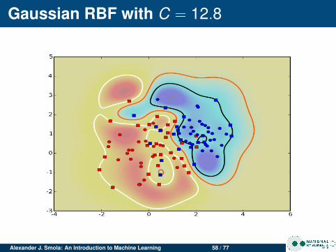
Gaussian RBF with C = 12.8
Alexander J. Smola: An Introduction to Machine Learning 58 / 77
Insights
Changing CFor clean data C doesn’t matter much.For noisy data, large C leads to more complicatedmargin (SVM tries to do a good job at separating, eventhough it isn’t possible)Overfitting for large C
Noisy dataClean data has few support vectorsNoisy data leads to data in the marginsMore support vectors for noisy data
Alexander J. Smola: An Introduction to Machine Learning 59 / 77
Gaussian RBF with σ = 1
Alexander J. Smola: An Introduction to Machine Learning 60 / 77
Gaussian RBF with σ = 2
Alexander J. Smola: An Introduction to Machine Learning 61 / 77
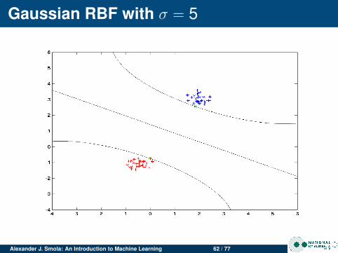
Gaussian RBF with σ = 5
Alexander J. Smola: An Introduction to Machine Learning 62 / 77
Gaussian RBF with σ = 10
Alexander J. Smola: An Introduction to Machine Learning 63 / 77
Gaussian RBF with σ = 1
Alexander J. Smola: An Introduction to Machine Learning 64 / 77
Gaussian RBF with σ = 2
Alexander J. Smola: An Introduction to Machine Learning 65 / 77
Gaussian RBF with σ = 5
Alexander J. Smola: An Introduction to Machine Learning 66 / 77
Gaussian RBF with σ = 10
Alexander J. Smola: An Introduction to Machine Learning 67 / 77
Gaussian RBF with σ = 1
Alexander J. Smola: An Introduction to Machine Learning 68 / 77
Gaussian RBF with σ = 2
Alexander J. Smola: An Introduction to Machine Learning 69 / 77
Gaussian RBF with σ = 5
Alexander J. Smola: An Introduction to Machine Learning 70 / 77
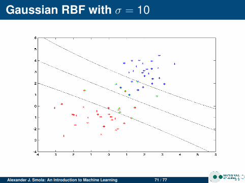
Gaussian RBF with σ = 10
Alexander J. Smola: An Introduction to Machine Learning 71 / 77
Gaussian RBF with σ = 1
Alexander J. Smola: An Introduction to Machine Learning 72 / 77
Gaussian RBF with σ = 2
Alexander J. Smola: An Introduction to Machine Learning 73 / 77
Gaussian RBF with σ = 5
Alexander J. Smola: An Introduction to Machine Learning 74 / 77
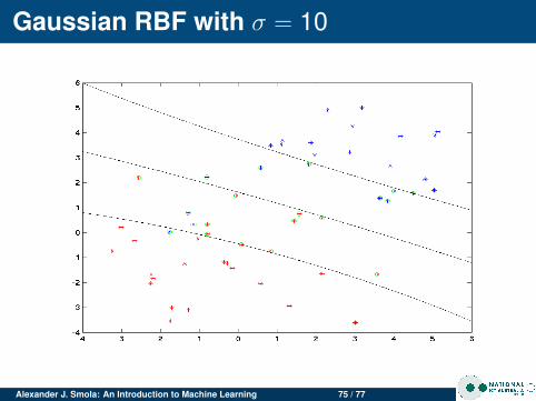
Gaussian RBF with σ = 10
Alexander J. Smola: An Introduction to Machine Learning 75 / 77
Insights
Changing σ
For clean data σ doesn’t matter much.For noisy data, small σ leads to more complicatedmargin (SVM tries to do a good job at separating, eventhough it isn’t possible)Lots of overfitting for small σ
Noisy dataClean data has few support vectorsNoisy data leads to data in the marginsMore support vectors for noisy data
Alexander J. Smola: An Introduction to Machine Learning 76 / 77
Summary
Support Vector MachineProblem definitionGeometrical pictureOptimization problem
Optimization ProblemHard marginConvexityDual problemSoft margin problem
Alexander J. Smola: An Introduction to Machine Learning 77 / 77