Alexander J. Smola: An Introduction to Machine Learning with Kernels, Page 1 An Introduction to Machine Learning with Kernels Lecture 3 Alexander J. Smola [email protected]Statistical Machine Learning Program National ICT Australia, Canberra
Transcript
Alexander J. Smola: An Introduction to Machine Learning with Kernels, Page 1
Alexander J. Smola: An Introduction to Machine Learning with Kernels, Page 2
Machine learning and probability theoryIntroduction to pattern recognition, classification, regres-sion, novelty detection, probability theory, Bayes rule, in-ference
Density estimation and Parzen windowsKernels and density estimation, Silverman’s rule, Wat-son Nadaraya estimator, crossvalidation
FeaturesExplicit feature constructionImplicit features via kernels
KernelsExamplesKernel perceptron
Biology and Learning
Alexander J. Smola: An Introduction to Machine Learning with Kernels, Page 4
Basic IdeaGood behavior should be rewarded, bad behaviorpunished (or not rewarded). This improves the fitnessof the system.Example: hitting a sabertooth tiger over the headshould be rewarded . . .Correlated events should be combined.Example: Pavlov’s salivating dog.
Training MechanismsBehavioral modification of individuals (learning) —successful behavior is rewarded (e.g. food).Hard-coded behavior in the genes (instinct) — thewrongly coded animal dies.
Neurons
Alexander J. Smola: An Introduction to Machine Learning with Kernels, Page 5
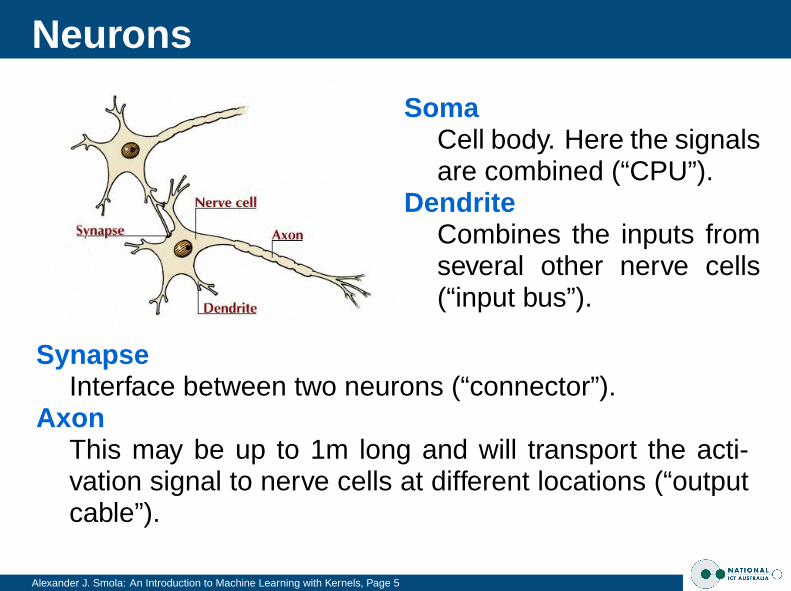
SomaCell body. Here the signalsare combined (“CPU”).
DendriteCombines the inputs fromseveral other nerve cells(“input bus”).
SynapseInterface between two neurons (“connector”).
AxonThis may be up to 1m long and will transport the acti-vation signal to nerve cells at different locations (“outputcable”).
Perceptron
Alexander J. Smola: An Introduction to Machine Learning with Kernels, Page 6
Perceptrons
Alexander J. Smola: An Introduction to Machine Learning with Kernels, Page 7
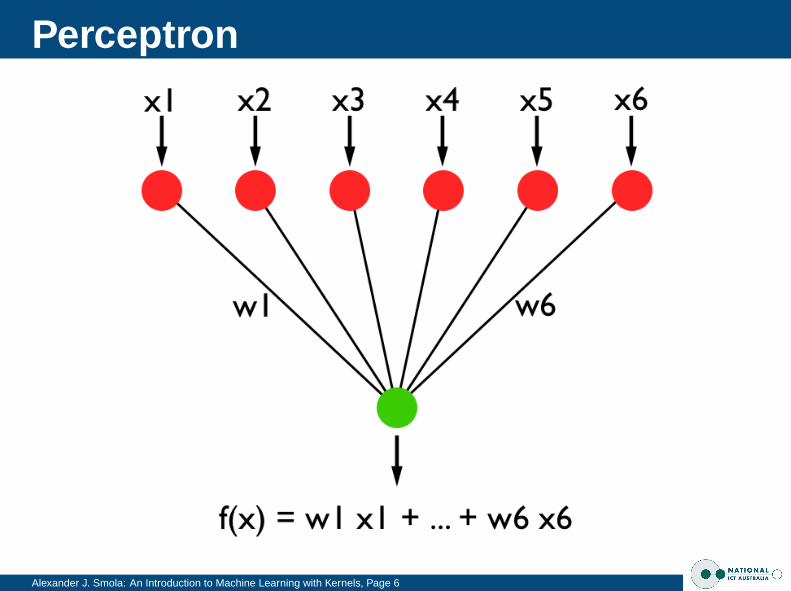
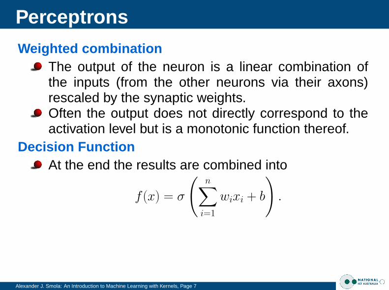
Weighted combinationThe output of the neuron is a linear combination ofthe inputs (from the other neurons via their axons)rescaled by the synaptic weights.Often the output does not directly correspond to theactivation level but is a monotonic function thereof.
Decision FunctionAt the end the results are combined into
f (x) = σ
(n∑
i=1
wixi + b
).
Separating Half Spaces
Alexander J. Smola: An Introduction to Machine Learning with Kernels, Page 8
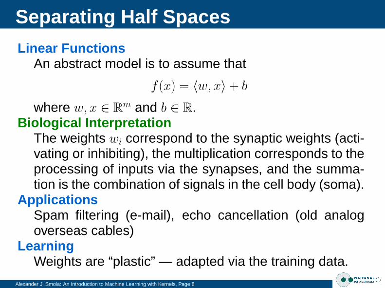
Linear FunctionsAn abstract model is to assume that
f (x) = 〈w, x〉 + b
where w, x ∈ Rm and b ∈ R.Biological Interpretation
The weights wi correspond to the synaptic weights (acti-vating or inhibiting), the multiplication corresponds to theprocessing of inputs via the synapses, and the summa-tion is the combination of signals in the cell body (soma).
function (w, b) = Perceptron(X, Y )initialize w, b = 0repeat
Pick (xi, yi) from dataif yi(w · xi + b) ≤ 0 then
w′ = w + yixi
b′ = b + yi
until yi(w · xi + b) > 0 for all iend
Interpretation
Alexander J. Smola: An Introduction to Machine Learning with Kernels, Page 11
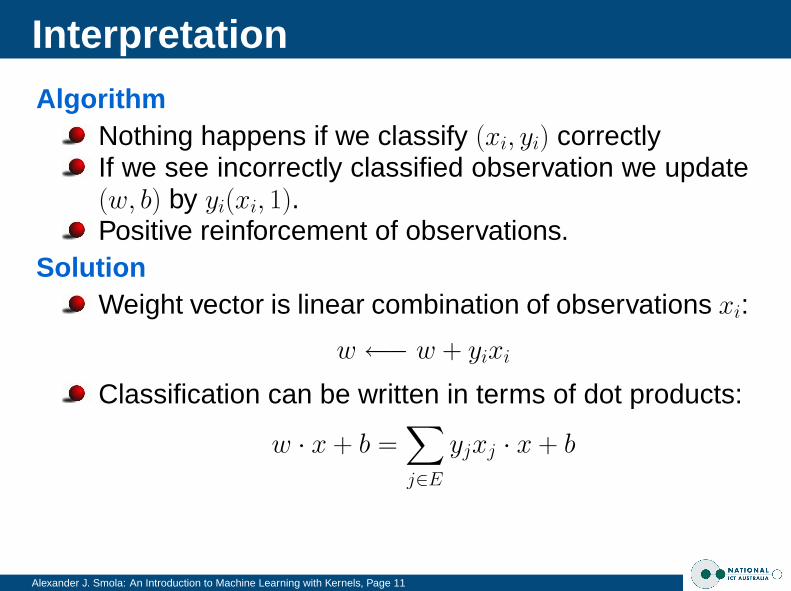
AlgorithmNothing happens if we classify (xi, yi) correctlyIf we see incorrectly classified observation we update(w, b) by yi(xi, 1).Positive reinforcement of observations.
SolutionWeight vector is linear combination of observations xi:
w ←− w + yixi
Classification can be written in terms of dot products:
w · x + b =∑j∈E
yjxj · x + b
Theoretical Analysis
Alexander J. Smola: An Introduction to Machine Learning with Kernels, Page 12
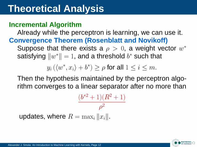
Incremental AlgorithmAlready while the perceptron is learning, we can use it.
Convergence Theorem (Rosenblatt and Novikoff)Suppose that there exists a ρ > 0, a weight vector w∗
satisfying ‖w∗‖ = 1, and a threshold b∗ such that
yi (〈w∗, xi〉 + b∗) ≥ ρ for all 1 ≤ i ≤ m.
Then the hypothesis maintained by the perceptron algo-rithm converges to a linear separator after no more than
(b∗2 + 1)(R2 + 1)
ρ2
updates, where R = maxi ‖xi‖.
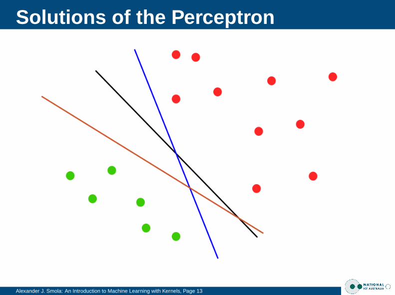
Solutions of the Perceptron
Alexander J. Smola: An Introduction to Machine Learning with Kernels, Page 13
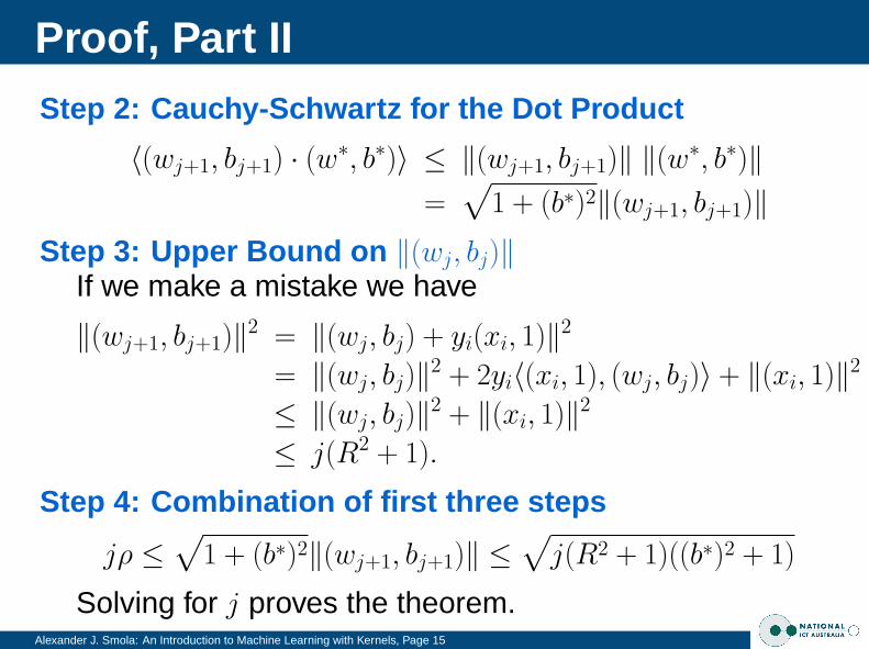
Proof, Part I
Alexander J. Smola: An Introduction to Machine Learning with Kernels, Page 14
Starting PointWe start from w1 = 0 and b1 = 0.
Step 1: Bound on the increase of alignmentDenote by wi the value of w at step i (analogously bi).
Alexander J. Smola: An Introduction to Machine Learning with Kernels, Page 16
Learning AlgorithmWe perform an update only if we make a mistake.
Convergence BoundBounds the maximum number of mistakes in total.We will make at most (b∗2 + 1)(R1 + 1)/ρ2 mistakes inthe case where a “correct” solution w∗, b∗ exists.This also bounds the expected error (if we know ρ, R,and |b∗|).
Dimension IndependentBound does not depend on the dimensionality of X.
Sample ExpansionWe obtain x as a linear combination of xi.
Realizable and Non-realizable Concepts
Alexander J. Smola: An Introduction to Machine Learning with Kernels, Page 17
Realizable ConceptHere some w∗, b∗ exists such that y is generated byy = sgn (〈w∗, x〉 + b). In general realizable means thatthe exact functional dependency is included in the classof admissible hypotheses.
Unrealizable ConceptIn this case, the exact concept does not exist or it is notincluded in the function class.
The XOR Problem
Alexander J. Smola: An Introduction to Machine Learning with Kernels, Page 18
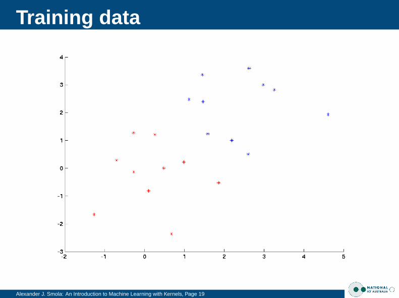
Training data
Alexander J. Smola: An Introduction to Machine Learning with Kernels, Page 19
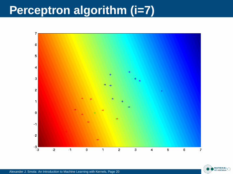
Perceptron algorithm (i=7)
Alexander J. Smola: An Introduction to Machine Learning with Kernels, Page 20
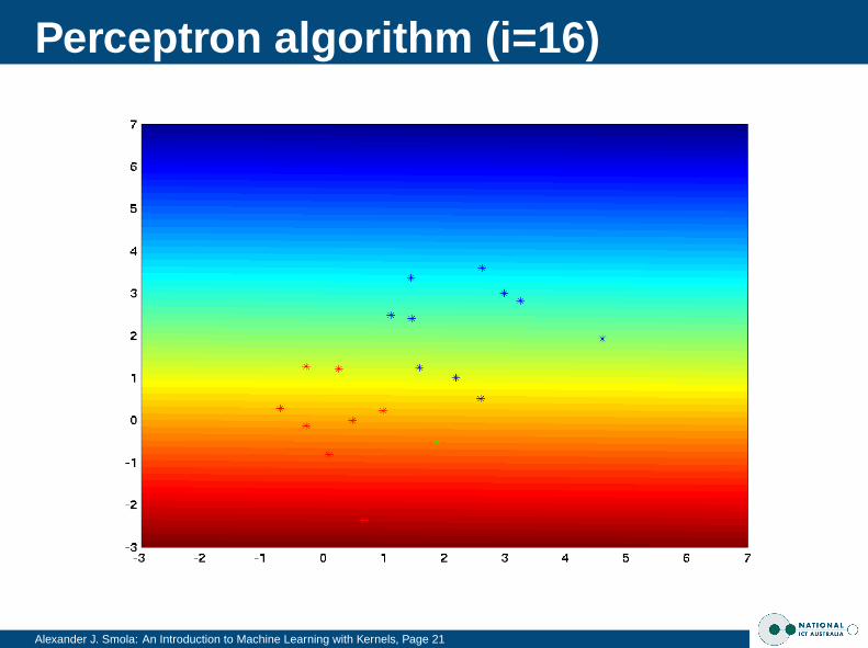
Perceptron algorithm (i=16)
Alexander J. Smola: An Introduction to Machine Learning with Kernels, Page 21
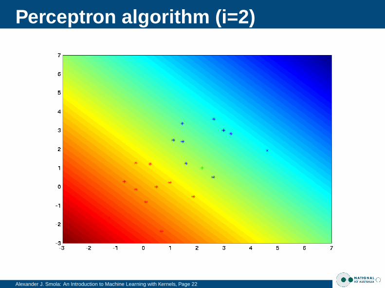
Perceptron algorithm (i=2)
Alexander J. Smola: An Introduction to Machine Learning with Kernels, Page 22
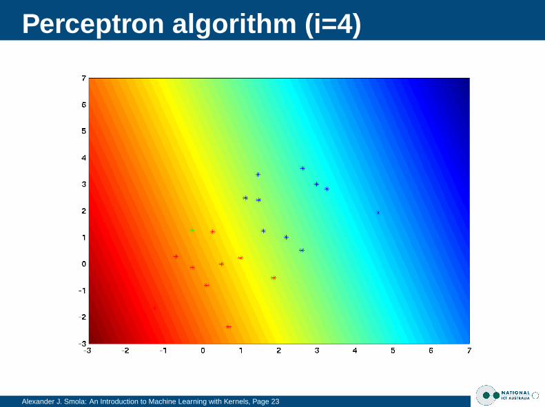
Perceptron algorithm (i=4)
Alexander J. Smola: An Introduction to Machine Learning with Kernels, Page 23
Perceptron algorithm (i=16)
Alexander J. Smola: An Introduction to Machine Learning with Kernels, Page 24
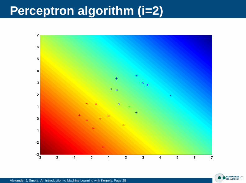
Perceptron algorithm (i=2)
Alexander J. Smola: An Introduction to Machine Learning with Kernels, Page 25
Perceptron algorithm (i=16)
Alexander J. Smola: An Introduction to Machine Learning with Kernels, Page 26
Perceptron algorithm (i=12)
Alexander J. Smola: An Introduction to Machine Learning with Kernels, Page 27
Perceptron algorithm (i=16)
Alexander J. Smola: An Introduction to Machine Learning with Kernels, Page 28
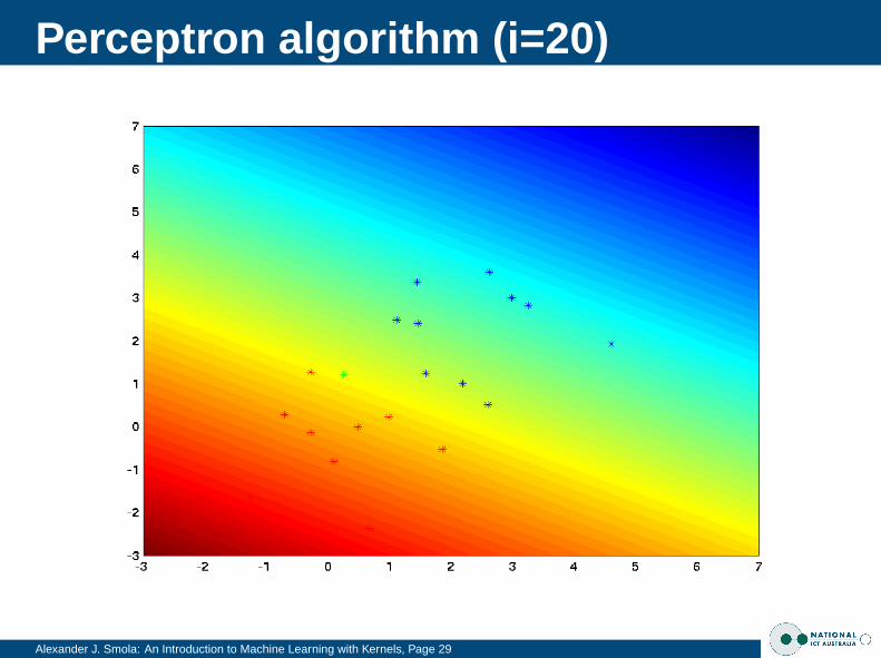
Perceptron algorithm (i=20)
Alexander J. Smola: An Introduction to Machine Learning with Kernels, Page 29
Stochastic Gradient Descent, 1
Alexander J. Smola: An Introduction to Machine Learning with Kernels, Page 30
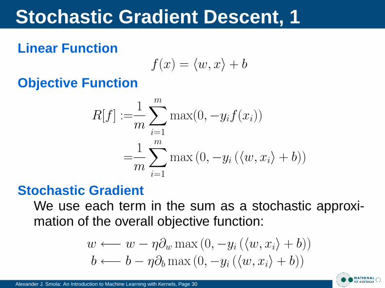
Linear Functionf (x) = 〈w, x〉 + b
Objective Function
R[f ] :=1
m
m∑i=1
max(0,−yif (xi))
=1
m
m∑i=1
max (0,−yi (〈w, xi〉 + b))
Stochastic GradientWe use each term in the sum as a stochastic approxi-mation of the overall objective function:
w ←− w − η∂w max (0,−yi (〈w, xi〉 + b))
b←− b− η∂b max (0,−yi (〈w, xi〉 + b))
Stochastic Gradient Descent, 2
Alexander J. Smola: An Introduction to Machine Learning with Kernels, Page 31
Details
∂w max (0,−yi (〈w, xi〉 + b)) =
{−yixi for yif (xi) < 00 otherwise
∂b max (0,−yi (〈w, xi〉 + b)) =
{−yi for yif (xi) < 00 otherwise
Overall StrategyHave complicated function consisting of lots of termsWant to minimize this monsterSolve it performing descent into one direction at a timeRandomly pick directions and convergeOften need to adjust learning rate η
η =C
t + Ttypically T ∼ 1000, C ∼ 10000
Mini Summary
Alexander J. Smola: An Introduction to Machine Learning with Kernels, Page 32
PerceptronSeparating halfspacesPerceptron algorithmConvergence theoremOnly depends on margin, dimension independent
Stochastic Gradient DescentStochastic approximationGradient descent gives perceptron for hinge lossWorks for other problems, too
Nonlinearity via Preprocessing
Alexander J. Smola: An Introduction to Machine Learning with Kernels, Page 33
ProblemLinear functions are often too simple to provide good es-timators.
IdeaMap to a higher dimensional feature space via Φ : x→Φ(x) and solve the problem there.Replace every 〈x, x′〉 by 〈Φ(x), Φ(x′)〉 in the perceptronalgorithm.
ConsequenceWe have nonlinear classifiers.Solution lies in the choice of features Φ(x).
Nonlinearity via Preprocessing
Alexander J. Smola: An Introduction to Machine Learning with Kernels, Page 34
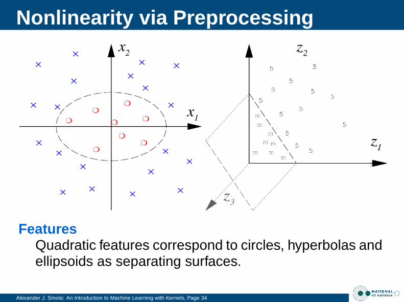
FeaturesQuadratic features correspond to circles, hyperbolas andellipsoids as separating surfaces.
Constructing Features
Alexander J. Smola: An Introduction to Machine Learning with Kernels, Page 35
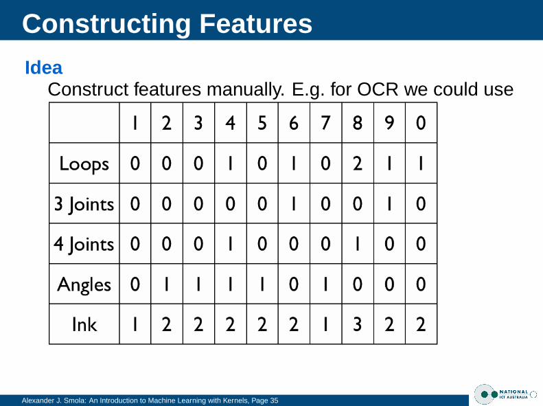
IdeaConstruct features manually. E.g. for OCR we could use
More Examples
Alexander J. Smola: An Introduction to Machine Learning with Kernels, Page 36
Two Interlocking SpiralsIf we transform the data (x1, x2) into a radial part (r =√
x21 + x2
2) and an angular part (x1 = r cos φ, x1 = r sin φ),the problem becomes much easier to solve (we onlyhave to distinguish different stripes).
Japanese Character RecognitionBreak down the images into strokes and recognize itfrom the latter (there’s a predefined order of them).
Medical DiagnosisInclude physician’s comments, knowledge about un-healthy combinations, features in EEG, . . .
Suitable RescalingIf we observe, say the weight and the height of a person,rescale to zero mean and unit variance.
Perceptron on Features
Alexander J. Smola: An Introduction to Machine Learning with Kernels, Page 37
function (w, b) = Perceptron(X, Y, η)initialize w, b = 0repeat
Pick (xi, yi) from dataif yi(w · Φ(xi) + b) ≤ 0 then
w′ = w + yiΦ(xi)b′ = b + yi
until yi(w · Φ(xi) + b) > 0 for all iend
Important detailw =
∑j
yjΦ(xj) and hence f (x) =∑
j yj(Φ(xj) · Φ(x)) + b
Problems with Constructing Features
Alexander J. Smola: An Introduction to Machine Learning with Kernels, Page 38
ProblemsNeed to be an expert in the domain (e.g. Chinesecharacters).Features may not be robust (e.g. postman drops letterin dirt).Can be expensive to compute.
SolutionUse shotgun approach.Compute many features and hope a good one isamong them.Do this efficiently.
Polynomial Features
Alexander J. Smola: An Introduction to Machine Learning with Kernels, Page 39
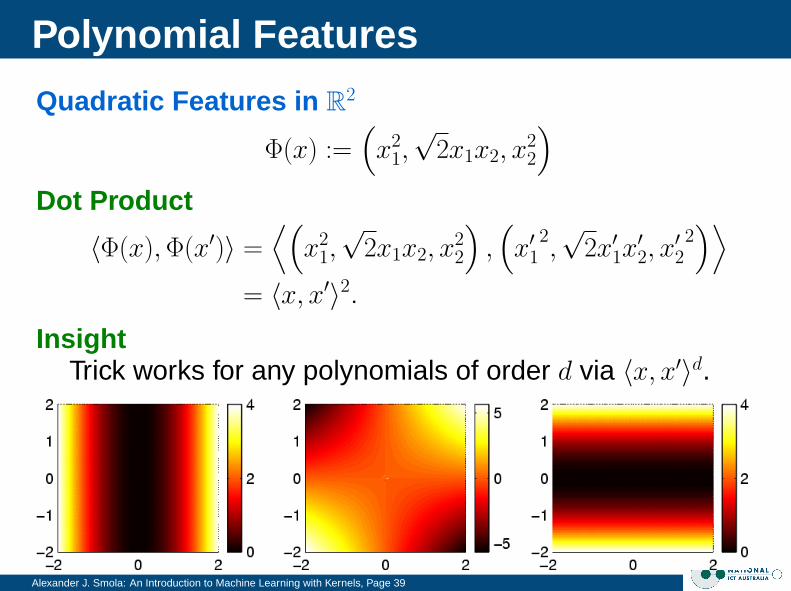
Quadratic Features in R2
Φ(x) :=(x2
1,√
2x1x2, x22
)Dot Product
〈Φ(x), Φ(x′)〉 =⟨(
x21,√
2x1x2, x22
),(x′1
2,√
2x′1x′2, x′22)⟩
= 〈x, x′〉2.Insight
Trick works for any polynomials of order d via 〈x, x′〉d.
Kernels
Alexander J. Smola: An Introduction to Machine Learning with Kernels, Page 40
ProblemExtracting features can sometimes be very costly.Example: second order features in 1000 dimensions.This leads to 5005 numbers. For higher order polyno-mial features much worse.
SolutionDon’t compute the features, try to compute dot productsimplicitly. For some features this works . . .
DefinitionA kernel function k : X× X → R is a symmetric functionin its arguments for which the following property holds
k(x, x′) = 〈Φ(x), Φ(x′)〉 for some feature map Φ.
If k(x, x′) is much cheaper to compute than Φ(x) . . .
Polynomial Kernels in Rn
Alexander J. Smola: An Introduction to Machine Learning with Kernels, Page 41
IdeaWe want to extend k(x, x′) = 〈x, x′〉2 to
k(x, x′) = (〈x, x′〉 + c)d where c > 0 and d ∈ N.
Prove that such a kernel corresponds to a dot product.Proof strategy
Simple and straightforward: compute the explicit sumgiven by the kernel, i.e.
k(x, x′) = (〈x, x′〉 + c)d
=
m∑i=0
(d
i
)(〈x, x′〉)i cd−i
Individual terms (〈x, x′〉)i are dot products for some Φi(x).
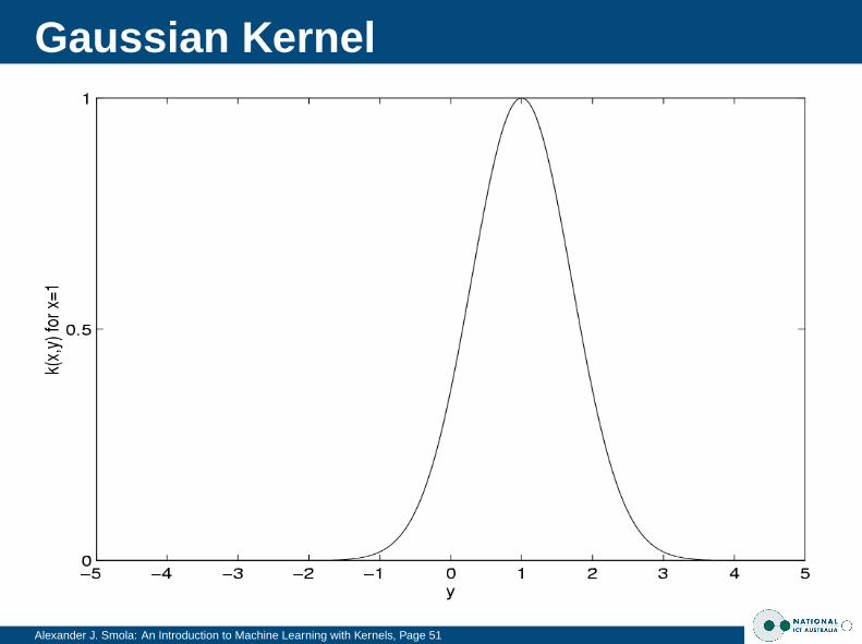
Kernel Perceptron
Alexander J. Smola: An Introduction to Machine Learning with Kernels, Page 42