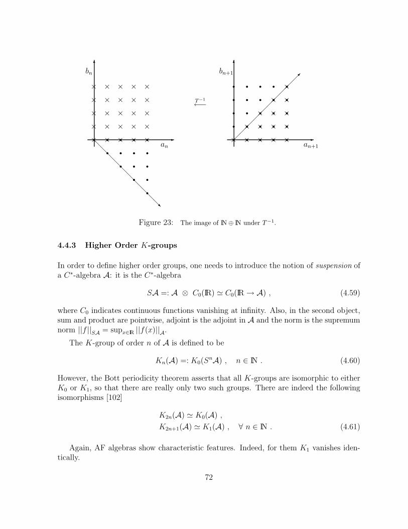
arXiv:hep-th/9701078v1 16 Jan 1997 An Introduction to Noncommutative Spaces and their Geometry Giovanni Landi Dipartimento di Scienze Matematiche, Universit` a di Trieste, P.le Europa 1, I-34127, Trieste, Italia. INFN, Sezione di Napoli, Mostra d’ Oltremare pad. 20, I-80125, Napoli, Italia. Trieste, January 16, 1997 hep-th/9701078
Transcript
arX
iv:h
ep-t
h/97
0107
8v1
16
Jan
1997
An Introduction to
Noncommutative Spaces and their Geometry
Giovanni Landi
Dipartimento di Scienze Matematiche, Universita di Trieste,P.le Europa 1, I-34127, Trieste, Italia.
INFN, Sezione di Napoli,Mostra d’ Oltremare pad. 20, I-80125, Napoli, Italia.
10 Quantum Mechanical Models on Noncommutative Lattices 148
A Basic Notions of Topology 152
B The Gel’fand-Naimark-Segal Construction 155
C Hilbert Modules 158
D Strong Morita Equivalence 164
E Partially Ordered Sets 167
F Pseudodifferential Operators 170
iii
Preface
These notes arose from a series of introductory seminars on noncommutative geometry Igave at the University of Trieste in September 1995 during the X Workshop on DifferentialGeometric Methods in Classical Mechanics. It was Beppe Marmo’s suggestion that I wrotenotes of the lectures.
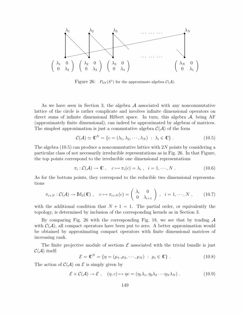
The notes are mainly an introduction to Connes’ noncommutative geometry. Theycould serve as a ‘first aid kit’ before one ventures into the beautiful but bewilderinglandscape of Connes’ theory [25]. The main difference with other available introductionsto Connes’s work, notably Kastler’s papers [65] and also Gracia-Bondıa and Varilly paper[101], is the emphasis on noncommutative spaces seen as concrete spaces.
Important examples of noncommutative spaces are provided by noncommutative lat-tices. The latter are the subject of intensive work I am doing in collaboration with A.P.Balachandran, Giuseppe Bimonte, Elisa Ercolessi, Fedele Lizzi, Gianni Sparano and PauloTeotonio-Sobrinho. These notes are also meant to be an introduction to these researches.There is still a lot of work in progress and by no means they can be considered as a reviewof everything we have achieved so far. Rather, I hope they will show the relevance andpotentiality for physical theories of noncommutative lattices.
Acknowledgments.I am indebted to several people for help and suggestions at different stages of this project:A.P. Balachandran, G. Bimonte, U. Bruzzo, M. Carfora, R. Catenacci, L. Dabrowski,G.F. Dell’Antonio, B. Dubrovin, E. Ercolessi, J.M. Gracia-Bondıa, P. Hajac, F. Lizzi,G. Marmo, C. Reina, C. Rovelli, G. Sewell, P. Siniscalco, G. Sparano P. Teotonio-Sobrinho, J.C. Varilly.
iv
1 Introduction
In the last fifteen years, there has been an increasing interest in noncommutative (and/orquantum geometry) both in mathematics and physics.
In A. Connes’ functional analytic approach [25], noncommutative C∗-algebras arethe ‘dual’ arena for noncommutative topology. The (commutative) Gel’fand-Naimarktheorem (see for instance [48]) states that there is a complete equivalence between thecategory of (locally) compact Hausdorff spaces and (proper and) continuous maps and thecategory of commutative (non necessarily) unital C∗-algebras and ∗-homomorphisms. Anycommutative C∗-algebra can be realized as the C∗-algebra of complex valued functionsover a (locally) compact Hausdorff space. A noncommutative C∗-algebra will be nowthought of as the algebra of continuous functions on some ‘virtual noncommutative space’.The attention will be switched from spaces, which in general do not even exist ‘concretely’,to algebras of functions.
Connes has also developed a new calculus which replaces the usual differential calculus.It is based on the notion of real spectral triple (A,H, D, J) where A is a noncommuta-tive ∗-algebra (in fact, in general not necessarily a C∗-algebra), H is a Hilbert space onwhich A is realized as an algebra of bounded operators, and D is an operator on H withsuitable properties and which contains (almost all) the ‘geometric’ information. The an-tilinear isometry J on H will provide a real structure on the triple. With any closedn-dimensional Riemannian spin manifold M there is associated a canonical spectral triplewith A = C∞(M), the algebra of complex valued smooth functions on M ; H = L2(M,S),the Hilbert space of square integrable sections of the irreducible spinor bundle over M ; Dthe Dirac operator associated with the Levi-Civita connection. For this triple, Connes’construction gives back the usual differential calculus on M . In this case J is the compo-sition of the charge conjugation operator with usual complex conjugation.
Yang-Mills and gravity theories stem from the notion of connection (gauge or linear) onvector bundles. The possibility of extending these notions to the realm of noncommutativegeometry relies on another classical duality. Serre-Swan theorem [95] states that there isa complete equivalence between the category of (smooth) vector bundles over a (smooth)compact space and bundle maps and the category of projective modules of finite typeover commutative algebras and module morphisms. The space Γ(E) of (smooth) sectionsof a vector bundle E over a compact space is a projective module of finite type over thealgebra C(M) of (smooth) functions over M and any finite projective C(M)-module canbe realized as the module of sections of some bundle over M .
With a noncommutative algebra A as the starting ingredient, the (analogue of) vectorbundles will be projective modules of finite type over A. One then develops a full theoryof connections which culminates in the definition of a Yang-Mills action. Needless tosay, starting with the canonical triple associated with an ordinary manifold one recoversthe usual gauge theory. But now, one has a much more general setting. In [30] Connesand Lott computed the Yang-Mills action for a space M × Y which is the product of a
1
Riemannian spin manifoldM by a ‘discrete’ internal space Y consisting of two points. Theresult is a Lagrangian which reproduces the Standard Model with its Higgs sector withquartic symmetry breaking self-interaction and the parity violating Yukawa coupling withfermions. A nice feature of the model is a geometric interpretation of the Higgs field whichappears as the component of the gauge field in the internal direction. Geometrically, thespace M × Y consists of two sheets which are at a distance of the order of the inverse ofthe mass scale of the theory. Differentiation on M × Y consists of differentiation on eachcopy of M together with a finite difference operation in the Y direction. A gauge potentialA decomposes as a sum of an ordinary differential part A(1,0) and a finite difference partA(0,1) which gives the Higgs field.
Quite recently Connes [29] has proposed a purely ‘gravity’ action which, for a suitablenoncommutative algebra A (noncommutative geometry of the Standard Model) yields theStandard Models Lagrangian coupled with Einstein gravity. The group Aut(A) plays therole of the diffeomorphism group while the normal subgroup Inn(A) ⊂ Aut(A) gives thegauge transformations. Internal fluctuations of the geometry, produced by the action ofinner automorphisms, gives the gauge degrees of freedom.
A theory of linear connections and Riemannian geometry, culminating in the ana-logue of the Hilbert-Einstein action in the context of noncommutative geometry has beenproposed in [21]. Again, for the canonical triple one recovers the usual Einstein gravity.When computed for a Connes-Lott space M ×Y as in [21], the action produces a Kaluza-Klein model which contains the usual integral of the scalar curvature of the metric onM , a minimal coupling for the scalar field to such a metric, and a kinetic term for thescalar field. A somewhat different model of geometry on the space M × Y produced anaction which is is just the Kaluza-Klein action of unified gravity-electromagnetism con-sisting of the usual gravity term, a kinetic term for a minimally coupled scalar field andan electromagnetic term [71].
Algebraic K-theory of an algebra A as the study of equivalence classes of projectivemodule of finite type over A provides analogues of topological invariants of the ‘corre-sponding virtual spaces’. On the other hand, cyclic cohomology provides analogues ofdifferential geometric invariants. K-theory and cohomology are connected by the Cherncharacters. This has found a beautiful application by Bellissard [7] to quantum Hall effect.He has constructed a natural cyclic 2-cocycle on the noncommutative algebra of functionon the Brillouin zone. The Hall conductivity is just the pairing between this cyclic 2-cocycle and an idempotent in the algebra: the spectral projection of the Hamiltonian. Acrucial role is played by the noncommutative torus [89].
In this notes we present a self-contained introduction to a limited part of Connes’noncommutative theory, without even trying to cover all aspects of the theory and finalizedto the presentation of some of the physical applications.
In Section 2, we introduce C∗-algebras and the (commutative) Gel’fand-Naimark the-orem. We then pass to structure spaces of noncommutative C∗-algebras. We describe tosome extent the space PrimA of an algebra A with its natural Jacobson topology. Ex-
2
amples of such spaces turn out to be relevant in an approximation scheme to ‘continuum’topological spaces by means of lattices with a non trivial T0 topology [93]. Such latticesare truly noncommutative lattices since their algebras of continuous functions are non-commutative C∗-algebras of operator valued functions. Techniques from noncommutativegeometry have been used to constructs models of gauge theory on these noncommutativelattices [4, 5]. Noncommutative lattices are described at length in Section 3.
Section 5 is devoted to the theory of infinitesimals and the spectral calculus. We firstdescribe the Dixmier trace which play a fundamental role in the theory of integration.Then the notion of spectral triple is introduced with the associated definition of distanceand integral on a ‘noncommutative space’. We work out in detail the example of thecanonical triple associated with any Riemannian spin manifold. Noncommutative formsare then introduced in Section 6. Again, we show in detail how to recover the usualexterior calculus of forms.
In the first part of Section 4, we describe abelian gauge theories in order to get somefeelings about the structures. We then develop the theory of projective modules anddescribe the Serre-Swan theorem. Also the notion of Hermitian structure, an algebraiccounterpart of a metric, is described. We finish by presenting the connections, compatibleconnections, and gauge transformations.
In Sections 8 and 9 we present field theories on modules. In particular we show how toconstruct Yang-Mills and fermionic models. Gravity models are treated in Sections 9. InSection 10 we describe a simple quantum mechanical system on a noncommutative lattice,namely the θ-quantization of a particle on a noncommutative lattice approximating thecircle.
We feel we should warn the interested reader that we shall not give any detailedaccount of the construction of the Standard Model in noncommutative geometry nor ofthe use of the latter for model building in particle physics. We shall limit ourself to avery sketchy overview while referring to the existing and rather useful literature on thesubject.
The appendices contain related material to the one developed in the text.
As alluded to before, the territory of noncommutative or quantum geometry is sovast and new regions are discovered at a high speed that the number of relevant papersis overwhelming. It is impossible to even think of cover ‘everything. We just finish thisintroduction with a very partial list of ‘further readings’. The generalization from classical(differential) geometry to noncommutative (differential) geometry it is not unique. Thisis a consequence of the existence of several type of noncommutative algebras. A differentapproach to noncommutative calculus is the so called ‘derivation based calculus’ proposedin [39]. Given a non commutative algebra A one takes as the analogue of vector fields theLie algebra DerA of derivations of A. Beside the fact that, due to noncommutativity,DerA is a module only over the center of A, there are several algebras which admits onlyfew derivations. We refer to [76] for details and several applications to Yang-Mills modelsand gravity theories. For Hopf algebras and quantum groups and their applications to
3
Quantum Field Theory we refer to [38, 51, 58, 64, 75, 86, 96]. Twisted (or pseudo) groupshave been proposed in [105]. For other interesting quantum spaces such as the quantumplane we refer to [77] and [103]. Very interesting work on the structure of the space-timehas been done in [37].
The reference for Connes’ noncommutative geometry is ‘par excellence’ his book [25].Very helpful has been the paper [101].
4
2 Noncommutative Spaces and Algebras of Functions
The starting idea of noncommutative geometry is the shift from spaces to algebras offunctions defined on them. In general, one has only the algebra and there is no analogueof space whatsoever. In this section we shall give some general facts about algebras of(continuous) functions on (topological) spaces. In particular we shall try to make somesense of the notion of ‘noncommutative space’.
2.1 Algebras
Here we present mainly the objects that we shall need later on while referring to [14, 34, 85]for details. In the sequel, any algebra A will be an algebra over the field of complexnumbers C. This means that A is a vector space over C, so that objects like αa + βbwith a, b ∈ A and α, β ∈ C, make sense. Also, there is a product A×A → A, A×A ∋(a, b) 7→ ab ∈ A, which is distributive over addition,
a(b+ c) = ab+ ac , (a+ b)c = ac+ bc , ∀ a, b, c ∈ A . (2.1)
In general, the product is not commutative so that
ab 6= ba . (2.2)
We shall assume that A has a unit II. Here and there we shall comment on the situationsfor which this is not the case.The algebra A is called a ∗-algebra if it admits an (antilinear) involution ∗ : A → A withthe properties,
a∗∗ = a ,
(ab)∗ = b∗a∗ ,
(αa+ βb)∗ = αa∗ + βb∗ , (2.3)
for any a, b ∈ A and α, β ∈ C and bar denoting usual complex conjugation.A normed algebra A is an algebra with a norm || · || : A → IR which has the properties,
for any a, b ∈ A and α ∈ C. The third condition is called the triangle inequality whilethe last one is called the product inequality. The topology defined by the norm is called
5
the norm or uniform topology . The corresponding neighborhoods of any a ∈ A are givenby
U(a, ε) = b ∈ A | ||a− b|| < ε , ε > 0 . (2.5)
A Banach algebra is a normed algebra which is complete in the uniform topology.A Banach ∗-algebra is a normed ∗-algebra which is complete and such that
||a∗|| = ||a||, ∀ a ∈ A . (2.6)
A C∗-algebra A is a Banach ∗-algebra whose norm satisfies the additional identity
||a∗a|| = ||a||2, ∀ a ∈ A . (2.7)
In fact, this property, together with the product inequality yields (2.6) automatically.Indeed, ||a||2 = ||a∗a|| ≤ ||a∗||||a|| from which ||a|| ≤ ||a∗||. By interchanging a with a∗
one gets ||a∗|| ≤ ||a|| and in turn (2.6).
Example 2.1The commutative algebra C(M) of continuous functions on a compact Hausdorff topolog-ical space M , with ∗ denoting complex conjugation and the norm given by the supremumnorm ,
||f ||∞ = supx∈M|f(x)| . (2.8)
If M is not compact but only locally compact, then one should take the algebra C0(M)of continuous functions vanishing at infinity; this algebra has no unit. Clearly C(M) =C0(M) if M is compact. One can prove that C0(M) (and a fortiori C(M) if M is compact)is complete in the supremum norm 1.
Example 2.2The noncommutative algebra B(H) of bounded linear operators on an infinite dimensionalHilbert space H with involution ∗ given by the adjoint and the norm given by the operatornorm ,
||B|| = sup||Bχ|| : χ ∈ H, ||χ|| ≤ 1 . (2.9)
1Recall that a function f : M → C on a locally compact Hausdorff space is said to vanish at infinity
if for every ǫ > 0 there exists a compact set K ⊂M such that |f(x)| < ǫ for all x /∈ K. As mentioned inAppendix A, the algebra C0(M) is the closure in the norm (2.8) of the algebra of functions with compactsupport. The function f is said to have compact support if the space Kf =: x ∈ M | f(x) 6= 0 iscompact[91].
6
Example 2.3As a particular case of the previous, consider the noncommutative algebra Mn(C) of n×nmatrices T with complex entries, with T ∗ given by the Hermitian conjugate of T . Thenorm (2.9) can also be equivalently written as
||T || = the positive square root of the largest eigenvalue of T∗T . (2.10)
On the algebra Mn(C) one could also define a different norm,
||T ||′ = supTij , T = (Tij) . (2.11)
One can easily convince oneself that this norm is not a C∗-norm, the property (2.7)being not fulfilled. It is worth noticing though, that the two norms (2.10) and (2.11) areequivalent as Banach norm in the sense that they define the same topology on Mn(C):any ball in the topology of the norm (2.10) is contained in a ball in the topology of thenorm (2.11) and viceversa.
A (proper, norm closed) subspace I of the algebra A is a left ideal (respectively a rightideal) if a ∈ A and b ∈ I imply that ab ∈ I (respectively ba ∈ I). A two-sided ideal isa subspace which is both a left and a right ideal. The ideal I (left, right or two-sided)is called maximal if there exists no other ideal of the same kind in which I is contained.Each ideal is automatically an algebra. If the algebra A has an involution, any ∗-ideal(namely an ideal which contains the ∗ of any of its elements) is automatically two-sided.If A is a Banach ∗-algebra and I is a two-sided ∗-ideal which is also closed (in the normtopology), then the quotient A/I can be made a Banach ∗-algebra. Furthermore, if Ais a C∗-algebra, then the quotient A/I is also a C∗-algebra. The C∗-algebra A is calledsimple if it has no nontrivial two-sided ideals. A two-sided ideal I in the C∗-algebra A iscalled essential in A if any other non-zero ideal in A has a non-zero intersection with it.
If A is any algebra, the resolvent set r(a) of an element a ∈ A is the subset of complexnumbers given by
r(a) = λ ∈ C | a− λII is invertible . (2.12)
For any λ ∈ r(a), the inverse (a−λII)−1 is called the resolvent of a at λ. The complementof r(a) in C is called the spectrum σ(a) of a. While for a general algebra, the spectraof its elements may be rather complicate, for C∗-algebras they are quite nice. If A is aC∗-algebra, it turns out that the spectrum of any of its element a is a nonempty compactsubset of C. The spectral radius ρ(a) of a ∈ A is given by
ρ(a) = sup|λ| , λ ∈ r(a) (2.13)
and, A being a C∗-algebra, it turns out that
ρ(a) = ||a|| , ∀ a ∈ A . (2.14)
7
A C∗-algebra is really such for a unique norm given by the spectral radius as in (2.14):the norm is uniquely determined by the algebraic structure.
An element a ∈ A is called self-adjoint if a = a∗. The spectrum of any such elementis real and σ(a) ⊆ [−||a||, ||a||], σ(a2) ⊆ [0, ||a||2]. An element a ∈ A is called positive ifit is self-adjoint and its spectrum is a subset of the positive half-line. It turns out thatthe element a is positive if and only if a = b∗b for some b ∈ A. If a 6= 0 is positive, onealso writes a > 0.
A ∗-morphism between two C∗-algebras A and B is any C-linear map π : A → Bwhich in addition satisfies the conditions,
π(ab) = π(a)π(b) ,
π(a∗) = π(a)∗ , ∀ a, b ∈ A . (2.15)
These conditions automatically imply that π is positive, namely π(a) ≥ 0 if a ≥ 0. Indeed,if a ≥ 0, then a = b∗b for some b ∈ A; as a consequence, π(a) = π(b∗b) = π(b)∗π(b) ≥ 0.It also turns out that π is automatically continuous, norm decreasing,
||π(a)||B ≤ ||a||A , ∀ a ∈ A , (2.16)
and the image π(A) is a C∗-subalgebra of B. A ∗-morphism π which is also bijective as amap, is called a ∗-isomorphism (the inverse map π−1 is automatically a ∗-morphism).
A representation of a C∗-algebra A is a pair (H, π) where H is a Hilbert space and πis a ∗-morphism
π : A −→ B(H) , (2.17)
with B(H) the C∗-algebra of bounded operators on H.The representation (H, π) is called faithful if ker(π) = 0, so that π is a ∗-isomorphismbetween A and π(A). One proves that a representation is faithful if and only if ||π(a)|| =||a|| for any a ∈ A or π(a) > 0 for all a > 0.The representation (H, π) is called irreducible if the only closed subspaces of H which areinvariant under the action of π(A) are the trivial subspaces 0 and H. One proves thata representation is irreducible if and only if the commutant π(A)′ of π(A), i.e. the set ofof elements in B(H) which commute with each element in π(A), consists of multiples ofthe identity operator.Two representations (H1, π1) and (H2, π2) are said to be equivalent (or more precisely,unitary equivalent) if there exists a unitary operator U : H1 → H2, such that
π1(a) = U∗π2(a)U , ∀ a ∈ A . (2.18)
In the Appendix B we describe the notion of states of a C∗-algebra and the representationsassociated with them via the Gel’fand-Naimark-Segal construction.
The subspace I of the C∗-algebra A is called a primitive ideal if I = ker(π) for someirreducible representation (H, π) of A. Notice that I is automatically a two-sided ideal
8
which is also closed. If A has a faithful irreducible representation on some Hilbert spaceso that the set 0 is a primitive ideal, it is called a primitive C∗-algebra . The set PrimAof all primitive ideals of the C∗-algebra A will play a crucial role in the following.
2.2 Commutative Spaces
The content of the commutative Gel’fand-Naimark theorem is precisely the fact thatgiven any commutative C∗-algebra C, one can reconstruct a Hausdorff topological spaceM such that C is isometrically ∗-isomorphic to the algebra of continuous functions C(M)[34, 48].
In this section C denotes a fixed commutative C∗-algebra with unit. Given such a C, welet C denote the structure space of C, namely the space of equivalence classes of irreduciblerepresentations of C. The trivial representation given by C → 0 is not included in C. TheC∗-algebra C being commutative, every irreducible representation is one-dimensional. Itis then a (non-zero) ∗-linear functional φ : C → C which is multiplicative, i.e. it satisfiesφ(ab) = φ(a)φ(b), for any a, b ∈ C. It follows that φ(II) = 1, ∀ φ ∈ C. Any suchmultiplicative functional is also called a character of C. The space C is then also the spaceof all characters of C.
The space C is made a topological space, called the Gel’fand space of C, by endowingit with the Gel’fand topology , namely with the topology of pointwise convergence on C.A sequence φλλ∈Λ (Λ is any directed set) of elements of C converges to φ ∈ C if andonly if for any c ∈ C, the sequence φλ(c)λ∈Λ converges to φ(c) in the topology of C.The algebra C having a unit, C is a compact Hausdorff space 2. The space C would beonly locally compact if C is without unit.
Equivalently, C could be taken to be the space of maximal ideals (automatically two-sided) of C instead of the space of irreducible representations 3. The C∗-algebra C be-ing commutative, these two constructions agree because, on one side, kernels of (one-dimensional) irreducible representations are maximal ideals, and, on the other side, anymaximal ideal is the kernel of an irreducible representation [48]. Indeed, consider φ ∈ C.Then, since C = Ker(φ)⊕ C, the ideal Ker(φ) is of codimension one and so is a maximalideal of C. Conversely, suppose that I is a maximal ideal of C. Then, the natural rep-resentation of C on C/I is irreducible, hence one-dimensional. It follows that C/I ∼= C,so that the quotient homomorphism C → C/I can be identified with an element φ ∈ C.Clearly, I = Ker(φ). When thought of as a space of maximal ideals, C is given theJacobson topology (or hull kernel topology) producing a space which is homeomorphic to
2Recall that a topological space is called Hausdorff if for any two points of the space there are twoopen disjoint neighborhoods each containing one of the points [67].
3If there is no unit, one needs to consider ideals which are regular (also called modular) as well. Anideal I of a general algebra A being called regular if there is a unit in A modulo I, namely an elementu ∈ A such that a − au and a − ua are in I for all a ∈ A [48]. If A has a unit, then any ideal isautomatically regular.
9
the one constructed by means of the Gel’fand topology. We shall later describe in detailsthe Jacobson topology.
Example 2.4Let us suppose that the algebra C is generated by N -commuting self-adjoint elementsx1, . . . , xN . Then the structure space C can be identified with a compact subset of IRN
by the map [27],φ ∈ C −→ (φ(x1), . . . , φ(xN)) ∈ IRN , (2.19)
and the range of this map is the joint spectrum of x1, . . . , xN , namely the set of allN -tuples of eigenvalues corresponding to common eigenvectors.
In general, if c ∈ C, its Gel’fand transform c is the complex-valued function on C,
c : C → C, given byc(φ) = φ(c) , ∀ φ ∈ C . (2.20)
It is clear that c is continuous for each c. We thus get the interpretation of elements inC as C-valued continuous functions on C. The Gel’fand-Naimark theorem states that allcontinuous functions on C are of the form (2.20) for some c ∈ C [34, 48].
Proposition 2.1Let C be a commutative C∗-algebra. Then, the Gel’fand transform c→ c is an isometric∗-isomorphism of C onto C(C); isometric meaning that
||c||∞ = ||c|| , ∀ c ∈ C , (2.21)
with || · ||∞ the supremum norm on C(C) as in (2.8).
2
Suppose now that M is a (locally) compact topological space. As we have seen inExample 2.1 of Section 2.1, we have a natural C∗-algebra C(M). It is natural to ask what
is the relation between the Gel’fand space C(M) and M itself. It turns out that this twospaces can be identified both setwise and topologically. First of all, each m ∈ M gives a
complex homomorphism φm ∈ C(M) through the evaluation map,
φm : C(M)→ C , φm(f) = f(m) . (2.22)
Let Im denote the kernel of φm, namely the maximal ideal of C(M) consisting of allfunctions vanishing at m. We have the following [34, 48],
Proposition 2.2
The map φ of (2.22) is a homeomorphism of M onto C(M). Equivalently, every maximalideal of C(M) is of the form Im for some m ∈ M .
10
2
The previous two theorems set up a one-to-one correspondence between the ∗-isomorphismclasses of commutative C∗-algebras and the homeomorphism classes of locally compactHausdorff spaces. Commutative C∗-algebras with unit correspond to compact Hausdorffspaces. In fact, this correspondence is a complete duality between the category of (lo-cally) compact Hausdorff spaces and (proper 4 and) continuous maps and the category ofcommutative (non necessarily) unital C∗-algebras and ∗-homomorphisms. Any commu-tative C∗-algebra can be realized as the C∗-algebra of complex valued functions over a(locally) compact Hausdorff space. Finally, we mention that the space M is metrizable in-dextopological space!metrizable, namely its topology comes from a metric, if and only ifthe C∗-algebra is norm separable, namely it admits a dense (in norm) countable subset.Also it is connected indextopological space!connected if the corresponding algebra hasno projectors, indexprojector namely self-adjoint, p∗ = p, idempotents, indexidempotentp2 = p, [26].
2.3 Noncommutative Spaces
The scheme described in the previous section cannot be directly generalized to a noncom-mutative C∗-algebra. To show some of the features of the general case, let us considerthe simple example (taken from [27]) of the algebra
M2(C) = [a11 a12
a21 a22
], aij ∈ C . (2.23)
The commutative subalgebra of diagonal matrices
C = [λ 00 µ
], λ, µ ∈ C , (2.24)
has a structure space consisting of two points given by the characters
φ1(
[λ 00 µ
]) = λ , φ2(
[λ 00 µ
]) = µ . (2.25)
These two characters extend as pure states (see Appendix B) to the full algebra M2(C)as follows,
φi : M2(C) −→ C , i = 1, 2 ,
φ1(
[a11 a12
a21 a22
]) = a11 , φ2(
[a11 a12
a21 a22
]) = a22 . (2.26)
4Recall that a continuous map between two locally compact Hausdorff spaces f : X → Y is calledproper if f−1(K) is a compact subset of X when K is a compact subset of Y .
11
But now, noncommutativity implies the equivalence of the irreducible representations ofM2(C) associated, via the Gel’fand-Naimark-Segal construction, with the pure states φ1
and φ2. In fact, up to equivalence, the algebra M2(C) has only one irreducible represen-tation, i.e. the defining two dimensional one 5. We show this in Appendix B.
For a noncommutative C∗-algebra, there is more than one candidate for the analogueof the topological space M . We shall consider the following ones:
1) The structure space of A or space of all unitary equivalence classes of irreducible∗-representations. Such a space is denoted by A.
2) The primitive spectrum of A or the space of kernels of irreducible ∗-representations.Such a space is denoted by PrimA. Any element of PrimA is automatically atwo-sided ∗-ideal of A.
While for a commutative C∗-algebra these two spaces agree, this is not any more true fora general C∗-algebra A, not even setwise. For instance, A may be very complicate whilePrimA consisting of a single point. One can define natural topologies on A and PrimA.We shall describe them in the next section.
2.3.1 The Jacobson (or hull-kernel) Topology
The topology on PrimA is given by means of a closure operation. Given any subset W ofPrimA, the closure W of W is by definition the set of all elements in PrimA containingthe intersection
⋂W of the elements of W , namely
W =: I ∈ PrimA :⋂W ⊆ I . (2.27)
For any C∗-algebra A we have the following,
Proposition 2.3The closure operation (2.27) satisfies the Kuratowski axioms
K1. ∅ = ∅ .
K2. W ⊆ W , ∀ W ∈ PrimA ;
K3. W = W , ∀ W ∈ PrimA ;
K4. W1 ∪W2 = W 1 ∪W 2 , ∀ W1,W2 ∈ PrimA .
5As we shall mention in Appendix D, M2(C) is strongly Morita equivalent to C. Two strongly Moritaequivalent C∗-algebras have the same space of classes of irreducible representations.
12
Proof. Property K1 is immediate since⋂ ∅ ‘does not exists’. By construction, also K2 is
immediate. Furthermore,⋂W =
⋂W from which W = W , namely K3. To prove K4,
observe first that V ⊆ W =⇒ (⋂V ) ⊇ (
⋂W ) =⇒ V ⊆ W . From this it follows that
W i ⊆W1⋃W2, i = 1, 2 and in turn
W 1 ∪W 2 ⊆W1 ∪W2 (2.28)
To obtain the opposite inclusion, consider a primitive ideal I not belonging to W 1⋃W 2.
This means that⋂W1 6⊂ I and
⋂W2 6⊂ I. Thus, if π is a representation of A with I =
Ker(π), there are elements a ∈ ⋂W1 and b ∈ ⋂W2 such that π(a) 6= 0 and π(b) 6= 0. If ξis any vector in the representation space Hπ such that π(a)ξ 6= 0 then, π being irreducible,π(a)ξ is a cyclic vector for π (see Appendix B). This, together with the fact that π(b) 6= 0,ensures that there is an element c ∈ A such that π(b)(π(c)π(a))ξ 6= 0 which implies thatbca 6= Ker(π) = I. But bca ∈ (
⋂W1)∩(
⋂W2) =
⋂(W1∪W2). Therefore
⋂(W1∪W2) 6⊂ I;
whence I 6∈ W1 ∪W2. What we have proved is that I 6∈ W 1⋃W 2 ⇒ I 6∈ W 1
⋃W 2,
which gives the inclusion opposite to (2.28). So K4 follows.
2
It follows that the closure operation (2.27) defines a topology on PrimA, (see Appendix A)which is called Jacobson topology or hull-kernel topology. The reason for the name is that⋂W is also called the kernel of W and then W is the hull of
⋂W [48, 34].
To illustrate this topology, we shall give a simple example. Consider the algebra C(I)of complex-valued continuous functions on an interval I. As we have seen, its structure
space C(I) can be identified with the interval I. For any a, b ∈ I, let W be the subset of
C(I) given byW = Ix, x ∈ ]a, b[ , (2.29)
where Ix is the maximal ideal of C(I) consisting of all functions vanishing at x,
Ix = f ∈ C(I) | f(x) = 0 . (2.30)
The ideal Ix is the kernel of the evaluation homomorphism as in (2.22). Then⋂W =
⋂
x∈]a,b[
Ix = f ∈ C(I) ; f(x) = 0 , ∀ x ∈ ]a, b[ , (2.31)
and, the functions being continuous,
W = I ∈ C |⋂W ⊂ I
= W⋃Ia, Ib
= Ix, x ∈ [a, b] , (2.32)
which can be identified with the closure of the interval ]a, b[.
In general, the space PrimA has few properties which are easy to prove and that westate as propositions [34].
13
Proposition 2.4Let W be a subset of PrimA. Then W is closed if and only if W is exactly the set of
primitive ideals containing some subset of A.
Proof. If W is closed then W = W and by the very definition (2.27), W is the set ofprimitive ideals containing
⋂W . Conversely, let V ⊆ A. If W is the set of primitive
ideals of A containing V , then V ⊆ ⋂W from which W ⊂ W , and, in turn, W = W .
2
Proposition 2.5There is a bijective correspondence between closed subset W of PrimA and (norm-closedtwo sided) ideals JW of A. The correspondence is given by
W = I ∈ PrimA : JW ⊆ I . (2.33)
Proof. If W is closed then W = W and by the very definition (2.27), JW is just the ideal⋂W . Conversely, from the previous proposition, W defined as in (2.33) is closed.
2
Proposition 2.6Let W be a subset of PrimA. Then W is closed if and only if I ∈ W and I ⊆ J ⇒J ∈W .
Proof. If W is closed then W = W and by the very definition (2.27), I ∈ W and I ⊆ Jimplies that J ∈W . The converse implication is also evident by the previous Proposition.
2
Proposition 2.7The space PrimA is a T0-space
6.
Proof. Suppose I1 and I2 are two distinct points of PrimA so that, say, I1 6⊂ I2. Thenthe set W of those I ∈ PrimA which contain I1 is a closed subset (by 2.4), such thatI1 ∈ W and I2 6∈W . The complement W c of W is an open set containing I2 and not I1.
6Recall that a topological space is called T0 if for any two distinct points of the space there is an openneighborhood of one of the points which does not contain the other [67].
14
2
Proposition 2.8Let I ∈ PrimA. Then the point I is closed in PrimA if and only if I is maximal
among primitive ideals.
Proof. Indeed, the closure of I is just the set of primitive ideals of A containing I.
2
In general, PrimA is not a T1-space 7 and will be so if and only if all primitive idealsin A are also maximal. This is for instance the case if A is commutative. The notionof primitive ideal is more general that the one of maximal ideal. For a commutative C∗-algebra an ideal is primitive if and only if is maximal. In general it is not even true thata maximal ideal is also primitive. One can prove that this is the case if A has a unit [34].
Let us now consider the structure space A. Now, there is a canonical surjection
A −→ PrimA , π 7→ ker(π) . (2.34)
The inverse image under this map, of the Jacobson topology on PrimA is a topology for A.In this topology, a subset S ⊂ A is open if and only if is of the form π ∈ A | ker(π) ∈Wfor some subset W ⊂ PrimA which is open in the (Jacobson) topology of PrimA. Theresulting topological space is still called the structure space. There is another naturaltopology on the space A called the regional topology. For a C∗-algebra A, the regional andthe pullback of the Jacobson topology on A coincide, [48, page 563].
Proposition 2.9Let A be a C∗-algebra. The following conditions are equivalent
(i) A is a T0 space.
(ii) Two irreducible representations of A with the same kernel are equivalent.
(iii) The canonical map A → PrimA is a homeomorphism.
Proof. By construction, a subset S ∈ A will be closed if and only if it is of the formπ ∈ A : ker(π) ∈ W for some W closed in PrimA. As a consequence, given anytwo (classes of) representations π1, π2 ∈ A, the representation π1 will be in the closureof π2 if and only if ker(π1) is in the closure of ker(π2), or, by Prop.2.4 if and only if
7Recall that a topological space is called T1T0 if any point of the space is closed [67].
15
ker(π2) ⊂ ker(π1). In turn, π1 and π2 are one in the closure of the other if and onlyif ker(π2) = ker(π1). Therefore, π1 and π2 will not be distinguished by the topology ofA if and only if they have the same kernel. On the other side, if A is T0 one is ableto distinguish points. It follows that (i) implies that two representations with the samekernel must be equivalent so as to correspond to the same point of A, namely (ii). Theother implications are obvious.
2
Recall that a (non necessarily Hausdorff) topological space S is called locally compactif any point of S has at least one compact neighborhood. A compact space is automaticallylocally compact. If S is a locally compact space which is also Hausdorff, than the family ofclosed compact neighborhoods of any point is a base for its neighborhood system. Withrespect to compactness, the structure space of a noncommutative C∗-algebra algebrabehaves as in the commutative situation [48, page 576],
Proposition 2.10If A is a C∗-algebra, then A is locally compact. Likewise, PrimA is locally compact. IfA has a unit, then both A and PrimA are compact.
2
Notice that in general, A compact does not imply that A has a unit. For instance, thealgebra K(H) of compact operators on an infinite dimensional Hilbert space H has nounit but its structure space has only one point (see next section).
2.4 Compact Operators
We recall [90] that an operator on the Hilbert space H is said to be of finite rank if theorthogonal complement of its null space is finite dimensional. Essentially, we may thinkof such an operator as a finite dimensional matrix even if the Hilbert space is infinitedimensional.
Definition 2.1An operator T on H is said to be compact if it can be approximated in norm by finiterank operators.
3
An equivalent way to characterize a compact operator T is by stating that
∀ ε > 0 , ∃ a finite dimensional subspace E ⊂ H : ||T |E⊥|| < ε . (2.35)
16
Here the orthogonal subspace E⊥ is of finite codimension in H. The set K(H) of allcompact operators T on the Hilbert spaceH is the largest two-sided ideal in the C∗-algebraB(H) of all bounded operators. In fact, it is the only norm closed and two-sided when His separable; and it is essential [48]. It is also a C∗-algebra with no unit, since the operatorII on an infinite dimensional Hilbert space is not compact. The defining representation ofK(H) by itself is irreducible [48] and it is the only irreducible representation of K(H) upto equivalence 8.
There is a special class of C∗-algebras which have been used in a scheme of approxi-mation by means of topological lattices [4, 5, 9]; they are postliminal algebras. For thesealgebras, a relevant role is again played by the compact operators. Before we give theappropriate definitions, we state another results which shows the relevance of compactoperators in the analysis of irreducibility of representations of a general C∗-algebra andwhich is a consequence of the fact that K(H) is the largest two-sided ideal in B(H) [83],
Proposition 2.11Let A be a C∗-algebra acting irreducibly on a Hilbert space H and having non-zero inter-section with K(H). Then K(H) ⊆ A.
2
Definition 2.2A C∗-algebra A is said to be liminal if for every irreducible representation (H, π) of A
one has that π(A) = K(H) (or equivalently, from Prop. 2.11, π(A) ⊂ K(H)).
3
So, the algebra A is liminal it is mapped to the algebra of compact operators under anyirreducible representation. Furthermore, if A is a liminal algebra, then one can prove thateach primitive ideal of A is automatically a maximal closed two-sided ideal of A. As aconsequence, all points of PrimA are closed and PrimA is a T1 space. In particular,every commutative C∗-algebra is liminal [83, 34].
Definition 2.3A C∗-algebra A is said to be postliminal if for every irreducible representation (H, π) ofA one has that K(H) ⊆ π(A) (or equivalently, from Prop. 2.11, π(A) ∩ K(H) 6= 0).
3
Every liminal C∗-algebra is postliminal but the converse is not true. Postliminal algebrashave the remarkable property that their irreducible representations are completely char-acterized by the kernels: if (H1, π1) and (H2, π2) are two irreducible representations with
8If H is finite dimensional, H = Cn say, then B(Cn) = K(Cn) = IMn(C), the algebra of n×n matriceswith complex entries. Such algebra has only one irreducible representation (as an algebra), namely thedefining one.
17
the same kernel, then π1 and π2 are equivalent [83, 34]. From Prop. (2.9), the spaces Aand PrimA are homeomorphic.
18
3 Noncommutative Lattices
The idea of a ‘discrete substratum’ underpinning the ‘continuum’ is somewhat spreadamong physicists. With particular emphasis this idea has been pushed by R. Sorkin whoin [93] assumes that the substratum be a finitary (see later) topological space which main-tains some of the topological information of the continuum. It turns out that the finitarytopology can be equivalently described in terms of a partial order. This partial orderhas been alternatively interpreted as determining the causal structure in the approachto quantum gravity of [11]. Recently, finitary topological spaces have been interpretedas noncommutative lattices and noncommutative geometry has been used to constructquantum mechanical and field theoretical models, notably lattice fields models, on them[4, 5].
Given a suitable covering of a topological space M , by identifying any two points of Mwhich cannot be ‘distinguished’ by the sets in the covering, one constructs a lattice witha finite (or in general a countable) number of points. Such a lattice, with the quotienttopology becomes a T0-space which turns out to be the structure space (or equivalently, thespace of primitive ideal) of a postliminar approximately finite dimensional (AF) algebra.Therefore the lattice is truly a noncommutative space. In the rest of this Section we shalldescribe noncommutative lattices in some detail while in Section 10 we shall illustratesome of their applications in physics.
3.1 The Topological Approximation
The approximation scheme that we are going to describe has really a deep physical flavor.To get a taste of the general situation, let us consider the following simple example. Letus suppose we are about to measure the position of a particle which moves on a circle, ofradius one say, S1 = 0 ≤ ϕ ≤ 2π, mod 2π. Our ‘detectors’ will be taken to be (possiblyoverlapping) open subsets of S1 with some mechanism which switch on the detector whenthe particle is in the corresponding open set The number of detectors must be clearlylimited and we take them to consist of the following three open subsets whose unioncovers S1,
U1 = −13π < ϕ < 2
3π ,
U2 = 13π < ϕ < 4
3π ,
U3 = π < ϕ < 2π .
(3.1)
Now, if two detectors, U1 and U2 say, are on, we will know that the particles is in theintersection U1 ∩ U2 although we will be unable to distinguish any two points in thisintersection. The same will be true for the other two intersections. Furthermore, if onlyone detector, U1 say, is on, we can infer the presence of the particle in the closed subsetof S1 given by U1 \U1∩U2
⋃U1∩U3 but again we will be unable to distinguish any two
19
points in this closed set. The same will be true for the other two closed sets of similartype. Summing up, if we have only the three detectors (3.1), we are forced to identifythe points which cannot be distinguished and S1 will be represented by a collection of sixpoints P = α, β, γ, a, b, c which correspond to the following identifications
U1 ∩ U3 = 53π < ϕ < 2π → α ,
U1 ∩ U2 = 13π < ϕ < 2
3π → β ,
U2 ∩ U3 = π < ϕ < 43π → γ ,
U1 \ U1 ∩ U2⋃U1 ∩ U3 = 0 ≤ ϕ ≤ 1
3π → a ,
U2 \ U2 ∩ U1⋃U2 ∩ U3 = 2
3π ≤ ϕ ≤ π → b ,
U3 \ U3 ∩ U2⋃U3 ∩ U1 = 4
3π ≤ ϕ ≤ 5
3π → c .
(3.2)
We can push things a bit further and keep track of the kind of set from which a pointcomes by declaring a point to be open (respectively closed) if the subset of S1 from whichit comes is open (respectively closed). This is equivalently achieved by endowing the spaceP with a topology a basis of which is given by the following open (by definition) sets,
α, β, γ ,α, a, β, β, b, γ, α, c, γ . (3.3)
The corresponding topology on the quotient space P is noting but the quotient topologyof the one on S1 generated by the three open sets U1, U2, U3, by the quotient map (3.2).
In general, let us suppose we have a topological space M together with an opencovering U = Uλ which is also a topology for M , namely U is closed under arbitraryunions and finite intersections (see Appendix A). One defines an equivalence relationamong points of M by declaring that any two points x, y ∈ M are equivalent if everyopen set Uλ containing either x or y contains the other too,
x ∼ y if and only if x ∈ Uλ ⇔ y ∈ Uλ , ∀ Uλ ∈ U . (3.4)
Thus, two points of M are identified if they cannot be distinguished by any ‘detector’ inthe collection U .
The space PU(M) =: M/∼ of equivalence classes is then given the quotient topology.If π : M → PU(M) is the natural projection, a set U ⊂ PU(M) is declared to be open ifand only if π−1(U) is open in the topology of M given by U . The quotient topology isthe finest one making π continuous. When M is compact, the covering U can be takento be finite so that PU(M) will consist of a finite number of points. If M is only locallycompact the covering can be taken to be locally finite and each point has a neighborhood
20
intersected by only finitely many Uλ’ s. Then the space PU(M) will consists of a countablenumber of points; in the terminology of [93] PU(M) would be a finitary approximation ofM . If PU(M) has N points we shall also denote it by PN(M) 9. For example, the finitespace given by (3.2) is P6(S
1).
In general, PU(M) is not Hausdorff: from (3.3) it is evident that in P6(S1), for instance,
we cannot isolate the point a from α by using open sets. It is not even a T1-space; again,in P6(S
1) only the points a, b and c are closed while the points α, β and γ are open. Ingeneral there will be points which are neither closed nor open. It can be shown, however,that PU(M) is always a T0-space, being, indeed, the T0-quotient of M with respect to thetopology U [93].
3.2 Order and Topology
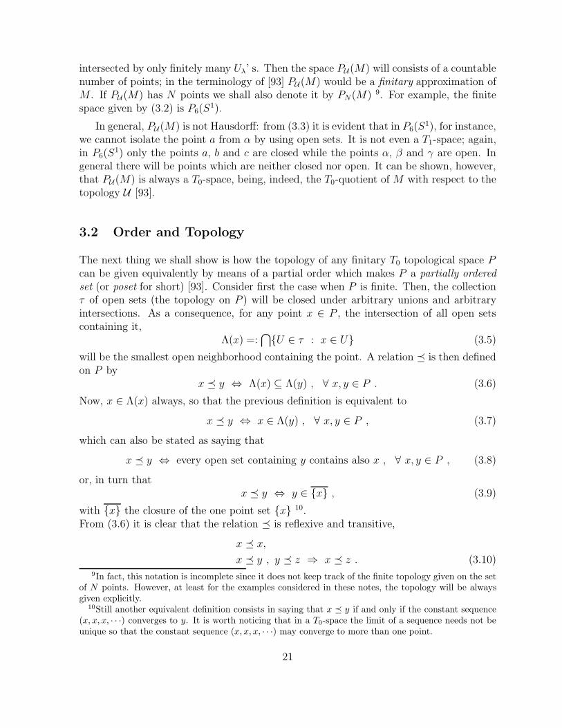
The next thing we shall show is how the topology of any finitary T0 topological space Pcan be given equivalently by means of a partial order which makes P a partially orderedset (or poset for short) [93]. Consider first the case when P is finite. Then, the collectionτ of open sets (the topology on P ) will be closed under arbitrary unions and arbitraryintersections. As a consequence, for any point x ∈ P , the intersection of all open setscontaining it,
Λ(x) =:⋂U ∈ τ : x ∈ U (3.5)
will be the smallest open neighborhood containing the point. A relation is then definedon P by
x y ⇔ Λ(x) ⊆ Λ(y) , ∀ x, y ∈ P . (3.6)
Now, x ∈ Λ(x) always, so that the previous definition is equivalent to
x y ⇔ x ∈ Λ(y) , ∀ x, y ∈ P , (3.7)
which can also be stated as saying that
x y ⇔ every open set containing y contains also x , ∀ x, y ∈ P , (3.8)
or, in turn thatx y ⇔ y ∈ x , (3.9)
with x the closure of the one point set x 10.From (3.6) it is clear that the relation is reflexive and transitive,
x x,
x y , y z ⇒ x z . (3.10)9In fact, this notation is incomplete since it does not keep track of the finite topology given on the set
of N points. However, at least for the examples considered in these notes, the topology will be alwaysgiven explicitly.
10Still another equivalent definition consists in saying that x y if and only if the constant sequence(x, x, x, · · ·) converges to y. It is worth noticing that in a T0-space the limit of a sequence needs not beunique so that the constant sequence (x, x, x, · · ·) may converge to more than one point.
21
Furthermore, being P a T0-space, for any two distinct points x, y ∈ P , there is at leastone open set containing x, say, and not y. This, together with (3.8), implies that therelation is antisymmetric as well,
x y , y x ⇒ x = y . (3.11)
Summing up, we get that a T0 topology on a finite space P determines a reflexive, an-tisymmetric and transitive relation, namely a partial order on P which makes the lattera partially ordered set (poset) . Conversely, given a partial order on the set P , oneproduces a topology on P by taking as a basis for it the finite collection of ‘open’ setsdefined as
Λ(x) =: y ∈ P : y x , ∀ x ∈ P. (3.12)
Thus, a subset W ⊂ P will be open if and only if is the union of sets of the form (3.12),namely, if and only if x ∈ W and y x ⇒ y ∈ W . Indeed, the smallest open setcontaining W is given by
Λ(W ) =⋃
x∈WΛ(x) , (3.13)
and W is open if and only if W = Λ(W ).The resulting topological space is clearly T0 by the antisymmetry of the order relation.
It is easy to express the closure operation in terms of the partial order. From (3.9),the closure V (x) = x, of the one point set x is given by
V (x) =: y ∈ P : x y , ∀ x ∈ P . (3.14)
A subset W ⊂ P will be closed if and only if x ∈ W and x y ⇒ y ∈ W . Indeed, theclosure of W is given by
V (W ) =⋃
x∈WV (x) , (3.15)
and W is closed if and only if W = V (W ).
If one relaxes the condition of finiteness of the space P , there is still an equivalencebetween topology and partial order for any T0 topological space which has the additionalproperty that every intersection of open sets is an open set (or equivalently, that everyunion of closet sets is a closed set), so that the sets (3.5) are all open and provide a basisfor the topology [2, 16]. This would be the case if P is a finitary approximation of a(locally compact) topological space M , obtained then from a locally finite covering of M11.
Given two posets P,Q, it is clear that a map f : P → Q will be continuous if andonly if it is order preserving, namely, if and only if x P y ⇒ f(x) Q f(y); indeed, fis continuous if and only if preserves convergence of sequences.In the sequel, x ≺ y will indicates that x precedes y while x 6= y.
11In fact, Sorkin [93] regards as finitary only those posets P for which the sets Λ(x) and V (x) definedin (3.13) and (3.14) respectively, are all finite. This would be the case if the poset is derived from alocally compact topological space with a locally finite covering consisting of bounded open sets.
22
A pictorial representation of the topology of a poset is obtained by constructing theassociated Hasse diagram: one arranges the points of the poset at different levels andconnects them by using the following rules :
1) if x ≺ y, then x is at a lower level than y;
2) if x ≺ y and there is no z such that x ≺ z ≺ y, then x is at the level immediatelybelow y and these two points are connected by a link.
s s
s s@@@@@@
x3 x4
x1 x2
s s
s s
s
s@@@@@@
@@@@@@
a
α
b
β
c
γ
Figure 1: The Hasse diagrams for P6(S1) and for P4(S
1).
The Fig. 1 shows the Hasse diagram for P6(S1) whose basis of open sets is in (3.3)
and for P4(S1). For the former, the partial order reads α ≺ a , α ≺ c , β ≺ a , β ≺
b , γ ≺ b , γ ≺ c. The latter is a four points approximation of S1 obtained from a coveringconsisting of two intersecting open sets. The partial order reads x1 ≺ x3 , x1 ≺ x4 , x2 ≺x3 , x2 ≺ x4 .In that Figure, (and in general, in any Hasse diagramindexHasse diagram) the smallestopen set containing any point x consists of all points which are below the given one x,and can be connected to it by a series of links. For instance, for P4(S
1) we get for theminimal open sets the following collection,
Now, the top two points are closed, the bottom two points are open and the intermediateones are neither closed nor open.
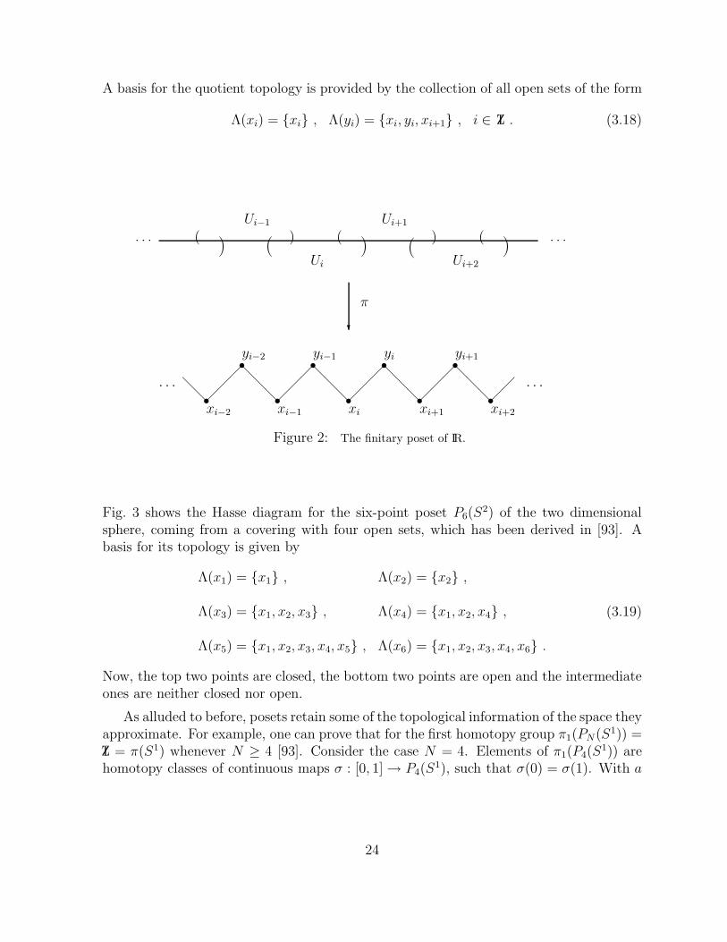
As alluded to before, posets retain some of the topological information of the space theyapproximate. For example, one can prove that for the first homotopy group π1(PN(S1)) =Z = π(S1) whenever N ≥ 4 [93]. Consider the case N = 4. Elements of π1(P4(S
any real number in the open interval ]0, 1[, consider the map
σ(t) =
x3 if t = 0x2 if 0 < t < ax4 if t = ax1 if a < t < 1x3 if t = 1
. (3.20)
Figure 4 shows this map for a = 1/2; the map can be seen to ‘winds once around’P4(S
1). Furthermore, the map σ in (3.20) is manifestly continuous, being constructed in
&%'$0, 1
σ-
s s
s s@@@@@@
6 6
@@R
0, 1 12
]12 , 1[ ]0, 12 [
Figure 4: A representative of the generator of the homotopy group π1(P4(S1)).
such a manner that closed (respectively open) points of P4(S1) are the image of closed
(respectively open) sets of the interval [0, 1] so that, automatically, the inverse image of anopen set in P4(S
1) is open in [0, 1]. A bit of extra analysis shows that σ is not contractibleto the constant map, any such contractible map being one that skips at least one of the
25
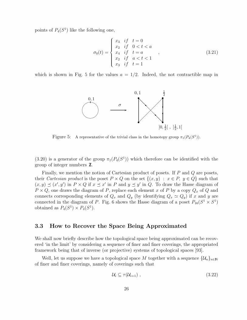
points of P4(S1) like the following one,
σ0(t) =
x3 if t = 0x2 if 0 < t < ax4 if t = ax2 if a < t < 1x3 if t = 1
, (3.21)
which is shown in Fig. 5 for the values a = 1/2. Indeed, the not contractible map in
&%'$0, 1
σ-
s s
s s@@@@@@
?
6
@@R
@@I
0, 1 12
]0, 12 [ , ]12 , 1[
Figure 5: A representative of the trivial class in the homotopy group π1(P4(S1)).
(3.20) is a generator of the group π1(P4(S1)) which therefore can be identified with the
group of integer numbers Z.
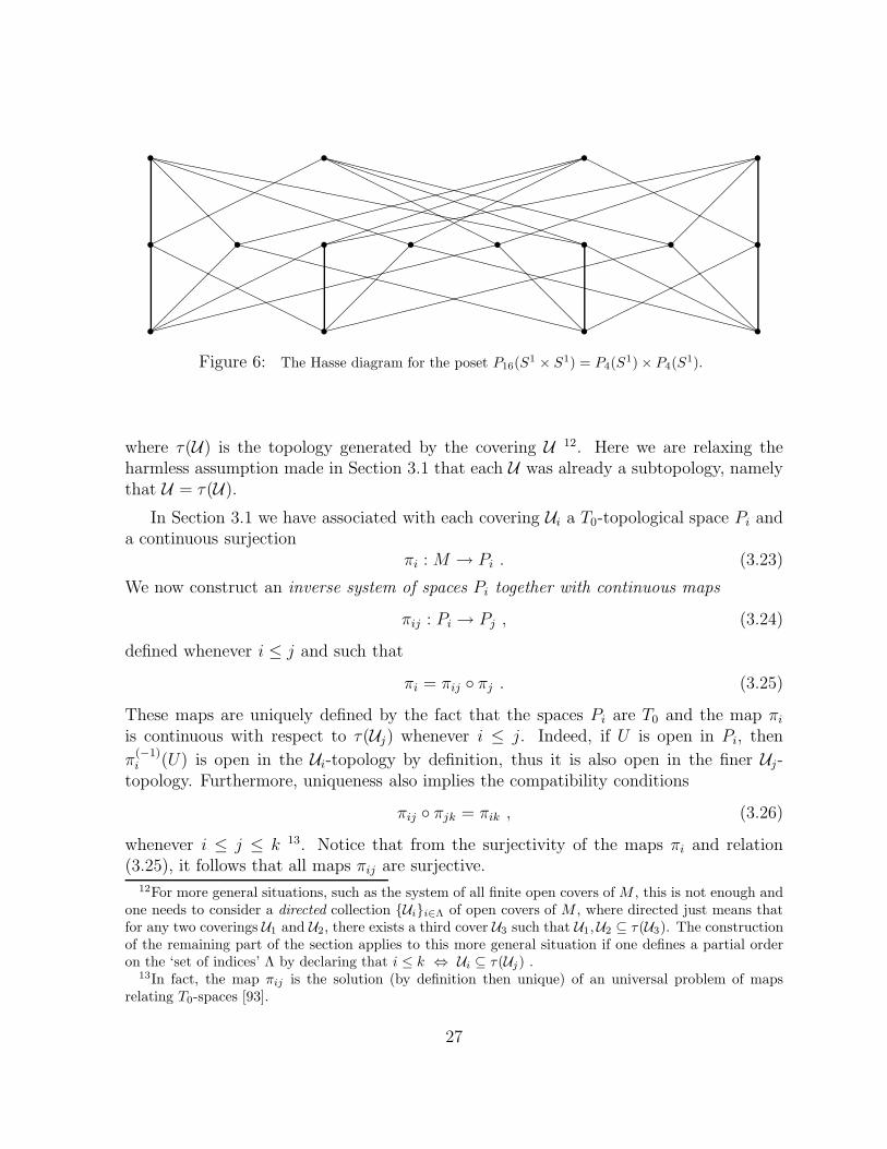
Finally, we mention the notion of Cartesian product of posets. If P and Q are posets,their Cartesian product is the poset P ×Q on the set (x, y) : x ∈ P, y ∈ Q such that(x, y) (x′, y′) in P × Q if x x′ in P and y y′ in Q. To draw the Hasse diagram ofP ×Q, one draws the diagram of P , replace each element x of P by a copy Qx of Q andconnects corresponding elements of Qx and Qy (by identifying Qx ≃ Qy) if x and y areconnected in the diagram of P . Fig. 6 shows the Hasse diagram of a poset P16(S
1 × S1)obtained as P4(S
1)× P4(S1).
3.3 How to Recover the Space Being Approximated
We shall now briefly describe how the topological space being approximated can be recov-ered ‘in the limit’ by considering a sequence of finer and finer coverings, the appropriatedframework being that of inverse (or projective) systems of topological spaces [93].
Well, let us suppose we have a topological space M together with a sequence Unn∈IN
of finer and finer coverings, namely of coverings such that
Ui ⊆ τ(Ui+1) , (3.22)
26
s ss s
s ss ss ss s
s ss s
@@@@@@
PPPPPPPPPPPPPPPPPP
``````````````````````````````
HHHHHHHHHHHH
HHHHHHHHHHHH
PPPPPPPPPPPPPPPPPP
XXXXXXXXXXXXXXXXXXXXXXXX
@@@@@@
HHHH
HHHH
HHHH
XXXXXX
XXXXXX
XXXXXX
XXXXXX
HHHH
HHHH
HHHH
@@@@@@
XXXXXX
XXXXXX
XXXXXX
XXXXXX
Figure 6: The Hasse diagram for the poset P16(S1 × S1) = P4(S
1)× P4(S1).
where τ(U) is the topology generated by the covering U 12. Here we are relaxing theharmless assumption made in Section 3.1 that each U was already a subtopology, namelythat U = τ(U).
In Section 3.1 we have associated with each covering Ui a T0-topological space Pi anda continuous surjection
πi : M → Pi . (3.23)
We now construct an inverse system of spaces Pi together with continuous maps
πij : Pi → Pj , (3.24)
defined whenever i ≤ j and such that
πi = πij πj . (3.25)
These maps are uniquely defined by the fact that the spaces Pi are T0 and the map πiis continuous with respect to τ(Uj) whenever i ≤ j. Indeed, if U is open in Pi, then
π(−1)i (U) is open in the Ui-topology by definition, thus it is also open in the finer Uj-
topology. Furthermore, uniqueness also implies the compatibility conditions
πij πjk = πik , (3.26)
whenever i ≤ j ≤ k 13. Notice that from the surjectivity of the maps πi and relation(3.25), it follows that all maps πij are surjective.
12For more general situations, such as the system of all finite open covers of M , this is not enough andone needs to consider a directed collection Uii∈Λ of open covers of M , where directed just means thatfor any two coverings U1 and U2, there exists a third cover U3 such that U1,U2 ⊆ τ(U3). The constructionof the remaining part of the section applies to this more general situation if one defines a partial orderon the ‘set of indices’ Λ by declaring that i ≤ k ⇔ Ui ⊆ τ(Uj) .
13In fact, the map πij is the solution (by definition then unique) of an universal problem of mapsrelating T0-spaces [93].
27
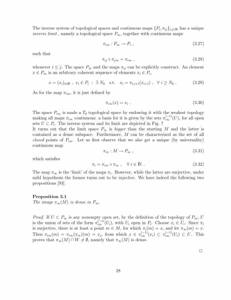
The inverse system of topological spaces and continuous maps Pi, πiji,j∈IN has a uniqueinverse limit , namely a topological space P∞, together with continuous maps
πi∞ : P∞ → Pi , (3.27)
such thatπij πj∞ = πi∞ , (3.28)
whenever i ≤ j. The space P∞ and the maps πij can be explicitly construct. An elementx ∈ P∞ is an arbitrary coherent sequence of elements xi ∈ Pi,
x = (xi)i∈IN , xi ∈ Pi : ∃ N0 s.t. xi = πi,i+1(xi+1) , ∀ i ≥ N0 . (3.29)
As for the map πi∞, it is just defined by
πi∞(x) = xi . (3.30)
The space Pi∞ is made a T0 topological space by endowing it with the weakest topologymaking all maps πi∞ continuous: a basis for it is given by the sets π
(−1)i∞ (U), for all open
sets U ⊂ Pi. The inverse system and its limit are depicted in Fig. 7It turns out that the limit space P∞ is bigger than the starting M and the latter iscontained as a dense subspace. Furthermore, M can be characterized as the set of allclosed points of Pi∞. Let us first observe that we also get a unique (by universality)continuous map
π∞ : M → P∞ , (3.31)
which satisfiesπi = πi∞ π∞ , ∀ i ∈ IN . (3.32)
The map π∞ is the ‘limit’ of the maps πi. However, while the latter are surjective, undermild hypothesis the former turns out to be injective. We have indeed the following twopropositions [93].
Proposition 3.1The image π∞(M) is dense in P∞.
Proof. If U ⊂ P∞ is any nonempty open set, by the definition of the topology of P∞, Uis the union of sets of the form π
(−1)i∞ (Ui), with Ui open in Pi. Choose xi ∈ Ui. Since πi
is surjective, there is at least a point m ∈ M , for which πi(m) = xi and let π∞(m) = x.
Then πi∞(m) = πi∞(π∞)(m) = xj, from which x ∈ π(−1)i∞ (xi) ⊂ π
(−1)i∞ (Ui) ⊂ U . This
proves that π∞(M) ∩W 6= ∅, namely that π∞(M) is dense.
2
28
M -
@@@@@@@@@@@@R
AAAAAAAAAAAAAAAAAAAAAAAAU
Pj
Pi
...
?
?
π∞
πij
πi
πj
πi∞
πj∞
P∞
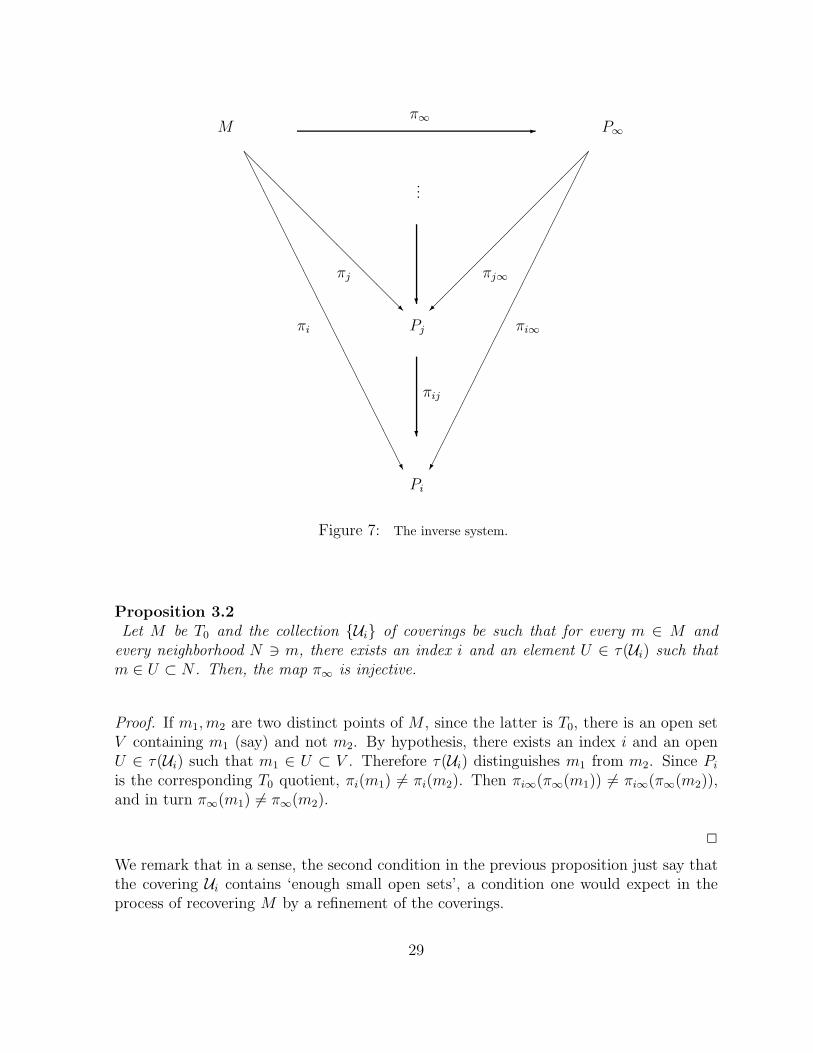
Figure 7: The inverse system.
Proposition 3.2Let M be T0 and the collection Ui of coverings be such that for every m ∈ M and
every neighborhood N ∋ m, there exists an index i and an element U ∈ τ(Ui) such thatm ∈ U ⊂ N . Then, the map π∞ is injective.
Proof. If m1, m2 are two distinct points of M , since the latter is T0, there is an open setV containing m1 (say) and not m2. By hypothesis, there exists an index i and an openU ∈ τ(Ui) such that m1 ∈ U ⊂ V . Therefore τ(Ui) distinguishes m1 from m2. Since Piis the corresponding T0 quotient, πi(m1) 6= πi(m2). Then πi∞(π∞(m1)) 6= πi∞(π∞(m2)),and in turn π∞(m1) 6= π∞(m2).
2
We remark that in a sense, the second condition in the previous proposition just say thatthe covering Ui contains ‘enough small open sets’, a condition one would expect in theprocess of recovering M by a refinement of the coverings.
29
As alluded to before, there is a nice characterization of the points of M (or betterof π∞(M)) as the set all all closed points of P∞. We have indeed a further Proposition,whose easy but long proof is given in [93],
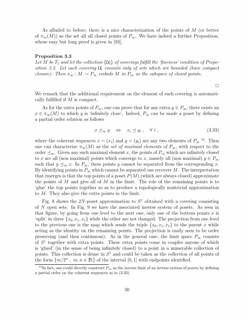
Proposition 3.3Let M be T1 and let the collection Ui of coverings fulfill the ‘fineness’ condition of Propo-sition 3.2. Let each covering Ui consists only of sets which are bounded (have compactclosure). Then π∞ : M → P∞ embeds M in P∞ as the subspace of closed points.
2
We remark that the additional requirement on the element of each covering is automati-cally fulfilled if M is compact.
As for the extra points of P∞, one can prove that for any extra y ∈ P∞, there exists anx ∈ π∞(M) to which y is ‘infinitely close’. Indeed, P∞ can be made a poset by defininga partial order relation as follows
x ∞ y ⇔ xi yi , ∀ i , (3.33)
where the coherent sequences x = (xi) and y = (yi) are any two elements of P∞14. Then
one can characterize π∞(M) as the set of maximal elements of P∞, with respect to theorder ∞. Given any such maximal element x, the points of P∞ which are infinitely closedto x are all (non maximal) points which converge to x, namely all (non maximal) y ∈ P∞such that y ∞ x. In P∞, these points y cannot be separated from the corresponding x.By identifying points in P∞ which cannot be separated one recovers M . The interpretationthat emerges is that the top points of a poset P (M) (which are always closed) approximatethe points of M and give all of M in the limit. The role of the remaining points is to‘glue’ the top points together so as to produce a topologically nontrivial approximationto M . They also give the extra points in the limit.
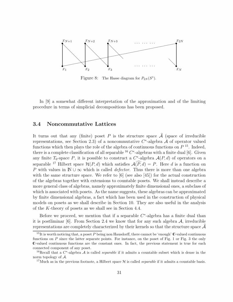
Fig. 8 shows the 2N -poset approximation to S1 obtained with a covering consistingof N open sets. In Fig. 9 we have the associated inverse system of posets. As seen inthat figure, by going from one level to the next one, only one of the bottom points x is‘split’ in three x0, x1, x1 while the other are not changed. The projection from one levelto the previous one is the map which sends the triple x0, x1, x1 to the parent x whileacting as the identity on the remaining points. The projection is easily seen to be orderpreserving (and then continuous). As in the general case, the limit space P∞ consistsof S1 together with extra points. These extra points come in couples anyone of whichis ‘glued’ (in the sense of being infinitely closed) to a point in a numerable collection ofpoints. This collection is dense in S1 and could be taken as the collection of all points ofthe form m/2n , m, n ∈ IN of the interval [0, 1] with endpoints identified.
14In fact, one could directly construct P∞ as the inverse limit of an inverse system of posets by defininga partial order on the coherent sequences as in (3.33).
30
s s s s
s s s s. . . . . . . . .
. . . . . . . . .
@
@@@@@
@@@@@@
@@@@
@@
xN+1 xN+2 xN+3 x2N
x1 x2 x3 xN
Figure 8: The Hasse diagram for P2N (S1).
In [9] a somewhat different interpretation of the approximation and of the limitingprocedure in terms of simplicial decompositions has been proposed.
3.4 Noncommutative Lattices
It turns out that any (finite) poset P is the structure space A (space of irreduciblerepresentations, see Section 2.3) of a noncommutative C∗-algebra A of operator valuedfunctions which then plays the role of the algebra of continuous functions on P 15. Indeed,there is a complete classification of all separable 16 C∗-algebras with a finite dual [6]. Givenany finite T0-space P , it is possible to construct a C∗-algebra A(P, d) of operators on a
separable 17 Hilbert space H(P, d) which satisfies A(P, d) = P . Here d is a function onP with values in IN ∪ ∞ which is called defector. Thus there is more than one algebrawith the same structure space. We refer to [6] (see also [45]) for the actual constructionof the algebras together with extensions to countable posets. We shall instead describe amore general class of algebras, namely approximately finite dimensional ones, a subclass ofwhich is associated with posets. As the name suggests, these algebras can be approximatedby finite dimensional algebras, a fact which has been used in the construction of physicalmodels on posets as we shall describe in Section 10. They are also useful in the analysisof the K-theory of posets as we shall see in Section 4.4.
Before we proceed, we mention that if a separable C∗-algebra has a finite dual thanit is postliminar [6]. From Section 2.4 we know that for any such algebra A, irreduciblerepresentations are completely characterized by their kernels so that the structure space A
15It is worth noticing that, a poset P being non Hausdorff, there cannot be ‘enough’ C-valued continuousfunctions on P since the latter separate points. For instance, on the poset of Fig. 1 or Fig. 3 the onlyC-valued continuous functions are the constant ones. In fact, the previous statement is true for eachconnected component of any poset.
16Recall that a C∗-algebra A is called separable if it admits a countable subset which is dense in thenorm topology of A.
17Much as in the previous footnote, a Hilbert space H is called separable if it admits a countable basis.
31
s s
s s@@@@@@
3 4
1 2
s s
s s
s
s@@@@@@
@@@@@@
3 20 4
1 21 22
s s
s s
s s
s s@@@@@@
@@@@@@
@@@@@@
10 3 20 4
12 11 21 22
...
?
?
π23
π12
Figure 9: The inverse system for S1.
32
is homeomorphic with the space PrimA of primitive ideals. As we shall see momentarily,the Jacobson topology on PrimA is equivalent to the partial order defined by inclusionof ideals. This fact in a sense ‘closes a circle’ making any poset, when thought of as thePrimA space of a noncommutative algebra, a truly noncommutative space or, rather, anoncommutative lattice.
3.4.1 The space PrimA as a Poset
Recall that in Section 2.3.1 we introduced the natural T0-topology (the Jacobson topology)on the space PrimA of primitive ideals of a noncommutative C∗-algebra A. In particular,from Prop. 2.6, we have that given any subset W of PrimA,
W is closed ⇔ I ∈W and I ⊆ J ⇒ J ∈W . (3.34)
Now, a partial order is naturally introduced on PrimA by inclusion,
I1 I2 ⇔ I1 ⊆ I2 , ∀ I1, I2 ∈ PrimA . (3.35)
From what we said after (3.14), given any subset W of the topological space (PrimA,),
W is closed ⇔ I ∈W and I J ⇒ J ∈W , (3.36)
which is just the partial order reading of (3.34). We infer that on PrimA the Jacobsontopology and the partial order topology can be identified.
3.4.2 AF-Algebras
In this section we shall describe approximately finite dimensional algebras using mainly[12]. A general algebra of this sort may have a rather complicated ideal structure anda complicated primitive ideal structure. As alluded to before, for applications to posetsonly a special subclass is selected.
Definition 3.1A C∗-algebra A is said to be approximately finite dimensional (AF) if there exists anincreasing sequence
A0I0→ A1
I1→ A2I2→ · · · In−1→ An
In→ · · · (3.37)
of finite dimensional C∗-subalgebras of A, such that A is the norm closure of⋃nAn , A =⋃
nAn. The maps In are injective ∗-morphisms.
3
33
The algebra A is the inductive (or direct) limit of the sequence An, Inn∈IN [102]. As aset,
⋃nAn is made of coherent sequences,
⋃
n
An = a = (an)n∈IN , an ∈ An | ∃N0 : an+1 = In(an) , ∀ n > N0. (3.38)
Now the sequence (||an||An)n∈IN is eventually decreasing since ||an+1|| ≤ ||an|| (the mapsIn are norm decreasing) and therefore convergent. One writes for the norm on A,
||(an)n∈IN|| = limn→∞ ||an||An . (3.39)
Since the maps In are injective, the expression (3.39) gives a true norm directly and notsimply a seminorm and there is no need to quotient out the zero norm elements. So, thealgebra A is the inductive (or direct) limit
⋃nAn of the sequence An, Inn∈IN [83, 102].
We shall assume that the algebra A has a unit II. If A and An are as before, then An+ CIIis clearly a finite dimensional C∗-subalgebras of A and An ⊂ An + CII ⊂ An+1 + CII. Wemay thus assume that each An contains the unit II of A and that the maps In are unital.
Example 3.1Let H be an infinite dimensional (separable) Hilbert space. The algebra
A = K(H) + CIIH , (3.40)
with K(H) the algebra of compact operators, is an AF-algebra [12]. The approximatingalgebras are given by
An = IMn(C)⊕ C , n > 0 , (3.41)
with embedding
IMn(C)⊕ C ∋ (Λ, λ) 7→(
Λ 00 λ
, λ
)∈ IMn+1(C)⊕ C . (3.42)
Indeed, let ξnn∈IN be an orthonormal basis in H and let Hn be the subspace generatedby the first n basis elements, ξ1, · · · , ξn. With Pn the orthogonal projection onto Hn,define
An = T ∈ B(H) : T (II−Pn) = (II− Pn)T ∈ C(II− Pn)≃ B(Hn)⊕ C ≃ IMn(C)⊕ C . (3.43)
Then An embeds in An+1 as in (3.42). Since each T ∈ An is a sum of a finite rankoperator and a multiple of the identity, one has that An ⊆ A = K(H) + CIIH and, inturn,
⋃nAn ⊆ A = K(H) + CIIH. Conversely, since finite rank operators are norm dense
in K(H), and finite linear combinations of strings ξ1, · · · , ξn are dense in H, one gets thatK(H) + CIIH ⊂
⋃nAn.
34
The algebra (3.40) has only two irreducible representations [6],
π1 : A −→ B(H) , a = (k + λIIH) 7→ π1(a) = a ,π2 : A −→ B(C) ≃ C , a = (k + λIIH) 7→ π2(a) = λ ,
(3.44)
with λ1, λ2 ∈ C and k ∈ K(H). The corresponding kernels are
I1 =: ker(π1) = 0 ,I2 =: ker(π2) = K(H) . (3.45)
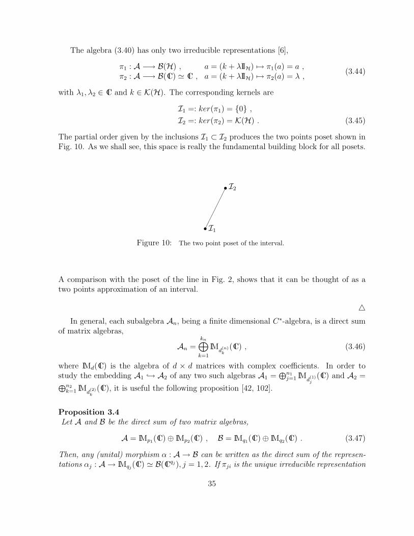
The partial order given by the inclusions I1 ⊂ I2 produces the two points poset shown inFig. 10. As we shall see, this space is really the fundamental building block for all posets.
s
s
I2
I1Figure 10: The two point poset of the interval.
A comparison with the poset of the line in Fig. 2, shows that it can be thought of as atwo points approximation of an interval.
In general, each subalgebra An, being a finite dimensional C∗-algebra, is a direct sum
of matrix algebras,
An =kn⊕
k=1
IMd(n)k
(C) , (3.46)
where IMd(C) is the algebra of d × d matrices with complex coefficients. In order tostudy the embedding A1 → A2 of any two such algebras A1 =
⊕n1j=1 IM
d(1)j
(C) and A2 =⊕n2k=1 IM
d(2)k
(C), it is useful the following proposition [42, 102].
Proposition 3.4Let A and B be the direct sum of two matrix algebras,
A = IMp1(C)⊕ IMp2(C) , B = IMq1(C)⊕ IMq2(C) . (3.47)
Then, any (unital) morphism α : A → B can be written as the direct sum of the represen-tations αj : A → IMqj(C) ≃ B(Cqj), j = 1, 2. If πji is the unique irreducible representation
35
of IMpi(C) in B(Cqj), then αj breaks into a direct sum of the πji with multiplicity Nji, the
latter being non-negative integers.
Proof. This proposition just says that, by suppressing the symbols πji, and modulo achange of basis, the morphism α : A → B is of the form
A⊕
B 7→ A⊕ · · · ⊕ A︸ ︷︷ ︸N11
⊕B ⊕ · · · ⊕ B︸ ︷︷ ︸N12
⊕A⊕ · · · ⊕A︸ ︷︷ ︸
N21
⊕B ⊕ · · · ⊕ B︸ ︷︷ ︸N22
, (3.48)
with A⊕B ∈ A. Moreover, the dimensions (p1, p2) and (q1, q2) are related by
N11p1 +N12p2 = q1 ,
N21p1 +N22p2 = q2 . (3.49)
2
Given a unital embedding A1 → A2 of the algebras A1 =⊕n1j=1 IM
d(1)j
(C) and A2 =⊕n2k=1 IM
d(2)k
(C), by using Proposition 3.4 one can always choose suitable bases in A1 and
A2 in such a manner to identify A1 with a subalgebra of A2 of the following form
A1 ≃n2⊕
k=1
n1⊕
j=1
NkjIMd(1)j
(C)
. (3.50)
Here, with any two nonnegative integers p, q, the symbol pIMq(C) stands for
pIMq(C) ≃ IMq(C)⊗C IIp , (3.51)
and one identifies⊕n1j=1NkjIMd
(1)j
(C) with a subalgebra of IMd(2)k
(C). The nonnegative
integers Nkj satisfies the condition
n1∑
j=1
Nkjd(1)j = d
(2)k . (3.52)
One says that the algebra IMd(1)j
(C) is partially embedded indexpartial embedding in
IMd(2)k
(C) with multiplicity Nkj. A useful way to represent the algebras A1, A2 and the
embedding A1 → A2 is by means of a diagram, the Bratteli diagram [12], which can be
constructed out of the dimensions d(1)j , j = 1, . . . , n1 and d
(2)k , k = 1, . . . , n2, of the
diagonal blocks of the two algebras and of the numbers Nkj that describe the partial em-beddings. One draws two horizontal rows of vertices, the top (bottom) ones representingA1 (A2) and consisting of n1 (n2) vertices, one for each block, labeled by the corresponding
dimensions d(1)1 , . . . , d(1)
n1(d
(2)1 , . . . , d(2)
n2). Then, for each j = 1, . . . , n1 and k = 1, . . . , n2,
one has a relation d(1)j ցNkj d
(2)k to denote the fact that IM
d(1)j
(C) is embedded in IMd(2)k
(C)
with multiplicity Nkj.
36
For any AF-algebra A one repeats the procedure for each level so obtaining a semi-infinite diagram denoted by D(A) which completely defines A up to isomorphism. Thediagram D(A) depends not only on A but also on the particular sequence Ann∈IN whichgenerate A. However, one can obtain an algorithm which allows one to construct froma given diagram all diagrams which define AF-algebras which are isomorphic with theoriginal one [12]. The problem of identifying the limit algebra or of determining whetheror not two such limits are isomorphic can be very subtle. Elliot [43] has devised a completeinvariant for AF-algebras in terms of the corresponding K theory which distinguishesamong them (see also [42]). We shall elaborate a bit on this in Section 4.4. It is worthremarking that the isomorphism class on an AF-algebra
⋃nAn depends not only on the
An but also on the way they are embedded into each other.
Any AF-algebra is clearly separable but the converse is not true. Indeed, one can provethat a separable C∗-algebra A is an AF-algebra if and only if and it has the followingapproximation property: for each finite set a1, . . . , an of elements of A and ε > 0,there exists a finite dimensional C∗-algebra B ⊆ A and elements b1, . . . , bn ∈ B such that||ak − bk|| < ε , k = 1, . . . , n .
Given a set D of ordered pairs (n, k), k = 1, · · · , kn , n = 0, 1, · · ·, with k0 = 1, and asequence ցpp=0,1,··· of relations on D, the latter is the diagram D(A) of an AF-algebraswhen the following conditions are satisfied,
(i) If (n, k), (m, q) ∈ D and m = n + 1, there exists one and only one nonnegative (orequivalently, at most a positive) integer p such that (n, k)ցp (n+ 1, q).
(ii) If m 6= n+ 1 not such integer exists.
(iii) If (n, k) ∈ D there exists q ∈ 1, · · · , nn+1 and a nonnegative integer p such that(n, k)ցp (n+ 1, q).
(iv) If (n, k) ∈ D and n > 0, there exists q ∈ 1, · · · , nn−1 and a nonnegative integer psuch that (n− 1, q)ցp (n, k).
It is easy to see that the diagram of a given AF-algebra satisfies the previous condi-tions. Conversely, if the set D of ordered pairs satisfies these properties, one constructsby induction a sequence of finite dimensional C∗-algebras Ann∈IN and of injective mor-phisms In : An → An+1 in such a manner that the inductive limit An, Inn∈IN will havediagram D. Explicitly, one defines
An =⊕
k;(n,k)∈DIM
d(n)k
(C) =kn⊕
k=1
IMd(n)k
(C) , (3.53)
and morphisms
In :jn⊕
j=1
IMd(n)j
(C) −→kn+1⊕
k=1
IMd(n+1)k
(C) ,
A1 ⊕ · · · ⊕ Ajn 7→ (⊕jnj=1N1jAj)⊕· · ·
⊕(⊕jnj=1Nkn+1jAj) , (3.54)
37
where the integers Nkj are such that (n, j)ցNkj (n+1, k) and we have used the notation
(3.51). Notice that the dimension d(n+1)k of the factor IM
d(n+1)k
(C) is not arbitrary but it
is determined by a relation like (3.52), namely d(n+1)k =
∑jnj=1Nkjd
(n)j .
Example 3.2An AF-algebra A is abelian if and only if all factors IM
d(n)k
(C) are one dimensional,
IMd(n)k
(C) ≃ C. Thus the corresponding diagram D has the property that for each (n, k) ∈D, n > 0, there is exactly one (n− 1, j) ∈ D such that (n− 1, j)ց1 (n, k).
There is a very nice characterization of commutative AF-algebras and of their primitivespectra [13].
Proposition 3.5Let A be a commutative C∗-algebra with unit I. Then the following statements are equiv-alent.
(i) The algebra A is AF.
(ii) The algebra A is generated in the norm topology by a sequence of projectors Pi,with I0 = I.
(iii) The space PrimA is a second-countable, totally disconnected, compact Hausdorffspace 18.
Proof. The equivalence of (i) and (ii) is clear. To prove that (iii) implies (ii), let Xbe a second-countable, totally disconnected, compact Hausdorff space. Then X has acountable basis Xn of open-closed sets. Let Pn be the characteristic function of Xn.The ∗-algebra generated by the projector Pn is dense in C(X): since PrimC(X) = X,(iii) implies (ii). The converse, that (ii) implies (iii), follows from the fact that projectorsin a commutative C∗-algebra correspond to open-closed subset in its primitive spaces.
2
Example 3.3Let us consider the subalgebra A of the algebra B(H) of bounded operators on an infinitedimensional (separable) Hilbert space H = H1 ⊕H2, given in the following manner. Let
18We recall that a topological space is called totally disconnected if the connected component of eachpoint consists only of the point itself. Also, a topological space is called second-countable is it admits acountable basis of open sets.
38
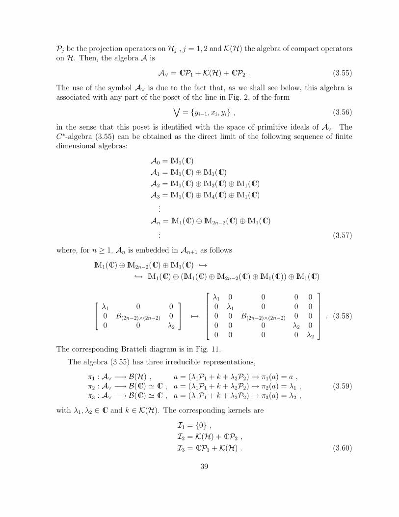
Pj be the projection operators onHj , j = 1, 2 and K(H) the algebra of compact operatorson H. Then, the algebra A is
A∨ = CP1 +K(H) + CP2 . (3.55)
The use of the symbol A∨ is due to the fact that, as we shall see below, this algebra isassociated with any part of the poset of the line in Fig. 2, of the form
∨= yi−1, xi, yi , (3.56)
in the sense that this poset is identified with the space of primitive ideals of A∨. TheC∗-algebra (3.55) can be obtained as the direct limit of the following sequence of finitedimensional algebras:
A0 = IM1(C)
A1 = IM1(C)⊕ IM1(C)
A2 = IM1(C)⊕ IM2(C)⊕ IM1(C)
A3 = IM1(C)⊕ IM4(C)⊕ IM1(C)...
An = IM1(C)⊕ IM2n−2(C)⊕ IM1(C)... (3.57)
where, for n ≥ 1, An is embedded in An+1 as follows
The algebra (3.55) has three irreducible representations,
π1 : A∨ −→ B(H) , a = (λ1P1 + k + λ2P2) 7→ π1(a) = a ,π2 : A∨ −→ B(C) ≃ C , a = (λ1P1 + k + λ2P2) 7→ π2(a) = λ1 ,π3 : A∨ −→ B(C) ≃ C , a = (λ1P1 + k + λ2P2) 7→ π3(a) = λ2 ,
(3.59)
with λ1, λ2 ∈ C and k ∈ K(H). The corresponding kernels are
I1 = 0 ,I2 = K(H) + CP2 ,
I3 = CP1 +K(H) . (3.60)
39
ssss
s
sss
ssss
@@@
@@@
@@@
@@@
@
1
1
1
1
1
1
1
1
1
2
4
6
......
Figure 11: The Bratteli diagram of the algebra A∨. The labels indicate the dimension of the corre-
sponding matrix algebras.
The partial order given by the inclusions I1 ⊂ I2 and I1 ⊂ I3 (which, as shown inSection 3.4.1 is an equivalent way to provide the Jacobson topology) produces a topologicalspace PrimA∨ which is just the
∨poset in (3.56).
3.4.3 From Bratteli Diagrams to Noncommutative Lattices
From the Bratteli diagram of an AF-algebra A one can also obtain the (norm closedtwo-sided) ideals of the latter and determine which ones are primitive. On the set of suchideals the topology is then given by constructing a poset whose partial order is providedby inclusion of ideals. Therefore, both Prim(A) and its topology can be determined fromthe Bratteli diagram of A. This is possible thanks to the following results by Bratteli[12].
Proposition 3.6Let A =
⋃n Un be any AF-algebra with associated Bratteli diagram D(A). Let I be an
ideal of A. Then I has the form
I =∞⋃
n=1
⊕k;(n,k)∈ΛIIM
d(n)k
(C) (3.61)
with the subset ΛI ⊂ D(A) satisfying the following two properties:
40
i) if (n, k) ∈ ΛI and (n, k)ցp (n + 1, j) , p > 0, then (n+ 1, j) belongs to ΛI ;
ii) if all factors (n+ 1, j) , j = 1, . . . , nn+1, in which (n, k) is partially embedded belongto ΛI, then (n, k) belongs to ΛI .
Conversely, if Λ ⊂ D(A) satisfies properties (i) and (ii) above, then the subset IΛ ofA defined by (3.61) (with Λ substituted for ΛI) is an ideal in A such that I ⋂An =⊕k;(n,k)∈ΛI
IMd(n)k
(C).
2
Proposition 3.7Let A =
⋃n Un, let I be an ideal of A and let ΛI ⊂ D(A) be the associated subdiagram.
Then the following conditions are equivalent 19.
(i) The ideal I is primitive.
(ii) There does not exist two ideals I1, I2 ∈ A such that I1 6= I 6= I2 and I = I1 ∩ I2.
(iii) If (n, k), (m, q) /∈ ΛI, there exists an integer p ≥ n,m and a couple (p, r) /∈ ΛI suchthat IM
d(n)k
(C) and IMd(m)q
(C) are both partially embedded in IMd(p)r
(C) (equivalently,
there are two sequences along the diagram D(A) starting at the points (n, k) and(m, q) both ending at the point (p, r)).
2
We recall that the whole A is an ideal which, by definition, is not primitive since the trivialrepresentation A → 0 is not irreducible. Furthermore, the ideal 0 ⊂ A is primitive ifand only if A is primitive, namely it has an irreducible faithful representation. This factcan also be inferred from the Bratteli diagram. Now, the ideal 0, being representedby the element 0 ∈ An at each level 20, is not associated with any subdiagram of D(A).Therefore, to check if 0 is primitive we have the following corollary of Proposition 3.7.
Proposition 3.8Let A =
⋃n Un. Then the following conditions are equivalent.
(i) The algebra A is primitive (namely the ideal 0 is primitive).
(ii) There does not exist two ideals in A different from 0 whose intersection is 0.
(iii) If (n, k), (m, q) ∈ D(A), there exists an integer p ≥ n,m and a couple (p, r) ∈D(A) such that IM
d(n)k
(C) and IMd(m)q
(C) are both partially embedded in IMd(p)r
(C)
(equivalently, any two points of the diagram D(A) can be connected to a single pointat a later level of the diagram).
19In fact, the equivalence of (i) and (ii) is true for any separable C∗-algebra [34]20In fact one could think of Λ0 as being the empty set.
41
⋆
⋆
⋆
⋆
⋆
⋆
⋆
@@@
@@@
@@@
@@@
@
⋆
⋆
⋆
⋆
⋆
⋆
⋆
@@@
@@@
@@@
@@@
@
⋆
⋆
⋆
@@@
@@@
@@@
@@@
@
(a) (b) (c)
I2 I3 IK
......
......
......
Figure 12: The three ideals of the algebra A∨.
2
For instance, from the diagram of Fig. 11 we infer that the corresponding algebra isprimitive, namely the ideal 0 is primitive.
Example 3.4As a simple example, consider the diagram of Fig. 11. The corresponding AF-algebra A∨in (3.55) contains only three nontrivial ideals, whose diagrammatic representation is inFig. 12. In this pictures the points belonging to the same ideal are marked with a “⋆”. Itis not difficult to check that only I2 and I3 are primitive ideals, since IK does not satisfyproperty (iii) above. Now I1 = 0 is an ideal which clearly belongs to both I2 and I3 sothat Prim(A) is any
∨part of Fig. 2 of the form
∨= yi−1, xi, yi. From the diagram
of Figure 12 one immediately obtains
I2 = CIIH +K(H) ,
I1 = CIIH +K(H) , (3.62)
H being an infinite dimensional Hilbert space. Thus, I2 and I3 can be identified with thecorresponding ideals of A∨ given in (3.60). As for IK, from Figure 12 one gets IK = K(H)which is not a primitive ideal of A∨.
42
3.4.4 From Noncommutative Lattices to Bratteli Diagrams
Bratteli [13] has also a reverse procedure which allows one to construct an AF-algebra(or rather its Bratteli diagram D(A)) whose primitive ideal space is a given (finitary,noncommutative) lattice P . We shall briefly describe this procedure while referring to[44, 45] for more details and several examples.
Proposition 3.9Let P be a topological space with the following properties,
(i) The space P is T0.
(ii) If F ⊂ P is a closed set which is not the union of two proper closed subset, then Fis the closure of a one-point set.
(iii) The space P contains at most a countable number of closed sets.
(iv) If Fnn is a decreasing (Fn+1 ⊂ Fn) sequence of closed subsets of P , then⋂n Fn is
an element in Fnn.
Then, there exists an AF algebra A whose primitive space PrimA is homeomorphic to P .
Proof. The proof consists in constructing explicitly the Bratteli diagram D(A) of thealgebra A. We shall sketch the main passages while referring to [13] for more details.
Let K0, K1, K2, . . . be the collection of all closed sets in the lattice P , with K0 = P .
Consider the subcollection Kn = K0, K1, . . . , Kn and let K′n be the smallest collec-
tion of (closed) sets in P containing Kn which is closed under union and intersection.
Consider the algebra of sets 21 generated by the collection Kn. Then, the minimal setsYn = Yn(1), Yn(2), . . . , Yn(kn) of the algebra form a partition of P .
Let Fn(j) be the smallest set in the subcollection K′n which contains Yn(j). Define
Fn = Fn(1), Fn(2), . . . , Fn(kn).
As a consequence of the assumptions in the propositions one has that
Yn(k) ⊆ Fn(k) , (3.63)
21We recall that a non empty collection R of subsets of a set X is called an algebra if R is closedunder the operation of union, namely E, F ∈ R⇒ E ∪ F ∈ R and the operation of complement, namelyE ∈ R⇒ Ec =: X \ E ∈ R.
43
⋃
k
Yn(k) = P , (3.64)
⋃
k
Fn(k) = P , (3.65)
Yn(k) = Fn(k) \⋃
p 6=kFn(p) | Fn(p) ⊂ Fn(k) , (3.66)
Fn(k) =⋃
p
Fn+1(p) | Fn+1(p) ⊆ Fn(k) , (3.67)
If F ⊂ P is closed , ∃ n ≥ 0 , s.t. Fn(k) =⋃
p
Fn(p) | Fn(p) ⊆ F . (3.68)
The diagram D(A) is constructed as follows.
1. The n-th level of D(A) has kn points, one for each set Yn(k), k = 1, · · · , kn.Thus D(A) is the set of all ordered pairs (n, k) , k = 1, . . . , kn , n = 0, 1, . . ..
2. The point corresponding to Yn(k) at the level n of the diagram is linked to the pointcorresponding to Yn+1(j) at the level n+ 1, if and only if Yn(k)∩ Fn+1(j) 6= ∅. Themultiplicity of the embedding is always 1.Thus, the partial embeddings of the diagram are given by
(n, k) ցp (n+ 1, j) , with
p = 1 if Yn(k) ∩ Fn+1(j) 6= ∅ ,p = 0 otherwise . (3.69)
That the diagram D(A) is really the diagram of an AF algebra A, namely that conditions(i)− (iv) of page 37 are satisfied, follows from conditions (3.63)-(3.68) above.
Before we proceed, recall from Proposition (2.5) that there is a bijective correspondencebetween ideals in a C∗-algebra and closed sets in PrimA, the correspondence being givenby (2.33). We shall then construct a similar correspondence between closed subsets F ⊆ Pand the ideals IF in the AF-algebra A with subdiagram ΛF ⊆ D(A). Given then, a closedsubset F ⊆ P , from (3.68), there exists an m such that F ⊆ K′
m. Define
(ΛF )n = (n, k) | n ≥ m , Yn(k) ∩ F = ∅ . (3.70)
By using (3.66) one proves that conditions (i) and (ii) of Proposition 3.6 are satisfied.As a consequence, if ΛF is the smallest subdiagram corresponding to an ideal IF , namelysatisfying conditions (i) and (ii) of Proposition 3.6, which also contains (ΛF )n, one hasthat
(ΛF )n = ΛF
⋂(n, k) | (n, k) ∈ D(A), n ≥ m , (3.71)
which, in turn, implies that the mapping F 7→ ΛF ↔ IF is injective.To show surjectivity, let I be an ideal in A with associated subdiagram ΛI . Define
Then Fnn is a decreasing sequence of closet sets in P . By assumption (iv), there existsan m such that Fm =
⋂n Fn. By defining F = Fn, one has Fn = F for n ≥ m and
ΛI⋂(n, k) | n ≥ m =: (ΛF )m . (3.73)
Thus, ΛI = ΛF and the mapping F 7→ IF is surjective.Finally, from definition it follows that
F1 ⊆ F2 ⇐⇒ IF1 ⊇ IF2 . (3.74)
For any point x ∈ P , the closure x is not the union of two proper closed subset. From(3.74), the corresponding ideal Ix is not the intersection of two ideals different from
itself, thus it is primitive (see Proposition 3.7). Conversely, if IF is primitive, it is notthe intersection of two ideals different from itself, thus from (3.74) F is not the union oftwo proper closed subsets, and from assumption (ii), it is the closure of a one-point set.We have then proved that the ideal IF is primitive if and only if F is the closure of aone-point set.By taking into account the bijection between closed sets of the space P and ideals of thealgebra A and the corresponding bijection between of closed sets of the space PrimA andideals of the algebra A, we see that the bijection between P and PrimA which associatesto any point of P the corresponding primitive ideal, is a homeomorphism.
2
We know that different algebras could give the same space of primitive ideals (see thenotion of strong Morita equivalence in Section D). It may happen that by changing theorder in which the closed sets of P are taken in the construction of the previous propo-sition, one produces different algebras, all of which having the same space of primitiveideals though, so all producing spaces which are homeomorphic to the starting P (anytwo of these spaces being, a fortiori, homeomorphic).
Example 3.5As a simple example, consider again the lattice,
∨has only a finite number of points (three) and hence a finite number of closed
sets (four), the partition of∨
repeats itself after the third level. Fig. 13 shows thecorresponding diagram, obtained through rules (1.) and (2.) in Proposition 3.9 above. Byusing the fact that the first matrix algebra A0 is C and the fact that all the embeddingshave multiplicity one, the diagram of Fig. 13 is seen to coincide with the diagram ofFig. 11. As we have said previously, the latter corresponds to the AF-algebra A∨ =CP1 +K(H) + CP2 , H = H1 ⊕H2.
Example 3.6Another interesting example is provided by the lattice P4(S
1) for the one-dimensional
46
sphere in Fig. 1. This topological space contains six closed sets:
Since there is a finite number of points (four) and hence a finite number of closed sets (six),the partition of P4(S
1) repeats itself after the fourth level. The corresponding Brattelidiagram is in Fig. 14. The ideal 0 is not primitive. The algebra is given by
A0 = IM1(C)
A1 = IM1(C)⊕ IM1(C)
A2 = IM1(C)⊕ IM2(C)⊕ IM1(C)
A3 = IM1(C)⊕ IM4(C)⊕ IM2(C)⊕ IM1(C)
A4 = IM1(C)⊕ IM6(C)⊕ IM4(C)⊕ IM1(C)...
47
ssssss
sssss
sss s
sss
@@@
@@@
PPPPPPPPP@@@
@@@
@@@
HHHHHHHHHHHHHHHHHH@HH
...
Figure 14: The Bratteli diagram for the circle poset P4(S1) .
An = IM1(C)⊕ IM2n−2(C)⊕ IM2n−4(C)⊕ IM1(C)... (3.79)
where, for n > 2, An is embedded in An+1 as follows
λ1
BC
λ2
7→
λ1
λ1 0 00 B 00 0 λ2
λ1 0 00 C 00 0 λ2
λ2
, (3.80)
with B ∈ IM2n−2(C) and C ∈ IM2n−4(C); elements which are not shown are equal to zero.The algebra limit AP4(S1) can be realized explicitly as a subalgebra of bounded operatorson an infinite dimensional Hilbert space H naturally associated with the poset P4(S
1).Firstly, to any link (xi, xj), xi ≻ xj , of the latter one associates an Hilbert space Hij ; forthe case at hand, one has four Hilbert spaces, H31,H32,H41,H42. Then, since all links areat the same level, H is just given by the direct sum
Here K denotes compact operators and P orthogonal projection. The algebra (3.82) hasfour irreducible representations. Any element a ∈ AP4(S1) is of the form
a = λP3,12 + k34,1 + k34,2 + µP4,12 , (3.83)
with λ, µ ∈ C, k34,1 ∈ KH31⊕H41 and k34,2 ∈ KH32⊕H42 . The representations are thefollowing ones,
π1 : AP4(S1) −→ B(H) , a 7→ π1(a) = λP3,12 + k34,1 + µP4,12 ,π2 : AP4(S1) −→ B(H) , a 7→ π2(a) = λP3,12 + k34,2 + µP4,12 ,π3 : AP4(S1) −→ B(C) ≃ C , a 7→ π3(a) = λ ,π4 : AP4(S1) −→ B(C) ≃ C , a 7→ π4(a) = µ .
(3.84)
The corresponding kernels are
I1 = KH32⊕H42 ,
I2 = KH31⊕H41 ,
I3 = KH31⊕H41 +KH32⊕H42 + CPH41⊕H42 ,
I4 = CPH31⊕H32 +KH31⊕H41 + KH32⊕H42 . (3.85)
The partial order given by the inclusions I1 ⊂ I3, I1 ⊂ I4 and I2 ⊂ I3, I2 ⊂ I4 producesa topological space PrimAP4(S1) which is just the circle poset in Fig. 1.
Example 3.7We shall now give an example of a three-level poset. It would correspond to an approxi-mation of a two dimensional topological space (or a portion thereof).
This topological space, shown in Fig. 15, contains five closed sets:
Since there is a finite number of points (four) and hence a finite number of closed sets(five), the partition of the poset is the same after the fourth level. The corresponding
50
ssssss
sssss
sss s
sss
@@@
@@@
PPPPPPPPP@@@
HHHHHH@@@
HHHHHH
@@@
HHHHHH@HH
...
Figure 16: The Bratteli diagram for the poset Y of previous Figure.
Bratteli diagram is in Fig. 16. The ideal 0 is primitive. The corresponding algebra isgiven by
A0 = IM1(C)
A1 = IM1(C)⊕ IM1(C)
A2 = IM1(C)⊕ IM2(C)⊕ IM1(C)
A3 = IM1(C)⊕ IM4(C)⊕ IM2(C)⊕ IM1(C)
A4 = IM1(C)⊕ IM8(C)⊕ IM4(C)⊕ IM1(C)...
An = IM1(C)⊕ IMn2−3n+4(C)⊕ IM2n−4(C)⊕ IM1(C)... (3.88)
51
where, for n > 2, An is embedded in An+1 as follows
λ1
BC
λ2
7→
λ1
λ1 0 0 00 B 0 00 0 C 00 0 0 λ2
λ1 0 00 C 00 0 λ2
λ2
, (3.89)
with B ∈ IMn2−3n+4(C) and C ∈ IM2n−4(C); elements which are not shown are equal tozero. Again, the algebra limit AY can be given as a subalgebra of bounded operatorson a Hilbert space H. The Hilbert spaces associated with the links of the poset will beH32,H42,H21. The difference with the previous example is that now there are links atdifferent levels. On passing from a level to the next (or previous one) one introducestensor products. The Hilbert space H is given by
H = H32 ⊗H21 ⊕H42 ⊗H21 ≃ (H32 ⊕H42)⊗H21 (3.90)
The algebra AY is then given by [45],
AY = CPH32⊗H21 +KH32⊕H42 ⊗PH21 +K(H32⊕H42)⊗H21 + CPH42⊗H21 . (3.91)
Here K denotes compact operators and P orthogonal projection. This algebra has fourirreducible representations. Any element of it is of the form
a = λP321 + k34,2 ⊗ P21 + k34,21 + µP421 , (3.92)
with λ, µ ∈ C, k34,2 ∈ KH32⊕H42 and k34,21 ∈ K(H32⊕H42)⊗H21. The representations are the
following ones,
π1 : AY −→ B(H) , a 7→ π1(a) = λP321 + k34,2 ⊗ P21 + k34,21 + µP421 ,π2 : AY −→ B(H) , a 7→ π2(a) = λP321 + k34,2 ⊗ P21 + µP421 ,π3 : AY −→ B(C) ≃ C , a 7→ π3(a) = λ ,π4 : AY −→ B(C) ≃ C , a 7→ π4(a) = µ .
The partial order given by the inclusions I1 ⊂ I2 ⊂ I3 and I1 ⊂ I2 ⊂ I4 produces atopological space PrimAY which is just the poset of Fig. (15).
52
In fact, by looking at the previous examples a bit more carefully one can infer the
algorithm by which one goes from a (finite) poset P to the corresponding Bratteli diagramD(AP ). Let (x1, · · · , xN ) be the points of P and for k = 1, · · · , N , let Sk =: xk be thesmallest closet subset of P containing the point xj . Then, the Bratteli diagram repeatsitself after the level N and the partition Yn(k) of Proposition 3.9 is just given by
Yn(k) = Yn+1(k) = xk , k = 1, . . . , N, ∀ n ≥ N . (3.95)
As for the associated Fn(k), from the level N + 1 on, they are given by the Sk,
Fn(k) = Fn+1(k) = Sk , k = 1, . . . , N, ∀ n ≥ N + 1 . (3.96)
In the diagram D(AP ), for any n ≥ N , (n, k) ց (n + 1, j) if and only if xk⋂Sj 6= ∅,
namely if and only if xk ∈ Sj .We also sketch the algorithm to construct the algebra limit AP determined by the Brattelidiagram D(AP ) 22 [6, 45]. The idea is to associate to the poset P an infinite dimensionalseparable Hilbert space H(P ) out of tensor products and direct sums of infinite dimen-sional (separable) Hilbert spaces Hij associated with each link (xi, xj), xi ≻ xj , in theposet 23. Then for each point x ∈ P there is a subspace H(x) ⊂ H(P ) and an algebraB(x) of bounded operators acting on H(x). The algebra AP is the one generated by allof the B(x) as x varies in P . In fact, the algebra B(x) can be made to act on the whole ofH(P ) by defining its action on the complement of H(x) to be zero. Consider any maximalchain Cα in P : Cα = xa, . . . , x2, x1 | xj ≻ xj−1 for any maximal point xα. To this chainone associates the Hilbert space
H(Cα) = Hα,α−1 ⊗ · · · ⊗ H3,2 ⊗H2,1 . (3.97)
By taking the direct sum over all maximal chains, one gets the Hilbert space H(P ),
H(P ) =⊕
α
H(Cα) . (3.98)
The subspace H(x) ⊂ H(P ) associated with any point x ∈ P is constructed in a similarmanner by restricting the sum to all maximal chains containing the point x. It can besplit in two parts,
H(x) = H(x)u ⊗H(x)d , (3.99)
with,
H(x)u = H(P ux ) , P u
x = y ∈ P | y x ,H(x)d = H(P d
x ) , P dx = y ∈ P | y x . (3.100)
22This algebra is really defined only modulo Morita equivalence.23The Hilbert spaces could be taken to be all the same. The label is there just to distinguish among
them.
53
Here H(P ux ) and H(P d
x ) are constructed as in (3.98); also, H(x)u = C if x is a maximalpoint and H(x)d = C if x is a minimal point. Consider now the algebra B(x) of boundedoperators on H(x) given by
As before, K denotes compact operators and P orthogonal projection. We see that B(x)acts by compact operators on the Hilbert space H(x)u determined by the points whichfollow x and by multiplies of the identity on the Hilbert space H(x)d determined by thepoints which precede x. These algebras satisfy the rules: B(x)B(y) ⊂ B(x) if x y andB(x)B(y) = 0 if x and y are not comparable. As already mentioned, the algebra A(P ) ofthe poset P is the algebra of bounded operators on H(P ) generated by all B(x) as x variesover P . It can be shown that A(P ) has a space of primitive ideals which is homeomorphicto the poset P [6, 45]. We refer to [44, 45] for additional details and examples.
3.5 How to Recover the Algebra Being Approximated
In Section 3.3 we have described how to recover a topological space M in the limit, byconsidering a sequence of finer and finer coverings of M . We constructed an inversesystem of finitary topological spaces and continuous maps Pi, πiji,j∈IN associated withthe coverings; the maps πij : Pj → Pi , j ≥ i, being continuous surjections. The limit ofthe system is a topological space P∞, in which M is embedded as the subspace of closedpoints. On each point m of (the image of) M there is a fiber of ‘extra points’ ; the latterare all points of P∞ which ‘cannot be separated’ by m.
Well, dually we get a direct system of algebras and homomorphisms Ai, φiji,j∈IN;the maps φij : Ai → Aj , j ≥ i, being injective homeomorphisms. The system has aunique inductive limit A∞. Each algebra Ai is such that Ai = Pi and is associated withPi as described in previous Section, Ai = A(Pi). The map φij is a ‘suitable pullback’ ofthe corresponding surjection πij . The limit space P∞ is the structure space of the limitalgebra A∞, P∞ = A∞. And, finally the algebra C(M) of continuous functions on M canbe identified with the center of A∞.
We get also a direct system of Hilbert spaces and isometries Hi, τiji,j∈IN; the mapsτij : Hi → Hj , j ≥ i, being injective isometries onto the image. The system has a uniqueinductive limit H∞. Each Hilbert space Hi is associated with the space Pi as in (3.98),Hi = H(Pi), the algebra Ai being the corresponding subalgebra of bounded operators.The map τij are constructed out of the corresponding φij . The limit Hilbert space H∞ isassociated with the space P∞ as in (3.98), H∞ = H(P∞), the algebra A∞ being again thecorresponding subalgebra of bounded operators. And, finally the Hilbert space L2(M) ofsquare integrable functions algebra is ‘contained’ in H∞ : H∞ = L2(M)⊕α Hα, the sumbeing on the ‘extra points’ in P∞.
All of previous is described in details in [9]. Here we only add few additional remarks.By improving the approximation (by increasing the number of ‘detectors’) one gets a
54
noncommutative lattice whose Hasse diagram has a bigger number of points and links.The associated Hilbert space gets ‘more refined’ : one may thing of a unique and thesame Hilbert space which is being refined while being split by means of tensor productsand direct sums. In the limit the information is enough to recover completely the Hilbertspace (in fact, to recover more than it). Further considerations along these lines andpossible applications to quantum mechanics have to await another time.
3.6 Operator Valued Functions on Noncommutative Lattices
Much in the same way as it happens for commutative algebras described in Section 2.2,elements of a noncommutative C∗-algebra whose primitive spectrum PrimA is a non-commutative lattice can be realized as operator-valued functions on PrimA. The valuesof a ∈ A at the ‘point’ I ∈ PrimA is just the image of a under the representation πIassociated with I, ker(πI) = I,
a(I) = πI(a) ≃ a/I , ∀ a ∈ A, I ∈ PrimA . (3.102)
All this is shown pictorially in Figures 17 and 18 for the∨
and a circle lattices respectively.
s s
sAAAAAA
λ1 λ2
λ1P1 + k12 + λ2P2
a = λ1P1 + k12 + λ2P2
Figure 17: A function over the lattice∨
.
As it is evident in those Figures, the values of a function at points which cannot beseparated by the topology differ by a compact operator. This is an illustration of the factthat compact operators play the role of ‘infinitesimals’ as we shall discussed at length inSection 5.1.
In fact, as we shall see in Section 4.2, the correct way of thinking of any noncommu-tative C∗-algebra A is as the module of section of the ‘rank one trivial vector bundle’over the associated noncommutative space. For the kind of noncommutative lattices weare interested in, it is possible to explicitly construct the bundle over the lattice. Suchbundles are examples of bundles of C∗-algebras [41], the fiber over any point I ∈ PrimAbeing just the algebra of bounded operators πI(A) ⊂ B(HI), with HI the representationspace. The Hilbert space and the algebra are given explicitly by the Hilbert space in
Figure 19: The fibers of the trivial bundle over the lattice P4(S1).
(3.99) and the algebra in (3.101) respectively, by taking for x just the point I. It is alsopossible to endow the total space with a topology in such a manner that elements of Aare realized as continuous sections. We refer to [46] for more details. Fig. 19 shows thetrivial bundle over the lattice P4(S
1).
56
4 Modules as Bundles
The algebraic analogue of vector bundles has its origin in the fact that a vector bundleE → M over a manifold M is completely characterized by the space E = Γ(E,M) of itssmooth sections thought of as a (right) module over the algebra C∞(M) of smooth func-tions over M . Indeed, by the Serre-Swan theorem [95], locally trivial, finite-dimensionalcomplex vector bundles over a compact Hausdorff space M correspond canonically tofinite projective modules over the algebra A = C∞(M) 24. To the vector bundle E oneassociates the C∞(M)-module E = Γ(M,E) of smooth sections of E. Conversely, if E is afinite projective modules over C∞(M), the fiber Em of the associated bundle E over thepoint m ∈M is
Em = E/EIm , (4.1)
where the ideal Im ⊂ C(M), corresponding to the point m ∈M , is given by [25]
Im = kerχm : C∞(M)→ C ; χm(f) = f(m) = f ∈ C∞(M) | f(m) = 0 . (4.2)
Given an algebra A playing the role of the algebra of smooth functions on some non-commutative space, the analogue of a vector bundle is provided by a projective module offinite type (or finite projective module) over A. Hermitian vector bundles, namely bundleswith an Hermitian structure, correspond to projective modules of finite type E endowedwith an A-valued sesquilinear form. For A a C∗-algebra, the appropriate notion is thatof Hilbert module that we describe at length in Appendix C.
We start with some machinery from the theory of modules which we take mainly from[15].
4.1 Modules
Definition 4.1Suppose we are given an algebra A over (say) the complex numbers C. A vector space Eover C is also a right module over A if it carries a right representation of A,
E × A ∋ (η, a) 7→ ηa ∈ E , η(ab) = (ηa)b , a, b ∈ A ,
η(a+ b) = ηa+ ηb ,
(η + ξ)a = ηa+ ξa , (4.3)
for any η, ξ ∈ E and a, b ∈ A .
3
24In fact, in [95] the correspondence is stated in the continuous category, namely for functions andsections which are continuous. However, it can be extended to the smooth case, see [26].
57
Definition 4.2Given two right A-modules E and F , a morphism of E into E is any linear map ρ : E → Fwhich in addition is A-linear, namely
ρ(ηa) = ρ(η)a , ∀ η ∈ E , a ∈ A . (4.4)
3
A left module and a morphism of left modules are defined in a similar manner. Since, ingeneral, A is not commutative, a right module structure and a left module one shouldbe taken to be distinct. A bimodule over the algebra A is a vector space E which carriesboth a left and a right module structure. For each algebra A, the opposite algebra Ao haselements ao in bijective correspondence with the elements a ∈ A while the multiplicationis given by aobo = (ba)o. Any right (respectively left) A-module E can be regarded as aleft (respectively right) Ao-module by setting aoη = ηa (respectively aη = ηao), for anyη ∈ E , a ∈ A. The algebra A⊗CAo is called the enveloping algebra of A and is denoted byAe. Any A-bimodule E can be regarded as a right Ae-module by setting η(a⊗ bo) = bηa,for any η ∈ E , a ∈ A, bo ∈ Ao. One can also regard E as a left Ae-module by setting(a⊗ bo)η = aηb, for any η ∈ E , a ∈ A, bo ∈ Ao.
A family (et)t∈T , with T any (finite or infinite) directed set, is called a generatingfamily for the right module E if any element of E can be written (possibly in more thatone manner) as a combination
∑t∈T etat, with at ∈ A and only a finite number of terms
in the sum being different from zero. The family (et)t∈T is called free if it is made oflinearly independent elements (over A), and it is a basis for the module E if it is a freegenerating family, so that any η ∈ E can be written uniquely as a combination
∑t∈T etat,
with at ∈ A. The module is called free if it admits a basis.The module E is said to be of finite type if it is finitely generated, namely if it admits agenerating family of finite cardinality.
Consider now the module CN ⊗C A =: AN . Any of its elements η can be thoughtof as an N -dimensional vector with entries in A and can be written uniquely as a linearcombination η =
∑Nj=1 ejaj , with aj ∈ A and the basis ej, j = 1, . . . , N being identified
with the canonical basis of CN . This module is clearly both free and of finite type.A general free module (of finite type) might admits basis of different cardinality and itdoes not make sense to talk of dimension. If the free module is such that any two basishave the same cardinality, the latter is called the dimension of the module 25.However, if the module E is of finite type there is always an integer N and a (module)surjection ρ : AN → E . In this case one finds a basis ǫj , j = 1, . . . , N which is theimage of the free basis, ǫj = ρ(ej) , j = 1, . . . , N . Notice that in general it is not possibleto solve the constraints among the basis element so as to get a free basis. For example,consider the algebra C∞(S2) of smooth functions on the two-dimensional sphere S2 and
25A sufficient condition for this to happen is the existence of a (ring) homomorphism ρ : A → ID, withID any field. This is for instance the case if A is commutative (since then A admits at least a maximalideal IM and A/IM is a field) or if A may be written as a (ring) direct sum A = C⊕A [16].
58
the Lie algebra Ξ(S2) of smooth vector fields on S2. Then, Ξ(S2) is a module of finite typeover C∞(S2), a basis of three elements being given by Yi =
∑3j,k=1 εijkxk
∂∂xk
, i = 1, 2, 3with x1, x2, x3, such that
∑3j (xj)
2 = 1, just the natural coordinates of S2. The basis is
not free, since∑3j=1 xjYj = 0 but there are not two globally defined vector fields on S2
which could serve as a basis of Ξ(S2). Of course this is nothing but the statement thatthe tangent bundle TS2 over S2 is not trivial.
4.2 Projective Modules of Finite Type
Definition 4.3A right A-module E is said to be projective if it satisfy one of the following equivalentproperties:
1. (Lifting property.) Given a surjective homomorphism ρ : M → N of right A-modules, any homomorphism λ : E → N can be lifted to a homomorphism λ : E →M such that ρ λ = λ,
id : M ←→ M
λ ↑ ↓ ρ
λ : E −→ N
↓
0
, ρ λ = λ . (4.5)
2. Every surjective module morphism ρ :M→ E splits, namely there exists a modulemorphism s : E →M such that ρ s = idE .
3. The module E is a direct summand of a free module, namely there exists a freemodule F and a module (a fortiori projective) E ′, such that
F = E ⊕ E ′ . (4.6)
3
To prove that 1. implies 2. it is enough to apply 1. to the case N = E , λ = idE , and getfor λ the splitting map s. To prove that 2. implies 3. one first observe that 2. implies thatE is a direct summand of M through s, namely M = s(E) ⊕ kerρ. Also, as mentionedbefore, for any module E it is possible to construct a surjection from a free module F ,ρ : F → E (in fact F = AN for some N). One then applies 2. to this surjection. To prove
59
that 3. implies 1. one observe that a free module is projective and that a direct sum ofmodules is projective if and only if any summand is.
Suppose now that E is both projective and of finite type with surjection ρ : AN → E .Then, the projective properties allow one to find a lift λ : E → AN such that ρ λ = idE ,
id : AN ←→ AN
λ ↑ ↓ ρ
id : E −→ E
, ρ λ = idE . (4.7)
We can then construct an idempotent p ∈ EndAAN ≃ IMN(A), IMN (A) being the algebraof N ×N matrices with entry in A, given by
p = λ ρ . (4.8)
Indeed, from (4.7), p2 = λ ρ λ ρ = λ ρ = p. The idempotent p allows one todecompose the free module AN as a direct sum of submodules,
AN = pAN + (1− p)AN (4.9)
and ρ and λ are isomorphisms (one the inverse of the other) between E and pAN . Themodule E is then projective of finite type over A if and only if there exits an idempotent p ∈IMN(A), p2 = p , such that E = pAN . We may think of elements of E as N -dimensionalcolumn vectors whose elements are in A, the collection of which being invariant underthe action of p,
E = ξ = (ξ1, . . . , ξN) ; ξi ∈ A , pξ = ξ . (4.10)
In the following, we shall use the name finite projective to mean projective of finite type.
The crucial link between finite projective modules and vector bundles is provided bythe following central result which is named after Serre and Swan [95] (see also [101]). Asmentioned before, Serre-Swan theorem was established for functions and sections whichare continuous; but it can be extended to the smooth case [26].
Proposition 4.1Let M be a compact finite dimensional manifold. A C∞(M)-module E is isomorphic toa module Γ(E,M) of smooth sections of a bundle E → M , if and only if it is finiteprojective.
Proof. We first prove that a module Γ(E,M) of sections is finite projective. If E ≃ M×Ck
is the rank k trivial vector bundle, then Γ(E,M) is just the free module Ak, A beingthe algebra C∞(M). In general, from what said before, one has to construct two maps
60
λ : Γ(E,M)→ AN (this was called λ before), and ρ : AN → Γ(E,M), N being a suitableinteger, such that ρλ = idΓ(E,M). Then Γ(E,M) = pAN , with the idempotent p given byp = λ ρ. Let Ui, i = 1, · · · , q be an open covering of M . Any element s ∈ Γ(E,M) canbe represented by q smooth maps si = s|Ui
: U → Ck, which satisfies the compatibilityconditions
sj(m) =∑
j
gji(m)si(m) , m ∈ Ui ∩ Uj , (4.11)
with gji : Ui ∩ Uj → GL(k, C) the transition functions of the bundle. Consider now apartition of unity hi, , i = 1, · · · , q subordinate to the covering Ui. By a suitablerescaling we can alway assume that h2
1 + · · ·+ h2q = 1 so that h2
j as well is a partition of
unity subordinate to Ui. Set now N = kq, write CN = Ck ⊕ · · · ⊕ Ck (q summands),and define
which, h2j being a partition of unity, amounts to ρ λ = idΓ(E,M).
Conversely, suppose that E is a finite projective C∞(M)-module. Then, with A =C∞(M), one can find an integer N and an idempotent p ∈ IMN(A), such that E = pAN .Now, AN can be identified with the module of section of the trivial bundle M × CN ,AN ≃ Γ(M × CN). Since p is a module map, one has that p(sf) = p(s)f , f ∈ C∞(M).If m ∈ M and Im is the ideal Im = f ∈ C∞(M) | f(m) = 0, then p preserves thesubmodule ANIm. Since s 7→ s(m) induces a linear isomorphism of AN/ANIm onto thefiber (M × CN)m, we have that p(s)(m) ∈ (M × CN)m for all s ∈ AN . Then the mapπ : M × CN → M × CN , s(m) 7→ p(s)(m), defines a bundle homomorphism satisfyingp(s) = πs. Since p2 = p, one has that π2 = π. Suppose now that dim π((M×CN)m) = k.Then one can find k linearly independent smooth local sections sj ∈ AN , j = 1, · · · , k,near m ∈ M , such that π sj(m) = sj(m). Then, π sj, j = 1, · · · , k are linearlyindependent in a neighborhood U of m, so that dim π((M × CN )m′) ≥ k, for any m′ ∈ U .Similarly, by considering the idempotent (1 − π) : M × CN → M × CN , one gets thatdim (1− π)((M × CN )m′) ≥ N − k, for any m′ ∈ U . The integer N being constant, oneinfers that dim π((M×CN )m′) is (locally) constant, so that π(M×CN) is the total spaceof a vector bundle E →M for which M × CN = E ⊕ ker π. From its definition, one getsthat Γ(E,M) = π s | s ∈ Γ(M × CN ) = Imp : AN → AN = E .
2
If E is a (complex) vector bundle over a compact manifold M of dimension n, thereexists a finite cover Ui , i = 1, · · · , n of M such that E|Ui
is trivial [62]. Thus, theinteger N which determines the rank of the free bundle from which to project onto the
61
sections of the bundle E →M is determined by the equality N = kn where k is the rankof the bundle E →M and n is the dimension of M .
4.3 Hermitian Structures over Projective Modules
Suppose the vector bundle E → M is also endowed with an Hermitian structure. Then,the Hermitian inner product 〈·, ·〉m on each fiber Em of the bundle gives a C∞(M)-valuedsesquilinear map on the module of smooth sections Γ(E,M),
For any η1, η2 ∈ Γ(E,M) and a, b ∈ C∞(M), the map (4.14) is easily seen to satisfy thefollowing properties
〈η1a, η2b〉 = a∗ 〈η1, η2〉 b , (4.15)
〈η1, η2〉∗ = 〈η2, η1〉 , (4.16)
〈η, η〉 ≥ 0 , 〈η, η〉 = 0 ⇔ η = 0 . (4.17)
Suppose now that we have a (finite projective right) module E over an algebra Awith involution ∗. Then, equations (4.16)-(4.17) are just the definition of an Hermitianstructure over E , a module being called Hermitian is it admits an Hermitian structure.We recall that an element a ∈ A is said to be positive if can be written in the form a = b∗bfor some b ∈ A.A condition of non degeneracy of an Hermitian structure is expressed in term of the dualmodule
E ′ = φ : E → A | φ(ηa) = φ(η)a , η ∈ E , a ∈ A . (4.18)
which has a natural right A-module structure given by
E ′ ×A ∋ (φ, a) 7→ φ · a =: a∗φ ∈ E ′ . (4.19)
We have the following definition.
Definition 4.4The Hermitian structure 〈·, ·〉 on the (right, finite projective) A-module E is called non
degenerate if the mapE → E ′ , η 7→ 〈η, ·〉 , (4.20)
is an isomorphism.
3
62
On the free module AN there is a canonical Hermitian structure given by
〈η, ξ〉 =N∑
j=1
η∗j ξj , (4.21)
where η = (η1, · · · , ηN) and ξ = (ξ1, · · · , ξN) are any two elements AN .Under suitable regularity conditions on the algebra A all Hermitian structures on a givenfinite projective module E over A are isomorphic to each other and are obtained from thecanonical structure (4.21) on AN by restriction. We refer to [25] for additional consider-ations and details on this point. Moreover, if E = pAN , then p is self-adjoint 26. We haveindeed the following proposition.
Proposition 4.2Hermitian finite projective modules are of the form pAN with p a self-adjoint idempotent,namely p∗ = p, the operation ∗ being the composition of the ∗-operation in the algebra Awith usual matrix transposition.
Proof. With respect to the canonical structure (4.21), one easily finds that 〈p∗ξ, η〉 =〈ξ, pη〉 for any matrix p ∈ IMN(A). Suppose now that p is an idempotent and considerthe module E = pAN . The orthogonal space E⊥ =: u ∈ AN | 〈u, η〉 = 0 , ∀ η ∈E is again a right A-module since 〈ua, η〉 = a∗ 〈u, η〉. If u ∈ AN and η ∈ E , then〈(1− p∗)u, η〉 = 〈u, (1− p)η〉 = 0 which states that E⊥ = (1− p∗)AN . On the other side,since AN = pAN ⊕ (1 − p)AN , the pairing 〈·, ·〉 on AN gives an Hermitian structureson E = pAN if and only if this is an orthogonal direct sum, namely, if and only if(1− p∗) = (1− p) or p = p∗.
2
4.4 Few Elements of K-theory
We have seen in the previous Sections that the algebraic substitutes for bundles areprojective modules of finite type over an algebra A. The (algebraic) K-theory of A isthe natural framework for the analogue of bundle invariants. Indeed, both the notions ofisomorphism and of stable isomorphism have a meaning in the context of finite projective(right) modules and the group K0(A) will be the group of (stable) isomorphism classesof such modules. In this Section we shall give few fundamentals of the K-theory of C∗-algebras while referring to [102] for more details. In particular, we shall have in mind AFalgebras.
26Self-adjoint idempotents are also called projectors.
63
4.4.1 The Group K0
Given a unital C∗-algebra A we shall indicate by IMN (A) ≃ A⊗CIMN(C) the C∗-algebraof N × N matrices with entries in A. Two projectors p, q ∈ IMN(A) are said to beequivalent (in the sense of Murray - von Neumann) if there exists a matrix (a partialisometry 27) u ∈ IMN(A) such that p = u∗u and q = uu∗. In order to be able to ‘add’equivalence classes of projectors, one considers all finite matrix algebras over A at thesame time by considering IM∞(A) which is the non complete ∗-algebra obtained as theinductive limit of finite matrices 28,
IM∞(A) =∞⋃
n=1
IMn(A) ,
φ : IMn(A)→ IMn+1(A) , a 7→ φ(a) =
a 00 0
. (4.22)
Now, two projectors p, q ∈ IM∞(A) are said to be equivalent, p ∼ q, when there exists au ∈ IM∞(A) such that p = u∗u and q = uu∗. The set V (A) of equivalence classes [ · ] ismade an abelian semigroup by defining an addition by
[p] + [q] =: [
p 00 q
] , ∀ [p], [q] ∈ V (A). (4.23)
The additive identity is just 0 =: [0].The groupsK0(A) is the universal canonical group (also called enveloping or Grothendieckgroup) associated with the abelian semigroup V (A). It may be defined as a collection ofequivalence classes,
It is straightforward to check reflexivity, symmetry and transitivity, the extra [r] in (4.24)being inserted just to get the latter property, so that ∼ is an equivalence relation. Thepresence of the extra [r] is the reason why one is classifying only stable classes.The addition in K0(A) is defined by
for any [([p], [q])], [([p′], [q′])] ∈ K0(A), and does not depends on the representatives. Asfor the neutral element, it is given by the class
0 = [([p], [p])] (4.26)27An element u in a ∗-algebra B is called a partial isometry if u∗u is a projector (called the support
projector). Then automatically uu∗ is a projector [102] (called the range projector). If B is unital andu∗u = II, then u is called an isometry.
28The completion of IM∞(A) is A⊗ K, with K the algebra of compact operators on the Hilbert spacel2. The algebra A⊗K is also called the stabilization of A.
64
for any [p] ∈ V (A). Indeed, all such elements are equivalents. Finally, the inverse−[([p], [q])] of the class [([p], [q])] is given by the the class
However, this map is injective if and only if the addition in V (A) has cancellations, namelyif and only if [p] + [r] = [q] + [r] ⇒ [p] = [q]. Independently of the fact that V (A) hascancellations, any κA([p]), [p] ∈ V (A), has an inverse in K0(A) and any element of thelatter group can be written as a difference κA([p])− κA([q]), with [p], [q] ∈ V (A).
While for a generic A, the semigroup V (A) has no cancellations, for AF algebras thishappens to be the case. By defining
K0+(A) =: κA(V (A)) , (4.30)
the couple (K0(A), K0+(A)) becomes, for an AF algebra A, an ordered group with K0+(A)the positive cone, namely one has that
K0+(A) ∋ 0 ,
K0+(A)−K0+(A) = K0(A) ,
K0+(A) ∩ (−K0+(A)) = 0 . (4.31)
For a generic algebra the last property is not true and the couple (K0(A), K0+(A)) is notan ordered group.
Example 4.1The group K0(A) for A = C, A = IMk(C), k ∈ IN and A = IMk(C)⊕ IMk′(C), k, k′ ∈ IN.
If A = C, any element in V (A) is a class of equivalent projectors in some IMn(C). Now,projectors in IMn(C) are equivalent precisely when they ranges, which are subspaces ofCn, have the same dimension. Therefore we can make the identification
V (C) ≃ IN , (4.32)
with IN = 0, 1, 2, · · · the semigroup of natural numbers.
As IMn(IMk(C)) ≃ IMnk(C), the same argument gives
V (IMk(C)) ≃ IN . (4.33)
65
Now, the canonical group associated with the semigroup IN is just the group Z of integers,and we have
K0(C) = Z , K0+(C) = IN ,K0(IMk(C)) = Z , K0+(IMk(C)) = IN , ∀ k ∈ IN .
(4.34)
For A = IMk(C) ⊕ IMk′(C), the same argument for each of the two terms in the directsum will give
K0(IMk(C)⊕ IMk′(C)) = Z⊕ Z , (4.35)
K0+(IMk(C)⊕ IMk′(C)) = IN⊕ IN , ∀ k, k′ ∈ IN . (4.36)
In general, the group K0 has few interesting properties, notably universality.
Proposition 4.3Let G be an abelian group and Φ : V (A) → G be a homomorphism of semigroups such
that Φ(V (A)) is invertible in G.Then, Φ extends uniquely to a homomorphism Ψ : K0(A)→ G,
Φ : V (A) −→ G
κA ↓ ↑ Ψ
id : K0(A) ←→ K0(A)
, Ψ κA = Φ . (4.37)
Proof. First uniqueness. If Ψ1,Ψ2 : K0(A) → G both extend Φ, then Ψ1([([p], [q])]) =Ψ1([p]− [q]) = Ψ1(κA([p]))−Ψ1(κA([q])) = Φ([p])−Φ([q]) = Ψ2([([p], [q])]), which provesuniqueness.Then existence. Define Ψ : K0(A)→ G by Ψ([([p], [q])]) = Φ([p])− Φ([q]). This map iswell defined because Φ([q]) has inverse in G and because ([p], [q]) ∼ ([p′], [q′]) ⇔ ∃ [r] ∈V (A) such that [p]+[q′]+[r] = [p′]+[q]+[r], and this implies Ψ([([p], [q])]) = Ψ([([p′], [q′])]).Finally, Ψ is a homomorphism and Ψ(κA([p]) = Ψ([([p], [0])]) = Φ([p]), namely ΨκA = Φ.
2
The group K0 is well behaved with respect to homomorphisms 29.
Proposition 4.4If α : A → B is a homomorphism of C∗-algebras, then the induced map
α∗ : V (A)→ V (B) , α∗([aij ]) =: [α(aij)] , (4.38)
29In a more sophisticated parlance, K0 is a covariant functor from the category of C∗-algebras to thecategory of abelian groups.
66
is a well defined homomorphism of semigroups. Moreover, from universality, α∗ extendsto a group homomorphism (denoted with the same symbol)
α∗ = K0(A)→ K0(B) . (4.39)
Proof. If the matrix (aij) ∈ IM∞(A) is a projector, the matrix α(aij) will clearly be aprojector in IM∞(B). Furthermore, if (aij) is equivalent to (bij), then, since α is multi-plicative and ∗-preserving, α(aij) will be equivalent to α(bij). Thus α∗ : V (A) → V (B)is well defined and clearly a homomorphism. The last statement follows from Proposi-tion 4.3 with the identifications Φ ≡ κB α∗ : V (A)→ K0(B) so as to get for Ψ the mapΨ ≡ α∗ : K0(A)→ K0(B).
2
The group K0 is also well behaved with respect to the process of taking inductivelimits of C∗-algebras, as stated by the following proposition which is proved in [102] andwhich is crucial for the calculation of the K0 of AF algebras.
Proposition 4.5If the C∗-algebra A is the inductive limit of a directed system Ai,Φiji,j∈IN of C∗-algebras
30, then K0(Ai),Φij∗i,j∈IN is a directed system of groups and one can exchange the limits,
K0(A) = K0(lim→Ai) = lim
→K0(Ai) . (4.40)
Moreover, if A is an AF algebra, then K0(A) is an ordered group with positive cone givenby the limit of a directed system of semigroups
while the structure of (abelian) group/semigroup is inherited pointwise from the additionin the groups/semigroups in the sequences (4.42), (4.43) respectively.
30In fact, one could substitute IN with any directed set Λ.
67
4.4.2 The K-theory of the Penrose Tiling
The algebra APT of the Penrose Tiling is an AF algebra which is quite far from beingpostliminal, since there is an infinite number of not equivalent irreducible representationswhich are faithful and then have the same kernel, namely zero which is the only primitiveideal (the algebra APT is indeed simple). The construction of its K-theory is ratherstraightforward and quite illuminating. The corresponding Bratteli diagram is shown inFig. 20 [25]. From Props. (3.6) and (3.7) it is clear that 0 is the only primitive ideal.
ssssss
sssss
@@@HHHHHHHHHHHHHHHHHHHHHHHH
1
1
2
3
5
8
1
1
2
3
5...
Figure 20: The Bratteli diagram for the algebra APT of the Penrose tiling.
At each level, the algebra is given by
An = IMdn(C)⊕ IMd′n(C) , n ≥ 1 , (4.44)
with inclusion
In : An → An+1 ,
A 00 B
7→
A 0 00 B 00 0 A
, A ∈ IMdn(C) , B ∈ IMd′n(C) . (4.45)
This gives for the dimensions the recursive relations
dn+1 = dn + d′n ,d′n+1 = dn ,
n ≥ 1 , d1 = d′1 = 1 . (4.46)
From what said in the Example 4.1, after the second level, the K-groups are given by
K0(An) = Z⊕ Z , K0+(An) = IN⊕ IN , n ≥ 1. (4.47)
68
The group (K0(A), K0+(A)) is obtained by Proposition 4.5 as the inductive limit ofthe sequence of groups/semigroups
are easily obtained from the inclusions In in (4.45), being indeed the corresponding in-duced maps as in (4.39) Tn = In∗. To construct the maps Tn we need the followingproposition, the first part of which is just Proposition 3.4 which we repeat for clarity.
Proposition 4.6Let A and B be the direct sum of two matrix algebras,
A = IMp1(C)⊕ IMp2(C) , B = IMq1(C)⊕ IMq2(C) . (4.51)
Then, any homomorphism α : A → B can be written as the direct sum of the representa-tions αj : A → IMqj(C) ≃ B(Cqj ), j = 1, 2. If πji is the unique irreducible representationof IMpi
(C) in B(Cqj), then αj breaks into a direct sum of the πji. Furthermore, let Nji bethe non-negative integers denoting the multiplicity of πji in this sum. Then the inducedhomomorphism, α∗ = K0(A)→ K0(B), is given by the 2× 2 matrix (Nij).
Proof. For the first part just refer to Proposition 3.4.Furthermore, given a rank k projector in IMpi
(C), the representation αj send it to a rankNjik projector in IMqj(C). This proves the final statement of the proposition.
2
For the inclusion (4.6), Proposition 4.6 gives immediately that the maps (4.50) areboth represented by the integer valued matrix
T =
1 11 0
. (4.52)
for any level n. The action of the matrix (4.52) can be represented pictorially as in Fig. 21where the couples (a, b), (a′, b′) are both in Z⊕ Z or IN⊕ IN.
Finally, we can construct the K0 group.
69
ss
ss
HHHHHH
a
a′
b
b′
⇒a′ = a+ bb′ = a
Figure 21: The action of the inclusion T .
Proposition 4.7The group (K0(APT ), K0+(APT )) for the C∗-algebra APT of the Penrose tiling is given by
K0(APT ) = Z⊕ Z , (4.53)
K0+(APT ) = (a, b) ∈ Z⊕ Z :1 +√
5
2a+ b ≥ 0 . (4.54)
Proof. The result (4.53) follows immediately from the fact that the matrix T in (4.52) isinvertible over the integer, its inverse being
T−1 =
0 11 −1
. (4.55)
Now, from the definition of inductive limit we have that,
K0(APT ) = (kn)n∈IN , kn ∈ K0(An) | ∃N0 : kn+1 = T (kn) , n > N0. (4.56)
And, T being a bijection, for any kn+1 ∈ K0(An+1), there exist a unique kn ∈ K0(An)such that kn+1 = Tkn. Thus, K0(APT ) = K0(An) = Z⊕ Z.
As for (4.54), since T is not invertible over IN, K0+(APT ) 6= IN ⊕ IN. To constructK0+(APT ), we study the image T (K0+(An)) in K0+(An+1). It is easily found to be
T (K0+(An)) = (an+1, bn+1) ∈ IN⊕ IN : an+1 ≥ bn+16= K0+(An+1) . (4.57)
Now, T being injective, T (K0+(An)) = T (IN⊕IN) ≃ IN⊕IN. The inclusion of T (K0+(An))into K0+(An+1) is shown in Fig. 22. By identifying the subset T (K0+(An)) ⊂ K0+(An+1)with K0+(An), we can think of T−1(K0+(An+1)) as a subset of Z⊕Z and of T−1(K0+(An))as the standard positive cone IN ⊕ IN. The result is shown in Fig. 23. Next iteration,namely T−2(K0+(An)) is shown in Fig. 24.From definition (4.43), by going to the limit we shall have K0+(APT ) = limm→∞ T−m(IN⊕IN) and the limit will be a subset of Z⊕ Z since T is invertible only over Z. The limit canbe easily found. From the defining relation Fm+1 = Fm + Fm−1, m ≥ 1, for the Fibonaccinumbers (with F0 = 0, F1 = 1), it follows that
T−m = (−1)mFm−1 −Fm−Fm Fm+1
. (4.58)
70
Therefore, T−m takes the positive axis (a, 0) : a ≥ 0 to a half-line of slope −Fm/Fm−1,and the positive axis (0, b) : b ≥ 0 to a half-line of slope −Fm+1/Fm. Thus the positivecone IN ⊕ IN opens into a fan-shaped wedge which is bordered by these two half-lines.Any integer coordinate point within the wedge comes from an integer coordinate pointin the original positive cone. Since limm→∞ Fm+1/Fm = 1+
√5
2, the limit cone is just the
half-space (a, b) ∈ Z⊕ Z : 1+√
52a+ b ≥ 0 . Every integer coordinate point in it belongs
to some intermediate wedge and so lies in K0+(APT ). The latter is shown in Fig. 25.
2
-
6
-
6
an
bn
an+1 = bn
bn+1 an
×××××
×××××
×××××
×××××
×××××
T−→
rrrrr
rrrrr
rrrrr
rrrrr
rrrrr
× × × × ×× × × ×× × ×× ××
Figure 22: The image of IN⊕ IN under T .
We refer to [44] for an extensive study of the K-theory of noncommutative latticesand for several examples of K-groups.
71
-
6
@@@@@@@@@@R
-
6
an
bn
an+1
bn+1
×××××
×××××
×××××
×××××
×××××
r r r r rr r r rr r rrr r
T−1←−
rrrrr
rrrrr
rrrrr
rrrrr
rrrrr
× × × × ×× × × ×× × ×× ××
Figure 23: The image of IN⊕ IN under T−1.
4.4.3 Higher Order K-groups
In order to define higher order groups, one needs to introduce the notion of suspension ofa C∗-algebra A: it is the C∗-algebra
SA =: A ⊗ C0(IR) ≃ C0(IR→ A) , (4.59)
where C0 indicates continuous functions vanishing at infinity. Also, in the second object,sum and product are pointwise, adjoint is the adjoint in A and the norm is the supremumnorm ||f ||SA = supx∈IR ||f(x)||A.
The K-group of order n of A is defined to be
Kn(A) =: K0(SnA) , n ∈ IN . (4.60)
However, the Bott periodicity theorem asserts that all K-groups are isomorphic to eitherK0 or K1, so that there are really only two such groups. There are indeed the followingisomorphisms [102]
K2n(A) ≃ K0(A) ,
K2n+1(A) ≃ K1(A) , ∀ n ∈ IN . (4.61)
Again, AF algebras show characteristic features. Indeed, for them K1 vanishes iden-tically.
72
-
6
@@@@@@@@@@R
AAAAAAAAAAAK
×××××
×××××
×××××
×××××
×××××
rrrrr
× × × ×× × ×
×××
rrrr
Figure 24: The image of IN⊕ IN under T−2.
-
6
TTTTTTTTTTTTTTT
TTTTTTTTTT
×××××
×××××
×××××
×××××
×××××
× × ×× ×××××
××××××
1+√
52a + b = 0
××××
Figure 25: K0+(APT ) for the algebra of the Penrose tiling.
73
While K-theory provides analogues of topological invariants for algebras, cyclic coho-mology provides analogues of differential geometric invariants. K-theory and cohomologyare connected by the noncommutative Chern character in a beautiful generalization ofthe usual (commutative) situation [25]. We regret that all this goes beyond the scope ofthe present notes.
As mentioned in Section 3.4.2, K-theory has been proved [43] to be a complete invari-ant which distinguishes among AF algebras if one add to the ordered group (K0(A), K0+(A))the notion of scale, the latter being defined for any C∗-algebra A as
ΣA =: [p] , p a projector in A . (4.62)
Algebras AF are completely determined, up to isomorphism, by their scaled orderedgroups, namely by triple (K0, K0+,Σ). The key is the fact that scale preserving iso-morphisms between the ordered groups (K0, K0+,Σ) of two AF algebras are nothing butK-theoretically induced maps (4.39) of isomorphisms between the AF algebras themselves.
74
5 The Spectral Calculus
In this section we shall introduce the machineries of spectral calculus which is the non-commutative generalization of the usual calculus on a manifold. As we shall see, a crucialrole is played by the Dixmier trace.
5.1 Infinitesimals
Before we proceed to illustrate Connes’ theory of infinitesimals, we need few additionalfacts about compact operators which we take from [90, 92] and state as propositions. Thealgebra of compact operators on the Hilbert space H will be denoted by K(H) while B(H)will be the algebra of bounded operators.
Proposition 5.1Let T be a compact operator on H. Then, its spectrum σ(T ) is a discrete set having nolimit points except perhaps λ = 0. Furthermore, any nonzero λ ∈ σ(T ) is an eigenvalueof finite multiplicity.
2
Notice that a generic compact operators needs not admit any eigenvalue.
Proposition 5.2Let T be a self-adjoint compact operator on H. Then, there is a complete orthonormalbasis, φnn∈IN, for H so that Tφn = λnφn and λn → 0 as n→∞.
2
Proposition 5.3Let T be a compact operator on H. Then, it has an uniformly convergent (convergent innorm) expansion
T =∑
n≥0
µn(T ) |ψn〉 〈φn| , (5.1)
where, 0 ≤ µj+1 ≤ µj, and ψnn∈IN, φnn∈IN are (not necessarily complete) orthonormalsets.
2
In this proposition one writes the polar decomposition T = U |T |, |T | =√T ∗T . Then,
µn(T ), µn → 0 as n→∞ are the non vanishing eigenvalues of the (compact self-adjoint)operator |T | arranged with repeated multiplicity, φn are the corresponding eigenvectors
75
and ψn = Uφn. The eigenvalues µn(T ) are called the characteristic values of T . Onehas that µ0(T ) = ||T ||, the norm of T .
Due to condition (2.35), compact operators are in a sense ‘small’; they play the roleof infinitesimal. The size of the infinitesimal T ∈ K(H) is governed by the rate of decayof the sequence µn(T ) as n→∞.
Definition 5.1For any α ∈ IR+, the infinitesimals of order α are all T ∈ K(H) such that
µn(T ) = O(n−α) , as n→∞ ,
i.e. ∃ C <∞ : µn(T ) ≤ Cn−α , ∀ n ≥ 1 . (5.2)
3
Given any two compact operators T1 and T2, there is a submultiplicative property [92]
µn+m(T1T2) ≤ µn(T1)µn(T2) , (5.3)
which, in turns, implies that the orders of infinitesimals behave well,
Tj of order αj ⇒ T1T2 of order ≤ α1 + α2 . (5.4)
Also, infinitesimals of order α form a (not closed) two-sided ideal in B(H), since for anyT ∈ K(H) and B ∈ B(H), one has that [92],
µn(TB) ≤ ||B||µn(T ) ,
µn(BT ) ≤ ||B||µn(T ) . (5.5)
5.2 The Dixmier Trace
As in ordinary differential calculus one seeks for an ‘integral’ which neglects all infinites-imals of order > 1. This is done with the Dixmier trace which is constructed in such away that
1. Infinitesimals of order 1 are in the domain of the trace.
2. Infinitesimals of order higher than 1 have vanishing trace.
The usual trace is not appropriate. Its domain is the two-sided ideal L1 of trace classoperators. For any T ∈ L1, the trace, defined as
tr T =:∑
n
〈Tξn, ξn〉 , (5.6)
76
is independent of the orthonormal basis ξnn∈IN of H and is, indeed, the sum of eigen-values of T . When the latter is positive and compact, one has that
tr T =:∞∑
0
µn(T ) . (5.7)
In general, an infinitesimal of order 1 is not in L1, since the only control on its charac-teristic values is that µn(T ) ≤ C 1
n, for some positive constant C. Moreover, L1 contains
infinitesimals of order higher than 1. However, for (positive) infinitesimals of order 1, theusual trace (5.7) is at most logarithmically divergent since
N−1∑
0
µn(T ) ≤ C lnN . (5.8)
The Dixmier trace is just a way to extract the coefficient of the logarithmic divergence.It is somewhat surprising that this coefficient behaves as a trace [35].
We shall indicate with L(1,∞) the ideal of compact operators which are infinitesimal oforder 1. If T ∈ L(1,∞) is positive, one tries to define a positive functional by taking thelimit of the cut-off sums,
limN→∞
1
lnN
N−1∑
0
µn(T ) . (5.9)
There are two problems with the previous formula: its linearity and its convergence. Forany compact operator T , consider the sums,
From this, we see that linearity would follow from convergence. In general, however, thesequence γN, although bounded, is not convergent. Notice that, the eigenvalues µn(T )being unitary invariant, so is the sequence γN. Therefore, one gets a unitary invariantpositive trace on the positive part of L(1,∞) for each linear form limω on the space ℓ∞(IN)of bounded sequences, satisfying
1. limωγN ≥ 0, if γN ≥ 0 .
77
2. limωγN = limγN, if γN is convergent, with lim the usual limit.
3. limωγ1, γ1, γ2, γ2, γ3, γ3, · · · = limωγN.
3’. limωγ2N = limωγN. Scale invariance.
Dixmier proved that there exists an infinity of such scale invariant forms [35, 25]. Asso-ciated with any of it there is a trace
trω(T ) = lim ω1
lnN
N−1∑
0
µn(T ) , ∀ T ≥ 0 , T ∈ L(1,∞) . (5.13)
From (5.12), it also follows that trω is additive on positive operators,
This, together with the fact that L(1,∞) is generated by its positive part (see below),implies that trω extends by linearity to the entire L(1,∞) with properties,
1. trω(T ) ≥ 0 if T ≥ 0.
2. trω(λ1T1 + λ2T2) = λ1trω(T1) + λ2trω(T2).
3. trω(BT ) = trω(TB) , ∀ B ∈ B(H).
4. trω(T ) = 0 , if T is of order higher than 1.
Property 3. follows from (5.5). The last property follows from the fact that the space ofall infinitesimals of order higher than 1 form a two-sided ideal whose elements satisfy
µn(T ) = o(1
n) , i.e. nµn(T )→ 0 , as n→∞ . (5.15)
As a consequence, the corresponding sequence γN is convergent and converges to zero.Therefore, for such operators the Dixmier trace vanishes.
To prove that L(1,∞) is generated by its positive part one can use polar decompositionand the fact that L(1,∞) is an ideal. If T ∈ L(1,∞), by considering self-adjoint and antiself-adjoint part separately one can suppose that T is self-adjoint. Then, T = U |T |with |T | =
√T 2 and U is a sign operator, U2 = U ; from this |T | = UT and |T | ∈
L(1,∞). Furthermore, one has the decomposition U = U+ − U− with U± = 12(II ± U) its
spectral projectors (projectors on the eigenspaces with eigenvalue +1 and−1 respectively).Therefore, T = U |T | = U+|T |−U−|T | = U+|T |U+−U−|T |U− is a difference of two positiveelements in L(1,∞).
In many examples of interest in physics, like Yang-Mills and gravity theories, thesequence γN itself converges. In these cases, the limit is given by (5.9) and does notdepends on ω.The following examples have been clarified in [101].
78
Example 5.1Powers of the Laplacian on the n-dimensional flat torus T n.
The operator
∆f = −(∂2
∂x21
+ · · ·+ ∂2
∂x2n
) , (5.16)
has eigenvalues ||lj||2 where the lj’s are all points of the lattice Zn taken with multiplicityone. Thus, |∆|s will have eigenvalues ||lj||2s. For the corresponding Dixmier trace, oneneeds to estimate (logN)−1∑N
1 ||lj||2s as N →∞. Let NR be the number of lattice pointsin the ball of radius R centered at the origin of IRn. Then NR ∼ volx | ||x|| ≤ R andNr−dr − Nr ∼ Ωnr
n−1dr. Here Ωn = 2πn/2/Γ(n/2) is the area of the unit sphere Sn−1.Thus,
∑
||l||≤R||l||2s ∼
∫ ∞
1r2s(Nr−dr −Nr)
= Ωn
∫ ∞
1r2s+n−1dr . (5.17)
On the other side, logNR ∼ nlogR. As R→∞, we have to distinguish three cases.
For s > −n/2,(logNR)−1
∑
||l||≤R||l||2s → ∞ . (5.18)
For s < −n/2,(logNR)−1
∑
||l||≤R||l||2s → 0 . (5.19)
For s = −n/2,
(logNR)−1∑
||l||≤R||l||−n ∼ ΩnlogR
nlogR=
Ωn
n. (5.20)
Therefore, the sequence γN(|∆|s) diverges for s > −n/2, vanishes for s < −n/2 andconverges for s = −n/2. Thus ∆−n/2 is an infinitesimal of order 1, its trace being givenby
trω(∆−n/2) =
Ωn
n=
2πn/2
nΓ(n/2). (5.21)
Example 5.2Powers of the Laplacian on the n-dimensional sphere Sn.
The Laplacian operator ∆ on Sn has eigenvalues l(l + n− 1) with multiplicity
ml =
(l + nn
)−(l + n− 2
n
)=
(l + n− 1)!
(n− 1)!l!
(2l + n− 1)
(l + n− 1), (5.22)
79
where l ∈ IN; in particular m0 = 1, m1 = n + 1. One needs to estimate, as N → ∞, thefollowing sums
logN∑
l=0
ml ,N∑
l=0
ml[l(l + n− 1)]−n/2 . (5.23)
Well, one finds that
N∑
l=0
ml =
(N + nn
)+
(M + n− 1
n
)
=1
n!(N + n− 1)(N + n− 2) · · · (N + 1)(2N + n)
∼ 2Nn
n!, (5.24)
from which,
logN∑
l=0
ml ∼ logNn + log2− logn! ∼ nlogN . (5.25)
Furthermore,
N∑
l=0
ml[l(l + n− 1)]−n/2 =1
(n− 1)!
N∑
l=0
(l + n− 1)!
l![l(l + n− 1)]n/2(2l + n− 1)
(l + n− 1)
∼ 2
(n− 1)!
N∑
l=0
ln−1
[l(l + n− 1)]n/2
∼ 2
(n− 1)!
N∑
l=0
ln−1
(l + n−12
)n
∼ 2
(n− 1)!
N∑
l=0
(l +n− 1
2)−1
∼ 2
(n− 1)!logN. (5.26)
By putting the numerator and the denominator together we finally get,
trω(∆−n/2) = limN→∞(
N∑
l=0
ml[l(l + n− 1)]−n/2/logN∑
l=0
ml)
= limN→∞2logN/(n− 1)!
nlogN=
2
n!. (5.27)
If one replaces the exponent −n/2 by a smaller s, the series in (5.26) becomes convergentand the Dixmier trace vanishes. On the other end, if s > ν/2, this series diverges fasterthat the one in the denominator and the corresponding quotient diverges.
80
Example 5.3The inverse of the harmonic oscillator.
The Hamiltonian of the one dimensional harmonic oscillator is given (in ‘momentumspace’) by H = 1
2(ξ2+x2). It is well known that on the Hilbert space L2(IR) its eigenvalues
are µn(H) = n + 12, n = 0, 1, . . ., while its inverse H−1 = 2(ξ2 + x2)−1 has eigenvalues
µn(H−1) = 2
2n+1. The sequence γN(H−1) converges and the corresponding Dixmier
trace is given by (5.9),
trω(H−1) = lim
N→∞
1
lnN
N−1∑
0
µn(H−1) = lim
N→∞
1
lnN
N−1∑
0
2
2n+ 1= 1 . (5.28)
5.3 Wodzicki Residue and Connes’ Trace Theorem
The Wodzicki-Adler-Manin-Guillemin residue is the unique trace on the algebra of pseu-dodifferential operators of any order which, on operators of order at most −n coincideswith the corresponding Dixmier trace. Pseudodifferential operators are briefly describedin Appendix F. In this section we shall introduce the residue and the theorem by Connes[24] which establishes its connection with the Dixmier trace.
Definition 5.2Let M be an n-dimensional compact Riemannian manifold. Let T be a pseudodifferentialoperator of order −n acting on sections of a complex vector bundles E →M . Its residueis defined by
ResWT =:1
n(2π)n
∫
S∗MtrE σ−n(T )dµ . (5.29)
3
Here, σ−n(T ) is the principal symbol: a matrix-valued function on T ∗M which is homoge-neous of degree −n in the fibre coordinates (see Appendix F). The integral is taken overthe unit co-sphere S∗M = (x, ξ) ∈ T ∗M : ||ξ|| = 1 ⊂ T ∗M with measure dµ = dxdξ.The trace trE is a matrix trace over ‘internal indices’ 31.
Example 5.4Powers of the Laplacian on the n-dimensional flat torus T n.
The Laplacian ∆ is a second order operator. Then, the operator ∆−n/2 is of order −n with
31It may be worth mentioning that most authors do not include the factor 1
nin the definition of the
residue (5.29).
81
principal symbol σ−n(∆−n/2) = ||ξ||−n (see Appendix F), which is the constant function
1 on S∗T n. As a consequence,
ResW∆−n/2 =1
n(2π)n
∫
S∗Tndxdξ =
1
n(2π)nΩn
∫
S∗Tndx =
2πn/2
nΓ(n/2). (5.30)
The result coincides with the one given by the Dixmier trace in Example 5.1.
Example 5.5Powers of the Laplacian on the n-dimensional sphere Sn.
Again the operator ∆−n/2 is of order −n with principal symbol the constant function 1on S∗T n. Thus,
ResW∆−n/2 =1
n(2π)n
∫
S∗Sndxdξ =
1
n(2π)nΩn
∫
S∗Tndx =
1
n(2π)nΩnΩn+1
=2πn/2
nΓ(n/2)=
2
n!, (5.31)
where we have used the formula Γ(n2)Γ(n+1
2) = 2−n+1π1/2(n− 1)!. Again we see that the
result coincides with the one in Example 5.2 obtained by taking the Dixmier trace.
Example 5.6The inverse of the one dimensional harmonic oscillator.
The Hamiltonian is given by H = 12(ξ2 + x2). Let us forget for the moment the fact that
the manifold we are considering, M = IR, is not compact. We would like to still makesense of the (Wodzicki) residue of a suitable negative power of H . Since H is of order 2,the first candidate would be H−1/2. From (F.25) its principal symbol is the function ξ−1.Formula (5.29) would give ResWH
−1/2 = ∞, a manifestation of the fact that IR is notcompact. On the other side, Example 5.3 would suggest to try H−1. But from (F.25) wesee that the symbol of H−1 has no term of order −1 ! It is somewhat surprising that theintegral of the full symbol of H−1 gives an answer which coincides (up to a factor 2) withtrω(H
−1) evaluated in Example 5.3 [101],
Residue(H−1) =1
2π
∫
S∗IRσ(H−1) =
1
π
∫
IR
2
1 + x2= 2 . (5.32)
For an explanation of the previous fact we refer to [47].
82
As we have already mentioned, Wodzicki [104] has extended the formula (5.29) to aunique trace on the algebra of pseudodifferential operator of any order. The trace of anyoperator T is given by the right hand side of formula (5.29), with σ−n(T ) the symbol oforder −n of T . In particular, one puts ResWT = 0 if the order of T is less than −n. Aswe shall see in Section 9 such general residue has been used to construct gravity modelsin noncommutative geometry.
In the examples worked before we have seen explicitly that the Dixmier trace of anoperator of a suitable type coincides with its Wodzicki residue. That the residue coincideswith the Dixmier trace for any pseudodifferential operators of order less or equal that −nhave been shown by Connes [24, 25] (see also [101]).
Proposition 5.4Let M be an n-dimensional compact Riemannian manifold. Let T be a pseudodifferentialoperator of order −n acting on sections of a complex vector bundles E →M .Then,
1. The corresponding operator T on the Hilbert space H = L2(M,E) of square inte-grable sections, belongs to L(1,∞).
2. The trace trωT does not depends on ω and is (proportional to) the residue,
trωT = ResWT =:1
n(2π)n
∫
S∗MtrE σ−n(T )dµ . (5.33)
3. The trace depends only on the conformal class of the metric on M .
Proof. The Hilbert space on which T acts is just H = L2(M,E), the space of square-integrable sections obtained as the completion of Γ(M,E) with respect to the scalarproduct (u1, u2) =
∫M u∗1u2dµ(g) , dµ(g) being the measure associated with the Rie-
mannian metric on M . If H1,H2 are obtained from two conformally related metric, theidentity operator on Γ(M,E) extends to a linear map U : H1 → H2 which is boundedwith bounded inverse and which transforms T into UTU−1. Since trω(UTU
−1) = trω(T ),we get L(1,∞)(H1) ≃ L(1,∞)(H2) and the Dixmier trace does not changes. On the otherside, the cosphere bundle S∗M is constructed by using a metric. But since σ−n(T ) ishomogeneous of degree −n in the fibre variable ξ, the multiplicative term obtained bychanging variables just compensate the Jacobian of the transformation and the integralin the definition of the Wodzicki residue remains the same in each conformal class.Now, from Appendix F, we know that T can be written as a finite sum of operator of theform u 7→ φTψ, with φ, ψ belonging to a partition of unity of M . Since multiplicationoperators are bounded on the Hilbert space H, the operator T will be in L(1,∞) if and onlyif all operators φTψ are. Thus one can assume that E is the trivial bundle and M can betaken to be a given n-dimensional compact manifold, M = Sn for simplicity. Now, it turn
83
out that the operator T can be written as T = S(1+∆)−n/2, with ∆ the Laplacian and Sa bounded operator. From Example 5.2, we know that (1+∆)−n/2 ∈ L(1,∞), (the presenceof the identity is irrelevant since it produces only terms of lower degree), and this impliesthat T ∈ L(1,∞). From that example, we also have that for s < −n/2, the Dixmier traceof (1 + ∆)s vanishes and this implies that any pseudodifferential operator on M of orders < −n/2 has vanishing Dixmier trace. In particular, the operator of order (−n − 1)whose symbol is σ(x, ξ) − σ−n(x, ξ) has vanishing Dixmier trace; as a consequence, theDixmier trace of T depends only on the principal symbol of T .Now, the space of all trEs−n(T ) can be identified with C∞(S∗M). Furthermore, the maptrEs−n(T ) 7→ trω(T ) is a continuous linear form, namely a distribution, on the compactmanifold S∗M . This distribution is positive due to the fact that the Dixmier trace is a pos-itive linear functional and nonnegative principal symbols correspond to positive operators.Since a positive distribution is a measure dm, we can write trω(T ) =
∫S∗M σ−n(T )dm(x, ξ).
Now, an isometry φ : Sn → Sn will transform σ−n(T )(x, ξ) to σ−n(T )(φ(x), φ∗ξ), φ∗ beingthe transpose of the Jacobian of φ, and determines a unitary operator Uφ on H whichtransform T to UφTU
−1φ . Since trωT = trω(UφTU
−1φ ), the measure dm determined by trω
is invariant under all isometries of Sn. In particular one can take φ ∈ SO(n + 1). ButS∗Sn is a homogeneous space for the action of SO(n + 1) and any SO(n + 1)-invariantmeasure is proportional to the volume form on S∗Sn. Thus
trωT ∼1
n(2π)n
∫
S∗MtrE σ−n(T )dxdξ = ResWT . (5.34)
From Examples 5.2 and 5.5 we sees that the proportionally constant is just 1. This endsthe proof of the proposition.
2
Finally, we mention that in general there is a classM of elements of L(1,∞) for which theDixmier trace does not depend on the functional ω. Such operators are called measurableand in all relevant case in noncommutative geometry one deals with measurable operators.We refer to [25] for a characterization of M. We only mention that in such situations,the Dixmier trace can again be written as a residue. If T is a positive element in L(1,∞),its complex power T s, s ∈ C, IRe s > 1, makes sense and is a trace class operator. Itstrace ζ(s) = tr T s =
∑∞n=0 µn(T )s , is a holomorphic function on the half plane IRe s > 1.
Connes has proved that for T a positive element in L(1,∞), lims→1+(s − 1)ζ(s) = L ifand only if trωT =: limN→∞
1lnN
∑N−10 µn(T ) = L. We see that if ζ(s) has a simple
pole at s = 1 then, the corresponding residue coincides with the Dixmier trace. Thisequality gives back Proposition 5.4 for pseudodifferential operators or order at most −non a compact manifold of dimension n.
84
5.4 Spectral Triples
We shall now illustrate the basic ingredient introduced by Connes to develop the analogueof differential calculus for noncommutative algebras.
Definition 5.3A spectral triple (A,H, D) 32 is given by an involutive algebra A of bounded operators onthe Hilbert space H, together with a self-adjoint operator D = D∗ on H with the followingproperties.
1. The resolvent (D − λ)−1, λ 6∈ IR, is a compact operator on H;
2. [D, a] =: Da− aD ∈ B(H), for any a ∈ A
The triple is said to be even if there is a Z2 grading of H, namely an operator Γ onH, Γ = Γ∗,Γ2 = 1, such that
ΓD +DΓ = 0 ,
Γa− aΓ = 0 , ∀ a ∈ A . (5.35)
If such a grading does not exist, the triple is said to be odd.
3
In general, one could ask that condition 2. be satisfied only for a dense subalgebra of A.By the assumptions in Definition 5.3, the self-adjoint operator D has a real discretespectrum made of eigenvalues, i.e. the collection λn form a discrete subset of IR andeach eigenvalue has finite multiplicity. Furthermore, |λn| → ∞ as n → ∞. Indeed,(D−λ)−1 being compact, its characteristic values µn((D− λ)−1)→ 0, from which |λn| =µn(|D|)→∞.
Various degree of regularity of elements of A are defined using D and |D|. The reasonfor the corresponding names will be evident in the next subsection where we shall considerthe canonical triple associated with an ordinary manifold. To start with, a ∈ A will besaid to be Lipschitz if and only if the commutator [D, a] is bounded. As mentioned beforein the definition of a spectral triple, in general this condition selects a dense subalgebraof A. Furthermore, consider the densely defined derivation δ on B(H) defined by
δ(T ) = [|D|, T ] , T ∈ B(H) . (5.36)
It is the generator of the 1-parameter group αs of automorphism of B(H) given by
αs(T ) = eis|D|Te−is|D| . (5.37)
An element a ∈ A is said to be32The couple (H, D) is also called a K-cycle over A.
85
1. of class C∞ if and only if the map s→ αs(a) is C∞.
2. of class Cω if and only if the map s→ αs(a) is Cω.
Thus, a ∈ A is C∞ if and only if it belongs to⋂n∈IN Domδ
n.
As will be evident from next Section, the spectral triples we are considering are really‘Euclidean’ ones. There are some attempts to construct spectral triples with ‘Minkowskiansignature’ [66, 54, 68]. We shall not use them in these notes.
5.5 The Canonical Triple over a Manifold
The basic example of spectral triple is constructed by means of the Dirac operator on aclosed n-dimensional Riemannian spin manifold (M, g). As spectral triple (A,H, D) onetakes 33
1. A = F(M) is the algebra of complex valued smooth functions on M .
2. H = L2(M,S) is the Hilbert space of square integrable sections of the irreduciblespinor bundle over M , its rank being equal to 2[n/2] 34. The scalar product inL2(M,S) is the usual one of the measure associated with the metric g,
(ψ, φ) =∫dµ(g)ψ(x)φ(x), (5.38)
with bar indicating complex conjugation and scalar product in the spinor space
being the natural one in C2[n/2]
.
3. D is the Dirac operator associated with the Levi-Civita connection ω = dxµωµ ofthe metric g.
First of all, the elements of the algebra A acts as multiplicative operators on H,
(fψ)(x) =: f(x)ψ(x) , ∀ f ∈ A , ψ ∈ H . (5.39)
Next, let (ea, a = 1, . . . , n) be an orthonormal basis of vector fields which is related tothe natural basis (∂µ, µ = 1, . . . , n) via the n-beins components eµa , so that the componentsgµν and ηab of the curved and the flat metrics respectively, are related by,
gµν = eµaeνbη
ab , ηab = eµaeνbgµν . (5.40)
33For much of what follows one could consider spinc manifolds. The obstruction for a manifold tohave a spinc structure is rather mild and much weaker than the obstruction to have a spin structure.For instance, any orientable four dimensional manifold admits such structure [3]. Then, one shouldaccordingly modify the Dirac operator in (5.47) by adding a U(1) gauge connection A = dxµAµ. Thecorresponding Hilbert spaceH has a beautiful interpretation as the space of square integrable Pauli-Diracspinors [50].
34The symbol [k] indicates the integer part in k.
86
From now on, the curved indices µ and the flat ones a will run from 1 to n and asusual we sum over repeated indices. Curved indices will be lowered and raised by thecurved metric g, while flat indices will be lowered and raised by the flat metric η.The coefficients (ω b
µa ) of the Levi-Civita (namely metric and torsion-free) connection ofthe metric g, defined by ∇µea = ω b
µa eb, are the solutions of the equations
∂µeaν − ∂νeaµ − ω a
µb ebν + ω a
νb ebµ = 0 . (5.41)
Also, let C(M) be the Clifford bundle over M whose fiber at x ∈ M is just the com-plexified Clifford algebra CliffC(T ∗
xM) and Γ(M,C(M)) be the module of correspondingsections. We get an algebra morphism
γ : Γ(M,C(M))→ B(H) , (5.42)
defined byγ(dxµ) =: γµ(x) = γaeµa , µ = 1, . . . , n , (5.43)
and extended as an algebra map and by A-linearity.The curved and flat gamma matrices γµ(x) and γa, which we take to be Hermitian,obey the relations
Proof. Statement 1. is just the Gel’fand-Naimark theorem illustrated in Section 2.2.As for Statement 2., from the action (5.39) of A as multiplicative operators on H, onefinds that
[D, f ]ψ = (γµ∂µf)ψ , ∀ f ∈ A , (5.55)
and the commutator [D, f ] is a multiplicative operator as well,
[D, f ] = (γµ∂µf) = γ(df) , ∀ f ∈ A . (5.56)
As a consequence, its norm is
||[D, f ]|| = sup|(γµ∂µf)(γν∂νf)∗|1/2 = sup|γµν∂µf∂νf ∗|1/2 . (5.57)
88
Now, the right-hand side of (5.57) coincides with the Lipschitz norm of f [25], which isgiven by
||f ||Lip =: supx 6=y
|f(x)− f(y)|dγ(x, y)
, (5.58)
with dγ the usual geodesic distance on M , given by the usual formula,
dγ(x, y) = infγ length of paths γ from x to y , (5.59)
Therefore, we have that
||[D, f ]|| = supx 6=y
|f(x)− f(y)|dγ(x, y)
. (5.60)
Now, the condition ||[D, f ]|| ≤ 1 in (5.53), automatically gives
d(p, q) ≤ dγ(p, q) . (5.61)
To invert the inequality sign, fix the point q and consider the function fγ,q(x) = dγ(x, q).Then ||[D, fγ,q]|| ≤ 1, and in (5.53) this gives
d(p, q) ≥ |fγ,q(p)− fγ,q(q)| = dγ(p, q) , (5.62)
which, together with (5.61) proves Statement 2. As a very simple example, considerM = IR and D = d
dx. Then, the condition ||[D, f ]|| ≤ 1 is just sup | df
dx| ≤ 1 and the sup is
saturated by the function f(x) = x+ cost which gives the usual distance.
The proof of Statement 3. starts with the observation that the principal symbol of theDirac operator is γ(ξ), left multiplication by ξ, and so D is a first-order elliptic operator(see Appendix F). Since any f ∈ A acts as a bounded multiplicative operator, the operatorf |D|−n is pseudodifferential of order −n. Its principal symbol is σ−n(x, ξ) = f(x)||ξ||−nwhich on the co-sphere bundle ||ξ|| = 1 reduces to the matrix f(x)II2[n/2] , 2[n/2] = dimSx,Sx being the fibre of S. From the trace theorem, Prop 5.4, we get
trω(f |D|−n) =1
n(2π)n
∫
S∗Mtr(f(x)II2[n/2])dxdξ =
2[n/2]
n(2π)n(∫
Sn−1dξ)
∫
Mf(x)dx
=1
c(n)
∫
Mf . (5.63)
Here,∫Sn−1 dξ = 2πn/2/Γ(n/2) is the area of the unit sphere Sn−1. This gives c(n) =
2(n−[n/2]−1)πn/2nΓ(n/2) and Statement 3. is proved.
2
It is worth mentioning that the geodesic distance (5.53) can also be recovered fromthe Laplace operator ∇g associated with the Riemannian metric g on M [49, 50]. Onehas that
d(p, q) = supf|f(p)− f(q)| : ||f∇f − 1
2(∇f 2 + f 2∇)||
L2(M)≤ 1 , (5.64)
89
L2(M) being just the Hilbert space of square integrable functions on M . Indeed, the op-erator f∇f− 1
2(∇f 2 +f 2∇) is just the multiplicative operator by gµν∂µf∂νf . Thus, much
of the usual differential geometry can be recovered from the triple (C∞(M), L2(M),∇g),although it is technically much more involved.
5.6 Distance and Integral for a Spectral Triple
Given a general spectral triple (A,H, D), there is an analogue of formula (5.53) whichgives a natural distance function on the space S(A) of states on the C∗-algebra A, normclosure of A. A state on A is any linear maps φ : A → C which is positive, i.e. φ(a∗a) > 0,and normalized, i.e. φ(II) = 1 (see also Appendix B). The distance function on S(A) isdefined by
In order to define the analogue of the measure integral, one needs the additional notionof dimension of a spectral triple.
Definition 5.4A spectral triple (A,H, D) is said to be of dimension n > 0 (or n summable) if |D|−1 isan infinitesimal (in the sense of Definition 5.1) of order 1
nor, equivalently, |D|−n is an
infinitesimal or order 1.
3
Having such a n-dimensional spectral triple, the integral of any a ∈ A is defined by∫a =:
1
Vtrωa|D|−n , (5.66)
where the constant V is determined by the behavior of the characteristic values of |D|−n,namely, µj ≤ V j−1 for j → ∞. We see that the role of the operator |D|−n is just tobring the bounded operator a into L(1,∞) so that the Dixmier trace makes sense. Byconstruction, the integral in (5.66) is normalized,
∫II =
1
Vtrω|D|−n =
1
VlimN→∞
N−1∑
j=1
µj(|D|−n) = limN→∞
N−1∑
j=1
1
j= 1 . (5.67)
The operator |D|−n is the analogue of the volume of the space.In Section 6.3 we shall introduce the notion of tameness which will make the integral(5.66) a non-negative (normalized) trace on A, satisfying then the following relations,
∫ab =
∫ba , ∀ a, b ∈ A ,
∫a∗a ≥ 0 , ∀ a ∈ A . (5.68)
90
For the canonical spectral triple over a manifold M , its dimension coincides with thedimension of M . Indeed, the Weyl formula for the eigenvalues gives for large j [53],
µj(|D|) ∼ 2π(n
ΩnvolM)1/nj1/n , (5.69)
n being the dimension of M .
5.7 Real Spectral Triples
In fact, one needs to introduce an additional notion, the one of real structure. The latteris essential to introduce Poincare duality and play a crucial role in the derivation of theLagrangian of the Standard Model [27, 29]. This real structure it may be thought of as ageneralized CPT operator (in fact only CP, since we are taking Euclidean signature).
Definition 5.5Let (A,H, D) be a spectral triple of dimension n. A real structure is an antilinear
isometry J : H → H, with the properties
1a. J2 = ε(n)II ,
1b. JD = ε′(n)DJ ,
1c. JΓ = (i)nΓJ ; if n is even with Γ the Z2-grading.
2a. [a, b0] = 0 ,
2b. [[D, a], b0] = 0 , b0 = Jb∗J∗ , for any a, b ∈ A .
3
The mod 8 periodic functions ε(n) and ε′(n) are given by [27]
ε(n) = (1, 1,−1,−1,−1,−1, 1, 1) ,
ε′(n) = (1,−1, 1, 1, 1,−1, 1, 1) , (5.70)
n being the dimension of the triple. The previous periodicity is a manifestation of the socalled ‘spinorial chessboard’ [18].
A full analysis of the previous conditions goes beyond the scope of these notes.We only mention that 2a. is used by Connes to formulate Poincare duality and to de-fine noncommutative manifolds. The map J is related to Tomita(-Takesaki) involu-tion. Tomita theorem states that for any weakly closed ∗-algebra of operator M on
91
an Hilbert space H which admits a cyclic and separating vector 35, there exists a canoni-cal antilinear isometric involution J : H → H which conjugates M to its commutantM′ =: T ∈ B(H) | Ta = aT , ∀ a ∈ M, namely JMJ∗ = M′. As a con-sequence, M is anti-isomorphic to M′, the anti-isomorphism being given by the mapM ∋ a 7→ Ja∗J∗ ∈ M′. The existence of the map J satisfying condition 2a. also turnsthe Hilbert space H into a bimodules over A, the bimodules structure being given by
a ξ b =: aJb∗J∗ ξ , ∀ a, b ∈ A . (5.71)
As for condition 2b., for the time being, it may be thought of to state that D is a‘generalized differential operator’ of order 1. As we shall see, it will play a crucial rolein the spectral geometry described in Section 8.3. It is worth stressing that, since a andb0 commutes by condition 2a., condition 2b. is symmetric, namely it is equivalent to thecondition [[D, b0], a] = 0, for any a, b ∈ A.If a ∈ A acts on H as a left multiplication operator, then Ja∗J∗ is the corresponding rightmultiplication operator. For commutative algebras, these actions can be identified andone simply writes a = Ja∗J∗. Then, condition 2b. reads [[D, a], b] = 0, for any a, b ∈ A,which is just the statement that D is a differential operator of order 1.
The canonical triple associated with any (Riemannian spin) manifold has a canonicalreal structure in the sense of Definition 5.5, the antilinear isometry J being given by
Jψ =: Cψ , ∀ ψ ∈ H , (5.72)
where C is the charge conjugation operator and bar indicates complex conjugation [18].One verifies that all defining properties of J hold true.
5.8 A Two Points Space
Consider a space made of two points Y = 1, 2. The algebra A of continuous functionsis the direct sum A = C ⊕ C and any element f ∈ A is a couple of complex numbers(f1, f2), with fi = f(i) the value of f at the point i. A 0-dimensional even spectral triple(A,H, D,Γ) is constructed as follows. The finite dimensional Hilbert space H is a directsum H = H1 ⊕H2 and elements of A act as diagonal matrices
A ∋ f 7→[f1IIdimH1 0
0 f2IIdimH2
]∈ B(H) . (5.73)
We shall identify any element of A with its matrix representation.The operator D can be taken as a 2× 2 off-diagonal matrix, since any diagonal element
35IfM is an involutive subalgebra of B(H), a vector ξ ∈ H is called cyclic forM ifMξ is dense in H.It is called separating for M if for any T ∈ M, the fact Tξ = 0 implies T = 0. One finds that a cyclicvector forM is separating for the commutantM′. IfM is a von Neumann algebra, the converse is alsotrue, namely a cyclic vector forM′ is separating forM [34].
92
would drop from commutators with elements of A,
D =
[0 M∗
M 0
], M ∈ Lin(H1,H2) . (5.74)
Finally, the grading operator Γ is given by
Γ =
[IIdimH1 0
0 −IIdimH2
]. (5.75)
With f ∈ A, one finds for the commutator
[D, f ] = (f2 − f1)
[0 M∗
−M 0
], (5.76)
and, in turn, for its norm, ||[D, f ]|| = |f2−f1|λ with λ the largest eigenvalue of the matrix|M | =
√MM∗. Therefore, the noncommutative distance between the two points of the
space is found to be
d(1, 2) = sup|f2 − f1| : ||[D, f ]|| ≤ 1 =1
λ. (5.77)
For the previous triple the Dixmier trace is just (a multiple of the) usual matrix trace.A real structure J can be given as
J
(ξη
)=
(ηξ
), ∀ (ξ, η) ∈ H1 ⊕H2 . (5.78)
One checks that J2 = II, ΓJ + JΓ = 0, DJ − JD = 0 and that all other requirements inthe Definition 5.5 are satisfied.
5.9 Products and Equivalence of Spectral Triples
We shall briefly mention two additional concepts which are useful in general and in thedescription of the Standard Model, namely product and equivalence of triples.
Suppose we are given two spectral triples (A1,H1, D1,Γ1) and (A2,H2, D2) the firstone taken to be even with Z2-grading Γ1 on H1. The product triple is the triple (A,H, D)given by
A = A1 ⊗C A2 ,
H = H1 ⊗C H2 ,
D = D1 ⊗C II + Γ1 ⊗C D2 . (5.79)
93
From the definition of D and the fact that D1 anticommutes with Γ1 it follows that
D2 =1
2D,D
= (D1)2 ⊗C II + (Γ1)
2 ⊗C (D2)2 +
1
2D1,Γ1 ⊗C D2
= (D1)2 ⊗C II + II⊗C (D2)
2 . (5.80)
Thus, the dimensions sum up, namely, if Dj is of dimension nj, that is |Dj|−1 is aninfinitesimal of order 1/nj, j = 1, 2, then D is of dimension n1 + n2, that is |D|−1 is aninfinitesimal of order 1/(n1+n2). Furthermore, once the limiting procedure Limω is fixed,one has also that [25],
for any Tj ∈ B(Hj). For the particular case in which one of the triple, say the secondone, is zero dimensional so that the Dixmier trace is ordinary trace, the correspondingformula reads
trω(T1 ⊗ T2|D|n) = trω(T1|D|n1)tr(T2) . (5.82)
The notion of equivalence of triples is the expected one. Suppose we are given twospectral triples (A1,H1, D1) and (A2,H2, D2), with the associated representations πj :Aj → B(Hj) , j = 1, 2. Then, the triples are said to be equivalent if there exists a unitaryoperator U : H1 → H2 such that Uπ1(a)U
∗ = π2(a) for any a ∈ A1, and UD1U∗ = D2.
If the two triples are even with grading operators Γ1 and Γ2 respectively, one requiresalso that UΓ1U
∗ = Γ2. And if the two triples are real with real structure J1 and J2
respectively, one requires also that UJ1U∗ = J2.
94
6 Noncommutative Differential Forms
We shall now describe how to construct a differential algebra of forms out of a spectraltriple (A,H, D). It turns out it is useful to first introduce a universal graded differentialalgebra which is associated with any algebra A.
6.1 Universal Differential Forms
Let A be an associative algebra with unit (for simplicity) over the field of numbers C(say). The universal differential algebra of forms ΩA =
⊕p ΩpA is a graded algebra
defined as follows. In degree 0 it is equal to A, Ω0A = A. The space Ω1A of one-formsis generated, as a left A-module, by symbols of degree δa, a ∈ A, with relations
δ(ab) = (δa)b+ aδb , ∀ a, b ∈ A . (6.1)
δ(αa+ βb) = αδa+ βδb , ∀ a, b ∈ A , α, β ∈ C . (6.2)
Notice that relation (6.1) automatically gives δ1 = 0, which in turn implies that δC = 0.A generic element ω ∈ Ω1A is a finite sum of the form
ω =∑
i
aiδbi , ai, bi ∈ A . (6.3)
The left A-module Ω1A can be endowed also with a structure of right A-module by
(∑
i
aiδbi)c =:∑
i
ai(δbi)c =∑
i
aiδ(bic)−∑
i
aibiδc , (6.4)
where, in the second equality we have used (6.1). The relation (6.1) is just the Leibnizrule for the map
δ : A → Ω1A , (6.5)
which can therefore be considered as a derivation of A with values into the bimodule Ω1A.The pair (δ,Ω1A) is characterized by the following universal property [15, 19],
Proposition 6.1Let M be any A-bimodule and ∆ : A → M any derivation, namely any map whichsatisfies the rule (6.1). Then, there exists a unique bimodule morphism ρ∆ : Ω1A → Msuch that ∆ = ρ∆ δ,
id : Ω1A ←→ Ω1A
δ ↑ ↓ ρ∆
∆ : A −→ M
, ρ∆ δ = ∆ . (6.6)
95
Proof. Notice, first of all, that for any bimodule morphism ρ : Ω1A →M the compositionρ δ is a derivation with values inM. Conversely, let ∆ : A →M be a derivation; then,if there exists a bimodule morphism ρ∆ : Ω1A →M such that ∆ = ρ∆ δ, it is unique.Indeed, the definition of δ gives
ρ∆(δa) = ∆(a) , ∀ a ∈ A , (6.7)
and the uniqueness follows from the fact that the image of δ generates Ω1A as a leftA-module, if one extends the previous map by
ρ∆(∑
i
aiδbi) =∑
i
ai∆bi , ∀ ai, bi ∈ A . (6.8)
It remains to prove that ρ∆ as defined in (6.8) is a bimodule morphism. Now, withai, bi, f, g ∈ A, by using the fact that both δ and ∆ are derivations, one has that
ρ∆(f(∑
i
aiδbi)g) = ρ∆(∑
i
fai(δbi)g)
= ρ∆(∑
i
faiδ(big)−∑
i
faibiδg)
=∑
i
fai∆(big)−∑
i
faibi∆g
=∑
i
fai(∆bi)g
= f(∑
i
fai∆bi)g
= f(∑
i
ai∆bi)g ; (6.9)
this ends the proof of the proposition.
2
Let us go back to universal forms. The space ΩpA is defined as
ΩpA = Ω1AΩ1A · · ·Ω1AΩ1A︸ ︷︷ ︸p−times
, (6.10)
with the product of any two one-forms defined by ‘justapposition’,
(a0δa1)(b0δb1) =: a0(δa1)b0δb1
= a0δ(a1b0)δb1 − a0a1δb0δb1 . (6.11)
Again we have used the rule (6.1). Therefore, elements of ΩpA are finite linear combina-tions of monomials of the form
ω = a0δa1δa2 · · · δap , ak ∈ A . (6.12)
96
The product : ΩpA×ΩqA → Ωp+qA of any p-form with any q-form produces a p+ q formand is again defined by ‘justapposition’ and rearranging the result by using the relation(6.1),
Notice that there is nothing like graded commutativity of forms, namely nothing ofthe form ω(p)ω(q) = (−1)pqω(q)ω(p), with ω(i) ∈ ΩiA.
The graded differential algebra (ΩA, δ) is characterized by the following universalproperty [23, 63],
Proposition 6.2Let (Γ,∆) be a graded differential algebra, Γ = ⊕pΓp, and let ρ : A → Γ0 be a morphismof unital algebras. Then, there exists a unique extension of ρ to a morphism of gradeddifferential algebras ρ : ΩA → Γ,
ρ : ΩpA −→ Γp
δ ↓ ↓ ∆
ρ : Ωp+1A −→ Γp+1
, ρ δ = ∆ ρ . (6.18)
97
Proof. Given the morphism ρ : A → Γ0, one defines ρ : ΩpA → Γp by
This map is uniquely defined by ρ since ΩpA is spanned as a left A-module by themonomials a0δa1 · · · δap. Next, identity (6.13) and its counterpart for the elements ρ(ai)and the derivation ∆ ensures that products are send into products. Finally, by using(6.15) and the fact that ∆ is a derivation, one has
which proves the commutativity of diagram (6.18), ρ δ = ∆ ρ.
2
The universal algebra ΩA is not very interesting from the cohomological point ofview. From the very definition of δ in (6.15), it follows that all cohomology spacesHp(ΩA) =: Ker(δ : ΩpA → Ωp+1A)/Im(δ : Ωp−1A → ΩpA) vanish, but in degreezero where H0(ΩA) = C.
We shall now construct explicitly the algebra ΩA in terms of tensor products. Firstly,consider the submodule of A⊗C A given by
ker(m : A⊗C A → A) , m(a⊗C b) = ab . (6.21)
This submodule is generated by elements of the form 1⊗Ca−a⊗C1 with a ∈ A. Indeed,if∑aibi = m(
∑ai ⊗C bi) = 0, then
∑ai ⊗C bi =
∑ai(1⊗C bi − bi ⊗C 1). Furthermore,
the map ∆ : A → ker(m : A⊗CA → A) defined by ∆a =: 1⊗C a− a⊗C 1, satisfies theanalogue of (6.1), ∆(ab) = (∆a)b+ a∆b. There is an isomorphism of bimodules
Ω1A ≃ ker(m : A⊗C A → A) , δa↔ 1⊗C a− a⊗C 1 ,
or∑
aiδbi ↔∑
ai(1⊗C bi − bi ⊗C 1) . (6.22)
By identifying Ω1A with the space ker(m : A⊗C A → A) the differential is given by
Take A = F(M), with F(M) the algebra of complex valued, continuous functions on atopological space M , or of smooth functions on a manifold M (or some other algebra offunctions). Then, identify (a suitable completion of) A⊗C · · ·⊗CA with F(M×· · ·×M).If f ∈ A, then
δf(x1, x2) =: (1⊗C f − f ⊗C 1)(x1, x2) = f(x2)− f(x1) . (6.30)
Therefore, Ω1A can be identified with the space of functions of two variables vanishing onthe diagonal. In turn, ΩpA is identified with the set of functions f of p+ 1 variables van-ishing on contiguous diagonals: f(x1, · · · , xk−1, x, x, xk+2, · · · , xp+1) = 0. The differentialis given by,
Given a spectral triple (A,H, D), one constructs an exterior algebras of forms by means ofa suitable representation of the universal algebra ΩA in the algebra of bounded operatorson H. The map
π : ΩA −→ B(H) ,
π(a0δa1 · · · δap) =: a0[D, a1] · · · [D, ap] , aj ∈ A , (6.35)
is clearly a homomorphism since both δ and [D, ·] are derivations on A. Furthermore,since [D, a]∗ = −[D, a∗], one gets π(ω)∗ = π(ω∗) for any form ω ∈ ΩA and π is a ∗-homomorphism.
One could think of defining forms as the image π(ΩA). This is not possible, since ingeneral, π(ω) = 0 does not imply thatπ(δω) = 0. Such unpleasant forms ω for whichπ(ω) = 0 while π(δω) 6= 0 are called junk forms. They have to be disposed of in orderto construct a true differential algebra and make π into a homomorphism of differentialalgebras.
Proposition 6.3Let J0 =: ⊕pJp0 be the graded two-sided ideal of ΩA given by
Jp0 =: ω ∈ ΩpA, π(ω) = 0 . (6.36)
Then, J = J0 + δJ0 is a graded differential two-sided ideal of ΩA.
Proof. It is enough to show that J is a two-sided ideal, the property δ2 = 0 implying thatit is differential. Take ω = ω1 + δω2 ∈ Jp, with ω1 ∈ Jp , ω2 ∈ Jp−1. If η ∈ ΩqA, thenωη = ω1η+(δω2)η = ω1η+ δ(ω2η)− (−1)p−1ω2δη = (ω1η− (−1)p−1ω2δη)+ δ(ω2η) ∈ Jp+q.Analogously, one finds that ηω ∈ Jp+q.
100
2
Definition 6.1The graded differential algebra of Connes’ forms over the algebra A is defined by
ΩDA =: ΩA/J ≃ π(ΩA)/π(δJ0) . (6.37)
3
It is naturally graded by the degrees of ΩA and J , the space of p-forms being given by
ΩpDA = ΩpA/Jp . (6.38)
Being J a differential ideal, the exterior differential δ defines a differential on ΩDA,
d : ΩpDA −→ Ωp+1
D A ,
d[ω] =: [δω] , (6.39)
with ω ∈ ΩpA and [ω] the corresponding class in ΩpDA.
Let us see more explicitly the structure of the forms.
• 0-forms.Since we take A to be a subalgebra of B(H), we have that J ∩Ω0A = J0∩A = 0.Thus Ω0
DA ≃ π(Ω2A)/π(δ(j0 ∩ Ω1A)).Therefore, the A-bimodule Ω2
DA of 2-forms is made of classes of elements of thekind
ω2 =∑
j
aj0[D, aj1][D, a
j2] , aji ∈ A , (6.41)
modulo the sub-bimodule of operators
∑
j
[D, bj0][D, bj1] : bji ∈ A ,
∑
j
bj0[D, bj1] = 0 . (6.42)
101
• p-forms.In general, the A-bimodule of Ωp
DA of p-forms is given by
ΩpDA ≃ π(ΩpA)/π(δ(j0 ∩ Ωp−1A)) , (6.43)
and is made of classes of operators of the form
ωp =∑
j
aj0[D, aj1][D, a
j2] · · · [D, ajp] , aji ∈ A , (6.44)
modulo the sub-bimodule of operators
∑
j
[D, bj0][D, bj1] · · · [D, bjp−1] : bji ∈ A ,
∑
j
bj0[D, bj1] · · · [D, bjp−1] = 0 . (6.45)
As for the exterior differential (6.39) it is given by
d
∑
j
aj0[D, aj1][D, a
jp] · · · [D, ajp]
=
∑
j
[D, aj0[D, aj1][D, a
j2] · · · [D, ajp]
. (6.46)
6.2.1 The Usual Exterior Algebra
The methods of previous Section, when applied to the canonical triple over an ordinarymanifold, reproduce the usual exterior algebra over the manifold. Consider the canonicaltriple (A,H, D) on a closed n-dimensional Riemannian spinc manifold M as describedin Section 5.5. We recall that A = F(M) is the algebra of smooth functions on M ;H = L2(M,S) is the Hilbert space of square integrable spinor fields over M ; D is theusual Dirac operator as given by (5.47). We see immediately that, for any f ∈ A,
π(δf) =: [D, f ] = γµ(x)∂µf = γ(dMf) , (6.47)
where γ : Γ(M,C(M)) −→ B(H) is the algebra morphism defined in (5.43) and dMdenotes the usual exterior derivative on M . In general, with fj ∈ A,
where now the differentials dMfj are regarded as sections of the Clifford bundle C1(M)(while fj can be thought of as sections of C0(M)) and the dot · denotes Clifford productin the fibers of C(M) = ⊕kCk(M).
Since a generic differential 1-form on M can be written as∑j f
j0dMf
j1 with f j0 , f
j1 ∈ A,
using (6.47) we can identify Connes’ 1-forms Ω1DA with the usual differential 1-forms
Λ1(M),Ω1DA ≃ Λ1(M) . (6.49)
102
To be more precise, we are really identifying the space Ω1DA with the image in B(H),
through the morphism γ, of the space Λ1(M).
Next, we analyze the junk 2-forms. For f ∈ A, consider the universal 1-form
α =1
2(fδf − (δf)f) 6= 0 , (6.50)
whose universal differential is δα = δfδf . One easily finds that
here we have used (5.44), gµν being the components of the metric. We conclude that the2-form δα is a junk one. A generic junk 2-form is a combination (with coefficients in A)of forms like the one in (6.50). As a consequence, we infer from expression (6.51) thatπ(δ(J0 ∩ Ω1A)) is generated as an A-module by the matrix II2[n/2] . On the other side, iff1, f2 ∈ A, we have that
γ(dMf1 · dMf1) = γµγν∂µf1∂νf2
=1
2(γµγν − γνγµ)∂µf1∂νf2 +
1
2(γµγν + γνγµ)∂µf∂νf
= γ(dMf1 ∧ dMf2)− g(dMf1, dMf2)II2[n/2] . (6.52)
Therefore, since a generic differential 2-form on M can be written as a sum∑j f
j0dMf
j1 ∧
dMfj2 , with f j0 , f
j1 , f
j2 ∈ A, by using (6.51) and (6.52), we can identify Connes’ 2-forms
Ω2DA with the image through γ of the usual differential 2-forms Λ2(M),
Ω1DA ≃ Λ2(M) . (6.53)
The previous identifications can be made a general fact and one can identify (through themap γ)
ΩpDA ≃ Λp(M) . (6.54)
In particular, ΩpDA = 0 if p > dimM . To establish such an identification, we need some
additional facts from Clifford bundle theory which we take from [8].
For eachm ∈M , the Clifford algebra Cm(M) has a natural filtration, Cm(M) =⋃C(p)m ,
where C(p)m is spanned by products ξ1 · ξ2 · . . . · ξk, k ≤ p, ξj ∈ T ∗
mM . There is a naturalgraded algebra
grCm =:∑
p
grpCm , grpCm = C(p)m /C(p−1)
m , (6.55)
with a natural projection, the symbol map,
σp : C(p)m −→ grpCm . (6.56)
103
The graded algebra (6.55) is canonical isomorphic to the complexified exterior algebraΛC(T ∗
Proposition 6.4Let (A,H, D) be the canonical triple over the manifoldM . Then, a pair T1, T2 of operatorson H is of the form T1 = π(ω) , T2 = π(δω) for some universal form ω ∈ ΩpA, if andonly if there are sections ρ1 of C(p) and ρ2 of C(p+1), such that
Conversely, if ρ1 ∈ Γ(C(p)) and ρ2 ∈ Γ(C(p+1)) are such that dMσp(ρ1) = σp+1(ρ2),then ρ2 is determined by ρ1 up to an ambiguity in Γ(C(p)). One can therefore supposethat ρ1 = 0, ρ2 ∈ Γ(Cp). So one needs an universal form ω ∈ Ωp−1A such that π(ω) =0, π(δω) = γ(ρ2). Consider ω′ = 1
2(f0δf0−δf0f0)δf1 . . . δfp. Then π(ω′) = 0 and π(δω′) =
γ(−||dMf0||2dMf1 · . . . · dMfp. Since terms of the type ||dMf0||2dMf1 · . . . · dMfp generateΓ(C(p)) as an A-module, one can find a universal form ω ∈ Ωp−1A with π(ω) = 0 andπ(δω) = γ(ρ2) where ρ2 is any given element of Γ(C(p)).
2
Proposition 6.5The symbol map σp gives an isomorphism
σp : ΩpDA −→ Γ(Λp
CT∗M) , (6.59)
which commutes with the differential.
Proof. Firstly, one identifies π(ΩpA) with Γ(C(p)) through γ. Then, the previous Propo-sition 6.4 shows that π(δ(J0 ∩ Ωp−1A)) = kerσp. If ρ ∈ Γ(C(p)) with σp(ρ) = 0, thenρ1 = 0 and ρ2 = ρ fulfill the condition of Proposition 6.4 and there exists an ω ∈ Ωp−1Asuch that ρ = π(δω) and π(ω) = 0. Finally, one observe that from the definition of thesymbol map, if ρj ∈ Γ(Cpj), j = 1, 2, then
σp1+p2(ρ1ρ2) = σp1(ρ1) ∧ σp2(ρ2) ∈ Γ(Λp1+p2
C T ∗M) . (6.60)
104
As a consequence, the symbol maps σp combine to yield an isomorphism of graded algebras
σp : ΩD(C∞(M)) −→ Γ(ΛCT∗M) , (6.61)
which is also an isomorphism of C∞(M)-modules.
2
6.2.2 Again the Two Points Space
As a very simple example, we shall now construct Connes’ exterior algebra on the twopoints space Y = 1, 2 with the 0-dimensional even spectral triple (A,H, D) constructin Section 5.8. We already know that the associated algebra A of continuous functionis the direct sum A = C ⊕ C and any element f ∈ A is a couple of complex numbers(f1, f2), with fi = f(i) the value of f at the point i.
As we saw in Section 6.1.1, the space Ω1A of universal 1-forms can be identified withthe space of functions on Y × Y which vanish on the diagonal. Since the complement ofthe diagonal in Y × Y is made of two points, namely the couples (1, 2) and (2, 1), thespace Ω1A is 2-dimensional and a basis is constructed as follows. Consider the function edefined by e(1) = 1, e(2) = 0; clearly, (1− e)(1) = 0, (1− e)(2) = 1. A possible basis forthe 1-forms is then given by
Any universal 1-form α ∈ Ω1A will be written as α = λeδe + µ(1 − e)δ(1 − e), withλ, µ ∈ C. As for the differential, δ : A → Ω1A, it is essentially a finite difference operator.For any f ∈ A one finds that
As for the space ΩpA of universal p-forms, it can be identified with the space of functionsof p+1 variables which vanish on contiguous diagonals. Since there are only two possiblestrings giving nonvanishing results, namely (1, 2, 1, 2, · · ·) and (2, 1, 2, 1, · · ·) the space ΩpAis two dimensional as well and a possible basis is given by
e(δe)p , (1− e)(δ(1− e))p . (6.65)
The values taken by the first basis element are
(e(δe)p)(1, 2, 1, 2, · · ·) = ±1 , (6.66)
(e(δe)p)(2, 1, 2, 1, · · ·) = 0 ; (6.67)
105
in (6.66) the plus (minus) sign occurs if the number of contiguous couples (1, 2) is even(odd). As for the second basis element we have
in (6.69) the plus (minus) sign occurs if the number of contiguous couples (2, 1) is even(odd).
We pass now to Connes’ forms. We recall that the finite dimensional Hilbert spaceH is a direct sum H = H1 ⊕ H2; elements of A act as diagonal matrices A ∋ f 7→diag(f1IIdimH1 , f2IIdimH2); D is an off diagonal operator
[0 M∗
M 0
],M ∈ Lin(H1,H2) .
It is immediate to find
π(eδe) =: e[D, e] =
[0 −M∗
0 0
],
π((1− e)δ(1− e)) =: (1− e)[D, 1− e] =
[0 0−M 0
], (6.70)
and the representation of a generic 1-form α = λeδe+ µ(1− e)δ(1− e) is given by
In particular the operator π(δα) is readily found to be
π(δα) = −(λ + µ)
[M∗M 0
0 MM∗
], (6.73)
from which we infer that there are no junk 1-forms. In fact, there are no junk forms what-soever. Even forms are represented by diagonal operators while odd forms are representedby off diagonal ones.
6.3 Scalar Product of Forms
In order to define a scalar product for forms, we need another definition which was intro-duced in [101].
106
Definition 6.2An n-dimensional spectral triple (A,H, D) is defined to be tame if, for any T ∈ π(ΩA)and S ∈ B(H), one has that
trω(ST |D|−n) = trω(S|D|−nT ) , (6.74)
with trω denoting the Dixmier trace.
3
From tameness and the cyclic property of trω, the following three traces coincides andcan be taken as a definition of an inner product on π(ΩpA),
〈T1, T2〉p =: trω(T∗1 T2|D|n) = trω(T
∗1 |D|nT2) = trω(T2|D|nT ∗
1 ) , ∀ T1, T2 ∈ π(ΩpA) .(6.75)
Forms of different degree are defined to be orthogonal. In particular, for p = 0 one getsa positive trace on A as it was alluded to at the end of section 5.6.Let now Hp be the corresponding completion of π(ΩpA). With a ∈ A and T1, T2 ∈π(ΩpA) , we shall get
〈aT1, aT2〉p = trω(T∗1 a
∗|D|naT2) = trω(T2|D|nT ∗1 a
∗a) , (6.76)
〈T1a, T2a〉p = trω(a∗T ∗
1 |D|nT2a) = trω(a∗aT ∗
1 |D|nT2) . (6.77)
As a consequence, the unitary group U(A) of A,
U(A) =: u ∈ A | u∗u = uu∗ = 1 , (6.78)
has two commuting unitary representations L and R on Hp given by left and right mul-
tiplications. Now, being π(δ(J0 ∩ Ωp−1A) a submodule of π(ΩpA), its closure in Hp is
left invariant by these two representations. Let Pp be the orthogonal projection of Hp,with respect to the inner product (6.75), which projects onto the orthogonal complementof π(δ(J0 ∩ Ωp−1A)). Then Pp commutes with L(a) and R(a), if a ∈ U(A) and so for
any a ∈ A. Define Hp = PpHp; this space also coincides with the completion of the
Connes’ forms ΩpDA. The left and right representations of A on Hp reduce to algebra
representation on Hp which extend the left and right module action of A on ΩpDA.
As an example, consider again the algebra A = C∞(M) and the associated canonicaltriple (A,H, D) over a manifold M of dimension n = dimM . Then, one one can provethat this triple is tame [101]. Furthermore,
Proposition 6.6With the canonical isomorphism between ΩDA and Γ(ΛCT
∗M) described in Sec. 6.2.1,the inner product on Ωp
DA is proportional to the Riemannian inner product on p-forms,
〈ω1, ω2〉p = (−1)p2[n/2]+1−nπ−n/2
nΓ(n/2)
∫
Mω1∧∗ω2 , ∀ ω1, ω2 ∈ Ωp
DA ≃ Γ(ΛCT∗M) . (6.79)
107
Proof. If T ∈ ΩpA and ρ ∈ Γ(Cp), with π(T ) = γ(ρ), we have that Ppπ(T ) = γ(ω) ∈ Hp,with ω the component of ρ in Γ(Cp ⊖ Cp−1). Using the trace theorem 5.4, we get
〈γ(ω1), γ(ω2)〉p = trω(ω∗1ω2|D|−n)
=1
n(2π)n
∫
S∗Mtrσ−n(γ(ω1)
∗γ(ω2)|D|−n)
=1
n(2π)n(∫
Sn−1dξ)
∫
Mtr(γ(ω1)
∗γ(ω2)dx
=21−nπ−n/2
nΓ(n/2)
∫
Mtr(γ(ω1)
∗γ(ω2))dx
= (−1)p2[n/2]+1−nπ−n/2
nΓ(n/2)
∫
Mω1 ∧∗ ω2.
The last equality follows from the explicit (partially normalized) trace in the spin repre-sentation. Indeed,
ωj = 1p!ω(j)µ1···µp
dxµ1 ∧ · · · ∧ dxµp , j = 1, 2 , ⇒
γ(ωj) = 1p!ω(j)µ1···µp
γµ1 ∧ · · · ∧ γµp = 1p!ω(j)µ1···µp
eµ1a1· · · eµp
apγa1 ∧ · · · ∧ γap , ⇒
tr(γ(ω1)∗γ(ω2)) = (−1)p2[n/2]ω(1)∗
µ1···µpω(2)ν1···νp
eµ1a1 · · · eµp
apeν1b1 · · · e
νp
bpηa1b1 · · · ηapbp
= (−1)p2[n/2]ω(1)∗µ1···µp
ω(2)ν1···νp
gµ1ν1 · · · gµpνp ,
(6.80)
from which one gets tr(γ(ω1)∗γ(ω2))dx = (−1)p2[n/2]ω1 ∧∗ ω2 .
2
108
7 Connections on Modules
As an example of the general situation, we shall start by describing the analogue of‘electromagnetism’, namely the algebraic theory of connections (vector potentials) on arank one trivial bundle (with fixed trivialization).
7.1 Abelian Gauge Connections
Suppose we are given a spectral triple (A,H, D) out of which we construct the algebraΩDA = ⊕pΩp
DA of forms. We shall also take it to be tame and of dimension n.
Definition 7.1A vector potential V is a self-adjoint element of Ω1
DA. The corresponding field strengthis the two-form θ ∈ Ω2
DA defined by
θ = dV + V 2 . (7.1)
3
Thus, V is of the form V =∑j aj [D, bj], aj , bj ∈ A with V self-adjoint, V ∗ = V .
Notice that, although V can be written in several ways as a sum, its exterior derivativedV ∈ Ω2
DA is defined unambiguously, though, again it can be written in several ways asa sum, dV =
∑j [D, aj][D, bj ], modulo junk. The curvature θ is self-adjoint as well. It is
evident that V 2 is self-adjoint if V is. As for dV , we have,
dV − (dV )∗ =∑
j
[D, aj][D, bj ]−∑
j
[D, b∗j ][D, a∗j ] . (7.2)
On the other side, from V ∗ = −∑j [D, b∗j ]a
∗j = −∑j[D, b
∗ja
∗j ]+
∑j b
∗j [D, a
∗j ] and V −V ∗ = 0,
we get that the following is a junk 2-form,
j2 = dV − dV ∗ =∑
j
[D, aj ][D, bj]−∑
j
[D, b∗j ][D, a∗j ] . (7.3)
But j2 is just the right-hand side of (7.2), and we infer that, modulo junk forms, dV =(dV )∗.
Definition 7.2The unitary group U(A) acts on the vector potential V with the usual affine action
(V, u) −→ V u =: uV u∗ + u[D, u∗] , u ∈ U(A) . (7.4)
109
3
The curvature θ will then transform with the adjoint action,
θu = dV u + (V u)2
= duV u∗ + udV u∗ − uV du∗ + du[D, u∗] + uV 2u∗ +
+ uV [D, u∗] + u[D, u∗]uV u∗ + u[D, u∗]u[D, u∗]
= . . .
= u(dV + V 2)u∗ , (7.5)
namely(θ, u) −→ θu = uθu∗ , u ∈ U(A) . (7.6)
We can now introduce the analogue of the Yang-Mills functional.
Proposition 7.11. The functional
YM(V ) =:⟨dV + V 2, dV + V 2
⟩2, (7.7)
is positive, quartic and invariant under gauge transformations
V −→ V u =: uV u∗ + u[D, u∗] , u ∈ U(A) . (7.8)
2. The functionalI(α) =: trω(π(δα + α2))2|D|−n) , (7.9)
is positive, quartic and invariant on the space α ∈ Ω1A | α = α∗, under gauge trans-formations
α −→ αu =: uαu∗ + uδu∗ , u ∈ U(A) . (7.10)
3.YM(V ) = inf I(α) | π(α) = V . (7.11)
Proof. Statements 1. and 2. are consequences of properties of the Dixmier trace for atame triple and of the fact that both dV + V 2 and δα+ α2 transform ‘covariantly’ undergauge transformation. As for statement 3., it follows from the nearest-point property ofan orthogonal projector: as an element of H2, dV + V 2 is equal to P (π(δα+α2)) for anyα ∈ Ω1A such that π(α) = V . Since the ambiguity in π(δα) is exactly π(δ(J0 ∩ Ω1A),one gets 3.
2
Point 3. of Prop. 7.1 just states that the ambiguity in the definition of the curvatureθ = dV + V 2 can be ignored by taking the infimum YM(V ) = Inf trωθ2|D|−n over
110
all possibilities for θ = dV + V 2, the exterior derivative dV =∑j[D, a
j0][D, a
j1] being
ambiguous.
As already mentioned, to consider the module E = A is just the analogue of of con-sidering a rank one trivial bundle with fixed trivialization so that one can identify thesection of the bundle with the complex-valued functions on the base.
7.1.1 The Usual Electromagnetism
For the canonical triple (A,H, D) over the manifold M , consider a 1-form V ∈ Λ1(M)and a universal 1-form α ∈ Ω1A such that σ1(π(α)) = V . Then σ2(π(δα)) = dMV . Fromproposition 6.4, for any two such α’s, the corresponding operators π(δα) differ by anelement of π(δ(J0 ∩ Ω1A) = kerσ2. Then, by using (6.79)
YM(V ) = inf I(α) | π(α) = V = 〈dMV, dMV 〉2=
2[n/2]+1−nπ−n
nΓ(n/2)
∫||dMV ||2dx , (7.12)
which is (proportional to) the usual abelian gauge action.
7.2 Universal Connections
We shall now introduce the notion of connection on a (finite projective) module. Weshall do it with respect to the universal calculus ΩA introduced in Section 6.1 as this isthe prototype for any calculus. So, to be precise, by connection we really mean universalconnection although we drop the adjective universal whenever there is no risk of confusion.
Definition 7.3A (universal) connection on the right A-module E is a C-linear map
∇ : E ⊗A ΩpA −→ E ⊗A Ωp+1A , (7.13)
defined for any p ≥ 0, and satisfying the Leibniz rule
In this definition, the adjective universal refers to the use of the universal forms and to thefact that a connection constructed for any calculus can be obtained by a universal one viaa projection much in the same way as any calculus can be obtained from the universal one.In Proposition 8.1 we shall explicitly construct the projection for the Connes’ calculus.
111
A connection is completely determined by its restriction ∇ : E → E⊗AΩ1A, which satisfy
∇(ηa) = (∇η)a+ η ⊗A δa , ∀ η ∈ E , a ∈ A . (7.15)
This is then extended by using Leibniz rule (7.14).
Proposition 7.2The composition ∇2 = ∇ ∇ : E ⊗A ΩpA −→ E ⊗A Ωp+2A is ΩA-linear.
Proof. By condition (7.14) one has
∇2(ωρ) = ∇ ((∇ω)ρ+ (−1)pωδρ)
= (∇2ω)ρ+ (−1)p+1(∇ω)δρ+ (−1)p(∇ω)δρ+ ωδ2ρ
= (∇2ω)ρ . (7.16)
2
The restriction of ∇2 to E is the curvature
θ : E → E ⊗A Ω2A (7.17)
of the connection. By (7.14) it is A-linear, θ(ηa) = θ(η)a for any η ∈ E , a ∈ A, andsatisfies
∇2(η ⊗A ρ) = θ(η)ρ , ∀ η ∈ E , ρ ∈ ΩA . (7.18)
Since E is projective, any A-linear map : E → E ⊗A ΩA can be thought of as a matrixwith entries in ΩA or as an element in EndAE ⊗A ΩA. In particular, the curvature θ canbe thought of as an element of EndAE ⊗A Ω2A. Furthermore, by viewing any element ofEndAE ⊗A ΩA as a map : E → E ⊗A ΩA, the connection ∇ on E determine a connection[∇, · ] on EndAE by
[∇, · ] : EndAE ⊗A ΩpA −→ EndAE ⊗A Ωp+1A ,
[∇, α] =: ∇ α− α ∇ , ∀ α ∈ EndAE ⊗A ΩpA. (7.19)
Proposition 7.3The curvature θ satisfies the following Bianchi identity,
[∇, θ] = 0 . (7.20)
Proof. Since θ : E → Ω2A, the map [∇, θ] makes sense. And, [∇, θ] = ∇∇2 −∇2 ∇ =∇3 −∇3 = 0 .
112
2
Connections always exists on a projective module. Consider, to start with, the caseof a free module E = CN ⊗C A ≃ AN . Forms with values in CN ⊗C A can be identifiedcanonically with
CN ⊗C ΩA = (CN ⊗C A)⊗A ΩA ≃ (ΩA)N . (7.21)
Then, a connection is given by the operator
∇0 = II⊗ δ : CN ⊗C ΩpA −→ CN ⊗C Ωp+1A . (7.22)
If we think of ∇0 as acting on (ΩA)N we can represent it as the operator∇0 = (δ, δ, · · · , δ)(N -times).Consider then a generic projective module E , and let p : CN ⊗C A → E and λ : E →CN ⊗C A be the corresponding projection and inclusion maps as in Section 4.2. On Ethere is a connection ∇0 given by the composition
E ⊗A ΩpA λ−→ CN ⊗C ΩpA II⊗δ−→ CN ⊗C Ωp+1A p−→ E ⊗A Ωp+1A , (7.23)
where we use the same symbol to denote the natural extension of the maps λ and p toE-valued forms. The connection defined in (7.23) is called the Grassmann connection andis explicitly given by
∇0 = p (II⊗ δ) λ . (7.24)
In the following, we shall simply indicate it by
∇0 = pδ. (7.25)
In fact, it turns out that the existence of a connection on the module E is completelyequivalent to its being projective [31].
Proposition 7.4A right module has a connection if and only if it is projective.
Proof. Consider the exact sequence of right A-modules
0 −→ E ⊗A Ω1A j−→ E ⊗C Am−→ E −→ 0 , (7.26)
where j(ηδa) = η ⊗ a − ηa ⊗ 1 and m(η ⊗ a) = ηa; both these maps are (right) A-linear. Now, as a sequence of vector spaces, (7.26) admits a splitting given by the sections0(η) = η ⊗ 1 of m, m s0 = idE . Furthermore, all such splittings form an affine spacewhich is modeled over the space of linear maps from the base space E to the subspacej(E⊗AΩ1A). This means that there is a one to one correspondence between linear sectionss : E → E ⊗C A of m ( m s = idE ) and linear maps ∇ : E → E ⊗A Ω1A given by
s = s0 + j ∇ , s(η) = η ⊗ 1 + j(∇η) , ∀ η ∈ E . (7.27)
and j being injective, we see that ∇ is a connection if and only if s is a right A-modulemap,
∇(ηa)−∇(η)a− ηδa = 0 ⇔ s(ηa)− s(η)a = 0 . (7.29)
But such module maps exists if and only if E is projective : any right module maps : E → E ⊗C A such that m s = IIE identifies E with a direct summand of the freemodule E ⊗C A, the corresponding idempotent being p = s m.
2
The previous proposition also says that the space CC(E) of all universal connections onE is an affine space modeled on EndA ⊗A Ω1A. Indeed, if ∇1,∇2 are two connections onE , they difference is A-linear,
(∇1 −∇2)(ηa) = ((∇1 −∇2)(η))a , η ∈ E , a ∈ A , (7.30)
so that ∇1 − ∇2 ∈ EndA ⊗A Ω1A. By using (7.25) and (7.49) any connection can bewritten as
∇ = pδ + α , (7.31)
where α is any element in IMA(A) ⊗A Ω1A such that α = αp = pα = pαp. The matrixof 1-forms α as in (7.31) is called the gauge potential of the connection ∇. For thecorresponding curvature θ of ∇ we get
θ = pδα + α2 + pδpδp . (7.32)
Indeed,
θ(η) = ∇2(η) = (pδ + α)(pδη + αη)
= pδ(pδη) + pδ(αη) + αpδη + α2η
= pδ(pδη) + pδαη + α2η
= (pδpδp+ pδα + α2)(η) , (7.33)
since, by using pη = p and p2 = p, one has that
pδ(pδη) = pδ(pδ(pη))
= pδ(pδpη + pδη)
= pδpδpη − pδpδη + pδpδη
= pδpδpη . (7.34)
With any connection ∇ on the module E there is associated a dual connection ∇′ onthe dual module E ′. Notice first, that there is a pairing
(·, ·) : E ′ × E −→ A , (φ, η) =: φ(η) , (7.35)
114
which, due to (4.19), with respect to the right-module structures, has the following prop-erty
(φ · a, η · b) = a∗(φ, η)b , ∀ φ ∈ E ′, η ∈ E , a, b ∈ A . (7.36)
Therefore, it can be extended to maps
(·, ·) : E ′ ⊗A ΩA× E −→ A , (φ · α, η) = α∗(φ, η) ,
(·, ·) : E ′ × E ⊗A ΩA −→ A , (φ, η · β) = (φ, η)β , (7.37)
for any φ ∈ E ′; η ∈ E ;α, β ∈ ΩA.
Let us suppose now that we have a connection ∇ on E . The dual connection
∇′ : E ′ → E ′ ⊗A Ω1A , (7.38)
is defined byδ(φ, η) = −(∇′φ, η) + (φ,∇′η) , ∀ φ ∈ E ′, η ∈ E . (7.39)
It is easy to check right-Leibniz rule
∇′(φ · a) = (∇′φ)a+ φ⊗A δa , ∀ φ ∈ E ′ , a ∈ A . (7.40)
Indeed, for any φ ∈ E ′, a ∈ A, η ∈ E ,
δ(φ · a, η) = −(∇′(φ · a), η) + (φ · a,∇′η) =⇒ by 7.36δa∗(φ, η) + a∗δ(φ, η) = −(∇′(φ · a), η) + a∗(φ,∇′η) =⇒ by 7.39
7.3 Connections Compatible with Hermitian Structures
Suppose now, we have a Hermitian structure 〈·, ·〉 on the module E as defined in Sec-tion 4.3. A connection ∇ on E is said to be compatible with the Hermitian structure if thefollowing condition is satisfied [25],
For a general connection (7.31), the compatibility with the Hermitian structure reducesto
〈αη, ξ〉 − 〈η, αξ〉 = 0 , ∀ η, ξ ∈ E , (7.45)
which just says that the gauge potential is Hermitian,
α∗ = α . (7.46)
We still use the symbol CC(E) to denote compatible universal connections on E .
7.4 The Action of the Gauge Group
Suppose we are given a Hermitian finite projective A-module E = pAN . Then, the algebraof endomorphisms of E is defined as
EndA(E) = φ : E → E | φ(ηa) = φ(η)a , η ∈ E , a ∈ A . (7.47)
It is clearly an algebra under composition. It also admits a natural involution ∗ : E → Edetermined by
〈T ∗η, ξ〉 =: 〈η, T ξ〉 , ∀ T ∈ EndA(E) , η, ξ ∈ E . (7.48)
With this involution, there is an isomorphism
EndA(E) ≃ pIMN(A)p , (7.49)
namely, elements of EndA(E) are matrices m ∈ IMN (A) which commutes with the idem-potent p, pm = mp.
116
The group U(E) of unitary automorphisms of E is the subgroup of EndA(E) given by
U(E) = u ∈ EndA(E) | uu∗ = u∗u = 1 . (7.50)
In particular, we have that UN (A) =: U(AN) = u ∈ IMN(E) | uu∗ = u∗u = 1 . Also,there is an isomorphism UN (C∞(M)) ≃ C∞(M,U(N)), with M a smooth manifold andU(N) the usual N -dimensional unitary group. In general, if E = pAN with p∗ = p, onegets that U(E) = pU(AN)p.
The group U(E) of unitary automorphisms of the module E , defined in (7.50) playsthe role of the infinite dimensional group of gauge transformations. Indeed, there is anatural action of such group on the space CC(E) of universal compatible connections onE . It is given by
It is then straightforward to check that the curvature transforms in a covariant way
(u, θ) −→ θu =: uθu∗ , (7.52)
since, evidently, θu = (∇u)2 = u∇u∗u∇u∗ = u∇2u∗ = uθu∗.As for the gauge potential, one has the usual affine transformation
(u, α) −→ αu =: upδu∗ + uαu∗ . (7.53)
Indeed, for any η ∈ E ,
∇u(η) = u(pδ + α)u∗η = upδ(u∗η) + uαu∗η
= pu(u∗δη) + up(δu∗ η) + uαu∗ using up = pu
= pδη + (upδu∗ + uαu∗)η
= (pδ + αu)η , (7.54)
which gives (7.53) for the transformed potential.
7.5 Connections on Bimodules
In constructing gravity theories one needs to introduce the analogues of linear connections.These are connections defined on the bimodule of 1-forms which plays the role of thecotangent bundle. Since this module is in fact a bimodule, it seems natural to exploitboth left and right module structures 36.
36As we shall see in Section 9, gravity theories have been constructed which use only one structure(the right one, although it would be completely equivalent to use the left one). In this context, the usualEinstein gravity has been obtained as a particular case.
117
One of the ideas which have been proposed [82] is that of a ‘braiding’ which, generaliz-ing the permutation of forms, flips two element of a tensor product so as to make possiblea left Leibniz rule once a right Leibniz rule is satisfied.
Then, let E be an A-bimodule which is left and right projective, endowed with a rightconnection, namely a linear map ∇ : E → E ⊗A Ω1A which obeys the right Leibniz rule(7.15).
Definition 7.4Given a bimodule isomorphism,
σ : Ω1A⊗A E −→ E ⊗A Ω1A , (7.55)
the couple (∇, σ) is said to be compatible if and only if a left Leibniz rule of the form
∇(aη) = (∇η)a+ σ(δa⊗A η) , ∀ a ∈ A , η ∈ E . (7.56)
is satisfied.
3
We see that the role of the map σ is to bring the one form δa to the ‘right place’. Noticethat in general σ needs not square to the identity, namely, σ σ 6= II. Several examples ofsuch connections have been constructed for the case of linear connection, namely E = Ω1A(see [79] and references therein).
To get a bigger space of connections a weaker condition has been proposed in [32] wherethe compatibility has been required to be satisfied only on the center of the bimodule.Recall first of all that the center Z(E) of a bimodule E is the bimodule defined as
Z(E) =: η ∈ E | aη = ηa , ∀a ∈ A . (7.57)
Now, let ∇L be a left connection, namely a linear map : E → Ω1A⊗A E satisfying the leftLeibniz rule
∇L(aη) = δa⊗A η + a∇Lη , ∀ a ∈ A, η ∈ E, (7.58)
and let ∇R be a right connection, namely a linear map : E → E ⊗A Ω1A satisfying theright Leibniz rule
∇R(ηa) = (∇Rη)a+ η ⊗A δa , ∀ a ∈ A, η ∈ E. (7.59)
Definition 7.5With σ a bimodule isomorphism as in (7.55), a pair (∇L,∇R) is said to be σ-compatibleif and only if
∇Rη = (σ ∇L)η , ∀ η ∈ Z(E) . (7.60)
118
3
By requiring that the condition ∇R = σ ∇L be satisfied on the whole bimodule E , onecan equivalently think of a pair (∇L,∇R) as a right connection ∇R fulfilling the additionalleft Leibniz rule (7.56) so reproducing the previously described situation 37.
We finish by mentioning that other categories of relevant bimodules have been intro-duced, notably the one of central bimodules. We refer to [40] for details and for a theoryof connections on these bimodules.
37 In [31] a connection on a bimodule is also defined as a pair consisting of a left and right connection.There, however, there is no σ-compatibility condition while the additional conditions of ∇L being a rightA-homomorphism and ∇R being a left A-homomorphism is imposed. These latter conditions, are notsatisfied in the classical commutative case Z(E) = E = Ω1(M).
119
8 Field Theories on Modules
In this section we shall describe how to construct field theoretical models in the algebraicnoncommutative framework developed by Connes. Throughout the section, the basicingredient will be a spectral triple (A,H, D) which we take to be tame and of dimensionn. Associated with it there is the algebra ΩDA = ⊕pΩp
DA of forms as constructed inSection 6.2 with exterior differential d.
8.1 Yang-Mills Models
The theory of connections on any (finite projective) A-module E , with respect to thedifferential calculus (ΩDA, d) is, mutatis mutandis, formally the same as the theory ofuniversal connections developed in Section 7.2.
Definition 8.1A connection on the A-module E is a C-linear map
Then, the gauge potential and the curvature transform in the usual way
(u,A) −→ Au = u[pd+ A]u∗ , (8.11)
(u, F ) −→ F u =: uFu∗ , ∀ u ∈ U(E). (8.12)
The following proposition clarifies in which sense the connections defined in 7.3 areuniversal.
Proposition 8.1The representation π in (6.35) can be extended to a surjective map
II⊗ π : CC(E) −→ C(E) , (8.13)
namely, any compatible connection is the composition of π with a universal compatibleconnection.
Proof. By construction, π is a surjection from Ω1A to π(Ω1A) ≃ Ω1DA. Then, we get a
surjection II⊗ π : EndA⊗A Ω1A → EndA⊗A Ω1DA. Finally, define II⊗ π(p δ) = p d to
get the desired surjection : CC(E) −→ C(E).
121
2
By using the Hermitian structure on E together with an ordinary matrix trace over‘internal indexes’, one can construct an inner product on EndA. By combining thisproduct with the inner product on Ω2
DA given in (6.75), one has than a natural innerproduct on the space EndAE ⊗A Ω2
DA. Since the curvature F is an element of such aspace, the following definition makes sense.
Definition 8.2The Yang-Mills action for the connection ∇ with curvature F is given
YM(∇) = 〈F, F 〉2 . (8.14)
3
By its very construction it is invariant under gauge transformations (8.11) and (8.12).
Consider now the tensor product E ⊗AH. This space can be made a Hilbert space bycombining the Hermitian structure on E with the scalar product on H,
Then, by using the projection (6.35) we get a projection
IIE ⊗ π : E ⊗A ΩDA −→ B(E ⊗A H) , (8.16)
and an inner product on (IIE ⊗ π)(E ⊗A ΩpA) by
〈T1, T2〉p = trωT∗1 T2|IIE ⊗D|−n , (8.17)
which is the analogue of the inner product (6.75). The corresponding orthogonal projectorP has a range which can be identified with E ⊗A Ωp
DA.
If ∇un ∈ CC(E) is any universal connection with curvature θun, one defines a pre-Yang-Mills action I(∇un) by,
I(∇un) = trωπ(θun)2|II⊗D|−n . (8.18)
Then, one has the analogue of proposition (7.1)
Proposition 8.2For any compatible connection ∇ ∈ C(E), one has that
YM(∇) = infI(∇un) | π(∇un) = ∇ . (8.19)
Proof. It really goes as the analogous proof of Proposition 7.1.
122
2
It is also possible to define a topological action and extend the usual inequality betweenChern classes of vector bundles and the value of the Yang-Mill action on an arbitraryconnection on the bundle. First observe that from definition (8.14) of the Yang-Millsaction functional, if D is replaced by λD, then YM(∇) is replaced by |λ|4−nYM(∇).Therefore, it will have chances to be related to ‘topological invariants’ of finite projectivemodules only if n = 4. Let us then assume that our spectral triple is four dimensional.We also need it to be even with a Z2 grading Γ. With these ingredients, one defines twotraces on the algebra Ω4A,
By using the projection (8.16) and an ‘ordinary trace over internal indices’ and by substi-tuting Γ with IIE ⊗ Γ and |D|−4 with IIE ⊗ |D|−4, the previous traces can be extended totraces τ and Φ on EndAE ⊗A Ω4A. Then, by the very construction (8.18), one has that
I(∇un) = τ (θ2un) , ∀ ∇un ∈ CC(E) , (8.21)
with θun the curvature of ∇un. Furthermore, since the operator IIE ± Γ is positive andanticommutes with π(Ω4A) 38, one can prove an inequality [25]
τ (θ2un) ≥ |Φ(θ2
un)| , ∀ ∇un ∈ CC(E) . (8.22)
In turn, by using 8.21) and (8.2), one gets the inequality
YM(∇) ≥ |Φ(θ2un)| , π(∇un) = ∇ . (8.23)
It turn out that Φ(θ2un) is a closed cyclic cocycle and its topological interpretation
in terms of topological invariants of finite projective modules follows from the pairingbetween K-theory and cyclic cohomology. Indeed, the value of Φ does not depend onthe particular connection and one could evaluate it on the curvature θ0 = pdpdp ofthe Grassmannian connection. More, it depends only on the stable isomorphic class[p] ∈ K0(A). We refer to [25] for details. In the next section, we shall show that for thecanonical triple over an ordinary four dimensional manifold, the term Φ(θ2
un) reduces tothe usual topological action.
8.1.1 The Usual Gauge Theory
For simplicity we shall consider the case when n = 4. For the canonical triple (A,H, D,Γ)over the (four dimensional) manifold M as described in Section 5.5, consider a matrix A
38We recall that Γ commutes with elements of A and anticommutes with D.
123
of usual 1-forms and a universal connection ∇ = pδ+α such that σ1(π(α)) = γ(A). ThenP (π(θ)) = P (π(δα + α2)) = γ(F ) with F = dMA + A ∧ A. By using eq. (6.79), with anadditional matrix trace over the ‘internal indices’, we get
YM(A) = infI(α) | π(α) = A=
1
8π2
∫
M||F ||2dx , (8.24)
namely, the usual Yang-Mills action of the gauge potential A.More explicitly, let α =
∑j fjδgj. Then, we have
π(α) = γµAµ , Aµ =∑
j
fj∂µgj ,
P (π(δα+ α2)) = γµνFµν , γµν =1
2(γµγν − γνγµ) . (8.25)
By using the trace theorem 5.4 again, (with an additional matrix trace Tr over the‘internal indices’) one gets
YM(A) =:1
8π2
∫
Mtr(γµνγρσ)Tr(FµνFρσ)dx
=:1
8π2
∫
MgµσgνρTr(FµνFρσ)dx
=:1
8π2
∫
MTr(F ∧ ∗F ) . (8.26)
With the same token, we get for the topological action
Top(A) =:1
8π2
∫
Mtr(Γγµνγρσ)Tr(FµνFρσ)dx
=: − 1
8π2
∫
MεµνρσTr(FµνFρσ)dx
=: − 1
8π2
∫
MTr(F ∧ F ) , (8.27)
namely the usual topological action.Here we have used the following (normalized) traces of gamma matrices
tr(γµγνγργσ) = (gµνgρσ − gµρgνσ + gµσgνρ) (8.28)
tr(Γγµγνγργσ) = −εµνρσ . (8.29)
8.1.2 Yang-Mills on a Two Points Space
We shall first study all modules on the two points space Y = 1, 2 described in Sec-tion 5.8. The associated algebra is A = C⊕ C. The generic module E will be of the form
124
E = pAn1, with n1 a positive integer, and p a n1 × n1 idempotent matrix with entries inA. The most general such an idempotent can be written as a diagonal matrix of the form
p = diag[(1, 1), · · · , (1, 1)︸ ︷︷ ︸n1
, (1, 0), · · · , (1, 0)︸ ︷︷ ︸n1−n2
, ] , (8.30)
with n2 ≤ n1. Therefore, the module E can be thought of as n1 copies of C on the point1 and n2 copies of C on the point 2,
E = Cn1 ⊕ Cn2 . (8.31)
The module is trivial if and only if n1 = n2. There is a topological number which measuresthe triviality of the module and that, in this case, turns out to be proportional to n1−n2.From eq. (8.6), the curvature of the Grassmannian connection on E is just F0 = pdpdp.The mentioned topological number is then
Here Γ is the grading matrix given by (5.75) and, the spectral triple being 0-dimensional,the Dixmier trace reduces to ordinary trace 39. This is really the same as the topologicalaction Φ(θ2
un) encountered Section 8.1. It takes some little algebra to find that, for amodule of the form (8.31), one has
c(E) = tr(M∗M)4(n1 − n2) , (8.33)
where M is the matrix appearing in the corresponding operator D as in (5.74).
Let us now turn to gauge theories. First recall that from the analysis of Section 6.2.2there are no junk forms and that Connes’ forms are the image of universal forms through π,ΩDA = π(ΩA) with π injective. We shall consider the simple case of ‘trivial 1-dimensionalbundle over’ Y , namely we shall take as module of sections just E = A. A vector potentialis then a self-adjoint element A ∈ Ω1
DA and is determined by a complex number Φ ∈ C,
A =
[0 ΦM∗
ΦM 0
]. (8.34)
If α is the universal form such that π(α) = A, then
α = −Φeδe− Φ(1− e)δ(1− e) , (8.35)
and its curvature isδα + α2 = −(Φ + Φ + |Φ|2)δeδe . (8.36)
The gauge group U(E) is the group of unitary elements of A, namely U(E) = U(1)×U(1).Any of its elements u can be represented as a diagonal matrix
u =
[u1 00 u2
], |u1|2 = 1 , |u2|2 = 1 . (8.38)
Its action, Au = uAu∗ + udu∗, on the gauge potential results in multiplication by u∗1u2 onthe variable Φ + 1,
(Φ + 1)u = (Φ + 1)u∗1u2 , (8.39)
and the action (8.37) is gauge invariant.We see that in this example, the action YM(A) reproduces the usual situation of brokensymmetry for the ‘Higgs field’ Φ+1 : there is a S1-worth of minima which are acted uponnontrivially by the gauge group. This fact has been used in [30] in a reconstruction of theStandard Model. The Higgs field has a geometrical interpretation: it is the component ofa gauge connection along an ‘internal’ discrete direction made of two points.
8.2 The Bosonic Part of the Standard Model
There are excellent review papers on the derivation of the Standard Model using noncom-mutative geometry, notably [101, 78] and [65] and we do not feel the need to add moreto those. Rather we shall only overview the main features. Here we limit ourself to thebosonic content of the model while postponing to following sections the description of thefermionic part.
In [30], Connes and Lott computed the Yang-Mills action YM(∇) for a space which isthe product of a Riemannian spin manifold M by an ‘discrete’ internal space Y consistingof two points. One constructs the product, as described in Section 5.9, of the the canonicaltriple (C∞(M), L2(M,S), DS,Γ5) on a Riemannian four dimensional spin manifold by thefinite triple (C⊕ C,H1⊕H2, DF ) described in Sections 5.8 and 8.1.2. The product tripleis then given by
A =: C∞(M)⊗ (C⊕ C) ≃ C∞(M)⊕ C∞(M) ,
H =: L2(M,S)⊗ (H1 ⊕H2) ≃ L2(M,S)⊗H1 ⊕ L2(M,S)⊗H2 ,
D =: DS ⊗ II + Γ5 ⊗DF (8.40)
A nice feature of the model is a geometric interpretation of the Higgs field which appearsas the component of the gauge field in the internal direction. Geometrically one has aspace M×Y with two sheets which are at a distance of the order of the inverse of the massscale of the theory (which appears in the operator DF for the finite part). Differentiationin the space M × Y consists of differentiation on each copy of M together with a finitedifference operation in the Y direction. A gauge potential A decomposes as a sum of anordinary differential part A(1,0) and a finite difference part A(0,1) which gives the Higgs
126
field. To get the full bosonic standard model one has to take for the finite part the algebra[27]
AF = C⊕ IH⊕ IM3(C) , (8.41)
IH being the algebra of quaternions. The unitary elements of this algebra form the groupU(1)×SU(2)×U(3). The finite Hilbert space HF is the fermion space of leptons, quarksand their antiparticles HF = H+
F ⊕H−F = H+
ℓ ⊕H+q ⊕H−
ℓ⊕H−
q . As for the finite Diracoperator DF is by
DF =
[Y 00 Y
], (8.42)
with Y the Yukawa coupling matrix. The real structure JF defined by
JF
(ξη
)=
(ηξ
), ∀ (ξ, η) ∈ H+
F ⊕H−F , (8.43)
exchanges fermions with antifermions and it is such that J2F = II, ΓFJF + JFΓF =
0, DFJF − JFDF = 0. Next, one defines an action of the algebra (8.41) so as to meet theother requirements in the Definition 5.5 of a real structure. For details on this we referto [27, 78] as well as for details on the construction of the full bosonic Standard Modelaction starting from the Yang-Mills action YM(∇) on a ‘the rank one trivial’ moduleassociated with the product geometry
A =: C∞(M)⊗AF ,
H =: L2(M,S)⊗HF ,
D =: DS ⊗ II + Γ5 ⊗DF . (8.44)
The product triple has a real structure given by
J = C ⊗ JF , (8.45)
with C the charge-conjugation operation on L2(M,S) and JF the real structure of thefinite geometry.The final model has problems, notably unrealistic mass relations [78] and a disturbingfermion doubling, the removal of which causes the loss of degrees of freedom [74]. It isworth mentioning that while the standard model can be obtained from noncommutativegeometry, most model of the Yang-Mills-Higgs type cannot [97, 57, 73].
8.3 The Bosonic Spectral Action
Recently, in [29] Connes has proposed a new interpretation of gauge degrees of freedomas the ‘inner fluctuations’ of a noncommutative geometry. This fluctuations replace theoperator D, which gives the ‘external geometry’, by D+A+ JAJ∗, where A is the gaugepotential and J is the real structure. In fact, there is also a purely geometrical (spectral)
127
action, depending only on the spectrum of the operator D, which, for a suitable algebra(noncommutative geometry of the Standard Model) gives the Standard Model Lagrangiancoupled to gravity.
Observe first that if M is a smooth (paracompact) manifold, than the group Diff(M)of diffeomorphisms of M , is isomorphic to the group Aut(C∞(M)) of (∗-preserving) auto-morphisms of the algebra C∞(M) [1]. Here Aut(C∞(M)) is the collection of all invertible,linear maps α from C∞(M) into itself such that α(fg) = α(f)α(g) and α(f ∗) = (α(f))∗,for any f, g ∈ C∞(M); Aut(C∞(M)) is a group under map composition. The rela-tion between a diffeomorphism ϕ ∈ Diff(M) and the corresponding automorphismαϕ ∈ Aut(C∞(M)) is via pull-back
αϕ(f)(x) =: f(ϕ−1(x)) , ∀ f ∈ C∞(M) , x ∈M . (8.46)
If A is any noncommutative algebra (with unit) one defines the group Aut(A) exactlyas before: and ϕ(II) = II, for any ϕ ∈ Aut(A). This group will be the analogue of thegroup of diffeomorphism of the (virtual) noncommutative space associated with A. Now,with any element u of the unitary group U(A) of A, U(A) = u ∈ A , uu∗ = u∗u = II,there is an inner automorphism αu ∈ Aut(A) defined by
αu(a) = uau∗ , ∀ a ∈ A . (8.47)
One can easily convince oneself that αu∗ αu = αu αu∗ = IIAut(A), for any u ∈ U(A). Thesubgroup Inn(A) ⊂ Aut(A) of all inner automorphisms is a normal subgroup. First of all,any automorphism will preserve the groups of unitaries inA. If u ∈ U(A) and ϕ ∈ Aut(A),then ϕ(u)(ϕ(u))∗ = ϕ(u)ϕ(u∗) = ϕ(uu∗) = ϕ(II) = II; analogously (ϕ(u))∗ϕ(u) = II andϕ(u) ∈ U(A). Furthermore,
For any commutative A (in particular for A = C∞(M)) there are no nontrivial innerautomorphisms and Aut(A) ≡ Out(A) (in particular Aut(A) ≡ Out(A) ≃ Diff(M)).
128
The interpretation that emerges is that the group Inn(A) will give ‘internal’ gaugetransformations while the group Out(A) will give ‘external’ diffeomorphisms. In fact,gauge degrees of freedom are the ‘inner fluctuations’ of the noncommutative geometry.This is due to the following beautiful fact. Consider the real triple (A,H, π,D), wherewe have explicitly indicated the representation π of the algebra A on the Hilbert spaceH. The real structures is provided by the antilinear isometry J with properties as inDefinition 5.5. Any inner automorphism αu ∈ Inn(A) will produce a new representationπu =: παu ofA inH. It turns out that the replacement of the representation is equivalentto the replacement of the operator D by
Du = D + A+ ε′JAJ∗ , (8.51)
where A = u[D, u∗] and ε′ = ±1 from (5.70) according to the dimension of the triple.If the dimension is four, then ε′ = 1; in the following we shall limit to this case, thegeneralization being straightforward.This result is to important and beautiful that we shall restate it as a Proposition.
Proposition 8.3For any inner automorphism αu ∈ Inn(A), with u unitary, the triples (A,H, π,D, J)
and (A,H, π αu, D + u[D, u∗] + Ju[D, u∗]J∗, J) are equivalent, the intertwiner unitaryoperator being given by
U = uJuJ∗ . (8.52)
Proof. Note first thatUJU∗ = J . (8.53)
Indeed, by using properties from the Definition 5.5 of a real structure, we have,
UJU∗ = uJuJ∗JJu∗J∗u∗
= ±uJuJ∗u∗J∗u∗
= ±JuJ∗uu∗J∗u∗
= J . (8.54)
Furthermore, by dropping again the symbol π, we have to check that
UaU∗ = αu(a) , ∀ a ∈ A , (8.55)
UDU∗ = Du . (8.56)
As for (8.55), for any a ∈ A we have,
UaU∗ = uJuJ∗aJu∗J∗u∗
= uJuJ∗Ju∗J∗au∗ by 2a. in Definition 5.5
= uau∗
= αu(a) , (8.57)
129
which proves (8.55). Next, by using properties 1b. and 2a., 2b. of Definition 5.5 (and theiranalogues with J and J∗ exchanged) the left hand side of (8.56) is given by
UDU∗ = uJuJ∗DJu∗J∗u∗
= uJuDu∗J∗u∗
= uJu(u∗D + [D, u∗])J∗u∗
= uJDJ∗u∗ + uJu[D, u∗]J∗u∗
= uDu∗ + JJ∗uJu[D, u∗]J∗u∗
= u(u∗D + [D, u∗]) + JuJ∗uJ [D, u∗]J∗u∗
= D + u[D, u∗] + Ju[D, u∗]J∗uJJ∗u∗
= D + u[D, u∗] + Ju[D, u∗]J∗ ,
(8.58)
and (8.56) is proven.
2
The operator Du is interpreted as the product of the perturbation of the ‘geometry’ givenby the operator D, by ‘internal gauge degrees of freedom’ given by the gauge potentialA = u∗[D, u]. A general internal perturbation of the geometry is provided by
D 7→ DA = D + A + JAJ∗ , (8.59)
where A is an arbitrary gauge potential, namely an arbitrary Hermitian operator, A∗ = A,of the form
A =∑
j
aj [D, bj ] , aj , bj ∈ A . (8.60)
The dynamics of the coupled gravitational and gauge degrees of freedom is governedby a spectral action principle. The action is a ‘purely geometric’ one depending only onthe spectrum of the self-adjoint operator DA [29, 20],
SB(D,A) = trH(χ(D2A
Λ2)) . (8.61)
Here trH is the usual trace in the Hilbert space H, Λ is a ‘cut off parameter’ and χ is asuitable function which cut off all eigenvalues of D2
A larger than Λ2.
The computation of the action (8.61) is conceptually simple although technically it maybe involved. One has just to compute the square of the Dirac operator with Lichnerowicz’formula [8] and the trace with a suitable heat kernel expansions [53], to get an expansionin terms of powers of the parameter Λ. The action (8.61) is interpreted in the frameworkof Wilson’s renormalization group approach to field theory: it gives the bare action withbare coupling constants. There exists a cut off scale ΛP which regularizes the action andwhere the theory is geometric. The renormalized action will have the same form as the
130
bare one with bare parameters replaced by physical parameters [20].In fact, a full analysis is rather complicated and there are several caveats [47].
In Section 9 we shall work out in detail the action for the usual gravitational sectorwhile here we shall indicate how to work out it for a generic gauge fields and in particularfor the bosonic sector of the standard model.We first proceed with the ‘mathematical aspects’.
Proposition 8.4The spectral action (8.61) is invariant under the gauge action of the inner automorphismsgiven by
A 7→ Au =: uAu∗ + u[D, u∗] , ∀ u ∈ Inn(A) . (8.62)
Proof. The proof amount to show that
DAu = UDAU∗ , (8.63)
with U the unitary operator in (8.52), U = uJuJ∗. Now, given (8.62), it turns out that
DA =: D + Au + JAuJ∗
= D + u[D, u∗] + J [D, u∗]J∗ + uAu∗ + JuAu∗J∗
= Du + uAu∗ + JuAu∗J∗. (8.64)
In Proposition 8.3 we have already proved that Du = UDU∗, eq.( 8.56). To prove the rest,remember that A is of the form A =
∑j aj[D, bj ] with aj, bj ∈ A. But, from properties
2a. and 2b. of Definition 5.5, it follows that [A, Jc∗J∗] = 0, for any c ∈ A. By usingthis fact and properties 2a. and 2b. of Definition 5.5 (and their analogues with J and J∗
exchanged) we have that,
UAU∗ = uJuJ∗AJu∗J∗u∗
= uJuJ∗Ju∗J∗Au∗
= uAu∗ . (8.65)
U(JAJ∗)U∗ = uJuJ∗JAJ∗Ju∗J∗u∗
= uJuAu∗J∗u∗JJ∗
= uJuAJ∗u∗Ju∗J∗
= uJuJ∗u∗JAu∗J∗
= JuJ∗uu∗JAu∗J∗
= JuAu∗J∗ . (8.66)
The previous two results together with ( 8.56) prove eq. (8.63) and, in turn, the proposi-tion.
131
2
Before proceedings, let us observe that for commutative algebras, the internal pertur-bation A + JAJ∗ of the metric in (8.59) vanish. From what we said after Definition 5.5,for commutative algebras one can write a = Ja∗J∗ for any a ∈ A, which amount toidentify the left multiplicative action by a with the right multiplicative action by Ja∗J∗
(always possible if A is commutative). Furthermore, D is a differential operator of order1, namely [[D, a], b]] = 0 for any a, b ∈ A. Then, with A =
∑j aj[D, bj ], A
∗ = A, we get
JAJ∗ =∑
j
Jaj [D, bj]J∗ =
∑
j
JajJJ∗[D, bj ]J
∗
=∑
j
a∗jJ [D, bj ]J∗ =
∑
j
a∗j [D, JbjJ∗]
=∑
j
a∗j [D, b∗j ] =
∑
j
[D, b∗j ]a∗j
= −(aj∑
j
[D, bj])∗ = −A∗ , (8.67)
and, in turn, A+ JAJ∗ = A− A∗ = 0.
In the usual approach to gauge theories, one constructs connections on a principalbundle P → M with structure group a finite dimensional Lie group G. Associated withthis bundle there is a sequence of infinite dimensional (Hilbert-Lie) groups which looksremarkably similar to the sequence (8.50) [10, 100],
II −→ G −→ Aut(P ) −→ Diff(M) −→ II . (8.68)
Here Aut(P ) is the group of automorphism of the total space P , namely diffeomorphisms ofP which commutes with the action of G, and G is the subgroup of vertical automorphisms,identifiable with the group of gauge transformations G ≃ C∞(M,G).Thus, here is the recipe to construct a spectral gauge theory corresponding to the structuregroup G or equivalently to the gauge group G [20]:
1. look for an algebra A such that Inn(A) ≃ G;
2. construct a suitable spectral triple ‘over’ A;
3. compute the spectral action (8.61).
The result would be a gauge theory of the group G coupled with gravity of the diffeomor-phism group Out(A) (with additional extra terms).
For the standard model we have G = U(1) × SU(2) × SU(3). It turns out thatthe relevant spectral triple is the one in (8.44), (8.45). In fact, as already mentioned inSection 8.2, for this triple the structure group would be U(1) × SU(2) × U(3); howeverthe computation of A + JAJ∗ removes the extra U(1) part from the gauge fields. The
132
associated spectral action has been computed in [20] and in full details in [56]. The resultis the Yang-Mill-Higgs part of the standard model coupled with Einstein gravity plus acosmological term, a term of Weyl gravity and a topological term. Unfortunately themodel still suffers from the problems alluded at the end of Section 8.2: namely unrealisticmass relations and an unphysical fermion doubling.
8.4 Fermionic Models
It is also possible to construct the analogue of a gauged Dirac operator by a ‘minimalcoupling’ recipe and an associated action.
If we have a gauge theory on the trivial module E = A as in Sec. 7.1, then a gaugepotential is just a self-adjoint element A ∈ Ω1
DA which transforms under the unitarygroup U(A) by (7.4),
(A, u) −→ Au = uAu∗ + u[D, u∗] , ∀ u ∈ U(A) . (8.69)
Then, the following expression in gauge invariant,
IDir(A,ψ) =: 〈ψ, (D + A)ψ〉 , ∀ ψ ∈ Dom(D) ⊂ H , A ∈ Ω1DA , (8.70)
where the action of the group U(A) on H is by restriction of the action of A. Indeed, forany ψ ∈ H, one has that
(D + Au)uψ = (D + u[D, u∗] + uAu∗)uψ
= D(uψ) + u(Du∗ − u∗D)(uψ) + uAψ
= uDu∗(uψ) + uAψ
= u(D + A)ψ , (8.71)
from which the invariance of (8.70) follows.
The generalization to any finite projective module E over A endowed with a Hermitianstructure, needs extra care but is straightforward. In this case one considers the Hilbertspace E⊗AH of ‘gauged spinors’ introduced in the previous section and with scalar productgiven in (8.15). The action of the group EndA(E) of endomorphisms of E extends to anaction on E ⊗A H by
φ(η ⊗ ψ) =: φ(η)⊗ ψ , ∀ φ ∈ EndA(E) , η ⊗ ψ ∈ E ⊗A H . (8.72)
In particular, the unitary group U(E) yields a unitary action on E ⊗A H,
u(η ⊗ ψ) =: u(η)⊗ ψ , u ∈ U(E) , η ⊗ ψ ∈ E ⊗A H , (8.73)
since
(u(η1 ⊗ ψ1), u(η2 ⊗ ψ2)) = (ψ1, 〈u(η1), u(η2)〉ψ2)
= (ψ1, 〈η1, η2〉ψ2)
= (η1 ⊗ ψ1, η2 ⊗ ψ2) ,
∀ u ∈ U(E) , ηi ⊗ ψi ∈ E ⊗A H , i = 1, 2 . (8.74)
133
If ∇ : E → E ⊗A Ω1DA is a compatible connection on E , the associated ‘gauged Dirac
operator’ D∇ on the Hilbert space E ⊗A H is defined by
D∇(η ⊗ ψ) = η ⊗Dψ + ((II⊗ π)∇unη)ψ , η ∈ E , ψ ∈ H , (8.75)
where ∇un is any universal connection on E which projects onto ∇.
If E = pAN , and ∇un = pδ + α, then the operator in (8.75) can be written as
D∇ = pD + π(α) , (8.76)
with D acting component-wise on AN ⊗ H. Since π(α) is a self-adjoint operator, from(8.76), we see that D∇ is a self-adjoint operator on E ⊗A H with domain E ⊗A DomD.Furthermore, since any two universal connections projecting on∇ differ by α1−α2 ∈ kerπ,the right-hand side of (8.75) depends only on ∇. Notice that one cannot write directly(∇η)ψ since ∇η is not an operator on E ⊗A H.
Consider then the canonical triple (A,H, D) on a Riemannian spin manifold. Bytaking E = A, the action (8.83) is just the Euclidean action of massless quantum electro-dynamics. If E = AN , the action (8.83) is the Yang-Mills action for U(N) coupled witha massless fermion in the fundamental representation of the gauge group U(N) [27].
In [30], the action (8.83) for a product space of a Riemannian spin manifold M by an‘discrete’ internal space Y consisting of two points. They obtained the full Lagrangian ofthe standard model. An improved version which uses a real spectral triple and done bymeans of a spectral action along the lines of Section 8.3 will be briefly described in nextSection.
8.5 The Fermionic Spectral Action
Consider a real spectral triple (A,H, D, J). And recall from Section 8.3 the interpretationof gauge degrees of freedom as ‘inner fluctuations’ of a noncommutative geometry, fluc-tuations which replace the operator D by D+A+ JAJ∗, where A is the gauge potential.
135
Well, the fermionic spectral action is just given by
SF (ψ,A, J) =: 〈ψ,DAψ〉 = 〈ψ,D + A + JAJ∗)ψ〉 , (8.84)
with ψ ∈ H. The previous action again depends only on spectral properties of the triple.By using the A-bimodule structure on H in (5.71), we get an ‘adjoint representation’ ofthe unitary group U(A) by unitary operators on H,
H× U(A) ∋ (ψ, u)→ ψu =: u ξ u∗ = uJuJ∗ ψ ∈ H . (8.85)
That this action preserves the scalar product, namely 〈ψu, ψu〉 = 〈ψ, ψ〉, follows from thefact that both u and J act as isometries.
Proposition 8.6The spectral action (8.84) is invariant under the gauge action of the inner automorphismsgiven by (8.85) and (8.62),
SF (ψu, Au, J) = SF (ψ,A, J) , ∀ u ∈ U(A) . (8.86)
Proof. By using the result (8.63) DAu = UDAU∗, with U = uJuJ∗, we get
SF (ψu, Au, J) = 〈ψu, DAuψu〉= 〈ψJu∗J∗u, UDAU
∗)uJuJ∗ ψ〉= 〈ψJu∗J∗u, uJuJ∗ DAJu
∗J∗uuJuJ∗ ψ〉= 〈ψ,DAψ〉= SF (ψ,A, J) (8.87)
2
For the spectral triple of the standard model in (8.44), (8.45), (8.41), (8.42), the ac-tion (8.84) gives the fermionic sector of the standard model [27, 78]. It is worth stressingthat although the noncommutative fermionic multiplet ψ transforms by the adjoint rep-resentation (8.85) of the gauge group, the physical fermion fields will transform in thefundamental representation while the antifermions will transform in the conjugate one.
136
9 Gravity Models
We shall describe three possible approaches (two, in fact, since as we shall see the first twoare really the same) to the construction of gravity models in noncommutative geometrywhich, while agreeing for the canonical triple associated with an ordinary manifold (andreproducing the usual Einstein theory), seem to give different answers for more generalexamples.As a general remark, we should like to mention that a noncommutative recipe to constructgravity theories (at least the usual Einstein one) has to consider the metric as a dynamicalvariable not given a priori. In particular, one should not start with the Hilbert spaceH = L2(M,S) of spinor fields whose scalar product uses a metric on M which, therefore,would plays the role of a background metric. The beautiful result by Connes [27] whichwe recall in the following Section goes exactly in this direction. A possible alternativeway has been devised in [70].
9.1 Gravity a la Connes-Dixmier-Wodzicki
The first scheme to construct gravity models in noncommutative geometry, and in fact toreconstruct the full geometry out of the algebra C∞(M), is based on the use of the Dixmiertrace and the Wodzicki residue [29], which we have studied at length in Sections 5.2and 5.3.
Proposition 9.1Suppose we have a smooth compact manifold M without boundary and of dimension n.Let A = C∞(M) and D just a ‘symbol’ for the time being. Let (Aπ, Dπ) be a unitaryrepresentation of the couple (A, D) as operators on an Hilbert space Hπ endowed with anoperator Jπ, such that (Aπ, Dπ,Hπ, Jπ) satisfy all axioms of a real spectral triple given inSection 5.4.Then,
a) There exists a unique Riemannian metric gπ on M such that the geodesic distancebetween any two points on M is given by
b) The metric gπ depends only on the unitary equivalence class of the representationπ. The fibers of the map π 7→ gπ from unitary equivalence classes of representationsto metrics form a finite collection of affine spaces Aσ parameterized by the spinstructures σ on M .
137
c) The action functional given by the Dixmier trace
G(D) = trω(Dn−2) , (9.2)
is a positive quadratic form with a unique minimum πσ on on each Aσ.d) The minimum πσ is the representation of (A, D) on the Hilbert space of square
integrable spinors L2(M,Sσ); Aσ acts by multiplicative operators and Dσ is theDirac operator of the Levi-Civita connection.
e) At the minimum πσ, the values of G(D) coincides with the Wodzicki residue of Dn−2σ
and is proportional to the Hilbert-Einstein action of general relativity
G(Dσ) = ResW (Dn−2σ ) =:
1
n(2π)n
∫
S∗Mtr(σ−n(x, ξ))dxdξ
= cn
∫
MRdx ,
cn =(n− 2)
12
2[n/2]−n/2
(2π)n/2Γ(n
2+ 1)−1 . (9.3)
Here,σ−n(x, ξ) = part of order − n of the total symbol of Dn−2
σ , (9.4)
R is the scalar curvature of the metric of M and tr is a normalized Clifford trace.
f) If there is no real structure J , one has to replace spin above by spinc. Uniquenessof point c) is lost and the minimum of the functional G(D) is reached on a linearsubspace of Aσ with σ a fixed spinc structure. This subspace is parameterized bythe U(1) gauge potentials entering in the spinc Dirac operator. Point d) and c) stillhold. In particular the extra terms coming from the U(1) gauge potential drop outfrom the gravitational action G(Dσ).
Proof. At the moment, a complete proof of this theorem goes beyond our means (and thescope of these notes). We only mention that for n = 4 equality (9.3) was proved by ‘bruteforce’ in [66] by means of symbol calculus of pseudodifferential operators. There it wasalso proved that the results does not depends upon the extra contributions coming fromthe U(1) gauge potential. In [60], equality (9.3) was proved in any dimension by realizingthat ResW (Dn−2
σ ) is (proportional) to the integral of the second coefficient of the heatkernel expansion of D2
σ. It is this fact that relates the previous theorem to the spectralaction for gravity as we shall see in the next section.
2
Finally, we mention, with Connes, that the fact that A is the algebra of smooth functionson a manifold can be recovered a posteriori as well. Connes axioms allow to recover thespectrum of A as a smooth manifold (a smooth submanifold of IRN for a suitable N) [27].
138
9.2 Spectral Gravity
In this section we shall compute the spectral action (8.61) described in Section 8.3 forthe purely gravitational sector. Consider then the canonical triple (A,H, D) on a closedn-dimensional Riemannian spin manifold (M, g) which we have described in Section 5.5.We recall that A = C∞(M) is the algebra of complex valued smooth functions on M ;H = L2(M,S) is the Hilbert space of square integrable sections of the irreducible, rank2[n/2] spinor bundle over M ; finally, D is the Dirac operator of the Levi-Civita spinconnection.
The action we need to compute is
SG(D,Λ) = trH(χ(D2
Λ2)) . (9.5)
Here trH is the usual trace in the Hilbert space H = L2(M,S), Λ is the cutoff parameterand χ is a suitable cutoff function which cut off all eigenvalues of D2 larger than Λ2. Asalready mentioned this action depends only on the spectrum of D.
Before we proceed let us spend few words on the problem of spectral invariance versusdiffeomorphism invariance. Let us indicate by spec(M,D) the spectrum of the Diracoperator with each eigenvalue repeated according to its multiplicity. Two manifolds Mand M ′ are called isospectral if spec(M,D) = spec(M,D) 40. From what said, the action(9.5) is a spectral invariant. Now, it is well know that one cannot hear the shape of adrum [59, 80] (see also [53, 52] and references therein), namely there are manifold whichare isospectral without being isometric (the converse is obviously true). Thus, spectralinvariance is stronger that usual diffeomorphism invariance.
The Lichnerowicz formula (5.48) gives the square of the Dirac operator
D2 = ∇S +1
4R . (9.6)
with R the scalar curvature of the metric and ∇S the Laplacian operator lifted to thebundle of spinors,
∇S = −gµν(∇Sµ∇S
ν − Γρµν∇Sρ ) ; (9.7)
and Γρµν are the Christoffel symbols of the connection.The heat kernel expansion [53, 20], allows to write the action (9.5) as an expansion
SG(D,Λ) =∑
k≥0
fkak(D2/Λ2) , (9.8)
where the coefficients fk are given by
f0 =∫ ∞
0
χ(u)udu ,
f2 =∫ ∞
0
χ(u)du ,
f2(n+2) = (−1)nχ(n)(0) , n ≥ 0 , (9.9)40In fact, one usually take the Laplacian instead of the Dirac operator.
139
and χ(n) denotes the n-th derivative of the function χ with respect to its argument.The Seeley-de Witt coefficients ak(D
2/Λ2) vanishes for odd values of k. The even onesare given as integrals
ak(D2/Λ2) =
∫
Mak(x;D
2/Λ2)√gdx . (9.10)
The first three coefficients, for even k, are given by
Here Rµνρσ are the component of the Riemann tensor, Rµν the component of the Riccitensor and R is the scalar curvature. As for E, it is given by E =: D2 − ∇S = 1
4R. By
substituting back in (9.10) and by taking the integrals we get
a0(D2/Λ2) = (Λ2)2 2[n/2]
(4π)n/2
∫
M
√gdx ,
a2(D2/Λ2) = (Λ2)1 2[n/2]
(4π)n/21
12
∫
M
√gdx R ,
a4(D2/Λ2) = (Λ2)0 2[n/2]
(4π)n/21
360
∫
M
√gdx (3R µ
;µ +5
4R2
− 2RµνRµν − 7
4RµνρσR
µνρσ) . (9.12)
Summing up, the action (9.5) turns out to be
SG(D,Λ) = trH(χ(D2
Λ2))
= (Λ2)2f02[n/2]
(4π)n/2
∫
M
√gdx
+ (Λ2)1f22[n/2]
(4π)n/21
12
∫
M
√gdx R
+ (Λ2)0f42[n/2]
(4π)n/21
360
∫
M
√gdx (3R µ
;µ +5
4R2
− 2RµνRµν − 7
4RµνρσR
µνρσ)
+ O((Λ2)−1) . (9.13)
The action is dominated by the first term, a huge cosmological constant.By using for χ the characteristic value of the interval [0, 1], namely χ(u) = 1, u ≤
140
1, χ(u) = 0, u ≥ 1, possibly ‘smoothed out’ at u = 1, we get
f0 = 1/2 ,
f2 = 1 ,
f2(n+2) = 0 , n ≥ 0 , (9.14)
and the action (9.13) becomes
SG(D,Λ) = (Λ2)21
2
2[n/2]
(4π)n/2
∫
M
√gdx+ (Λ2)1 2[n/2]
(4π)n/21
12
∫
M
√gdx R . (9.15)
In [69] the following trick was suggested to eliminate the cosmological term: replace thefunction χ by χ defined as
χ(u) = χ(u)− aχ(bu) , (9.16)
with a, b any two numbers such that a = b2 and b ≥ 0, b 6= 1. Indeed, one easily finds outthat,
f0 =:∫ ∞
0
χ(u)udu = (1− a
b2)f0 = 0 ,
f2 =:∫ ∞
0
χ(u)du = (1− a
b)f2 ,
f2(n+2) =: (−1)nχ(n)
(0) = (−1)n(1− abn)χ(n)(0) , n ≥ 0 . (9.17)
The action (9.5) becomes
SG(D,Λ) = (1− a
b)f2(Λ
2)1 2[n/2]
(4π)n/21
12
∫
M
√gdx R +O((Λ2)0). (9.18)
We finish by mentioning that in [69], in the spirit of spectral gravity, the eigenvaluesof the Dirac operator, which are diffeomorphic invariant functions of the geometry andtherefore true observable in general relativity, have been taken as a set of variables foran invariant description of the dynamics of the gravitational field. The Poisson bracketsof the eigenvalues was computed and found in terms of the energy-momentum of theeigenspinors and of the propagator of the linearized Einstein equations. The eigenspinorsenergy-momenta form the Jacobian of the transformation of coordinates from metricto eigenvalues, while the propagator appears as the integral kernel giving the Poissonstructure. The equations of motion of the modified action (9.18) are satisfied if the transPlanckian eigenspinors scale linearly with the eigenvalues: this requirement approximateEinstein equations.
As already mentioned, there exist isospectral manifolds which fail to be isometric.Thus, the eigenvalues of the Dirac operator cannot be used to distinguish among suchmanifolds (should one really do that from a physical point of view?). A complete analysisof this problem and of its consequences should await another time.
141
9.3 Linear Connections
A different approach to gravity theory, developed in [21, 22], is based on a theory of linearconnections on an analogue of the cotangent bundle in the noncommutative setting. Itturns out the the analogue of the cotangent bundle is more appropriate that the one oftangent bundle. One could define the (analogue) of ‘the space of sections of the tangentbundle’ as the space of derivations Der(A) of the algebra A. However, in many casesthis is not a very useful notion since there are algebras with too few derivations. More-over, Der(A) is not an A-module but a module only over the center of A. For modelsconstructed along these lines we refer to [76].
We shall now briefly describe the notion of linear connection. There are several trickytechnical points mainly related to Hilbert spaces closure of space of forms. We ignorethem here while referring to [21, 22].
Suppose then, we have a spectral triple (A,H, D) with associated differential calculus(ΩDA, d). The space Ω1
DA is the analogue of the ‘space of sections of the cotangentbundle’. It is naturally a right A-module and we furthermore assume that it is alsoprojective of finite type.
In order to develop ‘Riemannian geometry’, one need the ‘analogue’ of a metric onΩ1DA. Now, there is a canonical Hermitian structure 〈·, ·〉D : Ω1
DA×Ω1DA → A which is
uniquely determined by the triple (A,H, D). It is given by,
〈α, β〉D =: P0(α∗β) ∈ A , α, β ∈ Ω1
DA , (9.19)
where P0 is the orthogonal projector onto A determined by the scalar product (6.75)as in Section 6.3 41. The map (9.19) satisfies properties (4.16-4.17) which characterizesan hermitian structure. It is also weakly nondegenerate, namely 〈α, β〉D = 0 for anyα ∈ Ω1
DA implies that β = 0. It does not, in general, satisfy the strong nondegeneracyexpressed in terms of the dual module (Ω1
DA)′ as in Section 4.3. Such a property it isassumed to hold. Therefore, if (Ω1
DA)′ is the dual module, we assume that the Riemannianstructure in (9.19) determines an isomorphism of right A-modules,
Ω1DA −→ (Ω1
DA)′ , α 7→ 〈α, ·〉D . (9.20)
We are now ready to define a linear connection. It is formally the same as in thedefinition 8.1 by taking E = Ω1
DA.
Definition 9.1A linear connection on Ω1
DA is a C-linear map
∇ : Ω1DA −→ Ω1
DA⊗A Ω1DA , (9.21)
satisfying Leibniz rule
∇(αa) = (∇α)a+ αda , ∀ α ∈ Ω1DA , a ∈ A . (9.22)
41In fact the left hand side of (9.19) is in the completion of A.
142
3
Again, one can extend it to a map ∇ : Ω1DA ⊗A Ωp
DA → Ω1DA ⊗A Ωp+1
D A and theRiemannian curvature of ∇ is then the A-linear map given by
R∇ =: ∇2 : Ω1DA → Ω1
DA⊗A Ω1DA . (9.23)
The connection ∇ is said to be metric if it is compatible with the Riemannian structure〈·, ·〉D on Ω1
Next, one defines the torsion of the connection ∇ as the map T∇ : Ω1DA → Ω2
DA givenby
T∇ = d−m ∇ , (9.25)
where m : Ω1DA ⊗A Ω1
DA → Ω2DA is just multiplication, m(α ⊗A β) = αβ. One easily
checks (right) A-linearity so that T∇ is a ‘tensor’. For an ordinary manifold with linearconnection, definition(9.25) yields the dual (i.e. the cotangent space version) of the usualdefinition of torsion.
A connection ∇ on Ω1DA is a Levi-Civita connection if it is compatible with the Rie-
mannian structure 〈·, ·〉D on Ω1DA and its torsion vanishes. Contrary to what happens in
the ordinary differential geometry, a Levi-Civita connection needs not exist for a genericspectral triple or there may exist more than one such connection.
Next, we derive Cartan structure equations. For simplicity, we shall suppose thatΩ1DA is a free module with a basis EA, A = 1, · · ·N so that any element α ∈ Ω1
DAcan be written as α = EAαA. The basis is taken to be orthonormal with respect to theRiemannian structure 〈·, ·〉D,
A connection ∇ on Ω1DA is completely determined by the connection 1-forms Ω B
A ∈Ω1DA which are defined by,
∇EA = EB ⊗ Ω AB , A = 1, . . . , N. (9.27)
The components of torsion TA ∈ Ω2DA and curvature R B
A ∈ Ω2DA are defined by
T∇(EA) = TA ,
R∇(EA) = EB ⊗R AB , A = 1, . . . , N. (9.28)
By using definitions (9.25) and (9.23) one gets the structure equations,
TA = dEA − EBΩ AB , A = 1, . . . , N , (9.29)
R BA = dΩ B
A + Ω CA Ω B
C , A,B = 1, . . . , N. (9.30)
143
The metricity conditions (9.24), for the connection 1-forms now reads,
− Ω AC
∗ηCB + ηACΩ BC = 0 . (9.31)
As mentioned before, metricity and vanishing of torsion do not fix uniquely the connection.Sometimes, one imposes additional constrains by requiring that the connection 1-formsare Hermitian,
Ω BA
∗ = Ω BA . (9.32)
The components of a connection, its torsion and its Riemannian curvature transformin the ‘usual’ way under a change of orthonormal basis for Ω1
DA. Consider then a newbasis EA, A = 1, · · ·N of Ω1
DA. The relation between the two basis is given by
EA = EB(M−1) AB , EA = EBM A
B , (9.33)
with the obvious identities,
M CA (M−1) B
C = (M−1) CA M B
C = δBA , (9.34)
which just says that the matrix M = (M AB ) ∈ IMN(A) is invertible with inverse given
by M−1 = ((M−1) AB ) . By requiring that the new basis be orthonormal with respect to
〈·, ·〉D we get,
ηAB =⟨EA, EB
⟩D
=⟨EPM A
P , EQM BQ
⟩D
= (M AP )∗
⟨EP , EQ
⟩DM B
Q ,
= (M AP )∗ηPQM B
Q . (9.35)
From this and (9.34) we obtain the identity
(M−1) BA = ηAQ(M Q
P )∗ηPB , (9.36)
or M∗ = M−1. By using again (9.34), we infer that M is a unitary matrix, MM∗ =M∗M = II, namely an element in UN(A).It is now straightforward to find the transformed components of the connection, its cur-vature and its torsion
Ω BA = M P
A Ω QP (M−1) B
Q +M PA d(M−1) B
P , (9.37)
R BA = M P
A R QP (M−1) B
Q , (9.38)
TA = TB(M−1) AB . (9.39)
Let us consider now the basis εA, A = 1, · · · , N of (Ω1DA)′, dual to the basis EA,
εA(EB) = δBA . (9.40)
By using the isomorphism (9.20) for the element εA, there is an εA ∈ Ω1DA determined by
εA(α) = 〈εA, α〉D , ∀ α ∈ Ω1DA , A = 1, . . . , N. (9.41)
144
One finds thatεA = EBηBA , A = 1, . . . , N, (9.42)
and under a change of basis as in (9.33), they transform as
˜εA = εB(M BA )∗ , A = 1, . . . , N. (9.43)
The Ricci 1-forms of the connection ∇ are defined by
R∇A = P1(R
BA (εB)∗) ∈ Ω1
DA , A = 1, · · · , N . (9.44)
As for the scalar curvature, it is defined by
r∇ = P0(EAR∇
A) = P0(EAP1(R
BA εB)∗) ∈ A . (9.45)
The projectors P0 and P1 are again the orthogonal projectors on the space of zero andone forms determined by the scalar product (6.75). It is straightforward to check that thescalar curvature does not depend on the particular orthonormal basis of Ω1
DA. Finally,the Hilbert-Einstein action is given by
IHE(∇) = trωr|D|−n = trωEAR B
A ε∗B|D|−n . (9.46)
9.3.1 The Usual Einstein Gravity
Let us consider the canonical triple (A,H, D) on a closed n-dimensional Riemannian spinmanifold (M, g) which we have described in Section 5.5. We recall that A = C∞(M)is the algebra of complex valued smooth functions on M ; H = L2(M,S) is the Hilbertspace of square integrable sections of the irreducible spinor bundle over M ; finally, D isthe Dirac operator of the Levi-Civita spin connection, which locally can be written as
D = γµ(x)∂µ + lower order terms
= γaeµa∂µ + lower order terms . (9.47)
The ‘curved’ and ‘flat’ Dirac matrices are related by
We shall take the matrices γa to be hermitian.The n-beins eµa relate the components of the curved and flat metric, as usual by,
eµagµνeνb = ηab , eµaη
abeνb = gµν . (9.50)
145
Finally, we recall that, from the analysis of Section 6.2.1, generic elements α ∈ Ω1DA and
β ∈ Ω2DA can be written as
α = γaαa = γµαµ , αa = eµaαµ ,
β =1
2γabβab =
1
2γµνβµν , βab = eµae
νaβµν , (9.51)
with γab = 12(γaγb − γbγa) and γµν = 1
2(γµγν − γνγµ). The module Ω1
DA is projective offinite type and we can take as orthonormal basis
Ea = γa ,⟨Ea, Eb
⟩= trγaγb = ηab , a, b = 1, . . . , n, (9.52)
with tr a normalized Clifford trace. Then, the dual basis εa of (Ω1DA)′ is given by,
εa(α) = αa = eµaαµ , (9.53)
and the associated 1-forms εa are found to be
εa = γaηab . (9.54)
Hermitian connection 1-forms are of the form
Ω ba = γcω b
ca = γµω bµa . (9.55)
Then, metricity and vanishing of torsion read respectively
γµ(ω aµc η
cb + ηacω bµc ) = 0 , (9.56)
γµν(∂µeaν − ebµω a
νb ) = 0 . (9.57)
The sets of matrices γµ and γµν being independent, conditions (9.56) and (9.57)require the vanishing of the terms in parenthesis and, in turn, these just say that thecoefficients ω b
µa (or equivalently ω bca ) determine the Levi-Civita connection of the metric
gµν [99].The 2-forms of curvature can then be written as
R ba =
1
2γcdR b
cda , (9.58)
with R bcda the components of the Riemannian tensor of the connection ω b
ca .As for the Ricci 1-forms, they are given by
Ra = P1(Rb
a ε∗a) =1
2γcdγfR b
cda ηfb . (9.59)
It takes some little algebra to find
Ra = −1
2γcR b
cba . (9.60)
The scalar curvature is found to be
r =: P0(γaRa) = −1
2P0(γ
aγc)R bcba = ηacR b
cba , (9.61)
which is just the usual scalar curvature [99].
146
9.3.2 Other Gravity Models
In [21, 22], the action (9.46) was computed for a Connes-Lott space M × Y , productof a Riemannian, four-dimensional, spin manifold M by an discrete internal space Yconsisting of two points. The Levi-Civita connection on the module of 1-forms depends ona Riemannian metric on M and a real scalar field which determines the distance betweenthe two-sheets. The action (9.46) contains the usual integral of the scalar curvature ofthe metric on M , a minimal coupling for the scalar field to such a metric, and a kineticterm for the scalar field.The Wodzicki residue methods applied to the same space yields a Hilbert-Space actionwhich is the sum of the usual term for the metric of M together with a term proportionalto the square of the scalar field. There is no kinetic term for the latter [60].A somewhat different model of geometry on the Connes-Lott spaceM×Y was presented in[71]. The final action is just the Kaluza-Klein action of unified gravity-electromagnetismand consists of the usual gravity term, a kinetic term for a minimally coupled scalar fieldand an electromagnetic term.
147
10 Quantum Mechanical Models on Noncommuta-
tive Lattices
As a very simple example of a quantum mechanical system treated with techniques of non-commutative geometry on noncommutative lattices, we shall construct the θ-quantizationof a particle on a lattice for the circle. We shall do so by constructing an appropriate‘line bundle’ with connection. We refer to [4] and [5] for more details and additional fieldtheoretical examples. In particular, in [5] we derived the Wilson’s actions for gauge andfermionic fields and analogues of topological and Chern-Simons actions.
The real line IR1 is the universal covering space of the circle S1, the fundamental groupπ1(S
1) = Z acting on IR1 by translation
IR1 ∋ x→ x+N , N ∈ Z . (10.1)
The quotient space of this action is S1 and the the projection : IR1 → S1 is given byIR1 ∋ x→ ei2πx ∈ S1.
Now, the domain of a typical Hamiltonian for a particle on S1 needs not consist offunctions on S1. Rather it can be obtained from functions ψθ on IR1 transforming underan irreducible representation of π(S1) = Z,
ρθ : N → eiNθ (10.2)
according toψθ(x+N) = eiNθψθ(x) . (10.3)
The domain Dθ(H) for a typical Hamiltonian H then consists of these ψθ restricted to afundamental domain 0 ≤ x ≤ 1 for the action of Z, and subjected to a differentiabilityrequirement:
Dθ(H) = ψθ : ψθ(1) = eiθψθ(0) ;dψθ(1)
dx= eiθ
dψθ(0)
dx . (10.4)
In addition, Hψθ must be square integrable for the measure on S1 used to define thescalar product of wave functions.One obtains a distinct quantization, called θ-quantization, for each choice of eiθ.
Equivalently, wave functions could be taken to be single-valued functions on S1 whileadding a ‘gauge potential’ term to the Hamiltonian. To be more precise, one constructsa line bundle over S1 with a connection one-form given by iθdx. If the Hamiltonian withthe domain (10.4) is −d2/dx2, then the Hamiltonian with the domain D0(h) consisting ofsingle valued wave functions is −(d/dx+ iθ)2.
There are similar quantization possibilities for a noncommutative lattice for the circleas well [4]. One constructs the algebraic analogue of the trivial bundle on the latticeendowed with a gauge connection which is such that the corresponding Laplacian has anapproximate spectrum reproducing the ‘continuum’ one in the limit.
148
s s s s
s s s s. . . . . . . . .
. . . . . . . . .
@
@@@@@
@@@@@@
@@@@
@@
λ1 λ2 λ3 λN
(λ1 00 λ2
) (λ2 00 λ3
) (λ3 00 λ4
) (λN 00 λ1
)
Figure 26: P2N (S1) for the approximate algebra C(A).
As we have seen in Section 3, the algebra A associated with any noncommutativelattice of the circle is rather complicate and involves infinite dimensional operators ondirect sums of infinite dimensional Hilbert space. In turn, this algebra A, being AF(approximately finite dimensional), can indeed be approximated by algebras of matrices.The simplest approximation is just a commutative algebra C(A) of the form
C(A) ≃ CN = c = (λ1, λ2, · · · , λN) : λi ∈ C . (10.5)
The algebra (10.5) can produce a noncommutative lattice with 2N points by considering aparticular class of not necessarily irreducible representations as in Fig. 26. In that Figure,the top points correspond to the irreducible one dimensional representations
πi : C(A)→ C , c 7→ πi(c) = λi , i = 1, · · · , N . (10.6)
As for the bottom points, they correspond to the reducible two dimensional representa-tions
πi+N : C(A)→ IM2(C) , c 7→ πi+N(c) =
(λi 00 λi+1
), i = 1, · · · , N , (10.7)
with the additional condition that N + 1 = 1. The partial order, or equivalently thetopology, is determined by inclusion of the corresponding kernels as in Section 3.
By comparing Fig. 26 with the corresponding Fig. 18, we see that by trading Awith C(A), all compact operators have been put to zero. A better approximation wouldbe obtained by approximating compact operators with finite dimensional matrices ofincreasing rank.
The finite projective module of sections E associated with the trivial bundle is justC(A) itself:
E = CN = η = (µ1, µ2, · · · , µN) : µi ∈ C . (10.8)
The action of C(A) on E is simply given by
E × C(A)→ E , (η, c) 7→ ηc = (η1λ1, η2λ2 · · · ηNλN) . (10.9)
149
On E there is a C(A)-valued Hermitian structure 〈·, ·〉,
Elements of E will be realized in the same manner,
E ∋ η 7→ diag(η1, η2, . . . ηN) ∈ B(CN) ≃ IMN(C) . (10.12)
Since our triple (C(A),H, D) will be zero dimensional, the (C-valued) scalar productassociated with the Hermitian structure (10.10) will be taken to be the following one
(η′, η) =N∑
j=1
η′∗j ηj = tr〈η′, η〉 , ∀ η′, η ∈ E . (10.13)
By identifying N + j with j, we take for the operator D the N ×N self-adjoint matrixwith elements
Dij =1√2ǫ
(m∗δi+1,j +mδi,j+1) , i, j = 1, · · · , N , (10.14)
where m is any complex number of modulus one, mm∗ = 1.
As for the connection one form ρ on the bundle E , we take it to be the hermitianmatrix with elements
ρij =1√2ǫ
(σ∗m∗δi+1,j + σmδi,j+1) ,
σ = e−iθ/N − 1 , i, j = 1, · · · , N . (10.15)
One checks that, modulo junk forms, the curvature of ρ vanishes, namely
dρ+ ρ2 = 0 . (10.16)
It is also possible to prove that ρ is a ‘pure gauge’, that is that there exists a c ∈ C(A) suchthat ρ = c−1dc, only for θ = 2πk, with k any integer. If c = diag(λ1, λ2, . . . , λN), any suchc will be given by λ1 = λ , λ2 = ei2πk/Nλ , ..., λj = ei2πk(j−1)/Nλ , ..., λN = ei2πk(N−1)/Nλ , λnot equal to 0 (these properties are the analogues of the properties of the connection iθdxin the ‘continuum’ limit).
The covariant derivative ∇θ on E , ∇θ : E → E ⊗C(A) Ω1(C(A)) is then given by
∇θη = [D, η] + ρη , ∀ η ∈ E . (10.17)
150
In order to define the Laplacian ∆θ one first introduces a ‘dual’ operator ∇∗q via
(∇qη′,∇qη) = (η′,∇∗
q∇qη) , ∀ η′, η ∈ E . (10.18)
The Laplacian ∆θ on E , ∆θ : E → E , can then be defined by
∆θη = −q(∇q)∗∇qη , ∀ η ∈ E , (10.19)
where q is the orthogonal projector on E for the scalar product (·, ·) in (10.13). Thisprojection operator is readily seen to be given by
(qM)ij = Miiδij , no summation on i , (10.20)
with M any element in IMN (C). Hence, the action of ∆θ on the element η = (η1, · · · , ηN) ,ηN+1 = η1, is explicitly given by
(∆θη)ij = −(∇∗q∇qη)iiδij ,
−(∇∗q∇qη)ii =
− [D, [D, η]]− 2ρ[D, η]− ρ2η
ii
=1
ǫ2
[e−iθ/Nηi−1 − 2ηi + eiθ/Nηi+1
]; i = 1, 2, · · · , N . (10.21)
The associated eigenvalue problem∆θη = λη (10.22)
has solutions
λ = λk =2
ǫ2
[cos(k +
θ
N)− 1
], (10.23)
η = η(k) = diag(η(k)1 , η
(k)2 , · · · , η(k)
N ) , k = m2π
N, m = 1, 2, · · · , N , (10.24)
with each component η(k)j having an expression of the form
We see that the eigenvalues (10.23) are an approximation to the continuum answers−4k2 , k ∈ IR.
151
Appendices
A Basic Notions of Topology
In this appendix we gather few fundamental notions regarding the notions of topologyand topological spaces while referring to [55, 67].
A topological space is a set S together with a collection τ = Oα of subsets of S,called open sets, which satisfy the following axioms
O1. The union of any number of open sets is an open set.
O2. The intersection of a finite number of open sets is an open set.
O3. Both S and the empty set ∅ are open.
Topology allows one to define the notion of continuous map. A map f : (S1, τ1)→ (S2, τ2)between two topological spaces is defined to be continuous if the inverse image f−1(O) isopen in S1 for any open O in S2. A continuous map f which is a bijection and such thatf (−1) is continuous as well is called a homeomorphism.
Having a topology on a space, one can define the notion of limit point of a subset. Apoint p is a limit point of a subset X of S if every open set containing p contains at leastanother point of X distinct from p.A subset X of a topological space S is called closed if the complement S \X is open. Itturns out that the subset X is closed if and only if it contains all its limit points.
The collection Cα of all closed subsets of a topological space S, satisfy propertieswhich are dual to the corresponding ones for the open sets.
C1. The intersection of any number of closed sets is a closed set.
C2. The union of a finite number of closed sets is a closed set.
C3. Both S and the empty set ∅ are closed.
One could then give a topology on a space by giving the collection of closed sets.
The closure X of a subset X of a topological space (S, τ) is the intersection of allclosed set containing X. It is evident that X is the smallest closed set containing X andthat X is closed if and only if X = X. It turns out that a topology on a set S can begiven by means of a closure operation. Such an operation is an assignment of a subset Xof S to any subset X of S, in such a manner that the following Kuratowski closure axiomsare true
152
K1. ∅ = ∅ .
K2. X ⊆ X .
K3. X = X .
K4. X⋃Y = X
⋃Y .
If σ is the family of all subset X of S for which X = X and τ is the family of allcomplements of members of σ, then τ is a topology for S, and X is the τ -closure of X forany subset of S. Clearly, σ is the family of closed sets.
A topological space S is said to be a T0-space if: given any two points of S, at leastone of them is contained in an open set not containing the other. This can also be statedby saying that for any couple of points, at least one of the points is not a limit point ofthe other. In such a space, there may be sets consisting of a single point which are notclosed.
A topological space S is said to be a T1-space if: given any two points of S, each ofthem lies in an open set not containing the other. This requirement implies that eachpoint (and then, by C2 above, every finite set) is closed. This is often taken as a definitionof T1-space.
A topological space S is said to be a T2-space or a Hausdorff space if: given any twopoints of S, there are disjoint open sets each containing just one of the two points.It is clear that the previous conditions are in an increasing order of strength in the sensethat being T2 implies being T1 and being T1 implies being T0.
A family U of sets is a cover of a (topological) space if S =⋃X,X ∈ U. The family
is an open cover of S if any member of U is an open set. The family is a finite cover isthe number of members of U is finite. It is a locally finite cover if and only if every x ∈ Shas a neighborhood that meets only a finite number of members of the family.A topological space S is called compact if any open cover of S has a finite subcover of S.A topological space S is called locally compact if any point of S has at least one compactneighborhood. A compact space is automatically locally compact. If S is a locally compactspace which is also Hausdorff, then the family of closed compact neighborhoods of anypoint is a base for its neighborhood system.
The support of a real or complex valued function f on a topological space S is theclosure of the set Kf = x ∈ S | f(x) 6= 0. The function f is said to have compactsupport if Kf is compact. The collection of all continuous functions on S whose supportis compact is denoted by Cc(S).A real or complex valued function f on a locally compact Hausdorff space S is saidto vanish at infinity if for every ǫ > 0 there exists a compact set K ⊂ S such that|f(x)| < ǫ for all x /∈ K. The collection of all continuous functions on S which vanishesat infinity is denoted by C0(S). Clearly Cc(S) ⊂ C0(S), and the two classes coincides ifS is compact. Furthermore, one can prove that C0(S) is the completion of Cc(S) relativeto the supremum norm (2.8) described in Example 2.1 [91].
153
A continuous map between two locally compact Hausdorff spaces f : S1 → S2 is calledproper if and only if for any compact subset K of S2, the inverse image f−1(K) is acompact subset of S1.
A space which contains a dense subset is called separable. A topological space whichhas a countable basis of open sets is called second-countable (or completely separable).
A topological space S is called connected if it is not the union of two disjoint, nonemptyopen set. Equivalently, if the only sets in S that are both open and closed are S and theempty set. A subset C of the topological space S is called a component of S, providedthat C is connected and maximal, namely is not a proper subset of another connectedset in S. One can prove that any point of S lies in a component. A topological spaceis a called totally disconnected if the (connected) component of each point consists onlyof the point itself. The Cantor set is a totally disconnected space. In fact, any totallydisconnected, second countable, compact hausdorff space is homeomorphic to a subset ofthe Cantor set.
If τ1 and τ2 are two topologies on the space S, one says that τ1 is coarser than τ2 (orthat τ2 is finer than τ1) if and only if τ1 ⊂ τ2, namely if and only if any subset of S whichis open in τ1 it is also open in τ2. Given two topologies on the space S it may happen thatneither of them is coarser (or finer) than the other. The set of all possible topologies onthe same space is a partially ordered set whose coarsest element is the topology in whichonly ∅ and S are open, while the finest element is the topology in which all subsets of Sare open (this topology is called the discrete topology).
154
B The Gel’fand-Naimark-Segal Construction
A state on the C∗-algebra A is a linear functional
φ : A −→ C , (B.1)
which is positive and of norm one, namely it satisfies
φ(a∗a) ≥ 0 , ∀ a ∈ A ,
||φ|| = 1 . (B.2)
Here the norm of φ is defined as usual by ||φ|| = sup|φ(a)| : ||a|| ≤ 1. If A has a unit(we always assume this is the case) the positivity implies that
||φ|| = φ(II) = 1 . (B.3)
The set S(A) of all states of A is clearly a convex space, since λφ1 + (1− λ)φ2 ∈ S(A),for any φ1, φ2 ∈ S(A) and 0 ≤ λ ≤ 1. Elements at the boundary of S(A) are called purestates, namely, a states φ is called pure if it cannot be written as the convex combinationof (two) other states. The space of pure states is denoted by PS(A). If the algebra A isabelian, a pure state is the same as a character and the space PS(A) is just the space Aof characters of A; endowed with the Gel’fand topology is a Hausdorff (locally compact)topological space.
With each state φ ∈ S(A) there is associated a representation (Hφ, πφ) of A, calledthe Gel’fand-Naimark-Segal (GNS) representation. The procedure to construct such arepresentation is also called the GNS construction which we shall now briefly describe[34, 83].
Suppose then that we are given a state φ ∈ S(A) and consider the space
Nφ = a ∈ A | φ(a∗a) = 0 . (B.4)
By using the fact that φ(a∗b∗ba) ≤ ||b||2φ(a∗a), one infers that Nφ is a closed (left) idealof A. The space A/Nφ of equivalence classes is made a pre-Hilbert space by defining ascalar product by
A/Nφ ×A/Nφ −→ C , (a +Nφ, b+Nφ) 7→ φ(a∗b) . (B.5)
The scalar product is clearly independent of the representatives in the equivalence classes.The Hilbert space Hφ completion of A/Nφ is the space of the representation. Then, toany a ∈ A one associates an operator π(a) ∈ B(A/Nφ) by
π(a)(b+Nφ) =: ab+Nφ . (B.6)
Again, this action does not depends on the representative. From ||π(a)(b+Nφ)||2 =φ(b∗a∗ab) ≤ ||a||2φ(b∗b) = ||b+Nφ||2 one gets ||π(a)|| ≤ ||a|| and in turn, π(a) ∈
155
B(A/Nφ). There is a unique extension of π(a) to an operator πφ(a) ∈ B(Hφ). Finally,one easily checks the algebraic properties πφ(a1a2) = πφ(a1)πφ(a2) and πφ(a
∗) = (πφ(a))∗
and one gets a ∗-morphism (a representation)
πφ : A −→ B(Hφ) , a 7→ πφ(a) . (B.7)
It turns out that any state φ is a vector state, namely there exists a vector ξφ ∈ Hφ
with the property,(ξφ, πφ(a)ξφ) = φ(a) , ∀ a ∈ A . (B.8)
Such a vector is defined byξφ =: [II] = II +Nφ , (B.9)
and is readily seen to verify (B.8). Furthermore, the set πφ(a)ξφ | a ∈ A is just thedense set A/Nφ of equivalence classes. This fact is stated by saying that the vector ξφ isa cyclic vector for the representation (Hφ, πφ). By construction, and by (B.3), the cyclicvector is of norm one, ||ξφ||2 = ||φ|| = 1.
The cyclic representation (Hφ, πφ, ξφ) is unique up to unitary equivalence. If (H′φ, π
′φ, ξ
′φ)
is another cyclic representation such that (ξ′φ, π′φ(a)ξ
′φ) = φ(a), for all a ∈ A, then there
exists a unitary operator U : Hφ →H′φ such that
U−1π′φ(a)U = πφ(a) , ∀ a ∈ A ,
Uξφ = ξ′φ . (B.10)
The operator U is just defined by Uπφ(a)ξφ = π′φ(a)ξ
′φ for any a ∈ A. Then, the properties
of the state φ ensure that U is well defined and preserves the scalar product.
It is easy to see that the representation (Hφ, ξφ) is irreducible if and only if every nonzero vector ξ ∈ Hφ is cyclic so that there are no nontrivial invariant subspaces. It issomewhat surprising that this happens exactly when the state φ is pure [34].
Proposition B.1Let A be a C∗-algebra. Then,
1. A state φ on A is pure if and only if the associated GNS representation (Hφ, πγ) isirreducible.
2. Given a pure state φ on A there is a canonical bijection between rays in the associatedHilbert Hφ and the equivalence class of φ,
Cφ = ψ pure state on A | πψ equivalent to πφ .
2
156
The bijection of point 2. of previous preposition is explicitly given by associating withany ξ ∈ Hφ , ||ξ|| = 1, the state on A given by
ψ(a) = (ξ, πφ(a)ξ) , ∀ a ∈ A , (B.11)
which is seen to be pure. As said before, the representation (Hφ, πφ) being associative,each vector of Hφ is cyclic; this in turn implies that the representation associated withthe state ψ is equivalent to (Hφ, πφ).
As a simple example, we consider the algebra M2(C) with the two pure states con-structed in Section 2.3,
φ1(
[a11 a12
a21 a22
]) = a11 , φ2(
[a11 a12
a21 a22
]) = a22 . (B.12)
As we mentioned before, the corresponding representations are equivalent. We shall showthat they are both equivalent to the the defining two dimensional one.The ideals of elements of ‘vanishing norm’ of the states φ1, φ2 are respectively,
N1 =
[0 a12
0 a22
], N2 =
[a11 0a21 0
]. (B.13)
The associated Hilbert spaces are then found to be
H1 =
[x1 0x2 0
]≃ C2 =
X =
(x1
x2
), 〈X,X ′〉 = x∗1x
′1 + x∗2x
′2 .
H2 =
[0 y1
0 y2
]≃ C2 =
X =
(y1
y2
), 〈Y, Y ′〉 = y∗1y
′1 + y∗2y
′2 . (B.14)
As for the action of any element A ∈M2(C) on H1 and H2, we get
π1(A)
[x1 0x2 0
]=
[a11x1 + a12x2 0a21x1 + a22x2 0
]≡ A
(x1
x2
),
π2(A)
[0 y1
0 y2
]=
[0 a11y1 + a12y2
0 a21y1 + a22y2
]≡ A
(y1
y2
). (B.15)
The two cyclic vectors are given by
ξ1 =
(10
), ξ2 =
(01
). (B.16)
The equivalence of the two representations is provided by the off-diagonal matrix
U =
[0 11 0
], (B.17)
which interchange 1 and 2 , Uξ1 = ξ2. In fact, by using the fact that for an irreduciblerepresentation any non vanishing vector is cyclic, from (B.15) we see that the two repre-sentation can indeed be identified.
157
C Hilbert Modules
The theory of Hilbert modules is a generalization of the theory of Hilbert spaces andit is the natural framework for the study of modules over a C∗-algebra A endowed withhermitian A-valued inner products. Hilbert modules have been (and are) used in a varietyof applications, notably for the notion of strong Morita equivalence. The subject startedwith the works [87] and [84]. We refer to [102] for a very nice introduction while we reporton the fundamentals of the theory. Throughout this appendix, A will be a C∗-algebra(almost always unital) with and its norm will be denoted simply by || · ||.
Definition C.1A right pre-Hilbert module over A is a right A-module E endowed with an A-valued
hermitian structure, namely a sesquilinear form 〈 , 〉A : E × E → A, which is conjugatelinear in the first variable and such that
〈η1, η2a〉A = 〈η1, η2〉A a , (C.1)
〈η1, η2〉∗A = 〈η2, η1〉A , (C.2)
〈η, η〉A ≥ 0 , 〈η, η〉A = 0 ⇔ η = 0 , (C.3)
for all η1, η2, η ∈ E , a ∈ A.
3
By the property (C.3) in the previous definition the element 〈η, η〉A is self-adjoint. Asin ordinary Hilbert spaces, the property (C.3) provides a generalized Cauchy-Schwartzinequality
By using these properties and the norm || · || in A one can defines a norm in E .
Definition C.2The norm of any element η ∈ E is defined by
||η||A =:√|| 〈η, η〉 || . (C.6)
3
Then, one can prove that || · ||A satisfies all properties (2.4) of a norm.
158
Definition C.3A right Hilbert module over A is a right pre-Hilbert module E which is complete with
respect to the norm || · ||A.
3
By completion any right pre-Hilbert module will give a right Hilbert module.It is clear that Hilbert modules over C are ordinary Hilbert spaces.
A structure of left (pre-)Hilbert module on a left A-module E is provided by an A-valued Hermitian structure 〈 , 〉A on E which is conjugate linear in the second variableand the condition (C.1) is replaced by
〈aη1, η2〉A = a 〈η1, η2〉A , ∀ η1, η2,∈ E , a ∈ A . (C.7)
In the following, unless stated otherwise, by Hilbert module we shall mean a right one.It is straightforward to pass to equivalent statements concerning left modules.
Given any Hilbert module E overA, the closure of the linear span of 〈η1, η2〉A , η1, η2 ∈E is an ideal in A. If this ideal is the whole of A the module E is called a full Hilbertmodule 42.It is worth noticing that, contrary to what happens in an ordinary Hilbert space, Pythago-ras equality is non valid in a generic Hilbert module E . If η1, η2 are any two orthogonalelements in A, namely 〈η1, η2〉A = 0, in general one has that ||η1 + η2||2A 6= ||η1||2A+ ||η2||2A.Indeed, properties of the norm only assure that ||η1 + η2||2A ≤ ||η1||2A + ||η2||2A.
An ‘operator’ on a Hilbert module needs not admits an adjoint.
Definition C.4Let E be an Hilbert module over the C∗-algebra A. A continuous A-linear maps T : E → Eis said to be adjointable if there exists a map T ∗ : E → E such that
〈T ∗η1, η2〉A = 〈η1, T η2〉A , ∀ η1, η2 ∈ E . (C.8)
The map T ∗ is called the adjoint of T . We shall denote by EndA(E) the collection of allcontinuous A-linear adjointable maps. Elements of EndA(E) will be also called endomor-phisms of E .
3
One can prove that if T ∈ EndA(E), then its adjoint T ∗ ∈ EndA(E) with (T ∗)∗ = T .Also, if both T and S are in EndA(E), then TS ∈ EndA(E) with (TS)∗ = S∗T ∗. Finally,endowed with this involution and with the operator norm
||T || =: sup||Tη||A : ||η||A ≤ 1 , (C.9)
42Rieffel call it an A-rigged space.
159
the space EndA(E) becomes a C∗-algebra of bounded operators: 〈Tη, Tη〉A ≤ ||T ||2 〈η, η〉A.
Indeed, EndA(A) is complete if E is.
There are also the analogue of compact endomorphisms which are obtained as usualfrom ‘endomorphisms of finite rank’. For any η1, η2 ∈ E an endomorphism |η1〉 〈η2| isdefined by
|η1〉 〈η2| (ξ) =: η1 〈η2, ξ〉A , ∀ ξ ∈ E . (C.10)
Its adjoint is just given by
(|η1〉 〈η2|)∗ = |η2〉 〈η1| , ∀ η1, η2 ∈ E . (C.11)
One can check that|| |η1〉 〈η2| ||A ≤ ||η1||A||η2||A , ∀ ξ ∈ E . (C.12)
Furthermore, for any T ∈ EndA(E) and any η1, η2, ξ1, ξ2 ∈ E , one has the expectedcomposition rules
From this rule, we get that the linear span of the endomorphisms of the form (C.10) is aself-adjoint two-sided ideal in EndA(E). The norm closure in EndA(E) of this two-sidedideal is denoted by End0
A(E); its elements are called compact endomorphisms of E .
Example C.1The Hilbert module A.
The C∗-algebra A can be made into a (full) Hilbert Module by considering it a rightmodule over itself and with the following Hermitian structure
〈 , 〉A : E × E → A , 〈a, b〉A =: a∗b , ∀ a, b ∈ A . (C.16)
The corresponding norm coincides with the norm of A since from the norm property (2.7),
||a||A =√|| 〈a, a〉A || =
√||a∗a|| =
√||a||2 = ||a||. Thus, A is complete also as a Hilbert
module. Furthermore, the algebra A being unital, one finds that EndA(A) ≃ End0A(A) ≃
A, with the latter acting as multiplicative operators on the left on itself. In particular,the isometric isomorphisms End0
A(A) ≃ A is given by
End0A(A) ∋
∑
k
λk |ak〉 〈βk| −→∑
k
λkakβ∗k , ∀ λk ∈ C , ak, bk ∈ A . (C.17)
160
Example C.2The Hilbert module AN .
Let AN = A × · · · × A be the direct sum of N copies of A. It is made a full Hilbertmodule over A with module action and hermitian product given by
(a1, · · · , aN)a =: (a1a, · · · , aNa) , (C.18)
〈(a1, · · · , aN ), (b1, · · · , bN)〉A =:n∑
k=1
a∗kbk , (C.19)
for all a, ak, bk ∈ A. The corresponding norm is
||(a1, · · · , aN)||A =: ||n∑
k=1
a∗kak|| . (C.20)
That AN is complete in this norm is a consequence of the completeness of A with respectto its norm. Indeed, if (aα1 , · · · , aαN)α∈IN is a Cauchy sequence in AN , then, for eachcomponent, (aαk )α∈IN is a Cauchy sequence in A. The limit of (aα1 , · · · , aαN)α∈IN in AN isjust the collection of the limits from each component.
Since A is taken to be unital, the unit vectors ek of CN form an orthonormal basis forAN and each element of AN can be written uniquely as (a1, · · · , aN) =
∑Nk=1 ekak giving an
identification AN ≃ CN ⊗CA. As already mentioned, in spite of the orthogonality of thebasis elements, one has that ||(a1, · · · , aN)||A =: ||∑n
k=1 a∗kak|| 6=
∑nk=1 ||a∗kak||. Parallel
to the situation of the previous example, the algebra A being unital, one finds thatEndA(AN) ≃ End0
A(AN) ≃ IMn(A). Here IMn(A) is the algebra of n × n matrices withentries in A; it acts on the left on AN . The isometric isomorphisms End0
Example C.3The sections of an Hermitian complex vector bundle.Let A = C(M) be the commutative C∗-algebra of complex-valued continuous functions onthe locally compact Hausdorff space M . Here the norm is the sup norm as in (2.8). Givena complex vector bundle E → M , the collection Γ(E,M) of its continuous sections is aC(M)-module. This module is made a Hilbert module if the bundles carries a Hermitianstructure, namely a Hermitian scalar product 〈 , 〉Ep
: Ep × Ep → C on each fibre Ep,
which varies continuously over M (the space M being compact, this is always the case,
161
any such a structure being constructed by standard arguments with a partition of unit).The C(M)-valued Hermitian structure on Γ(E,M) is then given by
The module Γ(E,M) is complete for the associated norm. It is also full since the linearspan of 〈η1, η2〉 , η1, η2 ∈ Γ(E,M) is dense in C(M). Furthermore, one can prove (seelater) that EndC(M)(Γ(E,M)) ≃ End0
C(M)(Γ(E,M)) = Γ(EndE,M) is the C∗-algebra ofcontinuous sections of the endomorphism bundle EndE → M of E.
If M is only locally compact, one has to consider the algebra C0(M) of complex-valued continuous functions vanishing at infinity and the corresponding module Γ0(E,M)of continuous sections vanishing at infinity which again can be made a full Hilbert moduleas before. But now EndC(M)(Γ0(E,M)) = Γb(EndE,M), the algebra of bounded sections,while End0
C(M)(Γ0(E,M)) = Γ0(EndE,M), the algebra of sections vanishing at infinity.
It is worth mentioning that not every Hilbert module over C(M) arises in the manner
described in the previous example. From the Serre-Swan theorem described in Section 4.2,one obtains only (and all) projective modules of finite type. Now, there is a beautifulcharacterization of projective modules E over a C∗-algebra A in terms of the compactoperators End0(E) [88, 81],
Proposition C.1Let A be a unital C∗-algebra.
1. Let E be a Hilbert module over A such that IIE ∈ End0(E) (so that End(E) =End0(E)). Then, the underlying right A-module is projective of finite type.
2. Let E be a projective module of finite type over A. Then, there exist A-valuedhermitian structures on E for which E becomes a Hilbert module and one has thatIIE ∈ End0(E). Furthermore, given any two A-valued hermitian structures 〈 , 〉1and 〈 , 〉2, on E , there exists an invertible endomorphism T of E such that
〈η, ξ〉2 = 〈Tη, T ξ〉1 , ∀ η, ξ ∈ E . (C.23)
Proof. To prove point 1., observe that by hypothesis there are two finite strings ξk, ζkof elements of E such that
IIE =∑
k
|ξk〉 〈ζk| . (C.24)
Then, for any η ∈ E , one has that
η = IIEη =∑
k
|ξk〉 〈ζk| η =∑
k
ξk 〈ζk, η〉A , (C.25)
162
and E is finitely generated by the string ξk. If N is the length of the strings ξk, ζk,one can embed E as a direct summand of AN , proving that E is projective. The embeddingand the surjection maps are defined respectively by
λ : E → AN , λ(η) = (〈ζ1, η〉A , · · · , 〈ζN , η〉A) ,
ρ : AN → E , ρ((a1, · · · , aN)) =∑
k
ξkak . (C.26)
Then, for any η ∈ E , ρλ(η) = ρ((〈ζ1, η〉A , · · · , 〈ζN , η〉A)) =∑k ξk 〈ζk, η〉A =
∑k |ξk〉 〈ζk| (η) =
IIE(η), namely ρ λ = IIE as required. The projector p = λ ρ identifies E as pAN .
To prove point 2., observe that, the module E being a direct summand of the freemodule AN for some N , the restriction of the Hermitian structure (C.19) on the latterto the submodule E makes it a Hilbert module. Furthermore, if ρ : AN → E is thesurjection associated with E , the image ǫk = ρ(ek), k = 1, . . .N , of the free basis ekof AN described in Example C.2 is a (not free) basis of E . Then the identity IIE can bewritten as
IIE =∑
k
|ǫk〉 〈ǫk| , (C.27)
and is an element of End0A(E).
2
163
D Strong Morita Equivalence
In this Appendix, we describe the notion of strong Morita equivalence [87, 88] betweentwo C∗-algebras. This really boils down to an equivalence between the correspondingrepresentation theories. We refer to the previous Appendix C for the fundamentals ofHilbert modules over a C∗-algebra.
Definition D.1Let A and B be two C∗-algebras. We say that they are strongly Morita equivalent if thereexists a B-A equivalence Hilbert bimodule E , namely a module E which is at the sametime a right Hilbert module over A with A-valued Hermitian structure 〈 , 〉A, and a leftHilbert module over B with B-valued Hermitian structure 〈 , 〉B such that
1. The module E is full both as a right and as a left Hilbert module;
2. The Hermitian structure are compatible, namely
〈η, ξ〉B ζ = η 〈ξ, ζ〉A , ∀ η, ξ, ζ ∈ E ; (D.1)
3. The left representation of B on E is a continuous ∗-representation by operators whichare bounded for 〈 , 〉A, namely 〈bη, bη〉A ≤ ||b||2 〈η, η〉A.Similarly, the right representation of A on E is a continuous ∗-representation byoperators which are bounded for 〈 , 〉B, namely 〈ηa, ηa〉B ≤ ||a||
2 〈η, η〉B.
3
Example D.1For any full Hilbert module E over the C∗-algebra A, the latter is strongly Morita equiv-alent to the C∗-algebra End0
A(E) of compact endomorphisms of E . If E is projective offinite type so that by Proposition C.1 End0
A(E) = EndA(E), the algebra A is stronglyMorita equivalent to the whole EndA(E).Consider then a full right Hilbert module E on the algebra A with A-valued Hermitianstructure 〈 , 〉A. Now, E is a left module over the C∗-algebra End0
A(E). A structureof left Hilbert module is constructed by inverting definition (C.10) so as to produce anEnd0
A(E)-valued Hermitian structure on E ,〈η1, η2〉End0
A(E) =: |η1〉 〈η2| , ∀ η1, η2 ∈ E . (D.2)
It is straightforward to check that the previous structure satisfies all properties of a leftstructure including conjugate linearity in the second variable. From the very definitionof compact endomorphisms, the module E is full also as a module over End0
A(E) so thatrequirement 1. in the Definition D.1 is satisfied. Furthermore, from definition C.10 onehas that for any η1, η2, ξ ∈ E ,
〈η1, η2〉End0A
(E) ξ =: |η1〉 〈η2| (ξ) = η1 〈η2, ξ〉A , (D.3)
164
so that also requirement 2. is met. Finally, the left action of End0A(E) on E as A-module
is by bounded operator. And, for any a ∈ A, η, ξ ∈ E , one has that⟨〈ηa, ηa〉End0
Given any B-A equivalence Hilbert bimodule E one can exchange the role of A and B
by constructing the associated complex conjugate 43 A-B equivalence Hilbert bimodule Ewith a right action of A and a left action of A. As an additive groups E is identified withE and any element of it will be denoted by η, with η ∈ E . Then one gives a conjugateaction of A, B (and complex numbers) with corresponding Hermitian structures. The leftaction by A and the right action by B are defined by
a · η =: ηa∗ , ∀ a ∈ A , η ∈ E , (D.6)
η · b =: b∗η , ∀ b ∈ B , η ∈ E , (D.7)
and are readily seen to satisfy the appropriate properties. As for the Hermitian structures,they are given by
〈η1, η2〉A =: 〈η1, η2〉A , (D.8)
〈η1, η2〉B =: 〈η1, η2〉B , ∀ η1, η2 ∈ E . (D.9)
Again one readily checks that the appropriate properties, notably conjugate linearity inthe second and first variable respectively, are satisfied as well as all the other requirementsfor an A-B equivalence Hilbert bimodule.
As already mentioned, two strongly Morita equivalent C∗-algebras have equivalentrepresentation theory. We sketch this fact in the following while referring to [87, 88] formore details.
Suppose then that we are given two strongly Morita equivalent C∗-algebras A and Bwith B-A equivalence bimodule E . Let (H, πA) be a representation of A on the Hilbert
43Not to be confused with the dual module as introduced in eq. (4.18).
165
space H. The algebra A acts with bounded operators on the left on H via π. This actioncan be used to construct another Hilbert space
H′ =: E ⊗A H , ηa⊗A ψ − η ⊗A πA(a)ψ = 0 , ∀ a ∈ A, η ∈ E , ψ ∈ H , (D.10)
A representation (H′, πB) of the algebra B is constructed by
πB(b)(η ⊗A ψ) =: (bη)⊗A ψ , ∀ b ∈ A, η ⊗A ψ ∈ H′ . (D.12)
This representation is unitary equivalent to the representation (H, πA). If one starts witha representation of A, by using the conjugate A-B equivalence bimodule E one constructsan equivalent representation of A. Therefore, there is an equivalence between the categoryof representations of the algebra A and the category of representations of the algebra B
As a consequence, strong Morita equivalent C∗-algebras A and B have the same spaceof classes of (unitary equivalent) irreducible representations. Furthermore, there existsalso an isomorphism between the lattice of two-sided ideals of A and B and a homeomor-phism between the spaces of primitive ideals of A and B.
In particular, if a C∗-algebra A is strongly Morita equivalent to some commutativeC∗-algebra, from the results of Section 2.2, the latter is unique and is the C∗-algebra ofcontinuous functions vanishing at infinity on the space M of irreducible representationsof A.For any integer n, the algebra IMn(C)⊗ C0(M) ≃ IMn(C0(M)) is strongly Morita equiv-alent to the algebra C0(M).
We finish by mentioning that if A and B are two separable C∗-algebras and K is theC∗-algebra of compact operators on an infinite dimensional separable Hilbert space, thenone proves [17] that the algebras A and B are strongly Morita equivalent if and only ifA⊗K is isomorphic to B ⊗ K.
166
E Partially Ordered Sets
Here we gather few facts about partially ordered set taken mainly from [94].
Definition E.1A partially ordered set (or poset for short) P is a set endowed with a binary relation which satisfies the following axioms:
P1. x x , for all x ∈ P ; (reflexivity)
P2. x y and y x ⇒ x = y; (antisymmetry)
P3. x y and y z ⇒ x z. (transitivity)
3
The relation is called a partial order and the set P will be said to be partially ordered.The relation x y is also read x precedes y. The obvious notation x ≺ y will mean x yand x 6= y; x y will mean y x and x ≻ y will mean y ≺ x. Two elements x, y ofP are said to be comparable if x y or y x; otherwise they are incomparable (or notcomparable). A subset Q of P is called a subposet of P if it is endowed with the inducedorder, namely for any x, y ∈ Q one has x Q y in Q if and only if x P y in P .
An element x ∈ P is called maximal if there is no other y ∈ P such that x ≺ y. Anelement x ∈ P is called minimal if there is no other y ∈ P such that y ≺ x. Notice thatP may admit more that one maximal and/or minimal point. One says that P admits a0 if there exists an element 0 ∈ P such that 0 x for all x ∈ P . Similarly, P admits a 1if there exists an element 1 ∈ P such that x 1 for all x ∈ P .
Example E.1Any collection of sets can be partially ordered by inclusion. In particular, throughout thepaper we have considered at length the collection of all primitive ideals of a C∗-algebras.
Example E.2As mentioned in the previous Appendix, the set of all possible topologies on the samespace S is a partially ordered set. If τ1 and τ2 are two topologies on the space S, oneputs τ1 τ2 if and only if τ1 is coarser than τ2. The corresponding poset has a 0, thecoarsest topology, in which only ∅ and S are open, and a 1, the finest topology, in whichall subsets of S are open.
167
Two posets P and Q are isomorphic if there exists an order preserving bijection φ :P → Q, that is x y in P if and only if φ(x) φ(y) in Q, whose inverse is also orderpreserving.
For any relation x y in P , we get a (closed) interval defined by [x, y] = z ∈ P : x z y. The poset P is called locally finite if every interval of P is finite (it consists of afinite number of elements).
If x, y ∈ P , we say that y covers x if x ≺ y and no element z ∈ P satisfies x ≺ z ≺ y.A locally finite poset is completely determined by its cover relations.
The Hasse diagram of a (finite) poset P is a graph whose vertices are the elements ofP drawn in such a manner that if x ≺ y then y is ‘above’ x; furthermore, the links arethe cover relations, namely, if y covers x then a link is drawn between x and y. One doesnot draw links which would be implied by transitivity. In Section 3 we showed few Hassediagrams.
A chain is a poset in which any two elements are comparable. A subset C of a posetP is called a chain (of P ) if C is a chain when regarded as a subposet of P . The lengthℓ(C) of a finite chain is defined as ℓ(C) = |C| − 1, with |C| the number of elements in C.The length (or rank) of a finite poset P is defined as ℓ(P ) =: max ℓ(C) | is a chain ofP. If every maximal chain of P has the same length n, one says that P is graded of rankn. In this case there is a unique rank function ρ : P → 0, 1, . . . , n such that ρ(x) = 0 ifx is a minimal element and ρ(y) = ρ(x) + 1, if y covers x. The point x ∈ P is said to beof rank i if ρ(x) = i.
If P andQ are posets, their cartesian product is the poset P×Q on the set (x, y) : x ∈P, y ∈ Q such that (x, y) (x′, y′) in P × Q if x x′ in P and y y′ in Q. To drawthe Hasse diagram of P × Q, one draws the diagram of P ,, replace each element x of Pby a copy Qx of Q and connects corresponding elements of Qx and Qy (by identifyingQx ≃ Qy) if x and y are connected in the diagram of P .
Finally we mention that the dual of a poset P is the poset P ∗ on the same set as P ,but such that x y in P ∗ if and only if y x in P . If P and P ∗ are isomorphic, then Pis called self-dual.
If x, y belong to a poset P , an upper bound of x and y is an element z ∈ P for whichx z and x y. A least upper bound of x and y is an upper bound z of x and y suchthat any other upper bound w of x and y satisfies z w. If a least upper bound of x andy exists, then it is unique and it is denoted x \/ y, ‘x join y’. Dually one can define thegreatest lower bound x /\ y, ‘x meet y’, when it exists. A lattice is a poset L for whichevery pair of elements has a join and a meet. In a lattice the operations \/ and /\ satisfythe following properties
1. they are associative, commutative and idempotents (namely x \/ x = x /\ x = x);
2. x /\ (x \/ y) = x = x \/ (x /\ y) (absorbation laws);
3. x /\ y = x ⇔ x \/ y ⇔ x y.
168
All finite lattices have the element 0 and the element 1.
169
F Pseudodifferential Operators
We shall give a very sketchy overlook of some aspects of the theory of pseudo differentialoperators while referring to [72, 98] for details.
Suppose we are given a rank k vector bundle E → M with M a compact manifoldof dimension n. We shall denote by Γ(E) the C∞(M)-module of corresponding smoothsections.A differential operator of rank m is a linear operator
P : Γ(M) −→ Γ(M) , (F.1)
which, in local coordinates x = (x1, · · · , xn) of M , is written as
P =∑
|α|≤mAα(x)(−i)|α|
∂|α|
∂xα,
∂|α|
∂xα=
∂α1
∂xα11
· · · ∂αn
∂xαn1
. (F.2)
Here α = (α1, · · · , αn), 0 ≤ αj ≤ n, is a multi-index of cardinality |α| = ∑nj=1 αj . Each
Aα is a k × k matrix of smooth functions on M and Aα 6= 0 for some α with |α| = m.
Consider now an element ξ of the cotangent space T ∗xM , ξ =
∑j ξjdxj . The complete
symbol of P is defined by the following polynomial function in the components ξj.
pP (x, ξ) =m∑
j=0
pPm−j(x, ξ) , pPm−j(x, ξ) =∑
|α|≤(m−j)Aα(x)ξ
α , (F.3)
and the leading term is called the principal symbol
σP (x, ξ) = pPm(x, ξ) =∑
|α|=mAα(x)ξ
α , (F.4)
here ξα = ξα11 · · · ξαn
n . Hence, for each cotangent vector ξ ∈ T ∗xM , the principal symbol
gives a mapσP (ξ) : Ex −→ Ex , (F.5)
where Ex is the fibre of E over x. If τ : T ∗M →M is the cotangent bundle of M and τ ∗Ethe pullback of the bundle E to T ∗M , then, the principal symbol σP determines in aninvariant manner a (fibre preserving) bundle homomorphism of τ ∗E, namely an elementof Γ(τ ∗EndE → T ∗M).
The differential operator P is called elliptic if its principal symbol σP (ξ) : Ex → Exis invertible for any non zero cotangent vector ξ ∈ T ∗M . If M is a Riemannian manifoldwith metric g = (gµν), since σP (ξ) is polynomial in ξ, being elliptic is equivalent to thefact that the linear transformation σP (ξ) : Ex → Ex is invertible on the cosphere bundle
S∗M = (x, ξ) ∈ T ∗M : gµνξµξν = 1 . (F.6)
170
Example F.1The Laplace-Beltrami operator ∆ : C∞(M)→ C∞(M) of a Riemannian metric g = (gµν)on M , in local coordinates is written as
∆f = −∑
µν
gµν∂2f
∂xµ∂xν+ lower order term . (F.7)
As for its principal symbol we have,
σ∆(ξ) =∑
µν
gµνξµξν = ||ξ||2 , (F.8)
which is clearly invertible for any non zero cotangent vector ξ. Therefore, the Laplace-Beltrami operator is an elliptic second order differential operator.
Example F.2Suppose now that M is a Riemannian spin manifold as in Section 5.5. The correspondingDirac operator can be written locally as,
D = γ(dxµ)∂µ + lower order term , (F.9)
and γ is the algebra morphism defined in (5.43). Then, its principal symbol is just ‘Cliffordmultiplication’ by ξ,
σD(ξ) = γ(ξ) . (F.10)
By using (5.44) one gets γ(ξ)2 = −||ξ||2Id, and the symbol is certainly invertible forξ 6= 0. Therefore, the Dirac operator is an elliptic first order differential operator.
By using its symbol, the action of the operator P on a local section u of the bundleE can be written as a Fourier integral,
(Pu)(x) =1
(2π)n/2
∫ei〈ξ,x〉p(x, ξ)u(ξ)dξ ,
u(ξ) =1
(2π)n/2
∫e−i〈ξ,x〉u(x)dx , (F.11)
with 〈ξ, x〉 =∑nj=1 ξjxj .
One uses formula (F.11) to define pseudodifferential operators, taking p(x, ξ) to belong toa more general class of symbols. The problems is to control the growth of powers in k.We shall suppose, for simplicity, that we have a trivial vector bundle over IRn of rank k.
171
With m ∈ IR, one defines the symbol class Symm to consist of matrix-valued smoothfunctions p(x, ξ) on IRn × IRn, with the property that, for any x-compact K ⊂ IRn andany multi-indices α, β, there exists a constant CKαβ such that
|DβxD
αξ p(x, ξ)| ≤ CKαβ(1 + |ξ|)m−|α|, (F.12)
with Dβx = (−i)|β|∂|β|/∂xβ and Dα
ξ = (−i)|α|∂|α|/∂ξα. Furthermore, the function p(x, ξ)has an ‘asymptotic expansion’ given by
p(x, ξ) ∼∞∑
j=0
pm−j(x, ξ) . (F.13)
where pm−j are matrices of smooth functions on IRn × IRn, homogeneous in ξ of degree(m− j),
The asymptotic condition (F.13) means that for any integer N , the difference
p(x, ξ)−N∑
j=0
pm−j(x, ξ) = FN(x, ξ) (F.15)
satisfies a regularity condition condition similar to (F.12): for any x-compact K ∈ IRn
and any multi-indices α, β there exists a constant CKαβ such that
|DβxD
αξ F
N(x, ξ)| ≤ CKαβ(1 + |ξ|)m−(N+1)−|α| . (F.16)
Thus, FN ∈ Symm−N−1 for any integer N .As we said before, any symbol p(x, ξ) ∈ Symm defines a pseudodifferential operator P oforder m by formula (F.11) where now u is a section of the rank k trivial bundle over IRn
and can therefore be identified with a Ck-valued smooth function on IRn. The space ofall such operators is denoted by ΨDOm. Let P ∈ ΨDOm with symbol p ∈ Symm. Then,the principal symbol of P is the residue class σP = [p] ∈ Symm/Symm−1. One can provethat the principal symbol transforms under diffeomorphisms as a matrix-valued functionon the cotangent bundle of IRn.
The class Sym−∞ is defined by⋂m Sym
m and the corresponding operators are calledsmoothing operators, the space of all such operators being denoted by ΨDO−∞. Ansmoothing operator S has an integral representation with smooth kernel, namely its actionon a section u can be written as
(Pu)(x) =∫K(x, y)u(y)dy , (F.17)
where K(x, y) is a smooth function on IRn × IRn (with compact support). One is reallyinterested in equivalence classes of pseudodifferential operators, two operators P, P ′ beingdeclared equivalent if P − P ′ is a smoothing operator.
172
Given P ∈ ΨDOm and Q ∈ ΨDOµ with symbols p(x, ξ) and q(x, ξ) respectively, thecomposition R = P Q ∈ ΨDOm+µ has symbol with asymptotic expansion
r(x, ξ) ∼∑
α
i|α|
α!Dαξ p(x, ξ)D
αxq(x, ξ) . (F.18)
In particular, the leading term |α| = 0 of previous expression shows that the principalsymbol of the composition is the product of the principal symbols of the factors
σR(x, ξ) = σP (x, ξ)σQ(x, ξ) . (F.19)
Given P ∈ ΨDOm, its formal adjoint P ∗ is defined by
(Pu, v)L2 = (u, P ∗)L2, (F.20)
for all section u, v with compact support. Then, P ∗ ∈ ΨDOm and, if P has symbol p(x, ξ),the operator P ∗ has symbol p∗(x, ξ) with asymptotic expansion
p∗(x, ξ) ∼∑
α
i|α|
α!DαξD
αx (p(x, ξ))
∗ , (F.21)
with ∗ on the right-hand side denoting matrix Hermitian conjugation (p(x, ξ))∗ = p(x, ξ) t,t being matrix transposition. Again, by taking the leading term |α| = 0, we see that theprincipal symbol σP
∗
of P ∗ is just the Hermitian conjugate (σP )∗ of the principal symbolof P . As a consequence, the principal symbol of a positive pseudodifferential operatorR = P ∗P is nonnegative.
An operator P ∈ ΨDOm with symbol p(x, ξ) is said to be elliptic if its principalsymbol σP ∈ Symm/Symm−1 has a representative which, as a matrix-valued function onT ∗IRn is pointwise invertible outside the zero section ξ = 0 in T ∗IRn. An elliptic (pseudo-)differential operator P ∈ ΨDOm admits an inverse modulo smoothing operators. Thismeans that there exist a pseudo differential operator Q ∈ ΨDO−m such that
PQ− II = S1 ,
QP − II = S2 , (F.22)
with S1 and S2 smoothing operators. The operator Q is called a parametrix for P .
The general situation of pseudodifferential operators acting on sections of a nontrivialvector bundle E → M , with M compact, is worked out with suitable partitions of unity.An operator P acting on Γ(E → M) is a pseudodifferential operator of order m, if andonly if the operator u 7→ φP (ψu) is a pseudodifferential operator of order m for anyφ, ψ ∈ C∞(M) which are supported in trivializing charts for E. The operator P is thenrecovered from its components via a partition of unity. Although the symbol of theoperator P will depends on the charts, exactly as it happens for ordinary differentialoperators, its principal symbol σP has an invariant meaning as a mapping from T ∗M into
173
endomorphisms of E → M . Thus, ellipticity has an invariant meaning and an operatorP is called elliptic if its principal symbol σP is pointwise invertible off the zero sectionof T ∗M . Again, if M is a Riemannian manifold with metric g = (gµν), since σP (ξ) ishomogeneous in ξ, being elliptic means that the linear transformation σP (ξ) : Ex → Exis invertible on the cosphere bundle S∗M ⊂ T ∗M .
Example F.3Consider the one dimensional Hamiltonians given, in ‘momentum space’ by
H(ξ, x) = ξ2 + V (x) , (F.23)
with V (x) ∈ C∞(IR). It s clearly a differential operator of order 2. The following areassociated pseudodifferential operators of order −2, 1,−1 respectively [33],
(ξ2 + V )−1 = ξ−2 − V ξ−4 + 2V (1)ξ−5 + ... ,
(ξ2 + V )1/2 = ξ +V
2ξ−1 − V (1)
4ξ−2 + ... ,
(ξ2 + V )−1/2 = ξ−1 − V
2ξ−3 +
3V (1)
4ξ−4 + ... , (F.24)
where V (k) is the k-th derivative of V with respect to its argument.In particular, for the one dimensional harmonic oscillator V (x) = x2. The pseudodiffer-ential operators in (F.24) become,
(ξ2 + x2)−1 = ξ−2 − x2ξ−4 + 4xξ−5 + ... ,
(ξ2 + x2)1/2 = ξ +x2
2ξ−1 − x
2ξ−2 + ... .
(ξ2 + x2)−1/2 = ξ−1 − x2
2ξ−3 +
3x
2ξ−4 + ... . (F.25)
174
References
[1] R. Abraham, J.E. Marsden, T. Ratiu, Manifolds, Tensor Analysis and Applications(Addison-Wesley, 1983).
[2] P.S. Aleksandrov, Combinatorial Topology, Vol. I (Greylock, 1956).
[3] M.F. Atiyah, R. Bott, A. Shapiro, Clifford Modules, Topology, 3 (1964), Supp. 1,3-33.
[4] A.P. Balachandran, G. Bimonte, E. Ercolessi, G. Landi, F. Lizzi, G. Sparano,P. Teotonio-Sobrinho, Noncommutative Lattices as Finite Approximations, J. Geom.Phys. 18 (1996) 163-194; (hep-th/9510217).A.P. Balachandran, G. Bimonte, E. Ercolessi, G. Landi, F. Lizzi, G. Sparano,P. Teotonio-Sobrinho, Finite Quantum Physics and Noncommutative Geometry,Nucl. Phys. B (Proc. Suppl.) 37C (1995), 20-45; (hep-th/9403067).
[5] A.P. Balachandran, G. Bimonte, G. Landi, F. Lizzi, P. Teotonio-Sobrinho, LatticeGauge Fields and Noncommutative Geometry, Preprint Esi, Vienna (1995) 299; hep-lat/9604012.
[6] H. Behncke, H. Leptin, C∗-algebras with a Two-Point Dual, J. Functional Analysis10 (1972) 330-335;H. Behncke, H. Leptin, C∗-algebras with Finite Duals, J. Functional Analysis 14(1973) 253-268;H. Behncke, H. Leptin, Classification of C∗-algebras with a Finite Dual, J. FunctionalAnalysis 16 (1973) 241-257.
[7] J. Bellissard, A. van Elst, H. Schulz-Baldes, The Noncommutative Geometry of theQuantum Hall Effect, J. Math. Phys. 30 (1994) 5373-5451.
[8] N. Berline, E. Getzler, M. Vergne, Heat Kernels and Dirac Operators (Springer-Verlag, 1991).
[9] G. Bimonte, E. Ercolessi, G. Landi, F. Lizzi, G. Sparano, P. Teotonio-Sobrinho,Lattices and their Continuum Limits, J. Geom. Phys. 20 (1996) 318-328; (hep-th/9507147).G. Bimonte, E. Ercolessi, G. Landi, F. Lizzi, G. Sparano, P. Teotonio-Sobrinho,Noncommutative Lattices and their Continuum Limits, J. Geom. Phys. 20 (1996)329-348; (hep-th/9507148).
[10] D. Bleecker, Gauge Theory and Variational Principles (Addison-Wesley, 1981).
[11] L. Bombelli, J. Lee, D. Meyer, R.D. Sorkin, Space-Time as a Causal Set, Phys. Rev.Lett. 59 (1987) 521-524.
[12] O. Bratteli, Inductive Limits of Finite Dimensional C∗-algebras, Trans. Amer. Math.Soc. 171 (1972) 195-234.
[13] O. Bratteli, Structure Spaces of Approximately Finite-Dimensional C∗-algebras, J.Functional Analysis 16 (1974) 192-204.
[14] O. Bratteli, D.W. Robinson, Operator Algebras and Quantum Statistical Mechanics,Vol. I (Springer-Verlag, 1979).
[15] N. Bourbaki, Elements de mathematique: algebre, (Diffusion C.C.L.S., 1970).
[16] N. Bourbaki, Elements de mathematique: topologie generale, (Diffusion C.C.L.S.,1976).
[17] L.G. Brown, P. Green, M.A. Rieffel, Stable Isomorphism and Strong Morita Equiva-lence of C∗-algebras, Pac. J. Math. 71 (1977) 349-363.
[18] P. Budinich, A. Trautman, The Spinorial Chessboard (Springer-Verlag, 1988).
[19] H. Cartan, S. Eilenberg, Homological Algebra, (Princeton University Press, 1973).
[20] A.H. Chamseddine, A. Connes, The Spectral Action Principle, hep-th/9606001;A.H. Chamseddine, A. Connes, A Universal Action Formula, hep-th/9606056.
[21] A.H. Chamseddine, G. Felder, J. Frohlich, Gravity in Non-Commutative Geometry,Commun. Math. Phys. 155 (1993) 205-217.
[22] A.H. Chamseddine, J. Frohlich, O. Grandjean, The gravitational sector in theConnes-Lott formulation of the standard model, J. Math. Phys. 36 (1995) 6255-6275.
[30] A. Connes, J. Lott, Particle models and noncommutative geometry, Nucl. Phys. B(Proc. Suppl.) B18 (1990) 29.A. Connes, J. Lott, The Metric Aspect on Noncommutative Geometry, in: Proceed-ings of the 1991 Cargese summer school, J. Frolich et al. eds. (Plenum, 1992).
[31] J. Cuntz, D. Quillen, Algebra extension and nonsingularity, J. Amer. Math. Soc. 8(1995) 251-289.
[32] L. Dabrowski, P.M. Hajac, G. Landi, P. Siniscalco, Metrics and pairs of Left andRight Connections on Bimodules, J. Math. Phys. 37 (1996) 4635-4646.
[33] E.E. Demidov, Ierarkhija Kadomceva-Petviashvili i problema Shottki (Izdatel’stvoMK NMU 1995).
[34] J. Dixmier, Les C∗-algebres et leurs representations (Gauthier-Villars, 1964).
[35] J. Dixmier, Existence de traces non normals, C.R. Acad. Sci. Paris, Ser. A-B, 262(1966) A1107-A1108.
[36] A.E.F. Djemai, Introduction to Dubois-Violette’s Noncommutative Differential Ge-ometry, Int. J. Theor. Phys., 34 (1995) 801-887.
[37] S. Doplicher, K. Fredenhagen, J.E. Roberts, Spacetime Quantization Induced byClassical Gravity, Phys. Lett. B331 (1994) 39-44.S. Doplicher, K. Fredenhagen, J.E. Roberts, The Quantum Structure of Spacetime atthe Planck Scale and quantum Fields, Commun. Math. Phys. 172 (1995) 187-220.
[38] V.G. Drinfel’d, Quantum Groups, Proceed. Intern. Congr. Math. Berkley, CA, 1986,(Amer. Math. Soc., 1987) pp. 798-820.
[39] M. Dubois-Violette, Derivations et calcul differentiel non commutatif, C. R. Acad.Sci. Paris, I 307 (1988) 403-408.
[40] M. Dubois-Violette, P.W. Michor, Derivations et calcul differentiel non commutatifII, C. R. Acad. Sci. Paris, I 319 (1994) 927-931.M. Dubois-Violette, P.W. Michor, The Frolicher-Nijenhuis bracket for derivationbased non commutative differential forms, ESI 133, 1994.M. Dubois-Violette, P.W. Michor, Connections on central bimodules in noncommu-tative differential geometry, J. Geom. Phys. 20 (1996) 218-232.
[41] M.J. Dupre, R.M. Gillette, Banach Bundles, Banach Modules and Automorphismsof C∗-algebras, Research Notes in Mathematics 92 (Pitman, 1983).
[42] E.G. Effros, Dimensions and C∗-algebras, CBMS Reg. Conf. Ser. in Math, no. 46,(Amer. Math. Soc., 1981).
[43] G.A. Elliot, On the Classification of inductive Limits of Sequences of SemisimpleFinite Dimensional Algebras, J. Algebra 38 (1976) 29-44.
177
[44] E. Ercolessi, G. Landi, P. Teotonio-Sobrinho, K-theory of Noncommutative Lattices,ESI Preprint (1995) 295, Vienna; q-alg/9607017.
[45] E. Ercolessi, G. Landi, P. Teotonio-Sobrinho, Noncommutative Lattices and the Alge-bras of their Continuous Functions, ESI Preprint (1995) 356, Vienna; q-alg/9607016.
[46] E. Ercolessi, G. Landi, P. Teotonio-Sobrinho, Trivial Bundles over NoncommutativeLattices, in preparation.
[47] R. Estrada, J.M. Gracia-Bondıa, J.C. Varilly, On Summability of Distributions andSpectral Geometry, in preparation.
[48] J.M.G. Fell, R.S. Doran, Representations of ∗-Algebras, Locally Compact Groups andBanach ∗-Algebraic Bundles (Academic Press, 1988).
[49] J. Frohlich, K. Gawedzki, Conformal Field Theory and the Geometry of Strings,CRM Proceedings and Lecture Notes 7 (1994) 57-97; hep-th/9310187.
[50] J. Frohlich, O. Grandjean, A. Recknagel, Supersymmetric Quantum Theory and(Non-commutative) Differential Geometry, hep-th/9612205.
[51] J. Frohlich, T. Kerler, Quantum Groups, Quantum Category and Quantum FieldTheory, L.N.M. 1542 (Springer-Verlag, 1993).
[52] C. Gordon, D.L. Webb, S. Wolpert, One Cannot Hear the Shape of a Drum, Bull.Amer. Math. Soc. 27 (1992) 134-138.
[53] P.B. Gilkey, Invariance Theory, The Heat Equation, And the Atiyah-Singer IndexTheorem (Publish or Perish, 1984).
[54] E. Hawkins, Hamiltonian Gravity and Noncommutative Geometry, gr-qc/9605068.
[56] B. Iochum, D. Kastler, T. Schucker, On the Universal Chamseddine-Connes ActionI. Details of the Action Computation, hep-th/9607158.L. Carminati, B. Iochum, D. Kastler, T. Schucker, On Connes’ New Principle ofGeneral Relativity. Can Spinors Hear the Forces of Spacetime? , hep-th/9612228.
[57] B. Iochum, T. Schucker, Yang-Mills-Higgs Versus Connes-Lott, Commun. Math.Phys. 178 (1996) 1-26; hep-th/9501142.
[58] A. Joseph, Quantum Groups, and Their Primitive Ideals (Springer, 1995).
[59] M. Kac, Can One Hear the Shape of a Drum?, Amer. Math. Monthly 73 (1966) 1-23.
[60] W. Kalau, M. Walze, Gravity, Non-commutative Geometry and the Wodzicki Residue,J. Geom. Phys. 16 (1995) 327-344.
[61] W. Kalau, Hamilton Formalism in Non-commutative Geometry, J. Geom. Phys. 18(1996) 349-380.
[62] M. Karoubi, K-theory: An introduction (Springer-Verlag, 1978).
[63] M. Karoubi, Connexion, courbures et classes caracteristique en K-theorie algebrique,Can. Nath. Soc. Conf. Proc. 2 (1982) 19-27.
[64] C. Kassel, Quantum Groups, GTM (Springer-Verlag, 1995)
[65] D. Kastler, A Detailed Account of Alain Connes’ Version of the Standard Model,parts I and II, Rev. Math. Phys. 5 (1993) 477-523;part III, Rev. Math. Phys. 8 (1996) 103-165;D. Kastler, T. Schucker, A Detailed Account of Alain Connes’ Version of the StandardModel, part IV, hep-th/9501077.D. Kastler, T. Schucker, The Standard Model a la Connes-Lott, hep-th/9412185.
[66] D. Kastler, The Dirac Operator and Gravitation, Commun. Math. Phys. 166 (1995)633-643.
[67] J.L. Kelley, General Topology (Springer-Verlag, 1961).
[68] T. Kopf, Spectral Geometry and Causality, gr-qc/9609050.
[69] G. Landi, C. Rovelli, General Relativity in Terms of Dirac Eigenvalues, gr-qc/9612034.
[70] G. Landi, C. Rovelli, Kinematics and Dynamics of General Relativity with Noncom-mutative Geometry, in preparation.
[71] G. Landi, Nguyen A.V., K.C. Wali, Gravity and Electromagnetism in Noncommuta-tive Geometry, Phys. Lett. B326 (1994) 45-50.
[73] F. Lizzi, G. Mangano, G. Miele, G. Sparano, Constraints on Unified Gauge Theoriesfrom Noncommutative Geometry, hep-th/9603095.
[74] F. Lizzi, G. Mangano, G. Miele, G. Sparano, Fermion Hilbert Space and FermionDoubling in the Noncommutative Geometry Approach to Gauge Theories, hep-th/9610035.
[75] S. Majid, Foundations of Quantum Group Theory (Cambridge University Press,1995).
[76] J. Madore, An Introduction to Noncommutative Geometry and its Physical Applica-tions, LMS Lecture Notes 206, 1995.
[77] Y.I. Manin, Quantum Groups and Noncommutative Geometry, Centre Rech. Math.Univ. Montreal, Montreal, Quebec, 1988.
[78] C.P. Martın, J.M. Gracia-Bondıa, J.C. Varilly, The Standard Model as a noncommu-tative geometry: the low mass regime, hep-th/9605001.
[79] T. Masson, Geometrie non commutative et applications a la theorie des champs, PhDThesis, Vienna, Preprints ESI 296 (1996).
[80] J. Milnor, Eigenvalues of the Laplace Operator on Certain Manifolds, Proc. Nat.Acad. Sci. USA 51 (1964) 775.
[81] A.S. Mishchenko, C∗-algebras and K-theory, in Algebraic Topology, Aarhus 1978,J.L.Dupont, I.H.Madsen eds., LNM 763 (Springer-Verlag, 1979).
[82] J. Mourad, Linear Connections in Noncommutative Geometry, Class. Quant. Grav.12 (1995) 965-974.
[83] G. Murphy, C∗-algebras and Operator Theory (Academic Press, 1990).
[84] W. Paschke, Inner Product Modules over B∗-algebras, Trans. Amer. Math. Soc. 182(1973) 443-468.
[85] G.K. Pedersen, C∗-algebras and their Automorphism Groups (Academic Press, 1979).
[86] L. Pittner, Algebraic Foundations of Non-commutative Differential Geometry andQuantum Groups, LNM m39 (Springer, 1995).
[87] M.A. Rieffel, Induced Representation of C∗-algebras, Bull. Amer. Math. Soc. 78(1972) 606-609.M.A. Rieffel, Induced Representation of C∗-algebras, Adv. Math. 13 (1974) 176-257.
[88] M.A. Rieffel, Morita Equivalence for Operator Algebras, in Operator Algebras andApplications, Proc. Symp. Pure Math. 38, R.V. Kadison ed. (American MathematicalSociety, 1982) 285-298.
[89] M.A. Rieffel, C∗-algebras Associated with Irrational Rotations, Pacific J. Math. 93(1981) 415-429.
[90] M. Reed, B. Simon, II : Fourier Analysis, Self-Adjointness (Academic Press, 1975).
[91] W. Rudin Real and Complex Analysis (McGraw-Hill, 1987).
[92] B. Simon, Trace Ideals and their Applications, London Mathematical Society LectureNotes 35 (Cambridge University Press, 1979).
[93] R.D. Sorkin, Finitary Substitute for Continuous Topology, Int. J. Theor. Phys. 30(1991) 923.