32
1 An introduction to PDE-constrained optimization Wolfgang Bangerth Department of Mathematics Texas A&M University
1
An introduction to
PDE-constrained optimization
Wolfgang Bangerth
Department of Mathematics
Texas A&M University
2
OverviewWhy partial differential equations?
Why optimization?
Examples of PDE optimization
Why is this hard?
Formulation of PDE-constrained problems
Discretization
Solvers
Summary and outlook
3
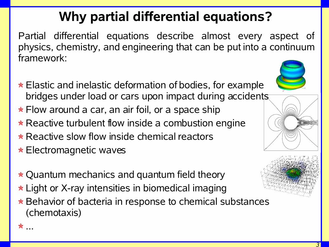
Why partial differential equations?Partial differential equations describe almost every aspect of physics, chemistry, and engineering that can be put into a continuum framework:
Elastic and inelastic deformation of bodies, for example bridges under load or cars upon impact during accidentsFlow around a car, an air foil, or a space shipReactive turbulent flow inside a combustion engineReactive slow flow inside chemical reactorsElectromagnetic waves
Quantum mechanics and quantum field theoryLight or X-ray intensities in biomedical imagingBehavior of bacteria in response to chemical substances (chemotaxis)...
4
Why partial differential equations?PDEs are typically solved by one of the three established methods:
Finite element method (FEM)Finite difference method (FDM)Finite volume method (FVM)
Applying these methods to an equation leads toA large linear or nonlinear system of equations: realistic, three-dimensional problems often have hundreds of thousands or millions of equationsA huge body of work exists on how to solve these resulting systems efficiently (e.g. by iterative linear solvers, multigrid, ...)An equally large body of work exists on the analysis of such methods (e.g. for convergence, stability, ...)A major development of the last 15 years are error estimates
In other words, the numerical solution of PDEs is a mature field.
5
Why optimization?Models (e.g. PDEs) describe how a system behaves if external forcing factors are known and if the characteristics (e.g. material makeup, material properties) are known.
In other words: by solving a known model we can reproduce how a system would react.
On the other hand, this is rarely what we are interested in:
We may wish to optimize certain parameters of a model to obtain a more desirable outcome (e.g. “shape optimization”, “optimal control”, ...)
We may wish to determine unknown parameters in a model by comparing the predicted reaction with actual measurements (“parameter estimation”, “inverse problems”)
6
Why optimization?Optimization also is a mature field:
Many methods are available to deal with the many, often very complicated, aspects of real problems (strong nonlinearities, equality and inequality constraints, ...)
A large body of work exists on the analysis of these methods (convergence, stability)
Many methods are tailored to the efficient solution of problems with many unknowns and many constraints
A huge amount of experience exists on applying these methods to realistic problems in sciences and engineering
7
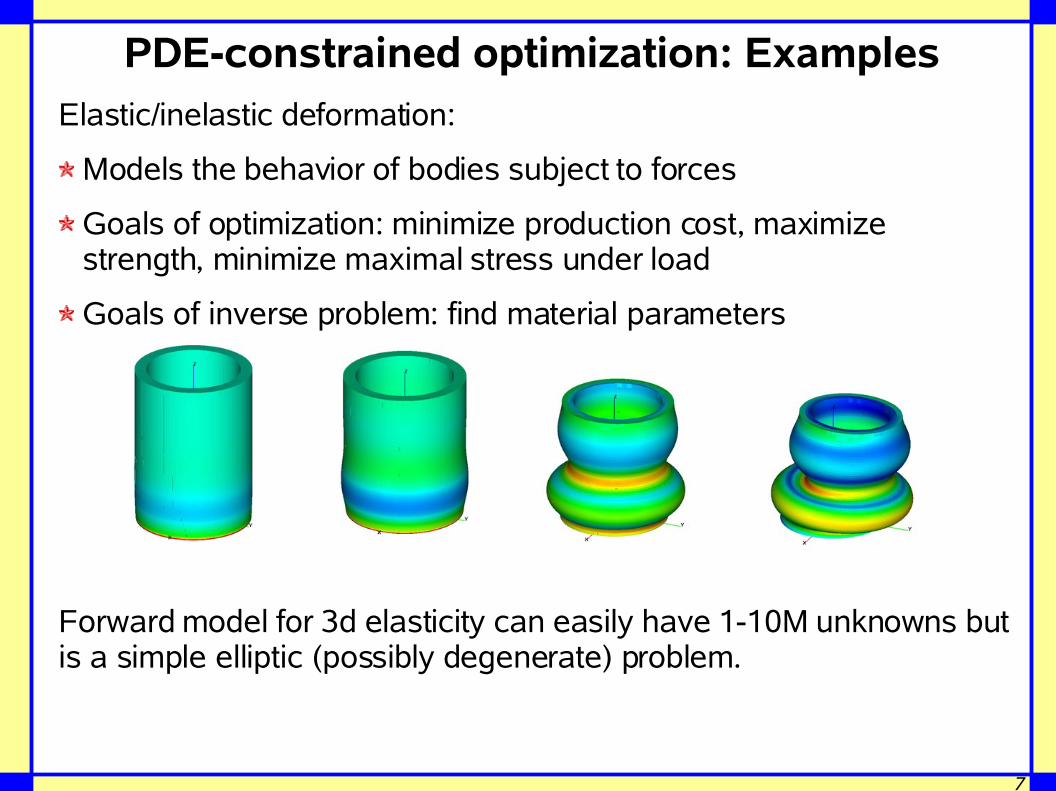
PDE-constrained optimization: ExamplesElastic/inelastic deformation:
Models the behavior of bodies subject to forces
Goals of optimization: minimize production cost, maximize strength, minimize maximal stress under load
Goals of inverse problem: find material parameters
Forward model for 3d elasticity can easily have 1-10M unknowns but is a simple elliptic (possibly degenerate) problem.
8
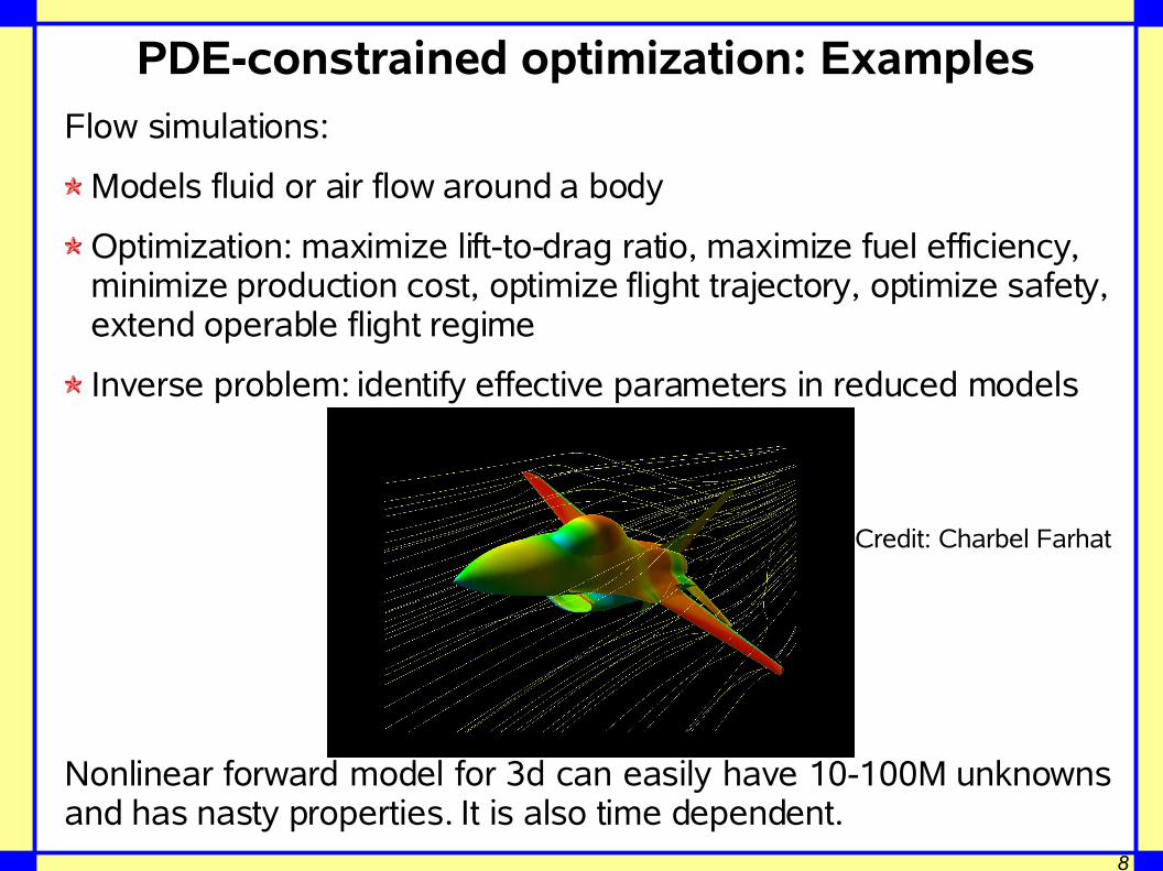
PDE-constrained optimization: ExamplesFlow simulations:
Models fluid or air flow around a body
Optimization: maximize lift-to-drag ratio, maximize fuel efficiency, minimize production cost, optimize flight trajectory, optimize safety, extend operable flight regime
Inverse problem: identify effective parameters in reduced models
Credit: Charbel Farhat
Nonlinear forward model for 3d can easily have 10-100M unknowns and has nasty properties. It is also time dependent.
9
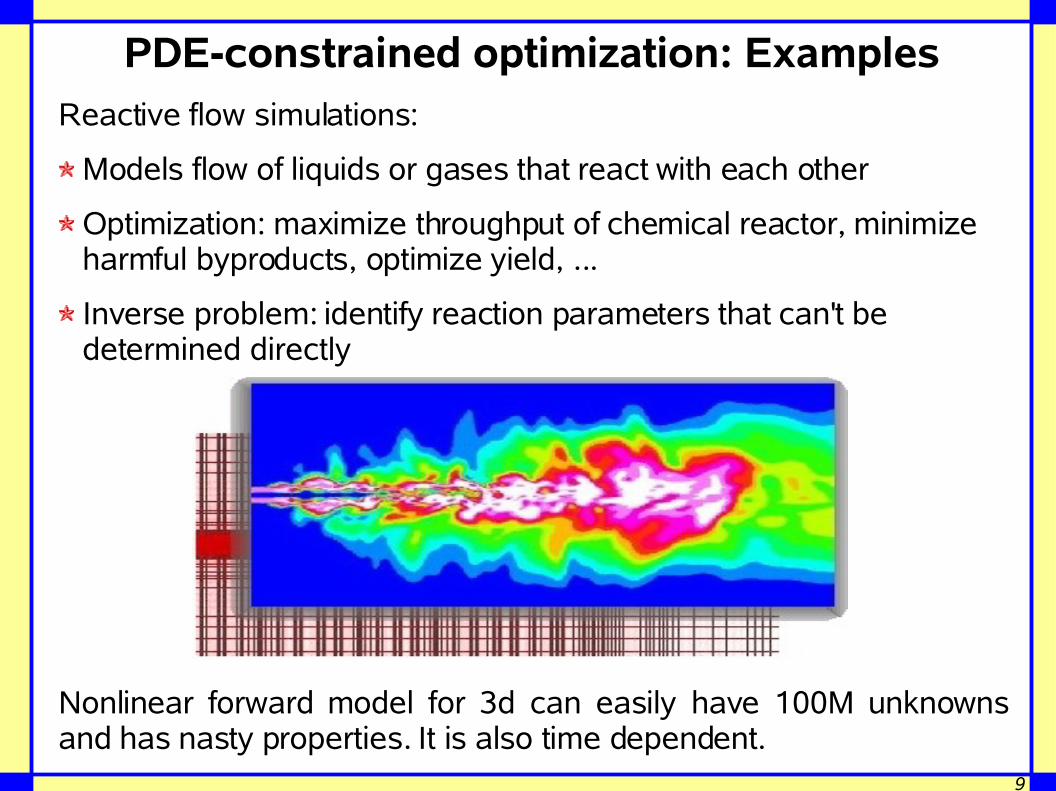
PDE-constrained optimization: ExamplesReactive flow simulations:
Models flow of liquids or gases that react with each other
Optimization: maximize throughput of chemical reactor, minimize harmful byproducts, optimize yield, ...
Inverse problem: identify reaction parameters that can't be determined directly
Nonlinear forward model for 3d can easily have 100M unknowns and has nasty properties. It is also time dependent.
10
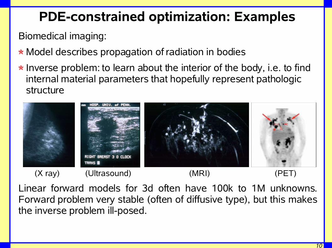
PDE-constrained optimization: ExamplesBiomedical imaging:
Model describes propagation of radiation in bodies
Inverse problem: to learn about the interior of the body, i.e. to find internal material parameters that hopefully represent pathologic structure
(X ray) (Ultrasound) (MRI) (PET)
Linear forward models for 3d often have 100k to 1M unknowns. Forward problem very stable (often of diffusive type), but this makes the inverse problem ill-posed.
`
11
PDE-constrained optimization
So what's the problem – both PDE solution and optimization are mature fields (or so you say)!
From the PDE side:
Many of the PDE solvers use special features of the equations under consideration, but optimization problems don't have them
Optimization problems are almost always indefinite and sometimes ill-conditioned, making the analysis much more complicated
Approaches to error estimation and multigrid are not available for these non-standard problems
There is very little experience (in theory and practice) with inequalities in PDEs
In other words, for PDE guys pretty much everything is new!
12
PDE-constrained optimization
So what's the problem – both PDE solution and optimization are mature fields (or so you say)!
From the optimization side:
Discretized PDEs are huge problems: 100,000s or millions of unknowns
Linear systems are typically very badly conditioned
Model can rarely be solved to high accuracy and doesn't allow for internal differentiation
Maybe most importantly, unknowns are “artificial” since they result from somewhat arbitrary discretization
In other words, for optimization guys pretty much everything is new as well!
13
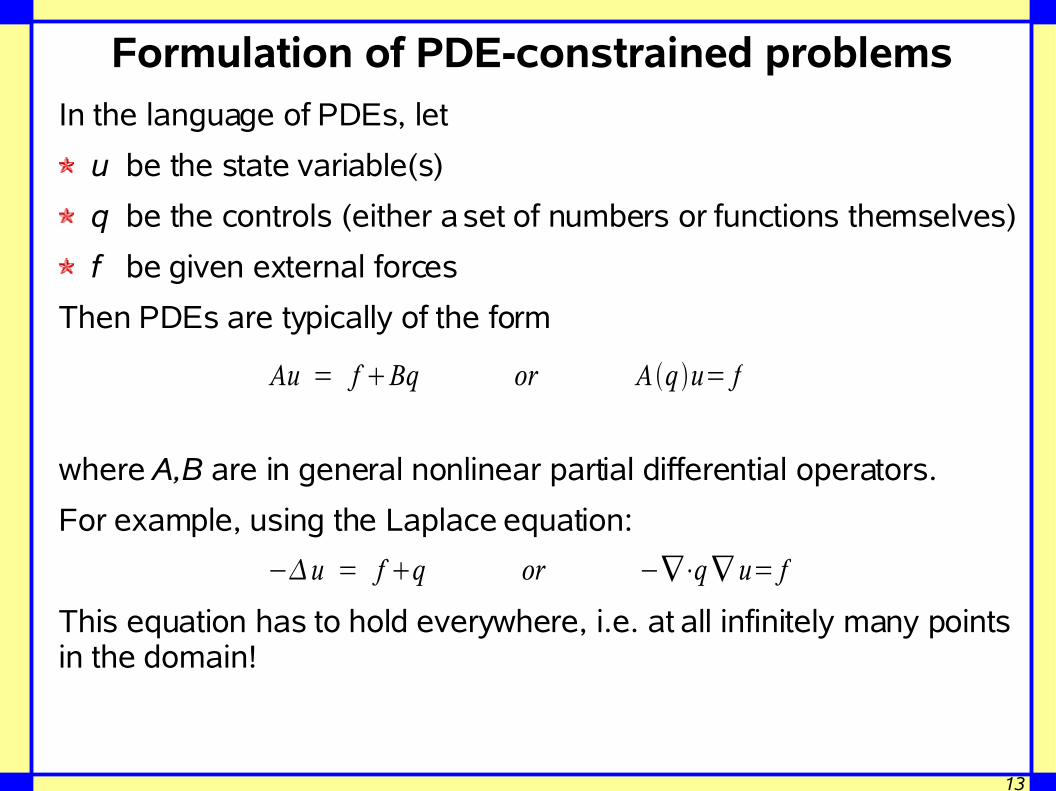
Formulation of PDE-constrained problemsIn the language of PDEs, let
u be the state variable(s)
q be the controls (either a set of numbers or functions themselves)
f be given external forces
Then PDEs are typically of the form
where A,B are in general nonlinear partial differential operators.
For example, using the Laplace equation:
This equation has to hold everywhere, i.e. at all infinitely many points in the domain!
Au = f Bq or A q u= f
−u = f q or −∇⋅q∇ u= f
14
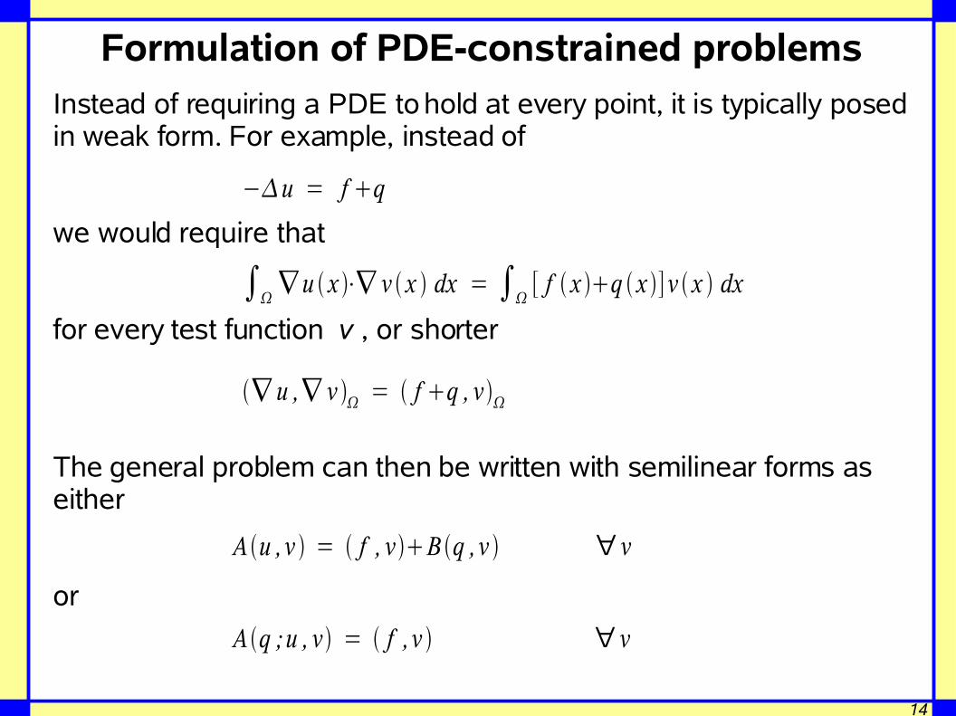
Formulation of PDE-constrained problemsInstead of requiring a PDE to hold at every point, it is typically posed in weak form. For example, instead of
we would require that
for every test function v , or shorter
The general problem can then be written with semilinear forms as either
or
A u , v = f , vB q , v ∀ v
−u = f q
∫∇ u x ⋅∇ v x dx = ∫
[ f x q x ] v x dx
∇ u ,∇ v = f q , v
A q ;u , v = f , v ∀ v
15
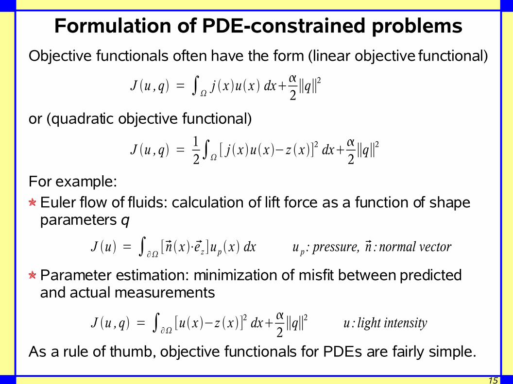
Formulation of PDE-constrained problemsObjective functionals often have the form (linear objective functional)
or (quadratic objective functional)
For example:Euler flow of fluids: calculation of lift force as a function of shape parameters q
Parameter estimation: minimization of misfit between predicted and actual measurements
As a rule of thumb, objective functionals for PDEs are fairly simple.
J u ,q = ∫j x u x dx
2∥q∥2
J u , q = 12∫
[ j x u x −z x ]2 dx2∥q∥2
J u = ∫∂[n x ⋅e z ]u p x dx u p : pressure, n :normal vector
J u , q = ∫∂[u x −z x ]2 dx
2∥q∥2 u : light intensity
16
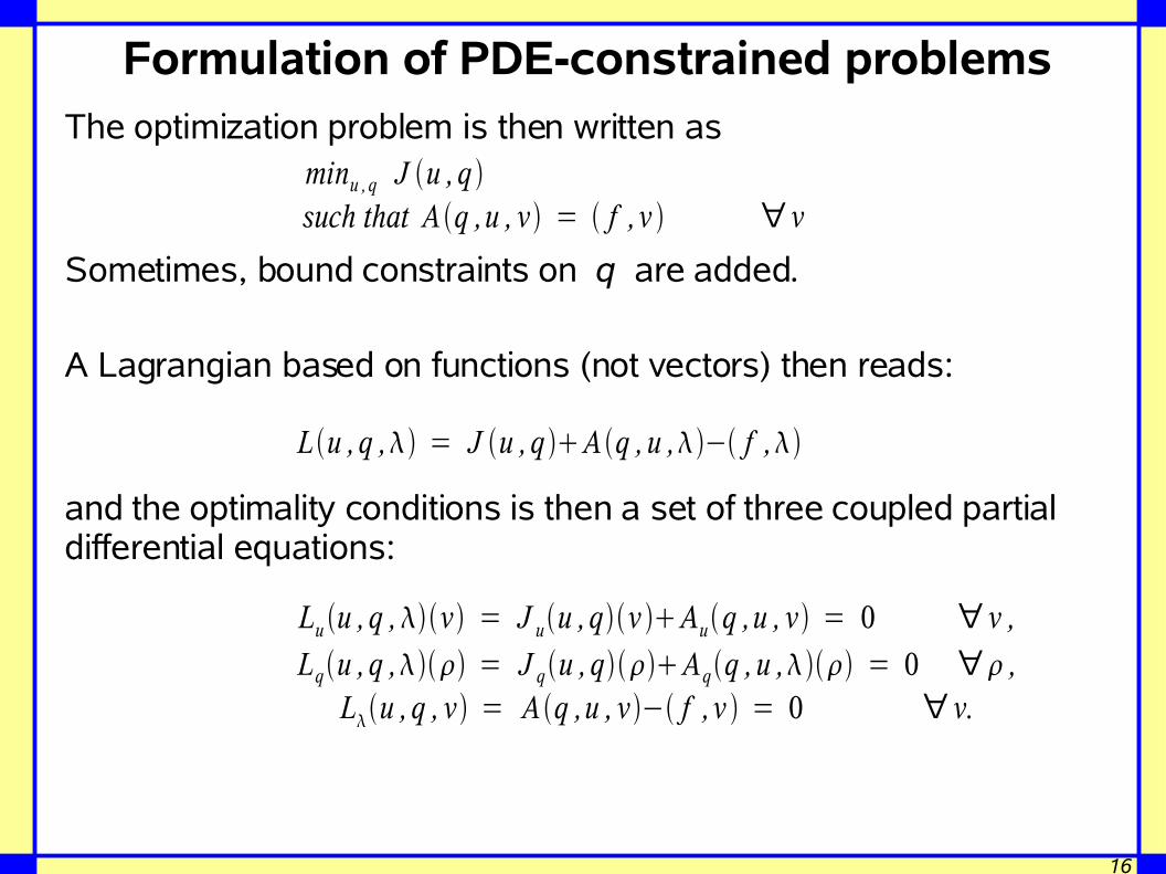
Formulation of PDE-constrained problemsThe optimization problem is then written as
Sometimes, bound constraints on q are added.
A Lagrangian based on functions (not vectors) then reads:
and the optimality conditions is then a set of three coupled partial differential equations:
minu ,q J u ,q such that A q ,u , v = f , v ∀ v
Lu ,q , = J u ,q A q ,u ,− f ,
Lu u , q ,v = J uu ,qv Auq ,u , v = 0 ∀ v ,
Lqu , q , = J qu , qAqq ,u , = 0 ∀ ,Lu , q , v = A q ,u , v− f , v = 0 ∀ v.
17
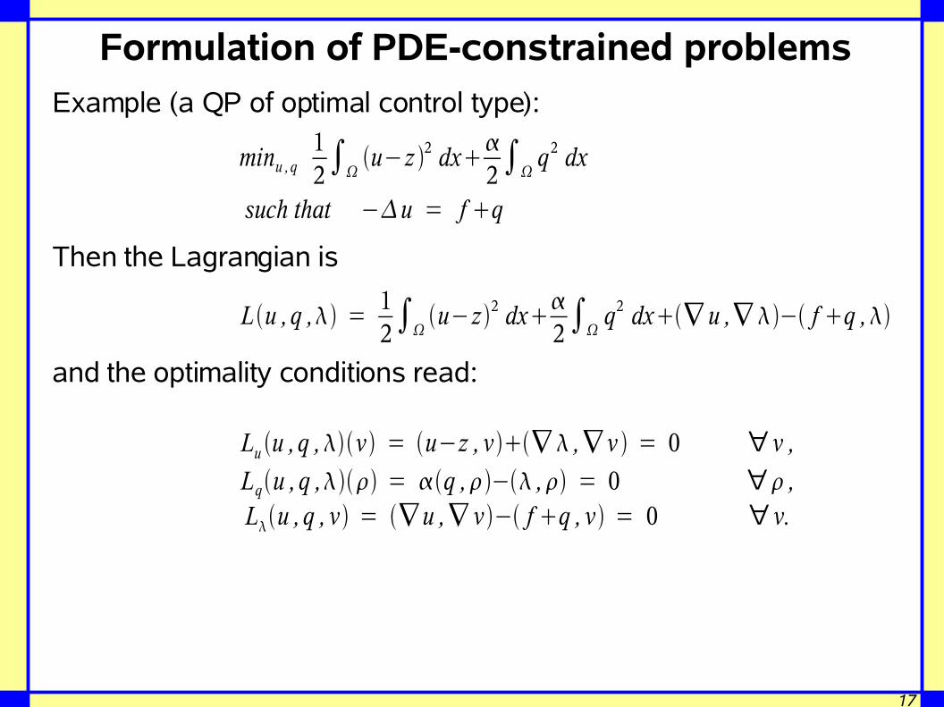
Formulation of PDE-constrained problemsExample (a QP of optimal control type):
Then the Lagrangian is
and the optimality conditions read:
minu ,q 12∫
u−z 2 dx2∫
q2 dx
such that −u = f q
Lu ,q , = 12∫
u−z 2 dx2∫
q2 dx∇ u ,∇− f q ,
Lu u ,q ,v = u−z , v∇ ,∇ v = 0 ∀ v ,
Lqu , q , = q ,− , = 0 ∀ ,Lu , q , v = ∇ u ,∇ v− f q , v = 0 ∀ v.
18
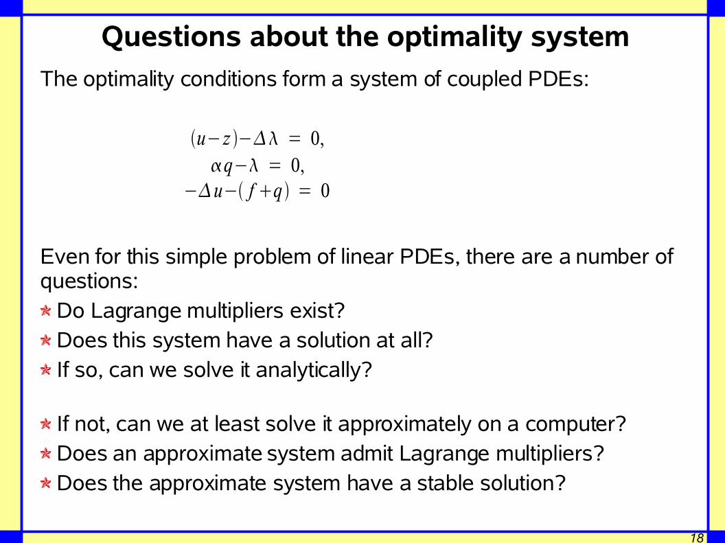
Questions about the optimality systemThe optimality conditions form a system of coupled PDEs:
Even for this simple problem of linear PDEs, there are a number of questions:
Do Lagrange multipliers exist?Does this system have a solution at all?If so, can we solve it analytically?
If not, can we at least solve it approximately on a computer?Does an approximate system admit Lagrange multipliers?Does the approximate system have a stable solution?
u−z − = 0,q− = 0,
−u− f q = 0
19
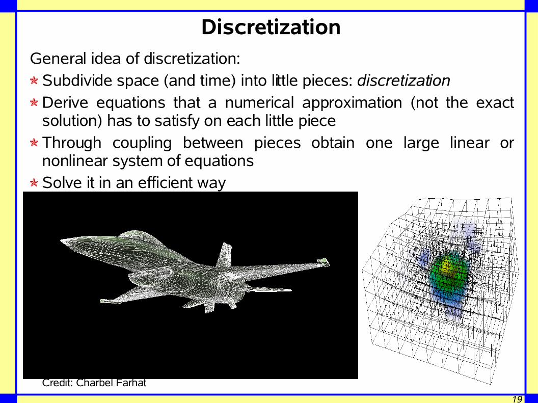
DiscretizationGeneral idea of discretization:
Subdivide space (and time) into little pieces: discretizationDerive equations that a numerical approximation (not the exact solution) has to satisfy on each little pieceThrough coupling between pieces obtain one large linear or nonlinear system of equationsSolve it in an efficient way
Credit: Charbel Farhat

20
DiscretizationIn the finite element method, one replaces the solution u by the ansatz
Clearly, a variational statement like
can then no longer hold since it is unlikely that
However, to determine the N coefficients Ui, we can consider the
following N moments of the equation:
uh x = ∑iU ii x
∇ uh ,∇ v = f , v ∀ v
−uh = f
∇ uh ,∇i = f ,i ∀ i=1...N
21
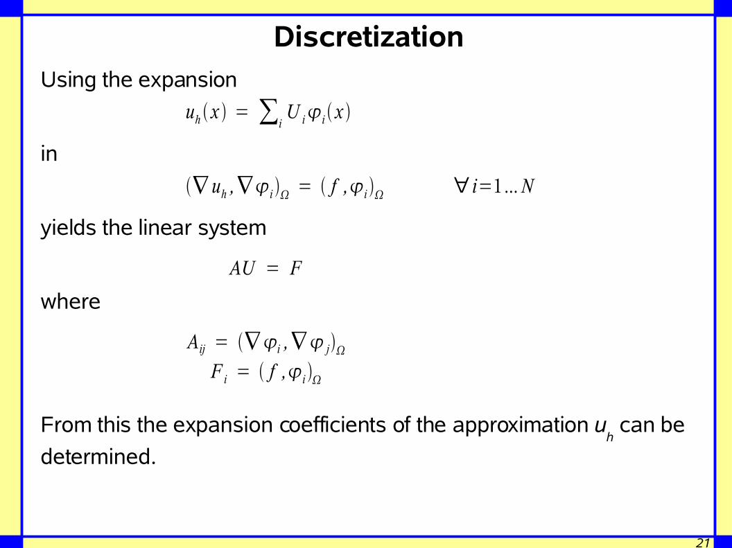
DiscretizationUsing the expansion
in
yields the linear system
where
From this the expansion coefficients of the approximation uh can be
determined.
uh x = ∑iU ii x
AU = F
Aij = ∇i ,∇ jF i = f ,i
∇ uh ,∇i = f ,i ∀ i=1...N
22
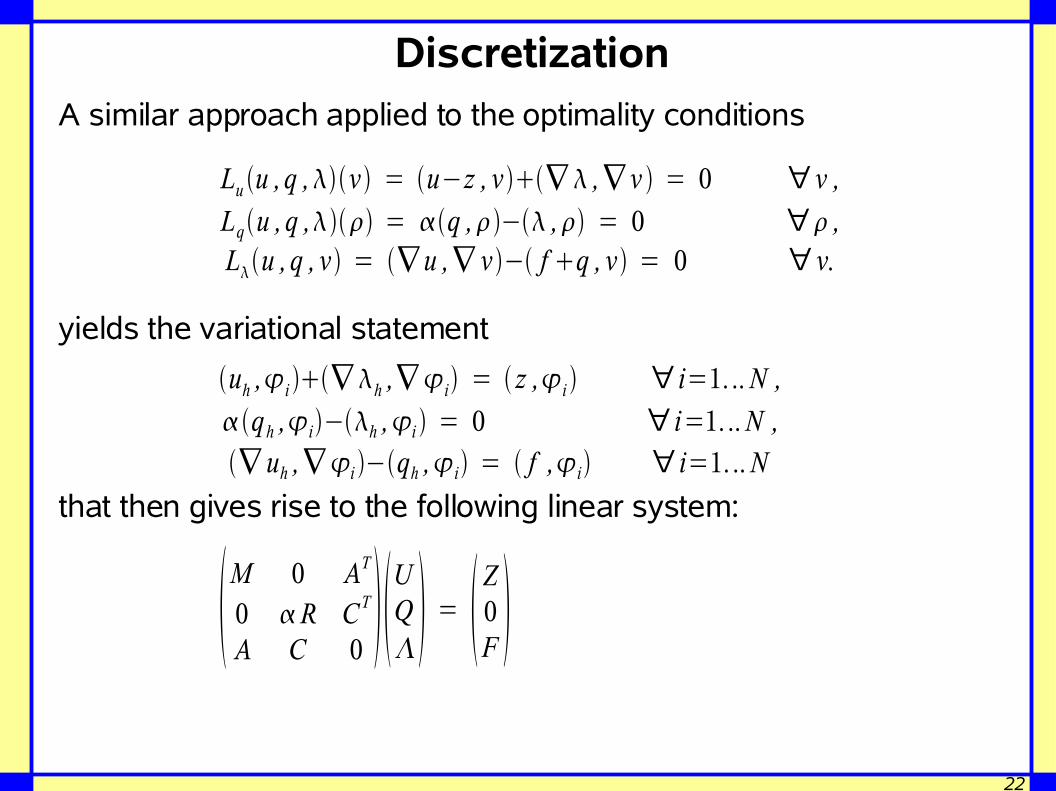
DiscretizationA similar approach applied to the optimality conditions
yields the variational statement
that then gives rise to the following linear system:
Lu u ,q ,v = u−z , v∇ ,∇ v = 0 ∀ v ,
Lqu , q , = q ,− , = 0 ∀ ,Lu , q , v = ∇ u ,∇ v− f q , v = 0 ∀ v.
uh ,i ∇ h ,∇i = z ,i ∀ i=1. ..N ,
qh ,i−h ,i = 0 ∀ i=1. ..N ,
∇ uh ,∇i −qh ,i = f ,i ∀ i=1. ..N
M 0 AT
0 R CT
A C 0 UQ = Z0F
23
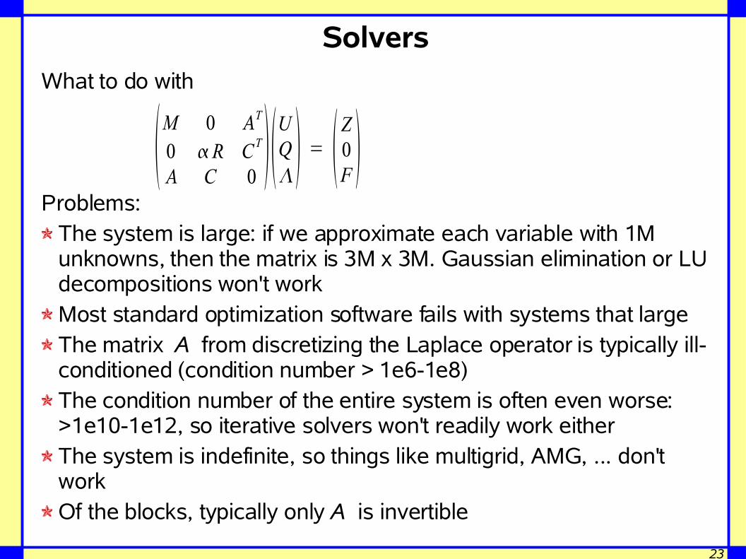
SolversWhat to do with
Problems:The system is large: if we approximate each variable with 1M unknowns, then the matrix is 3M x 3M. Gaussian elimination or LU decompositions won't workMost standard optimization software fails with systems that largeThe matrix A from discretizing the Laplace operator is typically ill-conditioned (condition number > 1e6-1e8)The condition number of the entire system is often even worse: >1e10-1e12, so iterative solvers won't readily work eitherThe system is indefinite, so things like multigrid, AMG, ... don't workOf the blocks, typically only A is invertible
M 0 AT
0 R CT
A C 0 UQ = Z0F
24
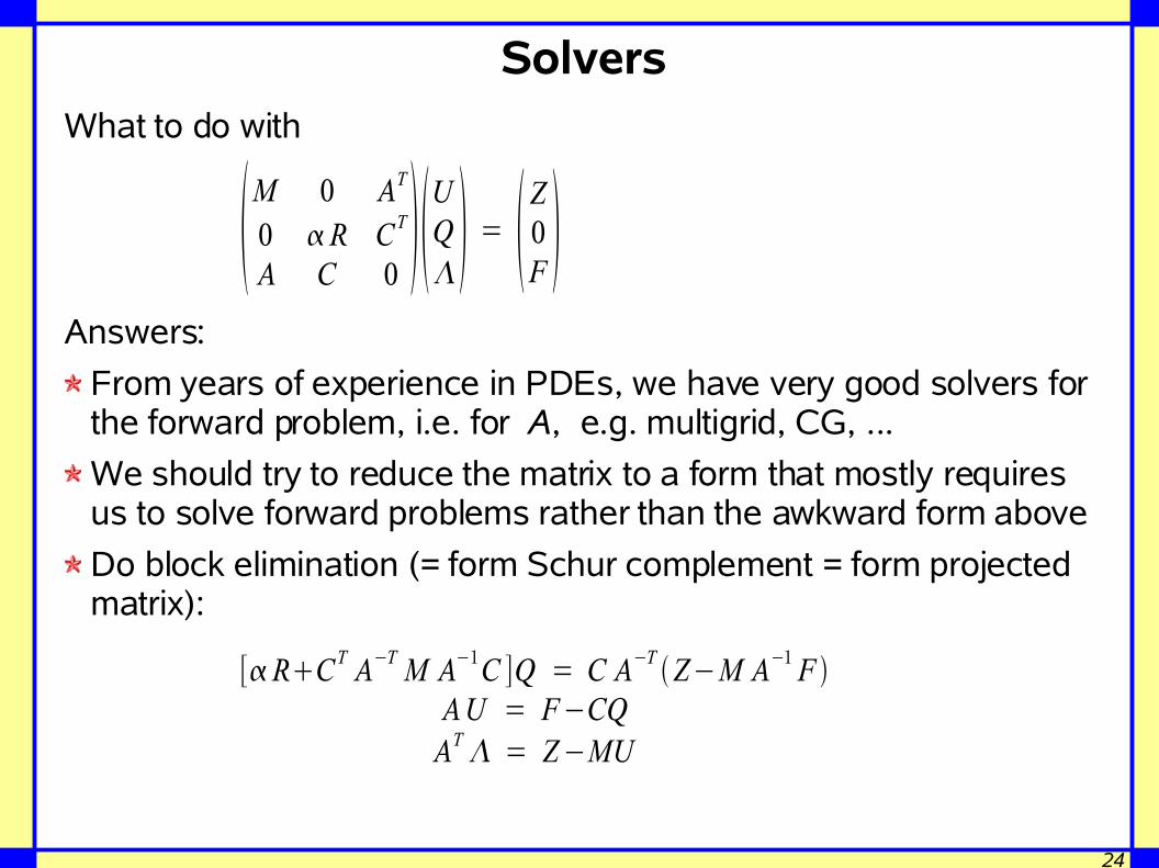
SolversWhat to do with
Answers:
From years of experience in PDEs, we have very good solvers for the forward problem, i.e. for A, e.g. multigrid, CG, ...
We should try to reduce the matrix to a form that mostly requires us to solve forward problems rather than the awkward form above
Do block elimination (= form Schur complement = form projected matrix):
M 0 AT
0 R CT
A C 0 UQ = Z0F
[ RCT A−T M A−1C ]Q = C A−TZ−M A−1 F
A U = F−CQAT = Z−MU
25
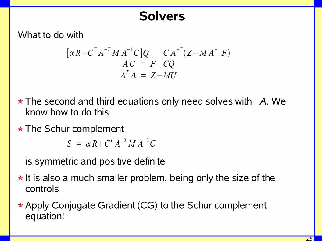
SolversWhat to do with
The second and third equations only need solves with A. We know how to do this
The Schur complement
is symmetric and positive definite
It is also a much smaller problem, being only the size of the controls
Apply Conjugate Gradient (CG) to the Schur complement equation!
[ RCT A−T M A−1C ]Q = C A−TZ−M A−1 F
A U = F−CQAT = Z−MU
S = RCT A−T M A−1C
26
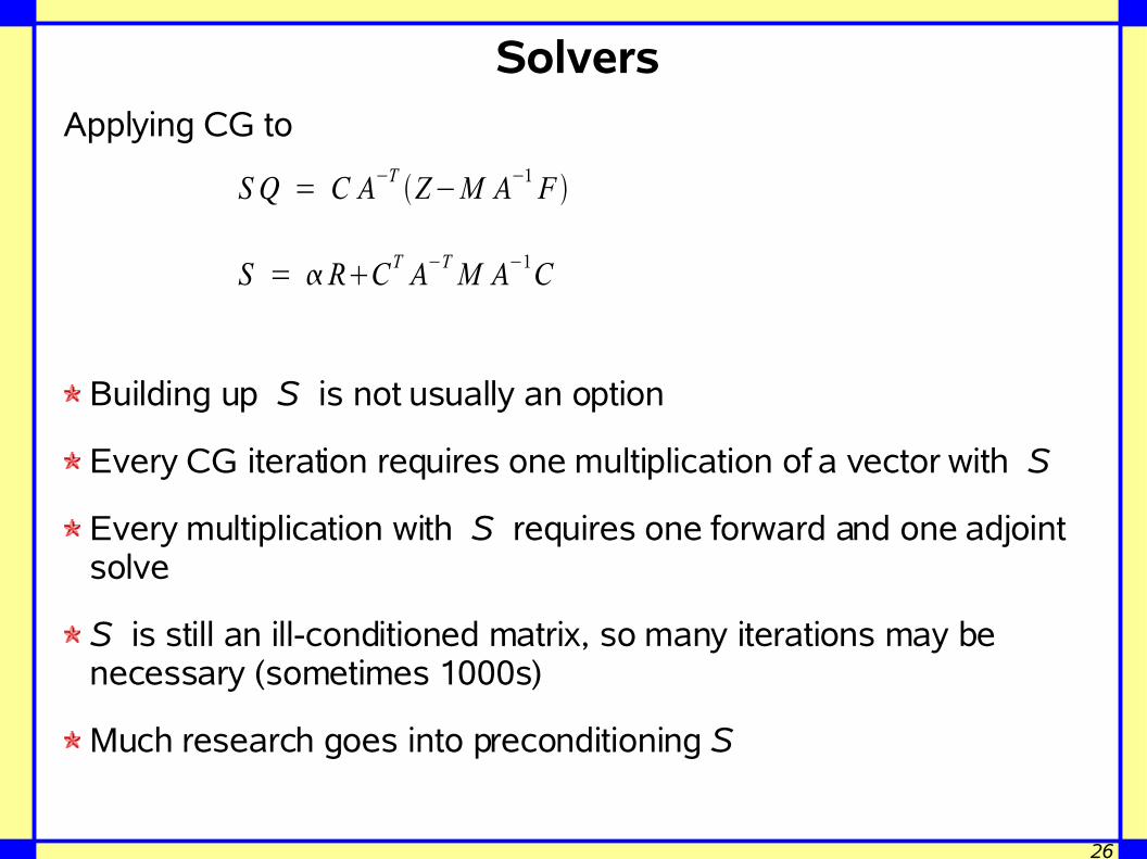
SolversApplying CG to
Building up S is not usually an option
Every CG iteration requires one multiplication of a vector with S
Every multiplication with S requires one forward and one adjoint solve
S is still an ill-conditioned matrix, so many iterations may be necessary (sometimes 1000s)
Much research goes into preconditioning S
S Q = C A−TZ−M A−1 F
S = RCT A−T M A−1C
27
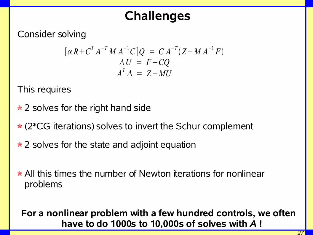
ChallengesConsider solving
This requires
2 solves for the right hand side
(2*CG iterations) solves to invert the Schur complement
2 solves for the state and adjoint equation
All this times the number of Newton iterations for nonlinear problems
For a nonlinear problem with a few hundred controls, we often have to do 1000s to 10,000s of solves with A !
[ RCT A−T M A−1C ]Q = C A−TZ−M A−1 F
A U = F−CQAT = Z−MU
28
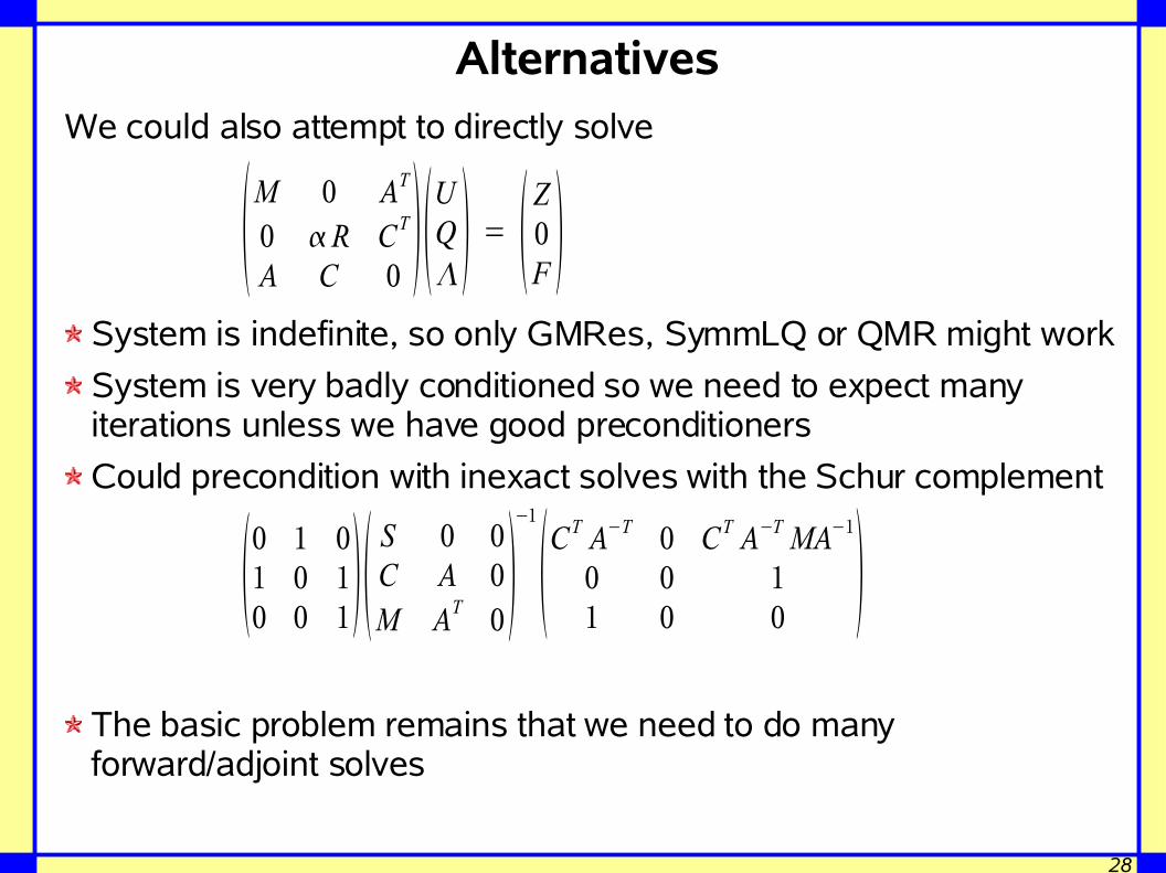
AlternativesWe could also attempt to directly solve
System is indefinite, so only GMRes, SymmLQ or QMR might work
System is very badly conditioned so we need to expect many iterations unless we have good preconditioners
Could precondition with inexact solves with the Schur complement
The basic problem remains that we need to do many forward/adjoint solves
M 0 AT
0 R CT
A C 0 UQ = Z0F
0 1 01 0 10 0 1
S 0 0C A 0M AT 0
−1
CT A−T 0 CT A−T MA−1
0 0 11 0 0
29
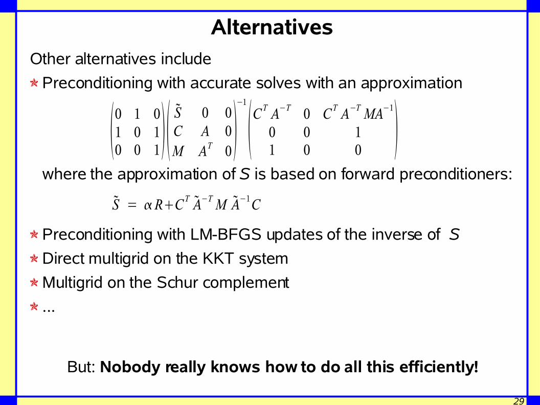
AlternativesOther alternatives include
Preconditioning with accurate solves with an approximation
where the approximation of S is based on forward preconditioners:
Preconditioning with LM-BFGS updates of the inverse of S
Direct multigrid on the KKT system
Multigrid on the Schur complement
...
But: Nobody really knows how to do all this efficiently!
0 1 01 0 10 0 1
S 0 0C A 0M AT 0
−1
CT A−T 0 CT A−T MA−1
0 0 11 0 0
S = RCT A−T M A−1C
30
The basic problem in PDE optimizationFor a nonlinear problem with a few hundred controls, we often
have to do 1000s to 10,000s of solves with A !
For complicated 3d models with a few 100,000 or million unknowns, every forward solve can easily cost minutes, bringing the total compute time into hours/days/weeks.
This gets even worse if we have time-dependent problems.
And all this even though we have a fairly trivial optimization problem:
Convex objective function (but possibly nonlinear constraints)
No state constraints (though possibly control constraints of bounds type)
No complicated other constraints.
31
Summary and outlookTo date, PDE-constrained optimization problems are fairly trivial but huge from an optimization perspective, but moderately large and very complex from a PDE perspective
Even solving the most simple problems is considered frontier research
Because efficient linear solvers for the saddle point problems like the ones originating from optimization are virtually unknown, one tries to go back to forward solvers through the Schur complement
Inclusion of bounds on controls allows to keep this structure
Inclusion of state constraints would yield a variational inequality that requires different techniques and for which we don't have solvers yet
Multiple experiment parameter estimation problems can also make the computational complexity very large
32
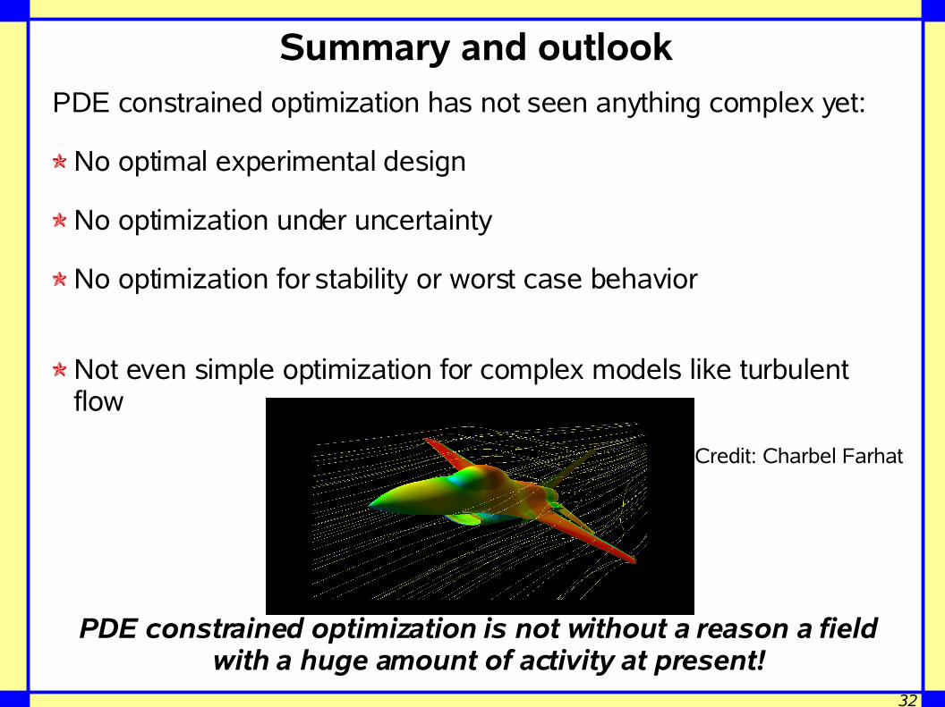
Summary and outlookPDE constrained optimization has not seen anything complex yet:
No optimal experimental design
No optimization under uncertainty
No optimization for stability or worst case behavior
Not even simple optimization for complex models like turbulent flow
Credit: Charbel Farhat
PDE constrained optimization is not without a reason a field with a huge amount of activity at present!


