An introduction to R William Revelle Swift 315 email: [email protected]March 29, 2009 Contents 1 Objectives 1 2 Requirements and readings 2 3 Day 1: What is R? An introduction 2 3.1 What is it? .................................... 2 3.2 How to get it: CRAN (Comprehensive R Archive Network) ......... 3 3.3 Packages and Task Views ............................ 4 3.4 Help and Guidance ................................ 4 3.5 Package vignettes ................................. 5 3.6 Basic R commands and syntax ......................... 5 3.6.1 R is just a fancy calculator ....................... 5 3.6.2 R as a graphing calculator ........................ 7 3.6.3 R is also a statistics table ........................ 10 3.6.4 R will make up data ........................... 12 4 Entering or getting the data 12 4.1 Getting data from a remote file server ..................... 12 4.2 Getting data from a local file .......................... 15 4.3 Copying the data from the clipboard ...................... 15 4.4 Reading from an SPSS file ............................ 15 4.5 Getting the data from a built in data set .................... 16 4.6 Entering data manually–understanding data structures ............ 16 4.6.1 Data structures .............................. 16 4.6.2 Entering data into a data.frame ..................... 19 4.7 Basic data manipulation ............................. 20 1
10 Day 5: R as a programming language 3810.1 R in the lab . . . . . . . . . . . . . . . . . . . . . . . . . . . . . . . . . . . . 3810.2 R in the classroom . . . . . . . . . . . . . . . . . . . . . . . . . . . . . . . . 3810.3 Using R and Latex or OpenOffice to prepare documents . . . . . . . . . . . 38
11 Various web resources 38
This short course will meet in Swift Hall 107 from 5-7 on Monday, Tuesday, Wednesday(March 30-April 1) and Monday, Tuesday (April 6-7).
2
1 Objectives
There are many possible statistical programs that can be used in psychological research.They differ in multiple ways, at least some of which are ease of use, generality, and cost.Some of the more common programs used are SAS, SPSS, and Systat. These programshave GUIs (Graphical User Interfaces) that are relatively easy to use but that are uniqueto each package. These programs are also very expensive and limited in what they can do.Although convenient to use, GUI based operations are difficult to discuss in written form.When teaching statistics or communicating results, it is helpful to use examples that othersmay use, perhaps in other computing environments. This course describes an alternativeapproach that is widely used by practicing statisticians, the statistical environment R.
R is used in various courses here at NU and has been adopted as the primary stats programfor teaching at the University of Virginia and the University of Colorado (among others).I use it in teaching Psych 205, 371, 405, and 454.
The objective of this short course is very simple: to have you learn enough about R to startusing it to facilitate your teaching and research. You will not, however be fluent in R. But,by the end of the course you should be wondering why you ever used SPSS or SAS. For“this is R. There is no if. Only how.” (R fortune).
2 Requirements and readings
A willingness to learn and to ask questions. Bringing a personal computer to class wouldnot be a bad idea.
Handouts of the lecture notes will be linked from this outline. Most of the handouts willbe either pdfs of slides or pdfs of example code.
There are a number of tutorials on learning R, ranging from the short to the extensive. Thedefinitive short text is An Introduction to R by Venables et al. (2008). This may either bepurchased (proceeds go to the R Foundation) or downloaded. For those who are familiarwith SPSS or SAS, the book, R for SAS and SPSS Users by Muenchen (2009), is a goodintroduction. (See his webpage at http://rforsasandspssusers.com/). For psychologists, mytutorial Using R for psychological research:A simple guide to an elegant package is not abad beginning. See also the short and very short versions of that for undergraduates. Asan example of what a bright undergraduate can do to help other undergraduates use R,see K. Funkhouser’s Using R to analyze a simple data set.
There are a number of other very good tutorials on the web. An essential aid is the Rreference card and the search engines R seek: a search engine for R and Jonathan Baron’ssearch engine of the R help archives.
The R Development Core Team (2008) has developed an extremely powerful “languageand environment for statistical computing and graphics” and a set of packages that operatewithin this programming environment (R). The R program is an open source version of thestatistical program S and is very similar to the statistical program based upon S, S-PLUS(also known as S+). Although described as merely “an effective data handling and storagefacility [with] a suite of operators for calculations on arrays, in particular, matrices” Ris, in fact, a very useful interactive package for data analysis. When compared to mostother stats packages used by psychologists, R has at least three compelling advantages:it is free, it runs on multiple platforms (e.g., Windows, Unix, Linux, and Mac OS Xand Classic), and combines many of the most useful statistical programs into one quasiintegrated environment. R is free1, open source software as part of the GNU2 Project. Thatis, users are free to use, modify, and distribute the program, within the limits of the GNUnon-license). The program itself and detailed installation instructions for Linux, Unix,Windows, and Macs are available through CRAN (Comprehensive R Archive Network) athttp://www.r-project.org
The R Development Core Team (2008) releases an updated version of R about every sixmonths. That is, as of March, 2009, the current version of 2.8.1 will be replaced with 2.9.0sometime in April. Bug fixes are then added with a sub version number (e.g. 2.8.1 fixedminor problems with 2.8.0). It is recommended to use the most up to date version, as itwill incorporate various improvements and operating efficiencies. Although many run R asa language and text oriented programming environment, there are GUIs available for PCs,Linux and Macs. See for example, R Commander by John Fox or R-app for the Macintoshdeveloped by Stefano Iacus and Simon Urbanek. Compared to the basic PC environment,the Mac GUI is to be preferred.
R is an integrated, interactive environment for data manipulation and analysis that includesfunctions for standard descriptive statistics (means, variances, ranges) and also includesuseful graphical tools for Exploratory Data Analysis. In terms of inferential statistics Rhas many varieties of the General Linear Model including the conventional special casesof Analysis of Variance, MANOVA, and linear regression. Statisticians and statisticallyminded people around the world have contributed packages to the R Group and maintaina very active news group offering suggestions and help. The growing collection of pack-ages and the ease with which they interact with each other and the core R is perhaps thegreatest advantage of R. Advanced features include correlational packages for multivariate
1Free as in speech rather than as in beer. See http://www.gnu.org2GNU’s Not Unix
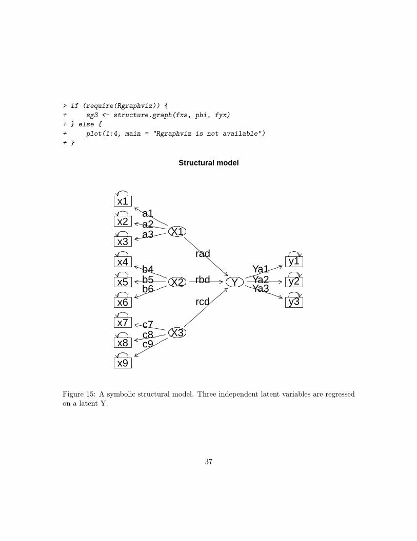
analyses including Factor and Principal Components Analysis, and cluster analysis. Ad-vanced multivariate analyses packages that have been contributed to the R-project includeone for Structural Equation Modeling (sem, Hierarchical Linear Modeling (referred to asnon linear mixed effects in the nlme4 package) and taxometric analysis. All of these areavailable in the (>1400) free packages distributed by the R group at CRAN. Many of thefunctions described in this book are incorporated into the psych package. Other packagesuseful for psychometrics are described in a task-view at CRAN. In addition to being aenvironment of prepackaged routines, R is a interpreted programming language that allowsone to create specific functions when needed.
R is also an amazing program for producing statistical graphics. A collection of some of thebest graphics is available at the webpage addictedtoR with a complete gallery of thumbnailof figures.
3.2 How to get it: CRAN (Comprehensive R Archive Network)
Although it is possible that your local computer lab already has R, it is most useful to doanalyses on your own machine. In this case you will need to download the R program fromthe R project and install it yourself. Go to the R home page at http://www.r-project.organd then choose the Download from CRAN (Comprehensive R Archive Network) option.This will take you to list of mirror sites around the world. You may download the Windows,Linux, or Mac versions at this site. For most users, downloading the binary image is easiestand does not require compiling the program.
3.3 Packages and Task Views
One of the advantages of R is that it can be supplemented with additional programs thatare included as packages using the package manager. (e.g., sem does structural equa-tion modeling) or that can be added using the source command. Most packages aredirectly available through the CRAN repository. Others are available at the BioConductorhttp://www.bioconductor.org repository. Yet others are available at “other” reposito-ries. The psych package Revelle (2009) may be downloaded from CRAN or from the http://personality-project.org/r repository. The concept of a “task view” has made down-loading relevant packages very easy. For instance, the install.views("psychometrics")command will download over 20 packages that do various types of psychometrics.
For any other than the default packages to work, you must activate it by either using thePackage Manager or the library command:
• entering ?psych will give a list of the functions available in the psych package as wellas an overview of their funtionality.
• objects(package:psych) will list the functions available in a package (in this case,psych).
3.4 Help and Guidance
R is case sensitive and does not give overly useful diagnostic messages. If you get an errormessage, don’t be flustered but rather be patient and try the command again using thecorrect spelling for the command.
When in doubt, use the help(somefunction) function. This is identical to ? somefunctionwhere some function is what you want to know about. e.g.,?read.table #ask for help in using the read.table function – see the answer in the helpwindow, orhelp(read.table) #another way of asking for help. - see the help window
RSiteSearch(“keyword”) will open a browser window and return a search for “keyword” inall functions available in Rand the associated packages as well (if desired) the R-Help Newsgroups.
3.5 Package vignettes
All packages have help pages for each function in the package. These are meant to help youuse a function that you already know about, but not to introduce you to new functions. Anincreasing number of packages have a package “vignettes” that give more of an overview ofthe program than a detailed description of any one function. These vignettes are accessiblefrom the help window and sometimes as part of the help index for the program. The twovignettes for the psych package are also available from the personality project web page.(An overview of the psych package and Using the psych package as a front end to the sempackage).
3.6 Basic R commands and syntax
There are more than 10,000 possible one line commands that one can enter when usingR 3 and no one can be expected to know them all. Even those of us who write packagesneed help remembering the possible commands and syntax of our own packages. In fact,
3This is based on the observation that there are > 1500 packages and that each package probably hasat least 6 functions.
the Rpad handout is just one of many ways of remembering the appropriate command forcore R. Even so, the basic concept of all commands is fairly easy to grasp in terms of thefollowing simple analogy: R is just a fancy calculator that draws graphics and has built instatistic tables.
3.6.1 R is just a fancy calculator
One can think of R as a fancy graphics calculator. Enter a command and look at theoutput. Thus,
> 2 + 2
[1] 4
> 3^4
[1] 81
> pi
[1] 3.141593
In the above example, the > symbol is the R prompt and the next line [1] is the answer.When copying a line like this, do not include the > symbol. The # symbol is used to addcomments to lines (and will not show when running R to prepare documents!). It is helpfulto use a text editor (perhaps the one available in R, perhaps another one) to write thecommands out before copying them into R. The up arrow command will echo the previouscommand on the terminal and allow for editing.
At the abstract level, almost all operations in R consists of executing a function on anobject. The result is a new object. This very simple idea allows the output of any operationto be operated on by another function.
Command syntax tends to be of the form:variable = function (parameters) orvariable <- function (parameters)The = and the <- symbol imply replacement, not equality. The preferred style is to usethe <- symbol to avoid confusion with the test for equality (==).
The result of an operation will not necessarily appear unless you ask for it. The commandx <- c(1, 3, 5, 7)m <- mean(x)will create the vector x made up of the numbers 1, 3, 5, 7, and set m equal to the mean ofx but will not print anything on the console without the additional requestm.
however, just asking mean(x)will find the mean and print it.
> x <- c(1, 3, 5, 7)
> m <- mean(x)
> m
[1] 4
> mean(x)
[1] 4
> sd(x)
[1] 2.581989
In addition to simple arithmetic, R allows you to create vectors or matrices and do oper-ations on these matrices. The first example forms the vector V made up of the numbersfrom 1 to 10. The second finds the 3 x 5 matrix, m, made up of randomly chosen numberssampled (with replacement) from the numbers 0-9. In this later example, to make theexample replicable for the reader, the random number seed is set to a well known but arbi-trary value (Adams, 1980). Using the fancy desk calculator ability of R, the last operationis a matrix operation that finds the sum of the cross products of M. That is, the sum of thesquares of the columns of M (the diagonals) and the sum of the products of each columnwith each other column.
Suppose we want to present a graph comparing two normal distributions with differentmeans and sigmas:
3.6.3 R is also a statistics table
It has been suggested by some that you should never buy a statistics book that has proba-bility tables in it, because that means that the author did not know about modern statisticsand the various distributions in R. Many statistics books include tables of the t or F orχ2 distribution. By using R this is unnecessary since these and many more distributionscan be obtained directly. Consider the normal distribution as an example. dnorm(x,mean=mu, sd=sigma) will give the probability density of observing that x in a distribu-tion with mean=mu and standard deviation= sigma. pnorm(q,mean=0,sd=1) will givethe probability of observing the value q or less. qnorm(p, mean=0, sd=1) will give thequantile value of a value with probability p. rnorm(n,mean,sd) will generate n randomobservations sampled from the normal distribution with specified mean and standard de-viation. Thus, to find out what z value has a .05 probability we ask for qnorm(.05). Or,to evaluate the probability of observing a z value of 2.5, specify pnorm(2.5). (These lasttwo examples are one side p values).
Applying these prefixes (d,p,q, r) to the various distributions available in R allows us toevaluate or simulate many different distributions (Table 1).
Consider the following examples.
> pt(2, 6)
9
> curve(dnorm(x, 1, 0.5), -3, 3, ylab = "Probability of x", main = "Comparing two distributions")
> curve(dnorm(x, 0, 1), add = TRUE)
−3 −2 −1 0 1 2 3
0.0
0.2
0.4
0.6
0.8
Comparing two distributions
x
Pro
babi
lity
of x
Figure 1: Two normal distributions drawn using the curve function.
10
−3 −2 −1 0 1 2 3
0.0
0.1
0.2
0.3
0.4
The normal curve
Pro
babi
lity
of z
Figure 2: The normal curve with various colorings is a nice example of a simple but usefulgraphic.
11
[1] 0.9537868
> pnorm(2)
[1] 0.9772499
> dnorm(-1)
[1] 0.2419707
> pf(3.5, 1, 20)
[1] 0.923926
> qf(0.95, 1, 60)
[1] 4.001191
> qchisq(0.95, 1)
[1] 3.841459
3.6.4 R will make up data
Although making up data is normally considered a bad thing for a researcher to do, whenwe call it“simulation” it is considered scientific. All of the distributions listed in Table 1 canbe prefaced with “r” to create (pseudo) random data with that particular shape. Considerthe following example where the data are generated and then their histogram is drawn(Figure 3).
This ability to simulate data is particularly useful when teaching statistics, or when tryingout a new method. For if you know what the underlying model is, it is easier to understandwhat how well the method works. When teaching about distributions, it is useful to showwhat happens if we take progressively larger samples of the data. This is shown in Figure 4where we plot the means of samples of size 1, 2, 4, and 8. This uses the replicate androwMeans functions. The last two panels show how to combine multiple commands intoone line.
4 Entering or getting the data
For most data analysis, rather than manually enter the data into R, it is probably moreconvenient to use a spreadsheet (e.g., Excel or OpenOffice) as a data editor, save as a tabor comma delimited file, and then read the data from the file. Many of the examples inthis tutorial assume that the data have been entered this way. Many of the examples in
12
Table 1: Some of the most useful distributions for psychometrics that are available asfunctions. To obtain the density, prefix with d, probability with p, quantiles with q andto generate random values with r. (e.g., the normal distribution may be chosen by usingdnorm, pnorm, qnorm, or rnorm.) Each function has specific parameters, some of whichtake default values, some of which require being specified. Use help for each function fordetails.
Distribution base name P 1 P 2 P 3 example applicationNormal norm mean sigma Most data
Multivariate normal mvnorm mean r sigma Most dataLog Normal lnorm log mean log sigma income or reaction time
Uniform unif min max rectangular distributionsBinomial binom size prob Bernuilli trials (e.g. coin flips)
Student’s t t df nc Finding significance of a t-testMultivariate t mvt df corr nc Multivariate applications
Fisher’s F f df1 df2 nc Testing for significance of F testχ2 chisq df nc Testing for significance of χ2
Beta beta shape1 shape2 nc distribution theoryCauchy cauchy location scale Infinite variance distribution
Hypergeometric hyper m n kLogistic logis location scale Item Response TheoryPoisson pois lambda Count dataWeibull weibull shape scale Reaction time distributions
13
> op <- par(mfrow = c(2, 2))
> n <- 1000
> x <- rnorm(n)
> hist(x, main = "Normal")
> x <- runif(n)
> hist(x, main = "Rectangular")
> x <- rpois(n, 3)
> hist(x, main = "Poisson")
> x <- rlnorm(n)
> hist(x, main = "Log Normal")
> op <- par(mfrow = c(1, 1))
Normal
x
Fre
quen
cy
−3 −1 0 1 2 3
050
100
200
Rectangular
x
Fre
quen
cy
0.0 0.2 0.4 0.6 0.8 1.0
040
8012
0
Poisson
x
Fre
quen
cy
0 2 4 6 8 10
050
100
200
Log Normal
x
Fre
quen
cy
0 10 20 30 40
020
060
0
Figure 3: Histograms of four different random distributions, the normal (rnorm), the rect-angular or uniform (runif), the Poisson (rpois), and the lognormal (rlnorm). The first opcommand specifies that we want a 2 x 2 plot, the second one returns us to the normal 1 x1 plot.
> hist(rowMeans(replicate(8, runif(n))), main = "8 cases", xlim = c(0, 1), xlab = "Mean of x")
> op <- par(mfrow = c(1, 1))
1 case
x
Fre
quen
cy
0.0 0.2 0.4 0.6 0.8 1.0
020
6010
0
2 cases
x
Fre
quen
cy
0.0 0.2 0.4 0.6 0.8 1.0
050
100
150
200
4 cases
rowMeans(replicate(4, runif(n)))
Fre
quen
cy
0.0 0.2 0.4 0.6 0.8 1.0
050
150
250
8 cases
Mean of x
Fre
quen
cy
0.0 0.2 0.4 0.6 0.8 1.0
050
100
200
Figure 4: Histograms of the means of four different sample sizes where the samples aretaken from a uniform distribution. This makes use of the replicate and rowSums functions,as well as the runif and hist functions.
15
the help menus have small data sets entered using the c() command or created on the fly.It is also possible to read data in from a remote file server. Alternatively, if you have datain a SAS or SPSS file, there are functions in the foreign package to import them.
Using the copy.clipboard() function from the psych package, it is also possible to havea data file open in a text editor or spreadsheet program, copy the relevant lines to theclipboard, and then read the clipboard directly into R.
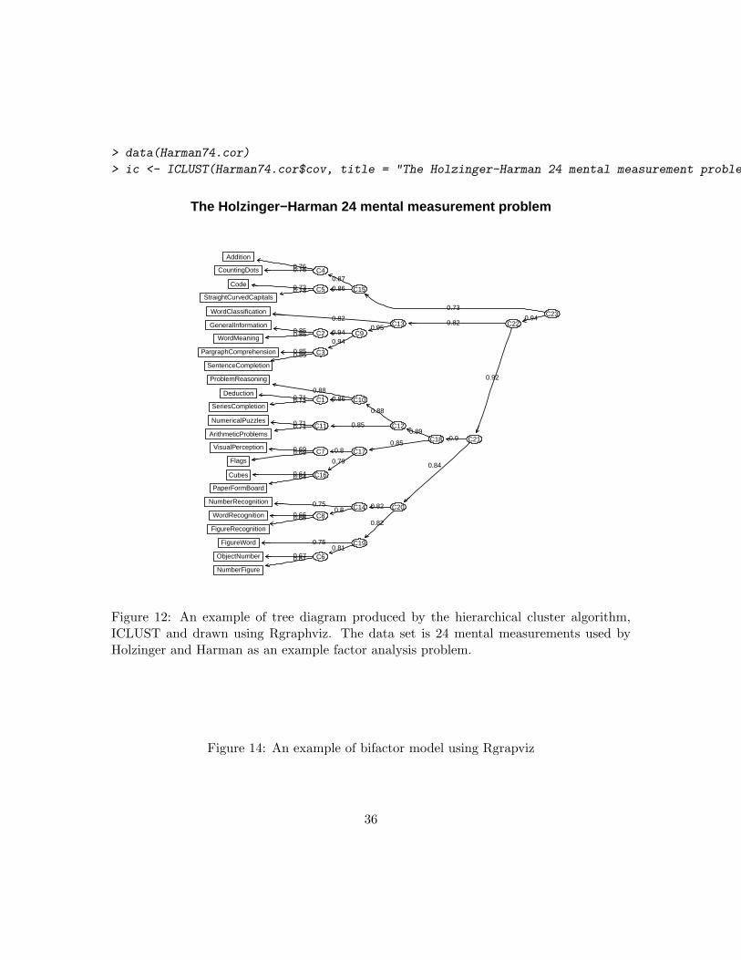
Finally, many packages include example data sets that can be accessed directly using thedata command. Thus, to get a number of factor analysis examples with a bifactor structure,the bifactor data set is called to make the seven data sets within it available.
4.1 Getting data from a remote file server
For the first example, we read data from a file server in the Personality-Motivation-Cognition lab at Northwestern University that contains the responses for several hundredsubjects on 13 personality scales (5 from the Eysenck Personality Inventory (EPI), 5 froma Big Five Inventory (BFI) , one Beck Depression, and two anxiety scales). The data aretaken from a study in the Personality, Motivation, and Cognition Laboratory. The file isstructured normally, i.e. rows represent different subjects, columns different variables, andthe first row gives subject labels. Had we saved this file as comma delimited, we wouldadd the separation (sep=”,”) parameter.
> my.data <- read.table(datafilename,header=TRUE) #read the data file
4.2 Getting data from a local file
More typically, the data are stored somewhere on your computer in a tab delimited orcomma delimited file. The process is equally easy, in that you first locate the file and thenread it.
> datafilename <- file.choose() #where you dynamically can go to find the file
> my.data <- read.table(datafilename,header=TRUE) #read the data file
4.3 Copying the data from the clipboard
Yet another alternative is to directly access the data file outside of R, copy the data to theclipboard, and then read the clipboard using the read.clipboard function.
16
> my.data <- read.clipboard() # if there are complete cases and each column has an identifier
> my.data <- read.clipboard(header=FALSE) # if there are complete cases and columns do not have identifiers
> my.data <- read.clipboard(sep="t") #if the data come from a spreadsheet with blank cells to represent missing data
> my.data <- read.clipboard.csv() #if the data were copied from a comma delimited file
4.4 Reading from an SPSS file
To read from an SPSS or SAS data file, it is necessary to first load the foreign.
> library(foreign)
> my.spss.file.name <- file.choose() #where you dynamically can go to find the file
Because we want to demonstrate the same data set many times and the user is not nec-essarily connected to the internet, many packages have built in data sets. A list of allavailable sets can be found by the data() command. The data sets within a package arefound by specifying the package. For the next examples, we use the epi.bfi data set.
> data(package = "psych")
> data(epi.bfi)
> my.data <- epi.bfi
The data are now in the data.frame “my.data”. Data.frames allow one to have columnsthat are either numeric or alphanumeric. They are conceptually a generalization of a matrixin that they have rows and columns, but unlike a matrix, some columns can be of different“types” (integers, reals, characters, strings) than other columns. But how do you know theyare there? R is a somewhat reticent program and will not give some affirmative messagethat it has worked, but just do it. The functions dim and names can be used to find outhow many variables and cases were read, and what their names are.
4.6 Entering data manually–understanding data structures
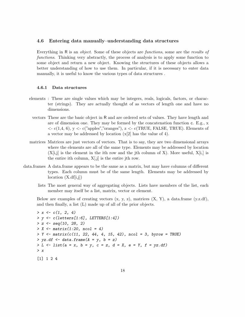
Everything in R is an object. Some of these objects are functions, some are the results offunctions. Thinking very abstractly, the process of analysis is to apply some function tosome object and return a new object. Knowing the structures of these objects allows abetter understanding of how to use them. In particular, if it is necessary to enter datamanually, it is useful to know the various types of data structures .
4.6.1 Data structures
elements : These are single values which may be integers, reals, logicals, factors, or charac-ter (strings). They are actually thought of as vectors of length one and have nodimensions.
vectors These are the basic object in R and are ordered sets of values. They have length andare of dimension one. They may be formed by the concatenation function c. E.g., x<- c(1,4, 6), y <- c(”apples”,”oranges”), z <- c(TRUE, FALSE, TRUE). Elements ofa vector may be addressed by location (x[2] has the value of 4).
matrices Matrices are just vectors of vectors. That is to say, they are two dimensional arrayswhere the elements are all of the same type. Elements may be addressed by location(X[i,j] is the element in the ith row and the jth column of X). More useful, X[i,] isthe entire ith column, X[,j] is the entire jth row.
data.frames A data.frame appears to be the same as a matrix, but may have columns of differenttypes. Each column must be of the same length. Elements may be addressed bylocation (X.df[i,j])
lists The most general way of aggregating objects. Lists have members of the list, eachmember may itself be a list, matrix, vector or element.
Below are examples of creating vectors (x, y, z), matrices (X, Y), a data.frame (y.z.df),and then finally, a list (L) made up of all of the prior objects.
1 a 102 b 123 c 144 d 165 e 186 f 207 A 228 B 249 C 2610 D 28
Thinking analogically, the data.frame is the most similar to the standard spreadsheet wayof organizing data, and most statistical analysis will make use of data.frames or of matrices.The list structure is a particularly appealing way of storing the results of any particularanalysis, for it can hold different types of information as one, high level, object.
If you do know, or can remember the structure of a particular object, then the str functionwill retrieve it for you. This is particularly useful when running a complex statisticalanalysis, for only some results will be shown, even though far more information is hiddenin the object.
> str(L)
List of 6$ a: num [1:3] 1 2 4$ b: chr [1:10] "a" "b" "c" "d" ...
A data.frame is just a collection of objects, each of the same length where subjects arerows and variables are columns. Thus, an experiment might have one or more conditionvariables, and one or more outcome variables. Consider a simple example of two conditions(control vs. experimental) and a measured variable.
> condition = c("e", "e", "e", "c", "c", "c")
> result <- c(2, 3, 4, 1, 2, 3)
> my.data <- data.frame(condition, result)
> my.data
condition result1 e 22 e 33 e 44 c 15 c 26 c 3
4.7 Basic data manipulation
As one would expect, data can be selected, recoded, sorted, and merged using the appro-priate commands.
4.7.1 Editing the data in a data.frame
To change just one or two values in small data frame or matrix, use the functions editand fix.
x <- edit(my.data) #will open an edit window and allow changes, which are then put into x, keeping the old version in my.data
fix(my.data) #immediately changes my.data.
21
4.7.2 Modifying particular cases by a formula
An alternative to using the edit or fix functions is to operate on the data directly. Con-sider the data.frame my.data. Select those cases for which condition is equal to “e” andincrease the values by 2
This ability to manipulate data that meet certain logical conditions is very powerful, forit can be done to turn particular observations into missing data (NA), or to select justcertain cases.
4.7.3 Selecting particular cases or conditions
Just as one can modify certain cases that meet certain conditions, so can one select justthose cases for a new object.
A frequently asked question is how to sort the data file according to some criterion. Con-sider the data.frame, people, made up of names and numbers. The order of names canbe found by the order function, and then a new data.frame can be created using theseorders.
names numbers1 Roger 92 Ellen 103 Anne 324 Mary 355 Carolyn 39
> sorted <- people[order(people$names), ]
> sorted
names numbers3 Anne 325 Carolyn 392 Ellen 104 Mary 351 Roger 9
4.7.5 Merging two data.frames
Suppose we have another data.frame, gender, that catalogs the genders of the same people.To merge these two data.frames together, use the merge function specifying the variableto use to combine the two data.frames.
names gender1 Roger M2 Ellen F3 Anne F4 Mary F5 Carolyn F
> merge(gender, people, by = "names")
names gender numbers1 Anne F 32
23
2 Carolyn F 393 Ellen F 104 Mary F 355 Roger M 9
Using this technique, we routinely merge data files of 40-60,000 records with 300 variableswith other files with 100 variables.
5 Basic descriptive statistics
Basic descriptive statistics are most easily reported by using the summary, mean and Stan-dard Deviations (sd) commands. Using the describe function available in the psychpackage produces output more useful to most psychologists. Graphical displays that alsocapture the data are available as a boxplot.
> describe(my.data)
var n mean sd median trimmed mad min max range skew kurtosis secondition* 1 6 1.5 0.55 1.5 1.5 0.74 1 2 1 0 -2.31 0.22result 2 6 3.5 1.87 3.5 3.5 2.22 1 6 5 0 -1.80 0.76
It is sometimes useful to report statistics by a particular group. This can be done using thedescribe.by function. We use a different data set sat.act which has self reported SATVerbal, Quant and ACT scores for 700 participants collected on the personality-project.orgweb site. In addition, we have gender, education and age. The first describe is for all thecases, the second is broken down by gender (males=1, females=2). To make the outputshorter, the option to not show the skews and kurtosi is set.
describe.by is just an example of a more basic R function, by. As can be seen in the helppage for by, an alternative way to do the preceding analysis is just
6 Day 2: Graphical data displays and Exploratory DataAnalysis
A compelling reason to use R is for its graphics capabilities. There are at least threedifferent graphics options available, only one of which, base graphics will be discussedhere. The others are lattice graphics and ggobi (based upon the grammar of graphicsWilkinson.
Although not all threats to inference can be detected graphically, one of the most powerfulstatistical tests for non-linearity and outliers is the well known but not often used “inter-occular trauma test”. A classic example of the need to examine one’s data for the effect ofnon-linearity and the effect of outliers is the data set of Anscombe (1973) which is includedas the data(anscombe) data set. The data set is striking for it shows four patterns ofresults, with equal regressions and equal descriptive statistics. The graphs differ drasticallyin appearance for one actually has a curvilinear relationship, two have one extreme score,and one shows the expected pattern. Anscombe’s discussion of the importance of graphsis just as timely now as it was 35 years ago:
Graphs can have various purposes, such as (i) to help us perceive and appreciatesome broad features of the data, (ii) to let us look behind these broad featuresand see what else is there. Most kinds of statistical calculaton rest on assump-tions about the behavior of the data. Those assumptions may be false, and thecalculations may be misleading. We ought always to try to check whether theassumptions are reasonably correct; and if they are wrong we ought to be ableto perceive in what ways the are wrong. Graphs are very valuable for thesepurposes. (Anscombe, 1973, p 17).
6.1 The Scatter Plot Matrix (SPLOM)
The problem with suggesting looking at scatter plots of the data is the number of suchplots grows by the square of the number of variables. A solution is the scatter plot matrix(SPLOM) available in the pairs.panels function which is based upon the pairs func-tion. pairs.panels show the all the pairwise relationships, as well as histograms of theindividual variables. Additional output includes the Pearson Product Moment CorrelationCoefficient , the locally weighted polynomial regression (LOWESS), and a density curve foreach variable (Figure 5). This kind of graph is particularly useful for less than about 10variables. Students in an introductory methods course do not seem to realize that this isunusual way of plotting data.
26
> data(sat.act)
> pairs.panels(sat.act)
gender
0 2 4
0.09 −0.02
5 15 30
−0.04 −0.02
200 500 800
1.0
1.4
1.8
−0.17
02
4
●●●
●
●
● ●
●
●
●
●
●● ●
●
●
●
●● ●
●
●
●
●●
●
●
●
●●
●
●●
●●
●
●
●
●
●
● ●
●●●
●
●● ●
●
● ●●
●
●● ●
●
●
●
●●
●
●
●
●
●
●●
●
●
●
●
●
●
●
●●
●
●
●
●● ●●●●
●
●
●
●
●
●● ●
●●
●
●
●
●
● ●
● ●
●
●
●
●
● ●
●
● ●●
●
●
●
●
●● ●
●
●
● ●
●●●
●
●
●●
●●
●●●
●
●
●
●●●●
●●●
●
●● ●●
●
●●
●
●
●
●● ●
●
●
●●
●
● ●●
●
●
●
●
●●
●
●
●●
●
●
● ●
●
●
●
● ●
●
●
● ●●
●
●
●
●
●
●●
● ●
● ●
●
●●●
●
●
●
●●
●
●
●
●
●
●●
●●
●●
●
●
●
●
●
●
● ●
●
●
●
●
●
●● ●
●
●
●
●
●
●●●
●
●●●●●●●
● ●
●
●
●●
●●●
●
●
●
●●
●
●●●●
●
●
●●
●●
●●
● ●
●
●●
●
● ●
●
●
●
●
●
●
●
●
●●
●●
●
●
●
●
●
●
●
●●●
●
●
●●
●
●
●●
●
●
●
●●
●
●
●
●
●●
●
●
●
●
● ●
●
●
●
●
●●
●
●●
●
●
●
●●●●
●
●
●
●●
● ●
●
●●
●
●●●
●
●● ●●●●●
●
●
●
●
●
●●●
●●
●●●●
●
●●
●
●
●
●
●
●
●●
●
●
●●
●
●
●
●
●
● ●
●
●
●
●
●●
●
●
●
●
●
●
●●
●
●●●●
●
●
●
●●●
●●
●●
●
●● ●
●
●
●
●
●● ●
●
● ●●●
●
●
●
●
●
●
●
●
●●
●
●
●●●●
●
●
●
●●●
●●
●
●
●
●
● ●
●
●
●
●
●●●
●
●
●●
●
●
●●
●
●
●● ●● ●●
●
●
●
●●
●
●●
●
●
● ●
●
●
●●
●
●●●
●
●
●
●
●
●
●
●
●
●
●
●
●
●
●
●●
●●●●
●
●
●
●
●
●
●
●
●
●
●
●● ●●
●
●●● ●●● ●●●
●
●● ●●●●●
●
●●● ●●●●●● ●●
●
●●●●●
●●
●
●
●●
●
●●
●
●●
●
●
●
●●●
●●
●
●
●
●
●
●
●
●
●
●●
●● ●●●●
●
●
●
●●
●
●
●●
●
●
●
●● ●
●●
●
●
●
●
●●
●●
●●
●
●●
●
●●
●
●
●●●
●
●
●●
●
●
●● ●
●
●
●
●●
●
●●●
●
●
●
●
●
education
0.55 0.15 0.05 0.03
●●●
●
●
●●
●●
●
●
●●
●
●●
●
●
●
●
●
●
●
●
●
●
●●
●●
●
●●●
●
●
●
●
●
●
●●
●
●
●
●
●●
●
●
●
●●●●
●●●
●
●
●
●
●●
●
●
●
●
●
●●●
●
●
●
●
●
●
●
●●
●
●●
●
●
●
●●
●
●●
●●
●
●
●
●
●●
●
● ●● ●●
●
●
●
●
●
●
●
●●●
●
●●●
●●
●
●
●●
●●●
●
●
●●
●
●
●●
●
●
●
●
●●●●
●
●
●
●
●● ●●
●
●● ●
●●●●
●
●●
●
●
●
●
●
●
●
●●●
●●
●
●
●
●
●●
●
●
●
●
●
●
●
●
●
●●●●●
●
●
●●
●
●
●
●
●
●
●●●
●●
●●● ●●
●
●
●
●●
●
●
●●●
●●
●
●
●
●
●
●
●● ●
●
●● ●
●
●
●
●
●●●● ●
●●●
●
●●
●
● ●
●
●
●●
●
●
●●
●
●
●
●
●
●●
●
●
●●●●
●●●●● ●
●●●
●
●
●●●
●●
●
●
●
●
●
●
●●
●
●
●
●
●
●
●
●●●
●
●
●
●
●
●●
●●●
●
●●
●
●●
●
●
●
●●
●
●
● ●
●●
●
●
●●
●
●●
●
●
●
●●●●
●
●●
●
●
●
●
●
●●●
●●●●●●●●●●●
●●
●
●
●
●●
●
●
●
●
●
●●
●
●●
●●
●
●
●
●
●
●
●
●
●●
●
●
●
●
●●
●●●
●
●●●●●●●●
●
●●
●
●●●●
●
●● ●●●●●
●●
●
●
●
●
●
●
●
●●● ●●● ●●●
●
●
●
●●
●
●
●
●● ●●
●●
●●●●
●
●●●●●
●
●
●●● ●●
●
●
●
●●●
●
●●●●
●
●●●●
●● ●● ●●
●
●
● ●●
●
●●
●●
●
●●
● ●●
●
●●●●
●●
●
●●
●
●
●
●
●● ●●
●
●● ●●●●
●●●●
●
●
●
●
●
●● ●●●●●●●● ●●● ●●●●
●● ●●●●● ●●●● ●●●●●● ●●●●●●●
●
●
●
●●
●
●●
●
●
●
●●
●
●
●
●●
●●●
●●
●
●
●
●
●
●●
●
●
●●
●●●●
●
●●
●●●
●
●●
●
●●
●
● ●
●●
●
●●
●●●
●●
●●
●
●
●
●
●
● ●
●
●
●●
●
●
●
●
●
●
●●
●●
●
●●
●
●●
●
●
●
●
●
● ●●●●
●
●
●●
●●
●
●
●●
●
●●
●
●
●
●
●
●
●
●
●
●
●●
●●
●
●● ●
●
●
●
●
●
●
●●
●
●
●
●
●●●
●
●
●●●
●
●●
●
●
●
●
●
●●
●
●
●
●
●
●● ●
●
●
●
●
●
●
●
●●
●
●●
●
●
●
●●
●
●●
●●
●
●
●
●
●●
●
●● ●●●
●
●
●
●
●
●
●
●●
●
●
●●
●●●
●
●
●●
●●●
●
●
●●
●
●
●●
●
●
●
●
●●●●
●
●
●
●
●●●●
●
●●●
●●●●
●
●●
●
●
●
●
●
●
●
●● ●
●●
●
●
●
●
●●
●
●
●
●
●
●
●
●
●
●●● ●●
●
●
●●
●
●
●
●
●
●
●●●
●●
● ●●● ●
●
●
●
●●
●
●
●●
●● ●
●
●
●
●
●
●
●● ●
●
●●●
●
●
●
●
●●●●●
●●●
●
●●
●
●●
●
●
●●
●
●
●●
●
●
●
●
●
●●
●
●
●●●●
●●
●●●●
●●●
●
●
●●
●
●●
●
●
●
●
●
●
●●
●
●
●
●
●
●
●
●●●
●
●
●
●
●
●●●
● ●
●
●●
●
●●
●
●
●
●●
●
●
●●
●●
●
●
●●
●
●●
●
●
●
●●●●
●
●●
●
●
●
●
●
●● ●
●●●●
●●●●●●●
●●
●
●
●
●●
●
●
●
●
●
●●
●
●●
●●
●
●
●
●
●
●
●
●
●●
●
●
●
●
●●
●● ●
●
●●● ●●●●
●
●
●●
●
●●●●
●
●● ●●●●●
●●
●
●
●
●
●
●
●
●●●●● ●●●●
●
●
●
●●
●
●
●
●●●●
●●
●●
●●
●
●●●●●
●
●
●● ●●●
●
●
●
●●●
●
● ●●●
●
●●●●
●●●●●●
●
●
●●●
●
●●
●●
●
●●
● ●●
●
●●●●
●●
●
●●
●
●
●
●
●● ●●
●
●● ●●●●
●●
●●●
●
●
●
●
●● ●●●●● ●●●●●●●●●●
●●●●●●●●●●●●●●●●●●●
●●●●●
●
●
●
●●
●
●●
●
●
●
●●
●
●
●
●●
●●●
●●
●
●
●
●
●
●●
●
●
●●
●●●●
●
●●
●●●
●
●●
●
●●
●
●●
●●
●
●●
●●●
●●
●●
●
●
●
●
●
●●
●
●
●●
●
●
●
●
●
●
●●
● ●
●
●●
●
● ●
●
●
●
●
●
●●
age
0.11 −0.04
2040
60
−0.03
515
30
●
●
●
●
●
●
●
● ●
●
●
●
●
●
●●
●●
●
●
●●●●●● ●
●
●
●
●
●
●
●●
●●
●
●
●
● ●●
●●
●
●
●
●
●●
●●
●●
●
●
●
●
●●●
●●
●
●
●
●●
●●
● ●
● ●
●●
●
●
●
●●
●
●●
●
●
●● ●●
●
●●
●
●
●
●
●●
●
● ●
● ●
●
●●
●
● ●●●
●
●
●
●●
●
●
●
●
●
●
● ●●
●
●
●
●
●
●●
●
●●
●●
●
●
●
●
●●●
●
●
●
●
●
●
● ●
●
●
●
●
●
●
●
●●
●
●
● ●
●
●●
●
●
●
●●
●
●
●●●
●●●
●
●● ●●
●●
●
●
●
●
●
● ●●●●●● ●
● ●●
●
●
●
●
●●●
●
●●
●
●
●
●●
●
●
●
●
●
●
●
●
●
●●●● ●
● ●
●●●
●●
●
●
●
●●
●
●
●
●
●
●
●
●
●●●
●
●
●
●●
●
●●●● ●
●
●
●
●
●
●
●
●
●
●●
●●●
●
●
●●
●
●●
●●
●
●●
●
●
●
●
●●●
●
●
●
●
●
●
●●●●●
●
●
●●
●●
●
●●
●
●
●
●
●
●
●
●
●
●
●●
●
●●
●●
●
●
●
●
●
●
●●
●
●
●
●
●
●
●
●
●●
●
●
●●
●●●●
●●●
●
●
●●●
●●●
●
●●
●●
●
●
●
●
●
●
●
●●●
●
●
●
●
●●● ●
●●
●
●
●
●
●●
●
●
●
●
●
●
●
●
● ●
●●●
●●
●
●
●●●●
●●
●
●
● ●
● ●
●
●
●
●
●●
●●
●
●
●
●
●● ●
●
●
●
●
●
●
● ●
●
●
●
●●
●
●●
●
●
●
●●
●
●
●
●
●
●●
●
●
●●
●
●
●
● ●●
●
●
●
●●●
●
●
●
●
●
●
●●
●
●●
●●
●●
●
●
●
● ●
●
●
●
●●
●●
●
●
●
●
●
●
●
●●
●
●
●
●
●
●●●●
●
●●
●
●●
●
●
●●
●
●
●●●
●
●
●
●●
●
●
● ●
●
●●●
●●
●●
●
●
●●
●●●● ●
●
●
●
●
●●●
●
●●●●●
● ●●
●
●
●●
●●
●
● ●
●●●●
●
●●●
●●
●
●
●
●
●●
●
●
●●
●
●
●
●
●
●
●
●
●●
●●
●
●
●
●
●
●●
●●●●
●
●●●
●
●●
●
●
●●●●●
●
●●
●
●●
●
● ●
●
●
● ●
●
● ●
●
●●●●
●
● ●
●
●●●
● ●●●
●
●
●●
●●
●
●
●
●
●
●
●
● ●
●
●
●
●
●
● ●
● ●
●
●
●●● ●●●●
●
●
●
●
●
●
●●
●●
●
●
●
●●●
●●
●
●
●
●
●●
●●
●●
●
●
●
●
● ●●
●●
●
●
●
●●
●●
● ●
● ●
●●
●
●
●
● ●
●
●●
●
●
● ●●●
●
●●
●
●
●
●
●●
●
●●
●●
●
●●
●
●●●
●
●
●
●
●●
●
●
●
●
●
●
●●●
●
●
●
●
●
●●
●
●●
●●
●
●
●
●
●●●
●
●
●
●
●
●
● ●
●
●
●
●
●
●
●
● ●
●
●
●●
●
●●
●
●
●
●●
●
●
●●●
●● ●
●
● ●● ●
●●
●
●
●
●
●
●● ● ●●● ●●●●
●
●
●
●
●
●●
●
●
●●
●
●
●
●●
●
●
●
●
●
●
●
●
●
●●● ●●
● ●
●●●
● ●
●
●
●
●●
●
●
●
●
●
●
●
●
●●●
●
●
●
●●
●
●●
●● ●
●
●
●
●
●
●
●
●
●
●●
●● ●
●
●
● ●
●
●●
●●
●
● ●
●
●
●
●
● ●●
●
●
●
●
●
●
●● ●
●●
●
●
● ●
●●
●
●●
●
●
●
●
●
●
●
●
●
●
●●
●
● ●
●●
●
●
●
●
●
●
● ●
●
●
●
●
●
●
●
●
●●
●
●
●●
● ●●●
●●●
●
●
●●●
●●●
●
●●
●●
●
●
●
●
●
●
●
●●●
●
●
●
●
●● ●●
●●
●
●
●
●
●●
●
●
●
●
●
●
●
●
●●
●● ●
●●
●
●
●●●●
●●
●
●
●●
● ●
●
●
●
●
●●
●●
●
●
●
●
●● ●
●
●
●
●
●
●
● ●
●
●
●
●●
●
● ●
●
●
●
●●
●
●
●
●
●
●●
●
●
●●
●
●
●
●●●
●
●
●
●●●
●
●
●
●
●
●
●●
●
●●
●●●●
●
●
●
●●
●
●
●
●●
● ●
●
●
●
●
●
●
●
●●
●
●
●
●
●
●●● ●
●
●●
●
●●
●
●
●●
●
●
●●
●
●
●
●
● ●
●
●
● ●
●
●●●
●●
●●
●
●
●●
●●●●●
●
●
●
●
●●●●
●●●●●
●●●
●
●
●●
●●
●
●●
●●● ●
●
●●
●
● ●
●
●
●
●
●●
●
●
●●
●
●
●
●
●
●
●
●
●●
●●
●
●
●
●
●
●●
●●●●
●
●●●
●
●●
●
●
●●●●●
●
●●
●
●●●
● ●
●
●
● ●
●
●●
●
●●● ●
●
●●
●
● ● ●
●● ●●
●
●
● ●
●●
●
●
●
●
●
●
●
● ●
●
●
●
●
●
● ●
● ●
●
●
●●● ●●● ●
●
●
●
●
●
●
●●
● ●
●
●
●
●● ●
● ●
●
●
●
●
●●
●●
●●
●
●
●
●
● ●●
●●
●
●
●
● ●
●●
● ●
●●
● ●
●
●
●
●●
●
●●
●
●
● ● ●●
●
●●
●
●
●
●
●●
●
●●
●●
●
●●
●
●●●
●
●
●
●
●●
●
●
●
●
●
●
●●●
●
●
●
●
●
●●
●
●●
●●
●
●
●
●
●●●
●
●
●
●
●
●
● ●
●
●
●
●
●
●
●
●●
●
●
●●
●
●●
●
●
●
●●
●
●
●●●
●● ●
●
● ●● ●
●●
●
●
●
●
●
● ●● ●●● ●●
● ●●
●
●
●
●
●●●
●
●●
●
●
●
●●
●
●
●
●
●
●
●
●
●
● ●● ●●
●●
●●●
● ●
●
●
●
●●
●
●
●
●
●
●
●
●
● ●●
●
●
●
●●
●
●●●● ●
●
●
●
●
●
●
●
●
●
●●
●●●
●
●
●●
●
●●
●●
●
● ●
●
●
●
●
● ●●
●
●
●
●
●
●
●● ●
●●
●
●
● ●
●●
●
●●
●
●
●
●
●
●
●
●
●
●
●●
●
● ●
●●
●
●
●
●
●
●
●●
●
●
●
●
●
●
●
●
●●
●
●
●●
● ●●●
●●●
●
●
●●●
●●●
●
●●
●●
●
●
●
●
●
●
●
●●●
●
●
●
●
●● ●●
●●
●
●
●
●
●●
●
●
●
●
●
●
●
●
●●
●●●
●●
●
●
●●●●
●●
●
●
●●
●●
●
●
●
●
●●
●●
●
●
●
●
●●●
●
●
●
●
●
●
● ●
●
●
●
●●
●
●●
●
●
●
●●
●
●
●
●
●
●●
●
●
●●
●
●
●
●●●
●
●
●
●●●
●
●
●
●
●
●
●●
●
●●
●●●●
●
●
●
●●
●
●
●
●●
●●
●
●
●
●
●
●
●
●●
●
●
●
●
●
●●● ●
●
●●
●
●●
●
●
●●
●
●
●●●
●
●
●
●●
●
●
●●
●
●●●
●●
●●
●
●
●●
●●●●●
●
●
●
●
●●
●●
●●●●●
●●●
●
●
●●
● ●
●
●●
● ●●●
●
●●
●
● ●
●
●
●
●
●●
●
●
●●
●
●
●
●
●
●
●
●
●●
●●
●
●
●
●
●
●●
●●●●
●
●●●
●
●●
●
●
●●●●●
●
●●
●
●●
●
● ●
●
●
● ●
●
●●
●
● ●● ●
●
● ●
●
● ●●
●●●●
●
●
● ●
●● ACT
0.56 0.59
●
●
●
●●●
●
●
●
●●
●
●
●
●●●
●
●●●●
●
●
●
● ●
●
●
●
●●●
●●
●
●
●●
●
●
●
●●
●
●
●
●
●
●
● ●
●●
●
●
●
●
●
●
●
●●●
● ●
●
●●●
●
●
●● ●
●
●
●
●
●
●
●
●
●●●
●
●
●
●
●
●
●
●
●
●
●
●
●
●
●
●
●
●
●●
●
●
●● ●
●
●●●●●
●
●●
●
●
●
●
●●●
●
●●
●●
●
●
●
●
●
●
●●
●
●
●
●●
●
●
●
●
●●
●
●
●●
●
●
●
●●
●
●
●
●●
●
●●
●●●●
●●
●
●
●
●
●
●●
●
●
●●
● ●● ●
●
●
●●
●
●●
●●●●
●
●
●
●●
●
●●
●
●●
●
●
●
●
●
●
●
●
●
●●
●
●
●
●●
●
●
●
●● ●●
●●
●
●
●● ●●
●
●
●
●●
●
●
●
●
●●
●
●
●
●
●
●
●●
●
●●
●
●●●
●
●●
●
●
●
●●●
●
●
●
●
●
●
●
●
●
●
●●
●
●
●●
●●●
●
●●
●●
●●●
●
●
●
●
●
●
●
●
●
●
●
●
●
●
●
●
●● ●
●
●
●
●●
●●●
●
●
●
●
●
●●●●
●
●● ●
●
●
●●
●
●
●
●●
●●
●●
●
●
●
●●
●
●
●
●●●
●
●
●● ●
●
●
●
●
●
●
●●
●
●
●●
●
●
●
●
●
●
●●
●
●●●
●
●
●●
●●
●
●●
●
●
●
●
●● ●
●
●● ●
●
●
●●
●
●
●
●
●
●●●●
●
●●
●
●
●
●
●
●
●
●
●
●●●
●●
● ●
●
●
● ●●
●
●
●●●●
●
●
●
●
●
●
●●
●
●●●
●
●●
●●
●
●
●
●●●
●
●
●
●●●
●
●
●
●
●
●
●
●●
●
●
●
●●
●
●
●
●●● ●
●
●
●
●●●
●
●●
●
●●
●
●●
●
●●●
●●
●
●● ●
●
●●●●●
●
●●
●
●●
●
●●
●
●
●
●●
●
●
● ●
●
●
●
●●
●
●
●●●●● ●●
●
●
●●
●●
● ●
●
●●●
●●
●
●
●
●
●●
●
●
●
● ●●●●●
●●
●
●●●
●
●
●
●
●
●
●
●
●
●
●●●●
●
●
● ●
●●
●
●
●
●
●
●
●●
●●
●
●●
●
●●●
●
●
●
●
●●
●
●
●
●
●
●
●
●
●
●●●
●
●●●
●
●
●
●
●●
●
●
●
●
●●
●
●●
●
●
●
●
●●●●
●
●
●
●
●
●
●
●●
● ●●
●
●
●●
●●
●
●
●●
●
●
●
● ●●
●
●●● ●
●
●
●
●●
●
●
●
● ●●
●●
●
●
●●
●
●
●
●●
●
●
●
●
●
●
●●
● ●
●
●
●
●
●
●
●
●● ●
● ●
●
●●
●
●
●
●● ●
●
●
●
●
●
●
●
●
●●●
●
●
●
●
●
●
●
●
●
●
●
●
●
●
●
●
●
●
●●
●
●
●●●
●
●●●
●●
●
●●
●
●
●
●
●●
●
●
●●
●●
●
●
●
●
●
●
●●
●
●
●
●●
●
●
●
●
●●
●
●
●●
●
●
●
●●
●
●
●
● ●
●
● ●
●●● ●
● ●
●
●
●
●
●
●●
●
●
●●
●●●●
●
●
●●
●
●●
●● ●
●
●
●
●
●●
●
●●
●
●●
●
●
●
●
●
●
●
●
●
●●
●
●
●
●●
●
●
●
●●● ●
●●
●
●
●●●
●
●
●
●
●●
●
●
●
●
●●
●
●
●
●
●
●
●●
●
● ●
●
●●●
●
●●
●
●
●
●●
●
●
●
●
●
●
●
●
●
●
●
●●
●
●
●●
●●
●
●
●●
●●
●●●
●
●
●
●
●
●
●
●
●
●
●
●
●
●
●
●
●●●
●
●
●
● ●
●● ●
●
●
●
●
●
●●● ●
●
● ●●
●
●
●●
●
●
●
●●
●●
●●
●
●
●
●●
●
●
●
●●●
●
●
●●●
●
●
●
●
●
●
●●
●
●
●●
●
●
●
●
●
●
●●
●
●●
●
●
●
●●
● ●
●
●●
●
●
●
●
●●●
●
●●●
●
●
●●
●
●
●
●
●
●●
●●
●
●●
●
●
●
●
●
●
●
●
●
●●●
●●
● ●
●
●
●●●
●
●
●●●
●
●
●
●
●
●
●
●●
●
●●●
●
●●
●●
●
●
●
●●●
●
●
●
●●●
●
●
●
●
●
●
●
● ●
●
●
●
●●
●
●
●
●●●●
●
●
●
●●●
●
●●
●
● ●
●
●●
●
●●
●
●●
●
●● ●
●
●●
●●
●
●
●●
●
●●
●
●●
●
●
●
●●
●
●
●●
●
●
●
●●
●
●
●●●●●●●
●
●
●●
●●
●●
●
●●●
●●
●
●
●
●
●●
●
●
●
● ●●●●●
●●
●
●●
●
●
●
●
●
●
●
●
●
●
●
●●●●
●
●
● ●
●●
●
●
●
●
●
●
●●
●●●
● ●
●
●●●
●
●
●
●
●●
●
●
●
●
●
●
●
●
●
●●●
●
●●●
●
●
●
●
●●
●
●
●
●
●●
●
●●
●
●
●
●
● ●● ●
●
●
●
●
●
●
●
● ●
●●●
●
●
●●
●●
●
●
●●
●
●
●
● ●●
●
●● ●●
●
●
●
● ●
●
●
●
● ●●
●●
●
●
●●
●
●
●
●●
●
●
●
●
●
●
●●
● ●
●
●
●
●
●
●
●
●●●
● ●
●
●●
●
●
●
●●●
●
●
●
●
●
●
●
●
● ●●
●
●
●
●
●
●
●
●
●
●
●
●
●
●
●
●
●
●
●●
●
●
●●●
●
●●●●
●
●
●●
●
●
●
●
●●
●
●
●●
●●
●
●
●
●
●
●
●●
●
●
●
●●
●
●
●
●
●●
●
●
●●
●
●
●
●●
●
●
●
● ●
●
● ●
●●● ●
●●
●
●
●
●
●
●●
●
●
●●
●●●●
●
●
●●
●
●●
●● ●
●
●
●
●
●●
●
●●
●
●●
●
●
●
●
●
●
●
●
●
●●
●
●
●
●●
●
●
●
● ●● ●
●●
●
●
●●●
●
●
●
●
●●
●
●
●
●
●●
●
●
●
●
●
●
● ●
●
● ●
●
●●●
●
●●
●
●
●
●●
●
●
●
●
●
●
●
●
●
●
●
●●
●
●
●●
●●●
●
●●
●●
●●●
●
●
●
●
●
●
●
●
●
●
●
●
●
●
●
●
●●●
●
●
●
● ●
●● ●
●
●
●
●
●
●●● ●
●
● ●●
●
●
●●
●
●
●
●●
●●
●●
●
●
●
●●
●
●
●
●●●
●
●
●●●
●
●
●
●
●
●
●●
●
●
●●
●
●
●
●
●
●
●●
●
●●
●
●
●
●●
●●
●
●●
●
●
●
●
●●●
●
●●●
●
●
●●
●
●
●
●
●
●●
●●
●
●●
●
●
●
●
●
●
●
●
●
●● ●
●●
● ●
●
●
●●●
●
●
●●●
●
●
●
●
●
●
●
●●
●
●●●
●
●●
●●
●
●
●
●●●
●
●
●
●●●
●
●
●
●
●
●
●
●●
●
●
●
●●
●
●
●
●●●●
●
●
●
●●●
●
●●
●
●●
●
●●
●
●●
●
●●
●
●● ●
●
●●
●●
●
●
●●
●
●●
●
●●
●
●
●
●●
●
●
●●
●
●
●
●●
●
●
●●●●●●●
●
●
●●
●●
●●
●
●●●
●●
●
●
●
●
●●
●
●
●
● ●●●●●
●●
●
●●
●
●
●
●
●
●
●
●
●
●
●
●●●●
●
●
● ●
●●
●
●
●
●
●
●
●●
●●●
● ●
●
●●●
●
●
●
●
●●
●
●
●
●
●
●
●
●
●
●●●
●
●● ●
●
●
●
●
●●●
●
●
●
●●
●
●●
●
●
●
●
●●● ●
●
●
●
●
●
●
●
● ●
●●●
●
●
●●
●●
●
●
●●
●
●
●
●● ●
●
●●●●
●
●
●
●●
●
●
●
●● ●
●●
●
●
● ●
●
●
●
●●
●
●
●
●
●
●
●●
● ●
●
●
●
●
●
●
●
●●●
● ●
●
●●
●
●
●
●●●
●
●
●
●
●
●
●
●
●●●
●
●
●
●
●
●
●
●
●
●
●
●
●
●
●
●
●
●
● ●
●
●
●●●
●
●● ●
●●
●
●●
●
●
●
●
●●●
●
●●
●●
●
●
●
●
●
●
●●
●
●
●
●●
●
●
●
●
●●
●
●
●●
●
●
●
●●
●
●
●
● ●
●
● ●
●●●●
● ●
●
●
●
●
●
●●
●
●
●●
●●● ●
●
●
●●
●
●●●
●●●
●
●
●
●●
●
●●
●
●●
●
●
●
●
●
●
●
●
●
●●
●
●
●
●●
●
●
●
●●●●
● ●
●
●
●● ●
●
●
●
●
●●
●
●
●
●
●●
●
●
●
●
●
●
● ●
●
●●
●
●●●
●
●●
●
●
●
●●
●
●
●
●
●
●
●
●
●
●
●
● ●
●
●
●●
●●
●
●
●●
●●
●●●
●
●
●
●
●
●
●
●
●
●
●
●
●
●
●
●
●●●
●
●
●
●●
● ●●
●
●
●
●
●
●●●●
●
● ●●
●
●
● ●
●
●
●
● ●
●●
●●
●
●
●
●●
●
●
●
●●●
●
●
●●●
●
●
●
●
●
●
●●
●
●
●●
●
●
●
●
●
●
●●
●
●●
●
●
●
●●
●●
●
● ●
●
●
●
●
●● ●
●
●●●
●
●
● ●
●
●
●
●
●
●●
●●
●
●●
●
●
●
●
●
●
●
●
●
●●●
●●
● ●
●
●
●●●
●
●
● ●●
●
●
●
●
●
●
●
●●
●
●●●
●
●●
●●
●
●
●
●●●
●
●
●
●●●
●
●
●
●
●
●
●
● ●
●
●
●
●●
●
●
●
●●●●
●
●
●
●●
●
●
●●
●
●●
●
●●
●
●●
●
●●
●
●● ●
●
●●●●
●
●
●●
●
● ●
●
●●
●
●
●
●●
●
●
● ●
●
●
●
●●
●
●
●●●
● ●●●
●
●
● ●
●●
●●
●
●●●
●●
●
●
●
●
●●
●
●
●
● ●●●●
●
●●
●
●●●
●
●
●
●
●
●
●
●
●
●
●● ●●
●
●
●●
● ●
●
●
●
●
●
●
●●
●●
●
● ●
●
●●●
●
●
●
●
●●
●
●
●
●
●
●
●
●
●
●●●
●
●●●
●
●
●
●
●●
●
●
●
●
●●
●
●●
●
●
●
●
●●●●
●
●
●
●
●
●
●
●●
●●SATV
200
500
800
0.64
1.0 1.4 1.8
200
500
800
●●●
●●
●
●
●●
●
●
●●
●
●●
●●
●
●
●●
●
●
●
●●
●
●●●
●●
●●●●●●
●
● ●
●
●
●
●
●●
●
●
●
●●
●●●
●●
●
●
●●
●
●
●
●
●
●●●
●
●
●
●●
●●●
●
●●●
●
●●
●
●●
●
●
●● ●
●
●
●
●
●
●
●●
●
●● ●
●●
●
●
●
●●
●
●
●●
●
●
●●●
●
●
●
●
●
●
●
●● ●
●
●
●
●●●
●●●
●
●
●●
●●
●
●
●●
●
●
●●●
●
●
●●
●
●
●●
●● ●●
●● ●
●●●
●
●●
●
●
●●
●
●
●
●
●
●
●●
●●
●
●
●
●
● ●●●
●●
●● ●
●
●●
●●
●
●
●
●
●
●
●● ●
●
●●
●
●
●
●●●●
●
●
●
●
●
●
●●
●●
●
●
●●
●
●
●●
●
●
●
●
●
●
●●●
●
●
●●
●
●
●
●
●
●●
●
●●
● ●
●
●
●
●●
●●
●
●
●
●
●
●
●
●
●
●
●
●●
●
●
●●
●● ●
●
●
●●
●
●
●
●
●
●●
●●●
● ●
●
●
●
●
●●
●
●
●
●
●
●
●
●
●
●
●
●
●
●●
● ●
●
●
●
●
●
●●
●
●
●
●●
●●
●
●
●
●
●
●
●●
●
●●
●
●
●
●
●
●● ●
●●
●
●
●
●
●
●
●
●●
●
●
●
●
●●
●●
●
●
●
●
●
●
●
●●
●
●
●
●
●
●
●
●●
●
●
●●
●
●●
●
● ●
●
●●
●
●
●
●●●●●
●
● ●
●
●
●
●
●●
●
●
●
●●
●●
●●
●
●
●●
●●●
●
●
●●
●
●
●
●●
●
●●●●●
●
●
●●
●●
●
●
●
●
●
●●
●
●●
●
●
●●●
●
●
●●
●
●
●
●●
●
●
●
●
● ●●
●●●
●
●
●●●
●●●
●●
●●
●●
●●●
●
●
●
●
●
●
●
●
●●
●
●
●●
●
●
●
●
●
●
●
●
●
●
● ●
●
●
●
● ●
●
●
●●●●●
●●
● ●●●●●●
●
●
●●
●
●
●
●
●
●
●●●●
●●
●
●
●
●
●
●
●●
●●●
●●
●
●
●
●●
●
●
●
●
●
●
●●●
● ●
●
●●
●
●
●
●
●
●●
●●
●
●
●
●
●●
●●●
●
●
●
●
●●●
●
●
●●●
●●
●
●
●
●
●
●
●
● ●
●
●
●
●
●
●
●●
●
●
●
●
●
●
●
●
●
●
●
●●●
●
● ●
●
● ●●●●
●●
●
●
●●
●
●
●●
●
●●
●●●
●
●●
●
●
●
●●
●
●●●
●●
●●●●
●●
●
●●
●
●
●
●
●●
●
●
●
●●
●●●●●
●
●
●●
●
●
●
●
●
●●●
●
●
●
●●
●●●
●
●● ●
●
●●
●
●●
●
●
●● ●
●
●
●
●
●
●
● ●
●
● ●●
●●
●
●
●
●●
●
●
● ●
●
●
●●●
●
●
●
●
●
●
●
●● ●
●
●
●
●●●
●●●
●
●
●●
●●
●
●
●●
●
●
●●●
●
●
●●
●
●
●●
●●●●
●●●
●● ●
●
●●
●
●
●●
●
●
●
●
●
●
●●
● ●
●
●
●
●
●●●
●
●●
●●●
●
●●
● ●
●
●
●
●
●
●
●● ●
●
● ●
●
●
●
●●
●●
●
●
●
●
●
●
●●
●●
●
●
●●
●
●
●●
●
●
●
●
●
●
●●●
●
●
●●
●
●
●
●
●
●●
●
●●
● ●
●
●
●
●●
●●
●
●
●
●
●
●
●
●
●
●
●
●●
●
●
● ●
●●●
●
●
●●
●
●
●
●
●
●●
●●●
●●
●
●
●
●
●●
●
●
●
●
●
●
●
●
●
●
●
●
●
●●
●●
●
●
●
●
●
●●
●
●
●
●●
●●
●
●
●
●
●
●
● ●
●
●●
●
●
●
●
●
●●●
●●
●
●
●
●
●
●
●
●●
●
●
●
●
●●
●●
●
●
●
●
●
●
●
●●
●
●
●
●
●
●
●
●●
●
●
●●
●
●●
●
● ●
●
●●
●
●
●
●●●● ●
●
● ●
●
●
●
●
●●
●
●
●
●●
●●
●●
●
●
● ●
●●●
●
●
●●
●
●
●
●●
●
●●
●●●
●
●
●●
●●
●
●
●
●
●
●●
●
●●
●
●
●●●
●
●
●●
●
●
●
●●
●
●
●
●
●●●
●●●
●
●
●●●
● ●●
●●●
●
●●
●●●
●
●
●
●
●
●
●
●
●●
●
●
●●
●
●
●
●
●
●
●
●
●
●
●●
●
●
●
● ●
●
●
●●●●●
●●
●●●● ●●●
●
●
●●
●
●
●
●
●
●
●●●●
●●
●
●
●
●
●
●
●●
● ●●
● ●
●
●
●
●●
●
●
●
●
●
●
●●
●
● ●
●
●●
●
●
●
●
●
●●
●●
●
●
●
●
●●
●●●
●
●
●
●
●●●
●
●
●● ●
●●
●
●
●
●
●
●
●
● ●
●
●
●
●
●
●
●●
●
●
●
●
●
●
●
●
●
●
●
●●●
●
●●
●
●●
20 40 60
● ●●
●●
●
●
●●
●
●
●●
●
●●
●●
●
●
●●
●
●
●
●●
●
●●●
●●
● ●● ●●
●
●
●●
●
●
●
●
●●
●
●
●
●●
●●●
●●
●
●
●●
●
●
●
●
●
● ●●
●
●
●
●●
●●●
●
●●●
●
● ●
●
●●
●
●
●●●
●
●
●
●
●
●
● ●
●
●●●
●●
●
●
●
●●
●
●
● ●
●
●
●●●
●
●
●
●
●
●
●
● ●●
●
●
●
●●●
●●●
●
●
●●
●●
●
●
●●
●
●
●●●
●
●
●●
●
●
●●
●●●
●
●●●
●●●
●
●●
●
●
●●
●
●
●
●
●
●
●●
● ●
●
●
●
●
●●●●
●●
●● ●
●
●●
● ●
●
●
●
●
●
●
●● ●
●
● ●
●
●
●
●●●
●
●
●
●
●
●
●
●●
●●
●
●
●●
●
●
●●
●
●
●
●
●
●
●● ●●
●
●●
●
●
●
●
●
●●
●
● ●
●●
●
●
●
●●
●●
●
●
●
●
●
●
●
●
●
●
●
●●
●
●
●●
●●●
●
●
●●
●
●
●
●
●
●●
●●●
●●
●
●
●
●
●●
●
●
●
●
●
●
●
●
●
●
●
●
●
●●
●●
●
●
●
●
●
● ●
●
●
●
●●
●●
●
●
●
●
●
●
●●
●
●●
●
●
●
●
●
●●●
●●
●
●
●
●
●
●
●
●●
●
●
●
●
●●
●●
●
●
●
●
●
●
●
● ●
●
●
●
●
●
●
●
●●
●
●
●●
●
●●
●
●●
●
●●
●
●
●
●●
●● ●
●
●●
●
●
●
●
●●
●
●
●
●●
●●
●●
●
●
●●
●●●
●
●
●●
●
●
●
●●
●
●●
●●●
●
●
●●
●●
●
●
●
●
●
●●
●
●●
●
●
●●●
●
●
●●
●
●
●
●●
●
●
●
●
●●●
●●●
●
●
●●●
●●●
●●●
●
●●
●●●
●
●
●
●
●
●
●
●
●●
●
●
●●
●
●
●
●
●
●
●
●
●
●
●●
●
●
●
●●
●
●
●●●●●
●●
●●●●●●●
●
●
●●
●
●
●
●
●
●
●●●●
●●
●
●
●
●
●
●
●●
●●●
●●
●
●
●
●●
●
●
●
●
●
●
●●
●
● ●
●
●●
●
●
●
●
●
●●
●●
●
●
●
●
●●
●●●
●
●
●
●
● ●●
●
●
●● ●
●●
●
●
●
●
●
●
●
● ●
●
●
●
●
●
●
●●
●
●
●
●
●
●
●
●
●
●
●
●●●
●
●●
●
●●● ●
●●
●
●
●
●●
●
●
●●
●
●●
●●
●
●
●●
●
●
●
●●
●
●●●
● ●
●●●●●
●
●
●●
●
●
●
●
●●
●
●
●
●●
●●●
●●
●
●
●●
●
●
●
●
●
●●●
●
●
●
●●
●● ●
●
●●●
●
●●
●
● ●
●
●
●●●
●
●
●
●
●
●
●●
●
●●●
●●
●
●
●
●●
●
●
●●
●
●
● ●●
●
●
●
●
●
●
●
● ●●
●
●
●
●● ●
●●●
●
●
●●
●●
●
●
●●
●
●
● ●●
●
●
●●
●
●
●●
●●●
●
●●●
●● ●
●
●●
●
●
●●
●
●
●
●
●
●
●●
●●
●
●
●
●
●●●●
●●
●●●
●
●●
● ●
●
●
●
●
●
●
●● ●
●
● ●
●
●
●
●●
●●
●
●
●
●
●
●
●●
●●
●
●
●●
●
●
●●
●
●
●
●
●
●
●●●
●
●
●●
●
●
●
●
●
●●
●
● ●
● ●
●
●
●
●●
●●
●
●
●
●
●
●
●
●
●
●
●
●●
●
●
●●
●● ●
●
●
●●
●
●
●
●
●
●●
●●●
● ●
●
●
●
●
●●
●
●
●
●
●
●
●
●
●
●
●
●
●
●●
●●
●
●
●
●
●
●●
●
●
●
●●
● ●
●
●
●
●
●
●
●●
●
●●
●
●
●
●
●
●●●
●●
●
●
●
●
●
●
●
●●
●
●
●
●
●●
●●
●
●
●
●
●
●
●
● ●
●
●
●
●
●
●
●
●●
●
●
●●
●
●●
●
●●
●
●●
●
●
●
●●
●● ●
●
●●
●
●
●
●
●●
●
●
●
●●
●●
●●
●
●
● ●
● ● ●
●
●
●●
●
●
●
●●
●
●●
●● ●
●
●
●●
●●
●
●
●
●
●
●●
●
●●
●
●
●●
●
●
●
●●
●
●
●
●●
●
●
●
●
●● ●
●●●
●
●
● ●●
●●●
●●
●●
●●
● ●●
●
●
●
●
●
●
●
●
●●
●
●
● ●
●
●
●
●
●
●
●
●
●
●
● ●
●
●
●
●●
●
●
●●●●
●
●●
●●●
●●●●
●
●
●●
●
●
●
●
●
●
●●●●
●●
●
●
●
●
●
●
●●●●
●
●●
●
●
●
●●
●
●
●
●
●
●
●●
●
●●
●
●●
●
●
●
●
●
●●
●●
●
●
●
●
●●
●●●
●
●
●
●
● ●●
●
●
●●●
●●
●
●
●
●
●
●
●
●●
●
●
●
●
●
●
●●
●
●
●
●
●
●
●
●
●
●
●
●●●
●
● ●
●
●●
200 500 800
● ●●
●●
●
●
●●
●
●
●●
●
●●
●●
●
●
●●
●
●
●
●●
●
●●●
●●
● ●●●●●
●
● ●
●
●
●
●
●●
●
●
●
●●
● ●●
● ●
●
●
●●
●
●
●
●
●
●●●
●
●
●
●●
●●●
●
●● ●
●
●●
●
● ●
●
●
●●●
●
●
●
●
●
●
●●
●
●● ●
●●
●
●
●
●●
●
●
●●
●
●
●●●
●
●
●
●
●
●
●
●● ●
●
●
●
●● ●
●●●
●
●
●●
●●
●
●
●●
●
●
●●●
●
●
●●
●
●
●●
●● ●
●
●● ●
●●●
●
●●
●
●
●●
●
●
●
●
●
●
●●
●●
●
●
●
●
●●●
●
●●
●●●
●
●●
●●
●
●
●
●
●
●
●● ●
●
● ●
●
●
●
●●
●●
●
●
●
●
●
●
●●
●●
●
●
●●
●
●
●●
●
●
●
●
●
●
●●●
●
●
●●
●
●
●
●
●
●●
●
● ●
● ●
●
●
●
●●
●●
●
●
●
●
●
●
●
●
●
●
●
●●
●
●
●●
●● ●
●
●
●●
●
●
●
●
●
●●
●●●
● ●
●
●
●
●
●●
●
●
●
●
●
●
●
●
●
●
●
●
●
●●
● ●
●
●
●
●
●
●●
●
●
●
●●
●●
●
●
●
●
●
●
●●
●
●●
●
●
●
●
●
●●●
●●
●
●
●
●
●
●
●
●●
●
●
●
●
● ●
●●
●
●
●
●
●
●
●
● ●
●
●
●
●
●
●
●
●●
●
●
●●
●
●●
●
●●
●
●●
●
●
●
●●
●●●
●
● ●
●
●
●
●
●●
●
●
●
●●
●●
●●
●
●
● ●
● ●●
●
●
●●
●
●
●
●●
●
●●
●●●
●
●
●●
●●
●
●
●
●
●
●●
●
●●
●
●
●●
●
●
●
●●
●
●
●
●●
●
●
●
●
●● ●
●●●
●
●
●●●
●●●
●●
●●
●●
● ●●
●
●
●
●
●
●
●
●
● ●
●
●
●●
●
●
●
●
●
●
●
●
●
●
●●
●
●
●
●●
●
●
●●● ●
●
●●
●●●●●● ●
●
●
●●
●
●
●
●
●
●
●● ●●
●●
●
●
●
●
●
●
●●
●●●
●●
●
●
●
●●
●
●
●
●
●
●
●●
●
●●
●
●●
●
●
●
●
●
●●
●●
●
●
●
●
●●
● ●●
●
●
●
●
●●●
●
●
●● ●
●●
●
●
●
●
●
●
●
● ●
●
●
●
●
●
●
●●
●
●
●
●
●
●
●
●
●
●
●
●● ●
●
● ●
●
●●SATQ
Figure 5: A SPLOM plot is a fast way of detecting non-linearities in the pair wise correla-tions as well as problems with distributions. For each cell below the diagonal, the x axisreflects the column variable, the y axis, the row variable.
27
> data(sat.act)
> pairs.panels(sat.act, scale = TRUE)
gender
0 2 4
0.087 −0.021
5 15 30
−0.037 −0.019
200 500 800
1.0
1.4
1.8
−0.17
02
4
●●●
●
●
● ●
●
●
●
●
●● ●
●
●
●
●● ●
●
●
●
●●
●
●
●
●●
●
●●
●●
●
●
●
●
●
● ●
●●●
●
●● ●
●
● ●●
●
●● ●
●
●
●
●●
●
●
●
●
●
●●
●
●
●
●
●
●
●
●●
●
●
●
●● ●●●●
●
●
●
●
●
●● ●
●●
●
●
●
●
● ●
● ●
●
●
●
●
● ●
●
● ●●
●
●
●
●
●● ●
●
●
● ●
●●●
●
●
●●
●●
●●●
●
●
●
●●●●
●●●
●
●● ●●
●
●●
●
●
●
●● ●
●
●
●●
●
● ●●
●
●
●
●
●●
●
●
●●
●
●
● ●
●
●
●
● ●
●
●
● ●●
●
●
●
●
●
●●
● ●
● ●
●
●●●
●
●
●
●●
●
●
●
●
●
●●
●●
●●
●
●
●
●
●
●
● ●
●
●
●
●
●
●● ●
●
●
●
●
●
●●●
●
●●●●●●●
● ●
●
●
●●
●●●
●
●
●
●●
●
●●●●
●
●
●●
●●
●●
● ●
●
●●
●
● ●
●
●
●
●
●
●
●
●
●●
●●
●
●
●
●
●
●
●
●●●
●
●
●●
●
●
●●
●
●
●
●●
●
●
●
●
●●
●
●
●
●
● ●
●
●
●
●
●●
●
●●
●
●
●
●●●●
●
●
●
●●
● ●
●
●●
●
●●●
●
●● ●●●●●
●
●
●
●
●
●●●
●●
●●●●
●
●●
●
●
●
●
●
●
●●
●
●
●●
●
●
●
●
●
● ●
●
●
●
●
●●
●
●
●
●
●
●
●●
●
●●●●
●
●
●
●●●
●●
●●
●
●● ●
●
●
●
●
●● ●
●
● ●●●
●
●
●
●
●
●
●
●
●●
●
●
●●●●
●
●
●
●●●
●●
●
●
●
●
● ●
●
●
●
●
●●●
●
●
●●
●
●
●●
●
●
●● ●● ●●
●
●
●
●●
●
●●
●
●
● ●
●
●
●●
●
●●●
●
●
●
●
●
●
●
●
●
●
●
●
●
●
●
●●
●●●●
●
●
●
●
●
●
●
●
●
●
●
●● ●●
●
●●● ●●● ●●●
●
●● ●●●●●
●
●●● ●●●●●● ●●
●
●●●●●
●●
●
●
●●
●
●●
●
●●
●
●
●
●●●
●●
●
●
●
●
●
●
●
●
●
●●
●● ●●●●
●
●
●
●●
●
●
●●
●
●
●
●● ●
●●
●
●
●
●
●●
●●
●●
●
●●
●
●●
●
●
●●●
●
●
●●
●
●
●● ●
●
●
●
●●
●
●●●
●
●
●
●
●
education
0.55 0.15 0.046 0.035
●●●
●
●
●●
●●
●
●
●●
●
●●
●
●
●
●
●
●
●
●
●
●
●●
●●
●
●●●
●
●
●
●
●
●
●●
●
●
●
●
●●
●
●
●
●●●●
●●●
●
●
●
●
●●
●
●
●
●
●
●●●
●
●
●
●
●
●
●
●●
●
●●
●
●
●
●●
●
●●
●●
●
●
●
●
●●
●
● ●● ●●
●
●
●
●
●
●
●
●●●
●
●●●
●●
●
●
●●
●●●
●
●
●●
●
●
●●
●
●
●
●
●●●●
●
●
●
●
●● ●●
●
●● ●
●●●●
●
●●
●
●
●
●
●
●
●
●●●
●●
●
●
●
●
●●
●
●
●
●
●
●
●
●
●
●●●●●
●
●
●●
●
●
●
●
●
●
●●●
●●
●●● ●●
●
●
●
●●
●
●
●●●
●●
●
●
●
●
●
●
●● ●
●
●● ●
●
●
●
●
●●●● ●
●●●
●
●●
●
● ●
●
●
●●
●
●
●●
●
●
●
●
●
●●
●
●
●●●●
●●●●● ●
●●●
●
●
●●●
●●
●
●
●
●
●
●
●●
●
●
●
●
●
●
●
●●●
●
●
●
●
●
●●
●●●
●
●●
●
●●
●
●
●
●●
●
●
● ●
●●
●
●
●●
●
●●
●
●
●
●●●●
●
●●
●
●
●
●
●
●●●
●●●●●●●●●●●
●●
●
●
●
●●
●
●
●
●
●
●●
●
●●
●●
●
●
●
●
●
●
●
●
●●
●
●
●
●
●●
●●●
●
●●●●●●●●
●
●●
●
●●●●
●
●● ●●●●●
●●
●
●
●
●
●
●
●
●●● ●●● ●●●
●
●
●
●●
●
●
●
●● ●●
●●
●●●●
●
●●●●●
●
●
●●● ●●
●
●
●
●●●
●
●●●●
●
●●●●
●● ●● ●●
●
●
● ●●
●
●●
●●
●
●●
● ●●
●
●●●●
●●
●
●●
●
●
●
●
●● ●●
●
●● ●●●●
●●●●
●
●
●
●
●
●● ●●●●●●●● ●●● ●●●●
●● ●●●●● ●●●● ●●●●●● ●●●●●●●
●
●
●
●●
●
●●
●
●
●
●●
●
●
●
●●
●●●
●●
●
●
●
●
●
●●
●
●
●●
●●●●
●
●●
●●●
●
●●
●
●●
●
● ●
●●
●
●●
●●●
●●
●●
●
●
●
●
●
● ●
●
●
●●
●
●
●
●
●
●
●●
●●
●
●●
●
●●
●
●
●
●
●
● ●●●●
●
●
●●
●●
●
●
●●
●
●●
●
●
●
●
●
●
●
●
●
●
●●
●●
●
●● ●
●
●
●
●
●
●
●●
●
●
●
●
●●●
●
●
●●●
●
●●
●
●
●
●
●
●●
●
●
●
●
●
●● ●
●
●
●
●
●
●
●
●●
●
●●
●
●
●
●●
●
●●
●●
●
●
●
●
●●
●
●● ●●●
●
●
●
●
●
●
●
●●
●
●
●●
●●●
●
●
●●
●●●
●
●
●●
●
●
●●
●
●
●
●
●●●●
●
●
●
●
●●●●
●
●●●
●●●●
●
●●
●
●
●
●
●
●
●
●● ●
●●
●
●
●
●
●●
●
●
●
●
●
●
●
●
●
●●● ●●
●
●
●●
●
●
●
●
●
●
●●●
●●
● ●●● ●
●
●
●
●●
●
●
●●
●● ●
●
●
●
●
●
●
●● ●
●
●●●
●
●
●
●
●●●●●
●●●
●
●●
●
●●
●
●
●●
●
●
●●
●
●
●
●
●
●●
●
●
●●●●
●●
●●●●
●●●
●
●
●●
●
●●
●
●
●
●
●
●
●●
●
●
●
●
●
●
●
●●●
●
●
●
●
●
●●●
● ●
●
●●
●
●●
●
●
●
●●
●
●
●●
●●
●
●
●●
●
●●
●
●
●
●●●●
●
●●
●
●
●
●
●
●● ●
●●●●
●●●●●●●
●●
●
●
●
●●
●
●
●
●
●
●●
●
●●
●●
●
●
●
●
●
●
●
●
●●
●
●
●
●
●●
●● ●
●
●●● ●●●●
●
●
●●
●
●●●●
●
●● ●●●●●
●●
●
●
●
●
●
●
●
●●●●● ●●●●
●
●
●
●●
●
●
●
●●●●
●●
●●
●●
●
●●●●●
●
●
●● ●●●
●
●
●
●●●
●
● ●●●
●
●●●●
●●●●●●
●
●
●●●
●
●●
●●
●
●●
● ●●
●
●●●●
●●
●
●●
●
●
●
●
●● ●●
●
●● ●●●●
●●
●●●
●
●
●
●
●● ●●●●● ●●●●●●●●●●
●●●●●●●●●●●●●●●●●●●
●●●●●
●
●
●
●●
●
●●
●
●
●
●●
●
●
●
●●
●●●
●●
●
●
●
●
●
●●
●
●
●●
●●●●
●
●●
●●●
●
●●
●
●●
●
●●
●●
●
●●
●●●
●●
●●
●
●
●
●
●
●●
●
●
●●
●
●
●
●
●
●
●●
● ●
●
●●
●
● ●
●
●
●
●
●
●●
age
0.11 −0.042
2040
60
−0.034
515
30
●
●
●
●
●
●
●
● ●
●
●
●
●
●
●●
●●
●
●
●●●●●● ●
●
●
●
●
●
●
●●
●●
●
●
●
● ●●
●●
●
●
●
●
●●
●●
●●
●
●
●
●
●●●
●●
●
●
●
●●
●●
● ●
● ●
●●
●
●
●
●●
●
●●
●
●
●● ●●
●
●●
●
●
●
●
●●
●
● ●
● ●
●
●●
●
● ●●●
●
●
●
●●
●
●
●
●
●
●
● ●●
●
●
●
●
●
●●
●
●●
●●
●
●
●
●
●●●
●
●
●
●
●
●
● ●
●
●
●
●
●
●
●
●●
●
●
● ●
●
●●
●
●
●
●●
●
●
●●●
●●●
●
●● ●●
●●
●
●
●
●
●
● ●●●●●● ●
● ●●
●
●
●
●
●●●
●
●●
●
●
●
●●
●
●
●
●
●
●
●
●
●
●●●● ●
● ●
●●●
●●
●
●
●
●●
●
●
●
●
●
●
●
●
●●●
●
●
●
●●
●
●●●● ●
●
●
●
●
●
●
●
●
●
●●
●●●
●
●
●●
●
●●
●●
●
●●
●
●
●
●
●●●
●
●
●
●
●
●
●●●●●
●
●
●●
●●
●
●●
●
●
●
●
●
●
●
●
●
●
●●
●
●●
●●
●
●
●
●
●
●
●●
●
●
●
●
●
●
●
●
●●
●
●
●●
●●●●
●●●
●
●
●●●
●●●
●
●●
●●
●
●
●
●
●
●
●
●●●
●
●
●
●
●●● ●
●●
●
●
●
●
●●
●
●
●
●
●
●
●
●
● ●
●●●
●●
●
●
●●●●
●●
●
●
● ●
● ●
●
●
●
●
●●
●●
●
●
●
●
●● ●
●
●
●
●
●
●
● ●
●
●
●
●●
●
●●
●
●
●
●●
●
●
●
●
●
●●
●
●
●●
●
●
●
● ●●
●
●
●
●●●
●
●
●
●
●
●
●●
●
●●
●●
●●
●
●
●
● ●
●
●
●
●●
●●
●
●
●
●
●
●
●
●●
●
●
●
●
●
●●●●
●
●●
●
●●
●
●
●●
●
●
●●●
●
●
●
●●
●
●
● ●
●
●●●
●●
●●
●
●
●●
●●●● ●
●
●
●
●
●●●
●
●●●●●
● ●●
●
●
●●
●●
●
● ●
●●●●
●
●●●
●●
●
●
●
●
●●
●
●
●●
●
●
●
●
●
●
●
●
●●
●●
●
●
●
●
●
●●
●●●●
●
●●●
●
●●
●
●
●●●●●
●
●●
●
●●
●
● ●
●
●
● ●
●
● ●
●
●●●●
●
● ●
●
●●●
● ●●●
●
●
●●
●●
●
●
●
●
●
●
●
● ●
●
●
●
●
●
● ●
● ●
●
●
●●● ●●●●
●
●
●
●
●
●
●●
●●
●
●
●
●●●
●●
●
●
●
●
●●
●●
●●
●
●
●
●
● ●●
●●
●
●
●
●●
●●
● ●
● ●
●●
●
●
●
● ●
●
●●
●
●
● ●●●
●
●●
●
●
●
●
●●
●
●●
●●
●
●●
●
●●●
●
●
●
●
●●
●
●
●
●
●
●
●●●
●
●
●
●
●
●●
●
●●
●●
●
●
●
●
●●●
●
●
●
●
●
●
● ●
●
●
●
●
●
●
●
● ●
●
●
●●
●
●●
●
●
●
●●
●
●
●●●
●● ●
●
● ●● ●
●●
●
●
●
●
●
●● ● ●●● ●●●●
●
●
●
●
●
●●
●
●
●●
●
●
●
●●
●
●
●
●
●
●
●
●
●
●●● ●●
● ●
●●●
● ●
●
●
●
●●
●
●
●
●
●
●
●
●
●●●
●
●
●
●●
●
●●
●● ●
●
●
●
●
●
●
●
●
●
●●
●● ●
●
●
● ●
●
●●
●●
●
● ●
●
●
●
●
● ●●
●
●
●
●
●
●
●● ●
●●
●
●
● ●
●●
●
●●
●
●
●
●
●
●
●
●
●
●
●●
●
● ●
●●
●
●
●
●
●
●
● ●
●
●
●
●
●
●
●
●
●●
●
●
●●
● ●●●
●●●
●
●
●●●
●●●
●
●●
●●
●
●
●
●
●
●
●
●●●
●
●
●
●
●● ●●
●●
●
●
●
●
●●
●
●
●
●
●
●
●
●
●●
●● ●
●●
●
●
●●●●
●●
●
●
●●
● ●
●
●
●
●
●●
●●
●
●
●
●
●● ●
●
●
●
●
●
●
● ●
●
●
●
●●
●
● ●
●
●
●
●●
●
●
●
●
●
●●
●
●
●●
●
●
●
●●●
●
●
●
●●●
●
●
●
●
●
●
●●
●
●●
●●●●
●
●
●
●●
●
●
●
●●
● ●
●
●
●
●
●
●
●
●●
●
●
●
●
●
●●● ●
●
●●
●
●●
●
●
●●
●
●
●●
●
●
●
●
● ●
●
●
● ●
●
●●●
●●
●●
●
●
●●
●●●●●
●
●
●
●
●●●●
●●●●●
●●●
●
●
●●
●●
●
●●
●●● ●
●
●●
●
● ●
●
●
●
●
●●
●
●
●●
●
●
●
●
●
●
●
●
●●
●●
●
●
●
●
●
●●
●●●●
●
●●●
●
●●
●
●
●●●●●
●
●●
●
●●●
● ●
●
●
● ●
●
●●
●
●●● ●
●
●●
●
● ● ●
●● ●●
●
●
● ●
●●
●
●
●
●
●
●
●
● ●
●
●
●
●
●
● ●
● ●
●
●
●●● ●●● ●
●
●
●
●
●
●
●●
● ●
●
●
●
●● ●
● ●
●
●
●
●
●●
●●
●●
●
●
●
●
● ●●
●●
●
●
●
● ●
●●
● ●
●●
● ●
●
●
●
●●
●
●●
●
●
● ● ●●
●
●●
●
●
●
●
●●
●
●●
●●
●
●●
●
●●●
●
●
●
●
●●
●
●
●
●
●
●
●●●
●
●
●
●
●
●●
●
●●
●●
●
●
●
●
●●●
●
●
●
●
●
●
● ●
●
●
●
●
●
●
●
●●
●
●
●●
●
●●
●
●
●
●●
●
●
●●●
●● ●
●
● ●● ●
●●
●
●
●
●
●
● ●● ●●● ●●
● ●●
●
●
●
●
●●●
●
●●
●
●
●
●●
●
●
●
●
●
●
●
●
●
● ●● ●●
●●
●●●
● ●
●
●
●
●●
●
●
●
●
●
●
●
●
● ●●
●
●
●
●●
●
●●●● ●
●
●
●
●
●
●
●
●
●
●●
●●●
●
●
●●
●
●●
●●
●
● ●
●
●
●
●
● ●●
●
●
●
●
●
●
●● ●
●●
●
●
● ●
●●
●
●●
●
●
●
●
●
●
●
●
●
●
●●
●
● ●
●●
●
●
●
●
●
●
●●
●
●
●
●
●
●
●
●
●●
●
●
●●
● ●●●
●●●
●
●
●●●
●●●
●
●●
●●
●
●
●
●
●
●
●
●●●
●
●
●
●
●● ●●
●●
●
●
●
●
●●
●
●
●
●
●
●
●
●
●●
●●●
●●
●
●
●●●●
●●
●
●
●●
●●
●
●
●
●
●●
●●
●
●
●
●
●●●
●
●
●
●
●
●
● ●
●
●
●
●●
●
●●
●
●
●
●●
●
●
●
●
●
●●
●
●
●●
●
●
●
●●●
●
●
●
●●●
●
●
●
●
●
●
●●
●
●●
●●●●
●
●
●
●●
●
●
●
●●
●●
●
●
●
●
●
●
●
●●
●
●
●
●
●
●●● ●
●
●●
●
●●
●
●
●●
●
●
●●●
●
●
●
●●
●
●
●●
●
●●●
●●
●●
●
●
●●
●●●●●
●
●
●
●
●●
●●
●●●●●
●●●
●
●
●●
● ●
●
●●
● ●●●
●
●●
●
● ●
●
●
●
●
●●
●
●
●●
●
●
●
●
●
●
●
●
●●
●●
●
●
●
●
●
●●
●●●●
●
●●●
●
●●
●
●
●●●●●
●
●●
●
●●
●
● ●
●
●
● ●
●
●●
●
● ●● ●
●
● ●
●
● ●●
●●●●
●
●
● ●
●● ACT
0.56 0.59
●
●
●
●●●
●
●
●
●●
●
●
●
●●●
●
●●●●
●
●
●
● ●
●
●
●
●●●
●●
●
●
●●
●
●
●
●●
●
●
●
●
●
●
● ●
●●
●
●
●
●
●
●
●
●●●
● ●
●
●●●
●
●
●● ●
●
●
●
●
●
●
●
●
●●●
●
●
●
●
●
●
●
●
●
●
●
●
●
●
●
●
●
●
●●
●
●
●● ●
●
●●●●●
●
●●
●
●
●
●
●●●
●
●●
●●
●
●
●
●
●
●
●●
●
●
●
●●
●
●
●
●
●●
●
●
●●
●
●
●
●●
●
●
●
●●
●
●●
●●●●
●●
●
●
●
●
●
●●
●
●
●●
● ●● ●
●
●
●●
●
●●
●●●●
●
●
●
●●
●
●●
●
●●
●
●
●
●
●
●
●
●
●
●●
●
●
●
●●
●
●
●
●● ●●
●●
●
●
●● ●●
●
●
●
●●
●
●
●
●
●●
●
●
●
●
●
●
●●
●
●●
●
●●●
●
●●
●
●
●
●●●
●
●
●
●
●
●
●
●
●
●
●●
●
●
●●
●●●
●
●●
●●
●●●
●
●
●
●
●
●
●
●
●
●
●
●
●
●
●
●
●● ●
●
●
●
●●
●●●
●
●
●
●
●
●●●●
●
●● ●
●
●
●●
●
●
●
●●
●●
●●
●
●
●
●●
●
●
●
●●●
●
●
●● ●
●
●
●
●
●
●
●●
●
●
●●
●
●
●
●
●
●
●●
●
●●●
●
●
●●
●●
●
●●
●
●
●
●
●● ●
●
●● ●
●
●
●●
●
●
●
●
●
●●●●
●
●●
●
●
●
●
●
●
●
●
●
●●●
●●
● ●
●
●
● ●●
●
●
●●●●
●
●
●
●
●
●
●●
●
●●●
●
●●
●●
●
●
●
●●●
●
●
●
●●●
●
●
●
●
●
●
●
●●
●
●
●
●●
●
●
●
●●● ●
●
●
●
●●●
●
●●
●
●●
●
●●
●
●●●
●●
●
●● ●
●
●●●●●
●
●●
●
●●
●
●●
●
●
●
●●
●
●
● ●
●
●
●
●●
●
●
●●●●● ●●
●
●
●●
●●
● ●
●
●●●
●●
●
●
●
●
●●
●
●
●
● ●●●●●
●●
●
●●●
●
●
●
●
●
●
●
●
●
●
●●●●
●
●
● ●
●●
●
●
●
●
●
●
●●
●●
●
●●
●
●●●
●
●
●
●
●●
●
●
●
●
●
●
●
●
●
●●●
●
●●●
●
●
●
●
●●
●
●
●
●
●●
●
●●
●
●
●
●
●●●●
●
●
●
●
●
●
●
●●
● ●●
●
●
●●
●●
●
●
●●
●
●
●
● ●●
●
●●● ●
●
●
●
●●
●
●
●
● ●●
●●
●
●
●●
●
●
●
●●
●
●
●
●
●
●
●●
● ●
●
●
●
●
●
●
●
●● ●
● ●
●
●●
●
●
●
●● ●
●
●
●
●
●
●
●
●
●●●
●
●
●
●
●
●
●
●
●
●
●
●
●
●
●
●
●
●
●●
●
●
●●●
●
●●●
●●
●
●●
●
●
●
●
●●
●
●
●●
●●
●
●
●
●
●
●
●●
●
●
●
●●
●
●
●
●
●●
●
●
●●
●
●
●
●●
●
●
●
● ●
●
● ●
●●● ●
● ●
●
●
●
●
●
●●
●
●
●●
●●●●
●
●
●●
●
●●
●● ●
●
●
●
●
●●
●
●●
●
●●
●
●
●
●
●
●
●
●
●
●●
●
●
●
●●
●
●
●
●●● ●
●●
●
●
●●●
●
●
●
●
●●
●
●
●
●
●●
●
●
●
●
●
●
●●
●
● ●
●
●●●
●
●●
●
●
●
●●
●
●
●
●
●
●
●
●
●
●
●
●●
●
●
●●
●●
●
●
●●
●●
●●●
●
●
●
●
●
●
●
●
●
●
●
●
●
●
●
●
●●●
●
●
●
● ●
●● ●
●
●
●
●
●
●●● ●
●
● ●●
●
●
●●
●
●
●
●●
●●
●●
●
●
●
●●
●
●
●
●●●
●
●
●●●
●
●
●
●
●
●
●●
●
●
●●
●
●
●
●
●
●
●●
●
●●
●
●
●
●●
● ●
●
●●
●
●
●
●
●●●
●
●●●
●
●
●●
●
●
●
●
●
●●
●●
●
●●
●
●
●
●
●
●
●
●
●
●●●
●●
● ●
●
●
●●●
●
●
●●●
●
●
●
●
●
●
●
●●
●
●●●
●
●●
●●
●
●
●
●●●
●
●
●
●●●
●
●
●
●
●
●
●
● ●
●
●
●
●●
●
●
●
●●●●
●
●
●
●●●
●
●●
●
● ●
●
●●
●
●●
●
●●
●
●● ●
●
●●
●●
●
●
●●
●
●●
●
●●
●
●
●
●●
●
●
●●
●
●
●
●●
●
●
●●●●●●●
●
●
●●
●●
●●
●
●●●
●●
●
●
●
●
●●
●
●
●
● ●●●●●
●●
●
●●
●
●
●
●
●
●
●
●
●
●
●
●●●●
●
●
● ●
●●
●
●
●
●
●
●
●●
●●●
● ●
●
●●●
●
●
●
●
●●
●
●
●
●
●
●
●
●
●
●●●
●
●●●
●
●
●
●
●●
●
●
●
●
●●
●
●●
●
●
●
●
● ●● ●
●
●
●
●
●
●
●
● ●
●●●
●
●
●●
●●
●
●
●●
●
●
●
● ●●
●
●● ●●
●
●
●
● ●
●
●
●
● ●●
●●
●
●
●●
●
●
●
●●
●
●
●
●
●
●
●●
● ●
●
●
●
●
●
●
●
●●●
● ●
●
●●
●
●
●
●●●
●
●
●
●
●
●
●
●
● ●●
●
●
●
●
●
●
●
●
●
●
●
●
●
●
●
●
●
●
●●
●
●
●●●
●
●●●●
●
●
●●
●
●
●
●
●●
●
●
●●
●●
●
●
●
●
●
●
●●
●
●
●
●●
●
●
●
●
●●
●
●
●●
●
●
●
●●
●
●
●
● ●
●
● ●
●●● ●
●●
●
●
●
●
●
●●
●
●
●●
●●●●
●
●
●●
●
●●
●● ●
●
●
●
●
●●
●
●●
●
●●
●
●
●
●
●
●
●
●
●
●●
●
●
●
●●
●
●
●
● ●● ●
●●
●
●
●●●
●
●
●
●
●●
●
●
●
●
●●
●
●
●
●
●
●
● ●
●
● ●
●
●●●
●
●●
●
●
●
●●
●
●
●
●
●
●
●
●
●
●
●
●●
●
●
●●
●●●
●
●●
●●
●●●
●
●
●
●
●
●
●
●
●
●
●
●
●
●
●
●
●●●
●
●
●
● ●
●● ●
●
●
●
●
●
●●● ●
●
● ●●
●
●
●●
●
●
●
●●
●●
●●
●
●
●
●●
●
●
●
●●●
●
●
●●●
●
●
●
●
●
●
●●
●
●
●●
●
●
●
●
●
●
●●
●
●●
●
●
●
●●
●●
●
●●
●
●
●
●
●●●
●
●●●
●
●
●●
●
●
●
●
●
●●
●●
●
●●
●
●
●
●
●
●
●
●
●
●● ●
●●
● ●
●
●
●●●
●
●
●●●
●
●
●
●
●
●
●
●●
●
●●●
●
●●
●●
●
●
●
●●●
●
●
●
●●●
●
●
●
●
●
●
●
●●
●
●
●
●●
●
●
●
●●●●
●
●
●
●●●
●
●●
●
●●
●
●●
●
●●
●
●●
●
●● ●
●
●●
●●
●
●
●●
●
●●
●
●●
●
●
●
●●
●
●
●●
●
●
●
●●
●
●
●●●●●●●
●
●
●●
●●
●●
●
●●●
●●
●
●
●
●
●●
●
●
●
● ●●●●●
●●
●
●●
●
●
●
●
●
●
●
●
●
●
●
●●●●
●
●
● ●
●●
●
●
●
●
●
●
●●
●●●
● ●
●
●●●
●
●
●
●
●●
●
●
●
●
●
●
●
●
●
●●●
●
●● ●
●
●
●
●
●●●
●
●
●
●●
●
●●
●
●
●
●
●●● ●
●
●
●
●
●
●
●
● ●
●●●
●
●
●●
●●
●
●
●●
●
●
●
●● ●
●
●●●●
●
●
●
●●
●
●
●
●● ●
●●
●
●
● ●
●
●
●
●●
●
●
●
●
●
●
●●
● ●
●
●
●
●
●
●
●
●●●
● ●
●
●●
●
●
●
●●●
●
●
●
●
●
●
●
●
●●●
●
●
●
●
●
●
●
●
●
●
●
●
●
●
●
●
●
●
● ●
●
●
●●●
●
●● ●
●●
●
●●
●
●
●
●
●●●
●
●●
●●
●
●
●
●
●
●
●●
●
●
●
●●
●
●
●
●
●●
●
●
●●
●
●
●
●●
●
●
●
● ●
●
● ●
●●●●
● ●
●
●
●
●
●
●●
●
●
●●
●●● ●
●
●
●●
●
●●●
●●●
●
●
●
●●
●
●●
●
●●
●
●
●
●
●
●
●
●
●
●●
●
●
●
●●
●
●
●
●●●●
● ●
●
●
●● ●
●
●
●
●
●●
●
●
●
●
●●
●
●
●
●
●
●
● ●
●
●●
●
●●●
●
●●
●
●
●
●●
●
●
●
●
●
●
●
●
●
●
●
● ●
●
●
●●
●●
●
●
●●
●●
●●●
●
●
●
●
●
●
●
●
●
●
●
●
●
●
●
●
●●●
●
●
●
●●
● ●●
●
●
●
●
●
●●●●
●
● ●●
●
●
● ●
●
●
●
● ●
●●
●●
●
●
●
●●
●
●
●
●●●
●
●
●●●
●
●
●
●
●
●
●●
●
●
●●
●
●
●
●
●
●
●●
●
●●
●
●
●
●●
●●
●
● ●
●
●
●
●
●● ●
●
●●●
●
●
● ●
●
●
●
●
●
●●
●●
●
●●
●
●
●
●
●
●
●
●
●
●●●
●●
● ●
●
●
●●●
●
●
● ●●
●
●
●
●
●
●
●
●●
●
●●●
●
●●
●●
●
●
●
●●●
●
●
●
●●●
●
●
●
●
●
●
●
● ●
●
●
●
●●
●
●
●
●●●●
●
●
●
●●
●
●
●●
●
●●
●
●●
●
●●
●
●●
●
●● ●
●
●●●●
●
●
●●
●
● ●
●
●●
●
●
●
●●
●
●
● ●
●
●
●
●●
●
●
●●●
● ●●●
●
●
● ●
●●
●●
●
●●●
●●
●
●
●
●
●●
●
●
●
● ●●●●
●
●●
●
●●●
●
●
●
●
●
●
●
●
●
●
●● ●●
●
●
●●
● ●
●
●
●
●
●
●
●●
●●
●
● ●
●
●●●
●
●
●
●
●●
●
●
●
●
●
●
●
●
●
●●●
●
●●●
●
●
●
●
●●
●
●
●
●
●●
●
●●
●
●
●
●
●●●●
●
●
●
●
●
●
●
●●
●●SATV
200
500
800
0.64
1.0 1.4 1.8
200
500
800
●●●
●●
●
●
●●
●
●
●●
●
●●
●●
●
●
●●
●
●
●
●●
●
●●●
●●
●●●●●●
●
● ●
●
●
●
●
●●
●
●
●
●●
●●●
●●
●
●
●●
●
●
●
●
●
●●●
●
●
●
●●
●●●
●
●●●
●
●●
●
●●
●
●
●● ●
●
●
●
●
●
●
●●
●
●● ●
●●
●
●
●
●●
●
●
●●
●
●
●●●
●
●
●
●
●
●
●
●● ●
●
●
●
●●●
●●●
●
●
●●
●●
●
●
●●
●
●
●●●
●
●
●●
●
●
●●
●● ●●
●● ●
●●●
●
●●
●
●
●●
●
●
●
●
●
●
●●
●●
●
●
●
●
● ●●●
●●
●● ●
●
●●
●●
●
●
●
●
●
●
●● ●
●
●●
●
●
●
●●●●
●
●
●
●
●
●
●●
●●
●
●
●●
●
●
●●
●
●
●
●
●
●
●●●
●
●
●●
●
●
●
●
●
●●
●
●●
● ●
●
●
●
●●
●●
●
●
●
●
●
●
●
●
●
●
●
●●
●
●
●●
●● ●
●
●
●●
●
●
●
●
●
●●
●●●
● ●
●
●
●
●
●●
●
●
●
●
●
●
●
●
●
●
●
●
●
●●
● ●
●
●
●
●
●
●●
●
●
●
●●
●●
●
●
●
●
●
●
●●
●
●●
●
●
●
●
●
●● ●
●●
●
●
●
●
●
●
●
●●
●
●
●
●
●●
●●
●
●
●
●
●
●
●
●●
●
●
●
●
●
●
●
●●
●
●
●●
●
●●
●
● ●
●
●●
●
●
●
●●●●●
●
● ●
●
●
●
●
●●
●
●
●
●●
●●
●●
●
●
●●
●●●
●
●
●●
●
●
●
●●
●
●●●●●
●
●
●●
●●
●
●
●
●
●
●●
●
●●
●
●
●●●
●
●
●●
●
●
●
●●
●
●
●
●
● ●●
●●●
●
●
●●●
●●●
●●
●●
●●
●●●
●
●
●
●
●
●
●
●
●●
●
●
●●
●
●
●
●
●
●
●
●
●
●
● ●
●
●
●
● ●
●
●
●●●●●
●●
● ●●●●●●
●
●
●●
●
●
●
●
●
●
●●●●
●●
●
●
●
●
●
●
●●
●●●
●●
●
●
●
●●
●
●
●
●
●
●
●●●
● ●
●
●●
●
●
●
●
●
●●
●●
●
●
●
●
●●
●●●
●
●
●
●
●●●
●
●
●●●
●●
●
●
●
●
●
●
●
● ●
●
●
●
●
●
●
●●
●
●
●
●
●
●
●
●
●
●
●
●●●
●
● ●
●
● ●●●●
●●
●
●
●●
●
●
●●
●
●●
●●●
●
●●
●
●
●
●●
●
●●●
●●
●●●●
●●
●
●●
●
●
●
●
●●
●
●
●
●●
●●●●●
●
●
●●
●
●
●
●
●
●●●
●
●
●
●●
●●●
●
●● ●
●
●●
●
●●
●
●
●● ●
●
●
●
●
●
●
● ●
●
● ●●
●●
●
●
●
●●
●
●
● ●
●
●
●●●
●
●
●
●
●
●
●
●● ●
●
●
●
●●●
●●●
●
●
●●
●●
●
●
●●
●
●
●●●
●
●
●●
●
●
●●
●●●●
●●●
●● ●
●
●●
●
●
●●
●
●
●
●
●
●
●●
● ●
●
●
●
●
●●●
●
●●
●●●
●
●●
● ●
●
●
●
●
●
●
●● ●
●
● ●
●
●
●
●●
●●
●
●
●
●
●
●
●●
●●
●
●
●●
●
●
●●
●
●
●
●
●
●
●●●
●
●
●●
●
●
●
●
●
●●
●
●●
● ●
●
●
●
●●
●●
●
●
●
●
●
●
●
●
●
●
●
●●
●
●
● ●
●●●
●
●
●●
●
●
●
●
●
●●
●●●
●●
●
●
●
●
●●
●
●
●
●
●
●
●
●
●
●
●
●
●
●●
●●
●
●
●
●
●
●●
●
●
●
●●
●●
●
●
●
●
●
●
● ●
●
●●
●
●
●
●
●
●●●
●●
●
●
●
●
●
●
●
●●
●
●
●
●
●●
●●
●
●
●
●
●
●
●
●●
●
●
●
●
●
●
●
●●
●
●
●●
●
●●
●
● ●
●
●●
●
●
●
●●●● ●
●
● ●
●
●
●
●
●●
●
●
●
●●
●●
●●
●
●
● ●
●●●
●
●
●●
●
●
●
●●
●
●●
●●●
●
●
●●
●●
●
●
●
●
●
●●
●
●●
●
●
●●●
●
●
●●
●
●
●
●●
●
●
●
●
●●●
●●●
●
●
●●●
● ●●
●●●
●
●●
●●●
●
●
●
●
●
●
●
●
●●
●
●
●●
●
●
●
●
●
●
●
●
●
●
●●
●
●
●
● ●
●
●
●●●●●
●●
●●●● ●●●
●
●
●●
●
●
●
●
●
●
●●●●
●●
●
●
●
●
●
●
●●
● ●●
● ●
●
●
●
●●
●
●
●
●
●
●
●●
●
● ●
●
●●
●
●
●
●
●
●●
●●
●
●
●
●
●●
●●●
●
●
●
●
●●●
●
●
●● ●
●●
●
●
●
●
●
●
●
● ●
●
●
●
●
●
●
●●
●
●
●
●
●
●
●
●
●
●
●
●●●
●
●●
●
●●
20 40 60
● ●●
●●
●
●
●●
●
●
●●
●
●●
●●
●
●
●●
●
●
●
●●
●
●●●
●●
● ●● ●●
●
●
●●
●
●
●
●
●●
●
●
●
●●
●●●
●●
●
●
●●
●
●
●
●
●
● ●●
●
●
●
●●
●●●
●
●●●
●
● ●
●
●●
●
●
●●●
●
●
●
●
●
●
● ●
●
●●●
●●
●
●
●
●●
●
●
● ●
●
●
●●●
●
●
●
●
●
●
●
● ●●
●
●
●
●●●
●●●
●
●
●●
●●
●
●
●●
●
●
●●●
●
●
●●
●
●
●●
●●●
●
●●●
●●●
●
●●
●
●
●●
●
●
●
●
●
●
●●
● ●
●
●
●
●
●●●●
●●
●● ●
●
●●
● ●
●
●
●
●
●
●
●● ●
●
● ●
●
●
●
●●●
●
●
●
●
●
●
●
●●
●●
●
●
●●
●
●
●●
●
●
●
●
●
●
●● ●●
●
●●
●
●
●
●
●
●●
●
● ●
●●
●
●
●
●●
●●
●
●
●
●
●
●
●
●
●
●
●
●●
●
●
●●
●●●
●
●
●●
●
●
●
●
●
●●
●●●
●●
●
●
●
●
●●
●
●
●
●
●
●
●
●
●
●
●
●
●
●●
●●
●
●
●
●
●
● ●
●
●
●
●●
●●
●
●
●
●
●
●
●●
●
●●
●
●
●
●
●
●●●
●●
●
●
●
●
●
●
●
●●
●
●
●
●
●●
●●
●
●
●
●
●
●
●
● ●
●
●
●
●
●
●
●
●●
●
●
●●
●
●●
●
●●
●
●●
●
●
●
●●
●● ●
●
●●
●
●
●
●
●●
●
●
●
●●
●●
●●
●
●
●●
●●●
●
●
●●
●
●
●
●●
●
●●
●●●
●
●
●●
●●
●
●
●
●
●
●●
●
●●
●
●
●●●
●
●
●●
●
●
●
●●
●
●
●
●
●●●
●●●
●
●
●●●
●●●
●●●
●
●●
●●●
●
●
●
●
●
●
●
●
●●
●
●
●●
●
●
●
●
●
●
●
●
●
●
●●
●
●
●
●●
●
●
●●●●●
●●
●●●●●●●
●
●
●●
●
●
●
●
●
●
●●●●
●●
●
●
●
●
●
●
●●
●●●
●●
●
●
●
●●
●
●
●
●
●
●
●●
●
● ●
●
●●
●
●
●
●
●
●●
●●
●
●
●
●
●●
●●●
●
●
●
●
● ●●
●
●
●● ●
●●
●
●
●
●
●
●
●
● ●
●
●
●
●
●
●
●●
●
●
●
●
●
●
●
●
●
●
●
●●●
●
●●
●
●●● ●
●●
●
●
●
●●
●
●
●●
●
●●
●●
●
●
●●
●
●
●
●●
●
●●●
● ●
●●●●●
●
●
●●
●
●
●
●
●●
●
●
●
●●
●●●
●●
●
●
●●
●
●
●
●
●
●●●
●
●
●
●●
●● ●
●
●●●
●
●●
●
● ●
●
●
●●●
●
●
●
●
●
●
●●
●
●●●
●●
●
●
●
●●
●
●
●●
●
●
● ●●
●
●
●
●
●
●
●
● ●●
●
●
●
●● ●
●●●
●
●
●●
●●
●
●
●●
●
●
● ●●
●
●
●●
●
●
●●
●●●
●
●●●
●● ●
●
●●
●
●
●●
●
●
●
●
●
●
●●
●●
●
●
●
●
●●●●
●●
●●●
●
●●
● ●
●
●
●
●
●
●
●● ●
●
● ●
●
●
●
●●
●●
●
●
●
●
●
●
●●
●●
●
●
●●
●
●
●●
●
●
●
●
●
●
●●●
●
●
●●
●
●
●
●
●
●●
●
● ●
● ●
●
●
●
●●
●●
●
●
●
●
●
●
●
●
●
●
●
●●
●
●
●●
●● ●
●
●
●●
●
●
●
●
●
●●
●●●
● ●
●
●
●
●
●●
●
●
●
●
●
●
●
●
●
●
●
●
●
●●
●●
●
●
●
●
●
●●
●
●
●
●●
● ●
●
●
●
●
●
●
●●
●
●●
●
●
●
●
●
●●●
●●
●
●
●
●
●
●
●
●●
●
●
●
●
●●
●●
●
●
●
●
●
●
●
● ●
●
●
●
●
●
●
●
●●
●
●
●●
●
●●
●
●●
●
●●
●
●
●
●●
●● ●
●
●●
●
●
●
●
●●
●
●
●
●●
●●
●●
●
●
● ●
● ● ●
●
●
●●
●
●
●
●●
●
●●
●● ●
●
●
●●
●●
●
●
●
●
●
●●
●
●●
●
●
●●
●
●
●
●●
●
●
●
●●
●
●
●
●
●● ●
●●●
●
●
● ●●
●●●
●●
●●
●●
● ●●
●
●
●
●
●
●
●
●
●●
●
●
● ●
●
●
●
●
●
●
●
●
●
●
● ●
●
●
●
●●
●
●
●●●●
●
●●
●●●
●●●●
●
●
●●
●
●
●
●
●
●
●●●●
●●
●
●
●
●
●
●
●●●●
●
●●
●
●
●
●●
●
●
●
●
●
●
●●
●
●●
●
●●
●
●
●
●
●
●●
●●
●
●
●
●
●●
●●●
●
●
●
●
● ●●
●
●
●●●
●●
●
●
●
●
●
●
●
●●
●
●
●
●
●
●
●●
●
●
●
●
●
●
●
●
●
●
●
●●●
●
● ●
●
●●
200 500 800
● ●●
●●
●
●
●●
●
●
●●
●
●●
●●
●
●
●●
●
●
●
●●
●
●●●
●●
● ●●●●●
●
● ●
●
●
●
●
●●
●
●
●
●●
● ●●
● ●
●
●
●●
●
●
●
●
●
●●●
●
●
●
●●
●●●
●
●● ●
●
●●
●
● ●
●
●
●●●
●
●
●
●
●
●
●●
●
●● ●
●●
●
●
●
●●
●
●
●●
●
●
●●●
●
●
●
●
●
●
●
●● ●
●
●
●
●● ●
●●●
●
●
●●
●●
●
●
●●
●
●
●●●
●
●
●●
●
●
●●
●● ●
●
●● ●
●●●
●
●●
●
●
●●
●
●
●
●
●
●
●●
●●
●
●
●
●
●●●
●
●●
●●●
●
●●
●●
●
●
●
●
●
●
●● ●
●
● ●
●
●
●
●●
●●
●
●
●
●
●
●
●●
●●
●
●
●●
●
●
●●
●
●
●
●
●
●
●●●
●
●
●●
●
●
●
●
●
●●
●
● ●
● ●
●
●
●
●●
●●
●
●
●
●
●
●
●
●
●
●
●
●●
●
●
●●
●● ●
●
●
●●
●
●
●
●
●
●●
●●●
● ●
●
●
●
●
●●
●
●
●
●
●
●
●
●
●
●
●
●
●
●●
● ●
●
●
●
●
●
●●
●
●
●
●●
●●
●
●
●
●
●
●
●●
●
●●
●
●
●
●
●
●●●
●●
●
●
●
●
●
●
●
●●
●
●
●
●
● ●
●●
●
●
●
●
●
●
●
● ●
●
●
●
●
●
●
●
●●
●
●
●●
●
●●
●
●●
●
●●
●
●
●
●●
●●●
●
● ●
●
●
●
●
●●
●
●
●
●●
●●
●●
●
●
● ●
● ●●
●
●
●●
●
●
●
●●
●
●●
●●●
●
●
●●
●●
●
●
●
●
●
●●
●
●●
●
●
●●
●
●
●
●●
●
●
●
●●
●
●
●
●
●● ●
●●●
●
●
●●●
●●●
●●
●●
●●
● ●●
●
●
●
●
●
●
●
●
● ●
●
●
●●
●
●
●
●
●
●
●
●
●
●
●●
●
●
●
●●
●
●
●●● ●
●
●●
●●●●●● ●
●
●
●●
●
●
●
●
●
●
●● ●●
●●
●
●
●
●
●
●
●●
●●●
●●
●
●
●
●●
●
●
●
●
●
●
●●
●
●●
●
●●
●
●
●
●
●
●●
●●
●
●
●
●
●●
● ●●
●
●
●
●
●●●
●
●
●● ●
●●
●
●
●
●
●
●
●
● ●
●
●
●
●
●
●
●●
●
●
●
●
●
●
●
●
●
●
●
●● ●
●
● ●
●
●●SATQ
Figure 6: A probably not useful option in pairs.panels, is to scale the font size of thecorrelations to reflect their magnitude. More a demonstration of the range of possibilitiesin R graphics rather than a useful option.
28
6.2 Bars vs. Boxes
Many psychological graphs report means by using “bar graphs”. These are particularlyuninformative, for they carry no information about the amount of variability. Some thenadd error bars to form “dynamite plots”, which are slightly more informative. A muchmore useful graphic that displays the median, interquartile range, and the 99% confidenceintervals is the boxplot. For small data sets, showing the actual data points, with orwithout error bars is easy to do using the stripchart function.
Consider the following four data sets. What is the best way to describe their differ-ences?
There are many options available for graphing, including the number of graphs to presentper page, the x and y limits of the graph, the x and y labels, the point size, the color, thetype of line, etc. These are all specified in the help for plot, and the associated links.Here are just a few of the high points.
par Graphic options are stored in an object, op. These can be changed by using the parfunction which will set the graphics options to particular values. A typical use is toset the number of plots per page. This is done before calling a specific plot function.op <- par(mfrow=c(3,2)) #will put 3 rows of 2 columns of graphs on a page
x(y)lim The ranges of the x (y) variable. These are set inside the particular graphics call.xlim =c(0,10) #will make the axis range from 0 to 10. I
type Choose between p,l,b (points, lines, both)
pch What plotting character to use.
lty What line type (solid, dashed, dotted, etc.) item[col] What color to use.
29
> op <- par(mfrow = c(3, 2))
> barplot(colMeans(na.omit(X.df)), ylim = c(0, 14), main = "A particularly uninformative graph")
> box()
> error.bars(X.df, bars = TRUE, ylim = c(0, 14), main = "Somewhat more informative")
> curve(cos(x), -2 * pi, 2 * pi, main = "Show a curve for a function")
> op <- par(mfrow = c(1, 1))
●●
●●
●●
●●
●●
2 4 6 8 10
24
68
Index
1:10
●●
●●
●●
●●
●●
2 4 6 8 10
24
68
And add a title and new data
Label the x axis
labe
l the
y a
xis
−5 0 5 10 15
05
15
Change the axis sizes
x is oversized
y ax
is la
bel
2 4 6 8 10
24
68
Line graph
Index
y ax
is la
bel
2 4 6 8 10
05
1015
Line graphs with and without points
X axis
y ax
is la
bel
−6 −4 −2 0 2 4 6
−1.
00.
01.
0
Show a curve for a function
x
cos(
x)
Figure 8: Various options of base graphics. Panel 1 is the basic call to plot. Panel 2 is thesame, but with labels and titles. Panel 3 shows how to add more data, panel 4 how to doa line graph, panel 5 adds a second line, panel 6 is just an example the curve function.31
6.4 Regression plots with fits
A more typical graphics problem is to plot regression lines, perhaps with the underlyingdata.
In addition to showing the regression analysis for presentations, one can also examine theresiduals and errors of the regression.
6.5 ANOVA plots
7 More complex graphics
In addition to the standard ways of displaying data, R includes packages meant for moregraphical displays. These including mapping functions related to GIS files in the mappackage, density plots, and in particular graphs using such packages as Rraghviz .
7.1 Examples of Rgraphviz
Several of the psychometric functions in psych make use of Rgraphviz and are described inmore detail in the vignette psych for sem. The next two figures take advantage of built indata sets, Harman74.cor and Thurstone.
This next figure, produced by structure.graph shows a symbolic structural equation pathmodel.
7.2 Using the maps package to process GIS data files
A great deal of geographic data is stored in GIS files on servers around the world. TheseGIS description files include all kinds of information, including the geographic coordinatesof geographical regions (cities, states, countries, rivers, harbours, etc.) that can then beplotted using the maps package and its alternatives. The next figure is just a demonstrationof what can be done (Figure 16).
32
> data(sat.act)
> with(sat.act, plot(SATQ ~ SATV, main = "SAT Quantitative varies with SAT Verbal"))
Figure 10: A regression data set with two regression lines. The higher regression line is forthe women.
34
> op <- par(mfrow = c(2, 2))
> plot(lm(SATQ ~ SATV, data = sat.act))
> op <- par(mfrow = c(1, 1))
400 500 600 700
−30
00
200
Fitted values
Res
idua
ls
●
●● ● ●
●
●
●
● ●
●
●
● ●●●
●
●●
●
●
●
●●●
●●
● ●●
●
●●
● ●
●
●
●●
●●
●
●
●
●
●
●
●
● ●
●
●●
●
●
●
●
●
●
●●
●
●
●
●
●
●●
●●●
●
●
●●
●●
●
●●●
●
●
●●
●
●●
●
●
●
●
● ●
●●
●
●
●
●
●●
●
● ●
●●●
●
●
●●
●
●
●●
●
●
●●●
●
●
●
●
●
●
●
●
●●
●
●
●
●●
●
●●
●
●
●
●●
●
●
●
●
●●
●
●
●● ●
●
●
●
●
●
●
●
●
●
●
●●●●
●
●●●
●
●
●
● ●● ●
●
●
●●
●
●●
●
●
●●
●●
●
●●●
●●
●
●
●●
●
●●
●
●●
●●● ●●●
●
●
● ●●
●●
●● ●
●
●
●
●
●
●
●
●
●●
●
●
●
●
●
●
●●●●
●●
●
●
●
● ●●
●
●● ●
●
● ●
●
●
●
●●●
●●
●
●
●
●
●
●
●●
●
●
●
●
●
● ●●
●
●
●●
● ●●
●
●
● ● ●●
●
●
●●
● ●
●
●
● ●
● ●
● ●
●
●
●●●
●
●
●
●●
●●
●
●
●
●
●
●
● ●
●
●●
●
●
●
●●
●
●
●
●
●
●
●
● ●●● ●
●
●
●
●
●
●
●
●
●
●
●
●
●
●
●
● ●●
●
●
●
●
●
●
●
●
●
● ●●
●
●●
●
●
● ●
●
●
●
●
●
●
●
●
●
●
●
●
●
●
● ●
●
●
●
●●
●
●
● ●
●
●
●
●
●
●
●●
●
● ●●
● ●
●
●●
●
●
●
●
●
●
●
●
●
●●
●●
● ●●
●
●●●
●●
●
●●
●
●●●
●
●
●●●●●
●
●
●●●
●
●●
●
●
●
●●
●
●
●●
●
●
●● ●● ●●
●●
●
●
●
●●
●
●
●
●●
●
●
●
●
●
●
●●
●
●●●
●
●
● ●
●
●●
●●●
●
●
●
●
●●
●●
●
●●
●●
●●
●●
●
●
●
●
●
●●●
● ●
●●
●
●
●●●●●●
●●
●
●
●●
●●
●●
●
●●
●●
●
●
●
●
●●
●
●
●
●●
●
●
●
●●
● ● ●●●●
●
●
●
● ●
●●
●
●●
●
●
● ●●●●
●
●
●
●
●
●
●
●
●●
●●
●
●
●
●
●●
●●●
●●
●
●●
●
●
●
●●
●●
●●
●●
●
●
●
●
●●
●
●● ●●
●
●●
●
●
●
●
●
●●
●
●
●●●
●●●
●
●
●
●
●
Residuals vs Fitted
3343636271
35345
●
●
●●●
●
●
●
●●
●
●
●●●●
●
●●
●
●
●
●●●
●●
●●
●
●
●●
●●
●
●
●●
●●
●
●
●
●
●
●
●
●●
●
●●
●
●
●
●
●
●
●●
●
●
●
●
●
●●
●●●
●
●
●
●
●
●
●
●●●
●
●
●●
●
●●
●
●
●
●
●●
●●
●
●
●
●
●●
●
●●
●● ●
●
●
●●
●
●
●●
●
●
●●
●
●
●
●
●
●
●
●
●
●●
●
●
●
●●
●
●●
●
●
●
●●
●
●
●
●
●●
●
●
●●●
●
●
●
●
●
●
●
●
●
●
●
●●●●
●●●
●
●
●
●●● ●
●
●
●●
●
●●
●
●
●●
●●
●
●●
●●
●
●
●
●●
●
●
●
●
●●
●●●●●●
●
●
●●●
●
●
●●●
●
●
●
●
●
●
●
●
●●
●
●
●
●
●
●
●
●●●●
●
●
●
●
●●●
●
●●●
●
●●
●
●
●
●●●
●●
●
●
●
●
●
●
●
●
●
●
●
●
●
●●●
●
●
●●
●●●
●
●
●●●●
●
●
●●
●●
●
●
●●
●●
●●
●
●
●●●
●
●
●
●●
●●
●
●
●
●
●
●
●●
●
●●
●
●
●
●●
●
●
●
●
●
●
●
●●●●●
●
●
●
●
●
●
●
●
●
●
●
●
●
●
●
●●●
●
●
●
●
●
●
●
●
●
●●●
●
●●
●
●
●●
●
●
●
●
●
●
●
●
●
●
●
●
●
●
●●
●
●
●
●●
●
●
●●
●
●
●
●
●
●
●●
●
●●●
●●
●
●●
●
●
●
●
●
●
●
●
●
●
●●
●●●●
●
●●●
●●
●
●
●
●
●
●●
●
●
●●●●●
●
●
●●●
●
●●
●
●
●
●●
●
●
●●
●
●
●●●●●●
●●
●
●
●
●●
●
●
●
●●
●
●
●
●
●
●
●●
●
●●●
●
●
●●
●
●●
●●●
●
●
●
●
●●
●
●
●
●●
●●
●●
●
●
●
●
●
●
●
●●●
●●
●●
●
●
●●●●●
●
●●
●
●
● ●
●●
●●
●
●
●
●●
●
●
●
●
●●
●
●
●
●●
●
●
●
●●
●●●●●●
●
●
●
●●
●●
●
●●
●
●
●●●●●
●
●
●
●
●
●
●
●
●●
●●
●
●
●
●
●●
●●●
●●
●
●●
●
●
●
●●
●
●
●●
●●
●
●
●
●
●●
●
●●●●
●
●●
●
●
●
●
●
●●
●
●
●● ●
●●●
●
●
●
●
●
−3 −2 −1 0 1 2 3
−3
−1
13
Theoretical Quantiles
Sta
ndar
dize
d re
sidu
als
Normal Q−Q
3343636271
35345
400 500 600 700
0.0
0.5
1.0
1.5
Fitted values
Sta
ndar
dize
d re
sidu
als
●
●
● ● ●
●
●
●
●●
●
●
●●
●
●
●
●●
●
●
●
●●
●
●
●
●●
●
●
●●
●●
●
●●
●
●
●
●
●●
● ●
●
●
●●
●
●
●
●
●
●
●
●
●●●
●
●
●
●
●
●
●
●
●
●
●
●●
●
●
●
●
●
●●
● ●
●●
●
●
●
●
●
●
●● ●
●
●
●
●
●
●●
●
●
●●
●
●
●
●
●
●
●
●
●
●●
●
●
●
●
●
●
●●
●
●
●
●●
●
●
●
●
●
●
●
●●
●
●
●
●
●●
●
●
●
●
●●
●
●
●
● ●●●
●
●
●
●
●
●
●
●
●
●●●
●
●
●●
●
●
●
●
●
●
●
●
●
●●
●
●
●
●
●
●
●
●●
●●●
●●●
●
●
●
●●
●
●
●
●
●
●
●●
●●
●
●●
● ●
●●
●
●
●●
●
● ●
●
●
●
●●
●
●
●
●
●
●
●
●
●
●
●
●
●●
●
●
●
●
●
●
●
●
●●
●
●●
●
● ●
●●
●
●
●
●
●●
●
●
●
●
●●
●
●
●
●
●
●
●●
●
●
●
●
●●
●
●
●●
●
●
●
●●● ● ●
●
●●
●
●●
●●●
●
●
●●
●
●
●●●
●
●
●
●
●
●
●
●
●
●
●
●
●
●
●
●●
●
●
●●
●
●
●
●
●
●
●●
●
●
●
●
●
●
●
●
●
●
●●
●●
●
●
●
●
●
●
●
●●
●
●
●
●
●
● ●
●
● ●
●
●
●
●
●
●
●
●
●●
●
●
●
●
●
●
●
●
●
● ●
●
●
●
●●
●
●
●●
●
●
●
●
●
●
●●
●
●
●
●
●●
●
●
●
●
●
●
●
●●
●
●
●
●
●
●
●
●
●
●
●
●
●●
●
●●
●
●
●
●
●●
●
●
●
●●
●●
●
●
●
●●
●
● ●
●●
●
●
●●
● ●●
●
●
●●
●●
●● ●
●
●
●
●
●
●
●
●
●
●●
●
●
●
●
● ●
●
●
●
●●●
●●
●●
●
●
●
●
●●
●
●●
●
●
●
● ●●
●
●
●●●
●
●
●
●
●
●●
●
●
●
●
● ●
●
●
●
●
●●●●
●
●
●
●
●
●
●
●
●●
●
●
●
●●
●
●
●
●
●
●
●
●
●
●
●
●
●
●
●
●●
●
● ●
●
●
●
●●
●
●
●●
●●
●
●
●
●
●
●
●
●
●
●
●
●
●
●●
●
●
●
●●
●
●
●
●
●
●
●
●
●
●●
●●
●
●
●●
●
●
●
●●
●
●●
●
●
●
●
●●
●
●
●
●● ●
●
●
●
●
●
●
●
●
●●
●
●
●●
●●
●●
●
●
●
●
●
●
Scale−Location334363627135345
0.000 0.010 0.020
−4
−2
02
4
Leverage
Sta
ndar
dize
d re
sidu
als
●
●●●●
●
●
●
●●
●
●
● ●●●
●
●●
●
●
●
●●●
●●
●●●
●
●●
●●
●
●
●●
●●
●
●
●
●
●
●
●
●●
●
●●
●
●
●
●
●
●
●●
●
●
●
●
●
●●●●
●
●
●
●●
●●
●
●● ●
●
●
●●
●
●●
●
●
●
●
● ●
●●
●
●
●
●
●●
●
●●
●●●●
●
●●
●
●
●●
●
●
● ●●
●
●
●
●
●
●
●
●
●●
●
●
●
●●
●
●●
●
●
●
●●
●
●
●
●
●●
●
●
●● ●
●
●
●
●
●
●
●
●
●
●
●●●●
●
●●●
●
●
●
●●●●
●
●
●●
●
●●●
●
●●
● ●
●
●●●●●
●
●
●●
●
●●
●
●●
●●● ●●●
●
●
●●●
●●
●●●
●
●
●
●
●
●
●
●
●●
●
●
●
●
●
●
●●●●
●●
●
●
●
●●●
●
●●●
●
●●
●
●
●
●●●
●●
●
●
●
●
●
●
●●
●
●
●
●
●
●●●
●
●
●●
● ●●
●
●
●●●●
●
●
●●
● ●
●
●
●●
●●
●●
●
●
●●●
●
●
●
● ●
●●
●
●
●
●
●
●
●●
●
●●
●
●
●
●●
●
●
●
●
●
●
●
●●●●●
●
●
●
●
●
●
●
●
●
●
●
●
●
●
●
●●●
●
●
●
●
●
●
●
●
●
● ●●
●
●●
●
●
● ●
●
●
●
●
●
●
●
●
●
●
●
●
●
●
● ●
●
●
●
● ●
●
●
● ●
●
●
●
●
●
●
●●
●
●●●
●●
●
●●
●
●
●
●
●
●
●
●
●
●●
●●
● ●●
●
●●●
●●●
●●
●
●● ●
●
●
●●●●●
●
●
●●●
●
●●
●
●
●
●●
●
●
●●
●
●
● ●● ●●●
● ●
●
●
●
●●
●
●
●
●●
●
●
●
●
●
●
●●
●
●●●
●
●
● ●
●
●●
●●●●
●
●
●
●●●●
●
●●
●●
●●
●●
●
●
●
●
●
●●●
● ●
●●
●
●
●●●●●●
●●
●
●
●●
●●
●●
●
●●
●●
●
●
●
●
●●
●
●
●
●●
●
●
●
●●
●●●●●●
●
●
●
●●
●●
●
●●
●
●
●●●●●
●
●
●
●
●
●
●
●
●●
●●
●
●
●
●
●●
●●●
●●
●
●●
●
●
●
●●
●●
●●
●●
●
●
●
●
●●
●
●●●●
●
●●
●
●
●
●
●
●●
●
●
●●●
●●●●
●
●
●
●
Cook's distance
Residuals vs Leverage
308993534535938
Figure 11: default
35
> data(Harman74.cor)
> ic <- ICLUST(Harman74.cor$cov, title = "The Holzinger-Harman 24 mental measurement problem")
The Holzinger−Harman 24 mental measurement problem
VisualPerception
Cubes
PaperFormBoard
Flags
GeneralInformation
PargraphComprehension
SentenceCompletion
WordClassification
WordMeaning
Addition
Code
CountingDots
StraightCurvedCapitals
WordRecognition
NumberRecognition
FigureRecognition
ObjectNumber
NumberFigure
FigureWord
Deduction
NumericalPuzzles
ProblemReasoning
SeriesCompletion
ArithmeticProblems
C1
C2
C3
C4
C5
C6
C7
C8
C9
C10
C11 C12
C13
C14
C15
C16
C17
C18
C19
C20
C21
C22
C23
0.710.71
0.850.85
0.850.85
0.760.76
0.730.73
0.670.67
0.690.69
0.660.66
0.940.94
0.880.86
0.710.71
0.88
0.85
0.820.95
0.750.8
0.870.86
0.640.64
0.8
0.79
0.89
0.85
0.750.81
0.82
0.82
0.9
0.84
0.82
0.92
0.73
0.94
Figure 12: An example of tree diagram produced by the hierarchical cluster algorithm,ICLUST and drawn using Rgraphviz. The data set is 24 mental measurements used byHolzinger and Harman as an example factor analysis problem.
Figure 14: An example of bifactor model using Rgrapviz
36
> if (require(Rgraphviz)) {
+ sg3 <- structure.graph(fxs, phi, fyx)
+ } else {
+ plot(1:4, main = "Rgraphviz is not available")
+ }
Structural model
x1
x2
x3
x4
x5
x6
x7
x8
x9
y1
y2
y3
X1
X2
X3
YYa1Ya2Ya3
a1a2a3
b4b5b6
c7c8c9
rad
rbd
rcd
Figure 15: A symbolic structural model. Three independent latent variables are regressedon a latent Y.
37
> library(maps)
> map("county")
Figure 16: The counties of the US may be combined with demographic data to displayincome, voting records, education or any other data set organized by county.
38
8 Day 3: The general linear model and its special cases
8.1 Regression
8.2 Analysis of Variance
8.3 Multi-level models as an alternative to repeated measures ANOVA
9 Day 4: Multivariate analysis
9.1 Factor analysis and Principal Components Analysis
9.2 Cluster Analysis, Multidimensional Scaling
9.3 Structural Equation Modeling
10 Day 5: R as a programming language
10.1 R in the lab
10.2 R in the classroom
10.3 Using R and Latex or OpenOffice to prepare documents
LATEXis a text processing and formating language that can be combined with the Sweavefunction in R to integrate statistics within a manuscript. This is also possible to do withOpenOffice.
11 Various web resources
http://www.rseek.org/R seek: a search engine for R
http://artsweb.uwaterloo.ca/~jalockli/R_exp_psy.pdfA psychology graduate stu-dents learns R
Adams, D. (1980). The hitchhiker’s guide to the galaxy. Harmony Books, New York, 1stAmerican edition.
Anscombe, F. J. (1973). Graphs in statistical analysis. The American Statistician, 27(1):17–21.
Muenchen, R. A. (2009). R for SAS and SPSS Users. Springer.
R Development Core Team (2008). R: A Language and Environment for Statistical Com-puting. R Foundation for Statistical Computing, Vienna, Austria. ISBN 3-900051-07-0.
Revelle, W. (2009). psych: Procedures for Personality and Psychological Research. Rpackage version 1.0-67.
Venables, W., Smith, D. M., and the R development core team (2008). An Introductionto R Notes on R: A Programming Environment for Data Analysis and Graphics. R coreteam, version 2.8.1 edition.
Wilkinson, L. The grammar of graphics. Springer, 2nd edition.