34
An Introduction to Radiometry: Taking Measurements, Getting Closure, and Data Applications Part I: Guide to Radiometric Measurements (See Video)
| Date post: | 02-Jan-2016 |
| Category: |
Documents |
| Upload: | preston-lang |
| View: | 219 times |
| Download: | 1 times |

An Introduction to Radiometry:Taking Measurements, Getting Closure, and Data Applications
Part I: Guide to Radiometric Measurements
(See Video)
An Introduction to Radiometry:Taking Measurements, Getting Closure, and Data Applications
Part II: Data Processing and Analysis
(See animation)

An Introduction to Radiometry:Taking Measurements, Getting Closure, and Data Applications
Part III: Closure and Application
(This powerpoint)

Dock Test, 07-27-13
The dock test is made on stable platform, and every measurements were strictly following protocols. Therefore, this dock test measurements are considered to be accurate.

Dock Test, 07-27-13

Dock Test, 07-27-13
Derived ratios between HyperPro and HyperSAS and between WISP and HyperSAS for each measured radiometric quantities. This shows ratios for Ed sensor.

WISP and HyperPro ‘Transformation’ to HyperSAS for inter-instrumental comparison
• Assumed Dock Test was the most ‘ideal’ control conditions
• Assumed HyperSAS was accurate enough to be the ‘right’ system
• Used Dock Test spectra for SAS, Pro, and WISP to get ratios Pro/SAS and WISP/SAS for all wavelengths (3 nm bins)
• Applied Dock Test ratios to transform cruise data
• Assumed ρsky= 0.028

400 500 600 700 80020
30
40
50
60
70
80
90Ed Comparison with Transform
Wavelength (nm)
Ed
(uW
/cm
2/n
m)
HyperPro TransformedStdErrWISP TransformedStdErrHyperSASStdErr
Cruise 1: River Station

400 500 600 700 8000
0.2
0.4
0.6
0.8
1
1.2
Surface Radiance Comparison with Transform
Wavelength (nm)
Lt (
uW/c
m2/n
m/s
r)
WISP TransformedStdErrHyperSASStdErr

400 500 600 700 8000
5
10
15
20
25
30Sky Radiance Comparison with Transform
Wavelength (nm)
Lsky
(uW
/cm
2/n
m/s
r)
WISP TransformedStdErrHyperSASStdErr
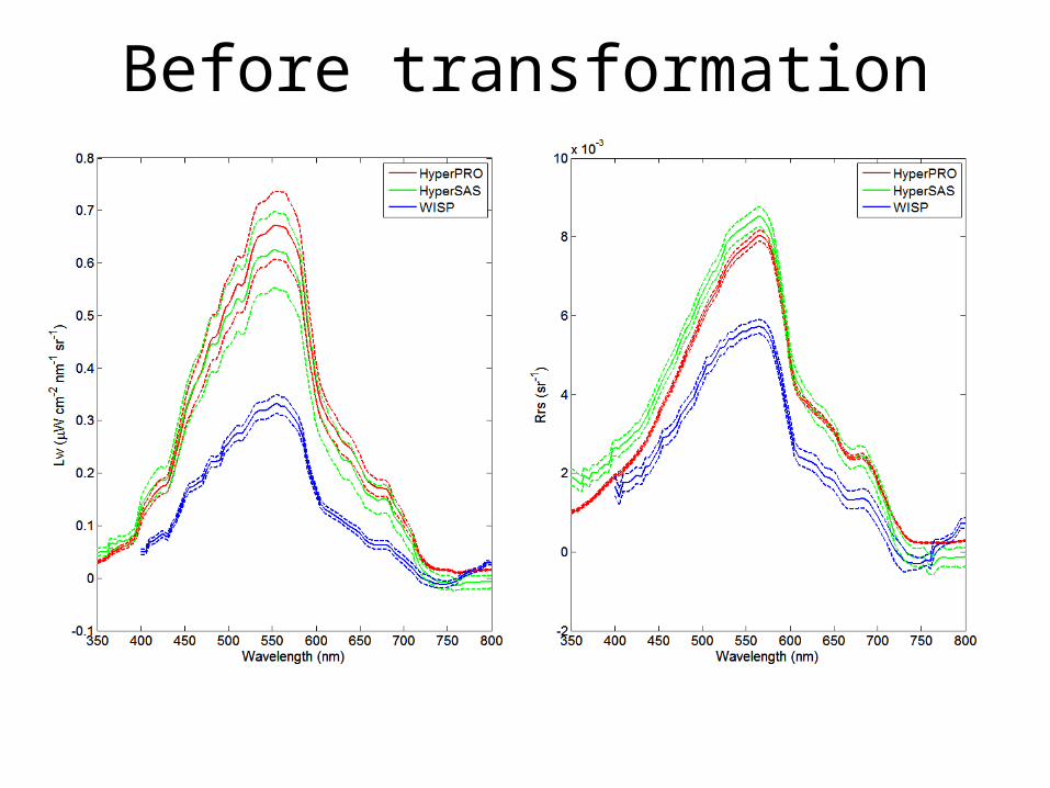
Before transformation

400 450 500 550 600 650 700 750 8000
0.2
0.4
0.6
0.8
1
1.2
1.4Lw Comparison with Transform
Wavelength (nm)
Lw (
uW/c
m2/n
m/s
r)
HyperPro TransformedStdErrWISP TransformedStdErrHyperSASStdErr
After transformation

400 450 500 550 600 650 700 750 8000
0.005
0.01
0.015Rrs Comparison with Transform
Wavelength (nm)
Rrs
(1/
sr)
HyperPro TransformedStdErrWISP TransformedStdErrHyperSASStdErr
After transformation

Three Lw’s can match if we use ρsky=0.021 instead of 0.028. Therefore, this means we overcorrected sky radiance initially (?).
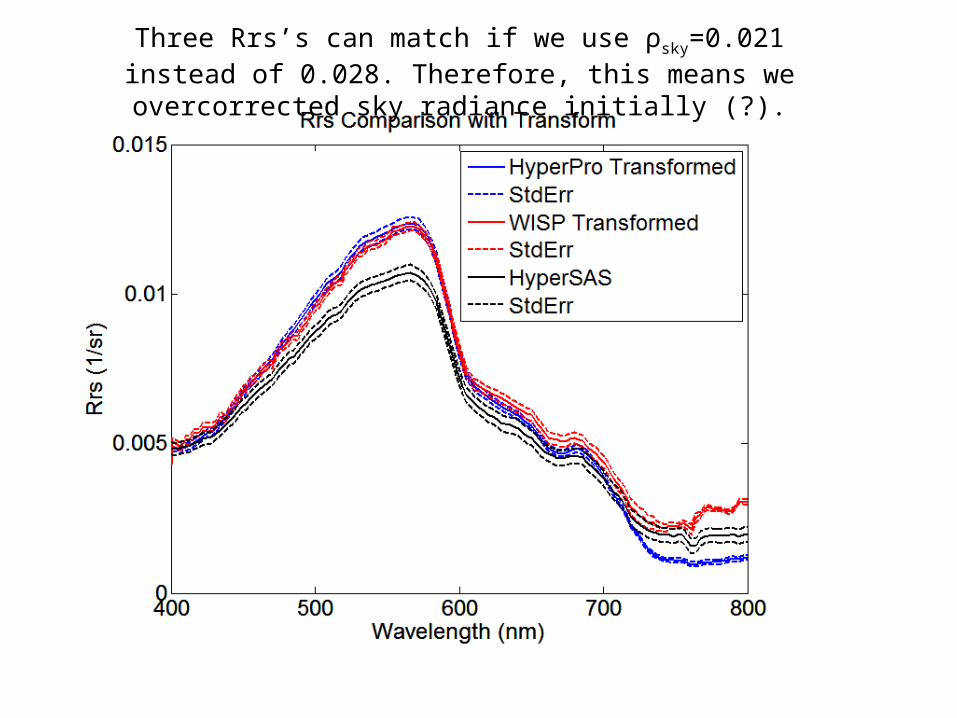
Three Rrs’s can match if we use ρsky=0.021 instead of 0.028. Therefore, this means we overcorrected sky radiance initially (?).

Cruise 1: Ocean Station
400 450 500 550 600 650 700 750 80020
30
40
50
60
70
80
90
100
110Ed Comparison with Transform
Wavelength (nm)
Ed
(uW
/cm
2/n
m)
HyperPro TransformedStdErrWISP TransformedStdErrHyperSASStdErr

400 500 600 700 8000
0.2
0.4
0.6
0.8
1Surface Radiance Comparison with Transform
Wavelength (nm)
Lt (
uW/c
m2/n
m/s
r)
WISP TransformedStdErrHyperSASStdErr

400 500 600 700 8000
5
10
15
20
25Sky Radiance Comparison with Transform
Wavelength (nm)
Lsky
(uW
/cm
2/n
m/s
r)
WISP TransformedStdErrHyperSASStdErr

400 450 500 550 600 650 700 750 800-0.2
-0.1
0
0.1
0.2
0.3
0.4Lw Comparison with Transform
Wavelength (nm)
Lw (
uW/c
m2/n
m/s
r)
HyperPro TransformedStdErrWISP TransformedStdErrHyperSASStdErr

400 450 500 550 600 650 700 750 800-5
-4
-3
-2
-1
0
1
2
3
4
5x 10
-3 Rrs Comparison with Transform
Wavelength (nm)
Rrs
(1/
sr)
HyperPro TransformedStdErrWISP TransformedStdErrHyperSASStdErr

How do these comparisons suggest?
• All three instruments work better under stable conditions. Especially, the two above-water instruments, HyperSAS and WISP may not ideal for wavy ocean surface.
• Under stable condition, the offsets among instruments seem relatively constant. This may due to different calibration methods using for these instruments.
• Therefore, derived Rrs, that Lw over Ed, is more reliable and comparable, but individual radiance and irradiance by a single instrument may not be trustable without providing sufficient calibration information.

Inversion Application Example• Using algorithm developed by Li et al. (2013, RSE,
Vol. 135, pp. 150–166).• The IOP Inversion
Model for InlandWaters (IIMIW) is specifically developed for turbid lake, estuarine, and coastal waters.
• Validated and works well for 8 sites all over the world.

Chlorophyll (mg/m3)
Date Lab Inversed
Jul 15 ~2.1 2.47
Jul 27 ~2.2 1.88
Here we show the inversion results for dock test on July 15 and July 27. The interesting fact is that inversed results are always better when using WISP-measured Rrs(λ). • This may suggest WISP Rrs is more accurate than the other two instruments.
However, it is not certain until further investigation. Measuring Rrs with more than one instruments, if possible, is still recommended.
Inversion Application Example
Rrs(λ) anw(λ), bbp(λ) Pigments

CLOSURE ANALYSIS

Differences between instruments’ response could be explained by:
• Offsets between sensors,• Spatial variations during deployment,• Not accurate information about atmospheric
conditions and sea level state,• Inappropriate angle corrections,• Handling errors (especially for WISP),• …In
corr
ect v
alue
s of
sea
-sur
face
re
flect
ance
fact
or, ρ
Due to the lack of more information, some of the corrections we can perform are only assumptions and we can’t justify them.
Hydrolight model provides a very useful tool which can be used for this purpose.
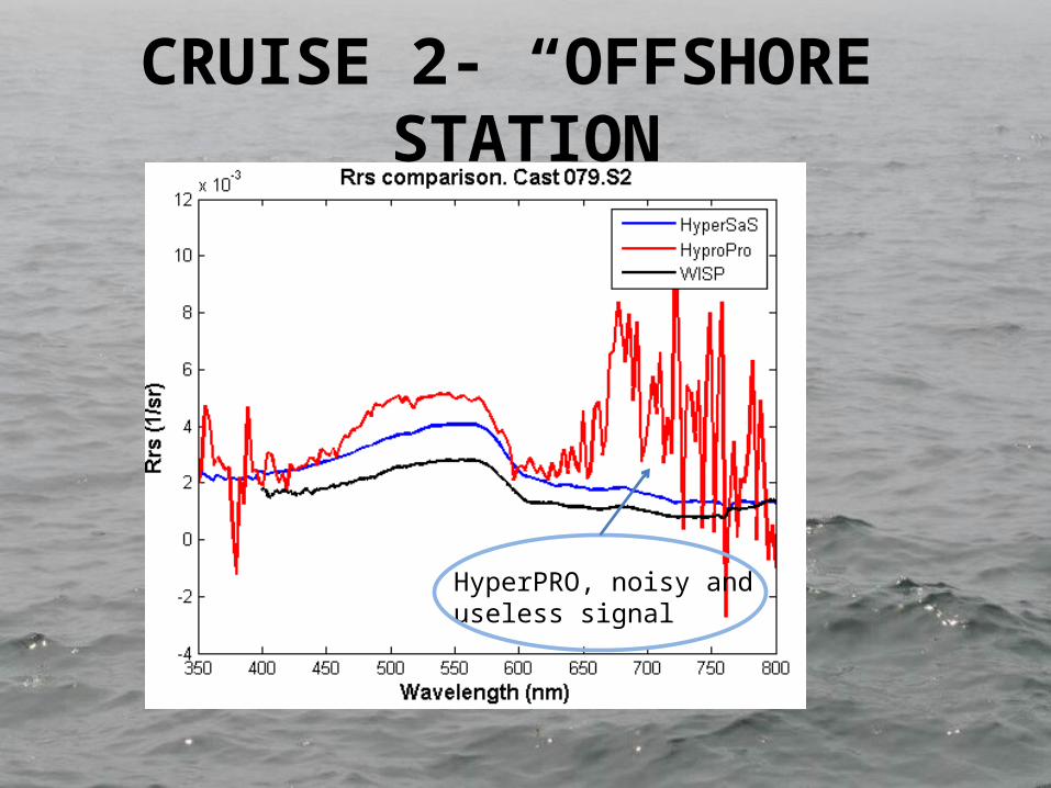
CRUISE 2- “OFFSHORE” STATION
HyperPRO, noisy and useless signal

ECOLIGHT SIMULATIONS:
Simulations under different cloud coverage and wind speeds
Inputs: IOPs (aP,bb,aCDOM)
16%
10%

• Same shape between spectra, different magnitude.1) The measured Rrs at [720-750] significantly higher than zero
open ocean “dark pixel” correction2) Imprecise sky and measurement conditions, unknown try
with another rho values

Mobley (1999)ρ≈0.034 when φ ≈ 135º, θ ≈43º and U=5 m/s
EUCLIDEAN DISTANCE
Without corrections 0.0076
Forcing Rrs[720-750] = 0 8.05E-04
Sea-surface reflectance factor= 0.034
0.0014
.

CRUISE 2- RIVER STATION
• Full overcast (no “dark pixel” corrections nor change of sea-surface reflectance factor).
EUCL. DISTANCE
HyperSAS HyperPRO WISP Ecolight
HyperSAS 0 0.0138 0.0134 0.0215HyperPRO 0.0138 0 0.027 0.008WISP 0.0134 0.027 0 0.0346Ecolight 0.0215 0.008 0.0346 0

• Lab/ Dock test using the Ed sensors under the same light conditions EdPRO= 1.1Ed SAS
Euclidean_dist [Ecolight-HyperPRO]= 0.0036

THANK YOU!

Contact information• If you have questions about the video,
animation, or this PPT, please contact any of us.
Erin Black: [email protected]
Jing Tan: [email protected]
Jing Tao: [email protected]
Linhai Li: [email protected]
Marta Ramrez Perez: [email protected]


