An Introduction to Relativistic QuantumField Theory
Mustafa A. Amin1
Department of Physics & Astronomy, Rice University, Houston, Texas 77005-1827, U.S.A.
Abstract
These are QFT Lecture Notes for Phys 622 at Rice University. At the moment, they constitute a work
in progress, with half of the notes typeset, the other half (later half of chapter 5 onwards) hand-written.
Please report any typos/errors to [email protected].
Last update: 2019/12/12 18:09:38 -06’00’
Preface
These are notes for the Phys 622 course, An Introduction to QFT, at Rice University. This is not a com-
prehensive textbook on QFT. Typically, students from high energy physics and condensed matter theory
take this course at Rice. The condensed matter students go on to take many-body physics as a second
course, whereas the high energy physicists take a more Standard Model focused course next. Along with
high energy physics and condensed matter theory, at times some undergrads, cosmologists/astrophysicists,
biophysicists and theoretical chemists also take this course. This diversity of students, and their academic
paths have guided the preparation of these notes – though it is still focussed on relativistic field theory.
My goal is to set up the foundations of QFT, give a flavor for calculations (with sufficient, simplified
examples) but leave the inevitable complications of the real world to later, more specialized courses.
The course is roughly divided into two parts. In the first part, I only deal with scalar field QFT. It
culminates in the derivation of Feynman rules, and a number of calculations of scattering at tree level.
Spin is only introduced in the second half of the semester, where we focus on how symmetries guide
and constrain the nature of different spin fields. In a one semester course, it was possible to introduce,
but not do any calculations in non-Abelian Gauge theories. I include spontaneous symmetry breaking
in the context of Anderson-Higgs mechanism for particle physics and also its relevance, for example, in
superconductivity here as well. Dictated by student interest, I have also included some brief notes on
solitons and topological considerations in field theories.
At the time of posting, only the first half of the course is typeset in LaTeX, the rest of the notes are
handwritten. Next year, I will hopefully typeset the rest as well.
Acknowledgements
These notes do not contain much in terms of original material. QFT is a mature subject, with many
comprehensive textbooks and pedagogical notes that are easily available. When I taught this course for
the first time (2016), I benefited from Prof. Paul Stevenson’s excellent notes for this class at Rice, which
he taught for many years. His experience showed especially in a wonderfully economical path through the
material. Prof. David Tong’s (Cambridge) notes were the other set of notes I turned to repeatedly.
As far as textbooks go, I learnt QFT from Peskin and Schroeder, as well as by dipping in and out of
A. Zee’s QFT in a Nutshell for inspiration and anecdotes. In preparing these notes, I referred to them
repeatedly. In addition, I thoroughly enjoyed QFT for the Gifted Amateur by Tom Lancaster and Stephen
Blundell. The short chapters in both Zee and Lancaster & Blundell, the appropriately simplified sample
calculations, the pedagogical (and at times whimsical) prose and diagrams made them a pleasure to read.
Both books were also helpful in helping me learn (at a cursory level) condensed matter applications of
QFT from their self-contained chapters.
1
CONTENTS
1 An Invitation 5
1.1 Some Highlights from QFT . . . . . . . . . . . . . . . . . . . . . . . . . . . . . . . . . . . . 5
1.2 Units . . . . . . . . . . . . . . . . . . . . . . . . . . . . . . . . . . . . . . . . . . . . . . . . 6
2 Rapid Review 8
2.1 Special Relativity . . . . . . . . . . . . . . . . . . . . . . . . . . . . . . . . . . . . . . . . . . 8
2.2 Classical Mechanics . . . . . . . . . . . . . . . . . . . . . . . . . . . . . . . . . . . . . . . . . 10
2.2.1 Lagrangian Mechanics . . . . . . . . . . . . . . . . . . . . . . . . . . . . . . . . . . . 10
2.2.2 Hamiltonian Mechanics . . . . . . . . . . . . . . . . . . . . . . . . . . . . . . . . . . 11
2.2.3 Poisson Brackets . . . . . . . . . . . . . . . . . . . . . . . . . . . . . . . . . . . . . . 11
2.3 Quantum Mechanics . . . . . . . . . . . . . . . . . . . . . . . . . . . . . . . . . . . . . . . . 12
2.3.1 Canonical Quantization . . . . . . . . . . . . . . . . . . . . . . . . . . . . . . . . . . 12
2.3.2 Worked Example: Harmonic Oscillators . . . . . . . . . . . . . . . . . . . . . . . . . 13
Canonical Quantization . . . . . . . . . . . . . . . . . . . . . . . . . . . . . . . . . . 14
Creation and Annihilation Operators . . . . . . . . . . . . . . . . . . . . . . . . . . . 14
2.4 Special Relativity and Single-Particle Quantum Mechanics . . . . . . . . . . . . . . . . . . . 16
3 Quantizing Scalar Fields 17
3.1 Classical Scalar Fields . . . . . . . . . . . . . . . . . . . . . . . . . . . . . . . . . . . . . . . 17
3.1.1 Poisson Brackets . . . . . . . . . . . . . . . . . . . . . . . . . . . . . . . . . . . . . . 18
3.2 Canonical Quantization of Scalar Fields . . . . . . . . . . . . . . . . . . . . . . . . . . . . . 19
3.2.1 Free Quantum Scalar Field . . . . . . . . . . . . . . . . . . . . . . . . . . . . . . . . 19
3.2.2 Propagation Amplitudes and Positive and Negative Frequency Solutions . . . . . . . 24
3.2.3 Green’s functions . . . . . . . . . . . . . . . . . . . . . . . . . . . . . . . . . . . . . . 25
3.2.4 Causality . . . . . . . . . . . . . . . . . . . . . . . . . . . . . . . . . . . . . . . . . . 25
3.2.5 Free Complex Scalar Fields . . . . . . . . . . . . . . . . . . . . . . . . . . . . . . . . 26
Canonical Quantization . . . . . . . . . . . . . . . . . . . . . . . . . . . . . . . . . . 26
Mode expansion . . . . . . . . . . . . . . . . . . . . . . . . . . . . . . . . . . . . . . 27
Charge . . . . . . . . . . . . . . . . . . . . . . . . . . . . . . . . . . . . . . . . . . . 27
Causality, again . . . . . . . . . . . . . . . . . . . . . . . . . . . . . . . . . . . . . . . 29
Non-relativistic Fields . . . . . . . . . . . . . . . . . . . . . . . . . . . . . . . . . . . 29
2
4 Weakly Interacting Fields 30
4.1 Adding Interactions . . . . . . . . . . . . . . . . . . . . . . . . . . . . . . . . . . . . . . . . 30
4.1.1 Perturbative Control . . . . . . . . . . . . . . . . . . . . . . . . . . . . . . . . . . . . 31
4.2 Time Evolution in the Interaction Picture . . . . . . . . . . . . . . . . . . . . . . . . . . . . 32
4.2.1 The S-matrix . . . . . . . . . . . . . . . . . . . . . . . . . . . . . . . . . . . . . . . . 34
Why use the Interaction Picture? . . . . . . . . . . . . . . . . . . . . . . . . . . . . . 35
Green’s Functions . . . . . . . . . . . . . . . . . . . . . . . . . . . . . . . . . . . . . 35
LSZ Reduction Formula . . . . . . . . . . . . . . . . . . . . . . . . . . . . . . . . . . 35
Gell-Mann-Low Theorem . . . . . . . . . . . . . . . . . . . . . . . . . . . . . . . . . 36
4.2.2 Normal Ordering and Wick’s theorem . . . . . . . . . . . . . . . . . . . . . . . . . . 36
Normal Ordering . . . . . . . . . . . . . . . . . . . . . . . . . . . . . . . . . . . . . . 36
Contractions and Wick’s Theorems . . . . . . . . . . . . . . . . . . . . . . . . . . . . 37
Wick’s Theorem for Ordinary Products . . . . . . . . . . . . . . . . . . . . . . . . . 38
Wick’s Theorem for Time-Ordered Products . . . . . . . . . . . . . . . . . . . . . . 39
4.2.3 Feynman Propagator . . . . . . . . . . . . . . . . . . . . . . . . . . . . . . . . . . . . 39
Feynman Propagator in Momentum Space . . . . . . . . . . . . . . . . . . . . . . . . 40
4.3 Perturbative Calculations in A Toy Model . . . . . . . . . . . . . . . . . . . . . . . . . . . . 41
4.3.1 Decay: “γ”→ e− + e+ . . . . . . . . . . . . . . . . . . . . . . . . . . . . . . . . . . . 41
Initial and Final States . . . . . . . . . . . . . . . . . . . . . . . . . . . . . . . . . . 42
Dyson Expansion . . . . . . . . . . . . . . . . . . . . . . . . . . . . . . . . . . . . . . 42
Contractions . . . . . . . . . . . . . . . . . . . . . . . . . . . . . . . . . . . . . . . . 43
The Matrix Elements . . . . . . . . . . . . . . . . . . . . . . . . . . . . . . . . . . . 43
4.3.2 Scattering: e− + e− → e− + e− . . . . . . . . . . . . . . . . . . . . . . . . . . . . . . 44
Initial and Final States . . . . . . . . . . . . . . . . . . . . . . . . . . . . . . . . . . 44
Dyson Expansion . . . . . . . . . . . . . . . . . . . . . . . . . . . . . . . . . . . . . . 44
Contractions . . . . . . . . . . . . . . . . . . . . . . . . . . . . . . . . . . . . . . . . 44
Matrix Element . . . . . . . . . . . . . . . . . . . . . . . . . . . . . . . . . . . . . . . 45
Feynman Rules in x-space . . . . . . . . . . . . . . . . . . . . . . . . . . . . . . . . . 45
Feynman Rules in k-space . . . . . . . . . . . . . . . . . . . . . . . . . . . . . . . . . 46
4.3.3 Scattering: e+ + e− → e+ + e− . . . . . . . . . . . . . . . . . . . . . . . . . . . . . . 48
Initial and Final States . . . . . . . . . . . . . . . . . . . . . . . . . . . . . . . . . . 48
Dyson Expansion . . . . . . . . . . . . . . . . . . . . . . . . . . . . . . . . . . . . . . 48
Contractions . . . . . . . . . . . . . . . . . . . . . . . . . . . . . . . . . . . . . . . . 48
Matrix Element and Feynman Diagrams . . . . . . . . . . . . . . . . . . . . . . . . . 49
4.3.4 The Diagrammar’s way . . . . . . . . . . . . . . . . . . . . . . . . . . . . . . . . . . 50
4.3.5 Amplitudes to Observables . . . . . . . . . . . . . . . . . . . . . . . . . . . . . . . . 51
Decay rate . . . . . . . . . . . . . . . . . . . . . . . . . . . . . . . . . . . . . . . . . 52
Differential cross-section . . . . . . . . . . . . . . . . . . . . . . . . . . . . . . . . . . 52
Amplitudes and cross-sections to forces . . . . . . . . . . . . . . . . . . . . . . . . . 53
4.3.6 Beyond Leading Order . . . . . . . . . . . . . . . . . . . . . . . . . . . . . . . . . . . 54
Connected and Amputated Contributions . . . . . . . . . . . . . . . . . . . . . . . . 54
Divergences at higher orders . . . . . . . . . . . . . . . . . . . . . . . . . . . . . . . 55
4.3.7 A Taste of Renormalization . . . . . . . . . . . . . . . . . . . . . . . . . . . . . . . . 56
Flow of Physical Coupling Constants . . . . . . . . . . . . . . . . . . . . . . . . . . . 59
4.4 Summary . . . . . . . . . . . . . . . . . . . . . . . . . . . . . . . . . . . . . . . . . . . . . . 60
3
5 Symmetry and Fields 61
5.1 Spacetime and Internal Symmetries . . . . . . . . . . . . . . . . . . . . . . . . . . . . . . . . 61
5.1.1 Noether’s Theorem and its Consequences . . . . . . . . . . . . . . . . . . . . . . . . 61
5.1.2 Internal Symmetries . . . . . . . . . . . . . . . . . . . . . . . . . . . . . . . . . . . . 63
5.1.3 Spacetime Symmetries . . . . . . . . . . . . . . . . . . . . . . . . . . . . . . . . . . . 64
Translations . . . . . . . . . . . . . . . . . . . . . . . . . . . . . . . . . . . . . . . . . 64
Boosts and Rotations . . . . . . . . . . . . . . . . . . . . . . . . . . . . . . . . . . . 65
Finite Transformations . . . . . . . . . . . . . . . . . . . . . . . . . . . . . . . . . . . 68
5.2 Lorentz Transformations of Fields . . . . . . . . . . . . . . . . . . . . . . . . . . . . . . . . . 68
5.3 Spin 1 . . . . . . . . . . . . . . . . . . . . . . . . . . . . . . . . . . . . . . . . . . . . . . . . 70
5.3.1 Massive Vector Fields . . . . . . . . . . . . . . . . . . . . . . . . . . . . . . . . . . . 70
Equations of Motion . . . . . . . . . . . . . . . . . . . . . . . . . . . . . . . . . . . . 71
Plane-Wave Solutions & Mode Expansion . . . . . . . . . . . . . . . . . . . . . . . . 71
Canonical Quantization . . . . . . . . . . . . . . . . . . . . . . . . . . . . . . . . . . 72
Propagator . . . . . . . . . . . . . . . . . . . . . . . . . . . . . . . . . . . . . . . . . 72
5.3.2 Massless Vector Fields . . . . . . . . . . . . . . . . . . . . . . . . . . . . . . . . . . . 73
Gauge Freedom . . . . . . . . . . . . . . . . . . . . . . . . . . . . . . . . . . . . . . . 73
Connecting to the “usual” Maxwell’s Equations . . . . . . . . . . . . . . . . . . . . . 73
Solutions in Coulumb Gauge . . . . . . . . . . . . . . . . . . . . . . . . . . . . . . . 74
Canonical Quantization in Coulumb Gauge . . . . . . . . . . . . . . . . . . . . . . . 74
5.4 Spin 1/2 . . . . . . . . . . . . . . . . . . . . . . . . . . . . . . . . . . . . . . . . . . . . . . . 75
5.4.1 Dirac Spinors . . . . . . . . . . . . . . . . . . . . . . . . . . . . . . . . . . . . . . . . 75
The Dirac Equation and its Solutions . . . . . . . . . . . . . . . . . . . . . . . . . . 76
Equation of Motion . . . . . . . . . . . . . . . . . . . . . . . . . . . . . . . . . . . . 76
Mode Expansion . . . . . . . . . . . . . . . . . . . . . . . . . . . . . . . . . . . . . . 77
Quantization . . . . . . . . . . . . . . . . . . . . . . . . . . . . . . . . . . . . . . . . 78
5.5 Quantum Electrodynamics . . . . . . . . . . . . . . . . . . . . . . . . . . . . . . . . . . . . . 79
5.5.1 Local Gauge Invariance . . . . . . . . . . . . . . . . . . . . . . . . . . . . . . . . . . 81
Global Symmetries . . . . . . . . . . . . . . . . . . . . . . . . . . . . . . . . . . . . . 81
Local Symmetries . . . . . . . . . . . . . . . . . . . . . . . . . . . . . . . . . . . . . 81
5.5.2 Yang-Mills Theories . . . . . . . . . . . . . . . . . . . . . . . . . . . . . . . . . . . . 82
5.6 Broken Symmetries . . . . . . . . . . . . . . . . . . . . . . . . . . . . . . . . . . . . . . . . . 83
5.6.1 Preliminaries – Nambu-Goldstone Theorem . . . . . . . . . . . . . . . . . . . . . . . 83
5.6.2 Anderson-Higgs Mechanism and Applications . . . . . . . . . . . . . . . . . . . . . . 83
5.6.3 Defects . . . . . . . . . . . . . . . . . . . . . . . . . . . . . . . . . . . . . . . . . . . 83
Topological Solitons . . . . . . . . . . . . . . . . . . . . . . . . . . . . . . . . . . . . 83
5.7 QFT in Nontrivial Classical Backgrounds . . . . . . . . . . . . . . . . . . . . . . . . . . . . 83
A Mathematical Preliminaries 84
A.1 Fourier Transforms . . . . . . . . . . . . . . . . . . . . . . . . . . . . . . . . . . . . . . . . . 84
A.2 Delta Functions . . . . . . . . . . . . . . . . . . . . . . . . . . . . . . . . . . . . . . . . . . . 85
A.3 Functionals . . . . . . . . . . . . . . . . . . . . . . . . . . . . . . . . . . . . . . . . . . . . . 86
A.4 Green’s Functions . . . . . . . . . . . . . . . . . . . . . . . . . . . . . . . . . . . . . . . . . 87
A.5 Contour Integration . . . . . . . . . . . . . . . . . . . . . . . . . . . . . . . . . . . . . . . . 87
A.6 Groups and Representation Theory . . . . . . . . . . . . . . . . . . . . . . . . . . . . . . . . 88
References . . . . . . . . . . . . . . . . . . . . . . . . . . . . . . . . . . . . . . . . . . . . . . . . . 88
4
CHAPTER 1
AN INVITATION
In “Classical” Mechanics, particles are objects localized in space. Their position varies with time ac-
cording to ordinary differential equations. In single particle quantum mechanics, position became an
operator and the notion of a particle became “fuzzier” (think about localized probability density in terms
of wavefunctions, uncertainty principle etc.)
Classical fields on the other hand are extended objects, with values at each point in space. Typically,
partial differential equations govern the time evolution of fields (think of the electromagnetic fields: E(t,x)
and B(t,x) governed by Maxwell’s equations). How can we think about quantum mechanics of fields ?
What is the a connection between fields and particles?
In this course, we will take the view point of the field and particles being part of the same physical
entity. For example, photons are quantized excitations of the electromagnetic field. Equivalently we can
think of the electromagnetic field as a collection of quantized excitations: photons. Similar statements
hold for the electron and the electron field, quarks and a quark field ... you get the idea.
What is this course about?
This course is about learning the rules that govern the behavior of fields and their excitations (parti-
cles), insisting on consistency with Quantum Mechanics and Special Relativity. Symmetries will play an
important role in determining these rules.1
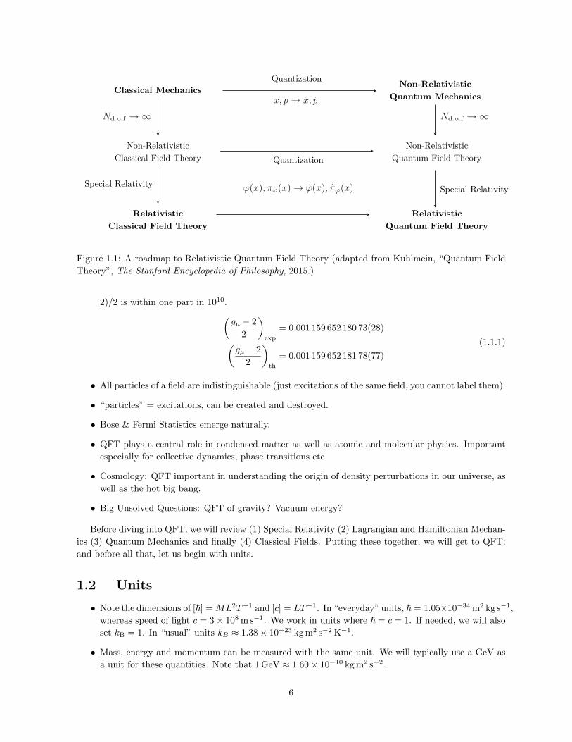
For a heuristic conceptual roadmap to QFT, see Fig. 1.1. An important aspect of QFT in general is
that we are forced to deal with an infinite number of degrees of freedom. This, as we will see, this will
end up being connected to merging of special relativity and quantum mechanics. These infinite degrees of
freedom will also lead to some glaring difficulties in calculating observables; these difficulties will require
conceptual leaps to overcome them. As always, these rough and somewhat abstract statements will make
more sense when we have done some concrete examples. I hope that the course will allow you to appreciate
(and perhaps even make you uneasy) about some of the heuristic statements made in this introduction.
1.1 Some Highlights from QFT
• QFT is one of the most successful theoretical frameworks we have. In Quantum Electrodynamics
(QED), agreement between theory and experiment for the anamolous muon magnetic moment (gµ−1 Occasionally we will work in the non-relativistic limit, and sometimes only talk about classical fields also. The tools
developed here will remain useful.
5
x, p ! x, p
'(x),'(x) ! '(x), '(x)
Nd.o.f ! 1
Classical Mechanics Non-Relativistic Quantum Mechanics
Relativistic Classical Field Theory
Relativistic Quantum Field Theory
Non-Relativistic Classical Field Theory
Non-Relativistic Quantum Field Theory
Nd.o.f ! 1
Special Relativity Special Relativity
Quantization
Quantization
Figure 1.1: A roadmap to Relativistic Quantum Field Theory (adapted from Kuhlmein, “Quantum Field
Theory”, The Stanford Encyclopedia of Philosophy, 2015.)
2)/2 is within one part in 1010.
(gµ − 2
2
)
exp
= 0.001 159 652 180 73(28)
(gµ − 2
2
)
th
= 0.001 159 652 181 78(77)
(1.1.1)
• All particles of a field are indistinguishable (just excitations of the same field, you cannot label them).
• “particles” = excitations, can be created and destroyed.
• Bose & Fermi Statistics emerge naturally.
• QFT plays a central role in condensed matter as well as atomic and molecular physics. Important
especially for collective dynamics, phase transitions etc.
• Cosmology: QFT important in understanding the origin of density perturbations in our universe, as
well as the hot big bang.
• Big Unsolved Questions: QFT of gravity? Vacuum energy?
Before diving into QFT, we will review (1) Special Relativity (2) Lagrangian and Hamiltonian Mechan-
ics (3) Quantum Mechanics and finally (4) Classical Fields. Putting these together, we will get to QFT;
and before all that, let us begin with units.
1.2 Units
• Note the dimensions of [~] = ML2T−1 and [c] = LT−1. In “everyday” units, ~ = 1.05×10⁻³⁴ m2 kg s−1,
whereas speed of light c = 3× 10⁸ m s−1. We work in units where ~ = c = 1. If needed, we will also
set kB = 1. In “usual” units kB ≈ 1.38× 10⁻²³ kg m2 s−2 K−1.
• Mass, energy and momentum can be measured with the same unit. We will typically use a GeV as
a unit for these quantities. Note that 1 GeV ≈ 1.60× 10⁻¹⁰ kg m2 s−2.
6
• Length and time intervals have the same units. We will typically use GeV−1 as a unit for them.
• examples: mass of proton = 0.938 GeV = 0.938 GeV/c2 ≈ 10−27 kg), size of a proton ∼ 5 GeV−1 =
5GeV−1 ~c ≈ 10−15 m = 1 fermi).
Exercise 1.2.1 : Our universe if filled with blackbody radiation (Cosmic Microwave Background) left over
from the time when the first atoms formed. The present temperature of this radiation is ∼ 3K. Using
dimensional analysis, make an order of magnitude estimate of the number of density of photons in the
CMB in units of (i) GeV3 (ii) cm−3.
Exercise 1.2.2 : (1) If you drop a tomato from a height of ∼ 1 meter, what is its kinetic energy just before
it hits the ground in (i) Joules (ii) GeV? (2) At what height would you have to drop an ant (∼ 2 mg) for
it’s kinetic to be of order a GeV when it hits the ground. (3) What is the typical center of mass energy of
protons at the Large Hadron Collider? (4) What is the ionization energy of a Hydrogen atom ?
7
CHAPTER 2
RAPID REVIEW
In this chapter I review relevant aspects of Einstein’s Special Theory of Relativity, Lagrangian and Hamil-
tonian Mechanics as well as Quantum Mechanics for a countable (and finite) number of degrees of freedom.
Though you are likely familiar with at least some of this material, some formal aspects such as Poisson
Brackets and time-evolution operators introduced here might not have been covered in earlier courses.
For most of this course we will work in natural units with ~ = c = 1 where ~ and c are the Planck’s
constant and speed of light respectively. In this review chapter, I set c = 1 so length and time have the
same units, but do not set ~ = 1 since it helps in seeing quantum aspects more clearly.
2.1 Special Relativity
In two sentences, here is Einstein’s Special Theory of Relativity:
• The laws of physics are the same in all intertial frames.
• The speed of light (in vacuum) c is independent of the reference frame.
Interval and the metric: The inifinitesimal, frame-invariant spacetime interval:
ds2 ≡ gµνdxµdxν with µ, ν = 0, 1, 2, 3 . (2.1.1)
where “0” labels the time co-ordinate. We have adopted the Einstein summation convention, where
repeated upstairs and downstairs indices are summed over. gµν are components of the metric tensor
which (among other responsibilities), determines the interval between events. Think of gµν as entires of
a matrix g, that is g(µ, ν) ≡ gµν , where the first index labels the row, and the second the column with
µ, ν = 0, 1, 2, 3. In cartesian co-ordinates (and with slight abuse of notation):
gµν =
1 0 0 0
0 −1 0 0
0 0 −1 0
0 0 0 −1
, (2.1.2)
Explicity ds2 = (dx0)2 − δijdxidxj = dt2 − dx · dx. If the interval corresponding to nearby events
ds2 < 0(> 0), then the events are said to be connected by a space-like (time-like) interval. ds2 = 0
corresponds to a light-like interval. The same definitions carry over for finite intervals (obtained by joining
together infinitesimal intervals ∼∫ds). One event can influence another only if the interval between them
8
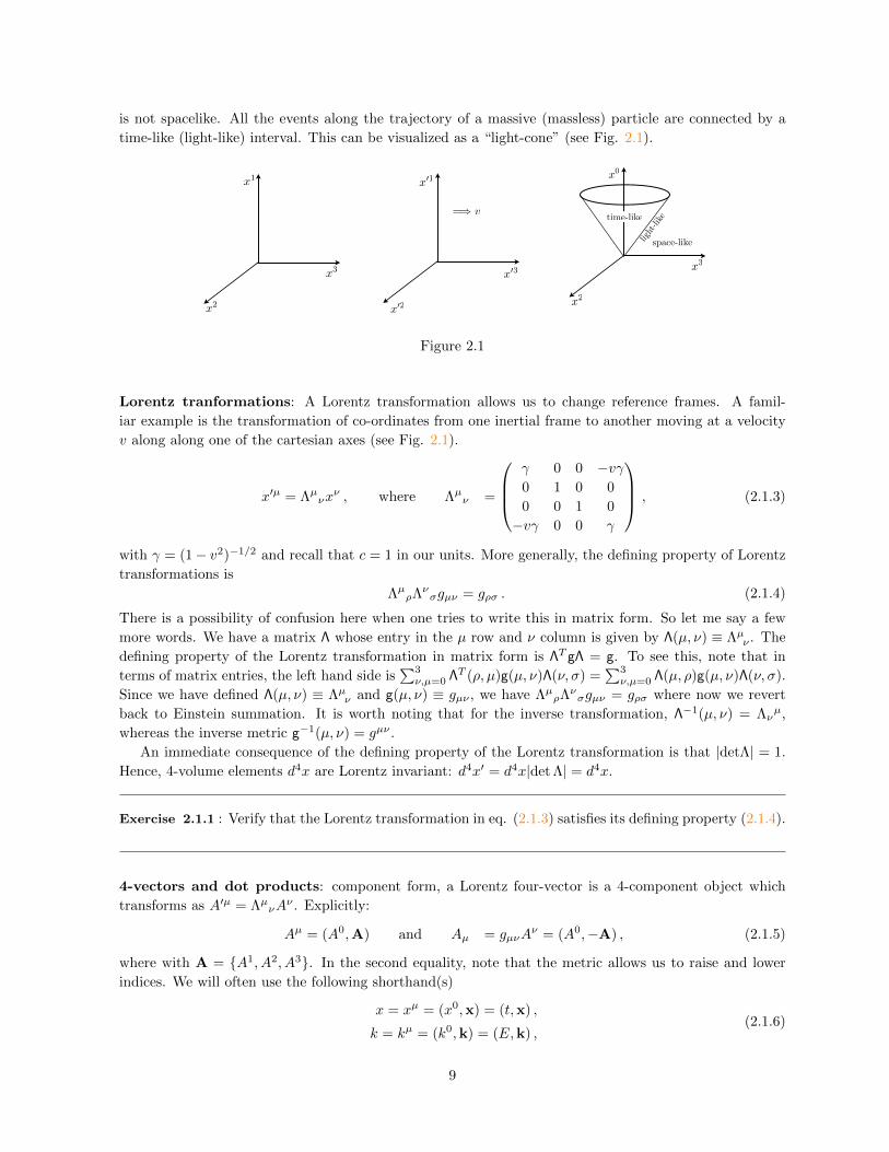
is not spacelike. All the events along the trajectory of a massive (massless) particle are connected by a
time-like (light-like) interval. This can be visualized as a “light-cone” (see Fig. 2.1).
x1
x3
x2
x01
x02
x03
=) v
x3
x2
x0
time-like
space-likelight
-like
Figure 2.1
Lorentz tranformations: A Lorentz transformation allows us to change reference frames. A famil-
iar example is the transformation of co-ordinates from one inertial frame to another moving at a velocity
v along along one of the cartesian axes (see Fig. 2.1).
x′µ = Λµνxν , where Λµν =
γ 0 0 −vγ0 1 0 0
0 0 1 0
−vγ 0 0 γ
, (2.1.3)
with γ = (1− v2)−1/2 and recall that c = 1 in our units. More generally, the defining property of Lorentz
transformations is
ΛµρΛνσgµν = gρσ . (2.1.4)
There is a possibility of confusion here when one tries to write this in matrix form. So let me say a few
more words. We have a matrix Λ whose entry in the µ row and ν column is given by Λ(µ, ν) ≡ Λµν . The
defining property of the Lorentz transformation in matrix form is ΛT gΛ = g. To see this, note that in
terms of matrix entries, the left hand side is∑3ν,µ=0 ΛT (ρ, µ)g(µ, ν)Λ(ν, σ) =
∑3ν,µ=0 Λ(µ, ρ)g(µ, ν)Λ(ν, σ).
Since we have defined Λ(µ, ν) ≡ Λµν and g(µ, ν) ≡ gµν , we have ΛµρΛνσgµν = gρσ where now we revert
back to Einstein summation. It is worth noting that for the inverse transformation, Λ−1(µ, ν) = Λνµ,
whereas the inverse metric g−1(µ, ν) = gµν .
An immediate consequence of the defining property of the Lorentz transformation is that |detΛ| = 1.
Hence, 4-volume elements d4x are Lorentz invariant: d4x′ = d4x|det Λ| = d4x.
Exercise 2.1.1 : Verify that the Lorentz transformation in eq. (2.1.3) satisfies its defining property (2.1.4).
4-vectors and dot products: component form, a Lorentz four-vector is a 4-component object which
transforms as A′µ = ΛµνAν . Explicitly:
Aµ = (A0,A) and Aµ = gµνAν = (A0,−A) , (2.1.5)
where with A = A1, A2, A3. In the second equality, note that the metric allows us to raise and lower
indices. We will often use the following shorthand(s)
x = xµ = (x0,x) = (t,x) ,
k = kµ = (k0,k) = (E,k) ,(2.1.6)
9
where in the last line we are thinking of k as the four-momentum of a particle, with E being the energy.
Their dot product is Lorentz invariant (ie. its value does not change under Lorentz transformations)
x · k = gµνxµkν = xµk
µ = xµkµ = Et− x · k ,kµkµ = E2 − |k|2 = m2 .
(2.1.7)
where m is the rest-mass of the particle.
Some useful differential operators are listed below:
∂µ =∂
∂xµ= (∂0,∇) and ∂µ = (∂0,−∇) ,
= ∂µ∂µ = ∂2
t −∇2 and ∂ ·A = ∂µAµ = ∂0A
0 +∇ ·A .(2.1.8)
Exercise 2.1.2 : Show that f(x) = eik·x satisfies (+m2)f(x) = 0 only if kµkµ = m2.
Exercise 2.1.3 : Consider two reference frames related by the Lorentz transformation in eq. (2.1.3).
Let xµ(P ) =(x0P , 0, 0, x
3P
)and xµ(Q) =
(x0Q, 0, 0, x
3Q
)be the co-ordinates of two events P and Q in
the “unprimed” frame. The co-ordinates of these events in the “primed” frame are given by x′µ(P ) =(x′0P , 0, 0, x
′3P
)and x′µ(Q) =
(x′0Q, 0, 0, x
′3Q
). Show that if the events are not simultaneous (x0
P 6= x0Q), and
are space-like separated in the unprimed frame (i.e. ∆xµ∆xµ < 0 where ∆xµ = xµ(P ) − xµ(Q)), then
there exists a velocity v such that in the primed frame, the events are simultaneous x′0P = x′0Q. Find this
velocity v.
While simultaneity is frame-dependent, intervals are not. That is, ∆x′µ∆x′µ = ∆xµ∆xµ. Hence the
space-like, time-like and light-like nature of intervals is invariant under Lorentz transformations.
2.2 Classical Mechanics
I am going to go through a quick, formal review of classical mechanics with an eye towards Quantum
Mechanics.
2.2.1 Lagrangian Mechanics
Start with a (given) Lagrangian L(qα, qα, t) where qα are the generalized co-ordinate of the system (α =
1, 2 . . . N). The equations of motion for qα are obtained by extremizing the Action:
S =
∫ tf
ti
dtL(qα, qα, t) , (2.2.1)
That is qα(t) are such that for qα(t) → qα(t) + δqα(t) (where δqα(t) are arbitrary apart from δq(ti) =
δq(tf) = 0) we have δS = 0. For δS = 0, qα must satisfy (see Appendix A.3):
d
dt
(∂L
∂qα
)=
∂L
∂qαEuler-Lagrange equations (2.2.2)
10
For example, for a collection of coupled harmonic oscillators with unit mass and time-independent cou-
plings1 Mαρ:
L(qα, qα) =
N∑
α=1
(1
2q2α −
N∑
ρ=1
1
2Mαρ qαqρ
),
d
dt
(∂L
∂qα
)=
∂L
∂qα
=⇒ qα +
N∑
ρ=1
Mαρqρ = 0 .
(2.2.3)
2.2.2 Hamiltonian Mechanics
The Hamiltonian is a Legendre transform of the Lagrangian and contains the same information as the
Lagrangian. In Quantum Mechanics and QFT, the Hamiltonian is often more convenient to work with,
so lets do a quick review:
pα ≡∂L
∂qαconjugate momentum
H ≡N∑
α=1
(pαqα)− L Hamiltonian
qα =∂H
∂pα, pα = − ∂H
∂qαHamilton’s equations
(2.2.4)
For the coupled harmonic oscillators example,
pα = qα ,
H =
N∑
α=1
(1
2p2α +
N∑
ρ=1
1
2Mαρ qαqρ
),
pα = −N∑
ρ=1
Mαρ qρ .
(2.2.5)
2.2.3 Poisson Brackets
The Poisson Bracket is defined as:
f(qα, pα), g(qα, pα) ≡N∑
α=1
(∂f
∂qα
∂g
∂pα− ∂f
∂pα
∂g
∂qα
), (2.2.6)
where f and g are arbitrary functions on the space of generalized co-ordinates and their conjugate momenta.
The time evolution of f(qα, pα, t) is given by
df
dt= f,H+
∂f
∂t. (2.2.7)
which you can see immediately by noting that df/dt =∑α[(∂f/∂qα)qα + (∂f/∂pα)pα] + ∂f/∂t and using
Hamilton’s equations of motion for pα and qα. If the function f does not explicitly depend on time, then
df
dt= f,H . (2.2.8)
1Typically, we consider Mαρ that only couples nearest neighbors.
11
The time evolution of f is generated by H. In particular, for f = qα and g = pρ, we have
qα, pρ = δαρ . (2.2.9)
Similarly, qα, qρ = pα, pρ = 0. The time evolution equations for qα and pρ become
dqαdt
= qα, H , anddpαdt
= pα, H . (2.2.10)
The last two equations are equivalent to Hamilton’s equations of motion, and also to the Euler-Lagrange
equations.
Exercise 2.2.1 : For the coupled harmonic oscillator example in eq. (2.2.5), evaluate the Poisson Brackets
pα, H, to recover pα = −∑ρMαρqρ.
2.3 Quantum Mechanics
I am going to review relevant aspects of Quantum Mechanics; the results here are the most relevant part
of this review chapter.
2.3.1 Canonical Quantization
One route to getting from classical to quantum mechanics is as follows (thanks to Dirac2):
• replace the co-ordinates and momenta by operators (think of them as matrices)
qα, pα −→ qα, pα . (2.3.1)
The functions f and g inherit the operator structure from p and q: f, g → f , g.
• Replace the Poisson Bracket by the “Commutator”
f, g → − i~
[f , g]. (2.3.2)
Note the appearance of i and Planck’s constant ~.The commutator is defined as[f , g]≡ f g − gf . (2.3.3)
Operators f and g do not necessarily commute. For f = qα and q = pρ, we get
[qα, pρ] = i~δαρ . (2.3.4)
This should look familiar! Also note that [qα, qρ] = [pα, qρ] = 0. One could directly start from these
commutation relations as well, without going through Poisson Brackets.
• The time evolution of f(qα, pα) (no explicit time dependence) is given by
df
dt= − i
~
[f , H
]. (2.3.5)
For co-ordinates and momenta,
dqαdt
= − i~
[qα, H
], and
dpαdt
= − i~
[pα, H
]. (2.3.6)
2Dirac, Principles of Quantum Mechanics, Oxford University Press (1982)
12
Comments:
• This above quantization procedure procedure is not a guarantee of finding the correct quantum
theory. Higher order terms in ~ might be relevant. The above procedure is motivated by recovering
classical physics in the limit “~ → 0”. There also exists an ambiguity in the above procedure
regarding the orderings of operators; which one is correct? q3p2 → q3p2 or q3p2 → p2q3? Ultimately,
you have to check with nature whether you have the correct quantum Hamiltonian.
• Heisenberg Picture : Note that we are working in the “Heisenberg Picture” where the operators
f(qα, pα) evolve with time according to3
df
dt= − i
~
[f , H
], or equivalently f(t) = e
i~ H(t−t0)f(t0)e−
i~ H(t−t0) . (2.3.7)
The states |ψ〉 of the system is time-independent. To find the expectation value of an observable
corresponding to the operator f(t) in a given state |ψ〉, we have to calculate 〈ψ|f(t)|ψ〉. Notice that
it is a combination of operators sandwiched between states that appears in the expectation values.
• Schrodinger Picture: A mathematically equivalent way of thinking about time evolution of quan-
tum systems is to think of states |ψ(t)〉s evolving with time, and the operators fs being time-
independent. States evolve according to the Schrodinger equation4:
d
dt|ψ(t)〉s = − i
~H|ψ(t)〉s , or equivalently |ψ(t)〉s = e−
i~ H(t−t0)|ψ(t0)〉s . (2.3.8)
As you can check, by setting |ψ(t0)〉s = |ψ〉 and f(t0) = fs, the expectation values constructed in
either picture will yield the same answer s〈ψ(t)|fs|ψ(t)〉s = 〈ψ|f(t)|ψ〉. The same argument works for
arbitrary matrix elements: fab = s〈a(t)|fs|b(t)〉s = 〈a|f(t)|b〉 (think about transition probabilities),
thus observables will be equal when calculated in either picture.
Exercise 2.3.1 : Verify that f(t) = ei~ H(t−t0)f(t0)e−
i~ H(t−t0) is a solution of df/dt = −(i/~)[f , H]. Be
careful about the fact that H is an operator, not a number. You should interpret eA =∑∞n=0(1/n!)An.
2.3.2 Worked Example: Harmonic Oscillators
The career of a young theoretical physicist consists of treating the harmonic oscillator in ever-increasing
levels of abstraction – Sidney Coleman
Let us revert once more to coupled harmonic oscillators with unit mass; see equations (2.2.3) and (2.2.5).
For time-independent couplings Mαρ there exists Cαρ such that if qα =∑ρ Cαρqρ, then
H =
N∑
α=1
(1
2p2α +
1
2ω2α q
2α
). (2.3.9)
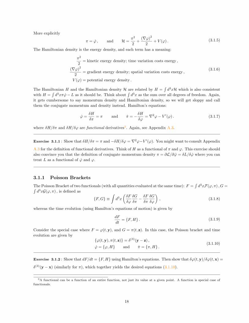
The “tilde” co-ordinates are the normal-modes of the system. For example, for a collection of 2-masses
and three springs (see Fig. 2.2), the two normal modes would be the modes where the masses oscillate
together (in phase) or with an opposite phase. Normal modes are exceptionally convenient, because they
3We assume that H has no explicit time-dependence for simplicity.4The familiar wave-function in position space corresponding to the state |a(t)〉s is obtained via Ψa(t,x) = s〈x|a(t)〉s.
13
q1 q2
q2
q1
Figure 2.2: Normal modes for two masses connected by springs.
evolve independently from each other! For our system (dropping the “tilde” now), we have Hamilton’s
equations
qα = pα , and pα = −ω2αqα . (2.3.10)
Equivalently, the Euler-Lagrange equations are:
qα + ω2αqα = 0 , (2.3.11)
with the solutions qα ∝ e±iωαt.
Canonical Quantization
Let us turn the crank of quantizing our theory. For the system at hand qα, pα −→ qα, pα with [qα, pρ] =
i~δαρ. The Hamiltonian and equations of motion are
H =
N∑
α=1
(1
2p2α +
1
2ω2α q
2α
),
dqαdt
= pα , anddpαdt
= −ω2αqα . (2.3.12)
Exercise 2.3.2 : For the above Hamiltonian, evaluate the commutator [pα, H] using the commutators for
qα and pρ. Then use the time evolution equation (d/dt)pα = −(i/~)[pα, H] to recover (d/dt)pα = −ω2αqα.
It is often useful to remember the following identity for commutators: [ab, c] = a[b, c] + [a, c]b.
Next, we introduce the formalism of creation and annihilation operators, which will turn out to be quite
useful when we deal with fields in the next chapter.
Creation and Annihilation Operators
It is convenient to define the “creation” and “annihilation” operators
aα(t) =
√ωα2~
(qα(t) + i
pα(t)
ωα
)and a†α(t) =
√ωα2~
(qα(t)− i pα(t)
ωα
). (2.3.13)
Recall that qα and pα are Hermitian because they correspond to observables (i.e. they must have real
eigenvalues). These can be inverted to yield
qα(t) =
√~
2ωα
(aα(t) + a†α(t)
)and pα(t) = −i
√~ωα
2
(aα(t)− a†α(t)
). (2.3.14)
14
The time dependence of aα(t) and a†α(t) can be obtained by using our knowledge of dqα/dt and dpα/dt,
which yields (d/dt)aα(t) = −iωαaα(t) and (d/dt)a†α(t) = iωαa†α(t). The solutions are
aα(t) = aα(0)e−iωαt and a†α(t) = a†α(0)e+iωαt . (2.3.15)
Exercise 2.3.3 : Derive (d/dt)aα(t) = −iωαaα(t) and (d/dt)a†α(t) = iωαa†α(t).
Using eq. (2.3.14), we have the “mode-expansion” of qα:
qα(t) =
√~
2ωα
(aα(0)e−iωαt + a†α(0)eiωαt
). (2.3.16)
To reduce clutter, We drop the (0) part in the time-independent creation and annihilation operators, and
simply write
qα(t) =
√~
2ωα
(aαe−iωαt + a†αe
iωαt). (2.3.17)
From now on, when we refer to aα and a†α, we will always mean the time-independent ones. The corre-
sponding expression for pα is
pα(t) = −i√
~ωα2
(aαe−iωαt − a†αeiωαt
). (2.3.18)
Why are aα and a†α useful? It is worth reminding ourselves of the important properties of aα and a†α:
[aα, a
†ρ
]= δαρ ,
[aα, aρ] =[a†α, a
†ρ
]= 0 ,
H =∑
α
(a†αaα +
1
2
)~ωα .
(2.3.19)
Exercise 2.3.4 : Derive the above expressions using the commutators for the co-ordinates and momenta,
the Hamiltonian in eq. (2.3.12) as well as the mode expansions above.
Why the name “creation” and “annihilation” operators? Note another property (that you should verify):[H, aα
]= −~ωαaα , and
[H, a†α
]= ~ωαa†α . (2.3.20)
The last line tells us about creation and annihilation of quanta. To see this, note that if |ψ〉 is an eigenstate
of the H with energy E, then a†α|ψ〉 has an energy E + ~ωα:
Ha†α|ψ〉 = (E + ~ωα)a†α|ψ〉 . (2.3.21)
That is, a†α raises the energy by ~ωα; it “creates” a quantum ~ωα. Similarly,
Haα|ψ〉 = (E − ~ωα)aα|ψ〉 . (2.3.22)
That is, aα lowers the energy by ~ωα; it “annihilates” a quantum ~ωα. The vacuum state is defined as the
state that is annihilated by any aα:
|0〉 ≡ |0, 0 . . . 0〉, where aα|0〉 = 0 . (2.3.23)
15
Each “slot” in |0, 0 . . . 0〉 corresponds to different α = 1, . . . N . We can build normalized eigenstates of
energy by repeatedly acting on the vacuum state using our creation operators
|n1, n2 . . . nN 〉 =
N∏
α=1
(a†α)nα
√nα!|0〉 , (2.3.24)
where nα are the number of quanta (occupation number) with energy ~ωα is this state. Note that
a†αaα|n1, n2 . . . nN 〉 = nα|n1, n2 . . . nN 〉. The total energy of this state
Etot =
N∑
α=1
Eα =
N∑
α=1
(nα +
1
2
)~ωα . (2.3.25)
Even if there are no quanta nα = 0 for all α, we still have vacuum energy Evac =∑Nα=1(1/2)~ωα. This is
important when absolute values of energy matter (e.g. when gravity is involved (“Cosmological Constant”
problem)) or when dealing with non-trivial boundary conditions (“Casimir effect”). In this course we can
ignore this vacuum contribution; for us only differences in energy matter.
Exercise 2.3.5 : Evaluate 〈0|(aα + a†α)4|0〉 using the commutation relations for aα and a†α as well as their
action on the vacuum.
2.4 Special Relativity and Single-Particle Quantum Mechanics
For simplicity of expressions, let ~ = c = 1. Consider a relativistic particle with a Hamiltonian such
that H|k〉 =√
k2 +m2|k〉 for a particle with mass m in its momentum eigenstate. Let us calculate the
“amplitude” A (where the probability ∝ |A|2) of a localized particle moving from (t0 = 0,x0) to (t,x).
That is, we take a localized state |x0〉, time evolve it: e−iH(t−t0)|x0〉, and ask whether this state has an
overlap with 〈x|. To be consistent with special relativity, we must get A = 0 if (t0,x0) and (t,x) are
space-like separated. Upon an explicit calculation5
A = 〈x|e−iH(t−t0)|x0〉 ∼ e−m|x−x0| 6= 0 (2.4.1)
where we have assumed that |x−x0|2 (t− t0)2. This is small, but non-zero. Thus single-particle Quan-
tum Mechanics is inconsistent with Special Relativity. As we will soon see next, a radical new approach
is needed where particle number is not conserved. In anticipation of what is to follow in the next chapter,
and to avoid clutter in this subsection, I have set ~ = 1 and will continue to do so from now onwards.
Comment: QM can be consistent with SR. We have only shown that single-particle QM is inconsistent
with SR. Note that in QFT, the Schrodinger equation: i(d/dt)|ψ〉s = H|ψ〉s is still valid. You have to make
sure you use the correct Hamiltonian made out of operator valued fields, whose evolution is consistent with
SR, and also use appropriate states. Using the Schrodinger equation proves to be rather unwieldy when
dealing with fields, so the formalism (while mathematically equivalent), will look quite different from the
Schrodinger equation.
5see for example, section 8.3 in Lancaster and Blundell, or section 2.1 in Peskin and Schroeder.
16
CHAPTER 3
QUANTIZING SCALAR FIELDS
We are now ready to talk about fields. In this chapter we will limit ourselves to scalar fields. We start with
classical, relativistic scalar fields and then quantize them. Most of this chapter is devoted to free scalar
fields. Interactions will be taken up in the next chapter. We get a taste of what we mean by particles as
well as how causality is built into our field theory.
3.1 Classical Scalar Fields
We now turn to fields, specifically real, relativistic scalar fields ϕ(t,x) = ϕ(x).1 The Lagrangian density
L(ϕ, ∂µϕ) =1
2∂µϕ∂µϕ− V (ϕ) , (3.1.1)
where V (ϕ) = 12m
2ϕ2 + (1/3!)λ3ϕ3 ± (1/4!)λϕ4 . . . is the potential, which contains the “mass” m, and
“self-interaction” terms with strengths λ3, λ etc. Note that (1/2)∂µϕ∂µϕ = (1/2)ϕ2 − (1/2)(∇ϕ)2 which
includes the “kinetic” and “gradient” terms. Why does the Lagrangian density have this particular form?
Wait till the second half of this semester to get answers to this very relevant question. Hint: Symmetries,
and Lorentz invariance will play a role. Of course, as always, these only provide guidance, with experiments
having the final say. For the moment take this Lagrangian density as it is.
The Lagrangian and Lagrangian density are related by
L =
∫d3xL . (3.1.2)
We will get sloppy and call L the Lagrangian as well. By extremizing the action S =∫d4xL, we arrive at
the Euler-Lagrange equations2, that is, the equations of motion for the field ϕ:
∂µ
(∂L
∂(∂µϕ)
)=∂L∂ϕ
=⇒ ∂µ∂µϕ+ ∂ϕV (ϕ) = 0 . (3.1.3)
It is initially useful to think about x as a label. That is ϕ(t,x) = ϕx(t), we can now think of qα(t)↔ ϕx(t).
We can define a conjugate momentum density, and a Hamiltonian density
π ≡ ∂L∂ϕ
conjugate momentum density
H = πϕ− L Hamiltonian density
(3.1.4)
1An example of such a field would be the (as yet to be detected) axion field, which might constitute dark matter.2See Appendix A.3
17
More explicitly
π = ϕ , and H =π2
2+
(∇ϕ)2
2+ V (ϕ) . (3.1.5)
The Hamiltonian density is the energy density, and each term has a meaning:
π2
2= kinetic energy density; time variation costs energy ,
(∇ϕ)2
2= gradient energy density; spatial variation costs energy ,
V (ϕ) = potential energy density .
(3.1.6)
The Hamiltonian H and the Hamiltonian density H are related by H =∫d3xH which is also consistent
with H =∫d3xπϕ−L as it should be. Think about
∫d3x as the sum over all degrees of freedom. Again,
it gets cumbersome to say momentum density and Hamiltonian density, so we will get sloppy and call
them the conjugate momentum and density instead. Hamilton’s equations:
ϕ =δH
δπ= π and π = −δH
δϕ= ∇2ϕ− V ′(ϕ) . (3.1.7)
where δH/δπ and δH/δϕ are functional derivatives3. Again, see Appendix A.3.
Exercise 3.1.1 : Show that δH/δπ = π and −δH/δϕ = ∇2ϕ−V ′(ϕ). You might want to consult Appendix
A.3 for the definition of functional derivatives. Think of H as a functional of π and ϕ. This exercise should
also convince you that the definition of conjugate momentum density π = ∂L/∂ϕ = δL/δϕ where you can
treat L as a functional of ϕ and ϕ.
3.1.1 Poisson Brackets
The Poisson Bracket of two functionals (with all quantities evaluated at the same time): F =∫d3xF(ϕ, π) , G =∫
d3xG(ϕ, π) , is defined as
F,G ≡∫d3x
(δF
δϕ
δG
δπ− δF
δπ
δG
δϕ
), (3.1.8)
whereas the time evolution (using Hamilton’s equations of motion) is given by
dF
dt= F,H . (3.1.9)
Consider the special case where F = ϕ(t,y), and G = π(t, z). In this case, the Poisson bracket and time
evolution are given byϕ(t,y), π(t, z) = δ(3)(y − z) ,
ϕ = ϕ,H and π = π,H .(3.1.10)
Exercise 3.1.2 : Show that dF/dt = F,H using Hamilton’s equations. Then show that δϕ(t,y)/δϕ(t,x) =
δ(3)(y − x) (similarly for π), which together yields the desired equations (3.1.10).
3A functional can be a function of an entire function, not just its value at a given point. A function is special case of
functionals.
18
3.2 Canonical Quantization of Scalar Fields
We follow our nose and put hats on our field and its conjugate momenta, and specify the fundamental
commutation relation between them
ϕ(t,x), π(t,x) −→ ϕ(t,x), π(t,x) ,
[ϕ(t,x), π(t,y)] = iδ(3)(x− y) .(3.2.1)
We have set ~ to unity, and have followed ·, · → −i[·, ·]. Note that this is an equal time commutation
relation. The commutator at different times can be obtained from the equations of motion. The time
evolution of these operators follows from Hamilton’s equations
dϕ
dt= −i
[ϕ, H
]= π , and
dπ
dt= −i
[π, H
]= ∇2ϕ− V ′(ϕ) . (3.2.2)
Combining the above two equations, we have
d2ϕ
dt2−∇2ϕ+ V ′(ϕ) = 0 . (3.2.3)
This is the equation of motion for our operator valued scalar field.
3.2.1 Free Quantum Scalar Field
Life is easy when we are free –
Let us consider the special case where V (ϕ) = (1/2)m2ϕ2. The equation of motion
d2ϕ
dt2−∇2ϕ+m2ϕ = 0 . (3.2.4)
For this special case, the equation of motion is linear in the field. This invites us to move to Fourier Space.
Let us imagine that our field is restricted to a box of volume V = L3 and satisifies periodic boundary
conditions. Then the Fourier transform of the field (and its inverse) are given by
ϕ(x) =1√V
∑
k
eik·xϕk , ϕk =1√V
∫
V
d3x e−ik·xϕ(x) , with k =2π
L(n1, n2, n3) , (3.2.5)
where ni are integers, and similar expressions hold for π and πk. Plugging the Fourier transform into the
equation of motion we get
d2ϕk
dt2+ ω2
kϕk = 0 , with ω2k = |k|2 +m2 . (3.2.6)
where we note that ωk is a function of k = the magnitude of k. The Fourier modes ϕk are decoupled
from each other and each one satisfies the same equation as a harmonic oscillator! This would not have
been possible if the V (ϕ) had terms beyond the mass term. What about the commutation relations? We
inherit it from the commutation relation in position space
[ϕ(t,x), π(t,y)] = iδ(3)(x− y) =⇒ [ϕk(t), πq(t)] = iδk,−q . (3.2.7)
Note that the delta function in Fourier space is a Kronekor delta, a consequence putting the field in a box
with periodic boundary conditions, which resulted in discrete k. Also notice the minus sign in δk,−q.
The Hamiltonian can be written as
H =
∫
V
d3x
(π2
2+
(∇ϕ)2
2+m2
2ϕ2
)=∑
k
(1
2πkπ−k +
ω2k
2ϕkϕ−k
), (3.2.8)
19
where we have used the fact that ϕ(x) is Hermitian, which implies ϕ†k = ϕ−k. The time evolution of ϕk
and πkdϕk
dt= πk ,
dπkdt
= −ω2kϕk . (3.2.9)
Exercise 3.2.1 : Derive the form of the Hamiltonian in Fourier space (second equality in eq. (3.2.8)), as
well as the time evolution equations (3.2.9).
You should compare the Hamiltonian and the time evolution equations to our corresponding equations for
harmonic oscillators (normal modes). In Fourier space, the free scalar field is just a collection of harmonic
oscillators.
In complete analogy with the harmonic oscillators, it is convenient to introduce creation and annihila-
tion operators, and write the mode expansion of the field in terms of the (time-independent) creation and
annihilation operators
ϕk(t) =1√2ωk
(ake−iωkt + a†−ke
iωkt). (3.2.10)
Notice the minus sign in a†−k.
Exercise 3.2.2 : Following the derivation in the harmonic oscillator example from earlier in the notes,
define the time-dependent creation and annihilation operators in terms of ϕk and πk. Be careful about
ϕ†k = ϕ−k. Invert the relations to get ϕk and πk in terms of ak(t) and a†−k(t). Find the time evolution
equations for ak(t) and a†−k(t). Use these to finally arrive at our mode expansion above.
Let us move back to position space:
ϕ(x) =1√V
∑
k
1√2ωk
(ake−iωkt+ik·x + a†ke
iωkt−ik·x). (3.2.11)
Notice that I have flipped the sign of the subscript of a†k term, as well as that of ik · x in the exponent
multiplying a†k. We will do this repeatedly.
Exercise 3.2.3 : Quickly verify that∑
k f(k)g(k) =∑
k f(k)g(−k). This justifies our sign flip in the term
containing a† above.
We now take advantage of our nice relativistic notation ik · x = iωkt− ik · x and −ik · x = −iωkt+ ik · xto write the most useful form of our fields and conjugate momenta
ϕ(x) =1√V
∑
k
1√2ωk
(ake−ik·x + a†ke
ik·x),
π(x) = − i√V
∑
k
√ωk
2
(ake−ik·x − a†keik·x
).
(3.2.12)
Let us recall the important properties of ak and a†k. You should verify as many of these as possible.
[ϕk(t), πq(t)] = iδk,−q
=⇒[ak(t), a†q(t)
]= δk,q .
(3.2.13)
20
Note that there is no pesky minus sign or i in the ak, a†q commutation relation. The Hamiltonian can be
written as
H =∑
k
(a†kak +
1
2
)ωk . (3.2.14)
Note that if |ψ〉 is an eigenstate of the H with energy E, then a†k|ψ〉 has an energy E + ωk:
Ha†k|ψ〉 = (E + ωk)a†k|ψ〉 . (3.2.15)
That is, a†k raises the energy by ωk; it creates a “particle” of energy ωk. Similarly, ak lowers the energy
by ωk; it annihilates a particle of energy ωk. These “particles” are completely delocalized (have infinite
spatial extent), since they have a fixed momentum. A localized particle can be created by creating a
wave-packet from the superposition of such definite momentum “particles”.
A general, normalized eigenstate of the Hamiltonian is
|nk1, nk2
. . .〉 =∏
s
(a†ks
)nks
√nks
!|0〉 , (3.2.16)
with energy
Etot =∑
s
Enks=∑
k
(nk +
1
2
)ωk . (3.2.17)
Note that nk are the number of particles with momentum k. Notice that even when nk = 0 for all k, we
have an infinite vacuum energy: Evac =∑
k(1/2)ωk.
A single particle state with momentum k1 is described by nk1 = 1, nks = 0 for s 6= 1:
|nk1 , nk2 . . .〉 = |1, 0 . . .〉 ≡ |k1〉 = a†k1|0〉 , (3.2.18)
An example of a two-particle state is described by nk1= 1, nk2
= 1 and nks= 0 for s 6= 1, 2:
|nk1, nk2
, nk3. . .〉 = |1, 1, 0 . . .〉 ≡ |k1,k2〉
= a†k1a†k2|0〉 ,
= a†k2a†k1|0〉 ,
= |k2,k1〉 .
(3.2.19)
Bose Statistics emerge naturally! Above, we used the fact that a†k1and a†k2
commute with each other.
Exercise 3.2.4 : Write down a normalized eigenstate of the Hamiltonian with two k1 momentum particles,
one k2 momentum particles and five k3 momentum particles (in terms of the creation operators acting on
the vacuum).
Exercise 3.2.5 : Let us put our free field in contact with a thermal bath at a temperature T = β−1. The
density matrix ρ = e−βH/Z where Z = Tr[e−βH ] is the partition function. Take the trace over Fock states
of the form |nk1, nk2
, nk3. . .〉, where each nks can have any value from 0 to ∞. The thermal expectation
value of an operator is then 〈O〉th = Tr[ρO]. Find an expression for the expectation value of the number
density of quanta (number of quanta per fixed volume) with a fixed momentum k.
21
So far, we have restricted the field to a box of volume V . Let us now allow V → ∞. The field in
position and momentum space are related by
ϕ(t,x) =
∫d3 −k ϕ(t,k)eik·x ,
ϕ(t,k) =
∫d3x ϕ(t,x)e−ik·x .
(3.2.20)
where d3 −k = d3k/(2π)3. Notice, that I am writing ϕ(t,k) instead of ϕk(t) just for the sake of distinguishing
it from the finite box case. Similar expressions hold for the conjugate momentum as well. We can get
from the finite to the infinite box expressions through∑
k → V∫d3 −k and ϕk(t)→ V −1/2ϕ(t,k).
The fundamental commutation relations become
[ϕ(t,x), π(t,y)] = iδ(3)(x− y) =⇒ [ϕ(t,k), π(t,q)] = iδ(3)(k + q) . (3.2.21)
where δ(3)(k) = (2π)3δ(3)(k) is the (scaled) Dirac delta function. There are two ways of deriving the
Fourier space commutation relation. First, one can simply use our finite V to infinite V conversion, and
recognizelimV→∞
V δk,−q = δ(3)(k + q) . (3.2.22)
Another way is to substitute the inverse Fourier transform:
[ϕ(t,k), π(t,q)] =
∫d3xd3y ei(k·x+q·y) [ϕ(t,x), π(t,y)] ,
= i
∫d3xd3y ei(k·x+q·y)δ(3)(x− y) ,
= i
∫d3x ei(k+q)·x ,
= iδ(3)(k + q) .
(3.2.23)
where in the last line we used following representation of the Dirac delta function: δ(3)(k + q) =∫d3xe−i(k+q)·x.
We can now continue with our now familiar program of defining creation annihilation operators and
such. However, before we do so, let us digress a bit to note that d3 −k is not a Lorentz invariant measure.
A Lorentz invariant measure would be
(dk) ≡ d3 −k
(2ωk). (3.2.24)
Exercise 3.2.6 : Here, I guide you through the proof that shows that (dk) is indeed Lorentz invariant.
First show that∫
(dk)F (kµ) =∫d4 −kδ(k2−m2)Θ(k0)F (kµ) for arbitrary F . Here, k2 = kµkµ, Θ(x) = 0 for
x < 0 and 1 for x > 0. Now realize that∫d4 −kδ(k2−m2)Θ(k0) is Lorentz invariant because d4 −kδ(k2−m2)
is manifestly Lorentz invariant, and so is Θ(k0) since a Lorentz transformation cannot change the sign of
k0. That completes the proof.
It is nicer to have Lorentz invariant measures, which motivates us to make the following (scaled) definitions
for the creation and annihilation operators in the continuum case4
ak → V −1/2(2ωk)−1/2a(k) . (3.2.25)
4Note that this scaling relation is different from the scaling relation between an arbitrary function fk and f(k) we have
been using, because of our insistence on using a Lorentz invariant measure this time around.
22
With this scaling, the mode expansion of the field in terms of creation and annihilation operators becomes
ϕ(x) =
∫(dk)
(a(k)e−ik·x + a†(k)eik·x
), (3.2.26)
and the commutation relation for the creation and annihilation operators becomes
[a(k), a†(q)
]= 2ωkδ
(3)(k− q) . (3.2.27)
The Hamiltonian in terms of the creation and annihilation operators
H =
∫(dk)a†(k)a(k)ωk + V
∫(dk)ω2
k . (3.2.28)
The second term is the vacuum energy. Note that its infinity arises not just from the infinite volume up
front. The energy densityEvac
V=
∫(dk)ω2
k =
∫d3k
(2π)3ωk . (3.2.29)
is also formally infinite. In reality, we should expect that our theory is only valid up to some large
momentum, which provides an upper bound for the integral. Nevertheless, such a large vacuum energy
plays no role for us (no gravity in this course) if we promise to only care about differences above this
energy.
We can build up eigenstates of the Hamiltonian with a†(k). For example, the single particle and two
particle states
|k〉 = a†(k)|0〉 and |k1,k2〉 = a†(k1)a†(k2)|0〉 . (3.2.30)
The vacuum is defined by a(k)|0〉 = 0, and we normalize it 〈0|0〉 = 1. Note, that apart from vacuum our
eigenstates are not normalized. In particular, the single particle state
〈k|k〉 = 2ωkδ(3)(k− k)〈0|0〉 → ∞ . (3.2.31)
The Dirac-delta function up front comes from a volume factor. The infinity is a result of our completely
delocalized state. This is an inconvenience that we can live with. One can always construct normalized
states by taking a superposition of many such eigenstates.
We have defined multi-particle states of definite momenta. What about our usual “localized particle”
? Consider the action of ϕ(x) on the vacuum |0〉. To reduce clutter, let x0 = 0. Using eq. (3.2.26), we
have
ϕ(x)|0〉 =
∫(dk)e−ik·xa†(k)|0〉 =
∫(dk)e−ik·x|k〉 =
1
2m
∫
|k|m
d3k
(2π)3e−ik·x|k〉+ . . . ∝ |x〉+ . . .
(3.2.32)
where |x〉 is what we would have referred to as describing a localized single particle at x from our old-
school quantum mechanics. Hence we interpret ϕ(x)|0〉 as creating (or destroying) a localized particle at
the position x.5
Exercise 3.2.7 : Here, I guide you through a faster route to getting the mode expansion in (3.2.26). The
Klein-Gordon equation, (∂2 + m2)ϕ = 0, has plane wave solutions of the form f(kµ)e−ik·x as long as
k2 = m2. Since the equation is linear, and plane waves form a complete basis, the general solution has
the form
ϕ(x) =
∫d4 −kδ(k2 −m2)f(kµ)eik·x . (3.2.33)
5Admittedly this seems a bit unsatisfactory, since we cut-off the higher momentum bits. We have to be extra careful
about what we even mean by a localized state (ie. the meaning of |x〉 ! This heuristic picture is further complicated when
we move to interacting fields.
23
Show using the properties of the delta function that the above expression becomes
ϕ(x) =
∫(dk)
[f(ωk,k)e−i(ωkt−k·x) + f(−ωk,k)ei(ωkt+k·x)
]. (3.2.34)
with ωk =√|k|2 +m2. Now, flip k → −k in the second term (and do the same in the integration
measure and limits). Using the fact that ϕ is Hermitian, and defining f(ωk,k) ≡ a(k) (note that ωk is a
function of k), we arrive arrive at eq. (3.2.26). Note that in the mode expansion, we use the shorthand
k · x = ωkt− k · x.
3.2.2 Propagation Amplitudes and Positive and Negative Frequency Solutions
For future convenience, let us split our mode expansion given in eq. (3.2.26) into positive and negative
frequency parts
ϕ(x) = ϕ+(x) + ϕ−(x) , (3.2.35)
where
ϕ+(x) ≡∫
(dk)a(k)e−ik·x positive frequency part ,
ϕ−(x) ≡∫
(dk)a†(k)eik·x negative frequency part .
(3.2.36)
It is ϕ− that is responsible for creating a particle out of the vacuum. Let us consider the amplitude for a
particle to propagate from y to x:6
〈0|ϕ(x)ϕ(y)|0〉 = 〈0|ϕ+(x)ϕ−(y)|0〉 ,
=
∫(dk)(dq)e−ik·x+iq·y〈0|a(k)a†(q)|0〉 ,
=
∫(dq)e−iq·(x−y) , because
[a(k), a†(q)
]= 2ωkδ
(3)(k− q) ,
≡ ∆+(x− y) .
(3.2.37)
Similarly,
〈0|ϕ(y)ϕ(x)|0〉 = 〈0|ϕ+(y)ϕ−(x)|0〉 =
∫(dq)e−iq·(y−x) = ∆+(y − x) (3.2.38)
Note that ∆+(x−y) behaves like a number, not as an operator. It multiplies the identity operator. Putting
these amplitudes together, the commutator
〈0| [ϕ(x), ϕ(y)] |0〉 = ∆+(x− y)−∆+(y − x) ,
=
∫(dq)
(e−iq·(x−y) − eiq·(x−y)
).
(3.2.39)
Note that instead of amplitude, we could have directly evaluated following commutators [ϕ+(x), ϕ−(y)] =
∆+(x− y) and [ϕ−(x), ϕ+(y)] = −∆+(x− y), and put them together to get
[ϕ(x), ϕ(y)] = ∆+(x− y)−∆+(y − x) =
∫(dq)
(e−iq·(x−y) − eiq·(x−y)
), (3.2.40)
since the commutator yields a number, and is the same as 〈0| [ϕ(x), ϕ(y)] |0〉 if the vacuum is normalized
〈0|0〉 = 1. Hence the commutator can be though of as the amplitude of a particle to propagate from y to
x minus the amplitude of a particle to travel from x to y. We will have use for these expression of the
commutator in the discussion on causality and when we later consider interacting fields.
6A word of caution: The language used to describe the mathematical objects here is imprecise. Do not take them as
cannon, read different references to get a more complete picture.
24
3.2.3 Green’s functions
Let us consider the case where x0 > y0 and define7 i∆R(x− y) ≡ θ(x0 − y0)〈0| [ϕ(x), ϕ(y)] |0〉. Then, we
can show that
(∂µ∂µ +m2)∆R(x− y) = −δ(4)(x− y) . (3.2.41)
where ∂µ = ∂/∂xµ. Thus −∆R(x−y) is a Green’s function for the free Klein-Gordon equation! It is called
the Retarded Green’s function because it vanishes for x0 < y0. The lesson here is that our commutator is
related to the propagation of signals from one point to another.
We will come across the Feynman Green’s function later in the course, when we carry out scattering
calculations. For the moment, let me just write down the definition:
i∆F (x− y) = θ(x0 − y0)〈0|ϕ(x)ϕ(y)|0〉+ θ(y0 − x0)〈0|ϕ(y)ϕ(x)|0〉 ,= θ(x0 − y0)∆+(x− y) + θ(y0 − x0)∆+(y − x) .
(3.2.42)
As you can check, it is also a Green’s function for the Klein-Gordon equation.
Exercise 3.2.8 : Verify eq. (3.2.41). It might be useful to first show that (∂µ∂µ +m2)∆+(x− y) = 0.
3.2.4 Causality
The fact that a “measurement” at x cannot influence a measurement at y for space-like separations
(x − y)2 < 0 should be built into our theory. Else, signals are propagating faster than light, and that is
bad for a theory we claimed to be consistent with Special Relativity. In QFT, this statement of Causality
is formally written as [O1(x), O2(y)
](x−y)2<0
= 0 . (3.2.43)
where O1(x) and O2(x) are Hermitian operators corresponding to some observables. For our scalar field
theory, since the ϕ field is all there is, such operators are constructed from functions of ϕ (and their
conjugate momenta). The simplest example of such operators is the field ϕ(x) itself. Hence, it better be
true that:
[ϕ(x), ϕ(y)](x−y)2<0 = 0 . (3.2.44)
To verify this in our free field theory, recall that any space-like separated events can be made simultaneous
by a Lorentz transformation. Since the commutator above (see eq. (3.2.40)) is manifestly Lorentz invariant,
it is sufficient to show that [ϕ(x), ϕ(y)]x0=y0 = 0 (at equal times). Writing the commutator in eq. (3.2.40)
for the equal-time case, we immediately have
[ϕ(x), ϕ(y)]x0=y0 =
∫(dq)
(eiq·(x−y) − e−iq·(x−y)
)= 0 . (3.2.45)
The last equality follows from the fact that the integral is odd in q. Having proved that the commutator
vanishes for space-like separations, you should convince yourself that in general, it does not vanish for
time-like separations.
Recall that in the previous chapter, we found thatA = 〈x|e−i√
p2+m2t|x0〉 6= 0 for spacelike separations,
which we took to be the death of single particle quantum mechanics. What about an equivalent expression
in field theory? As you can check, 〈0|ϕ(x)ϕ(y)|0〉 = ∆+(x − y) 6= 0 for spacelike separations again! So
what have we really gained by moving to field theory? Let us delve a little bit deeper. In single particle
7θ(x) = 1 for x > 0 and 0 for x < 0
25
quantum mechanics, we state that we have one particle throughout, and no other excitations. So a non-zero
overlap of states over spacelike intervals does violate causality. However, in a non-single particle theory
(field theory): 〈0|ϕ(y)ϕ(x)|0〉 6= 0 could mean that there are correlations between different excitations
not necessarily related to propagation of any signals from one point to another. The appropriate thing to
calculate is whether a measurement at spacelike separated points can affect each other. That operation
is indeed the commutator, which fortunately is zero.8 A connection between causality and existence of
antiparticles can be better appreciated after we discuss complex fields.
3.2.5 Free Complex Scalar Fields
So far we have been dealing with real valued scalar fields. Let us consider a Lagrangian for a free, classical
complex field ϕ(x):9
L = ∂µϕ∂µϕ∗ −m2ϕ∗ϕ (3.2.46)
where ϕ∗ is the complex conjugate of ϕ. We will think about ϕ and ϕ∗ as being independent fields
(we can also chose the real and imaginary parts of ϕ). In this case the conjugate momentum (density)
corresponding to these fields is
π(x) =∂L∂ϕ
= ϕ∗(x) and π∗(x) =∂L∂ϕ∗
= ϕ(x) . (3.2.47)
The Hamiltonian is
H =
∫d3x (πϕ+ π∗ϕ∗ − L) =
∫d3x
(π∗π +∇ϕ∗ · ∇ϕ+m2ϕ∗ϕ
). (3.2.48)
It is possible to define a “charge” Q = i∫d3x[(πϕ)∗ − ϕπ], such that dQ/dt = Q,H = 0, that is the
charge is conserved. Here, I seem to have pulled Q out of the hat. When we learn about Noether’s theorem
in the second half of the course, this definition of Q will seem natural. The conserved Q is a consequence
of the fact that ϕ(x)→ eiαϕ(x) leaves the Lagrangian invariant. We note that this result would hold even
when we have an arbitrary potential of the form V (ϕ∗ϕ) (instead of the just the free field case studied
here).
Canonical Quantization
Let us postulate the usual commutation relations:
[ϕ(x), π(y)]x0=y0 = iδ(3)(x− y) and[ϕ†(x), π†(y)
]x0=y0
= iδ(3)(x− y) , (3.2.49)
with [ϕ(x), ϕ(y)] =[ϕ†(x), ϕ†(y)
]= . . . = 0, and the “ † ” denotes the Hermitian conjugate. The Hamil-
tonian becomes
H =
∫d3x
(π†π +∇ϕ† · ∇ϕ+m2ϕ†ϕ
), (3.2.50)
with the equations of motion given by
dϕ
dt= −i
[ϕ, H
]= π† and
dπ
dt= −i
[π, H
]= ∇2ϕ† −m2ϕ† ,
dϕ†
dt= −i
[ϕ†, H
]= π and
dπ†
dt= −i
[π†, H
]= ∇2ϕ−m2ϕ .
(3.2.51)
8Thanks to Daniel Green for a discussion on this, though we are both still a little uneasy about the details of the
interpretation.9While we consider free scalar fields, the manipulations on this page can be easily generalized to more general potentials
V (ϕ∗ϕ) =∑Nn=1(1/n!)λn(ϕ∗ϕ)n.
26
Take note of the location of the † s in the above equations. In terms of second-order in time equations,
we haved2ϕ
dt2−∇2ϕ+m2ϕ = 0 , (3.2.52)
and its Hermitian conjugate. As in the classical field case, we have also have a conserved charge:
Q ≡ i∫d3x
(ϕ†π† − ϕπ
), such that
dQ
dt= −i
[Q, H
]= 0 . (3.2.53)
Exercise 3.2.9 : Derive the rightmost sides of eq. (3.2.51). Then, using the definition of Q in eq. (3.2.53),
show that [Q, H] = 0. (Hint: You will need to use integration by parts over the spatial volume; assumed
fields die sufficiently fast at spatial infinity.)
Mode expansion
I claim that the mode expansions for our fields are given by
ϕ(x) =
∫(dk)
(b(k)e−ik·x + d†(k)eik·x
)and ϕ†(x) =
∫(dk)
(d(k)e−ik·x + b†(k)eik·x
).
(3.2.54)
Note that this is reasonable. For a real scalar field, ϕ(x) = ϕ†(x) =∫
(dk)(a(k)e−ik·x + a†(k)eik·x
), and
hence the second operator in the mode expansion a† ended up being a hermitian conjugate of the first
operator (a). But for a complex field, ϕ†(x) 6= ϕ(x), hence we need two sets of creation and annihilation
operators, thus indicating the existence of two distinct particles. The creation and annihilation operators
are written in a manner so that upon taking the Hermitian conjugate of the right hand side in the mode
expansion of ϕ, we get the right hand side in the mode expansion of ϕ† above. Similarly, the mode
expansions of conjugate momentum densities are:
π(x) = −i∫
(dk)ωk
(d(k)e−ik·x − b†(k)eik·x
)and π†(x) = −i
∫(dk)ωk
(b(k)e−ik·x − d†(k)eik·x
).
(3.2.55)
The commutation relations satisfied by the creation and annihilation operators are
[b(k), b†(q)
]= 2ωk δ
(3)(k− q) , and[d(k), d†(q)
]= 2ωk δ
(3)(k− q) , (3.2.56)
with all others being zero.
Charge
The Hamiltonian and the charge Q in terms of the creation and annihilation operators become
H =
∫(dk)
(b†(k)b(k) + d†(k)d(k)
)ωk + const.
Q =
∫(dk)
(b†(k)b(k)− d†(k)d(k)
).
(3.2.57)
I will derive these expressions so that we can get some practice with the manipulations of creation and
annihilation operators, delta functions and facility with changing dummy variables. But before we do
27
that, let us digress to understand the physical interpretation of these expressions. This meaning is clearer
when we put these fields in a box with finite volume. In this case
H =∑
k
(b†kbk + d†kdk
)ωk + const.
Q =∑
k
(b†kbk − d
†kdk
).
(3.2.58)
From the expression for the Hamiltonian we see that, we have two sets of particles, each has the same
mass, and they contribute equally to the Hamiltonian. Since b†kbk and d†kdk simply count the number of b
and d particles with momentum k, the conservation of Q is a statement about conservation of a difference
between the number of these particles. The sign difference corresponding to the number operator allows
us to interpret one set of particles as “positively” charged and the other as “negatively” charged with all
else being equal. Think of these as particles and their anti-particles. 10 11
As promised, let us derive the expressions for Q in eq. (3.2.57). By using the mode expansions of ϕ
and ϕ† in eq. (3.2.54) and π = dϕ†/dt and π† = dϕ/dt in eq. (3.2.55) we get
Q = i
∫d3x ϕ†π†
︸ ︷︷ ︸1
− i∫d3x ϕπ
︸ ︷︷ ︸2
,
1 =
∫d3x(dk)(dq)ωq
(d(k)e−ik·x + b†(k)eik·x
)(b(q)e−iq·x − d†(q)eiq·x
),
2 =
∫d3x(dk)(dq)ωq
(b(q)e−iq·x + d†(q)eiq·x
)(d(k)e−ik·x − b†(k)eik·x
).
(3.2.59)
For 2 we have interchanged k and q since they are dummy variables. You might have noticed that I
did not change the label for ωk. To understand this, note that i(k ± q) · x = (ωk ± ωq)t− (k± q) · x and,∫d3x e−i(k±q)·x = δ(3)(k± q), which always sets ωk = ωq.
For the difference, 1 − 2 , first focus on the db and bd terms. Since b and d commute these terms
cancel each other. The same is true for b†d† and d†b† terms. Hence we are left with
Q =1
2
∫(dk)
(b†(k)b(k) + b(k)b†(k)− d†(k)d(k)− d(k)d†(k)
), (3.2.60)
where we used (dq)ωq = d3q/(2(2π)3) along with the δ(k − q). Finally, using the commutation relations
(see eq. (3.2.56)), we arrive at
Q =
∫(dk)
(b†(k)b(k)− d†(k)d(k)
). (3.2.61)
Exercise 3.2.10 : Derive the expression for Q in eq. (3.2.58) using a finite box size. This should be
follows immediately from our now familiar rules for going between the finite and infinite volume cases:
(2ωkV )∫
(dk) ↔∑k and V −1/2(2ωk)−1/2a(k) ↔ ak. For practice, you should also (i) re-write the mode
functions and definition for Q in the finite box case, and (ii) work through the manipulations at the end
of this subsection on Charge to re-derive the expression for Q in terms of the creation and annihilation
operators.
10Note these particles are not electrons/positrons etc. which are quanta of spin 1/2 fields, not scalar fields. A reasonable
(but approximate) real life example of particles described by scalar fields with our usual electric charge would be pions. The
charge here need not be electric charge.11There was some ambiguity in how we chose to order operators in the Hamiltonian and the charge in terms of fields and
their conjugate momenta. Ultimately, we always write these as a sum of a finite part and an infinite constant (related to the
vacuum), which renders this ambiguity inconsequential. Also the sign of the charge is convention dependent.
28
Causality, again
Given the above mode expansions in eq. (3.2.54), you can again check that
[ϕ(x), ϕ†(y)] = ∆+(x− y)−∆+(y − x) , and [ϕ(x), ϕ†(y)](x−y)2<0 = 0 . (3.2.62)
Recall that we have conserved charge and a notion of positive and negative charged particles. Picking a
convention for the sign of the charge, we can say that ϕ†|0〉 creates negatively charged particles out of
vacuum (and annihilates positively charged ones), whereas ϕ|0〉 creates positively charged particles (and
annihilates negatively charged ones).
The vanishing of the commutator outside on space-like separations can be interpreted as follows. The
∆+(x − y) represents the amplitude of propagation of a negatively charged particle from y to x whereas
∆+(y − x) represents the propagation of a positively charged particle from x to y. Each individually has
non-zero contributions outside the light-cone. However, for the commutator to vanish, they must be equal
to each other outside the light-cone. This of course is only possible because they have the same mass.
Thus in a way, causality requires the existence of antiparticles (opposite charge, same mass!). In the case
of the real scalar field earlier, particles are their own antiparticles.
For further discussion, see for example, section 2.1 and 2.4 in Peskin and Schroeder. Another short
discussion can be found in section 2.1 of Modern QFT, A Concise Introduction by Banks. For a detailed
discussion of conceptual issues related to causality, also see The Conceptual Framework for QFT, by
Duncan.12
Non-relativistic Fields
Before we move on to interactions, let me make a brief digression to cold-atom systems. Bose-Einstein
condensates of cold atoms are well described by a non-linear Schrodinger equation. We can get to this
equation by considering a multi-particle wavefunction with interactions, or by taking the non-relativistic
limit of the our relativistic Klein-Gordon equation. While we do not have the time to go through this in
detail, you can work through the problem below to get a bit of the flavor.
Exercise 3.2.11 : Consider the Lagrangian density L = ∂µϕ∂µϕ∗ −m2|ϕ|2 − λ|ϕ|4 where ϕ is a complex
scalar field. Derive the Euler-Lagrange equation for ϕ. Then change variables ϕ(t,x) = exp[−imt]ψ(t,x),
and derive an equation for ψ (a complex scalar field as well) assuming the time-scale and length-scale of
variation in ψ is much larger and longer that m−1. This is the non-relativistic limit of our theory. You
should arrive at the (non-linear) Schrodinger equation. But be careful here: ψ should not be interpreted
as a single-particle wave function. Define a conserved charge for this system.
12Thanks to D. Baumann for this reference.
29
CHAPTER 4
WEAKLY INTERACTING FIELDS
In sections 3.2.1 and 3.2.5 we dealt with free scalar fields. For such cases, the classical and quantum
field equations are linear in the fields. This means that each Fourier mode evolves independently, and
the problem essentially reduces to that of quantizing a harmonic oscillator for each Fourier mode. The
dynamics is simple, but also boring. There are no interactions – no scattering and no decays.1 In this
chapter we introduce interactions, which will allow for non-trivial scattering and decays. We will concern
overselves with perturbative calculations, where the interactions introduced are in some sense weak. Non-
perturbative field theory is fascinating, but beyond the scope of this course (for the most part). The
formalism we develop in this chapter will lead us to Feynman Diagrams.
4.1 Adding Interactions
To make our scalar field theory more interesting, and somewhat more realistic, we need to introduce
interactions. At the level of the Lagrangian density, this means adding nonlinear terms in the fields, or
coupling different fields. Let us look at a couple of examples:
Massive ϕ4 theory:
L =1
2(∂ϕ)2 − 1
2m2ϕ2 − 1
4!λϕ4 , (4.1.1)
where (∂ϕ)2 = gµν∂µϕ∂νϕ and we will drop the “hats” from the fields. We are dealing with quantum
fields from now onwards. The ϕ4 makes the equations of motion nonlinear. We will also learn that it
allows for processes like two ϕ quanta scattering of each other.
Similarly, we can write down a Lagrangian density with both a real and complex scalar field. We will
now denote the complex field as ψ:
Scalar version of Quantum Electrodynamics:
L = |∂ψ|2 −M2ψ†ψ +1
2(∂ϕ)2 − 1
2m2ϕ2 − gϕψ†ψ . (4.1.2)
The interaction term gϕψ†ψ allows for processes like the decay of a ϕ quantum, into a ψ particle and
anti-particle. It also allows for scattering of ψ particles and anti-particles via an exchange of ϕ quanta
and so on. In this toy example, you can think of ϕ as representing a photon for m→ 0 and ψ and ψ† for
electrons.2
1Classically speaking, ripples in the field just pass through each other, without any changes.2Note photons are quanta of gauge fields, and electrons of fermionic fields. They are definitely not represented by scalar
fields.
30
4.1.1 Perturbative Control
Free theory, without the interaction term was simple and solvable. We want to make use of it as much
as possible, but include effects from the interaction terms so that interesting processes become allowed.
We humbly start by thinking about including the effects of the interaction perturbatively. It is reasonable
that this imposes a restriction on the coupling constants λ and g. However, saying that they are small,
and that their effects will be small is not as trivial as it seems.
Note that λ must be dimensionless, whereas g must have dimensions. To see this, recall that in
our c = ~ = 1 system of units, energy, mass, momentum can be measured with the same units. It is
convenient to define a “mass-dimension” denoted by [...] such that [mass] = [energy] = [momentum] = 1
and correspondingly, [length] = [time] = −1. The action always has mass-dimension 0. Now, since
[d4x] = −4, we must have [L] = 4. By looking at the (∂ϕ)2 or |∂ψ|2 terms, [L] = 4 and [∂] = 1 implies
that [ϕ] = [ψ] = 1. Moving back to the interaction terms, we can see that [λ] = 0 and [g] = 1. Since λ is
indeed dimensionless, saying that |λ| 1 is reasonable. But saying that g is small is not possible without
constructing a dimensionless ratio with some other mass or energy scale.
To understand the kind of problems that might arise, first suppose we want to calculate the amplitude
of some process, say the scattering of two ϕ particles in the ϕ4 theory. For |λ| 1, a perturbative
calculation of the Amplitude (in terms of λ) can be expected to have the form
A(ϕϕ→ ϕϕ) =∑
n=0
λnfn(pµ) = 1 + λf1(pµ) + λ2f2(pµ) + . . . (4.1.3)
with a good chance that first few terms yield a reliable answer. Here pµ stand for the momenta of
the incoming and out-going particles, and fn are dimensionless functions of the external momenta of the
incoming and outgoing particles.
Now, suppose we want to calculate the amplitude the scattering of ψ particles: M(ψψ → ψψ). This
time, we follow our nose, and write
A(ψψ → ψψ) =∑
n
( gE
)nfn(pµ) . (4.1.4)
For some g, if E g, then we can get away with calculating the first few terms. However, if our experiment
is very low energy (E g), the above expansion is useless. Can E g be avoided? For this problem,
yes! Since our particles have mass M , our energy scale E & M . Hence, we can get away with the “small
g” expansion if g M .
To summarize, if we want to do perturbative calculations using λ or g to organize our expansion (for
arbitrary E), then we should at least make sure that λ 1 and g M (if M → 0, at least at this
heuristic level, we cannot use this small g expansion at low energies).
There are some general lessons to be learnt. For the real scalar field example, consider general interac-
tion terms of the form (λn/n!)ϕn (where n > 2). Then for perturbative control we need |λn|/E4−n 1.
For massive fields, we expect E & m. Hence, it is sufficient to have |λn| m4−n. For fields with different
mass particles, we have to make sure that the coupling constants gn are smaller than the appropriate
powers of the lightest mass involved: ml.
These considerations are meant as a guidance, not proof of what actually happens in explicit calcula-
tions. Some f ′ns might be zero or formally infinite (say at resonances, or from higher order contributions),
complicating our simple arguments. Moreover, by insisting on “renormalizability” of the theory, we can
severely limit the kind of interaction terms that can be added. More on this, later.3
3You might also want to read pg 47-50 of David Tong’s lecture notes to get a broader picture of the structure of lagrangians.
I also recommend reading section 4.1 of Peskin and Schroeder to get an overview of the what principles we typically follow
in writing down interaction terms.
31
4.2 Time Evolution in the Interaction Picture
In the previous chapter we discussed the Heisenberg and Schrodinger Pictures as being equivalent way
of capturing time evolution. For weakly interacting fields, yet another picture is useful: the Interaction
Picture which is hybrid on the Heisenberg and Schrodinger pictures. Consider a Hamiltonian4
H = H0 +Hint , (4.2.1)
where H0 is the free Hamiltonian and Hint =∫d3xHint = −
∫d3xLint. We will be thinking about Hint as
being a small correction to H. In terms of examples of interactions mentioned earlier, Hint = (λ/4!)ϕ4 or
gϕψ†ψ.
Recall that in the Heisenberg picture, the operators evolve according to f(t) = eiH(t−t0)f(t0)e−iH(t−t0)
but states |α〉 do not, whereas in the Schrodinger picture, states evolve according to |α(t)〉s = e−iH(t−t0)|α(t0)〉s,whereas operators fs do not. Operators and states in different pictures agree at t = t0: f(t0) = fs and
|α〉 = |α(t)〉s. Note that the evolution is determined by the full Hamiltonian H. The expectation value
〈α|f(t)|α〉 = s〈α(t)|fs|α(t)〉s have to be the same in either picture since it is an observable.
In the Interaction picture, we will evolve operators using the free part of the Hamiltonian H0: fI(t) =
eiH0(t−t0)f(t0)e−iH0(t−t0). How must the states |α(t)〉I evolve in this picture ? We know that the expec-
tation values must agree with those in the Schrodinger pictures. Hence,
I〈α(t)|fI(t)|α(t)〉I = s〈α(t)|fs|α(t)〉s ,I〈α(t)|eiH0(t−t0)fse
−iH0(t−t0)|α(t)〉I = I〈α(t0)|eiH(t−t0)fse−iH(t−t0)|α(t0)〉I .
(4.2.2)
where we used fI(t0) = fs on the left-hand-side and |α(t0)〉s = |α(t0)〉I on the right-hand-side. Comparing
the two sides, we have
|α(t)〉I = eiH0(t−t0)e−iH(t−t0)|α(t0)〉I ≡ U(t, t0)|α(t0)〉I (4.2.3)
where we have defined the time evolution operator
U(t, t0) ≡ eiH0(t−t0)e−iH(t−t0) , (4.2.4)
for evolving states in the Interaction picture. Note that eiH0(t−t0)e−iH(t−t0) 6= e−i(H−H0)(t−t0) since the
operators do not necessarily commute. Let us understand how the time evolution operator itself evolves
with time:
d
dtU(t, t0) = i
[eiH0(t−t0)H0e
−iH(t−t0) − eiH0(t−t0)He−iH(t−t0)],
= i
[eiH0(t−t0)H0 e
−iH0(t−t0)eiH0(t−t0)︸ ︷︷ ︸
1
e−iH(t−t0) − eiH0(t−t0)H e−iH0(t−t0)eiH0(t−t0)︸ ︷︷ ︸
1
e−iH(t−t0)
],
= i
[eiH0(t−t0)H0e
−iH0(t−t0) eiH0(t−t0)e−iH(t−t0)︸ ︷︷ ︸
U
−eiH0(t−t0)He−iH0(t−t0) eiH0(t−t0)e−iH(t−t0)︸ ︷︷ ︸
U
],
= i[eiH0(t−t0) (H0 −H) e−iH0(t−t0)U(t, t0)
],
= −i[eiH0(t−t0)Hinte
−iH0(t−t0)U(t, t0)],
= −iHI(t)U(t, t0) ,
where, in the last line we defined the interaction picture version of the operator Hint:
HI(t) = eiH0(t−t0)Hinte−iH0(t−t0). (4.2.5)
4Split in the Schrodinger picture.
32
If we were being truly consistent with notation, we should have written HI,int. But that is cumbersome,
so we will strick with HI. Note that HI has explicit time dependence now even if Hint did not. If HI was
a number rather than an operator, the (d/dt)U = −iHIU has a formal solution U(t, t0) = e−i
∫ tt0dτHI(τ)
.
However, since HI is an operator, and it does not commute with itself at different times, we need to do a
bit more work.
It is possible to write down a compact, formal solution for the time-evolution operator:
U(t, t0) = T
exp
(−i∫ t
t0
HI(τ)dτ
)=
∞∑
n=0
1
n!(−i)n
∫ t
t0
dτ1 . . .
∫ t
t0
dτnT HI(τ1)HI(τ2) . . . HI(τn) .
(4.2.6)
This is the Dyson-series expansion. The symbol T. . . is for time ordering; it means
T HI(τ1)HI(τ2) =
HI(τ1)HI(τ2) τ1 > τ2 ,
HI(τ2)HI(τ1) τ2 > τ1 .(4.2.7)
Let us verify that U above satisfies dU/dt = −iHIU . To this end, let us write out the first few terms of
the expansion for U :
U(t, t0) = 1 + (−i)∫ t
t0
dτ1HI(τ1) +1
2!(−i)2
∫ t
t0
dτ1
∫ t
t0
dτ2THI(τ1)HI(τ2)+ . . . ,
= 1 + (−i)∫ t
t0
dτ1HI(τ1) + (−i)2∫ t
t0
dτ2HI(τ2)
∫ τ2
t0
dτ1HI(τ1) + . . . ,
(4.2.8)
Let us understand the changes from the first to second line for the third term on the right-hand side.
Using the definition of the time-ordering symbol:
1
2!
∫ t
t0
dτ1
∫ t
t0
dτ2THI(τ1)HI(τ2) =1
2!
(∫ t
t0
dτ1
∫ τ1
t0
dτ2HI(τ1)HI(τ2) +
∫ t
t0
dτ2
∫ τ2
t0
dτ1HI(τ2)HI(τ1)
),
(4.2.9)
where you should pay attention to the change in limit of integration based on whether τ1 < τ2 or not.
We can now interchange the dummy integration variables in the first term on the right hand side to yield
2 ×∫dτ2 . . .. This 2 precisely cancels the 2! in front of the brackets. This behavior carries over to the
higher order terms: the n! gets cancelled each time when we open up the time ordering symbol and change
the limits of integration.
Now, let us differentiate both side of eq. (4.2.8):
d
dtU(t, t0) = 0 + (−i)HI(t) + (−i)2HI(t)
∫ t
t0
dτ1HI(τ1) + . . .
= (−i)HI(t)
[1 + (−i)
∫ t
t0
dτ1HI(τ1) + . . .
],
= −iHI(t)U(t, t0) ,
(4.2.10)
which is what we needed to show. We only considered the first couple of terms, you might want to convince
yourself of the general result using induction.
Let us generalize the definition of U(t, t0) from our particular time t0 (where the different pictures
agreed) to an arbitrary time t′ ≤ t as
U(t, t′) ≡ T
exp
(−i∫ t
t′HI(τ)dτ
).
33
As you can check, this general U(t, t′) satisfies ∂tU(t, t′) = −iHI(t)U(t, t′). Moreover, you can prove5
based on the integral expression above that U(t, t′) = U(t, t′′)U(t′′, t′) where t ≥ t′′ ≥ t′ . In particular,
U(t, t0) = U(t, t′)U(t′, t0) for t ≥ t′ ≥ t0. This immediately yields
U(t, t′) = eiH0(t−t0)e−iH(t−t′)e−iH0(t′−t0) .
which is manifestly Unitary. This expression of course agrees with U(t, t0) = eiH0(t−t0)e−iH(t−t0) when
t′ → t0. On the other hand, note that we have U(t0, t) = eiH(t−t0)e−iH0(t−t0) which follows from defining
U(t0, t) as the time evolution operator evolving states from t to t0 and using the fact that U(t, t0) is
unitary.
It is worthwhile knowing the following identities for the time-evolution operator
1. U(t, t) = 1.
2. U†(t, t′)U(t, t′) = U(t, t′)U†(t, t′) = 1. This is the property of Unitarity.
3. U(t, t′) = U(t, t′′)U(t′′, t′) with t ≥ t′′ ≥ t′.
4. U(t, t′) = U−1(t′, t).
Exercise 4.2.1 : Verify the above identities of the time evolution operator. You are allowed to use
U(t, t′) = eiH0(t−t0)e−iH(t−t′)e−iH0(t′−t0) if you want or the integral expression.
4.2.1 The S-matrix
We will often be interested in evolving a state from far back in time t′ = −∞ to the far future t = ∞.
This motivates the definition of the S-matrix:
S ≡ U(∞,−∞) ,
= T
exp
[−i∫ ∞
−∞dτHI(τ)
]= T
exp
[−i∫ ∞
−∞d4xHI
]= T
exp
[i
∫ ∞
−∞d4xLI
].
(4.2.11)
where, for example, LI = −(λ/4!)ϕ4I , with ϕI(t,x) = eiH0(t−t0)ϕ(t0,x)e−iH0(t−t0). Note the following
properties of the S-matrix:
1. S is Lorentz invariant.
2. S is Unitary.
3. S = 1 − iδ(4)(pi − pf )M where pi and pf are the 4-momenta of initial and final state respectively,
1 indicates “nothing-happened” between the initial and final states, and δ(4)(pi − pf ) guarantees
energy-momentum conservation.
Exercise 4.2.2 : Verify that S is Lorentz invariant. Assume that the interaction Hamiltonian density is
constructed out of some polynomial in the fields. Hint: This needs no calculation. One of the main things
you need to argue is why time ordering does not spoil Lorentz invariance.
5Proving this will make you think about what time-ordering does to commutators
34
Why use the Interaction Picture?
First, note that S matrix is written in terms of the interaction part of the interaction term only. If the
interaction term is controlled by a small coupling constant, we can expand S in that coupling constant
systematically (this is essentially what the Dyson expansion does).
Second, the ϕI appearing S are solutions to the free-field Hamiltonian H0. To see this, note that at
some fixed time t0, we can always expand an arbitrary field in terms of our creation and annihilation
operators associated with the free field
ϕ(t0,x) =
∫(dk)
(a(k)eik·x + a†(k)e−ik·x
). (4.2.12)
The time evolution of the field in the interaction picture
ϕI(t,x) = eiH0(t−t0)ϕ(t0,x)e−iH0(t−t0) =
∫(dk)
(a(k)e−ik·x + a†(k)eik·x
), (4.2.13)
which is just the free field! Note that we used the fact that the time evolution of the creation and
annihilation operators for the free theory: eiH0(t−t0)a(k)e−iH0(t−t0) = a(k)e−iωkt. What this means is
that the S-matrix (or more generally, U) is made up of free fields, in particular, it is just a string of
free-field creation and annihilation operators.
What about single or multi-particle states? Can we produce them by acting with our free-field creation
operators on the free field vacuum? The answer, in general, is no. Interactions do not “turn off” in the
asymptotic past/future and the vacuum of the interacting theory is not the same as that of the free theory.
However, we will trick ourselves for the moment into thinking that the answer is “yes”. We will eventually
pay a price for this trickery and have to come back to address it.
There are a couple of important results (stated here without proof) that should convince us that
working in the interaction picture is all we need. It will also come in handy later in the course. To state
the results easily, I need to introduce (n) point Green’s functions. You can ignore these results on a first
reading.
Green’s Functions
The n-point Green’s function of fields in the full interacting theory:
G(n)(x1, x2 . . . xn) ≡ 〈Ω|Tϕ(x1)ϕ(x2) . . . ϕ(xn)|Ω〉 (4.2.14)
where ϕ are the Heisenberg fields in the interacting theory, and |Ω〉 is the vacuum of the interacting
theory. This n-point correlation function is a fundamental quantity in QFT’s, and can be an observable
itself or be directly related to observable. For example, this Green’s function can be directly related to
scattering amplitudes (S matrix elements), through the LSZ reduction formula discussed below (see Peskin
& Schroeder for a detailed derivation). This connection is easiest is written most easily in Fourier space.
Let G(n)(k1, k2 . . . , kn) =∫ (∏n
i=1 d4xie
iki·xi)G(n)(x1, x2 . . . xn).
LSZ Reduction Formula
Let |i〉 = |k1,k2 . . .kn〉 be an initial state at t → −∞. Think about this as collection of particles of
the theory with definite momenta at early times. Similarly, consider a final state |f〉 = |p1,p2 . . .pr〉 at
t → ∞. Then the transition or scattering amplitude is related to the Green’s function via (assuming a
real scalar field theory)
〈pr, . . .p2,p1|S|k1,k2 . . .kn〉 = (−iZ−1/2)n+rn∏
i=1
r∏
j=1
(k2i −m2
) (p2j −m2
)G(n+r)(k1, . . . kn; p1 . . . pr) ,
(4.2.15)
35
where m is the mass of the field. The factor Z is related to renormalization (to be discussed later). We
will find in our calculations that the Green’s function has factors of the form (p2j −m2)(k2
i −m2) which
precisely cancel the ones in the above expression to yield finite results for the scattering amplitude.
The above expressions are in terms of fields and vacuua in the full theory. Let us now connect them
to interacting (free fields) and the free vacuum. This is done through the Gell-Mann-Low theorem.
Gell-Mann-Low Theorem
The connection between the expectation value of the time ordered product of Heisenberg picture fields
(ϕ(xi)) in the full interacting theory vacuum (|Ω〉), and the corresponding expression for the same quantity
using the interaction picture fields (ϕI(xi)) and the free field vacuum |0〉 :
〈Ω|Tϕ(x1)ϕ(x2) . . . ϕ(xn)|Ω〉 =〈0|TϕI(x1)ϕI(x2) . . . ϕI(xn)S|0〉
〈0|S|0〉 (4.2.16)
where S is constructed form fields in the interaction picture (free fields), see eq. (4.2.11). For a proof, see
for example, Peskin & Schroeder.
4.2.2 Normal Ordering and Wick’s theorem
In the asymptotic past and future, let us imagine that the initial and final states are given by, for example,
two particle states |i〉free = a†(k1)a†(k2)|0〉 = |k1,k2〉 and |f〉free = |k3,k4〉. Then the matrix element:
Sif = free〈f |U(∞,−∞)|i〉free
= 〈0|a(k3)a(k4)T1− i∫d4xHI + . . .a†(k1)a†(k2)|0〉
= 〈0|Ta(k3)a(k4)1− i∫d4xHI + . . .a†(k1)a†(k2)|0〉
(4.2.17)
where in the second line, T. . . is also made up of a string of creation and annihilation operators of the
free field. We enveloped the initial and final state creation and annihilation operators inside the T. . .as well, since they are in the asymptotic past and future, hence already time ordered. In this way, the
matrix elements are completely calculated by creation and annihilation operators acting on the free-field
vacuum.
We know that annihilation operators annihilate the vacuum to the right, whereas creation operators
annihilate the vacuum to the left. Wouldn’t it be nice if somehow we could move all the creation operators
to the left and all the annihilation operators to the right, while picking up delta functions from the
commutation relations for the creation and annihilation operators. The formal procedure for doing this is
through Wick’s Theorem. Before getting to Wick’s theorem, let us start with some preliminaries.
Normal Ordering
A Normal Ordered of a product operators in O1O2 . . . On (each operator is constructed from strings of
creation and annihilation operators), denoted by the same operators between two colons : . . . :, is such
that : O1O2 . . . On : has all the creation operators to the left, and annihilation operators to the right. For
example
: a(k3)a(k4)a†(k1)a†(k2) : = a†(k1)a†(k2)a(k3)a(k4) . (4.2.18)
An important property of Normal ordered products is that they have a zero vacuum expectation value:
〈0| : O1O2 . . . On : |0〉 = 0 . (4.2.19)
In the above example, this is manifest:
〈0| : a(k3)a(k4)a†(k1)a†(k2) : |0〉 = 〈0|a†(k1)a†(k2)a(k3)a(k4)|0〉 = 0 . (4.2.20)
36
Contractions and Wick’s Theorems
Consider a collection of fields ϕa(x), ϕb(y) . . . in the interaction picture (hence free) constructed out of
creation and annihilation operators. Recall that
ϕa(x) =
∫(dk)
(a(k)e−ik·x + a†(k)eik·x
),
= ϕ+a (x) + ϕ−a (x) ,
∼ a+ a† ,
(4.2.21)
where in the second line we used the definition of the positive and negative frequency parts of the field
(see section 3.2.2) ϕ+a (x) =
∫(dk)a(k)e−ik·x and ϕ−a (x) =
∫(dk)a†(k)eik·x. The third line is just short
hand to remind us of the relevant operator structure. For example ϕb ∼ b + b† and so on. Keep in
mind that ϕ+b ∼ b whereas ϕ−b ∼ b† and so on for each field. Finally, from the section 3.2.2, recall that
[ϕ+a (x), ϕ−b (y)] = δab
∫(dk)e−ik·(x−y) = δab∆+(x− y).
As a warm-up, let us first consider the the product of two fields:
ϕa(x)ϕb(y) =(ϕ+
a (x) + ϕ−a (x)) (ϕ+
b (y) + ϕ−b (y)),
= ϕ+a (x)ϕ+
b (y) + ϕ−a (x)ϕ−b (y) + ϕ−a (x)ϕ+b (y)︸ ︷︷ ︸
normal ordered
+ ϕ+a (x)ϕ−b (y)︸ ︷︷ ︸
not normal ordered
,
= : ϕa(x)ϕb(y) :︸ ︷︷ ︸normal ordered
+ [ϕ+a (x), ϕ−b (y)]︸ ︷︷ ︸a c-number
,
= : ϕa(x)ϕb(y) : + δab∆+(x− y) .
(4.2.22)
We define the Wick Contraction of two fields:
ϕa(x)ϕb(y) ≡ δab∆+(x− y) = [ϕ+a (x), ϕ−b (y)] . (4.2.23)
The Wick contraction of fields satisfies the following useful properties: It is a c-number,
ϕa(. . .)ϕb = ϕaϕb(. . .) , and ϕa(x)ϕb(y) 6= ϕb(y)ϕa(x) . (4.2.24)
Thus, for two fields we can write an ordinary product in terms of a Normal product and a Wick contraction.
ϕa(x)ϕb(y) = : ϕa(x)ϕb(y) : + ϕa(x)ϕb(y) . (4.2.25)
3-fields: Let us move two a three field example ϕa(x)ϕb(y)ϕc(z). This will be a bit of work, but once we
do it, the pattern will become obvious. To derive an expression for the ordinary product of three fields in
terms of normal ordered product and Wick contractions, start with the two field result.
ϕaϕb = : ϕaϕb : + ϕaϕb . (4.2.26)
Multiplying both sides of eq. (4.2.26) by ϕ+c on the right, we get
ϕaϕbϕ+c = : ϕaϕb : ϕ+
c + ϕaϕbϕ+c . (4.2.27)
Now multiply both sides of eq. (4.2.26) by ϕ−c on the left, to get
ϕ−c ϕaϕb = ϕ−c : ϕaϕb : + ϕ−c ϕaϕb . (4.2.28)
Now, rewrite the left hand side of eq. (4.2.28) ϕ−c ϕaϕb, by commuting ϕ−c past ϕa to get
ϕ−c ϕaϕb = ϕaϕ−c ϕb + [ϕ−c , ϕa]ϕb = ϕaϕ
−c ϕb − ϕaϕcϕb . (4.2.29)
37
In the last equality we used [ϕ−c , ϕa] = [ϕ−c , ϕ+a ] = −[ϕ+
a , ϕ−c ] = −ϕaϕc . Now, commute ϕ−c past ϕb on
the rightmost expression in eq. (4.2.29), to get
ϕ−c ϕaϕb = ϕaϕbϕ−c − ϕaϕbϕc − ϕaϕcϕb . (4.2.30)
Substituting eq. (4.2.30) in eq. (4.2.28) and then adding the resulting equation to eq. (4.2.27), we get
ϕaϕbϕ+c + ϕaϕbϕ
−c︸ ︷︷ ︸
ϕaϕbϕc
− ϕaϕbϕc − ϕaϕcϕb = : ϕaϕb : ϕ+c + ϕaϕbϕ
+c + ϕ−c : ϕaϕb : +ϕ−c ϕaϕb . (4.2.31)
On the right hand side, combine terms the two terms with normal ordering, and the two terms with Wick
contractions separately, to yield
ϕaϕbϕc − ϕaϕbϕc − ϕaϕcϕb = : ϕaϕbϕc : + ϕaϕbϕc , (4.2.32)
which upon re-arranging yield the desired result:
ϕaϕbϕc = : ϕaϕbϕc : +ϕaϕbϕc + ϕaϕbϕc + ϕaϕbϕc . (4.2.33)
Exercise 4.2.3 : Derive the following result for four fields starting with the three field result.
ϕaϕbϕcϕd = : ϕaϕbϕcϕd :
+ : ϕaϕbϕcϕd : + : ϕaϕbϕcϕd : + : ϕaϕbϕcϕd : + : ϕaϕbϕcϕd : + : ϕaϕbϕcϕd : + : ϕaϕbϕcϕd :
+ ϕaϕbϕcϕd + ϕaϕbϕcϕd + ϕaϕbϕcϕd
There is a pattern here. Wick’s Theorem is just the generalized version of the above examples, and can
be proved by induction.
Wick’s Theorem for Ordinary Products
ϕaϕb . . . ϕz = : ϕaϕbϕc . . . ϕz :
+∑
single Wick cont.
: ϕaϕb . . . ϕz : + . . .
+∑
double Wick cont.
: ϕaϕbϕc . . . ϕz : + . . .
+∑
triple Wick cont.
. . .
...
(4.2.34)
In words, Wick’s theorem for ordinary products states that an ordinary product can be written the sum of
all possible pairings ϕϕ within normal products (including no pairings). To preserve your sanity, always
write the fields in the same order as the ordinary product.
Why is this going to be useful? Note that since the normal ordered product always has annihilation
operators on the right and creation operators on the left, the vacuum expectation value of all the normal
ordered products is zero, unless there are no fields left after the Wick contractions (this means we need an
even number of fields). For the example with three fields, the vacuum expectation value 〈0|ϕaϕbϕc|0〉 = 0,
38
whereas for the two field and four field examples, the fully contracted expressions are the only terms that
contribute to the vev (vacuum expectation value). Explicitly,
〈0|ϕaϕb|0〉 = ϕaϕb , 〈0|ϕaϕbϕc|0〉 = 0 , and 〈0|ϕaϕbϕcϕd|0〉 = ϕaϕbϕcϕd + ϕaϕbϕcϕd + ϕaϕbϕcϕd ,
and so on. This is nice, but remember that we actually needed vevs for time ordered products of fields.
So, we need a Wick’s theorem for time ordered products.
Wick’s Theorem for Time-Ordered Products
In words, Wick’s theorem for time-ordered products states that a time-ordered product can be written the
sum of all possible pairings ϕϕ within normal products (including no pairings). Explicitly
Tϕaϕb . . . ϕz = : ϕaϕbϕc . . . ϕz :
+∑
single Feynman cont.
: ϕaϕb . . . ϕz : + . . .
+∑
double Feynman cont.
: ϕaϕbϕc . . . ϕz : + . . .
+∑
triple Feynman cont.
. . .
...
(4.2.35)
where the Feynman contraction is defined in terms of the Wick contraction as follows:
ϕa(x)ϕb(y) =
ϕa(x)ϕb(y) x0 > y0 ,
ϕb(y)ϕa(x) y0 > x0 .(4.2.36)
This definition follows immediately from writing down Tϕa(x), ϕb(y) in terms of Normal ordered prod-
ucts and Wick contractions for the x0 > y0 and the x0 < y0 cases separately. Unlike the Wick contraction
case where ϕa(x)ϕb(y) 6= ϕb(y)ϕa(x), for the Feynman contraction, ϕa(x)ϕb(y) = ϕb(y)ϕa(x).
4.2.3 Feynman Propagator
Note that ϕa(x)ϕb(y) = δab∆+(x− y) and ϕb(y)ϕb(x) = δab∆+(y − x) = δab∆−(x− y) where ∆±(x) ≡∫
(dk)e∓ik·x. With this in mind, let us consider the vev of the time-ordered product of two identical fields
(drop the a and b labels):
〈0|Tϕ(x)ϕ(y)|0〉 = ϕ(x)ϕ(y) = θ(x0 − y0)∆+(x− y) + θ(y0 − x0)∆−(x− y) , (4.2.37)
where we have combined the two “branches” of the Feynman contraction using Heavyside functions, and
used the fact that vevs of normal ordered products are zero. The Feynman Propagator is defined in terms
of this time ordered product
i∆F (x− y) ≡ 〈0|Tϕ(x)ϕ(y)|0〉 = θ(x0 − y0)∆+(x− y) + θ(y0 − x0)∆−(x− y) . (4.2.38)
The Feynman propagator is a Green’s function of the Klein-Gordon equation, that is
(∂2 +m2)∆F (x− y) = −δ(4)(x− y) . (4.2.39)
where ∂2 = ∂µ∂µ, with ∂µ = ∂/∂xµ and δ(4)(x− y) is a four dimensional Dirac-delta function.6 Note that
i∆F (x− y) = i∆F (y − x).
6Recall that in section 3.2.3, we had come across the Retarded Green’s function i∆R(x− y) = θ(x0− y0)〈0|[ϕ(x), ϕ(y)]|0〉which also satisfied the above equation. Think about what the difference between ∆F and ∆R is.
39
<(k0)
=(k0)
!k i
2!k
!k + i
2!k
Figure 4.1
Feynman Propagator in Momentum Space
The Feynman Propagator will play an essential role in our calculations of scattering/decay processes.
The 4-dimensional Fourier transform of the Feynman propagator i∆F (k) is simpler to deal with than the
i∆F (x). Let us calculate an explicit form for i∆F (k).
Let us remind ourselves of the Fourier transform definitions, and the definition of ∆F (x):
∆F (x) =
∫d4 −ke−ik·x∆F (k) and ∆F (k) =
∫d4xeik·x∆F (x) ,
∆F (x) = −iθ(x0)∆+(x) + θ(−x0)∆−(x)
,
(4.2.40)
where recall that dn −k = dnk/(2π)n. My claim is that
∆F (k) =1
k2 −m2 + iεε→ 0+ . (4.2.41)
To prove that this is the correct result, we will check that its Fourier transform yields ∆F (x). To this end∫d4 −k
e−ik·x
k2 −m2 + iε=
∫d3 −keik·x
∫d−k0 e−ik
0x0
(k0)2 − ω2
k + iε,
=
∫d3 −keik·x
∫d−k0 e−ik
0x0
[k0 −
(ωk − i ε
2ωk
)] [k0 +
(ωk − i ε
2ωk
)] ,(4.2.42)
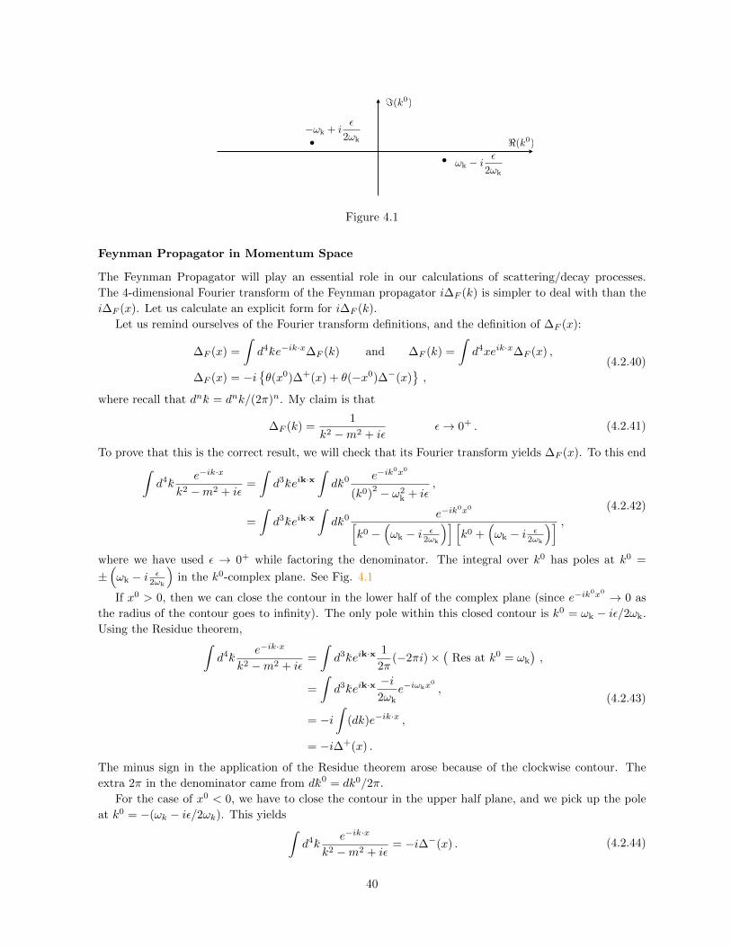
where we have used ε → 0+ while factoring the denominator. The integral over k0 has poles at k0 =
±(ωk − i ε
2ωk
)in the k0-complex plane. See Fig. 4.1
If x0 > 0, then we can close the contour in the lower half of the complex plane (since e−ik0x0 → 0 as
the radius of the contour goes to infinity). The only pole within this closed contour is k0 = ωk − iε/2ωk.
Using the Residue theorem,∫d4 −k
e−ik·x
k2 −m2 + iε=
∫d3 −keik·x
1
2π(−2πi)×
(Res at k0 = ωk
),
=
∫d3 −keik·x
−i2ωk
e−iωkx0
,
= −i∫
(dk)e−ik·x ,
= −i∆+(x) .
(4.2.43)
The minus sign in the application of the Residue theorem arose because of the clockwise contour. The
extra 2π in the denominator came from d−k0 = dk0/2π.
For the case of x0 < 0, we have to close the contour in the upper half plane, and we pick up the pole
at k0 = −(ωk − iε/2ωk). This yields∫d4 −k
e−ik·x
k2 −m2 + iε= −i∆−(x) . (4.2.44)
40
Putting the x0 > 0 and x0 < 0 results together, we have∫d4 −k
e−ik·x
k2 −m2 + iε= −iθ(x0)∆+(x) + θ(−x0)∆−(x) = ∆F (x) . (4.2.45)
This completes our proof. Note that the point of the iε was to guide us in the choice of poles to yield the
correct Fourier transform of the Feynman propagator.
Exercise 4.2.4 Consider a general(G) Green’s function of the Klein-Gordon equation: (∂2 +m2)∆G(x−y) = −δ(4)(x − y). Using the 4-d Fourier transform, show that ∆G(k) = 1/(k2 −m2). Now, start with
∆G(k) = 1/(k2 − m2), and try to get an explicit expression for ∆G(x − y) using the inverse Fourier
transform. You will be faced with a choice on how to evaluate the contour integral. The contour/pole
prescription we chose in Fig. 4.1 yields the Feynman Green’s function ∆F (x−y). What is the contour/pole-
prescription that is needed to recover the Retarded Green’s function ∆R(x− y)?
4.3 Perturbative Calculations in A Toy Model
Let us now put all of this technology to work in a toy example:
L = |∂ψ|2 −M2ψ†ψ +1
2(∂ϕ)2 − 1
2m2ϕ2 − gϕψ†ψ . (4.3.1)
where Hint = gϕψ†ψ, ϕ is a Hermitian field, and ψ a non-Hermitian one. Recall that for perturbative
calculations, we want g m,M . For convenience, I am going to write down the mode expansions for
these fields in the interaction picture (we have dropped the “I” denoting the interaction picture.)
ϕ(x) =
∫(dk)
(a(k)e−ik·x + a†(k)eik·x
),
ψ(x) =
∫(dk)
(b(k)e−ik·x + d†(k)eik·x
),
ψ†(x) =
∫(dk)
(d(k)e−ik·x + b†(k)eik·x
).
(4.3.2)
While far from reality, if it helps, you can think of ϕ particles as toy photons (γ) (they are really “toys”,
we will even allow them to have mass m), and ψ particles as toy electrons (e−) and positrons (e+). Again,
I want to stress that this is a toy example. Real world photons are quanta of spin 1, massless gauge fields
and electrons/positrons are quanta of spin 1/2 fermionic fields. Nevertheless, the essentials of perturbative
calculations will be present in our toy example without distractions (and more constraining structure) from
the higher spin fields.
Recall the following shorthand of the mode expansions, and their take-away:
• ϕ ∼ a+ a† : a† creates a γ, and a annihilates it.
• ψ ∼ b + d†, ψ† ∼ d + b† : d† creates an e+, and d annihilates it. Whereas b† creates a e−,
and b annihilates it.
Let us consider the amplitude for the following processes: (1) γ → e− + e+ (2) e− + e− → e− + e− (3)
e− + e+ → e− + e+ (4) e− + γ → e− + γ.
4.3.1 Decay: “γ”→ e− + e+
We will go through this calculation of the decay amplitude step by step, in excruciating detail. But having
done so once, the rest will hopefully be quicker.
41
e+
k1
k2
k3
e
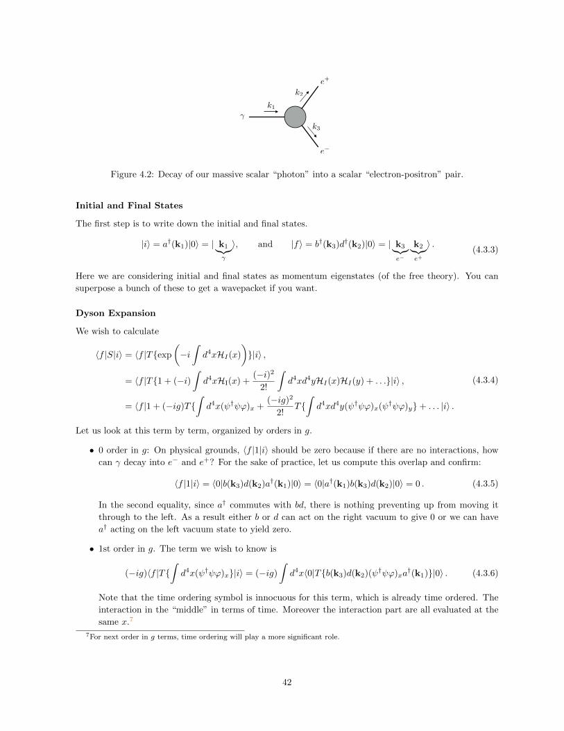
Figure 4.2: Decay of our massive scalar “photon” into a scalar “electron-positron” pair.
Initial and Final States
The first step is to write down the initial and final states.
|i〉 = a†(k1)|0〉 = | k1︸︷︷︸γ
〉, and |f〉 = b†(k3)d†(k2)|0〉 = | k3︸︷︷︸e−
k2︸︷︷︸e+
〉 .(4.3.3)
Here we are considering initial and final states as momentum eigenstates (of the free theory). You can
superpose a bunch of these to get a wavepacket if you want.
Dyson Expansion
We wish to calculate
〈f |S|i〉 = 〈f |Texp
(−i∫d4xHI(x)
)|i〉 ,
= 〈f |T1 + (−i)∫d4xHI(x) +
(−i)2
2!
∫d4xd4yHI(x)HI(y) + . . .|i〉 ,
= 〈f |1 + (−ig)T∫d4x(ψ†ψϕ)x +
(−ig)2
2!T∫d4xd4y(ψ†ψϕ)x(ψ†ψϕ)y+ . . . |i〉 .
(4.3.4)
Let us look at this term by term, organized by orders in g.
• 0 order in g: On physical grounds, 〈f |1|i〉 should be zero because if there are no interactions, how
can γ decay into e− and e+? For the sake of practice, let us compute this overlap and confirm:
〈f |1|i〉 = 〈0|b(k3)d(k2)a†(k1)|0〉 = 〈0|a†(k1)b(k3)d(k2)|0〉 = 0 . (4.3.5)
In the second equality, since a† commutes with bd, there is nothing preventing up from moving it
through to the left. As a result either b or d can act on the right vacuum to give 0 or we can have
a† acting on the left vacuum state to yield zero.
• 1st order in g. The term we wish to know is
(−ig)〈f |T∫d4x(ψ†ψϕ)x|i〉 = (−ig)
∫d4x〈0|Tb(k3)d(k2)(ψ†ψϕ)xa
†(k1)|0〉 . (4.3.6)
Note that the time ordering symbol is innocuous for this term, which is already time ordered. The
interaction in the “middle” in terms of time. Moreover the interaction part are all evaluated at the
same x.7
7For next order in g terms, time ordering will play a more significant role.
42
Contractions
Let us evaluate the following time-ordered vev using Wick’s theorem:
〈0|Tb(k3)d(k2)ψ†(x)ψ(x)ϕ(x)a†(k1)|0〉 = b(k3)d(k2)ψ†(x)ψ(x)ϕ(x)a†(k1) + b(k3)d(k2)ψ†(x)ψ(x)ϕ(x)a†(k1)
+ all possible contractions (with no non-contracted fields) .
where we have used Wick’s theorem for time ordered fields, and the fact that vevs of normal ordered fields
are 0. The types of contractions we have to deal with include
ϕ(x)a†(k1) = 〈0|Tϕ(x)a†(k1)|0〉 ,= 〈0|ϕ(x)a†(k1)|0〉,
=
∫(dq)e−iq·x〈0|a(q)a†(k1)|0〉 ,
=
∫(dq)e−iq·x〈0|a†(k1)a(q) + [a(q), a†(k1)]|0〉 ,
= e−ik1·x .
(4.3.7)
The second line is the innocuousness of time ordering for this term. The third line results from writing
down the mode expansion for ϕ(x); 〈0|a†(q) = 0 is why a†(q) does not appear in the expansion. In the
fourth line, we commuted a to the right past the a†, paying the price of doing so with the commutator.
Finally, in the fifth line, we used the commutation relation [a(q), a†(k1)] = 2ωk1δ(3)(q−k1) and integrated
w.r.t∫
(dq). Note that final result is in terms of the initial momentum k1 of the incoming particle.
Now note that contractions 〈0|Tϕaϕb|0〉 = ϕaϕb ∝ δab. Hence, if a 6= b (i.e different field), we get
no contribution. This implies that all contractions : ba, bϕ, dϕ, da,ϕψ and ψ†ϕ vanish. Moreover, since
ψ ∼ b+ d† and ψ† ∼ d+ b†, only bψ† and dψ survive. Thus the only surviving contributions are
〈0|Tb(k3)d(k2)ψ†(x)ψ(x)ϕ(x)a†(k1)|0〉 = b(k3)d(k2)ψ†(x)ψ(x)ϕ(x)a†(k1) ,
= 〈0|b(k3)ψ†(x)|0〉 × 〈0|d(k2)ψ(x)|0〉 × 〈0|ϕ(x)a†(k1)|0〉 ,= eik3·xeik2·xe−ik1·x .
(4.3.8)
Notice the sign difference between the incoming and outgoing momenta: k2, k3 are outgoing, whereas k1
is incoming.
The Matrix Elements
Thus we have arrived at
(−ig)〈f |T∫d4x(ψ†ψϕ)x|i〉 = (−ig)
∫d4xe−i(k3+k2−k1)·x = (−ig)δ(4)(k1 − k2 − k3) . (4.3.9)
Let us stop at this first nontrivial result which appears at first order in g (for dragons lurk at higher
orders). Combining this result with the 0th order result, we arrive at
〈f |S − 1|i〉 = (−ig)δ(4)(k1 − k2 − k3) +O[g2] . (4.3.10)
Recall from section 4.2.1 where we discussed properties of the S-matrix, that S = 1 − iδ(4)(pi − pf )Mwhere pi and pf are the 4-momenta of the initial and final states. The 4-dimensional delta function which
43
was meant to impose energy-momentum conservation in the process is precisely what we found in our
explicit calculation: δ(4)(k1 − k2 − k3). Thus, at leading order in g, we have
〈f |M|i〉 = g +O[g2] . (4.3.11)
An exceptionally simple result! The factors of i and signs were all put in (with hindsight) to make the
final results look nice.
4.3.2 Scattering: e− + e− → e− + e−
e
k3k1
k2 k4
e
ee
Figure 4.3: Scattering of two “electrons” off of each other.
Let us now calculate the amplitude for the following scattering process at the leading non-trivial order in
g. As with our decay calculation, we will proceed systematically, but now without loitering around for all
the details.
Initial and Final States
|i〉 = b†(k1)b†(k2)|0〉 = |k1k2〉 and |f〉 = b†(k3)b†(k4)|0〉 = |k3k4〉 , (4.3.12)
where we will assume that k1,k2 6= k3,k4.
Dyson Expansion
Since k1,k2 6= k3,k4, we immediately have 〈k3k4|k1k2〉 = 0. Hence we can directly write down the parts
of the scattering amplitude with g dependence:
〈k3k4|S − 1|k1k2〉
= (−ig)
∫d4x〈0|Tb(k3)b(k4)(ψ†ψϕ)xb
†(k1)b†(k2)|0〉
+(−ig)2
2!
∫d4xd4y〈0|Tb(k3)b(k4)(ψ†ψϕ)x(ψ†ψϕ)yb
†(k1)b†(k2)|0〉 ,
+O[g3] .
(4.3.13)
Contractions
Consider theO[g] term. It has an odd number of operators. Which means the time ordered vev. of these op-
erators will be zero. We must calculate theO[g2] term. Consider 〈0|Tb†(k3)b†(k4)(ψ†ψϕ)x(ψ†ψϕ)yb(k1)b(k2)|0〉.The number of possible complete contractions are enormous, but most will have vanishing contributions.
What sorts of contractions have non-vanishing contributions?
Note that any complete contraction with a non-vanishing contribution must include ϕ(x)ϕ(y) because
none of the other fields (including the initial and final states) contain any part of the ϕ field (recall that
ϕaϕb ∝ δab). Moreover, since ψ ∼ b + d† and ψ† ∼ d + b†, any b must contract with ψ† and b† with ψ.
There are four possible ways of doing this:
44
1.
b(k3)b(k4)ψ†(x)ψ(x)ϕ(x)ψ†(y)ψ(y)ϕ(y)b†(k1)b†(k2) .(4.3.14)
2. Same as 1., but with b(k3)ψ†(x)→ b(k3)ψ†(y), and b(k4)ψ†(y)→ b(k4)ψ†(x).
3. Same as 1., with x↔ y.
4. Same as 2., with x↔ y.
Let us take a closer look at individual two field contractions that appear in the above expressions.
• The ϕϕ contraction is nothing but the Feynman propagator:
ϕ(x)ϕ(y) = 〈0|Tϕ(x)ϕ(y)|0〉 = i∆ϕ(x− y) Feynman Propagator! (4.3.15)
• The ψ contraction with any (incoming) b† yields:
ψ(x)b†(kj) = e−ikj ·x incoming (4.3.16)
• The ψ† contraction with any (outgoing) b yields:
b(kj)ψ†(x) = eikj ·x outgoing (4.3.17)
Matrix Element
Using the above calculated building blocks,
〈k3k4|S − 1|k1k2〉 =(−ig)2
2!
∫d4xd4y i∆ϕ(x− y)
(eik3·xeik4·ye−ik1·xe−ik2·y + eik3·yeik4·xe−ik1·xe−ik2·y + x↔ y
)
The x ↔ y simply doubles the contribution, cancelling the 2! (this kind of stuff happens a lot). We end
up with
〈k3k4|S − 1|k1k2〉 = (−ig)2
∫d4xd4y i∆ϕ(x− y)
(e−i(k1−k3)·xe−i(k2−k4)·y + e−i(k1−k4)·xe−i(k2−k3)·y
).
(4.3.18)
This is the nontrivial part of the scattering amplitude at order O[g2]; we will get to higher order contri-
butions later.
I will take this opportunity to introduce one of the more elegant tools of QFT: Feynman Diagrams8
Julian Schwinger, one of the most prominent contributors to the development of QFT said:
“Like the silicon chips of more recent years, the Feynman diagram was bringing computation to the masses.”
Feynman Rules in x-space
There is powerful graphical way of representing the matrix element in eq. (4.3.18). Let me write down
x-space Feynman Rules for our theory in Fig. 4.4 Using these rules, we now depict the two terms in eq.
(4.3.18) as shown below in Fig. 4.5. Note that there is no accumulation of charge at the vertices. Let us
try to (heuristically) say in words what is going on in the process, and connect them to various parts of
the mathematical expression for the amplitude.
8For a gentle introduction to Feynman diagrams (suitable even if you have never taken field theory course), can be found at
http://www.quantumdiaries.org/2010/02/14/lets-draw-feynman-diagams/. If you are interested in the relevance of Feynman
diagrams in post WW2 era physics, see the book Drawing Theories Apart by D. Kaiser.
45
incoming
incoming e+
incoming eoutgoing e+
outgoing eeik·x =
(
outgoing
eik·x =
(
(ig)
Zd4x =
Time always flows from left to right. Arrows indicate the flow of positive charge.
external lines
internal lines
i'(x y) =
i (x y) =
vertex
Figure 4.4: x−space Feynman rules for our theory with Lint = −gψ†ψϕ.
k1
k2
k3
k4
x
y
k1
k2
k3
k4
+
x
y
Figure 4.5: The leading order O[g2] contribution to the e−+e− → e−+e− scattering amplitude: 〈k3k4|S−1|k1k2〉 = (−ig)2
∫d4xd4y i∆ϕ(x − y)
(e−i(k1−k3)·xe−i(k2−k4)·y + e−i(k1−k4)·xe−i(k2−k3)·y) represented in
terms of Feynman diagrams. Refer to the Feynman rules in x-space shown in Fig. 4.4 to see how the
elements of the diagrams correspond to different parts of the mathematical expression for the amplitude.
• “Electrons” with momenta k1 and k2 came in and exchanged a “photon”, and came out with momenta
k3 and k4.
• The integrals∫d4x and
∫d4y sums over all the locations x and y where the “photon” was exchanged.
• The propagator ∆ϕ(x− y) is symmetric in x and y and can be interpreted at the amplitude for the
“photon” going from x to y and y to x. This is internal (the “photon” is virtual), and cannot be
observed directly.
• The two diagrams are topologically distinct. You cannot twist and bend the lines to get from one to
another.
Doing calculations in x-space is fine, and sometimes necessary. Nevertheless, it is in Fourier space that
the calculations are the simplest.
Feynman Rules in k-space
We can simplify the expression for the matrix element significantly by writing down the Feynman propa-
gator in Fourier space: ∆ϕ(x− y) =∫d4 −ke−ik·(x−y)∆ϕ(k) to get
〈k3k4|S − 1|k1k2〉 = (−ig)2
∫d4xd4yd4 −k i∆ϕ(k)e−ik·(x−y)
(e−i(k1−k3)·xe−i(k2−k4)·y + e−i(k1−k4)·xe−i(k2−k3)·y
).
46
Now integrate over d4x and d4y to get a bunch of delta functions:
〈k3k4|S − 1|k1k2〉 = (−ig)2
∫d4 −k i∆ϕ(k)δ(4)(k1 − k3 + k)δ(4)(k2 − k4 − k) + δ(4)(k1 − k4 + k)δ(4)(k2 − k3 − k) ,
(4.3.19)
Once again, this expression can be depicted graphically using Feynman diagrams. Since the expressions
are in Fourier space, let me now provide the Feynman rules for our theory in k-space. Using these rules,
incoming
incoming e+
incoming eoutgoing e+
outgoing e
(
outgoing
(external lines
internal linesvertex
1 = 1 =
(ig)(4)(kin kout) =
Zd4k i'(k) =
Zd4k i (k) =
Figure 4.6: k−space Feynman Rules for our theory with Lint = −gψ†ψϕ.
the matrix element in eq. (4.3.19) can be represented again in terms of Feynman diagrams (see Fig. 4.7).
Two diagrams corresponds to the two terms in the expression for the matrix element. You can make the
correspondence by carefully looking at the delta functions.
k1
k2
k3
k4
k1
k2
k3
k4
+k k
Figure 4.7: The leading order O[g2] contribution to the e− + e− → e− + e− matrix element: 〈k3k4|S −1|k1k2〉 = (−ig)2
∫d4xd4yd4d4k i∆ϕ(k)e−ip·(x−y)
(e−i(k1−k3)·xe−i(k2−k4)·y + e−i(k1−k4)·xe−i(k2−k3)·y) rep-
resented in terms of Feynman diagrams. Refer to the Feynman rules in k-space shown in Fig. 4.6 to see
how the elements of the diagrams correspond to different parts of the mathematical expression for the
matrix element. Note that the choice of direction of the internal momentum k is arbitrary, you just have
to be consistent at both vertices once the direction is chosen.
We can even go further here. First note that the products of Dirac-delta functions appearing in eq.
(4.3.19) can be combined to yield a momentum conserving delta function that can be moved out of the
intergals:
〈k3k4|S − 1|k1k2〉 = (−ig)2δ4(k1 + k2 − k3 − k4)
∫d4 −k i∆ϕ(k)δ(4)(k1 − k3 + k) + δ(4)(k2 − k3 − k) ,
(4.3.20)
Now, recall that −iδ(4)(k1 + k2 − k3 − k4)〈k3k4|M|k1k2〉 = 〈k3k4|S − 1|k1k2〉, hence (finally!) the
interesting part of our matrix element for this scattering process at order g2 is
−i〈k3k4|M|k1k2〉 = (−ig)2
∫d4 −k i∆ϕ(k)δ(4)(k1 − k3 + k) + δ(4)(k2 − k3 − k) . (4.3.21)
47
Furthermore, since we know the form of the momentum-space propagator i∆ϕ(k) = i/(k2 − m2). The
martrix element then becomes
〈k3k4|M|k1k2〉 = g2
[1
(k1 − k3)2 −m2+
1
(k2 − k3)2 −m2
]. (4.3.22)
We will come back and relate this matrix element to cross section of scattering later. For the moment let
us continue calculating matrix elements for different types of scattering.
4.3.3 Scattering: e+ + e− → e+ + e−
k3k1
k2 k4
e e
e+e+
Figure 4.8: “electron”-“positron” scattering.
We will once again carry out the following steps. (1) Write down the initial and final states in terms of
creation and annihilation operators of the free fields. (2) Write down the Dyson expansion for the relevant
matrix element, and expand to the required non-trivial order in g. (3) Use Wick’s theorem; write down
the relevant contractions. (4) Write down the expression for the matrix element in position and Fourier
space.
Initial and Final States
|i〉 = b†(k1)d†(k2)|0〉 = | k1︸︷︷︸e−
k2︸︷︷︸e+
〉 and |f〉 = b†(k3)d†(k4)|0〉 = | k3︸︷︷︸e−
k4︸︷︷︸e+
〉 ,(4.3.23)
where for simplicity, we will assume k1,k2 6= k3,k4.
Dyson Expansion
The part of the scattering amplitude with g dependence (note that the O[g] term is zero):
〈k3k4|S − 1|k1k2〉 =(−ig)2
2!
∫d4xd4y〈0|Tb(k3)d(k4)(ψ†ψϕ)x(ψ†ψϕ)yb
†(k1)d†(k2)|0〉 +O[g3] .
(4.3.24)
Contractions
〈0|Tb(k3)d(k4)(ψ†ψϕ)x(ψ†ψϕ)yb†(k1)d†(k2)|0〉
= b(k3)d(k4)(ψ†ψϕ)x(ψ†ψϕ)yb†(k1)d†(k2) + x↔ y
+ b(k3)d(k4)(ψ†ψϕ)x(ψ†ψϕ)yb†(k1)d†(k2) + x↔ y
(4.3.25)
48
Note that ϕϕ contraction is essential since the |i〉 and |f〉 do not contain and a, a†. We cannot have any
ψ†ψ or ψψ contractions because the operators in |i〉 and |f〉 do not yield any non-zero contractions for
|i〉 6= |f〉.9
Matrix Element and Feynman Diagrams
Evaluating the expressions for the surviving contractions, we have
〈k3k4|S − 1|k1k2〉 = (−ig)2
∫d4xd4y i∆ϕ(x− y)
(e−i(k1+k2)·yei(k3+k4)·x + e−i(k1−k3)·ye−i(k2−k4)·x
).
(4.3.26)
Using our Feynman rules, we find that the two terms can be expressed graphically as follows: We can
k1
k2
k3
k4
xy
k1
k2
k3
k4
+
x
y
Figure 4.9: The leading order O[g2] contribution to the e− + e+ → e− + e+ scattering amplitude:
〈k3k4|S − 1|k1k2〉 = (−ig)2∫d4xd4y i∆ϕ(x − y)
(e−i(k1+k2)·yei(k3+k4)·x + e−i(k1−k3)·ye−i(k2−k4)·x) rep-
resented in terms of Feynman diagrams. Refer to the Feynman rules in x-space shown in Fig. 4.4 to see
how the elements of the diagrams correspond to different parts of the mathematical expression for the
amplitude.
repeat the calculation in momentum space, to get
〈k3k4|S − 1|k1k2〉
= (−ig)2
∫d4 −k i∆ϕ(k)
(δ(4)(k1 + k2 − k)δ(4)(k − k3 − k4) + δ(4)(k1 + k − k3)δ(4)(k2 − k − k4)
).
(4.3.27)
Once again, we may represent these terms in terms of Feynman diagrams in momentum space as shown
in Fig. 4.10.
k1
k2
k3
k4
k1
k2
k3
k4
+k
k
Figure 4.10: The leading order O[g2] contribution to the e− + e+ → e− + e+ matrix element: 〈k3k4|S −1|k1k2〉 = (−ig)2
∫d4k i∆ϕ(k)
(δ(4)(k1 + k2 − k)δ(4)(k − k3 − k4) + δ(4)(k1 − k3 − k)δ(4)(k2 − k − k4)
)
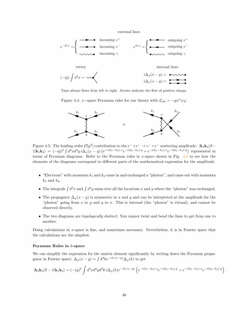
represented in terms of Feynman diagrams. Refer to the Feynman rules in k-space shown in Fig. 4.6
to see how the elements of the diagrams correspond to different parts of the mathematical expression for
the matrix element. Note that the choice of direction of the internal momentum k is arbitrary.
The expression for the scattering amplitude, can be simplified further. First, note that the products
of delta functions yield the usual momentum conserving delta function for the process. Using S = 1 −9If writing down these contractions gives you a bit of a headaches, be patient for a bit. We will soon get away from its
clutches.
49
iδ(4)(pi − pf )M, we have
〈k3k4|M|k1k2〉 = g2
∫d4 −k ∆ϕ(k)
(δ(4)(k − k1 − k2) + δ(4)(k1 − k3 − k)
),
= g2
(1
(k1 + k2)2 −m2+
1
(k1 − k3)2 −m2
).
(4.3.28)
Exercise 4.3.1 : Consider the following scattering process: γ + e− → γ + e−. Following the same route
as in the examples above: (1) Write down the initial and final states in terms of creation and annihilation
operators of the free fields. (2) Write down the Dyson expansion for the relevant matrix element, and
expand to the required non-trivial order in g. (3) Use Wick’s theorem; write down the relevant contractions.
(4) Write down the expression for the matrix element in position and Fourier space. Draw and label the
relevant Feynman diagrams in position and momentum space.
4.3.4 The Diagrammar’s way
So far, we have just noted that the final expressions for the scattering amplitude can be nicely represented
in terms of Feynman diagrams, but we have really not taken advantage of the graphical representation.
Indeed the power of Feynman diagrams lies in going the other way: draw diagrams, and the diagrams tell
you how to organize your calculations and compute amplitudes.10
Let me carry out this process for the theory under consideration: L = |∂ψ|2 −M2ψ†ψ + (1/2)(∂ϕ)2 −(1/2)m2ϕ2 − gϕψ†ψ. with Lint = −gϕψ†ψ. It is (typically) easiest to work in momentum space.
1. We will associate squiggly lines with ϕ and solid lines with ψ,ψ† (see Fig. 4.6). When they are
external, they contribute 1 to the amplitude.
2. Consider the free part of the theory (without Lint = 0). The information about this theory is
contained in it’s Green’s functions, or the transition amplitude. Calculate these, to get:
i∆ϕ(k) = i/(k2 −m2 + iε) and i∆ψ(k) = i/(k2 −M2 + iε) (4.3.29)
For internal line of ϕ contributes∫d4 −ki∆ϕ(k), whereas of ψ,ψ† contributes
∫d4 −ki∆ψ(k).
3. The interaction part of the Lagrangian density gives you the strength of the vertex: the three fields
represent the coming together of three different lines (ϕ,ψ, ψ†). This is your fundamental vertex.
This is the only possible way in which different lines in your diagram can meet. Construct the
contribution to the
3-point vertex = i∂3Lint
∂ψ∂ψ†∂ϕ× δ(4)(Σk) = (−ig)δ(4)(Σk) (4.3.30)
where the sum is over the momenta meeting at the vertex (by convention, incoming are given a
positive sign). Each vertex in the diagram will contribute a factor of g.
4. Now consider the process you are interested in. Say, for example e−(k1) + e+(k2)→ e−(k3) + e+(k4)
with all momenta being distinct. To calculated the amplitude, draw all possible topologically distinct
diagrams (up to the order of g you care about, which will fix the number of vertices allowed) with
the external momenta fixed (endpoints pinned down). If you can get from one diagram to another
10For a defense of “diagrams first” approach, read the introduction to Diagrammar by t’Hooft and Veltman. A recent
treatment along these lines is nicely presented in the introduction(s) of QFT I notes by Mojzis.
50
by twisting, but not cutting lines, then the diagrams are the same. (Note: There are annoying
combinatorial factors that come with the diagrams in many cases, but we are safe here for the model
under consideration). Now, we will draw all diagrams for the process of interest using the above
rules. Up to O[g2], we can have the following diagrams shown in Fig. 4.11. Once you have drawn
the diagrams, write down the integral expressions corresponding to the diagrams, and you are done
calculating the amplitude up to that order in g.
k3k1
k2 k4
e e
e+e+
= + + O[g4]
We will once again carry out the following steps. (1) Write down the initial and final states in terms of
creation and annihilation operators of the free fields. (2) Write down the Dyson expansion for the relevant
matrix element, and expand to the required non-trivial order in g. (3) Use Wick’s theorem; write down
the relevant contractions. (4) Write down the expression for the matrix element in position and Fourier
space.
Initial and Final States
|ii = b†(k1)d†(k2)|0i = | k1|z
e
k2|ze+
i and |fi = b†(k3)d†(k4)|0i = | k3|z
e
k4|ze+
i ,(4.3.23)
where for simplicity, we will assume k1,k2 6= k3,k4.
Dyson Expansion
The part of the scattering amplitude with g dependence (note that the O[g] term is zero):
hk3k4|S 1|k1k2i =(ig)2
2!
Zd4xd4yh0|Tb(k3)d(k4)(
† ')x( † ')yb†(k1)d†(k2)|0i + O[g3] .
(4.3.24)
Contractions
h0|Tb(k3)d(k4)( † ')x( † ')yb†(k1)d
†(k2)|0i
= b(k3)d(k4)( † ')x( † ')yb†(k1)d
†(k2) + x $ y
+ b(k3)d(k4)( † ')x( † ')yb†(k1)d
†(k2) + x $ y
(4.3.25)
Note that '' contraction is essential since the |ii and |fi do not contain and a, a†. We cannot have any
† or contractions because the operators in |ii and |fi do not yield any non-zero contractions for
|ii 6= |fi.7
Matrix Element and Feynman Diagrams
Evaluating the expressions for the surviving contractions, we have
hk3k4|S 1|k1k2i = (ig)2Z
d4xd4y iF (x y)ei(k1+k2)·yei(k3+k4)·x + ei(k1k3)·yei(k2+k4)·x
.
(4.3.26)
Using our Feynman rules, we find that the two terms can be expressed graphically as follows: We can
repeat the calculation in momentum space, to get
hk3k4|S 1|k1k2i
= (ig)2Z
d4 k iF (k)(4)(k1 + k2 k)(4)(k k3 k4) + (4)(k1 + k k3)
(4)(k2 k k4)
.
(4.3.27)
Once again, we may represent these terms in terms of Feynman diagrams in momentum space as shown
in Fig. 4.10.
The expression for the scattering amplitude, can be simplified further. First, note that the products
of delta functions yield the usual momentum conserving delta function for the process. Using S = 1 7If writing down these contractions gives you a bit of a headaches, be patient for a bit. We will soon get away from its
clutches.
18
We will once again carry out the following steps. (1) Write down the initial and final states in terms of
creation and annihilation operators of the free fields. (2) Write down the Dyson expansion for the relevant
matrix element, and expand to the required non-trivial order in g. (3) Use Wick’s theorem; write down
the relevant contractions. (4) Write down the expression for the matrix element in position and Fourier
space.
Initial and Final States
|ii = b†(k1)d†(k2)|0i = | k1|z
e
k2|ze+
i and |fi = b†(k3)d†(k4)|0i = | k3|z
e
k4|ze+
i ,(4.3.23)
where for simplicity, we will assume k1,k2 6= k3,k4.
Dyson Expansion
The part of the scattering amplitude with g dependence (note that the O[g] term is zero):
hk3k4|S 1|k1k2i =(ig)2
2!
Zd4xd4yh0|Tb(k3)d(k4)(
† ')x( † ')yb†(k1)d†(k2)|0i + O[g3] .
(4.3.24)
Contractions
h0|Tb(k3)d(k4)( † ')x( † ')yb†(k1)d
†(k2)|0i
= b(k3)d(k4)( † ')x( † ')yb†(k1)d
†(k2) + x $ y
+ b(k3)d(k4)( † ')x( † ')yb†(k1)d
†(k2) + x $ y
(4.3.25)
Note that '' contraction is essential since the |ii and |fi do not contain and a, a†. We cannot have any
† or contractions because the operators in |ii and |fi do not yield any non-zero contractions for
|ii 6= |fi.7
Matrix Element and Feynman Diagrams
Evaluating the expressions for the surviving contractions, we have
hk3k4|S 1|k1k2i = (ig)2Z
d4xd4y iF (x y)ei(k1+k2)·yei(k3+k4)·x + ei(k1k3)·yei(k2+k4)·x
.
(4.3.26)
Using our Feynman rules, we find that the two terms can be expressed graphically as follows: We can
repeat the calculation in momentum space, to get
hk3k4|S 1|k1k2i
= (ig)2Z
d4 k iF (k)(4)(k1 + k2 k)(4)(k k3 k4) + (4)(k1 + k k3)
(4)(k2 k k4)
.
=(ig)2Z
d4 k iF (k)(4)(k1 + k2 k)(4)(k k3 k4) + (ig)2Z
d4 k iF (k)(4)(k1 + k k3)(4)(k2 k k4)
(4.3.27)
Once again, we may represent these terms in terms of Feynman diagrams in momentum space as shown
in Fig. 4.10.
7If writing down these contractions gives you a bit of a headaches, be patient for a bit. We will soon get away from its
clutches.
18
k1
k2
k3
k4
k
k1
k2
k3
k4
k
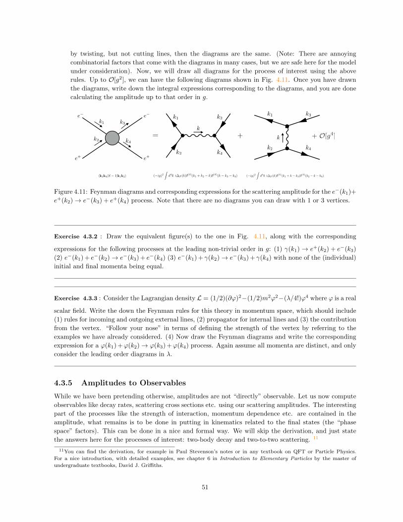
Figure 4.11: Feynman diagrams and corresponding expressions for the scattering amplitude for the e−(k1)+
e+(k2)→ e−(k3) + e+(k4) process. Note that there are no diagrams you can draw with 1 or 3 vertices.
Exercise 4.3.2 : Draw the equivalent figure(s) to the one in Fig. 4.11, along with the corresponding
expressions for the following processes at the leading non-trivial order in g: (1) γ(k1)→ e+(k2) + e−(k3)
(2) e−(k1) + e−(k2)→ e−(k3) + e−(k4) (3) e−(k1) + γ(k2)→ e−(k3) + γ(k4) with none of the (individual)
initial and final momenta being equal.
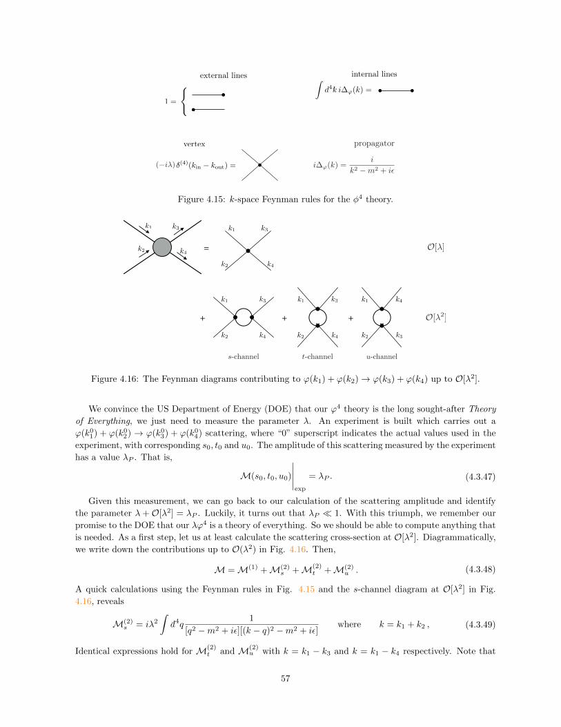
Exercise 4.3.3 : Consider the Lagrangian density L = (1/2)(∂ϕ)2−(1/2)m2ϕ2−(λ/4!)ϕ4 where ϕ is a real
scalar field. Write the down the Feynman rules for this theory in momentum space, which should include
(1) rules for incoming and outgoing external lines, (2) propagator for internal lines and (3) the contribution
from the vertex. “Follow your nose” in terms of defining the strength of the vertex by referring to the
examples we have already considered. (4) Now draw the Feynman diagrams and write the corresponding
expression for a ϕ(k1) +ϕ(k2)→ ϕ(k3) +ϕ(k4) process. Again assume all momenta are distinct, and only
consider the leading order diagrams in λ.
4.3.5 Amplitudes to Observables
While we have been pretending otherwise, amplitudes are not “directly” observable. Let us now compute
observables like decay rates, scattering cross sections etc. using our scattering amplitudes. The interesting
part of the processes like the strength of interaction, momentum dependence etc. are contained in the
amplitude, what remains is to be done in putting in kinematics related to the final states (the “phase
space” factors). This can be done in a nice and formal way. We will skip the derivation, and just state
the answers here for the processes of interest: two-body decay and two-to-two scattering. 11
11You can find the derivation, for example in Paul Stevenson’s notes or in any textbook on QFT or Particle Physics.
For a nice introduction, with detailed examples, see chapter 6 in Introduction to Elementary Particles by the master of
undergraduate textbooks, David J. Griffiths.
51
Decay rate
For the decay of a particle with mass m1 (at rest) into two particles with masses m2 and m3, the decay
rate
Γ1→2+3 = S|k|
8πm21
|〈f |M|i〉|2 . (4.3.31)
where k = (2m1)−1√m4
1 +m42 +m4
3 − 2m21m
22 − 2m2
1m23 − 2m2
2m23 is the momentum of either outgoing
particle. The factor S is related to the number of identical particles in the final state. For our ϕψ†ψtheory and the case of γ → e+ + e−, we have S = 1 (if they were identical S = 1/2!). The outgoing
momenta |k| =√m2 − 4M2. Hence
Γγ→e+e− =g2
16πm
√1− 4M2
m2(4.3.32)
Note that m > 2M is necessary for decay, as expected (ϕ clearly is not the electromagnetic field!). In the
limit that M m, we have Γ ≈ g2/8πm.
Differential cross-section
Now let us consider a 1 + 2→ 3 + 4 scattering in the center of momentum frame (k1 = −k2,k3 = −k4).
The differential cross-section (cross-section per unit solid-angle for the outgoing particles),(dσ
dΩ
)
1+2→3+4
=S
(8π)2
|〈f |M|i〉|2(ωk1
+ ωk2)2
|kf ||ki|
(4.3.33)
where ωk1and ωk2
are the energies of the incoming particles, |kf | is the magnitude of the 3-momentum of
either outgoing particle and |ki| is the magnitude of either incoming particle. For our ϕψ†ψ theory, and
for the particular case of e+ + e− → e+ + e− scattering, we have |kf | = |ki|, and the formula simplifies to(dσ
dΩ
)
e+e−→e+e−=
1
64π2
|〈f |M|i〉|2E2
cm
(4.3.34)
where we used (k1 + k2)2 = (ωk1+ ωk2
)2 = E2cm which is (the square of) the energy of the system in the
center of momentum frame. Recall, that we calculated 〈f |M|i〉 for this process in eq. (4.3.28). Thus we
have (dσ
dΩ
)
e+e−→e+e−=
g4
64π2E2cm
(1
E2cm −m2
− 1
2|kf |2(1− cos θ) +m2
)2
. (4.3.35)
The angle θ is the angle between the initial and final (back to back) particle trajectories in the center
of momentum frame. Notice the first term inside the brackets has a denominator which goes to zero at
Ecm → m. Thus the cross section diverges (in reality, it will rise and fall fast) near Ecm = m as we scan
through Ecm. This sharp rise and fall reveals the presence of a particle of mass m as the means by which
the interaction between our e+ and e− (mass M each) takes place! Note that if 2M > m, then there is no
“resonance” possible.
As we have seen from the calculation of amplitudes, the Lorentz invariant combinations s = (k1 +k2)2,
t = (k1 − k3)2 and u = (k1 − k4)2 appear quite naturally. These are called Mandelstam variables. They
have nice interpretations. For example,√s is the center of momentum energy and t and u are related
to momentum transfer. In terms of the Mandelstam variables, that the amplitude for the e+e− → e+e−
scattering (see eq. (4.3.28)) can be written as
〈k3k4|M|k1k2〉 = g2
(1
s−m2+
1
t−m2
)(4.3.36)
The process related to the diagrams contributing these pieces would be called s-channel (first diagram in
Fig. 4.10), and t-channel (second diagram in Fig. 4.10) process respectively.
52
Amplitudes and cross-sections to forces
Consider the e−(k1) + e+(k2)→ e−(k3) + e+(k4) process; the differential cross-section is given by
dσ
dΩ=
g4
64π2s
(1
s−m2+
1
t−m2
)2
. (4.3.37)
Let us focus on the non-relativistic limit (that is, |kj | M) and restrict ourselves to the case where
mM . In this case kj ≈ (M,kj). Hence, s ≈ 4M2, t = −|k1 − k3|2 ≡ −|q|2 where q is the momentum
transfer anddσ
dΩ≈ g4
256π2M2
(1
|q|2 +m2
)2
. (4.3.38)
Let us now consider the same problem e−(k1) + e+(k2)→ e−(k3) + e+(k4) in non-relativistic quantum
mechanics. We imagine that e+ and e− interact via a potential V (x) where x is their separation vector.
The Born-approximation, then tells us that the scattering amplitude from a momentum eigenstate |ki〉 to
|kf 〉 is 〈kf |V (x)|ki〉 ∝∫d3xV (x)e−i(ki−kf )·x, and the differential cross section
dσ
dΩ∝∣∣∣∣∫d3xV (x)e−iq·x
∣∣∣∣2
=∣∣∣V (q)
∣∣∣2
, (4.3.39)
where q is ki−kf , ie. it is the momentum transfer and V (q) is the Fourier transform of V (x). Comparing
eq. (4.3.39) and eq. (4.3.37), we see that
V (q) ∝ 1
|q|2 +m2=⇒ V (x) ∝ e−m|x|
|x| . (4.3.40)
If this is the interaction potential, the force will be F = −∇V (x). Thus we have discovered that the force
between our “electron” and “positron” due to the exchange of a scalar particle of mass m is given by
|F| ∝
1/|x|2 |x| m−1
e−m|x|/|x| |x| m−1(4.3.41)
That is, we have a “1/r2” force for distances small compared to m−1 and a “Yukawa screening” for
distances large compared to m−1!12
Exercise 4.3.4 (i) Verify that in the non-relativistic limit, and with m M , eq. (4.3.37) leads to eq.
(4.3.38). (ii) Then verify the implication in eq. (4.3.40) (ie. calculate the Fourier transform). (ii) Sketch
V (x) as a function of |x| on a log-log plot. (iv) From the dynamics of the inner planets in our solar
system13, one finds that force law is “1/r2” (or more correctly, consistent with general relativity which
has massless gravitons) at order O(10−8). Using our Yukawa type potential to parametrize the effect of a
massive graviton, what is the constraint on the mass of the graviton mg? (give your answer in eV). Order
of magnitude is fine, but explain your reasoning. What is the length scale in meters corresponding to this
mass?
12It is worth noting that if we kept track of signs, we would find an attractive force regardless of whether we consider e+e−
or e−e− scattering. Scalar exchange in our theory yields an attractive force. We have to go to Quantum Electrodynamics,
the correct theory for electrons, positrons and photons to see that like charges repel, and unlike charges attract. The spin
of the force carrier matters! Electrodynamics has a (massless) spin-1 carrier, and gravity, a (massless) spin-2 carrier which
determine whether we can have attractive/and or repulsive forces.13Note that 1AU ≈ 1.5× 10¹¹ meters, which you can take as the typical size of orbits of inner planets
53
4.3.6 Beyond Leading Order
Connected and Amputated Contributions
So far we have always calculated amplitudes at the leading order in the coupling constant. For example,
the amplitude for e−+ e− → e−+ e− scattering, we calculated the matrix element 〈f |S− 1|i〉 to order g2.
What happens if we want to calculate amplitudes beyond the leading order. Following the “Diagrammer’s
way”, let us try to draw the diagrams at next order in g, making use of the fundamental vertex. I will be a
bit sloppy, and ignore the arrows on the ψ,ψ† lines, not label external momenta and also not draw diagrams
that can be obtained by permutations of external legs, rotation from one to the other etc. We have the
following diagrams (shown in Fig. 4.12). Each diagram will have an expression associated with (which can
be written down using our Feynman rules), which when added together should yield the total amplitude.
Take a close look. Some parts of the diagrams (for example the one inside (. . .)) are disconnected from the
external lines. They are ”vacuum bubbles”. You can convince yourself that you can factor the diagrams
into a product of connected diagrams and disconnected vacuum bubbles.14
+ + + + ++
+
=
+ + + . . . + + + . . .+...
= + + + + + . . .1 +
vacuum ! vacuum
+ + +O[g6]+
Figure 4.12: The diagrammatic expansion of the amplitude for e−e− → e−e−. Note the factorization of
the vacuum bubbles in the last line. Permutations of external legs has been ignored for simplicity.
The pieces with the vacuum bubbles can be thought of as contributing to the vacuum-to-vacuum
transition. Since we normalize the vacuum, this means that at best contribution from the bubbles is a
phase eiθ, and does not influence the overall scattering probability density (|eiθ|2 = 1).15
Now look at diagrams with “loops” on external legs. It turns out that we can amputate these legs (for
example, cut before the loop begins on the outgoing external legs, or cut after the loop for the incoming
external legs). Why is this physically reasonable? This is ok, because as you might recall, we used free-field
initial and final states. The external legs with loops is just correcting for the initial and final states in the
full theory, and do not have anything to do with the scattering itself. So, with these two rules, we can
simplify our scattering calculation as follows:
〈f |S − 1|i〉 =∑
(All connected, amputated Feynman diagrams) (4.3.42)
14Our simplifying assumption that the external momenta are not equal precludes disconnected diagrams with external
legs.15I am being a bit sloppy here about whether I am talking about the interacting vacuum or the non-interacting vacuum
and such. You can look at, for example, Ch. 22 of QFT for the Gifted Amateur
54
+ + + + ++
+
=
+ + + . . . + + + . . .+...
= + + + + + . . .1 +
vacuum ! vacuum
+ + +O[g6]
= + +
+
+ + + + . . .+
connected and amputated diagramsFigure 4.13: The diagrammatic expansion, including only the connected amputated diagrams, of the
amplitude for e−e− → e−e− scattering.
You will find it useful to revisit the Gell-Mann-Low theorem (see eq. (4.2.16)) to see if using connected
Feynman diagrams make sense. For example, the denominator is the vacuum to vacuum transition, which
precisely cancels the disconnected vaccum bubble contributions from the numerators. The factor of Z in
the LSZ reduction formula (see eq. (4.2.15)) can take care of the amputated part.
Divergences at higher orders
k1
k2
k3
k4
k
r
p q
Figure 4.14: The diagrammatic expansion, including only the connected amputated diagrams, of the
amplitude for e−e− → e−e− scattering.
Let us focus on one of the diagrams at O[g4] in the for e−e− → e−e− process discussed above (see
Fig. 4.14, and try to calculate the integral corresponding to this diagram). Following the Feynman rules
in Fig. 4.6, we have
〈f |S − 1|i〉 =(−ig)4
∫−d4k −d4p −d4q −d4r i∆ϕ(k) i∆ϕ(r) i∆ψ(p) i∆ψ(q)
× δ(4)(k1 + k − k3)δ(4)(q − p− k)δ(4)(r − q + p)δ(4)(k2 − r − k4) ,
= (−ig)4δ(4)(k1 + k2 − k3 − k4) i∆ϕ(k1 − k3) i∆ϕ(k2 − k4)
∫−d4q i∆ψ(q) i∆ψ(k1 − k3 + q)
︸ ︷︷ ︸internal loop
.
(4.3.43)
Using our expressions for the propagators in (4.3.29), we can write the contribution from the “internal
loop” as
I(k) =
∫−d4q
i
q2 −M2 + iε
i
(k + q)2 −M2 + iεk ≡ k1 − k3 . (4.3.44)
Roughly speaking, the integral measure yields q4, whereas the two propagators also yield q−4 as q →∞.
This scaling at large momenta indicates that the integral will diverge logarithmically at large q. This is
terrible news! The same is true for (some of) the even higher order diagrams. So the scattering amplitudes
have the form 〈f |S − 1|i〉 ∼ g2(finite) + g4(∞?) + . . . This means that the contributions to the amplitude
55
diverges at higher orders in g, and puts our entire scheme of perturbation in small g into question. What
did we miss ?
Exercise 4.3.5 : Consider the process γ(k1) + e+(k2) → γ(k3) + e+(k4). (a) Draw all connected and
amputated Feynman diagrams up to 4-th order in g. You can ignore permutations of external legs (and
no need to label the external momenta for this part). (b) Draw a diagram with a disconnected piece at
order g4. (c) Write down the expression corresponding to the “box” diagram O[g4] in (Similar, but not
identical to the 4-th diagram from the left after the = sign in Fig. 4.13) and simplify as much as you can.
Exercise 4.3.6 : Consider the process ϕ(k1)+ϕ(k2)→ ϕ(k3)+ϕ(k4) in the L = (1/2)(∂ϕ)2−(1/2)m2ϕ2−(η/3!)ϕ3 theory. (a) Write down the fundamental vertex in this theory in momentum space. (b) Draw
all connected and amputated Feynman diagrams up to 4rth order in η. You can ignore permutations of
external legs (and no need to label the external momenta for this part). (c) Draw a diagram corresponding
to an s-channel process at O[η2] and write down the expression corresponding to this diagram. Simplify
as far as possible. (d) Draw a diagram corresponding to an s-channel process at O[η4], with a bubble
on the inner propagator and write down the expression corresponding to this diagram. Simplify as far as
possible.
4.3.7 A Taste of Renormalization
At this point we need to turn to the important idea of renormalization, which provides an algorithm as well
as physical reasoning to remove these infinites. Powerful ideas such as the scale dependence of parameters
make an appearance. In this course we do not have time to discuss many aspects of renormalization in
detail. Nevertheless, these ideas are too important to skip over entirely, so let us try to do as much as we
can in simple examples. In what follows, I rely on A. Zee’s QFT in a Nutshell.
We encounter infinities in a scattering calculation in the ϕψ†ψ theory when we went beyond leading
order in perturbation theory (at least for some, though not necessarily all diagrams). Instead of dealing
with this theory (which while simple, still has too many ingredients), I am going to discuss renormalization
in an even simpler theory: a real, massive scalar field theory with a ϕ4 interaction. We consider the
following Lagrangian density for this theory
L =1
2(∂ϕ)2 − 1
2m2ϕ2 − λ
4!ϕ4 . (4.3.45)
Note that λ is dimensionless. To make our analysis as simple as possible, we assume that m is smaller
than any energy scale of interest where we conduct our scattering experiments. For technical reasons, it
is best to keep carrying along a really small, but still non-zero m. The Feynman rules for this theory are
straightforward enough, as seen in Fig. 4.15.
In this theory, let us consider the ϕ(k1) +ϕ(k2)→ ϕ(k3) +ϕ(k4) scattering. At leading order in λ, we
haveM(s, t, u) =M(1) +O[λ2] ,
= λ+O[λ2] ,(4.3.46)
where our M is really shorthand for 〈f |M|i〉 related to the scattering amplitude via 〈f |S − 1|i〉 =
−iδ(4)(pin− pout)〈f |M|i〉. Note that the “(n)” inM(n) is the order in λ and s = (k1 +k2)2, t = (k1−k3)2
and u = (k1 − k4)2 are the Mandelstam variables.
56
(external lines internal lines
vertex
1 =
(ig)(4)(kin kout) =
Zd4k i'(k) =
i'(k) =i
k2 m2 + i
propagator
(i)
Figure 4.15: k-space Feynman rules for the φ4 theory.
k3k1
k2 k4
k1 k3
k2 k4
k1 k3
k2 k4
k1 k3
k2 k4
k1
k3k2
k4
=
+ ++
O[]
O[2]
s-channel t-channel u-channel
Figure 4.16: The Feynman diagrams contributing to ϕ(k1) + ϕ(k2)→ ϕ(k3) + ϕ(k4) up to O[λ2].
We convince the US Department of Energy (DOE) that our ϕ4 theory is the long sought-after Theory
of Everything, we just need to measure the parameter λ. An experiment is built which carries out a
ϕ(k01) + ϕ(k0
2) → ϕ(k03) + ϕ(k0
4) scattering, where “0” superscript indicates the actual values used in the
experiment, with corresponding s0, t0 and u0. The amplitude of this scattering measured by the experiment
has a value λP . That is,
M(s0, t0, u0)
∣∣∣∣∣exp
= λP . (4.3.47)
Given this measurement, we can go back to our calculation of the scattering amplitude and identify
the parameter λ+O[λ2] = λP . Luckily, it turns out that λP 1. With this triumph, we remember our
promise to the DOE that our λϕ4 is a theory of everything. So we should be able to compute anything that
is needed. As a first step, let us at least calculate the scattering cross-section at O[λ2]. Diagrammatically,
we write down the contributions up to O(λ2) in Fig. 4.16. Then,
M =M(1) +M(2)s +M(2)
t +M(2)u . (4.3.48)
A quick calculations using the Feynman rules in Fig. 4.15 and the s-channel diagram at O[λ2] in Fig.
4.16, reveals
M(2)s = iλ2
∫−d4q
1
[q2 −m2 + iε][(k − q)2 −m2 + iε]where k = k1 + k2 , (4.3.49)
Identical expressions hold for M(2)t and M(2)
u with k = k1 − k3 and k = k1 − k4 respectively. Note that
57
integral
I(k) =
∫−d4q
1
[q2 −m2 + iε][(k − q)2 −m2 + iε], (4.3.50)
diverges logarithmically at large q! That is disheartening. So much for our theory of everything! The
divergence is coming from large q. Let us (at least momentarily) give up the belief that we our λϕ4 theory
is the complete theory, and make the reasonable assumption that we only know our theory to some large
energy/momentum scale Λ. We call this large but unknown Λ the cutoff scale of the theory. In that case,
we should only compute the integral up to the cutoff, that is,
IΛ(k) =
∫ Λ−d4q
1
[q2 −m2 + iε][(k − q)2 −m2 + iε],
=
∫−d4q
1
[q2 −m2 + iε][(k − q)2 −m2 + iε]− 1
[q2 − Λ2 + iε][(k − q)2 − Λ2 + iε]
.
(4.3.51)
The second equality is just one of the many possible ways of “regulating” the integral. This way of
making an infinite integral finite is called Pauli-Villars regularization. There are other ways of doing
this (for example, Dimensional regularization); regularization schemes should not affect observables in the
end. Note that for for q Λ, the integrand vanishes, whereas for q Λ the Λ dependent term will be
suppressed compared to the first by Λ−4. This integral IΛ(k) can now be evaluated (though not trivially
by any means). In the limit that k2 m2:
IΛ(k) = ia[ln Λ2 − ln s
]where s = (k1 + k2)2 = k2 m2 , (4.3.52)
and a is a constant. Using this expression for IΛ(k) and combining all the terms in the amplitude for
scattering (up to O[λ2], see eq. (4.3.48)), we have
M(s, t, u) = λ− aλ2[3 ln Λ2 − ln s− ln t− lnu
]+O[λ3] . (4.3.53)
where we have made the dependence on s, t and u explicit in M. This is not of much help. We still have
an unknown Λ in the problem. We know λ+O[λ2] = λP from eq. (4.3.47). But only to leading order. So
to get the amplitude at higher order in λ we have to figure out what λ is, along with the unknown Λ.
Recall that we have experimentally measured the scattering amplitude at (s, t, u) = (s0, t0, u0), and
found the experimental value to be λP (eq.(4.3.47)). Experimental results do not care about how we do
our calculations, or to what order in perturbation theory. A scattering amplitude was measured at some
value of incoming and outgoing momenta, and the answer is λP . This bit of information is very useful as
we now see. Evaluating eq. (4.3.53) at (s, t, u) = (s0, t0, u0) and comparing it with eq. (4.3.47), we have
λP = λ− aλ2[3 ln Λ2 − ln s0 − ln t0 − lnu0
]+O[λ3] . (4.3.54)
For finite Λ, we can invert this series, and since λP 1, we have
λ = λP + aλ2P
[3 ln Λ2 − ln s0 − ln t0 − lnu0
]+O[λ3
P ] (4.3.55)
Let us substitute this “improved” λ into our general expression eq. (4.3.53). We arrive at
M(s, t, u) = λP + aλ2P [ln(s/s0) + ln(t/t0) + ln(u/u0)] +O[λ3
P ] . (4.3.56)
Magic! This expression does not have the unknown Λ in it, and is written entirely in terms of known
quantities based on a previous measurement of M(s0, t0, u0)|exp = λP . With this expression we can now
compute the scattering amplitude for ϕ(k1) + ϕ(k2)→ ϕ(k3) + ϕ(k4) for any experiment ie. any s, t and
u up to O[λ2P ].
The lesson we learnt is that perturbation theory in terms of λ is a bit sick. It leads to divergences our
calculation of observables, or at least leads to a dependence on large unconstrained cutoff scale physics Λ.
58
However, if we express our answers in terms of physical coupling constants (ones measured in experiment),
then the divergences and cutoff dependences vanish! 16
In some cases, when we reach some high energy scale Λ in an experiment, we might discover new
physics that cures the divergence. Nevertheless, the above procedure shows that we do not need to know
the physics at Λ to make predictions at much lower energy scales. That should be a relief.
Flow of Physical Coupling Constants
Recall that λP = M(s0, t0, u0)|exp. Let us, for convenience, chose s0 = t0 = u0 = µ20. Note that
is impossible to actually do this for any k01, k
02, k
03, k
04, but this choice does not affect the subsequent
arguments. We interpret λP as the physical coupling constant measured at the energy scale µ0: λP (µ0).
Let us re-write M(s, t, u) expression above with a mildly simplified expression:
M(s, t, u) = λP (µ0) + aλ2P (µ0)
[ln(s/µ2
0) + ln(t/µ20) + ln(u/µ2
0)]
+O[λ3P ] . (4.3.58)
There is nothing special about µ0. We could equally have carried out the above procedure at another
energy scale µ1. Then
M(s, t, u) = λP (µ1) + aλ2P (µ1) [ln(s/µ1) + ln(t/µ1) + ln(u/µ1)] +O[λ3
P ] . (4.3.59)
Since the L.H.S M(s, t, u) in eqns. (4.3.58) and (4.3.59) are the same, we equate the two. Then, as
∆µ = µ1 − µ0 → 0, we get
dλP (µ)
d lnµ
∣∣∣∣∣µ=µ0
= 6aλ2P (µ0) +O[λ3
P ] (4.3.60)
Or more generally,dλP (µ)
d lnµ= 6aλ2
P (µ) +O[λ3P ] . (4.3.61)
This equation, now tells us how λP changes with the energy scale µ. The physical “coupling constant” is
not really a constant. If a is positive (which is the case for this theory), λP increases with µ, that is the
theory is becoming more strongly interacting at higher energies or equivalently, smaller length scales.
In a theory with a number of coupling constants λ0, λ1, . . . we will have
dλid lnµ
= βi(λ0, λ1 . . .) , (4.3.62)
where we have dropped the subscript “P” for physical coupling constant to avoid clutter. The βi are called
the Beta functions of the theory. The signs of the βi tell us about how the couplings flow with energy
µ. As you might imagine, the fixed points in this space of couplings (βi(λ?1, λ
?2 . . .) = 0) are particularly
special. 17
As a couple of physically relevant cases of interest, note that in Quantum Electrodynamics, the “physical
charge” of electronsd eP (µ)
d lnµ=
1
12π2e3P (µ) +O[e5
P ] . (4.3.63)
16Consider a more general low energy theory (compared to Λ) of the form
L =1
2(∂φ)2 −
1
2m2φ2 +
∑n≥3
λn
n!φn . (4.3.57)
Note that since the mass dimensions of L = 4 and [φ] = 1, we have [λn] = 4 − n. Here is some nomenclature. Terms with
[λn] < 0 are called relevant, terms with [λn] = 0 are called marginal, whereas terms with [λn] > 0 are called irrelevant. We
typically expect only marginal and relevant terms to contribute to our low energy (compared to Λ) processes. Moreover, it
turns out that theories with [λn] > 0 are not re-normalizable. However, that does not rule out such terms (just that our
theory will have a domain of validity in terms of energies).17Time permitting, we will discuss such a point in the context of current conduction in presence of impurities and Anderson
Localization in class.
59
As you probe electrons at higher and and higher energy scales, the charge gets larger and larger. On the
other hand, for Quantum chromodynamics, we find that
d gP (µ)
d lnµ< 0 ! (4.3.64)
The coupling gets weaker at higher energies. This is asymptotic freedom; quarks become free at high
energies but are strongly bound into mesons and hadrons at low energies.
There is a lot more to learn regarding renormalization. Will we always be able to get rid of the cutoff?
What about higher order terms? How do we do all this systematically? We unfortunately have to move
on, but hopefully I have given you some flavor of how some of the infinities can be dealt with. For a more
in-depth, but still accessible view see A. Zee’s textbook. You might also want to consult QFT for the
Gifted Amateur as well as notes on renormalization by M. Luty. ,
Exercise 4.3.7 : Learn about “Feynman Parametrization” of integrals and “Dimensional Regularization”
on your own. Now evaluate the non-divergent, energy dependent and part of the integral in eq. (4.3.50)
at 0th order in the dimensional regularization parameter (ie. the finite part that remains as you take the
dimensional regularization parameter to 0). You can leave your answer in terms of the integral over the
Feynman parameter, or evaluate it explicitly if you can.
4.4 Summary
Let me graphically summarize all that we have done so far for weakly interacting scalar fields:
Lagrangian
free part interaction
mode expansionpropagator vertex
Feynman Rules [or Dyson expansion]
amplitudes (tree level)
(higher order — Renormalization)
Figure 4.17: Summary of the course so far: QFT for weakly interacting scalar fields.
60
CHAPTER 5
SYMMETRY AND FIELDS
5.1 Spacetime and Internal Symmetries
Consider the action
S =
∫d4xL(ϕa, ∂µϕa) , (5.1.1)
where a = 1, 2 . . . N , and ϕa are N scalar fields, or N components of some field. First, let us recall precisely
what we mean by symmetries.
A symmetry transformation is an operation that does not change the action. Such a transformation
must then change the Langrangian density by at most a total derivative:
L = L+ ∂µFµ , (5.1.2)
where Fµ(x) are 4 arbitrary functions of spacetime. Moreover, a continuous symmetry transformation
means that we are allowed to work with infinitesimal transformations.
Let us make this concrete with an exceptionally simple example. Consider the Lagrangian density
of a complex scalar field L = |∂ψ|2 − M2|ψ|2 − λ|ψ|4, and the corresponding action S =∫d4xL. A
transformation which rotates the field in the complex plane by the same constant angle α everywhere,
ie. ψ(x) = eiαψ(x) is a symmetry transformation, since it leaves the Lagrangian density (and the action)
unchanged. Since the result holds for arbitrarily small α, it is also a continuous symmetry transformation
(ψ(x) = ψ + δψ = ψ + iαψ for small α). For the same Lagrangian, a Lorentz transformation is also a
continuous symmetry transformation. It would generate non-zero ∂µFµ terms.
5.1.1 Noether’s Theorem and its Consequences
Noether’s Theorem: Every continuous symmetry of the action yields a current jµ which is conserved
via the equations of motion.
Proof: Consider an infinitestimal transformation which changes the fields as follows: ϕa = ϕa+δϕa. Then
61
under this transformation, the Lagrangian density changes as follows
δL =
N∑
a=1
(∂L∂ϕa
δϕa +∂L
∂(∂µϕa)∂µ(δϕa)
),
=
N∑
a=1
[∂L∂ϕa
− ∂µ(
∂L∂(∂µϕa)
)]
︸ ︷︷ ︸= 0 if ϕa satisfies the EOM
δϕa +
N∑
a=1
∂µ
[∂L
∂(∂µϕa)δϕa
],
=
N∑
a=1
∂µ
[∂L
∂(∂µϕa)δϕa
],
(5.1.3)
Note that we have used that ϕa satisfies the equation of motion. If this transformation is a symmetry
transformation, then we must have δL = ∂µFµ (see eq. (5.1.2)). Combining with our result above for δL,
we have
∂µFµ =
N∑
a=1
∂µ
[∂L
∂(∂µϕa)δϕa
]=⇒ ∂µ
[N∑
a=1
∂L∂(∂µϕa)
δϕa − Fµ]
= 0 . (5.1.4)
Thus, we have just constructed a current
jµ ≡N∑
a=1
∂L∂(∂µϕa)
δϕa − Fµ , such that ∂µjµ = 0 on the the eq. of motion . (5.1.5)
The “on the eq. of motion” part refers to the fact that ϕa satisfies the eq. of motion. This completes
the proof of Noether’s theorem. While not evident right now, Fµ will be obtained by finding δL (which is
a scalar) for any particular symmetry transformation without using the expression for L in terms of the
fields.
All this might might seem a bit abstract. We will make Noether’s theorem and its implications more
concrete by considering examples of continuous symmetries. But before moving on to concrete, physically
relevant examples, a few comments are in order:
• Conserved Charge: Note that
∂µjµ = 0 =⇒ ∂0j
0 = −∇ · j ,
=⇒ ∂0
∫d3xj0 = −
∫d3x∇ · j ,
=⇒ Q = −∫
j · dS = 0 where Q ≡∫d3xj0 .
(5.1.6)
where in the last line we defined a charge Q and assumed that j vanishes sufficiently rapidly at spatial
infinities. Noether’s theorem points to the existence of a conserved charge for every continuous
symmetry transformation.
• It is convenient to define a momentum density πµa , so that
jµ =
N∑
a=1
πµa δϕa − Fµ with πµa ≡∂L
∂(∂µϕa). (5.1.7)
• Charges as generators of symmetries: It is useful to think of Q as a generator of symmetries
62
in the following way. Consider the Poisson bracket of Q with the field ϕa:
Q,ϕa = ∫d3x
N∑
b=1
π0bδϕb − F 0, ϕa ,
=
∫d3x
N∑
b=1
π0b , ϕaδϕb ,
= −δϕa .
(5.1.8)
where in the the third line we assumed that δϕa and F 0 do not depend on π0a.1 Thus we have
δϕa = −Q,ϕa. It is in this sense that Q generates the symmetry transformation.
• While all the above statements have been made for classical fields, the arguments carry over to
quantum fields with f → f , and with ·, · → −i[·, ·]. In particular
δϕa = i[Q, ϕa] , (5.1.9)
and Q becomes a conserved operator, that is
dQ
dt= i[H, Q] = 0 . (5.1.10)
We will again drop the “hats” from our operators.
Let us now turn to some concrete examples. We will initially restrict ourselves to theories with scalar
fields, but later generalize the results. Continuous symmetries naturally fall under two classes: (i) Internal
Symmetries (ii) Spacetime Symmetries.
5.1.2 Internal Symmetries
Consider the following Lagrangian density:
L = ∂µψ∂µψ† −M2ψψ† . (5.1.11)
Consider the U(1) transformation ψ = eiαψ where α is a real constant. This “rotation” of the field is
unrelated to spacetime, and is in an internal “field space”. The infinitesimal version of this transformation
isψ = ψ + iαψ︸︷︷︸
δψ
.(5.1.12)
Under this transformation, the value of the Lagrangian density L for ψ is the same as that of ψ, that
is δL = L − L = 0. For this transformation to to leave the action invariant (ie. to be a symmetry
transformation), we must have δL = ∂µFµ. Hence, ∂µF
µ = 0. That is, ∂µFµ = 0 without knowing
anything about the actual form of the symmetry transformation (apart from the fact that the L does not
change); we will set Fµ = 0. The conserved Noether current (see eq. (5.1.7)) is
jµ =∂L
∂(∂µψ)δψ +
∂L∂(∂µψ†)
δψ† = iα((∂µψ†)ψ − (∂µψ)ψ†
). (5.1.13)
In particular, we have
j0 = iα(ψ†ψ − ψψ†
)and Q = iα
∫d3x
(ψ†ψ − ψψ†
). (5.1.14)
1You might want to remind yourselves of the defining properties of Poisson brackets and functionals discussed in Chapter
2.
63
Usually, we will divide jµ and Q by the infinitesimal parameter (in this case α), to define a non-infinitesimal
current and charge. Furthermore, we can afford to be a bit sloppy about the ordering of operators. Different
orderings will lead to different jµ, differing by a constant, which is typically irrelevant for conservation of
the current. To remove the ambiguity from Q, we can insist on the 〈0|Q|0〉 = 0; that is, use Q = : Q :
Q is a generator of the symmetry in the following sense:
i[Q,ψ] = −α∫d3xψ[ψ†, ψ] = iαψ = δψ . (5.1.15)
where we used the canonical commutation relations, in particular [ψ†(x), ψ(y)]x0=y0 = iδ(3)(x− y).
Exercise 5.1.1 : Consider the Lagrangian L = (1/2)(∂ϕ1)2 + (1/2)(∂ϕ2)2 − (M2/2)(ϕ21 + ϕ2
2) where ϕ1
and ϕ2 are Hermitian fields. This Lagrangian has an internal symmetry. Find the group corresponding to
this internal symmetry. Find the (non-infinitesimal) Noether current and conserved charge for this theory.
Do not worry about ordering of operators.
Now consider a Lagrangian of the form L = (1/2)∂µ~ϕ · ∂µ~ϕ − V (~ϕ · ~ϕ) where ~ϕ = (ϕ1, ϕ2, ϕ3, ϕ4) and
ϕi are Hermitian fields. Repeat the analysis from the earlier part of this exercise. How many Noether
charges do you have corresponding to the internal symmetries ?
5.1.3 Spacetime Symmetries
For a theory to be consistent with Special Relativity, we want the action for that theory to be invariant
under translation, rotation and boost transformations. The group of such transformations is called the
Poincare Group.Poincare Group: Translations + Lorentz Transformations︸ ︷︷ ︸
Boosts + Rotations
.(5.1.16)
Since translations and Lorentz transformations are continuous symmetry transformations, we will be able
to find conserved charges and currents associated with them. Let us first look at translations. For
concreteness, we will consider a theory of a Hermitian scalar field L(ϕ, ∂µϕ).
Translations
Consider a spacetime translation xµ = xµ + εaµ where ε 1 and aµ is a constant vector. Let us consider
an active transformation, ie. translate the field configuration (as opposed to the co-ordinates). Then we
can write the field after the translation in terms of the field before the translation as follows
ϕ(xν) = ϕ(xν − εaν) = ϕ(x)− εaα∂αϕ(x) , (5.1.17)
That is, δϕ(x) = −εaα∂αϕ(x). Since the Lagrangian is also a scalar (like our field), we also have δL(x) =
−εaα∂αL(x). Now, if translation is a symmetry transformation, then we must have δL = ∂µFµ . Hence,
we have Fµ = −εaµL (up to an independent divergence free part). Now using the expression for the
Noether current (see eq. (5.1.7)), we have
jµ =∂L
∂(∂µϕ)︸ ︷︷ ︸πµ=∂µϕ
δϕ− Fµ = −εaν [πµ∂νϕ− δµνL] = −εaνTµν where Tµν ≡ πµ∂νϕ− δµνL .(5.1.18)
Since ∂µjµ = 0 and since aµ can be non-zero for each µ, we have
∂µTµν = 0. (5.1.19)
64
In the above expressions, Tµν are the components of the Energy Momentum Tensor.2 Since ν = 0, 1, 2, 3,
there are 4 different conserved currents (related to 4 independent spacetime translations). It might be
helpful to think about the current as (jµ)ν = Tµν , that is ν simply labels which current we are referring
to.
The conserved charges associated with each ν are
Pν =
∫d3xT 0
ν = components of the total 4-momentum of the field system . (5.1.20)
Note in particular, that for ν = 0:
P0 =
∫d3xT 0
0 =
∫d3x
(π0∂0ϕ− L
)=
∫d3xH = H = energy or Hamiltonian of the system . (5.1.21)
Let us make a few useful observations about these conserved charges:
• Note that the Pµ are constructed from fields not at a single point, but integrated over space.
• Since Pν are conserved charges, we must have ∂0Pν = 0 on the equation of motion – energy and
momentum of the system are conserved as expected.
• By thinking about the charges (Pν) as generators of the symmetry (translations), we have
i[Pν , ϕ] = ∂νϕ , which for ν = 0 yields, i[H,ϕ] = ∂0ϕ , (5.1.22)
consistent with Heisenberg’s equation of motion for fields.
Boosts and Rotations
Recall that defining property of Lorentz transformations (made up of boosts and rotations) is that for
xµ = Λµνxν , the components Λµν satisfy
ΛµσΛντgστ = gµν , (5.1.23)
where gµν are the components of the Minkowski metric.3 An infinitesimal version of the Lorentz transfor-
mation can be written as
Λµν = δµν + εaµν , (5.1.24)
where aµν = −aνµ (and similarly for aµν , but not aµν). With both upper and lower indices, “a” is
antisymmetric. This follows from the defining property of the Lorentz transformations eq. (5.1.23).
Exercise 5.1.2 : (i) Consider a boost with a velocity v 1 in the x direction. Find an explicit form
for Λµν and aµν corresponding to this boost. Is aµν antisymmetric? (ii) Consider a small rotation by an
angle θ 1 around the z axis. Find Λµν and aµν corresponding to this rotation. Is aµν antisymmetric ?
Note that in our convention, the “a” should not contain the small parameters v or θ. (iii) Show that for
a general infinitesimal Lorentz transformation Λµν = δµν + εaµν , we must have aµν = −aνµ by using eq.
(5.1.23).
2In particular, T 00 is the time component of the momentum flux flowing across a spatial 3-dimensional hypersurface.
That is T 00 is the energy density. Similarly T ij with i = j is the pressure in the ith direction. T 0
i is the ith component of
the three-momentum density and T ij with i 6= j are anisotropic stresses.3You might want to go back and consult our Rapid Review Chapter
65
Under a Lorentz transformation implementing xµ = Λµνxν (with Λµν = δµν + εaµν ), a scalar field trans-
forms asϕ(x) = ϕ(Λ−1x) = ϕ(δµν x
ν − εaµνxν) ,
= ϕ(x)−εaµνxν∂µϕ(x)︸ ︷︷ ︸δϕ(x)
, (5.1.25)
where we have assumed ε 1. A bit of re-writing of δϕ(x) using the antisymmetry of “a” yields
δϕ(x) = −1
2εaµν (xν∂µ − xµ∂ν)ϕ(x) . (5.1.26)
Since L is also a scalar, we have
δL(x) = −εaµνxν∂µL(x) = −ε∂µ (aµνxνL) . (5.1.27)
For the Lorentz transformation to be a symmetry transformation, it must leave the action invariant. That
is, we must have δL = ∂µFµ, which yields Fµ = −εaµνxνL. Having found Fµ, we can use the expression
or the Noether current in eq. (5.1.7) to get
jµ = πµδϕ− Fµ = −ε [πµaσνxν∂σϕ− aµνxνL] ,
= −εaσν [xνπµ∂σϕ− xνδµσL] ,
= −εaσνxνTµσ , where Tµσ = πµ∂σϕ− δµσL ,
= −1
2εaσν (xνT
µσ − xσTµν) .
(5.1.28)
In the last line we took advantage of the anti-symmetry of “a”. This anti-symmetry also tells us that there
are 6 independent, non-infinitesimal currents:
(jµ)νσ = xνTµσ − xσTµν , which satisfy ∂µ(jµ)νσ = 0 . (5.1.29)
Given the current, the conserved charges(j0)νσ≡ Jνσ are
Jνσ =
∫d3x
(xνT
0σ − xσT 0
ν
). (5.1.30)
Note that J0i (three of them for i = 0, 1, 2, 3) are conserved charges corresponding to boosts, whereas Jij are
the total angular momentum of the field (note that Jij = −Jji). The three Jij are the conserved charges
corresponding to rotational symmetry around three different axes. Finally, note that these conserved
charges generate the symmetry transformation of the field as follows
i[Jσν , ϕ] = (xσ∂ν − xν∂σ)ϕ . (5.1.31)
Exercise 5.1.3 : Show that if the current from translations (jµ)ν = Tµν and from Lorentz transformations
is (jµ)σν = xσTµν − xνTµσ, then Tµν = Tνµ. [Note: In general, the energy momentum tensor for higher
spin fields obtained using our standard procedure with Noether currents is not symmetric. However, we can
add divergenceless pieces to the current that do not change the charge, and make the energy momentum
tensor symmetric. The Noether currents in this problem are made from such symmetric tensors. Why
insist on symmetric energy momentum tensors? We insist on them because the energy momentum tensor
in General Relativity is necessarily symmetric.]
Let me summarize what we have learnt regarding spacetime symmetries and Noether’s theorem in the
66
context of a theory with a real scalar field S =∫d4xL(ϕ, ∂µϕ). The symmetry transformations are a
combination of translations and Lorentz transformations (the latter contain boosts and rotations).
Translations: xν = xν + εaν . Noether’s theorem implies the existence of four conserved 4-currents,
and four conserved charges:
four currents : (jµ)ν = Tµν with ∂µTµν = 0 where Tµν = πµ∂νϕ− δµνL , πµ =
∂L∂(∂µϕ)
.
four charges : Pν =
∫d3xT 0
ν , with i[Pν , ϕ] = ∂νϕ.
(5.1.32)
Lorentz Transformations: xν = xν + εaναxα where Λνα = δνα + εaνα. Noether’s theorem implies the
existence of six conserved currents, and six conserved charges:
six currents : (jµ)νσ = xνTµσ − xσTµν , which satisfy ∂µ(jµ)νσ = 0 .
six charges : Jνσ =
∫d3x
(xνT
0σ − xσT 0
ν
)with i[Jσν , ϕ] = (xσ∂ν − xν∂σ)ϕ .
(5.1.33)
In the above expressions (jµ)σν = −(jµ)νσ and similarly for the charges. We have a total of ten generators
of the Poincare transformations.
Pµ = four generators of translations
Jσν = three (boosts) + three (rotations) = six generators of Lorentz transformations(5.1.34)
These generators together satisfy the following “algebra”:
[Pµ, Pν ] = 0 ,
[Pµ, Jρσ] = i (gµρPσ − gµσPρ) ,[Jµν , Jρσ] = i (gµσJνρ + gνρJµσ − ρ ↔ σ) .
(5.1.35)
The key ingredients needed to verify these identities are (i) Jacobi Identity: [A, [B,C]] + [C, [A,B]] +
[B, [C,A]] = 0, (ii) [Pµ, ϕ] = −i∂µϕ and (iii) [Jµν , ϕ] = −i(xµ∂ν − xν∂µ)ϕ. We want to first verify that
[Pµ, Pν ] = 0. To do this, let us start with the Jacobi identity
[Pµ, [Pν , ϕ]] + [ϕ, [Pµ, Pν ]] + [Pν , [ϕ, Pµ]] = 0 . (5.1.36)
Upon re-arranging, we have
[ϕ, [Pµ, Pν ]] = −[Pµ, [Pν , ϕ]]− [Pν , [ϕ, Pµ]] ,
= −[Pµ,−i∂νϕ]− [Pν , i∂µϕ] ,
= i∂ν [Pµ, ϕ]− i∂µ[Pν , ϕ] ,
= (∂ν∂µ − ∂µ∂ν)ϕ ,
= 0.
(5.1.37)
Now, since [ϕ, [Pµ, Pν ]] = 0 for any field configuration ϕ(x), we must have [Pµ, Pν ] = 0, which is what
we wanted to verify. The other two identities can also be verified similarly, but with (quite a bit more)
algebra.
Exercise 5.1.4 : Verify that (i) [Pµ, Jρσ] = i (gµρPσ − gµσPρ), and (ii) [Jµν , Jρσ] = i (gµσJνρ + gνρJµσ − ρ ↔ σ).
67
Exercise 5.1.5 : The 6 generators for Lorentz transformations,Jµν , can be decomposed into rotations (Ji)
and boosts (Ki) where
Jk ≡1
2εijkJij and Ki ≡ J0i . (5.1.38)
Verify in general that
[Ji, Jj ] = iεijkJk , [Ji,Ki] = iεijkKk , [Ki,Kj ] = −iεijkJk . (5.1.39)
Note that the commutator of (i) two rotations is a rotation, (ii) rotation and a boost is a boost, and (iii)
two boosts is a rotation. For the case of scalar field, verify explicitly that KxKy −KyKx = −iJz.
Finite Transformations
So far, we have restricted ourselves to infinitesimal transformations. For a finite translation xµ = xµ +aµ,
ϕ(x− a) = e−iaνPνϕ(x)eia
νPν , (5.1.40)
where [Pν , ϕ] = −i∂νϕ. We can implement finite transformations using the generators obtained by explor-
ing infinitesimal transformations (close to the identity) is a consequence of the fact that we are dealing with
simply connected Lie Groups. Similarly for a Lorentz transformation characterized by Λµν = δµν + aµν ,
we have
ϕ(Λ−1x) = ei2aµνJµνϕ(x)e−
i2aµνJµν . (5.1.41)
where [Jµν , ϕ] = −i(xµ∂ν − xν∂µ)ϕ.
Let me present another view of the generators. The “algebra” in (5.1.35) satisfied by the generators
Pµ and Jµν is also satisfied by the corresponding operators
Pµ = −i∂µ and Jµν = i(xµ∂ν − xν∂µ) . (5.1.42)
In this case, we have
ϕ(x− a) = e−iaµPµϕ(x) and ϕ(Λ−1x) = e−
i2aµν Jµνϕ(x) . (5.1.43)
Exercise 5.1.6 : (i) Consider the transformations (5.1.40) and (5.1.41), but replace aν → εaν and aµν →εaµν with ε 1. Show that these finite transformation laws reduce to the infinitesimal ones in (5.1.17)
and (5.1.26) respectively at leading order in ε. (ii) Same exercise, but now start with (5.1.43).
5.2 Lorentz Transformations of Fields
We now understand how scalar fields transform under Lorentz transformations. But we know that nature
has other types of fields such as vector fields, tensor fields, spinor fields etc. Where do these fit in?
Consider an N component field φα(x). Each component is a scalar field, however, the different com-
ponents can mix with each other under a Lorentz transformation. In general, this field transforms as
φα(x)Λ−→ [M(Λ)]α
βφβ(Λ−1x) (5.2.1)
where M(Λ) is a matrix which depends on the Lorentz transformation under consideration, and satisfy
M(Λ1)M(Λ2) = M(Λ1Λ2), and M(Λ−1) = [M(Λ)]−1. M(Λ) is called a representation of the Lorentz group.
Different types of fields transform under different representations. For example,
68
1. If φα(x) are members of a collection of scalar fields, then M(Λ) = 1. That is
φα(x)Λ−→ δβαφβ(Λ−1x) = φα(Λ−1x) (5.2.2)
2. If φα(x) are components of a Lorentz vector field, then M(Λ) = Λ. That is
φα(x)Λ−→ Λα
βφβ(Λ−1x) (5.2.3)
Previously, we dealt with infinitesimal Lorentz transformations. Λµν = δµν + εaµν . This allows us to
write φα(Λ−1x) = φα(x) − εaµνxν∂µφα(x). What about M(Λ)? Under an infinitesimal Lorentz transfor-
mation
[M(Λ)]αβ = δβα −
i
2ε aµν [Σµν ]α
β (5.2.4)
Note that εaµν is determined by the Lorentz transformation (Λµν), and Σµν is a matrix which depends
on the type of field under consideration. Note that Σµν is a matrix (there are 6 of them) whose entries
are labelled by α and β. For M(Λ) to be a representation of the Lorentz group, Σµν must satisfy [check!]
[Σµν ,Σρσ] = i (gµσΣνρ + gνρΣµσ − ρ ↔ σ) . (5.2.5)
We are now in a position to find the Noether currents and charges associated with the Lorentz transfor-
mation for our fields (without the restriction to scalar fields). Under a Lorentz transformation, the fields
transform as
φα(x)Λ−→ [M(Λ)]α
βφβ(Λ−1x) ,
=
[δβα −
i
2ε aµν [Σµν ]α
β
] [φβ(x)− ε
2aµν (xν∂µ − xµ∂ν)φβ(x)
],
=φα(x) +ε
2aµν
[(xµ∂ν − xν∂µ) δβα −
i
2[Σµν ]α
β
]φβ(x)
︸ ︷︷ ︸δφα(x)
,
(5.2.6)
where in the second line, we used eq. (5.2.4) for the first square bracket and eq. (5.1.26) for the second. Note
that the same εaµν appears in both, since we are talking about the same underlying Lorentz transformation.
In the third line, we have simply expanded the expression to leading order in ε. The Noether current is
then given by
jµ = (Πµ)αδφα − Fµ . (5.2.7)
The non-infinitesimal version, after “peeling” off the εaµν are given by
(jµ)νσ = xνTµσ − xσTµν − i(Πµ)α [Σνσ]α
βφβ(x) . (5.2.8)
The Noether charges are given by
Jνσ =
∫d3x
[(xνT
0σ − xσT 0
ν
)− i(Π0)α [Σνσ]α
βφβ(x)]. (5.2.9)
The intergral of the first term can be interpreted as the orbital angular momentum (which we will now
refer to by Lµν whereas the second is associated with “spin” angular momentum. As you can check, Jµνsatisfies: [Jµν , Jρσ] = i (gµσJνρ + gνρJµσ − ρ ↔ σ).
Spin: The term “spin” was introduced rather abruptly here. We will have more to say about this
after some examples. For the moment, let us just get a quick sense of spin and establish nomenclature.
First, for simplicity, assume that the fields are independent of spacetime.
69
• If a field transforms as a scalar under the 3-dimensional rotation group, we have a spin-0 field.
• If a field transforms as a 3-vector under the 3-dimensional rotation group, we have a spin-1 field.
We will discuss other spins later. There is another term that often appears in this context: helicity.
While spin is the intrinsic angular momentum of a particle, helicity is the projection of the spin along
the momentum of the particle. Note that the projection of orbital angular momentum along the linear
momentum is zero.
5.3 Spin 1
Consider a spin-1 field (vector field) Aα(x). It transforms as
Aα(x)Λ−→ [M(Λ)]α
βAβ(Λ−1x) ,
=
[δβα −
i
2ε aµν [Σµν ]α
β
]Aβ(Λ−1x) ,
(5.3.1)
with
[Σµν ]αβ = i
(gµαδ
βν − gναδβµ
). (5.3.2)
As you will verify in the exercise below, Aα(x)Λ−→ Λα
βAβ(Λ−1x).
Exercise 5.3.1 : (i) Consider a boost with a small velocity v 1 in the x1 direction. Explicitly write
down the change in the components of the field (at leading order in v). That is
A0(xµ), A1(xµ), A2(xµ), A3(xµ) Λ−→ ?
For this part, use the transformation law in eq. (5.3.1) along with eq. (5.3.2). (ii) Using eq. (5.3.2), show
that Aα(x)Λ−→ Λα
βAβ(Λ−1x) in general. Verify explicitly that the specific transformation derived in part
(i) matches with the result obtained using the transformation law part (ii).
5.3.1 Massive Vector Fields
Let us consider the following Lagrangian density
L = −1
4FµνFµν +
1
2m2AνA
ν , (5.3.3)
where the field-strength tensor
Fµν = ∂µAν − ∂νAµ = −Fνµ . (5.3.4)
As you can check, this is a Lorentz scalar, hence the action will be invariant under a Lorentz transformation
(which is something we want for all our theories). As a general rule, contract all your Lorentz indices
when writing down a Lagrangian density with Lorentz vector fields and you will be fine. This theory is
like free Electromagnetism, but in Electromagnetism m = 0. We chose m 6= 0 here to avoid complications
from “gauge invariance” (a redundancy in the description of our theory) which we will discuss later.
Exercise 5.3.2 : Using the transformation properties of vector fields (∂µ is also a vector field), verify that
eq. (5.3.3) is a Lorentz scalar. That is L(x)Λ−→ L(Λ−1x).
70
Equations of Motion
The equations of motion for the vector field are given by the Proca equation (derivation is left as an
exercise below):
∂µFµν +m2Aν = 0 . (5.3.5)
Note that since Fµν = −F νµ, we have ∂µ∂νFµν = 0. Using this result in eq. (5.3.5) yields
∂νAν = 0 . (5.3.6)
Taking the 4-divergence of eq. (5.3.5) and then using eq. (5.3.6), we arrive at
(∂µ∂µ +m2)Aα = 0 with ∂αA
α = 0 . (5.3.7)
That is, each component Aα(x) satisfies the Klein-Gordon equation. While this makes it appear that
each component behaves independently as a free-massive scalar field, this is not quite true. There is an
additional important constraint coming from ∂µAµ = 0 which links the different components together.
Exercise 5.3.3 : (i) Use the Lagrangian in eq. (5.3.3) to derive the Proca equation (5.3.5) using the
Euler-Lagrange equations:
∂µ
(∂L
∂(∂µAν)
)− ∂L∂Aν
= 0 . (5.3.8)
In the process, you will need to first show that
Πµν ≡ ∂L∂(∂µAν)
= −Fµν . (5.3.9)
(ii) Starting with the Proca equation, arrive at eqns. (5.3.7). (iii) Verify that
∂λFµν + ∂νFλµ + ∂µFνλ = 0 . (5.3.10)
This is the Bianchi Identity.
Plane-Wave Solutions & Mode Expansion
Since the Aµ satisfy the Klein-Gordon equation, the general solution has the form (see Exercise 3.2.7):
Aµ(x) =
∫d4 −kδ(k2 −m2)ξµ(kα)e−ik·x ,
=
∫(dk)
[ξµ(k)e−ik·x + ξ∗µ(k)eik·x
],
(5.3.11)
where k0 = ωk ≡√m2 + |k|2 in the second line.4 The solution must also satisfy the constraint ∂µA
µ = 0.
If we have
kµξµ(k) = 0 , (5.3.12)
then this constraint is satisfied. That is, the ξµ(k) are restricted to a three dimensional space perpendicular
to kµ. An orthonormal basis set for this three dimensional vector space ξ(λ)µ (k) with (λ labelling 3 basis
vectors) must satisfy:
ξµ(λ′)∗(k)ξ(λ)µ (k) = −δλλ′ orthonomality ,
∑
λ
ξ(λ)∗µ (k)ξ(λ)
ν (k) = −(gµν −
kµkνm2
)≡ Pµν(k) completeness .
(5.3.13)
4We have abused notation a bit to use the same symbol ξ in both lines.
71
In the second line, we have defined the projection operator, Pµν , which we will use shortly. The index λ
goes over three values.5
We can now expand our vector ξµ(k) as ξµ(k) =∑λ ξ
(λ)µ (k)aλ(k) where for the moment aλ(k) are just
numbers. Hence, a general solution of the equations of motion can be written as
Aµ(x) =
∫(dk)
∑
λ
[ξ(λ)µ (k)aλ(k)e−ik·x + ξ(λ)∗
µ (k)a∗λ(k)eik·x]. (5.3.14)
Next let us turn to quantization of the field.
Canonical Quantization
In the Hamiltonian formalism, the conjugate momentum density to Aα is given by
Π0α =∂L
∂(∂0Aα)= −F 0α . (5.3.15)
Hence, Π00 = 0. That is, A0 is not a dynamical degree of freedom. Hence, following our nose, the canonical
commutation relations are given by
[Ai(t,x), F 0j(t,y)
]= −iδ3(x− y)δji , (5.3.16)
where note that the minus sign comes from Π0i = −F 0i. For this canonical quantization condition to be
satisfied, along with the conditions on the basis vectors in (5.3.13), the aλ(k) appearing in the general
solution (5.3.14) must be elevated to operators satisfying:[aλ(k), a†λ′(k
′)]
= 2ωkδ(3)(k− k′)δλλ′ . (5.3.17)
Propagator
Recall that in the case of scalar fields, the Feynman Propagator was defined as the vacuum expectation
value of the time-ordered product of fields (see Sec. (4.2.3)). In the same way
i∆µν(x− y) ≡ 〈0|TAµ(x)Aν(y)|0〉 ,≡ Θ(x0 − y0)〈0|Aµ(x)Aν(y)|0〉+ Θ(y0 − x0)〈0|Aν(y)Aµ(x)|0〉 ,
= Θ(x0 − y0)
∫(dk)e−ik·(x−y)Pµν(k) + Θ(y0 − x0)
∫(dk)
[e−ik·(y−x)Pµν(k)
],
=
∫d4 −ke−ik·(x−y) iPµν(k)
k2 −m2 + iε,
=
∫d4 −ke−ik·(x−y)i∆µν(k) .
(5.3.18)
where ε = 0+. In the above derivation, we used completeness relation in equations (5.3.13) and (5.3.17).
For future use, note that the propagator in Fourier space is
i∆µν(k) =iPµν(k)
k2 −m2 + iε. (5.3.19)
Exercise 5.3.4 : We will fill in the steps used in the derivation of the propagator. (i) First, show that
〈0|Aµ(x)Aν(y)|0〉 =
∫(dk)e−ik·(x−y)Pµν(k) . (5.3.20)
5We have a choice in selecting the basis. Usually, they are chosen to be eigenvectors of the helicity operator.
72
This will require using (5.3.13) and (5.3.17). (ii) Now, show that∫d4 −ke−ik·(x−y) iPµν(k)
k2 −m2 + iε= Θ(x0 − y0)〈0|Aµ(x)Aν(y)|0〉+ Θ(y0 − x0)〈0|Aν(y)Aµ(x)|0〉 . (5.3.21)
This will require remembering how to do contour integrals with residues.
5.3.2 Massless Vector Fields
Let us now focus on the Lagrangian density in eq. (5.3.3), but with m = 0.
L = −1
4FµνFµν , (5.3.22)
where Fµν = ∂µAν − ∂νAµ. The Euler Lagrange equations yield
∂µFµν = ∂µ∂
µAν − ∂µ∂νAµ = 0 , (5.3.23)
and we still have the Bianchi identity ∂λFµν + ∂νFλµ + ∂µFνλ = 0.
Gauge Freedom
The massless theory has an important redundancy, a gauge freedom, which was not present in the massive
theory. To see this note that Fµν is unchanged if we change Aµ to Aµ + ∂µf . That is we can add an
arbitrary 4 gradient of a scalar function, ∂µf , to Aµ without affecting Fµν or the equations of motion
∂µFµν = 0. For example, we can use this freedom to set A0 = 0 and ∂iA
i = 06, or ∂µAµ = 0. These
choices correspond to a choice of gauge. The former is called the Coulumb gauge, whereas the latter is
called the Lorenz gauge. In these gauges, the equations of motion become
∂µ∂µAi(x) = 0 Coulumb Gauge, A0 = 0 and ∂iA
i = 0 ,
∂µ∂µAν(x) = 0 Lorenz Gauge, ∂µA
µ = 0 .(5.3.24)
Connecting to the “usual” Maxwell’s Equations
We can make contact with the “usual” Maxwell’s equations by identifying
Ei ≡ F0i = ∂0Ai − ∂iA0 = −∂0Ai − ∂iA0 – these are components of the electric field ,
Bk ≡ −1
2εijkF
ij = −εijk∂iAj = εijk∂iAj – these are components of the magnetic field ,
(5.3.25)
where recall that Aµ and ∂µ are 4-vectors, with Aµ = gµνAν and ∂µ = gµν∂
ν . That is, Aµ = (A0, Ai) =
(A0,−Ai) and ∂µ = (∂0, ∂i) = (∂0,−∂i). However, Ei and Bi are not 4-vectors. The εijk is the Levi-cevita
symbol: εijk = 1 for even permutations of ijk = 123, and εijk = −1 for odd permutations of ijk = 123,
and zero otherwise. The equations of motion7
∂µFµν = 0 ,
=⇒ ∂iEi = 0 ν = 0 ,
∂0Ek = εijk∂iBj ν = k .
(5.3.26)
Moreover the Bianchi Identity (see eq. (5.3.10)) yields:
∂λFµν + ∂νFλµ + ∂µFνλ = 0 =⇒ ∂iBi = 0 and ∂0Bk = −εijk∂iEj . (5.3.27)
Together we have our complete set of sourceless Maxwell’s equations.
6More carefully, we can set ∂iAi = 0, and then A0 = 0 is allowed when we have no sources.
7Note that in the above equations, summation is implied for repeated indices even when the indices are not upper and
lower.
73
Solutions in Coulumb Gauge
Let us work with the Coulumb gauge. Since A0 = 0 in this gauge, we only have to think about Ai(x). As
with the massive vector field, Ai(x) satisfy the Klein-Gordon equation, and the general solution is given
by
Aj(x) =
∫d4 −k δ(k2)ξj(k
α)e−ik·x ,
=
∫(dk)
[ξj(k)e−ik·x + ξ∗j (k)eik·x
],
(5.3.28)
where k0 = ωk ≡ |k| in the second line, and we do not write the 0 component since it is zero in the Coulumb
gauge. Also, the solution must satisfy ∂iAi = 0 in the Coulumb gauge. This condition is satisfied if we
pick ξi(k) such that
δijkjξi(k) = 0 . (5.3.29)
That is, the three dimensional vector ~ξ(k) is restricted to live in the plane perpendicular to k. We pick
a complete, orthonormal basis in this plane ~ξ(λ)(k) (with λ ranging over 2 values):
δijξ(λ)∗i (k)ξ
(λ′)j (k) = δλλ
′,
∑
λ
ξ(λ)j (k)ξ
(λ)∗j (k) =
(δij −
kikj|k|2
). (5.3.30)
We can then write ξj(k) =∑λ ξ
(λ)j (k)aλ(k). The general solution for the equation of motion becomes
Aj(x) =
∫(dk)
∑
λ
[ξ
(λ)j (k)aλ(k)e−ik·x + ξ
(λ)∗j (k)a∗λ(k)eik·x
]. (5.3.31)
Canonical Quantization in Coulumb Gauge
Let us turn to quantization. Since A0 = 0, we have to only worry about Aj and its conjugate momentum
Π0i = −F 0i = Ei. Let us try to impose canonical commutation relationship on the field and its conjugate
momentum. Naively, we would write[Ai(x),Π0j(y)
]x0=y0
= iδ(3)(x− y)δji =⇒ [Ai(x), Ej(y)]x0=y0 = iδ(3)(x− y)δij . (5.3.32)
However, this is inconsistent with Maxwell’s equations. To see this, note that
∂i∂j [Ai(x), Ej(y)]x0=y0 = i∇2δ(3)(x− y) . (5.3.33)
The right hand side is non-zero for x = y, however, the left hand side is zero because ∂jEj = 0 and
∂iAi = 0. Hence, we need a canonical commutation relation that is consistent with our equations of
motion. As you can check, such a relation is given by (using Poisson brackets first?)
[Ai(x), Ej(y)]x0=y0 = i
(δij −
∂i∂j∇2
)δ(3)(x− y) . (5.3.34)
Note that the inverse Laplacian is appropriately interpreted in Fourier space.
To be consistent with these commutation relations for the fields and conjugate momenta, we need the
aλ(k) appearing in the general solution to satisfy:[aλ(k), a†λ′(k
′)]
= 2ωkδ(3)(k− k′)δλλ′ . (5.3.35)
Finally, we can calculate the propagator in this gauge for the massless vector field:
i∆ij(x− y) = 〈0|TAi(x)Aj(y)|0〉 ,
i∆ij(k) =i
k2 + iε
(δij −
kikj|k|2
).
(5.3.36)
This entire exercise can be repeated in the Lorenz gauge; details can be found in David Tong’s lecture
notes.
74
5.4 Spin 1/2
Consider a 4-component spin-1/2 field: ψα(x). This field transforms as
ψα(x)Λ−→ [M(Λ)]α
βψβ(Λ−1x) ,
=
[δβα −
i
2ε aµν [Σµν ]α
β
]ψβ(x) ,
(5.4.1)
where the six Σµν matrices are constructed out of the commutator of “gamma” matrices.
Σµν =i
4[γµ, γν ] . (5.4.2)
Each γµ (for µ = 0, 1, 2, 3) is a 4× 4 matrix, with their defining properties being
γµ, γν ≡ γµγν + γνγµ = 21gµν . (5.4.3)
We also have γµ ≡ gµνγν . As can be checked, Σµν satisfy the Lorentz algebra
[Σµν ,Σρσ] = i (gµσΣνρ + gνρΣµσ − ρ ↔ σ) . (5.4.4)
Exercise 5.4.1 : Check that the Σµν defined in terms of gamma matrices satisfy the Lorenz algebra. Hint:
First calculate [Σµν , γρ].
5.4.1 Dirac Spinors
Instead of writing things down in terms of the components, it is sometimes cleaner to write down the full
object
ψ(x) =
ψ1(x)
ψ2(x)
ψ3(x)
ψ4(x)
, (5.4.5)
which transforms as
ψ(x)Λ−→ M(Λ)ψ(Λ−1x) where M(Λ) = 1− i
2εaµνΣµν . (5.4.6)
The explicit form of γµ matrices is not unique. For the case of massive, charged, spin 1/2 particles
(Dirac Spinors – electrons/positrons), we can chose them to be made of Pauli matrices as follows:
γi =
(0 −σiσi 0
)γ0 =
(1 0
0 −1
)(5.4.7)
where σi are the Pauli Matrices. Note that Σij = (1/2)εijkσk where εijk is the Levi-Civita symbol, and
σ1 =
(0 1
1 0
)σ2 =
(0 −ii 0
)σ3 =
(1 0
0 −1
)(5.4.8)
The Pauli matrices satisfy σiσj = δij1 + iεijkσk.
75
Exercise 5.4.2 : We all know that rotating a vector by an angle of 2π around any axis gives us back the
same vector. Is the same true for our four component object ψ? To check this, we need to first write
down the non-infinitesimal version of the transformation law for the spinor (assume ψ does not depend on
space-time co-ordinates):
ψΛ−→ M(Λ)ψ where M(Λ) = exp
(− i
2aµνΣµν
). (5.4.9)
(i) Find aµν so that it represents a rotation around the z axis by an angle θ.
(ii) Then show that ψ → −ψ when θ → 2π.
Let us collect a few results, which can be checked using the explicit forms of the matrices above.
1. In general ㆵ 6= γµ, and Σ†µν 6= Σµν . This leads to M†(Λ)M(Λ) 6= 1.
2. Note that γ†0 = γ0 and γ20 = 1. This motivates us to define and γµ ≡ γ0(γµ)†γ0 = γµ , Σµν ≡
γ0(Σµν)†γ0 = Σµν , so that γ0M†(Λ)γ0M(Λ) = 1. That is, γ0M†(Λ)γ0 = M−1(Λ).
3. It is convenient to define Σµν ≡ γ0(Σµν)†γ0 = Σµν .
4. It is also useful to define
ψ(x) ≡ ψ†(x)γ0 , (5.4.10)
because although ψ†(x)ψ(x) does not transform as a Lorentz scalar, ψ(x)ψ(x) does transform as a
Lorentz scalar. Similarly, ψ(x)γµψ(x) transforms as a Lorentz vector.
Exercise 5.4.3 : Using the explicit forms for the γ matrices, show that
(i) (Σµν)† 6= Σµν and γ0(Σµν)†γ0 = Σµν
(ii) (M[Λ])†M[Λ] 6= 1 and γ0(M[Λ])†γ0 = (M[Λ])−1 up to order ε.
(iii) ψ(x)γµψ(x) −→ Λµνψ(Λ−1x)γνψ(Λ−1x)
The Dirac Equation and its Solutions
Using our understanding of how ψ(x) and ψ(x)γµψ(x) transform under Lorentz transformations, we can
check that the following Lagrangian density8
L = ψ(x) (iγµ∂µ −m)ψ(x) , (5.4.11)
is real valued, and transforms as a Lorentz scalar. Note that really there should be m1 in the above
equation, but we will suppress the identity matrix. Using the fact that S =∫d4xL is dimensionless, it is
easy to check that the mass dimension of ψ is 3/2.
Equation of Motion
To derive the equations of motion, as always, we turn to the Euler-Lagrange equations (treating ψ and ψ
as independent, same as we did for charged scalar fields). One of these equations is much easier to derive
8There is an interesting historical account of how Dirac arrived at this Lagrangian, but we will not pursue it here.
76
than the other (though both are consistent with each other)
∂µ
(∂L
∂(∂µψ)
)− ∂L∂ψ
= 0 ,
=⇒ (iγµ∂µ −m)ψ(x) = 0 .
(5.4.12)
This is the Dirac equation. Note that the first term in the EL equations was zero. Let us operate on both
sides of the Dirac equation with iγµ∂µ +m. This yields
(∂µ∂µ +m2)ψ(x) = 0 . (5.4.13)
Mode Expansion
The general solution, ψ(x), which satisfied the Klein-Gordon equation will have the form.
ψ(x) =
∫d4 −kδ(k2 −m2)W (kα)e−ik·x ,
=
∫(dk)
(u(k)e−ik·x + v(k)eik·x
),
(5.4.14)
where u(k) = W (ωk,k), and v(k) = W (−ωk,−k) and in the exponentials k0 = ωk =√|k|2 +m2. Since
the components of ψ(x) are not real valued, v(k) 6= u∗(k). If
(γµkµ −m)u(k) = 0 and (γµkµ +m)v(k) = 0 , (5.4.15)
then (iγµ∂µ −m)ψ(x) = 0. We can expand u(k) and v(k) in an appropriate basis sets u(λ)(k) and
v(λ)(k). That is
u(k) =∑
λ
u(λ)(k)bλ(k) and v(k) =∑
λ
v(λ)(k)d∗λ(k) = 0 , (5.4.16)
where for the moment bλ(k) and d∗λ(k) are numbers. The λ ranges over two values. Note that the Dirac
equation has 4-independent solutions since it is first order in time9. A careful choice of basis, allows us to
chose λ such that we the two basis vectors correspond to two different spins. The explicit form of the basis
vectors can be found in lectures 14 and 15 of Prof. P. Stevenson’s notes. With appropriate normalization,
the basis vectors satisfy
u(λ)(k)u(λ′)(k) = 2mδλλ′
and∑
λ
u(λ)(k)u(λ)(k) = γµkµ +m,
v(λ)(k)v(λ′)(k) = −2mδλλ′
and∑
λ
v(λ)(k)v(λ)(k) = γµkµ −m.
(5.4.17)
With these basis vectors, our mode expansion is
ψ(x) =
∫(dk)
∑
λ
[u(λ)(k)bλ(k)e−ik·x + v(λ)(k)d∗λ(k)eik·x
], (5.4.18)
where k0 = ωk =√|k|2 +m2.
9It is useful to go to the rest frame kµ = (m, 0) to see the structure of these equations
77
Quantization
Let us follow our nose again and try to quantize our theory. First, we need the conjugate momentum (in
component form)
πα(x) =∂L∂ψα
= iψ†α(x) . (5.4.19)
The usual commutation relation would have been[ψα(x), iψ†β(y)
]x0=y0
= iδ(3)(x− y)δαβ . (5.4.20)
If we plug in our mode expansion (along with elevating bλ and dλ to operators), we will find that this
commutation relation is not consistent with[bλ(k), b†λ′(q)
]= 2ωkδ
(3)(k− q)δλλ′ and[dλ(k), d†λ′(q)
]= 2ωkδ
(3)(k− q)δλλ′ . (5.4.21)
You can see this in lecture 16 of P. Stevenson’s notes. However, what does work is imposing “anti-
commutation” relations. That is
ψα(x), iψ†β(y)
x0=y0
≡ ψα(x)iψ†β(y) + iψ†β(y)ψα(x)
∣∣∣∣∣x0=y0
= iδ(3)(x− y)δαβ , (5.4.22)
and correspondingly
bλ(k), b†λ′(q)
= 2ωkδ
(3)(k− q)δλλ′ anddλ(k), d†λ′(q)
= 2ωkδ
(3)(k− q)δλλ′ . (5.4.23)
with all other anti-commutators being zero. Note that there is no classical Poisson Bracket version of this.
The mode expansion now becomes
ψ(x) =
∫(dk)
∑
λ
[u(λ)(k)bλ(k)e−ik·x + v(λ)(k)d†λ(k)eik·x
]. (5.4.24)
An immediate consequence of the anti-commuting operators is that we cannot have a momentum state
two particles with the same λ. That is
b†λ(k)b†λ(k)|0〉 = −b†λ(k)b†λ(k)|0〉 = 0 . (5.4.25)
That is the occupation number for a given λ and k has to be 0 or 1. This is how fermi-Dirac statistics
arise! Moreover there is a famous theorem called the “Spin-Statistics Theorem” which states that integer
spin particles give rise to Bose-Einstein statistics, whereas half-integer spin particles yield Fermi-Dirac
statistics.
Soon, we will want to carry out scattering calculations. Such scattering calculations yield are simplified
by defining and working with normal ordered products of creation and annihilation operators. Recall that
for integer spin particles (bosons), we defined normal ordering as : a†a := a†a and : aa† := a†a. For
fermions, normal ordering is defined as
: b†λb′λ := b†λbλ′ and : bλb
†λ′ : −b†λ′bλ . (5.4.26)
Moreover note that the time-ordering
Tψ(x)ψ(y) = Θ(x0 − y0)ψ(x)ψ(y)−Θ(y0 − x0)ψ(y)ψ(x) . (5.4.27)
78
This is required by Lorentz Invariance (see D. Tong’s notes). The fermion propagator
i∆ψ(x− y) = 〈0|Tψ(x)ψβ(y)|0〉 ,
= Θ(x0 − y0)
∫(dk)(kµγµ +m)e−ik·(x−y) −Θ(y0 − x0)
∫(dk)(kµγµ −m)eik·(x−y) ,
=
∫d4 −k
i(kµγµ +m)
k2 −m2 + iεe−ik·(x−y) ,
=⇒ i∆ψ(k) =i(kµγµ +m)
k2 −m2 + iε.
(5.4.28)
Exercise 5.4.4 : Using the anti-commutation relations in (5.4.23), and the mode expansion in (5.4.24),
show that
(i)
ψα(x), πβ(y)x0=y0 = iδ(3)(x− y)δαβ
where πα = iψ†.(ii) The Hamiltonian density for our spin 1/2 fields is obtained in the usual way via a Legendre transform
of the Lagrangian denisty:
H =∑
α
παψα − L , (5.4.29)
Show that the normal ordered Hamiltonian is (when evaluated on the solution):
: H : = : i
∫d3xψ†∂0ψ :=
∫(dp)
2∑
λ=1
ωp
(b†λ(p)bλ(p) + d†λ(p)dλ(p)
). (5.4.30)
5.5 Quantum Electrodynamics
Having dealt with free spin 1 (massless) and massive spin 1/2 fields, let us now consider interactions
between them. Consider the Lagrangian density
L = −1
4FµνF
µν + ψ(iγν∂ν −m)ψ − eAµψγµψ . (5.5.1)
While not obvious, this Lagrangian leads to an action which is invariant under Aµ → Aµ + ∂µα (we will
come back to this soon). We have already derived the mode expansions and propagators from the first
and second terms. To carry out perturbative calculations, we need the vertex function
i∂Lint
∂Aµ∂ψ∂ψ= (−ie)γµ . (5.5.2)
Let us now write down the Feynman rules associated with our theory (see Fig. 5.1), where
i∆µν(k) = − igµνk2 + iε
,
i∆ψ(k) =i(kµγµ +m)
k2 −m2 + iε.
(5.5.3)
The first line is an extension of the propagator derived in the Coulomb gauge (see (5.3.36)). The reason
it looks different here is two fold. First, we included the 0 index here. This is necessary because while we
79
can impose ∂iAi = 0, it does not lead to A0 = 0 (which we used earlier) in presence of the interaction
term. Second, you might have expected a term like kµkν/k2 to also appear with the gµν . However, it
turns out that terms like kµu(p′)γµu(p) which appear in scattering calculations vanish after taking into
account the addition of momenta at the interaction vertex, and the constraints on u and u coming from
the Dirac equation. After some work, one can show that the above form of the propagator is the correct
one to use for our theory. See D. Tong’s notes for details.
incoming e+
incoming e
outgoing e+
outgoing e
external lines
internal linesvertex
Zd4k i (k) =
u()(k) u()(k)
v()(k) v()(k)
(ie)µ(4)(kin kout)
Zd4kiµ(k) =
incoming outgoing ()µ (k) ()
µ (k)
Figure 5.1: k−space Feynman Rules for Quantum Electrodynamics
Let us carry out a sample calculation for the e+e− → e+e− process using our Feynman rules.
e e
e+e+
= +
k4
k
k
k1 ,
1
k 2,
2
k3,3
k4 ,
4
k1 ,
1
k2,2
k 3,
3
k1 ,1 k3,3
k4 ,4k2,2
+O[e4]
Figure 5.2: Leading order e−e+ → e−e+ scattering.
Let us focus on the first of the two diagrams (the s-channel one) that contribute at order e2. To write
down the integral expression, it helps to follow the fermion lines in the direction opposite to the charge
arrows. For example, we start with the k1, λ1 part, pass through the vertex and end at the k2, λ2 end. This
would yield a factor v(λ1)(k1)(−ie)δ(4)(k1 +k2−k)γµu(λ2)(k2). Similarly, the we follow k4, λ4 through the
vertex and out to k3, λ3 to get u(λ4)(k4)(−ie)δ(4)(k − k3 − k4)γνv(λ3)(k3). Now sandwich the propagator
in the middle to get (with the integral outside)
s-channel =− e2
∫d4 −kδ(4)(k1 + k2 − k)δ(4)(k − k3 − k4)v(λ1)(k1)γµu(λ2)(k2)i∆µν(k)u(λ4)(k4)γνv(λ3)(k3) ,
=− ie2δ(4)(k1 + k2 − k3 − k4)
[v(λ1)(k1)γµu(λ2)(k2)
] [u(λ4)(k4)γµv
(λ3)(k3)]
(k1 + k2)2.
(5.5.4)
In an exercise below you will calculate the t-channel contribution in a similar way.
Exercise 5.5.1 : Write down contribution of the t-channel process to the matrix element in e−e+ → e−e+
scattering. You can leave the expression in terms of u, v etc, and do not worry about the overall sign.
There can be pesky minus signs in front of different diagrams which require us to go back to the Dyson
80
expansion (at the end of the day, they come from the anti-commuting nature of our fields). I am not going
to go through that here. You can find a discussion elsewhere, for example, in D. Tong’s notes, or the
book by Peskin and Schroeder. These signs are important, since they can introduce relative signs between
diagrams (so be careful about using the above expressions!). There are also rules related to signs when
loops are present.
Typically one holds of on simplifying the matrix elements further, since the evaluation is easier when
considering a sum over spins as is often the case in evaluating cross-sections. See more in P. Stevenson’s
notes (QFTlec17.pdf) if you are interested.
5.5.1 Local Gauge Invariance
Global Symmetries
The interaction term in the QED Lagrangian that we wrote down earlier is not arbitrary. First note that
the Lagrangian is invariant under a continuous “global” internal symmetry, U(1) transformations,
ψ(x)→ eiαψ(x) where α is an arbitrary constant. (5.5.5)
Noether’s theorem then guarantees the existence of a conserved current (which you should derive):
jµ = eψγµψ , ∂µjµ = 0 . (5.5.6)
Hence the structure of the interaction terms is of the form Aµjµ (with ∂µj
µ = 0 on the solutions). That
is, we are coupling Aµ to a conserved current.
Local Symmetries
What if we made α appearing in (5.5.5) a function of spacetime, α(x), and demand that the Lagrangian
remain invariant under a “local” U(1) transformation:
ψ(x)→ eiα(x)ψ(x) where α(x) is an arbitrary real-valued function of spacetime (5.5.7)
Just using this transformation, you would find that (5.5.1) transforms as
L → L− ψγµ∂µα(x)ψ . (5.5.8)
which is obviously not invariant. However, the Lagrangian will be invariant under this local U(1) trans-
formation for any α(x), if we specify a transformation rule
Aµ → Aµ −1
e∂µα(x) , (5.5.9)
for our vector fields as well. With this in mind, it is convenient and conceptually beneficial to introduce
a “covariant” derivative:
Dµ ≡ ∂µ + ieAµ . (5.5.10)
In terms of this derivative, the QED Lagrangian becomes
L = −1
4FµνF
µν + ψ(iγνDν −m)ψ . (5.5.11)
Note that the interaction term in hidden from view, but it arises from Dµ. It is also worth noting that in
terms of the covariant derivative
Fµν = − ie
(DνDµ −DνDµ) = − ie
[Dµ,Dν ] . (5.5.12)
It is typically best to feed a trial function to both sides when verifying such relations involving derivatives.
Let us change our perspective, and consider the following steps:
81
1. Start with the Dirac Lagrangian, L = ψ (iγµ∂µ −m)ψ, which has a global symmetry ψ → eiαψ (α=
const.).
2. Insist on making this a local symmetry, i.e. insist that L must remain unchanged under ψ(x) →eiα(x)ψ(x).
3. This can be achieved by replacing ∂µ with Dµ ≡ ∂µ + ieAµ where Aµ(x) → Aµ(x) − (1/e)∂µα(x)
under the local U(1) transformation.
4. We should have a kinetic term for the field Aµ that we introduced (which must respect the local
symmetry). This leads us to adding FµνFµν to the Lagrangian. So we end up with QED: L =
− 14FµνF
µν + ψ(iγνDν −m)ψ.
5. In making our Lagrangian invariant under the local symmetry, we introduced a gauge field Aµ and
an appropriate interaction eAνψγνψ.
5.5.2 Yang-Mills Theories
In the previous section we started with the Dirac Lagrangian which has a global U(1) symmetry, and
by making this symmetry local, we ended up with Quantum Electrodynamics. Let us generalize this by
considering a Lagrangian which is invariant under SU(N).
Before we do this, let us recall some properties of SU(N). Recall that an element of U(1) = SU(1)
looks like U = eiα which is obviously a one dimensional unitary “matrix” with unit determinant. Elements
of SU(N) (in the fundamental representation) are N ×N unitary matrices (i.e. U†U = 1) with det U = 1.
An important difference between the SU(1) case and SU(N) with N 6= 1 case is that the elements of
SU(N) do not necessarily commute with each other – ie. the group is non-Abelian, whereas in the SU(1)
case the group is Abelian. SU(N) is a Lie group, and the elements can be written as
U = eiαATA with [TA,TB ] = ifABCTC , (5.5.13)
where A runs from 1 to N2− 1 and summation over repeated indices is assumed. Here, TB are generators
of the group; they are Hermitian and traceless matrices (follows from the U being unitary and det U = 1).
We will denote an entry of the U or TA matrix as Uab or [TA]ab.
Consider the following Lagrangian:
L = ψa(iγµ∂µ −m)ψa , (5.5.14)
where for each a, ψa is a 4-component Dirac Spinors, and a sum from a = 1 to N is implied. Under the a
SU(N) transformation, each ψa transforms as
ψa → Uabψb = eiαA[TA]abψb , (5.5.15)
where a summation over b = 1 . . . N is implied. Moreover A is summer over 1 to N2 − 1. The Lagrangian
is trivially invariant under a global SU(N) transformation, where αA are all constants.
Now let us make consider a local SU(N) transformation, that is, we consider αA(x). Under this
tranformation, the Lagrangian is no longer invariant. However, it can be made so by changing the regular
derivative to a covariant derivative
Dµ ≡ ∂µ + ieTAWAµ (x) , (5.5.16)
where we introduced N2 − 1 gauge fields with the transformation property
WAµ (x)→WA
µ (x)− 1
e∂µαA(x)− fABCTBW
Cµ (x) . (5.5.17)
82
We now need to add kinetic terms for the gauge fields WAµ (x) which does not destroy the local symmetry
of the action. We do so with the help of
[Dµ,Dν ] = ieTC(∂µW
Cν − ∂νWC
µ − efABCWAµ W
Bν
). (5.5.18)
The term (. . .) ≡ FCµν . Hence our final Lagrangian has the form
L = −1
4FCµνF
µνC + ψa(iγµDµ −m)ψa , (5.5.19)
where all repeated indices are summed over. This Lagrangian is invariant under local SU(N) transforma-
tions, and has N2 − 1 gauge fields and N spinor fields.
This Lagrangian has a number of interaction terms. Schematically, there is a two fermions and gauge
field vertex coming from the ψWψ term. A similar vertex was present in QED. There is a three gauge
field vertex, and a four gauge field vertex coming from the FF term, this is new to our Yang-Mills theory.
Everything below TO BE COMPLETED
5.6 Broken Symmetries
5.6.1 Preliminaries – Nambu-Goldstone Theorem
5.6.2 Anderson-Higgs Mechanism and Applications
5.6.3 Defects
Topological Solitons
5.7 QFT in Nontrivial Classical Backgrounds
83
APPENDIXA
MATHEMATICAL PRELIMINARIES
A.1 Fourier Transforms
Consider a function f(x) which satisfied periodic boundary conditions in a box of size L (volume V = L3).
Then
f(x) =1√V
∑
k
eik·xfk
fk =1√V
∫
V
d3x e−ik·xf(x)
k =2π
L(nx, ny, nz)
(A.1.1)
If L→∞,
f(x) =
∫d3k
(2π)3eik·xf(k)
f(k) =
∫
V
d3x e−ik·xf(x)
(A.1.2)
The finite and infinite box cases are related by
∑
k
→ V
∫d3k
(2π)3
fk →1√Vf(k)
(A.1.3)
In 3 + 1 spacetime dimensions x = xµ = (x0,x) and k = kµ = (k0,k), with k · x = k0x0 − k · x (also see
the review of Special Relativity).
f(x) =
∫d4 −ke−ik·xf(k)
f(k) =
∫d4xeik·xf(x)
(A.1.4)
84
A.2 Delta Functions
Kroneckar Delta: The Kroneckar Delta function is defined as
δij =
1 i = j ,
0 i 6= j .(A.2.1)
For Fourier Transforms in a finite box,
δq,k =
1 q = k ,
0 q 6= k .(A.2.2)
A useful representation of the Kroneckar Delta function is
δq,k =1
V
∫
V
d3xe−i(q−k)·x . (A.2.3)
Dirac Delta: The Dirac Delta function is defined by
∫d3xδ(x− y)f(x) = f(y) , (A.2.4)
for sufficiently well behaved f(x). A useful representation of the Dirac Delta function is
δ(x) =
∫d3k
(2π)3e−ik·x . (A.2.5)
The Dirac Delta “function” is an example of a distribution. Two distributions D1 and D2 are equal if
∫dxD1(x)f(x) =
∫dxD2(x)f(x) . (A.2.6)
Some useful identities related to the Dirac-Delta function (which can be appropriately generalized to
arbitrary number of dimensions), are listed below:
δ(ax) =1
|a|δ(x) ,
δ(f(x)) =∑
i
1
|f ′(xi)|δ(x− xi) where f(xi) = 0 ,
d
dxδ(x) = −δ(x)
d
dx.
(A.2.7)
The last property can be checked using integration by parts:∫dxf(x)δ′(x) = −
∫dxf ′(x)δ(x).
We will see the combination (2π)3δ(k) as well as d3k/(2π)3 often, hence it is useful to define:
d3 −k ≡ d3k
(2π)3,
δ(k) ≡ (2π)3δ(k) .
(A.2.8)
These generalize to an arbitrary number of dimensions as well.
85
A.3 Functionals
We can think of a function f(x) as taking an argument x and returning a number f(x). A functional F [f ],
takes an entire function f and returns a number F [f ]. For example, let f(x) = x2 and
F [f ] =
∫ 1
−1
dxf(x) =
∫ 1
−1
dxx2 =2
3. (A.3.1)
You have been using functionals all along, without calling them by that name. The function f(x) can also
be though of as a specific functional:
F [f ] =
∫dyδ(x− y)f(y) = f(x) . (A.3.2)
though we will call such “local” functionals, just functions. Thinking in terms of functionals is quite useful
for variational problems (extremizing the action), as well as in, unsurprisingly, the functional formulation
of QFT. Let us learn some rules for dealing with functionals. The derivative of a functional at a location
x = y isδF
δf(y)≡ limε→0
1
εF [f(x) + εδ(x− y)]− F [f(x)] . (A.3.3)
This definition captures the following. What is the rate of change of the functional F [f ] as we perturb
f(x) at the location y. The usual rules of derivative such as the chain rule apply to functional derivatives
as well.
As a very relevant application, consider the action functional:
S =
∫ tf
ti
dtL(q, q, t) , (A.3.4)
Extremizing the action corresponds to finding the path q(t), such that for q(t)→ q(t) + δq(t), δS/δq = 0
for all δq(t) such that δq(ti) = δq(tf ) = 0. Let us calculate δS/δq(t).
δS
δq(t)= limε→0
1
εS[q(τ) + εδ(τ − t)]− S[q(τ)] ,
= limε→0
1
ε
∫ tf
ti
dτL(q(τ) + εδ(τ − t), q(τ) + εδ(τ − t))− L(q(τ), q(τ))
,
= limε→0
1
ε
∫ tf
ti
dτ
ε∂L(q, q)
∂qδ(τ − t) + ε
∂L(q, q)
∂qδ(τ − t)
,
=∂L(q, q)
∂q− d
dt
(∂L(q, q)
∂q
).
(A.3.5)
The first line is just the definition of a functional derivative. In the third line, we treat L as a usual
function (takes q(t), q(t) and spits out a number) and use the chain rule. In going from the penultimate
line to the last line, used integration by parts. Extremizing the action
δS
δq= 0 =⇒ d
dt
(∂L(q, q)
∂q
)=∂L(q, q)
∂q. (A.3.6)
which are our usual Euler-Lagrange equations.
Let us now consider the action functional for a relativistic scalar field ϕ(x) = ϕ(t,x):
S =
∫d4yL(ϕ(y), ∂µϕ(y)) . (A.3.7)
86
where L is the Lagrangian density. Repeating the steps we took in the previous case, (and assuming the
boundary at infinity),
δS
δϕ(x)= limε→0
1
εS[ϕ(y) + εδ(y − x)]− S[ϕ(y)] ,
= limε→0
1
ε
∫d4y L(ϕ(y) + εδ(y − x), ∂µϕ(y) + ε∂µδ(y − x))− L(ϕ(x), ∂µϕ(x)) ,
= limε→0
1
ε
∫d4y
ε∂L(ϕ, ∂µϕ)
∂ϕδ(y − x) + ε
∂L(ϕ, ∂µϕ)
∂ϕ∂µδ(y − x)
,
=∂L(ϕ, ∂µϕ)
∂ϕ− ∂µ
(∂L(ϕ, ∂µϕ)
∂µϕ
).
(A.3.8)
where in going from the penultimate to the last line, we have used the 3+1 dimensional version of the
divergence theorem along with integration by parts. Extremizing the action
δS
δϕ= 0 =⇒ ∂µ
(∂L(ϕ, ∂µϕ)
∂µϕ
)=∂L(ϕ, ∂µϕ)
∂ϕ. (A.3.9)
Further Reading: For a quick and gentle introduction to functionals, see for example, section 1.3
in QFT for the Gifted Amateur by Lancaster and Blundell.
A.4 Green’s Functions
Consider a linear differential equation
Dϕ(x) = f(x) , (A.4.1)
where D is some linear differential operator, say for example D = ∂µ∂µ. The general solution for the above
equation can be written as
ϕ(x) = ϕh(x) +
∫d4yG(x, y)f(y) , (A.4.2)
whereDG(x, y) = δ(x− y) ,
Dϕh(x) = 0 .(A.4.3)
where ϕh(x) is the homogeneous solution. The function G(x, y) is the Green’s function for the system. One
needs to specify initial/boundary conditions to determine it. Once G(x, y) is determined, our problem is
solved for arbitrary f(x)! This is why Green’s functions are useful.
A.5 Contour Integration
Let f(z) be a function in the complex plane, and C a closed curve in the complex plane. Then∮
C
dxf(z) = 2πi∑
j
(Residue of f at zj inside C) , (A.5.1)
where the integration is done in the anti-clockwise direction, and
Residue of f at zj =1
n!
dn−1
dzn−1[(z − zj)nf(z)] , (A.5.2)
87
The largest n for which Residue of f at zj 6= 0, determined the nature of the “Pole” in the function f
at zj . For example, if n = 1, we have a “Simple Pole” at z = zj , whereas if n = 2, we have a “Double
Pole”. Said another way, recall that the series expansion of a function f(z) in the complex plane (Laurent
Series)
f(z) = b0 +b1
(z − zj)+
b2(z − zj)2
+ . . .+ a1(z − zj) + a2(z − zj)2 + . . . (A.5.3)
Then if bn = 0 for all n ≥ 2, f(z) is said to have a simple pole at z = zj .
We will often use this “Residue Theorem” to evaluate integrals along the real line. As an example,
consider the following integral (which is related to an integral we will encounter in the discussion of
“Propagators”)
I =
∫ ∞
−∞dx
e−ixy
x2 − a2 + iε, (A.5.4)
where a > 0 and y < 0 and ε → 0+. The above integral is along the real line. To evaluate this integral,
consider the following integral which is to be done over a closed curve in the complex plane.
I =
∮dz
e−izy
z2 − a2 + iε= 2πi
∑
j
(Residue of f at zj inside C) , (A.5.5)
where the curve will be chosen in a way so that upon evaluation, this integral is equal to I. The chosen
curve runs along the real axis and closes with a large semi-circle in the upper half of the complex plane.
Why upper half? To see this, let us move to polar co-ordinates z = reiθ. Then the integral becomes
I = limr→∞
∫ r
−rdx
e−ixy
x2 − a2 + iε+ limr→∞
∫ π
0
dθrery sin θe−iry cos θ
r2ei2θ − a2 + iε. (A.5.6)
Note that since y < 0, the exponent drives the second term to 0 as r →∞. Note that if y > 0, we would
have chosen to close the integral in the lower half plane (along with an associated minus sign since the
curve would now be clockwise). Thus we have shown that I = I with this chosen contour C.
Now let us use the residue theorem. Thanks to ε > 0, there is only one simple pole in the upper-half
plane at z = −a+ iε/(2a). To see this, note that z2 − a2 + iε = (z − (a− iε/2a))(z − (−a+ iε/2a)). Thus
(Residue of f at z∗ = −a+ iε/(2a)) = (z − z∗)f(z∗)→eiay
−2a. (A.5.7)
Putting this all together, we have
I = limε→0+
∫ ∞
−∞dx
e−ixy
x2 − a2 + iε= −iπ e
iay
a. (A.5.8)
Further Reading: For a quick review of useful complex analysis, see the Appendix B in QFT for
the Gifted Amateur by Lancaster and Blundell.
A.6 Groups and Representation Theory
It is not essential for you to know about Lie Groups and Representation Theory inside out, but a bit of
familiarity will go a long way in helping you make sense of the second part of the course. You can read
chapter 2 of Maggiore’s A Modern Introduction to QFT. You may also want to read chapter 9 of QFT for
the Gifted Amateur.
88