124
An Introduction to Scilab from a Matlab User’s Point of View Version 2.6-1.0 Eike Rietsch
| Date post: | 23-Mar-2018 |
| Category: |
Documents |
| Upload: | truongthien |
| View: | 264 times |
| Download: | 9 times |

An Introduction to
Scilabfrom a Matlab User’s Point of View
Version 2.6-1.0
Eike Rietsch
Copyright c©2001, 2002 by Eike Rietsch
Permission is granted to anyone to make or distribute verbatim copies of this document as received,in any medium, provided that the copyright notice and permission notice are preserved, and thatthe distributor grants the recipient permission for further redistribution as permitted by this notice.
IBM r© and RS/6000 r© are registered trademarks of IBM Corp.MacsymaTM is a trademark of Macsyma Inc.MapleTM is a trademark of Waterloo Maple Inc.MatlabTM is a trademark of The Mathworks, Inc.MathematicaTM is a trademark of Wolfram Research, Inc.MicrosoftTM and Microsoft WindowsTM are trademarks of Microsoft Corp.SunTM and SolarisTM are trademarks of Sun Microsystems, Inc.UNIX r© is a registered trademark of The Open Group.
Scilab c© is copyrighted by INRIA, France

iii
To Antje

iv

Contents
1 Introduction 1
2 Preliminaries 42.1 Customizing Scilab for Windows . . . . . . . . . . . . . . . . . . . . . . . . . . . . . 4
2.1.1 Startup File . . . . . . . . . . . . . . . . . . . . . . . . . . . . . . . . . . . . . 42.1.2 Fonts . . . . . . . . . . . . . . . . . . . . . . . . . . . . . . . . . . . . . . . . 42.1.3 Paging . . . . . . . . . . . . . . . . . . . . . . . . . . . . . . . . . . . . . . . . 42.1.4 Copy and Paste . . . . . . . . . . . . . . . . . . . . . . . . . . . . . . . . . . . 5
2.2 Interruption/Termination of Scripts and Scilab Session . . . . . . . . . . . . . . . . . 52.3 Help . . . . . . . . . . . . . . . . . . . . . . . . . . . . . . . . . . . . . . . . . . . . . 52.4 Emulated Matlab functions . . . . . . . . . . . . . . . . . . . . . . . . . . . . . . . . 6
3 Syntax 73.1 Arithmetic Statements . . . . . . . . . . . . . . . . . . . . . . . . . . . . . . . . . . . 73.2 Built-in Constants . . . . . . . . . . . . . . . . . . . . . . . . . . . . . . . . . . . . . 103.3 Comparison Operators . . . . . . . . . . . . . . . . . . . . . . . . . . . . . . . . . . . 113.4 Flow Control . . . . . . . . . . . . . . . . . . . . . . . . . . . . . . . . . . . . . . . . 123.5 General Functions . . . . . . . . . . . . . . . . . . . . . . . . . . . . . . . . . . . . . 15
4 Variable Types 194.1 Numeric Variables — Scalars and Matrices . . . . . . . . . . . . . . . . . . . . . . . 214.2 Special Matrices . . . . . . . . . . . . . . . . . . . . . . . . . . . . . . . . . . . . . . 244.3 Character String Variables . . . . . . . . . . . . . . . . . . . . . . . . . . . . . . . . . 25
4.3.1 Creation and Manipulation of Character Strings . . . . . . . . . . . . . . . . 254.3.2 Strings with Scilab Expressions . . . . . . . . . . . . . . . . . . . . . . . . . . 324.3.3 Symbolic String Manipulation . . . . . . . . . . . . . . . . . . . . . . . . . . . 34
4.4 Boolean Variables . . . . . . . . . . . . . . . . . . . . . . . . . . . . . . . . . . . . . . 354.5 Lists . . . . . . . . . . . . . . . . . . . . . . . . . . . . . . . . . . . . . . . . . . . . . 39
4.5.1 Ordinary lists (list) . . . . . . . . . . . . . . . . . . . . . . . . . . . . . . . . . 394.5.2 Typed lists (tlist) . . . . . . . . . . . . . . . . . . . . . . . . . . . . . . . . . . 434.5.3 Matrix-oriented typed lists (mlist) . . . . . . . . . . . . . . . . . . . . . . . . 49
4.6 Polynomials . . . . . . . . . . . . . . . . . . . . . . . . . . . . . . . . . . . . . . . . . 50
v
vi CONTENTS
5 Functions 545.1 General . . . . . . . . . . . . . . . . . . . . . . . . . . . . . . . . . . . . . . . . . . . 545.2 Functions that Operate on Scalars and Matrices . . . . . . . . . . . . . . . . . . . . 56
5.2.1 Basic Functions . . . . . . . . . . . . . . . . . . . . . . . . . . . . . . . . . . . 565.2.2 Elementary Mathematical Functions . . . . . . . . . . . . . . . . . . . . . . . 595.2.3 Special Functions . . . . . . . . . . . . . . . . . . . . . . . . . . . . . . . . . . 625.2.4 Linear Algebra . . . . . . . . . . . . . . . . . . . . . . . . . . . . . . . . . . . 635.2.5 Signal-Processing Functions . . . . . . . . . . . . . . . . . . . . . . . . . . . . 64
5.3 File Input and Output . . . . . . . . . . . . . . . . . . . . . . . . . . . . . . . . . . . 665.3.1 Opening and Closing of Files . . . . . . . . . . . . . . . . . . . . . . . . . . . 665.3.2 Functions mgetl and mputl . . . . . . . . . . . . . . . . . . . . . . . . . . . . 675.3.3 Functions read and write . . . . . . . . . . . . . . . . . . . . . . . . . . . . . 705.3.4 Functions load and save . . . . . . . . . . . . . . . . . . . . . . . . . . . . . 735.3.5 Functions mput and mget/mgeti . . . . . . . . . . . . . . . . . . . . . . . . . 745.3.6 Functions input and disp . . . . . . . . . . . . . . . . . . . . . . . . . . . . . 755.3.7 Function xgetfile . . . . . . . . . . . . . . . . . . . . . . . . . . . . . . . . . 75
5.4 Utility Functions . . . . . . . . . . . . . . . . . . . . . . . . . . . . . . . . . . . . . . 76
6 Scripts 78
7 User Functions 847.1 Functions in Files . . . . . . . . . . . . . . . . . . . . . . . . . . . . . . . . . . . . . . 907.2 In-line Functions . . . . . . . . . . . . . . . . . . . . . . . . . . . . . . . . . . . . . . 917.3 Functions for operator overloading . . . . . . . . . . . . . . . . . . . . . . . . . . . . 927.4 Translation of Matlab-4 m-files to Scilab Format . . . . . . . . . . . . . . . . . . . . 97
8 Function Libraries 98
9 Gotchas 101
A Matlab functions and their Scilab Equivalents 102
List of Tables
3.1 List of arithmetic operators . . . . . . . . . . . . . . . . . . . . . . . . . . . . . . . . 83.2 Built-in constants . . . . . . . . . . . . . . . . . . . . . . . . . . . . . . . . . . . . . . 103.3 General functions . . . . . . . . . . . . . . . . . . . . . . . . . . . . . . . . . . . . . . 16
4.1 Variable types . . . . . . . . . . . . . . . . . . . . . . . . . . . . . . . . . . . . . . . . 194.2 Utility functions for managing/classifying of variables . . . . . . . . . . . . . . . . . 204.3 Integer conversion functions . . . . . . . . . . . . . . . . . . . . . . . . . . . . . . . . 224.4 Special matrices . . . . . . . . . . . . . . . . . . . . . . . . . . . . . . . . . . . . . . 244.5 Functions that manipulate strings . . . . . . . . . . . . . . . . . . . . . . . . . . . . 264.6 Functions that operate on, or output, boolean variables . . . . . . . . . . . . . . . . 384.7 Functions that create, or operate on, lists . . . . . . . . . . . . . . . . . . . . . . . . 404.8 Functions related to polynomials and rational functions . . . . . . . . . . . . . . . . 51
5.1 Basic arithmetic functions . . . . . . . . . . . . . . . . . . . . . . . . . . . . . . . . . 575.2 Elementary transcendental functions . . . . . . . . . . . . . . . . . . . . . . . . . . . 605.3 Matrix functions . . . . . . . . . . . . . . . . . . . . . . . . . . . . . . . . . . . . . . 615.4 Special functions . . . . . . . . . . . . . . . . . . . . . . . . . . . . . . . . . . . . . . 625.5 Functions for sparse matrices . . . . . . . . . . . . . . . . . . . . . . . . . . . . . . . 625.6 Linear algebra . . . . . . . . . . . . . . . . . . . . . . . . . . . . . . . . . . . . . . . . 635.7 Functions for signal processing . . . . . . . . . . . . . . . . . . . . . . . . . . . . . . 645.8 Functions that open, querry, manipulate, and close files . . . . . . . . . . . . . . . . 675.9 Functions that input data from files or keyboard . . . . . . . . . . . . . . . . . . . . 685.10 Functions that output data to files or to the Scilab window . . . . . . . . . . . . . . 695.11 Utility functions . . . . . . . . . . . . . . . . . . . . . . . . . . . . . . . . . . . . . . 76
7.1 Functions/commands/keywords relevant for user functions . . . . . . . . . . . . . . . 857.2 Operator codes used to construct function names for operator overloading . . . . . . 94
vii

viii
Chapter 1
Introduction
For almost 10 years I have been a heavy user of Matlab; this manual is the result of my effort tolearn Scilab. Consequently, it is written from the point of view of someone who is familiar withMatlab and wants to use this knowledge to ease his entry into Scilab. Thus features that are thesame in both systems are “glossed over” to some degree and more space is devoted to those featureswhere the two differ. As a result, this manual is not really suited for someone who is not familiarwith either Matlab or Scilab (unless he is desperate or brilliant). Documentation more suitable fora novice is available on-line or in bookstores.
Initially, I planned to organize the material ordered by Matlab functions since this was the way Iapproached the problem of converting Matlab functions to Scilab. However, there is not alwaysan exact correspondence between Matlab and Scilab functions and syntax; furthermore, Scilabhas features not available in Matlab, and so I reconsidered. Hence, this manual explains Scilab’sfunctionality by drawing on the experience and expectations of a Matlab user.
To aid in the conversion of Matlab functions the table in Appendix A lists Matlab functions andtheir functional equivalents. Furthermore, there are three separate indexes: a general index, anindex of Scilab functions and an index of Matlab functions. So one can look up quite a number ofMatlab function to find out what means there are to achieve the same end in Scilab. A user tryingto figure out how to implement, say, a Matlab structure will be directed to Scilab lists. Someonewho wants to understand the difference in the definition of workspace—which has the potential totrip up the unsuspecting—will need to look in the general index which points to those pages thatdescribe this difference.
Incidentally, there is a subdirectory of a subdirectory in the Scilab directory with Scilab functionsthat “emulate” Matlab functions. As explained more fully in Section 2.4 I do not advocate theiruse. Using such emulations deprives the user of the flexibility and power Scilab offers. In mostcases it is a concept one needs to emulate not a function.
This manual is organized in a number of chapters, sections, and subsections. Obviously, thisis arbitrary and reflects my own choices. Several sections have tables of functions or operatorspertinent to the subject matter discussed. Due to some overlap one and the same function mayshow up in several different tables.
1

2 CHAPTER 1. INTRODUCTION
It was tempting to use unadulterated screen dumps as examples. However Scilab wastes screen realestate the same way format loose does in Matlab — except, in Scilab, there is no equivalent toformat tight, which suppresses the extra line-feeds. Hence, to conserve space, most examplesare reproduced without some of these extra empty lines.
In compiling this manual I used Scilab 2.6 and the standard Scilab documentation.Introduction To Scilab - Users Guide by the Scilab GroupUne Introduction a Scilab by Bruno PinconScilab Bag of Tricks by Lydia E. van Dijk and Christoph L. SpielAll three can be downloaded from the INRIA web site (http://www-rocq.inria.fr/scilab/), whichalso has manuals in languages other than English and French. I also drew freely on newsgroupdiscussions (comp.soft-sys.math.scilab), in particular contributions by Bruno Pincon, AlexanderVigodner, Enrico Segre, Lydia van Dijk, and Helmut Jarausch.
From newsgroup discussions I got the impression that most users run Scilab on Unix (particularlyLinux) machines. I, on the other hand, use Matlab and Scilab on Windows PC’s. I do havea Scilab installation on a Sun workstation running Solaris, but use it only occasionally for quickcalculations in a Unix environment. While I do not expect significant differences in the use of Scilabon different platforms, this pattern of use does color this manual. However, I am not completelyWindows-centric: affected by many years of Unix use, I tend to favor the Unix term “directory”over the PC term “folder”.
Every now and then this manual contains judgements regarding the relative merits of features inMatlab and Scilab. They represent my personal biases, experiences, and — presumably — a lackof knowledge as well.
Obviously, I cannot claim to cover all Matlab functions or Scilab functions. The selection is largelybased on the subset of functions and syntactical features that I have been using over the years.But among all the omissions one is glaring. I do not discuss plotting. Were I unaware of Matlab, Iwould consider Scilab’s plotting facility superb. But now I am spoiled. However, I understand thata new object-oriented plot library is under development, and I am looking forward to its release.Furthermore, plotting is such an important and extensive subject that it deserves a manual of itsown (as is the case for Matlab).
Finally, the typographic conventions used are:Red typewriter font is used for Scilab commands, functions, variables, ...
Blue slanted typewriter font is used for Matlab commands, functions,
variables, ...
Black typewriter font is used for general operating system-related terms and
filenames outside of code fragments.
Keyboard keys, such as the Return key, are written with the name enclosed in angle brackets:<RETURN>. In the section on operator overloading angle brackets are also used to encloseoperand types and operator codes.
Acknowledgment
Special thanks go to Glenn Fulford who was kind enough to review this manuscript and offer

3
suggestions and critique and, in particular, to Serge Steer who not only provided a list of correctionsbut also an extensive compilation of the differences between Scilab and Matlab; I used for my owneducation and included what I learned.
Chapter 2
Preliminaries
2.1 Customizing Scilab for Windows
2.1.1 Startup File
Commands that should be executed at the beginning of a Scilab Session can be put in the startupfile .scilab (the dot “.” as the first character of the file name betrays the Unix heritage of Scilab).On a PC running Windows this start-up file must be in directory bin of the Scilab directory.
2.1.2 Fonts
Screen fonts can be set in two different ways. Either click on the Edit Button and then on Choose
Font in the drop-down menu. Alternatively, click the right mouse button in the Scilab window andselect Choose Font. To save the selected font, click the right mouse button in the Scilab windowand select Update scilab.ini.
The Help Window comes with a proportional font preselected. However, in general a fixed-widthfont produces a more readable display, in particular with matrices. The fonts in the Help Windowcan be set by clicking the Format Button of the Help Window and selecting Font in the drop-downmenu. In this case the selected font is saved automatically.
2.1.3 Paging
By default, display of a long array or vector is halted after a number of lines have been printed tothe screen, and the message [More (y or n ) ?] is displayed. The number of lines displayedcan be controlled via the lines command. Paging (and that message) can be suppressed by meansof the command lines(0). If this appears desirable, this command can be put in the startup file.scilab to be run at start-up.
4
2.2. INTERRUPTION/TERMINATION OF SCRIPTS AND SCILAB SESSION 5
2.1.4 Copy and Paste
The standard Windows keyboard shortcuts for Copy and Paste do not work in the Scilab window(they do work in the Help window). However, the drop-down menu of the Scilab window’s EditButton has Copy to Clipboard and Paste commands. The same commands can also be found inthe menu that opens up when one clicks the right mouse button in the Scilab window.
2.2 Interruption/Termination of Scripts and Scilab Session
Scilab has a feature that is sorely missed in Matlab: a reliable facility to interrupt or terminate arunning program. The command abort allows one to terminate execution of a function or script,e. g. in debugging mode after a pause has been executed and continuation of the execution is notdesired. In Matlab the usual way to achieve this goal is to clear all variables and thus to force a fatalerror with the return command — and even this does not work every time. The abort commandcan also be invoked from the Control Menu and does what it says: it aborts any running program.A less drastic intervention is Interrupt, also available from the Control Menu. It interrupts arunning program to allow keyboard entry (note that a program interruption in Scilab creates a newworkspace; what this means is explained on page 15). Execution of the program can be resumedby typing resume or return. The same objective can be achieved by means of the Resume menuitem in the Control Menu or its keyboard shortcut <Alt c> followed by <Alt e> (press down the<Alt> key and hit <c> and then <e>). There are keyboard shortcuts for all commands in thismenu.
The commands quit and exit can be used to terminate a Scilab session. Both commands exist inMatlab as well, and exit behaves like its Matlab counterpart. The quit command is somewhatdifferent. If called from a higher workspace level it reduces the level by 2 (see the discussion ofpause on page 15). If called from level 0 it terminates Scilab. In this case quit also executes atermination script, scilab.quit, located in the Scilab root directory (on a PC running Windowssomething like C:\Program Files\Scilab). This script can be modified by the user and is comparableto finish in Matlab. Of course, one can also terminate Scilab by clicking on Exit in the File
menu or the close box in the right upper corner of the Scilab window.
2.3 Help
The help facility is similar to Matlab’s. Typing help sin, for example, brings up a separate helpwindow with information about sin. Typing help symbols brings up a table of symbols and thecorresponding alphabetic equivalent to be used in the help command. For example, to find outwhat .* does type help star. Unfortunately, in some instances, one has to type in misspelledwords such as “tilda” (for “tilde”) or “semicolumn” (for “semicolon”).
The command apropos, somewhat equivalent to Matlab’s lookfor, performs a string search andlists the result in a separate window. Selecting a command in this list and clicking on OK brings
6 CHAPTER 2. PRELIMINARIES
up the help window for that command. Both, help and apropos, can also be invoked from theHelp Menu on the menu bar (menu items Topic and Apropos). The third item, Help Dialog, onthe Help Button’s Drop-Down Menu opens a window with two sections. One of them lists some25 topics such as “Input/Output Functions”, “Linear Algebra”, “Character String Manipulation”,etc. Clicking on a topic brings up, in the second section, a one-line-per-function list of relevantScilab functions—a nice help to get started. It is particularly convenient that selecting a functionand clicking the “Show” button opens a window with the help file for this function.
2.4 Emulated Matlab functions
As already mentioned in the Introduction, the Scilab distribution comes with a directory,SCIDIR\macros\mtlb, where SCIDIR denotes the Scilab root directory (in Windows something likeC:\Program Files\Scilab). In this directory there are some 80 function that “emulate” Matlabfunctions; only four of them have help files. For several reasons I do not advocate their use. Firstof all, this kind of “translation” of a Matlab object to Scilab may prevent a user from fully exploitingpowerful features Scilab offers. An example is mtlb cell (most of the functions in the directorymtlb start with the prefix mtlb ), which emulates the Matlab function cell by means of a typedlist. But there are many different ways a Matlab cell array can be expressed in Scilab. If all cellentries are strings then a string matrix is the appropriate “translation” in Scilab. Using mtlb cell
instead deprives one of the benefits string matrices offer (such as the overloaded + operator andthe functionality of length). In other situations a ordinary list or a list of lists may be moreappropriate.
A second reason for not using the functions in this directory is that careless use may lead towrong results. An example is Matlab function diff and its Scilab “emulation” mltb diff. Withonly one argument these two functions produce the same result; but with two arguments this isnot necessarily the case since the second argument in diff serves a different purpose than inmtlb diff. For example, in Matlab
>> diff([1:10].2,2)ans =
2 2 2 2 2 2 2 2
whereas in Scilab
-->mtlb diff([1:10].2,2)ans =
! 8. 12. 16. 20. 24. 28. 32. 36. !
This just illustrates why it is better to stay away from these functions—at most use them assuggestions for implementing something in Scilab.
Chapter 3
Syntax
3.1 Arithmetic Statements
Scilab syntax is generally quite like Matlab syntax. This means that someone familiar with Matlabknows how to write basic Scilab commands such as
// These are simple examples
-->a = 3; b = 7.2;
-->c = a + b2 - sin(3.1415926/2)
c =
53.84
As shown in this example the Scilab prompt is -->, and any statements following it represent userinput. Comments are indicated by two slashes (//): everything to the right of the slashes is ignoredby the interpreter/compiler. Like in Matlab, several statements can be on one line as long as theyare separated by commas or semicolons. Semicolons suppress the display of results, commas donot.
Names of Scilab variables and functions must begin with a letter or one of the following specialcharacters %, #, !, $, ?, and the underscore . Subsequent characters may be alphanumeric orthe special characters #, !, $, ?, and . Thus % is only allowed as the first character of a variablename. Variables starting with % generally represent built-in constants or functions that overloadoperators. Variable names may be of arbitrary length, but all except the first 24 characters aredisregarded (Matlab uses the first 31 characters).
-->a12345678901234567890123456789012345678901234567890 = 34
a12345678901234567890123 =
34.
7

8 CHAPTER 3. SYNTAX
Variable names are case-sensitive (i. e. Scilab distinguishes between upper-case and lower-caseletters). A semicolon (;) terminating a statement indicates that the result should not be displayedwhereas a comma or a <RETURN> prompts a display of the result.
To create expressions, Scilab uses the same basic arithmetic operators Matlab does, but with twooptions for exponentiation.
+ Addition− Subtraction∗ Matrix multiplication.∗ Array multiplication
. ∗ . Kronecker multiplication/ Division\ Left matrix division./ Array division.\ Left array division./. Kronecker division.\. Kronecker left division
or ** Matrix exponentiation. Array exponentiation′ Matrix complex transposition.′ Array transposition
Table 3.1: List of arithmetic operators
Statements can continue over several lines. Similar to Matlab’s syntax, continuation of a statementis indicated by two or more dots, .. (Matlab requires at least three dots).
Numbers can be used with and without decimal point. Thus the numbers 1, 1., and 1.0 are equiv-alent. However, in both Scilab and Matlab, the decimal points does double duty. In conjunctionwith the operators *, /, and it indicates that operations on vectors and matrices are to per-formed on an element-by-element basis. This leads to ambiguities that can cause problems for theunsuspecting.
-->x = 1/[1 2 3] 1a
x =
! .0714286 !
! .1428571 !
! .2142857 !
-->x = 1./[1 2 3] 1b
x =
! .0714286 !
! .1428571 !
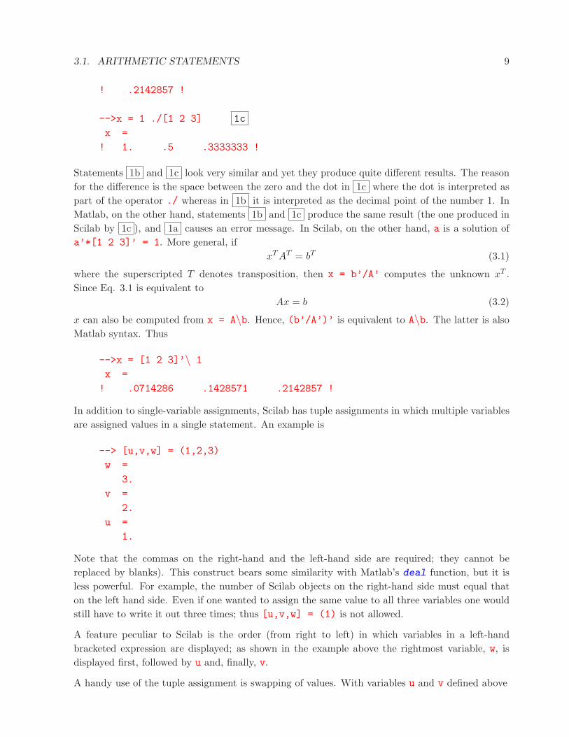
3.1. ARITHMETIC STATEMENTS 9
! .2142857 !
-->x = 1 ./[1 2 3] 1c
x =
! 1. .5 .3333333 !
Statements 1b and 1c look very similar and yet they produce quite different results. The reasonfor the difference is the space between the zero and the dot in 1c where the dot is interpreted aspart of the operator ./ whereas in 1b it is interpreted as the decimal point of the number 1. InMatlab, on the other hand, statements 1b and 1c produce the same result (the one produced inScilab by 1c ), and 1a causes an error message. In Scilab, on the other hand, a is a solution ofa’*[1 2 3]’ = 1. More general, if
xT AT = bT (3.1)
where the superscripted T denotes transposition, then x = b’/A’ computes the unknown xT .Since Eq. 3.1 is equivalent to
Ax = b (3.2)
x can also be computed from x = A\b. Hence, (b’/A’)’ is equivalent to A\b. The latter is alsoMatlab syntax. Thus
-->x = [1 2 3]’\ 1
x =
! .0714286 .1428571 .2142857 !
In addition to single-variable assignments, Scilab has tuple assignments in which multiple variablesare assigned values in a single statement. An example is
--> [u,v,w] = (1,2,3)
w =
3.
v =
2.
u =
1.
Note that the commas on the right-hand and the left-hand side are required; they cannot bereplaced by blanks). This construct bears some similarity with Matlab’s deal function, but it isless powerful. For example, the number of Scilab objects on the right-hand side must equal thaton the left hand side. Even if one wanted to assign the same value to all three variables one wouldstill have to write it out three times; thus [u,v,w] = (1) is not allowed.
A feature peculiar to Scilab is the order (from right to left) in which variables in a left-handbracketed expression are displayed; as shown in the example above the rightmost variable, w, isdisplayed first, followed by u and, finally, v.
A handy use of the tuple assignment is swapping of values. With variables u and v defined above
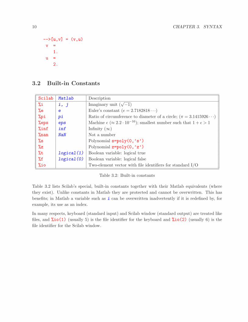
10 CHAPTER 3. SYNTAX
-->[u,v] = (v,u)
v =
1.
u =
2.
3.2 Built-in Constants
Scilab Matlab Description%i i, j Imaginary unit (
√−1)%e e Euler’s constant (e = 2.7182818 · · ·)%pi pi Ratio of circumference to diameter of a circle; (π = 3.1415926 · · ·)%eps eps Machine ε (≈ 2.2 · 10−16); smallest number such that 1 + ε > 1%inf inf Infinity (∞)%nan NaN Not a number%s Polynomial s=poly(0,’s’)%z Polynomial z=poly(0,’z’)%t logical(1) Boolean variable: logical true%f logical(0) Boolean variable: logical false%io Two-element vector with file identifiers for standard I/O
Table 3.2: Built-in constants
Table 3.2 lists Scilab’s special, built-in constants together with their Matlab equivalents (wherethey exist). Unlike constants in Matlab they are protected and cannot be overwritten. This hasbenefits; in Matlab a variable such as i can be overwritten inadvertently if it is redefined by, forexample, its use as an index.
In many respects, keyboard (standard input) and Scilab window (standard output) are treated likefiles, and %io(1) (usually 5) is the file identifier for the keyboard and %io(2) (usually 6) is thefile identifier for the Scilab window.

3.3. COMPARISON OPERATORS 11
3.3 Comparison Operators
Scilab uses the same comparison operators Matlab does, but with two choices for the “not equal”operator.
< less than> greater than
<= less than or equal to>= greater than or equal to== equal to
<> or ∼= not equal to
The result of a valid expression involving any of these operators — such as a > 0 — is a booleanvariable (%t or %f) or a matrix of boolean variables. These boolean variables are discussed later insection 4.4.
In Scilab the first four operators are only defined for real numbers; in Matlab complex numbers areallowed but only the real part is used for the comparison.
The last two operators compare objects. Examples are
-->[1 2 3] == 1 2a
ans =
! T F F !
-->[1 2 3] == [1 2] 2b
ans =
F
-->[1 2] == [’1’,’2’] 2c
ans =
F
In Matlab 2a produces the same result, 2b aborts with an error message, and 2c creates theboolean vector [0 0].
12 CHAPTER 3. SYNTAX
3.4 Flow Control
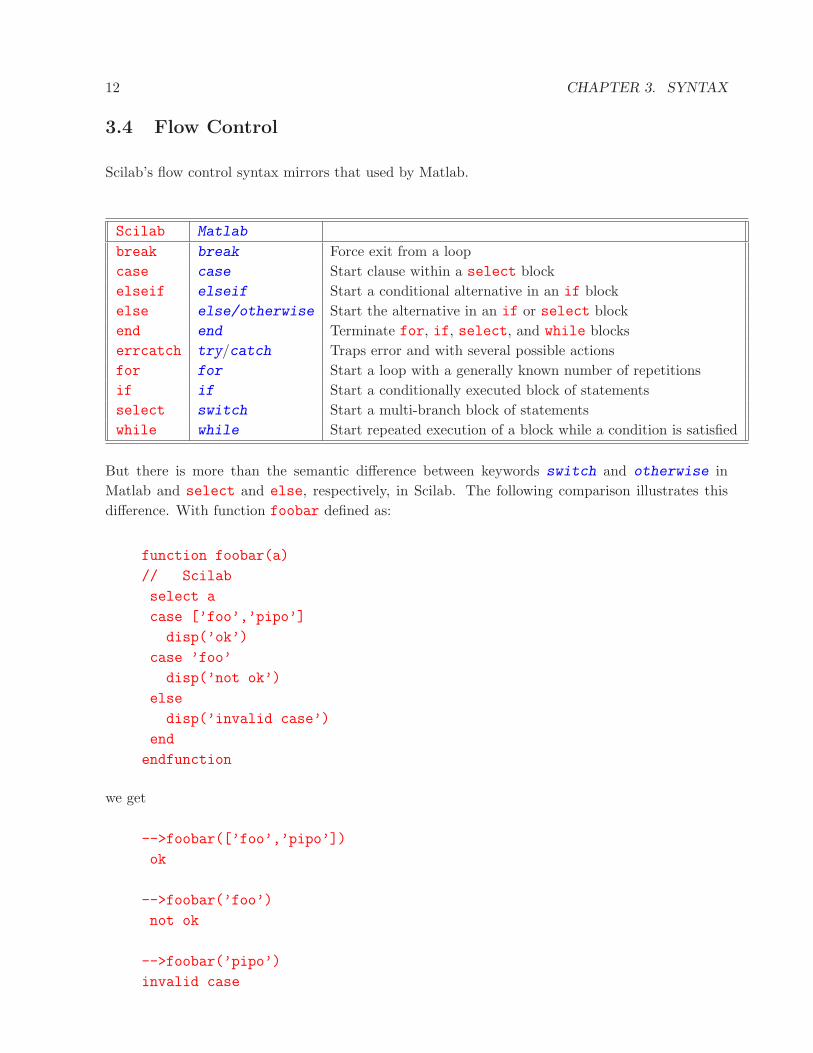
Scilab’s flow control syntax mirrors that used by Matlab.
Scilab Matlab
break break Force exit from a loopcase case Start clause within a select blockelseif elseif Start a conditional alternative in an if blockelse else/otherwise Start the alternative in an if or select blockend end Terminate for, if, select, and while blockserrcatch try/catch Traps error and with several possible actionsfor for Start a loop with a generally known number of repetitionsif if Start a conditionally executed block of statementsselect switch Start a multi-branch block of statementswhile while Start repeated execution of a block while a condition is satisfied
But there is more than the semantic difference between keywords switch and otherwise inMatlab and select and else, respectively, in Scilab. The following comparison illustrates thisdifference. With function foobar defined as:
function foobar(a)
// Scilab
select a
case [’foo’,’pipo’]
disp(’ok’)
case ’foo’
disp(’not ok’)
else
disp(’invalid case’)
end
endfunction
we get
-->foobar([’foo’,’pipo’])
ok
-->foobar(’foo’)
not ok
-->foobar(’pipo’)
invalid case

3.4. FLOW CONTROL 13
The variable a following the keyword select can be any Scilab data object.
The analogous Matlab function
function foobar(a)
% Matlab
switch a
case {’foo’,’pipo’}disp(’ok’)
case ’foo’
disp(’not ok’)
otherwise
disp(’invalid case’)
end
on the other hand, leads to
>>foobar({’foo’,’pipo’})??? SWITCH expression must result in a scalar or string constant.
>>foobar(’foo’)
ok
>>foobar(’pipo’)
ok
The variable a following the keyword switch can only be a scalar or string constant. On the otherhand, a case can represent more than one value of the variable. The strings ’foo’ and ’pipo’
satisfy the first case and so the second case is never reached.
In an if clause Scilab has the optional keywords then and do as in
-->if a >= 0 then a=sqrt(a); end
-->if a >= 0 do a=sqrt(a); end
but then and do can be replaced by a comma, a semicolon, or a <RETURN>. Hence, bothstatements are equivalent to
-->if a >= 0, a=sqrt(a); end
Likewise, the for loop can be written with the optional keyword do as in
for i = 1:n do a(i)=asin(2*%pi*i); end

14 CHAPTER 3. SYNTAX
and again do can be replaced by a comma, a semicolon, or a <RETURN>. The same is true forthe while clause.
Matlab uses the try/catch syntax to trap errors. Its functionality can be emulated by means thecombination of errcatch and iserror. This is illustrated in the following code fragment1. Forthe sake of clarity it is shown here the way it would look in a file.
errcatch(-1,’continue’,’nomessage’); // Start error trapping 3
a=1/0 4a
if iserror() // Check for error
disp(’A division by zero has occurred’)
errclear(-1)
end
a=1/0 4b
b=1
errclear(-1)
errcatch(-1) // Error trapping toggled off
a=1/0 4c
Statement 3 starts error trapping with the system error message suppressed. Statements 4a ,4b , and 4b represent errors. Execution of these statements produces the following result:
-->errcatch(-1,’continue’,’nomessage’); // Start error trapping 3
-->a=1/0 4a
-->if iserror() // Check for error
--> disp(’A division by zero has occurred’)
A division by zero has occurred
--> errclear(-1)
-->end
-->
-->a=1/0 4b
-->b=1
b =
1.
1errcatch is considered “fragile”, and thus this construct should be used only for debugging; for more robust
code the use of execstr(· · ·,’errcatch’) is preferable.

3.5. GENERAL FUNCTIONS 15
-->errclear(-1)
-->errcatch(-1) // Error trapping toggled off
-->a=1/0 4c
!--error 27
division by zero...
Clearly, the three identical “division by zero” errors are treated differently. The first one, 4a , istrapped and the user-supplied message is printed; the second, 4b , is trapped and ignored; thethird division by zero, 4c , occurs after error trapping has been turned off and creates the standardsystem error message.
Other commands can be considered as at least related to flow control. They include pause whichinterrupts execution similar to Scilab’s keyboard command, but with some important differencesexplained beginning on page 15.
Another function, halt, can be used to temporarily interrupt a program or script. Execution of afunction or script will stop upon encountering halt() and wait for a key press before continuing.
3.5 General Functions
Table 3.3 lists Scilab’s low-level functions and commands (commands are actually functions usedwith command-style syntax; see Section 5.1). Some, like date, are essentially the same as in Matlab,others have slightly different names (exists vs. exist), some may have the same name but maygive slightly different output (in Scilab length with a matrix argument returns the product ofthe number of rows and columns, in Matlab length returns the larger of the number of rows andcolumns), and many are quite different.
In this list of functions the command pause deserves special attention. It is equivalent to Matlab’skeyboard command in that it interrupts the flow of a script or function and returns control to thekeyboard. However, a Matlab function/script stays in the workspace of the function. In Scilab thepause command creates a new workspace. The prompt changes from, say, --> to -1-> where thenumber 1 indicates the workspace level. All variables of all lower workspace are available at thisnew workspace as long as they are not shadowed (a variable in a lower workspace is shadowed if avariable with the same name is defined in a higher workspace). This is an example:
-->a = 1, b = 2 // Variables in original workspace
a =
1.
b =
2.
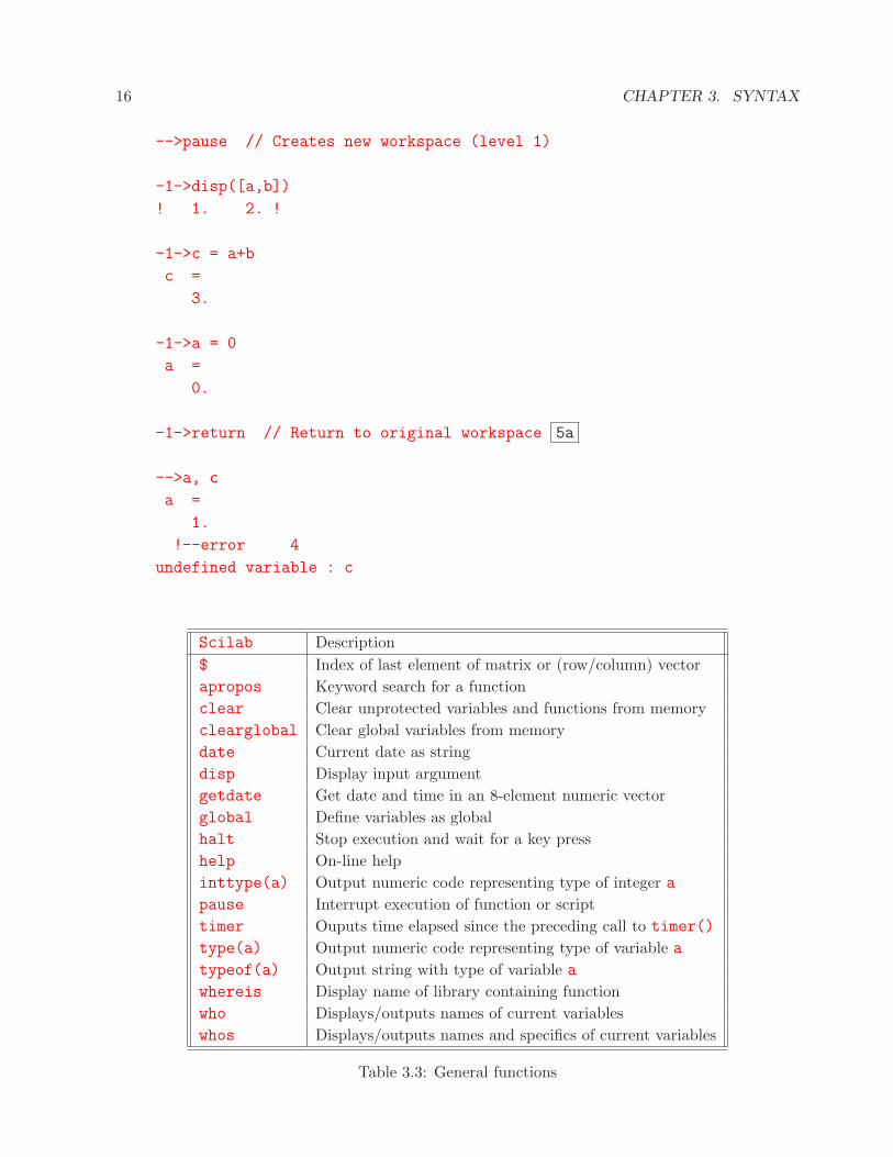
16 CHAPTER 3. SYNTAX
-->pause // Creates new workspace (level 1)
-1->disp([a,b])
! 1. 2. !
-1->c = a+b
c =
3.
-1->a = 0
a =
0.
-1->return // Return to original workspace 5a
-->a, c
a =
1.
!--error 4
undefined variable : c
Scilab Description$ Index of last element of matrix or (row/column) vectorapropos Keyword search for a functionclear Clear unprotected variables and functions from memoryclearglobal Clear global variables from memorydate Current date as stringdisp Display input argumentgetdate Get date and time in an 8-element numeric vectorglobal Define variables as globalhalt Stop execution and wait for a key presshelp On-line helpinttype(a) Output numeric code representing type of integer apause Interrupt execution of function or scripttimer Ouputs time elapsed since the preceding call to timer()
type(a) Output numeric code representing type of variable atypeof(a) Output string with type of variable awhereis Display name of library containing functionwho Displays/outputs names of current variableswhos Displays/outputs names and specifics of current variables
Table 3.3: General functions

3.5. GENERAL FUNCTIONS 17
The command pause creates a new workspace (the level of this workspace becomes part of theprompt); the display function disp shows that the variables a and b are available in this newworkspace, and the new variable c is computed correctly. However, upon returning to the originalworkspace we find that a still has the value 1 (in spite of being changed in the level-1 workspace)and that the variable c is not available anymore. This is not what we would have found withMatlab’s keyboard command.
In order to get these new values to the original workspace they have to be passed on by the returncommand. In Scilab the return command can have input and output arguments!
-->a = 1, b = 2
a =
1.
b =
2.
-->pause // Create new workspace (level 1)
-1->disp([a,b])
! 1. 2. !
-1->c = a+b
c =
3.
-1->a = 0
a =
0.
-1->[aa,c] = return(a,c) // Return to original workspace 5b
-->aa,c
aa =
0.
c =
3.
The above two code fragments are identical except for the return statements 5a and 5b . State-ment 5b returns variables a and c created in the level-1 workspace renaming a to aa. Withoutthis change, the existing variable a would have overwritten by the value of a created in the level-1workspace. A more complicated use of the return function is illustrated in statement 29 on page82.

18 CHAPTER 3. SYNTAX
The command resume is equivalent to the return command (we could have used resume insteadof return in the two examples above).
Unlike its Matlab counterpart, the display function disp, which has already been used above,allows more than one input parameter:
-->disp(123,’The result is:’)
The result is:
123.
It shows the same behavior noted previously: the input arguments are printed to the screen begin-ning with the last.

Chapter 4
Variable Types
The only two variable types a casual user is likely to define and use are numeric variables andstrings; but Scilab has many more data types — in fact, it has more than Matlab. Hence, it isimportant to be able to identify them. Unlike Matlab, which uses specific functions with booleanoutput for each variable type (e. g. iscell, ischar, isnumeric, issparse, isstruct), Scilabuses essentially two functions, type and typeof: the former has numeric output the other outputsa character string. The following table lists variable types and the output of type and typeof.The last column of this table, with heading “Op-type”, defines the abbreviation used to specify theoperand type for operator overloading (see Section 7.3).
Type of variable type typeof Op-typereal or complex constant matrix 1 ’constant’ spolynomial matrix 2 ’polynomial’ pboolean matrix 4 ’boolean’ bsparse matrix 5 ’sparse’ spsparse boolean matrix 6 ’boolean sparse’ spbMatlab sparse matrix 7 ? mspmatrix of integers stored in 1, 2, or 4 bytes 8 Depends on type of integer imatrix of character strings 10 ’string’ cfunction (un-compiled) 11 ’function’ mfunction (compiled) 13 ’function’ mcfunction library 14 ’library’ flist 15 ’list’ ltyped list (tlist) 16 Depends on type of list tlmatrix-like typed list (mlist) 17 Depends on type of list mlpointer 128 ? ptrindex vector with implicit size 129 ’size implicit’ ip
Table 4.1: Variable types
19
20 CHAPTER 4. VARIABLE TYPES
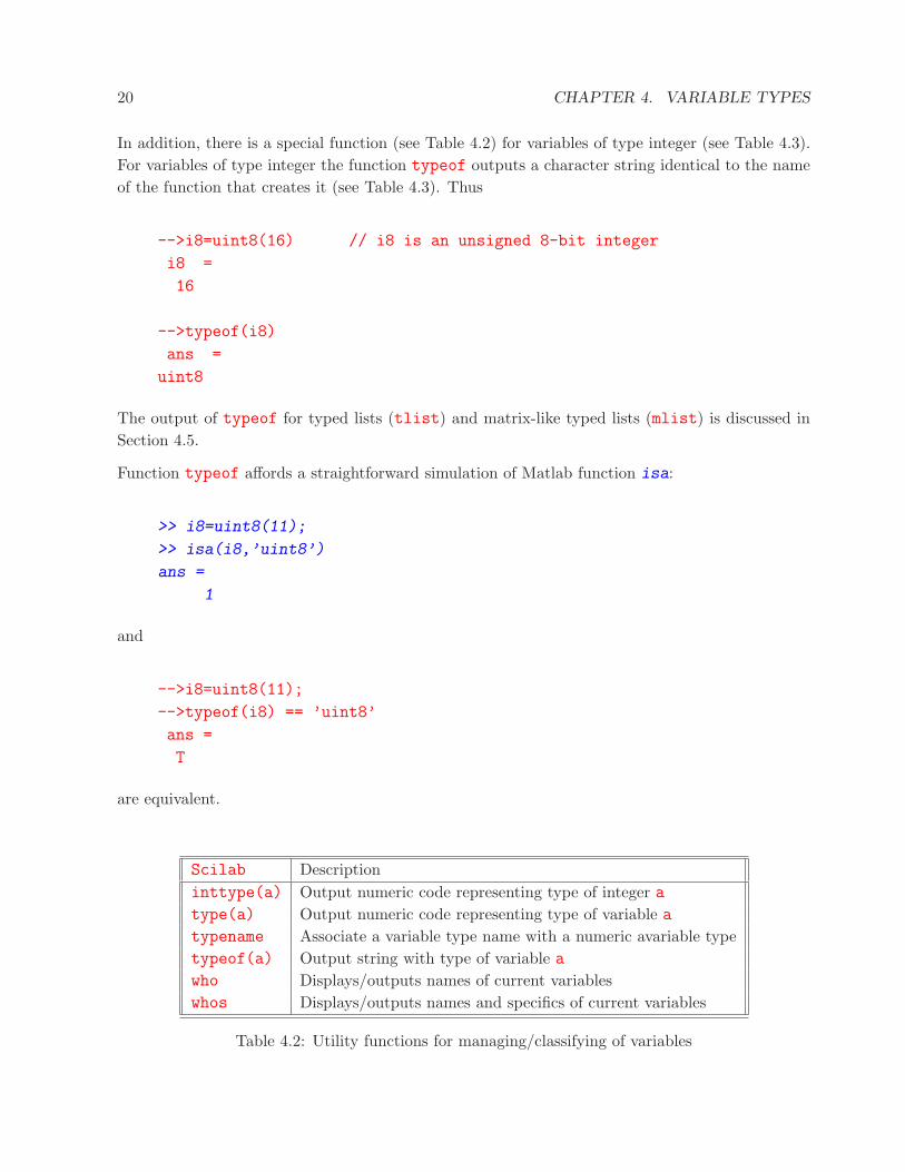
In addition, there is a special function (see Table 4.2) for variables of type integer (see Table 4.3).For variables of type integer the function typeof outputs a character string identical to the nameof the function that creates it (see Table 4.3). Thus
-->i8=uint8(16) // i8 is an unsigned 8-bit integer
i8 =
16
-->typeof(i8)
ans =
uint8
The output of typeof for typed lists (tlist) and matrix-like typed lists (mlist) is discussed inSection 4.5.
Function typeof affords a straightforward simulation of Matlab function isa:
>> i8=uint8(11);
>> isa(i8,’uint8’)
ans =
1
and
-->i8=uint8(11);
-->typeof(i8) == ’uint8’
ans =
T
are equivalent.
Scilab Descriptioninttype(a) Output numeric code representing type of integer atype(a) Output numeric code representing type of variable atypename Associate a variable type name with a numeric avariable typetypeof(a) Output string with type of variable awho Displays/outputs names of current variableswhos Displays/outputs names and specifics of current variables
Table 4.2: Utility functions for managing/classifying of variables

4.1. NUMERIC VARIABLES — SCALARS AND MATRICES 21
4.1 Numeric Variables — Scalars and Matrices
Scilab knows matrices. This term includes scalars and vectors. Scalars and the elements of vectorsand matrices can be real or complex. The statements
-->a = 1.2;
-->b = 1.0e3;
-->cx = a+%i*b
cx =
1.2 + 1000.i
define three 1 × 1 matrices, i.e. scalars. There is no function like complex in Scilab. Defining acomplex number, such as cx above, is done via an arithmetic statement.
Vectors and matrices can be entered and accessed in much the same way as in Matlab.
-->mat=[ 1 2 3; 4 5 6]
mat =
! 1. 2. 3. !
! 4. 5. 6. !
-->mat2=[mat;mat+6]
mat2 =
! 1. 2. 3. !
! 4. 5. 6. !
! 7. 8. 9. !
! 10. 11. 12. !
-->mat(2,3)
ans =
6.
-->mat(2,:)
ans =
! 4. 5. 6. !
-->mat($,$)
ans =
6.
-->mat($)
ans = 6.

22 CHAPTER 4. VARIABLE TYPES
There is a difference in the way the last element of a vector or matrix is accessed. Scilab usesthe $ sign as indicator of the last element whereas Matlab uses end. The $ represents, in fact, asomewhat more powerful concept and can be used to create an implied-size vector, a new variableof type ’size implicit’.
-->index=2:$
index =
2:1:$
-->type(index)
ans =
129.
-->typeof(index)
ans =
size implicit
-->mat2(2,index)
ans =
! 5. 6. !
There is no equivalent in Matlab for this kind of addressing of matrix elements.
By default, Scilab variables are double-precision floating point numbers. However, like Matlab,Scilab also knows integers. Conversion functions are shown in Table 4.3. Function iconvert,which takes two input arguments, does essentially what the seven other conversion functions listedin this table do.
Scilab Descriptiondouble Convert integer array of any type/length to floating point arrayiconvert Convert numeric array to any integer or floating point formatint8(a) Convert a to an 8-bit signed integerint16(a) Convert a to a 16-bit signed integerint32(a) Convert a to a 32-bit signed integeruint8(a) Convert a to an 8-bit unsigned integeruint16(a) Convert a to a 16-bit unsigned integeruint32(a) Convert a to a 32-bit unsigned integer
Table 4.3: Integer conversion functions
Matlab allows no mathematical operations for such integers. Scilab is more lenient and lets theuser worry about wrap-around and possibly other problems.

4.1. NUMERIC VARIABLES — SCALARS AND MATRICES 23
-->u = int8(100), v = int8(2)
u =
100
v =
2
-->u*v
ans =
-56
The result is wrapped (200-256). Unsigned integers give an analogous result.
-->x = uint8(100), y = uint8(2), z= uint8(3)
idxuint8
x =
100
y =
2
z =
3
-->x*y
ans =
200
-->x*z
ans = 44
Again, the last result is wrapped (300-256). Operations between integers of different type are notallowed, but those with standard (double precision) floating point numbers are, and the result is afloating point number.
-->typeof(z)
ans =
uint8
-->typeof(2*z)
ans =
constant
The variable z, defined in the previous example, is an unsigned one-byte integer. Multiply it by 2and the result is a regular floating point number for which typeof returns the value constant.

24 CHAPTER 4. VARIABLE TYPES
4.2 Special Matrices
Like Matlab, Scilab has a number of functions that create “standard” matrices. Many of them havethe same or a very similar names. The arguments or the output may be slightly different.
The empty matrix [] in Scilab behaves slightly different than the corresponding [ ] in Matlab; inScilab, for example,
-->a = []+3 6a
a =
3.
whereas in Matlab
>>a = []+3 6b
a =
[].
Scilab Description[] Empty matrixcompanion Companion matrixdiag Create diagonal matrix or extract diagonal from matrixeye Identity matrix (or its generalization)grand Create random numbers drawn from various distributionsones Matrix of onesrand Matrix of random numbers with uniform or normal distributionsylm Sylvester matrix (input two polynomials, output numeric)testmatrix Test matrices: magic square, Franck matrix, inverse of Hilbert matrixtoeplitz Toeplitz matrixzeros Matrix of zeros
Table 4.4: Special matrices
While 6a is the default result, Scilab’s behavior in this situation can be changed by invokingMatlab-mode.
-->mtlb mode(%t)
-->a = []+3 6c
a =
[]
4.3. CHARACTER STRING VARIABLES 25
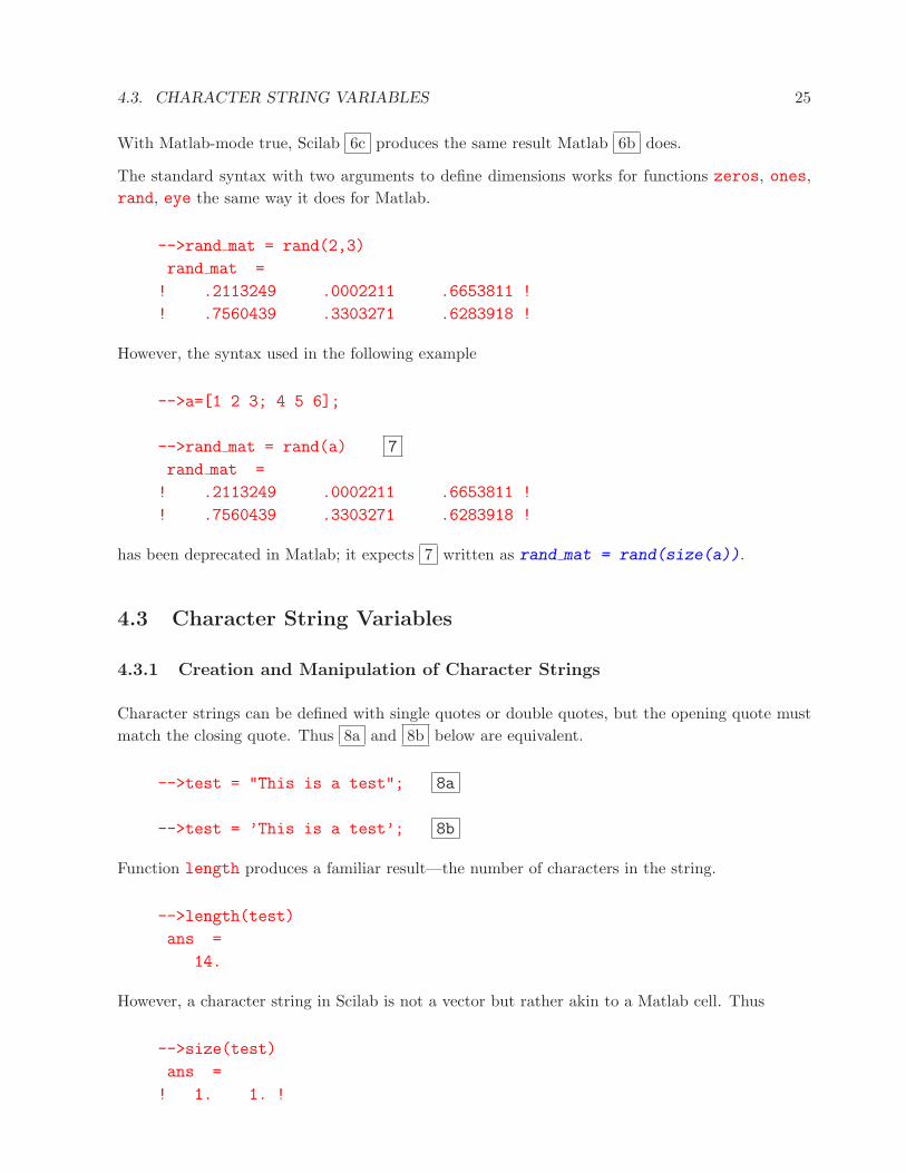
With Matlab-mode true, Scilab 6c produces the same result Matlab 6b does.
The standard syntax with two arguments to define dimensions works for functions zeros, ones,rand, eye the same way it does for Matlab.
-->rand mat = rand(2,3)
rand mat =
! .2113249 .0002211 .6653811 !
! .7560439 .3303271 .6283918 !
However, the syntax used in the following example
-->a=[1 2 3; 4 5 6];
-->rand mat = rand(a) 7
rand mat =
! .2113249 .0002211 .6653811 !
! .7560439 .3303271 .6283918 !
has been deprecated in Matlab; it expects 7 written as rand mat = rand(size(a)).
4.3 Character String Variables
4.3.1 Creation and Manipulation of Character Strings
Character strings can be defined with single quotes or double quotes, but the opening quote mustmatch the closing quote. Thus 8a and 8b below are equivalent.
-->test = "This is a test"; 8a
-->test = ’This is a test’; 8b
Function length produces a familiar result—the number of characters in the string.
-->length(test)
ans =
14.
However, a character string in Scilab is not a vector but rather akin to a Matlab cell. Thus
-->size(test)
ans =
! 1. 1. !
26 CHAPTER 4. VARIABLE TYPES
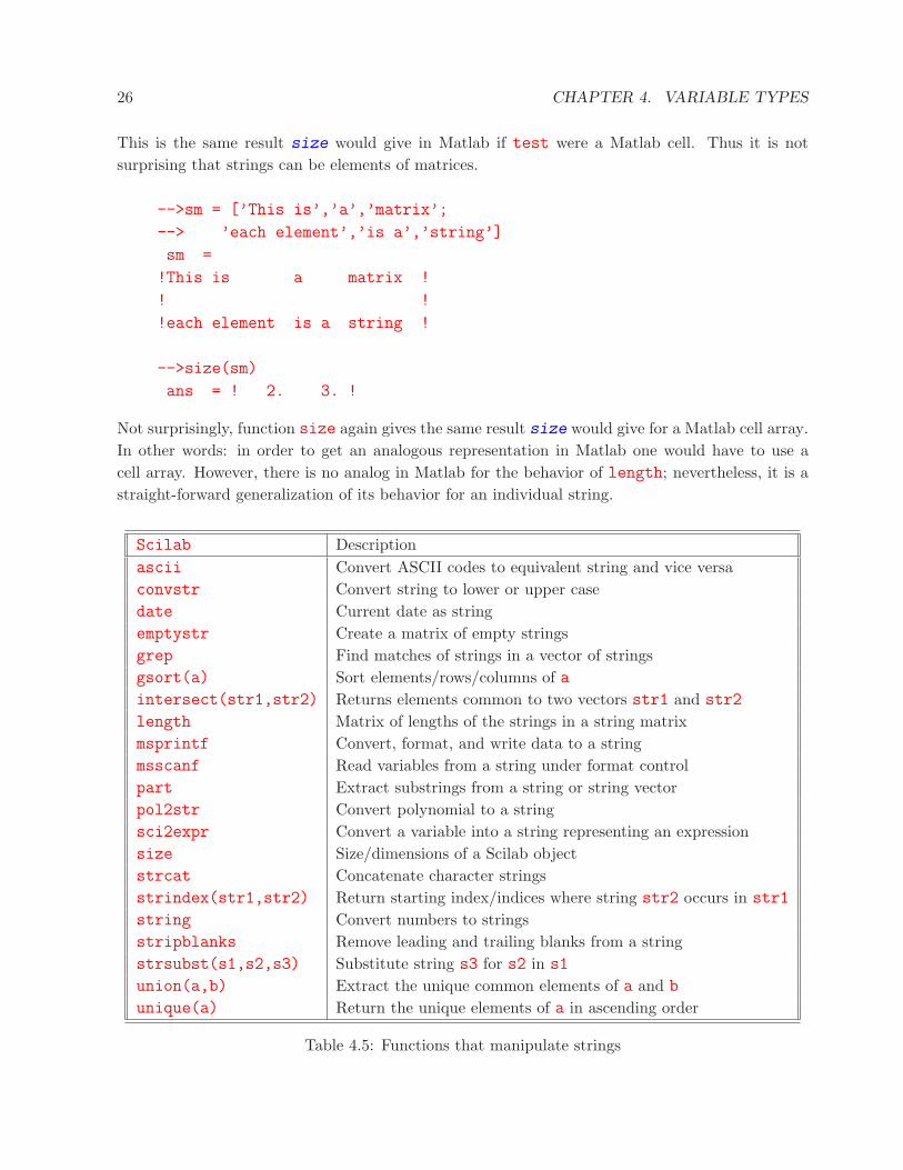
This is the same result size would give in Matlab if test were a Matlab cell. Thus it is notsurprising that strings can be elements of matrices.
-->sm = [’This is’,’a’,’matrix’;
--> ’each element’,’is a’,’string’]
sm =
!This is a matrix !
! !
!each element is a string !
-->size(sm)
ans = ! 2. 3. !
Not surprisingly, function size again gives the same result size would give for a Matlab cell array.In other words: in order to get an analogous representation in Matlab one would have to use acell array. However, there is no analog in Matlab for the behavior of length; nevertheless, it is astraight-forward generalization of its behavior for an individual string.
Scilab Descriptionascii Convert ASCII codes to equivalent string and vice versaconvstr Convert string to lower or upper casedate Current date as stringemptystr Create a matrix of empty stringsgrep Find matches of strings in a vector of stringsgsort(a) Sort elements/rows/columns of aintersect(str1,str2) Returns elements common to two vectors str1 and str2
length Matrix of lengths of the strings in a string matrixmsprintf Convert, format, and write data to a stringmsscanf Read variables from a string under format controlpart Extract substrings from a string or string vectorpol2str Convert polynomial to a stringsci2expr Convert a variable into a string representing an expressionsize Size/dimensions of a Scilab objectstrcat Concatenate character stringsstrindex(str1,str2) Return starting index/indices where string str2 occurs in str1
string Convert numbers to stringsstripblanks Remove leading and trailing blanks from a stringstrsubst(s1,s2,s3) Substitute string s3 for s2 in s1
union(a,b) Extract the unique common elements of a and b
unique(a) Return the unique elements of a in ascending order
Table 4.5: Functions that manipulate strings

4.3. CHARACTER STRING VARIABLES 27
-->length(sm)
ans =
! 7. 1. 6. !
! 12. 4. 6. !
The output of length is a matrix with the same dimension as sm; each matrix entry is the numberof characters of the corresponding entry of sm. For many purposes this output is so useful that onemisses it in Matlab.
A handy function for many string manipulations is ascii which converts character strings intotheir ASCII equivalent (e.g. ’A’ to 65, ’a’ to 97) and vice versa. In fact, beginning with Scilab2.6, it even supports the 8-bit ASCII standard (including the Euro which recently replaced the“international currency symbol”). Function ascii does in Scilab what the pair char and double
does in Matlab.
Below is an example where ascii is used to emulate Matlab function isletter.
function bool=isletter(str)
// Function creates a boolean vector bool the length of which is
// equal to the number of characters in string str.
// An element of bool is true if the corresponding character in
// str is a letter and false if it is not not.
// INPUT
// str character string
// OUTPUT
// bool boolean vector
temp = ascii(str);
bool = (temp >= 65 & temp <= 90) | (temp >= 97 & temp <= 122);
endfunction
With this function
-->isletter(’abc123 END.’)
ans =
! T T T F F F F T T T F !
Strings can be concatenated by means of the + sign
-->s1 = ’Example’;
-->s2 = ’of ’;
-->s3 = ’concatenation’;
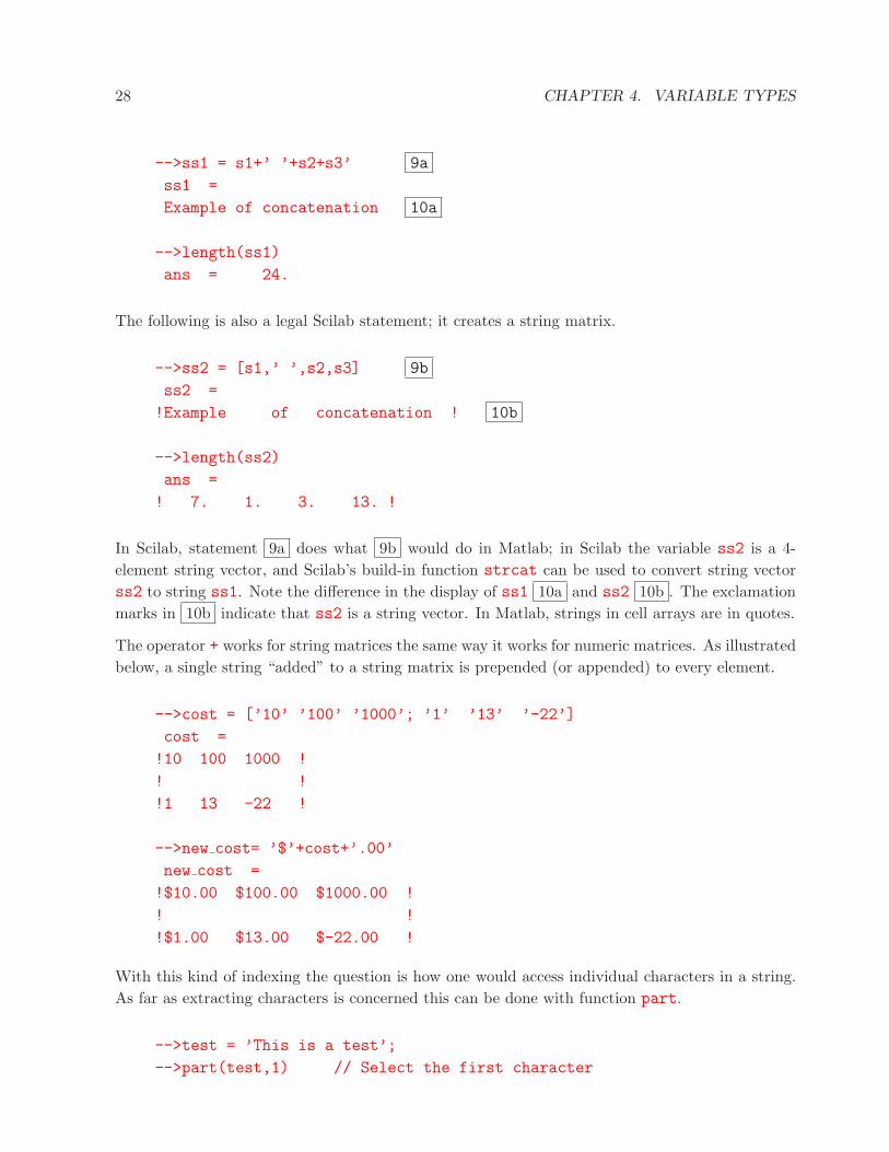
28 CHAPTER 4. VARIABLE TYPES
-->ss1 = s1+’ ’+s2+s3’ 9a
ss1 =
Example of concatenation 10a
-->length(ss1)
ans = 24.
The following is also a legal Scilab statement; it creates a string matrix.
-->ss2 = [s1,’ ’,s2,s3] 9b
ss2 =
!Example of concatenation ! 10b
-->length(ss2)
ans =
! 7. 1. 3. 13. !
In Scilab, statement 9a does what 9b would do in Matlab; in Scilab the variable ss2 is a 4-element string vector, and Scilab’s build-in function strcat can be used to convert string vectorss2 to string ss1. Note the difference in the display of ss1 10a and ss2 10b . The exclamationmarks in 10b indicate that ss2 is a string vector. In Matlab, strings in cell arrays are in quotes.
The operator + works for string matrices the same way it works for numeric matrices. As illustratedbelow, a single string “added” to a string matrix is prepended (or appended) to every element.
-->cost = [’10’ ’100’ ’1000’; ’1’ ’13’ ’-22’]
cost =
!10 100 1000 !
! !
!1 13 -22 !
-->new cost= ’$’+cost+’.00’
new cost =
!$10.00 $100.00 $1000.00 !
! !
!$1.00 $13.00 $-22.00 !
With this kind of indexing the question is how one would access individual characters in a string.As far as extracting characters is concerned this can be done with function part.
-->test = ’This is a test’;
-->part(test,1) // Select the first character
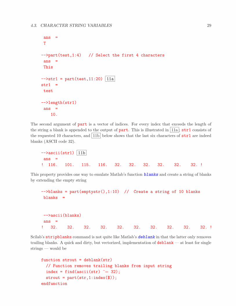
4.3. CHARACTER STRING VARIABLES 29
ans =
T
-->part(test,1:4) // Select the first 4 characters
ans =
This
-->str1 = part(test,11:20) 11a
str1 =
test
-->length(str1)
ans =
10.
The second argument of part is a vector of indices. For every index that exceeds the length ofthe string a blank is appended to the output of part. This is illustrated in 11a ; str1 consists ofthe requested 10 characters, and 11b below shows that the last six characters of str1 are indeedblanks (ASCII code 32).
-->ascii(str1) 11b
ans =
! 116. 101. 115. 116. 32. 32. 32. 32. 32. 32. !
This property provides one way to emulate Matlab’s function blanks and create a string of blanksby extending the empty string
-->blanks = part(emptystr(),1:10) // Create a string of 10 blanks
blanks =
-->ascii(blanks)
ans =
! 32. 32. 32. 32. 32. 32. 32. 32. 32. 32. !
Scilab’s stripblanks command is not quite like Matlab’s deblank in that the latter only removestrailing blanks. A quick and dirty, but vectorized, implementation of deblank — at least for singlestrings — would be
function strout = deblank(str)
// Function removes trailing blanks from input string
index = find(ascii(str) ˜= 32);
strout = part(str,1:index($));
endfunction
30 CHAPTER 4. VARIABLE TYPES
which again uses functions part and ascii. This example again illustrates the use of $ to denotethe last element of a vector — analogous to the use of end in Matlab as the last index. The simplemodification required in the last statement to remove leading blanks (or leading and trailing blanks)is obvious.
It is worth reviewing a few more of the functions shown in Table 4.5.
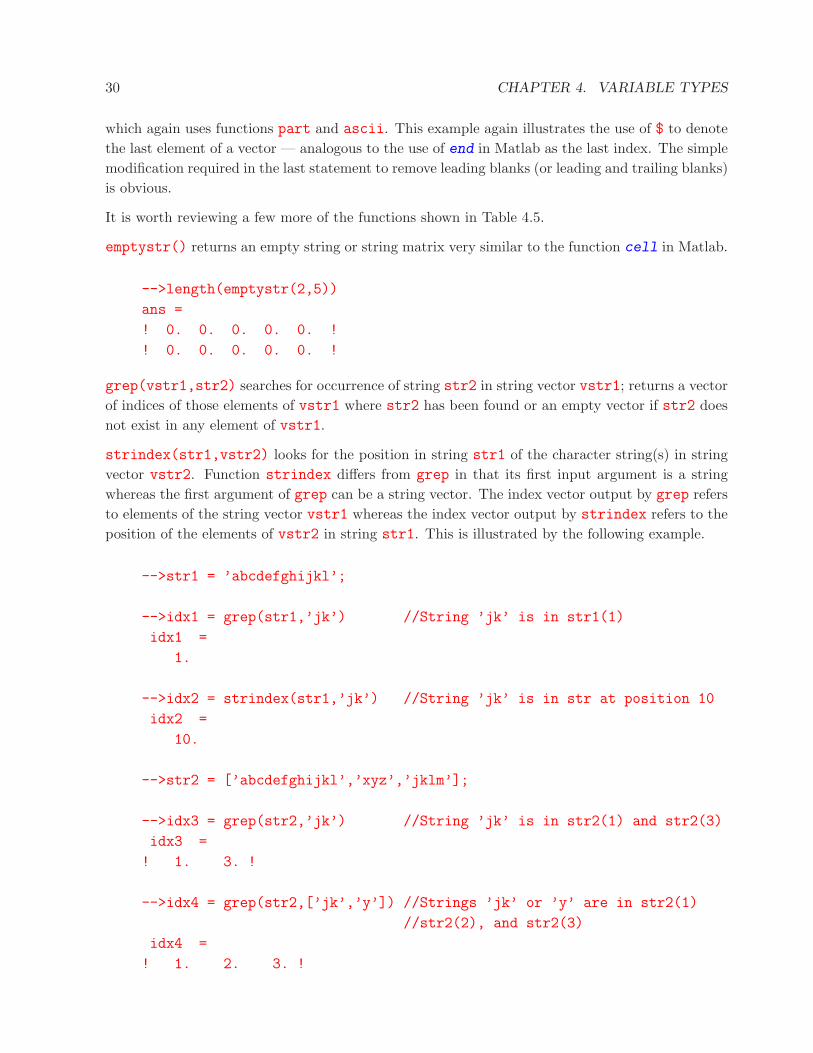
emptystr() returns an empty string or string matrix very similar to the function cell in Matlab.
-->length(emptystr(2,5))
ans =
! 0. 0. 0. 0. 0. !
! 0. 0. 0. 0. 0. !
grep(vstr1,str2) searches for occurrence of string str2 in string vector vstr1; returns a vectorof indices of those elements of vstr1 where str2 has been found or an empty vector if str2 doesnot exist in any element of vstr1.
strindex(str1,vstr2) looks for the position in string str1 of the character string(s) in stringvector vstr2. Function strindex differs from grep in that its first input argument is a stringwhereas the first argument of grep can be a string vector. The index vector output by grep refersto elements of the string vector vstr1 whereas the index vector output by strindex refers to theposition of the elements of vstr2 in string str1. This is illustrated by the following example.
-->str1 = ’abcdefghijkl’;
-->idx1 = grep(str1,’jk’) //String ’jk’ is in str1(1)
idx1 =
1.
-->idx2 = strindex(str1,’jk’) //String ’jk’ is in str at position 10
idx2 =
10.
-->str2 = [’abcdefghijkl’,’xyz’,’jklm’];
-->idx3 = grep(str2,’jk’) //String ’jk’ is in str2(1) and str2(3)
idx3 =
! 1. 3. !
-->idx4 = grep(str2,[’jk’,’y’]) //Strings ’jk’ or ’y’ are in str2(1)
//str2(2), and str2(3)
idx4 =
! 1. 2. 3. !

4.3. CHARACTER STRING VARIABLES 31
This means that grep with some additional checking can be used to emulate the Matlab functionismember for string arguments (see page 39).
Like its Matlab equivalent the function msscanf can be use to extract substrings separated byspaces and numbers from a string.
-->str=’ Weight: 2.5 kg’;
-->[a,b,c] = msscanf(str,’%s%f%s’)
c =
kg
b =
2.5
a =
Weight:
-->typeof(a)
ans =
string
-->typeof(b)
ans =
constant
The format types available are %s for strings, %e, %f, %g for floating-point numbers, %d, %i fordecimal integers, %u for unsigned integers, %o for octal numbers, %x for hexadecimal numbers,and %c for a characters (white spaces are not skipped). For more details see the help file forscanf conversion.
In the context of the next subsection the function sci2exp may come in handy. It converts avariable into a string representing a Scilab expression. An example is
-->a=[1 2 3 4]’
a =
! 1. !
! 2. !
! 3. !
! 4. !
-->stringa = sci2exp(a)
stringa =
[1;2;3;4]
32 CHAPTER 4. VARIABLE TYPES
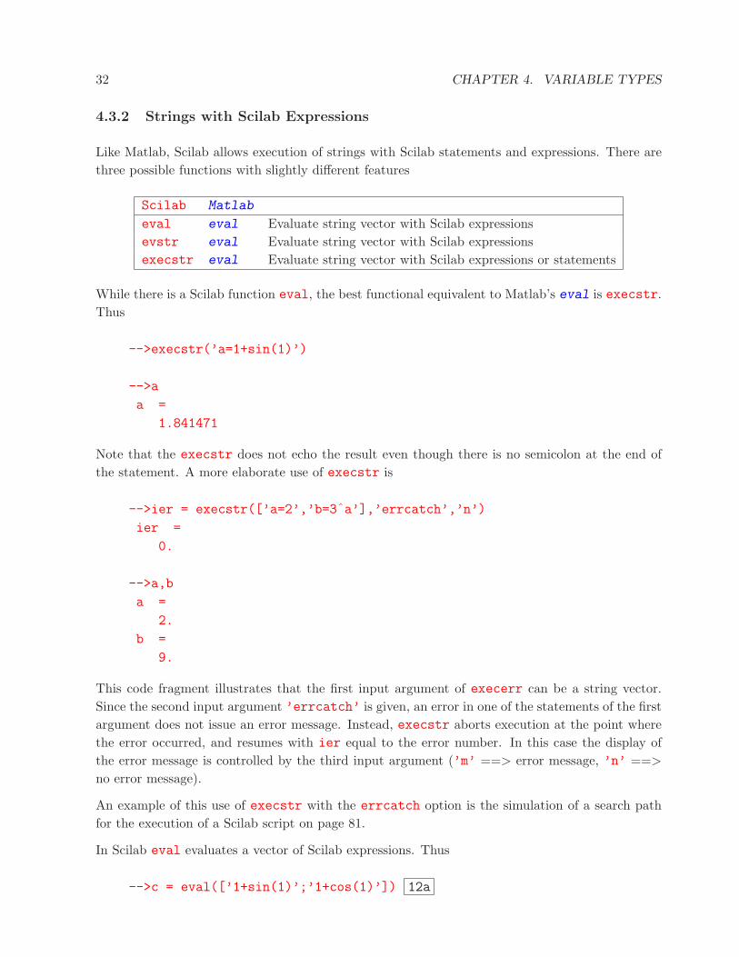
4.3.2 Strings with Scilab Expressions
Like Matlab, Scilab allows execution of strings with Scilab statements and expressions. There arethree possible functions with slightly different features
Scilab Matlab
eval eval Evaluate string vector with Scilab expressionsevstr eval Evaluate string vector with Scilab expressionsexecstr eval Evaluate string vector with Scilab expressions or statements
While there is a Scilab function eval, the best functional equivalent to Matlab’s eval is execstr.Thus
-->execstr(’a=1+sin(1)’)
-->a
a =
1.841471
Note that the execstr does not echo the result even though there is no semicolon at the end ofthe statement. A more elaborate use of execstr is
-->ier = execstr([’a=2’,’b=3ˆa’],’errcatch’,’n’)
ier =
0.
-->a,b
a =
2.
b =
9.
This code fragment illustrates that the first input argument of execerr can be a string vector.Since the second input argument ’errcatch’ is given, an error in one of the statements of the firstargument does not issue an error message. Instead, execstr aborts execution at the point wherethe error occurred, and resumes with ier equal to the error number. In this case the display ofthe error message is controlled by the third input argument (’m’ ==> error message, ’n’ ==>
no error message).
An example of this use of execstr with the errcatch option is the simulation of a search pathfor the execution of a Scilab script on page 81.
In Scilab eval evaluates a vector of Scilab expressions. Thus
-->c = eval([’1+sin(1)’;’1+cos(1)’]) 12a
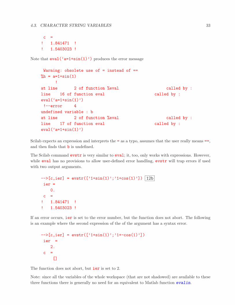
4.3. CHARACTER STRING VARIABLES 33
c =
! 1.841471 !
! 1.5403023 !
Note that eval(’a=1+sin(1)’) produces the error message
Warning: obsolete use of = instead of ==
%h = a=1+sin(1)
!
at line 2 of function %eval called by :
line 16 of function eval called by :
eval(’a=1+sin(1)’)
!--error 4
undefined variable : b
at line 2 of function %eval called by :
line 17 of function eval called by :
eval(’a=1+sin(1)’)
Scilab expects an expression and interprets the = as a typo, assumes that the user really means ==,and then finds that b is undefined.
The Scilab command evstr is very similar to eval; it, too, only works with expressions. However,while eval has no provisions to allow user-defined error handling, evstr will trap errors if usedwith two output arguments.
-->[c,ier] = evstr([’1+sin(1)’;’1+cos(1)’]) 12b
ier =
0.
c =
! 1.841471 !
! 1.5403023 !
If an error occurs, ier is set to the error number, but the function does not abort. The followingis an example where the second expression of the of the argument has a syntax error.
-->[c,ier] = evstr([’1+sin(1)’;’1+-cos(1)’])
ier =
2.
c =
[]
The function does not abort, but ier is set to 2.
Note: since all the variables of the whole workspace (that are not shadowed) are available to thesethree functions there is generally no need for an equivalent to Matlab function evalin.

34 CHAPTER 4. VARIABLE TYPES
4.3.3 Symbolic String Manipulation
Scilab has several function that treat strings as variables and perform symbolic operations. Anexamples is trianfml which converts a symbolic matrix to upper triangular form.
-->mat = [’a’,’b+c’,’d’;’-b*a’,’0’,’a+b’;’b’,’1’,’-1’]
mat =
!a b+c d !
! !
!-b*a 0 a+b !
! !
!b 1 -1 !
-->tri = trianfml(mat)
tri =
!b 1 -1 !
! !
!0 b*a b*(a+b)-b*a !
! !
!0 0 b*a*(b*d+a)-(b*(b+c)-a)*(b*(a+b)-b*a) !
A symbolic matrix can be evaluated by means of the function evstr discussed above.
-->a = 1,b = -1,c = 2,d = 0
a =
1.
b =
- 1.
c =
2.
d =
0.
-->nummat = evstr(tri)
nummat =
! - 1. 1. - 1. !
! 0. - 1. 1. !
! 0. 0. 1. !
There are several functions such as solve and trisolve that operate on symbolic matrices andaddf, subf, mulf, ldivf, and rdivf that operate on symbols representing scalars. What exactlythey do can be found by looking at their help files.

4.4. BOOLEAN VARIABLES 35
4.4 Boolean Variables
Boolean variables are represented by %t (true) and %f (false). Since Scilab’s main initialization fileequates the corresponding upper-case and lower-case variables they can also be used with capitalletters (%T, %F). This is different from Matlab where boolean variables, while intrinsically differentfrom arithmetic numbers, are represented by 1 and 0. This analogy is illustrated in the followingtable which shows a line-by-line comparison of corresponding Scilab and Matlab statements.
Scilab Matlab-->n = [1 1] >> n = [1 1]
n = n =
! 1. 1. ! 1 1
-->b = [%t,%t] >> b = logical([1,1])
b = b =
! T T ! 1 1
-->a = [1 2] >> a = [1 2]
a = a =
! 1. 2. ! 1 2
-->a(n) >> a(n)
ans = ans =
! 1. 1. ! 1 1
-->a(b) >> a(b)
ans = ans =
! 1. 2. ! 1 2
When displayed on the screen in Matlab, vectors n and b look exactly the same. Nevertheless, theyare different
>> islogical(n)
0
>> islogical(b)
1
and, when used as indices for the vector a, they produce different results. But, fortunately, theseresults agree with those obtained with Scilab.
There are three operators, well known from Matlab, that operate on boolean variables.

36 CHAPTER 4. VARIABLE TYPES
& Logical AND˜ Logical NOT| Logical OR
In the proper context, both Scilab and Matlab treat numeric variables like logical variables; anyreal numeric variable 6= 0 is interpreted as true and 0 is interpreted as false. Thus
-->if -1.34
--> a=1;
-->else
--> a=2;
-->end
-->a
a =
1.
Interestingly, Scilab itself is not very consistent regarding the use of boolean variables . The twofunctions exists and isdef do the same thing: they check if a variable exists. However, isdefoutputs T if the variable exists and F otherwise, whereas exists outputs 1 and 0, respectively.In this sense the function bool2s can be considered as having boolean output. If a is a numericmatrix, then b = bool2s(a) creates a matrix b where all non-zero entries of a are 1. If a isboolean then b is 1 where a is %t and 0 where a is %f. The same result — even without anexecution-time penalty — can be achieved by adding 0 to the boolean matrix a.
Since there is no Scilab function analogous to zeros or ones a similar trick must be used to createa boolean matrix or vector.
-->false = ˜ones(1,10)false =
! F F F F F F F F F F !
-->true = ˜˜ones(1,10)true =
! T T T T T T T T T T !
One could, in principle, define true as true=˜zeros(1,10), i. e. without the double negation,but in Scilab-2.6 function zeros is much slower than functions ones. This is expected to changein Scilab-2.7.
In Matlab all this would work as well but logical(ones(n,m)) is faster.
Like in Matlab, boolean variables can be used in arithmetic expressions where they act as if theywere 1 and 0, respectively.
-->5*%t

4.4. BOOLEAN VARIABLES 37
ans =
5.
-->3*%f
ans =
0.
Table 4.6 lists a number of functions that output or use boolean variables.
Functions and and or are functional equivalents of Matlab’s functions all and any, respectively.1
Function and(a) returns the boolean variable %t if all entries of a are %t (for a boolean matrix)or non-zero (for a numeric matrix).
a =
! 0. 1. !
! 2. 3. !
-->and(a)
ans =
F
-->and(a,’r’) 13
ans =
! F T !
In the example above a has a zero entry in the upper left corner; hence, the answer is false. Withthe optional second argument ’r’ (line 13 ), and analyzes the columns of a and outputs a rowvector. The first column contains a zero; hence the first element of the output vector is f. Matlab’sall would output an analogous logical vector.
Function or(a) returns the boolean variable %t if at least one entry of a is %t (for a booleanmatrix) or non-zero (for a numeric matrix). Hence, for the same matrix a
-->or(a)
ans =
T
-->or(a,’c’)
ans =
! T !
! T !
1See also the discussion of max, min, etc. on page 56
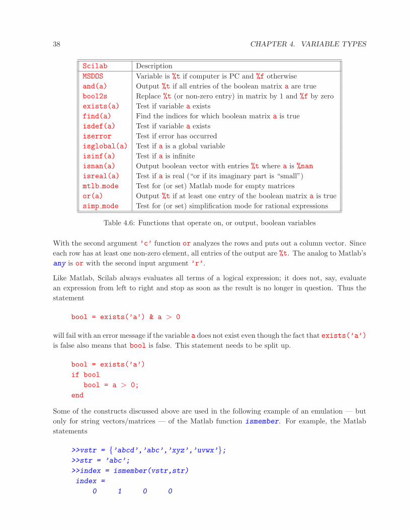
38 CHAPTER 4. VARIABLE TYPES
Scilab DescriptionMSDOS Variable is %t if computer is PC and %f otherwiseand(a) Output %t if all entries of the boolean matrix a are truebool2s Replace %t (or non-zero entry) in matrix by 1 and %f by zeroexists(a) Test if variable a existsfind(a) Find the indices for which boolean matrix a is trueisdef(a) Test if variable a existsiserror Test if error has occurredisglobal(a) Test if a is a global variableisinf(a) Test if a is infiniteisnan(a) Output boolean vector with entries %t where a is %nanisreal(a) Test if a is real (“or if its imaginary part is “small”)mtlb mode Test for (or set) Matlab mode for empty matricesor(a) Output %t if at least one entry of the boolean matrix a is truesimp mode Test for (or set) simplification mode for rational expressions
Table 4.6: Functions that operate on, or output, boolean variables
With the second argument ’c’ function or analyzes the rows and puts out a column vector. Sinceeach row has at least one non-zero element, all entries of the output are %t. The analog to Matlab’sany is or with the second input argument ’r’.
Like Matlab, Scilab always evaluates all terms of a logical expression; it does not, say, evaluatean expression from left to right and stop as soon as the result is no longer in question. Thus thestatement
bool = exists(’a’) & a > 0
will fail with an error message if the variable a does not exist even though the fact that exists(’a’)is false also means that bool is false. This statement needs to be split up.
bool = exists(’a’)
if bool
bool = a > 0;
end
Some of the constructs discussed above are used in the following example of an emulation — butonly for string vectors/matrices — of the Matlab function ismember. For example, the Matlabstatements
>>vstr = {’abcd’,’abc’,’xyz’,’uvwx’};>>str = ’abc’;
>>index = ismember(vstr,str)
index =
0 1 0 0
4.5. LISTS 39
produce the same result as the analogous Scilab statements
-->vstr = [’abcd’,’abc’,’xyz’,’uvwx’];
-->str = [’abc’,’xy’];
-->index = ismember(vstr,str)
index =
! F T F F !.
if the function ismember is defined as
function bool=ismember(strv1,strv2)
// Function outputs a boolean vector the same size as strv1.
// bool(i) is set to %t if the string strv1(i) is equal to
// one of the strings in strv2
bool = ∼ones(strv1); // Create a boolean vector %f
[idx1,idx2]=grep(strv1,strv2); // Find indices of strv1 and strv2
// for which there is a match
if idx1 == []
return
end
// Eliminate indices for which an element of strv2 is only
// a substring in strv1
temp1 = strv1(idx1);
temp2 = strv2(idx2);
bool(idx1(temp1(:) == temp2(:))) = %t;
endfunction
4.5 Lists
Lists are Scilab data objects and come in three flavors: ordinary lists, list, which behave likeMatlab cell vectors (one-dimensional cell arrays), typed lists, tlist, and matrix-oriented typedlists, mlist. The latter two can be used to emulate Matlab structures.
4.5.1 Ordinary lists (list)
A list is a collection of data objects. Its Matlab equivalent is a vector of cells. Like Matlab cellarrays these objects need not be of the same type. They can be scalars, matrices, character strings,string matrices, functions, as well as other lists. An example is (remember that both single quotes(’) and double quotes (”) can be used to denote strings in Scilab):

40 CHAPTER 4. VARIABLE TYPES
-->a list=list(’Test’,[1 2; 3 4], ...
[’This is an example’; ’of a list entry’])
a list =
a list(1)
Test
a list(2)
! 1. 2. !
! 3. 4. !
a list(3)
!This is an example !
! !
!of a list entry !
Individual elements can be accessed with the usual index notation. Thus
-->a list(1)
ans =
Test
This is different from the way Matlab works. If a list were a Matlab cell array the same resultwould be achieved by a list{1} — note the curly brackets — whereas a list(1) would be aone-element cell array which contains the string ‘test’.
Using the index 0 one can prepend an element to the list
-->a list(0)=%eps;
Scilab Descriptiongetfield Get a data object from a listlength Length of listlist Create a listlstcat Concatenate listsmlist Create a matrix-oriented typed listnull Delete an element of a listsetfield Set a data object in a listsize Size of a list or typed list (but not matrix-oriented typed list)tlist Create a typed list
Table 4.7: Functions that create, or operate on, lists

4.5. LISTS 41
This pushes all elements of a list back. Hence
-->a list(2)
ans =
Test
What used to be the first element is now the second one. The Matlab equivalent would bea list=[{eps},a list]; it is more flexible since any number of elements (not just one) couldbe prepended and the augmented cell array could be saved under a new name; e.g.
a list1=[{eps},a list]
However, in Scilab the same functionality could be created by overloading (see Section 7.3).
Appending elements works the same way.
-->a list(8)=’final element’;
assigns the string ’final element’ to element 8 of the list a list. Elements 5 to 7 are undefined.Thus
-->a list(5)
!--error 117 List element 5 is Undefined
The null function can be used to delete an elements of a list. For example,
-->aa=list(1,2,3,4,5);
-->aa(3)=null()
aa =
aa(1)
1.
aa(2)
2.
aa(3)
4.
aa(4)
5.
The third element has been removed from the list. The list has now only four elements. It is notpossible to delete more than one element at a time in this way; e.g. the attempt to delete elements2 and 4 via aa([2,4])=null() generates an error message.
Lists allow tuple assignments, i. e. more than one variable can be assigned a value in a singlestatement. With the list aa defined above

42 CHAPTER 4. VARIABLE TYPES
-->[u,v]=aa(2:3)
v =
4.
u =
2.
This kind of tuple assignment can also be used with typed lists.
The functions size and length have been appropriately overloaded for lists.
-->blist = list(’abcd’,’efg’,1.3,[1 2; 3 4],list(’1’,1))
blist =
blist(1)
abcd
blist(2)
efg
blist(3)
1.3
blist(4)
! 1. 2. !
! 3. 4. !
blist(5)
blist(5)(1)
1
blist(5)(2)
1.
-->length(blist)
ans =
5.
-->size(blist)
ans =
5.
Note that length and size give the same result — one number. Lists are inherently one-dimensional objects. But this last example illustrates how one can emulate a two-dimensionalcell array, i. e. a multi-dimensional object where an element is defined by two indices (this may be

4.5. LISTS 43
desirable for tables where some columns have alphanumeric entries while others are purely numeric).One can write it as a list of lists. The following is an example.
-->cell=list(list(),list());
-->cell(1)=[’first’,’second’,’third’];
-->cell(2)=[1,2,3];
-->cell(1)(3)
ans =
third
-->cell(2)(3)
ans =
3.
Nevertheless,
-->length(cell)
ans =
2.
Thus cell is still a one-dimensional data object.
4.5.2 Typed lists (tlist)
A typed list is a special kind of list. Typed lists allow the user to set up special kinds of dataobjects and to define operations on these objects (see Section 7.3). Examples are linear systems(type ’lls’) or rational functions (type ’rational’; see page 53).
The first element of a typed list must be a string (the type name or type) or a vector of strings.In the latter case the type name is the first element of the string vector; the other elements of thisstring vector are names (field names) for the other entries of the typed list. An example is
-->a tlist=tlist([’example’,’first’,’second’], 1.23,[1,2])
a tlist =
a tlist(1)
!example first second !
a tlist(2)
1.23

44 CHAPTER 4. VARIABLE TYPES
a tlist(3)
! 1. 2. !
-->type(a tlist)
ans =
16.
-->typeof(a tlist)
ans =
example
Here the first element of the list is a three-element vector of character strings whose first element,’example’, identifies the type of list (type name). While this type name can consist of almost anynumber of characters (definitely more than 1024), it must not have more than 8 if one intends tooverload operators for this typed list.
From a Matlab user’s perspective the fact that typed lists can be used to represent Matlab structuresis of greatest relevance here, and in this case the type as represented by the first element of thefirst string vector can, in principle, be ignored2. The other elements of the first string vector playthe role of the field names of the structure. The elements of a tlist can be accessed in the usualway via indices.
-->a tlist(1)
ans =
!example first second !
-->a tlist(2)
ans =
1.23
-->a tlist(3)
ans =
! 1. 2. !
-->a tlist(1)(2)
ans =
first
Displays of lists can become quite lengthy and confusing. Here, for display purposes a functionshow is used (it is not part of the Scilab distribution, but too long to be reproduced here) which
2As shown above, the display of lists can be rather unwieldy. Fortunately, the way a typed list (or matrix-oriented
typed list) is displayed can be overloaded to create, for example, a Matlab-like look. If this is desired then the type
name plays a key role.
4.5. LISTS 45
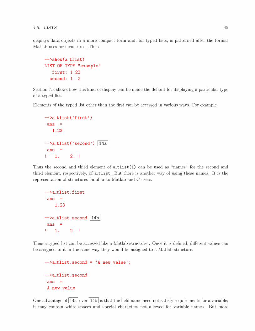
displays data objects in a more compact form and, for typed lists, is patterned after the formatMatlab uses for structures. Thus
-->show(a tlist)
LIST OF TYPE "example"
first: 1.23
second: 1 2
Section 7.3 shows how this kind of display can be made the default for displaying a particular typeof a typed list.
Elements of the typed list other than the first can be accessed in various ways. For example
-->a tlist(’first’)
ans =
1.23
-->a tlist(’second’) 14a
ans =
! 1. 2. !
Thus the second and third element of a tlist(1) can be used as “names” for the second andthird element, respectively, of a tlist. But there is another way of using these names. It is therepresentation of structures familiar to Matlab and C users.
-->a tlist.first
ans =
1.23
-->a tlist.second 14b
ans =
! 1. 2. !
Thus a typed list can be accessed like a Matlab structure . Once it is defined, different values canbe assigned to it in the same way they would be assigned to a Matlab structure.
-->a tlist.second = ’A new value’;
-->a tlist.second
ans =
A new value
One advantage of 14a over 14b is that the field name need not satisfy requirements for a variable;it may contain white spaces and special characters not allowed for variable names. But more
46 CHAPTER 4. VARIABLE TYPES
importantly, the field name may be computed by concatenating strings or it could be the elementof a string vector.
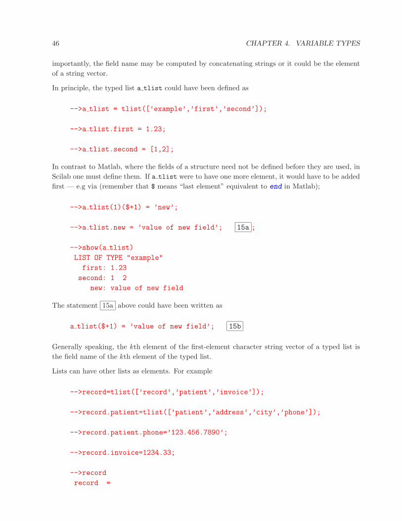
In principle, the typed list a tlist could have been defined as
-->a tlist = tlist([’example’,’first’,’second’]);
-->a tlist.first = 1.23;
-->a tlist.second = [1,2];
In contrast to Matlab, where the fields of a structure need not be defined before they are used, inScilab one must define them. If a tlist were to have one more element, it would have to be addedfirst — e.g via (remember that $ means “last element” equivalent to end in Matlab);
-->a tlist(1)($+1) = ’new’;
-->a tlist.new = ’value of new field’; 15a ;
-->show(a tlist)
LIST OF TYPE "example"
first: 1.23
second: 1 2
new: value of new field
The statement 15a above could have been written as
a tlist($+1) = ’value of new field’; 15b
Generally speaking, the kth element of the first-element character string vector of a typed list isthe field name of the kth element of the typed list.
Lists can have other lists as elements. For example
-->record=tlist([’record’,’patient’,’invoice’]);
-->record.patient=tlist([’patient’,’address’,’city’,’phone’]);
-->record.patient.phone=’123.456.7890’;
-->record.invoice=1234.33;
-->record
record =
4.5. LISTS 47
record(1)
!record patient invoice !
record(2)
record(2)(1)
!patient address city phone !
record(2)(2)
Undefined
record(2)(3)
Undefined
record(2)(4)
123.456.7890
record(3)
1234.33
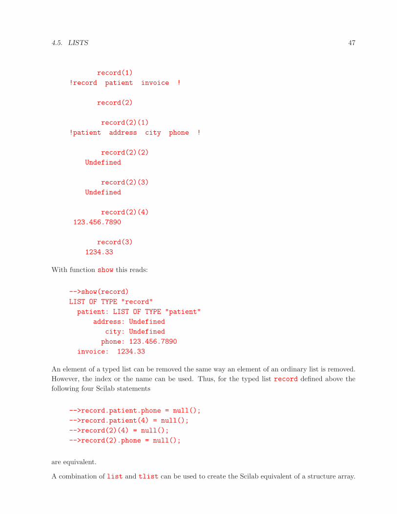
With function show this reads:
-->show(record)
LIST OF TYPE "record"
patient: LIST OF TYPE "patient"
address: Undefined
city: Undefined
phone: 123.456.7890
invoice: 1234.33
An element of a typed list can be removed the same way an element of an ordinary list is removed.However, the index or the name can be used. Thus, for the typed list record defined above thefollowing four Scilab statements
-->record.patient.phone = null();
-->record.patient(4) = null();
-->record(2)(4) = null();
-->record(2).phone = null();
are equivalent.
A combination of list and tlist can be used to create the Scilab equivalent of a structure array.

48 CHAPTER 4. VARIABLE TYPES
-->seis1 =
tlist([’seismic’,’first’,’last’,’step’,’traces’,’units’],0,[],4,[],’ms’);
-->seismic = list(seis1,seis1,seis1);
-->for ii=1:3
--> seismic(ii).last=1000*ii;
--> nsamp = (seismic(ii).last-seismic(ii).first)/seismic(ii).step+1;
--> seismic(ii).traces=rand(nsamp,10);
-->end
-->show(seismic)
List element 1:
LIST OF TYPE "seismic"
first: 0
last: 1000
step: 4
traces: 251 by 10 matrix
units: ms
List element 2:
LIST OF TYPE "seismic"
first: 0
last: 2000
step: 4
traces: 501 by 10 matrix
units: ms
List element 3:
LIST OF TYPE "seismic"
first: 0
last: 3000
step: 4
traces: 751 by 10 matrix
units: ms
Thus seismic is a list with three seismic data sets with the same start times but different endtimes, that can be individually addressed.
-->show(seismic(3))
LIST OF TYPE "seismic"
first: 0
last: 3000
step: 4
traces: 751 by 10 matrix

4.5. LISTS 49
units: ms
It is also straight forward to access fields of individual data sets. For example,
-->seismic(2).last
ans =
2000.
4.5.3 Matrix-oriented typed lists (mlist)
Help file and manuals provide only very sketchy information about matrix-oriented typed lists. Anmlist is defined like a regular typed list discussed above. This is illustrated by an example. Thestatement
-->an mlist=mlist([’VVV’,’name’,’value’],[’a’,’b’,’c’],[1 2 3])
an mlist =
an mlist(1)
!VVV name value !
an mlist(2) 16a
!a b c !
an mlist(3)
! 1. 2. 3. !
creates a matrix-like typed list, and the statements
-->an mlist.name
ans = !a b c !
-->an mlist(’name’)
ans =
!a b c !
-->an mlist.value
ans =
! 1. 2. 3. !
-->an mlist(’value’)
ans =
! 1. 2. 3. !
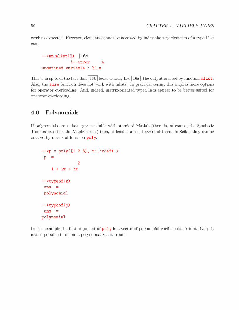
50 CHAPTER 4. VARIABLE TYPES
work as expected. However, elements cannot be accessed by index the way elements of a typed listcan.
-->an mlist(2) 16b
!--error 4
undefined variable : %l e
This is in spite of the fact that 16b looks exactly like 16a , the output created by function mlist.Also, the size function does not work with mlists. In practical terms, this implies more optionsfor operator overloading. And, indeed, matrix-oriented typed lists appear to be better suited foroperator overloading.
4.6 Polynomials
If polynomials are a data type available with standard Matlab (there is, of course, the SymbolicToolbox based on the Maple kernel) then, at least, I am not aware of them. In Scilab they can becreated by means of function poly.
-->p = poly([1 2 3],’z’,’coeff’)
p =
2
1 + 2z + 3z
-->typeof(z)
ans =
polynomial
-->typeof(p)
ans =
polynomial
In this example the first argument of poly is a vector of polynomial coefficients. Alternatively, itis also possible to define a polynomial via its roots.
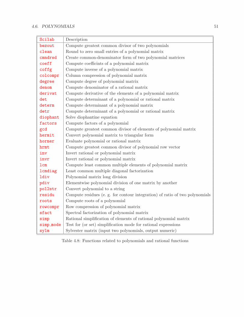
4.6. POLYNOMIALS 51
Scilab Descriptionbezout Compute greatest common divisor of two polynomialsclean Round to zero small entries of a polynomial matrixcmndred Create common-denominator form of two polynomial matricescoeff Compute coefficints of a polynomial matrixcoffg Compute inverse of a polynomial matrixcolcompr Column compression of polynomial matrixdegree Compute degree of polynomial matrixdenom Compute denominator of a rational matrixderivat Compute derivative of the elements of a polynomial matrixdet Compute determinant of a polynomial or rational matrixdeterm Compute determinant of a polynomial matrixdetr Compute determinant of a polynomial or rational matrixdiophant Solve diophantine equationfactors Compute factors of a polynomialgcd Compute greatest common divisor of elements of polynomial matrixhermit Convert polynomial matrix to triangular formhorner Evaluate polynomial or rational matrixhrmt Compute greatest common divisor of polynomial row vectorinv Invert rational or polynomial matrixinvr Invert rational or polynomial matrixlcm Compute least common multiple elements of polynomial matrixlcmdiag Least common multiple diagonal factorizationldiv Polynomial matrix long divisionpdiv Elementwise polynomial division of one matrix by anotherpol2str Convert polynomial to a stringresidu Compute residues (e. g. for contour integration) of ratio of two polynomialsroots Compute roots of a polynomialrowcompr Row compression of polynomial matrixsfact Spectral factorization of polynomial matrixsimp Rational simplification of elements of rational polynomial matrixsimp mode Test for (or set) simplification mode for rational expressionssylm Sylvester matrix (input two polynomials, output numeric)
Table 4.8: Functions related to polynomials and rational functions
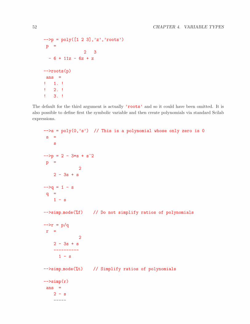
52 CHAPTER 4. VARIABLE TYPES
-->p = poly([1 2 3],’z’,’roots’)
p =
2 3
- 6 + 11z - 6z + z
-->roots(p)
ans =
! 1. !
! 2. !
! 3. !
The default for the third argument is actually ’roots’ and so it could have been omitted. It isalso possible to define first the symbolic variable and then create polynomials via standard Scilabexpressions.
-->s = poly(0,’s’) // This is a polynomial whose only zero is 0
s =
s
-->p = 2 - 3*s + s2p =
2
2 - 3s + s
-->q = 1 - s
q =
1 - s
-->simp mode(%f) // Do not simplify ratios of polynomials
-->r = p/q
r =
2
2 - 3s + s
----------
1 - s
-->simp mode(%t) // Simplify ratios of polynomials
-->simp(r)
ans =
2 - s
-----

4.6. POLYNOMIALS 53
1
-->type(r)
ans =
16.
-->typeof(r)
ans =
rational
The result of type indicates that r is a typed list and typeof tells us that it is a list of typerational.
Table 4.8 lists functions available in Scilab for manipulating polynomials and ratios of polynomials.
One difference between computer algebra packages such as Mathematica, Maple, or Macsyma andthis implementation of polynomial algebra is the precision. Scilab evaluates expression to its normalprecision while the above packages maintain infinite precision unless requested to perform numericalevaluations.
Chapter 5
Functions
5.1 General
For someone coming from Matlab Scilab functions are familiar entities. One difference is thatparentheses are generally required even if a function has no input arguments. There are twoexceptions:
• The function is treated as a variable
• The function has at most one output argument and all input arguments are strings (command-type syntax).
Command-style Syntax: For any function that has at most one output argument and whoseinput arguments are character strings, the calling syntax may be simplified by dropping the paren-theses. Thus
-->getf(’fun1.sci’)
-->getf ’fun1.sci’
-->getf fun1.sci // Command-style syntax
are equivalent. The last form represents the command-style syntax (a command, possibly followedby one or more arguments; Matlab has a similar feature). More generally, if function funct acceptsthree string arguments then
funct(’a’,’total’,’of three strings’)
is equivalent to
funct a total ’of three strings’
54

5.1. GENERAL 55
Here the quotes around the last argument are required to prevent it from being interpreted as threeindividual strings. It even seems to work if the function accepts non-string arguments providedthat these arguments are optional. In order to run a script, say script.sce, the commandexec(’script.sce’) must be executed. The function exec has one required and two optionalarguments (one of which is numeric). Nevertheless,
exec(’script.sce’)
exec ’script.sce’
exec script.sce
give all the same result.
Scilab provides one way of passing parameters to a function that is not available in Matlab: namedarguments. This method of passing arguments is especially practical with function that have manyinput parameters with good default values — plot functions are typical examples. For example,the built-in function plot2d can be called as follows
plot2d([logflag],x,y,[style,strf,leg,rect,nax])
The first argument is an optional string that can be used to set axis graduation (linear or logarith-mic). The next two arguments are the x-coordinate and y-coordinate of the function to be plotted.The last five arguments are optional again. Now suppose one wants to use the default values forall optional parameters except the curve legend (parameter leg). The parameter logflag is nota problem. If the first input argument is not a string the program knows it is not given as apositional parameter. But the defaults of style and strf would have to be given so that leg isat the correct position in the argument list. Hence, the statement would read as follows
-->plot2d(x,y,1,’161’,’Curve legend’)
This, of course means that one has to figure out what the default values are. The simpler solutionto this problem is to use named parameters
-->plot2d(x,y,leg=’Curve legend’)
Note that the name of the argument, leg is not quoted — it is not a string. The order of namedparameters is arbitrary, but any positional parameters must come before named parameters. It isfor example possible to specify the parameter logflag after all. For example,
-->plot2d(x,y,leg=’Curve legend’,logflag=’ll’)
creates the same plot, but with log-log axes. Of course, the same could be achieved by
-->plot2d(’ll’,x,y,leg=’Curve legend’)
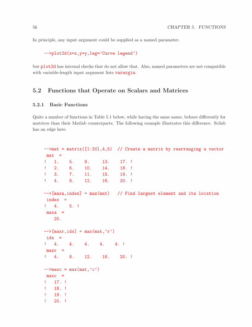
56 CHAPTER 5. FUNCTIONS
In principle, any input argument could be supplied as a named parameter.
-->plot2d(x=x,y=y,leg=’Curve legend’)
but plot2d has internal checks that do not allow that. Also, named parameters are not compatiblewith variable-length input argument lists varargin.
5.2 Functions that Operate on Scalars and Matrices
5.2.1 Basic Functions
Quite a number of functions in Table 5.1 below, while having the same name, behave differently formatrices than their Matlab counterparts. The following example illustrates this difference. Scilabhas an edge here.
-->mat = matrix([1:20],4,5) // Create a matrix by rearranging a vector
mat =
! 1. 5. 9. 13. 17. !
! 2. 6. 10. 14. 18. !
! 3. 7. 11. 15. 19. !
! 4. 8. 12. 16. 20. !
-->[maxa,index] = max(mat) // Find largest element and its location
index =
! 4. 5. !
maxa =
20.
-->[maxr,idx] = max(mat,’r’)
idx =
! 4. 4. 4. 4. 4. !
maxr =
! 4. 8. 12. 16. 20. !
-->maxc = max(mat,’c’)
maxc =
! 17. !
! 18. !
! 19. !
! 20. !

5.2. FUNCTIONS THAT OPERATE ON SCALARS AND MATRICES 57
Scilab Descriptionabs(a) Absolute value of a, |a|bool2s Replace %t (or non-zero entry) in matrix by 1 and %f by zeroceil(a) Round the elements of a to the nearest integers ≥aclean “Clean” matrices; i.e. small entries are set to zeroconj Complex conjugatecumprod Cumulative product of all elements of a vector or arraycumsum Cumulative sum of all elements of a vector or arrayfix(a) Rounds the elements of a to the nearest integers towards zerofloor(a) Rounds the elements of a to the nearest integers ≥ a
gsort(a) Sort elements/rows/columns of aimag Imaginary part of a matrixintersect(str1,str2) Returns elements common to two vectors str1 and str2
lex sort Sort rows of matrices in lexicographic orderlinspace Create vector with linearly spaced elementslogspace Create vector with logarithmically spaced elementsmax Maximum of all elements of a vector or arraymaxi Maximum of all elements of a vector or arraymean Mean of all elements of a vector or arraymedian Median of all elements of a vector or arraymin Minimum of all elements of a vector or arraymini Minimum of all elements of a vector or arraymodulo(a,b) a-b.*fix(a./b) if b∼=0; remainder of a divided by b
pmodulo(a,b) a-b.*floor(a./b) if b∼=0; remainder of a divided by b
prod Product of the elements of a matrixreal Real part of a matrixround(a) Round the elements of a to the nearest integerssign(a) Signum function, a/|a| for a 6= 0sqrt(a)
√a
st deviation Standard deviationsum Sum of all elements of a matrixunion(a,b) Extract the unique common elements of a and b
unique(a) Return the unique elements of a in ascending order
Table 5.1: Basic arithmetic functions
There is no equivalent in Matlab for the behavior of max(mat). It is particular the easy way ofgetting the indices of the largest element of a matrix that I consider extremely useful. The Matlabversion of max behaves just like max(mat,’r’) does — it computes a row vector representing themaxima of every column. Likewise, max(mat,’c’) computes a column vector with the maximumelement in each row (equivalent to max(mat,[],2) in Matlab).
The analogous behavior is found for Scilab functions cumprod, cumsum, maxi, mean, median, min,mini, prod, sum, and st deviation. The functions max and maxi are equivalent as are min andmini.
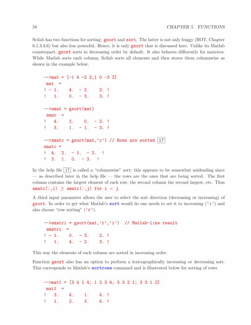
58 CHAPTER 5. FUNCTIONS
Scilab has two functions for sorting: gsort and sort. The latter is not only buggy (BOT, Chapter6.1.3.3.6) but also less powerful. Hence, it is only gsort that is discussed here. Unlike its Matlabcounterpart, gsort sorts in decreasing order by default. It also behaves differently for matrices.While Matlab sorts each column, Scilab sorts all elements and then stores them columnwise asshown in the example below.
-->mat = [-1 4 -2 2;1 0 -3 3]
mat =
! - 1. 4. - 2. 2. !
! 1. 0. - 3. 3. !
-->smat = gsort(mat)
smat =
! 4. 2. 0. - 2. !
! 3. 1. - 1. - 3. !
-->smatc = gsort(mat,’c’) // Rows are sorted 17
smatc =
! 4. 2. - 1. - 2. !
! 3. 1. 0. - 3. !
In the help file 17 is called a “columnwise” sort; this appears to be somewhat misleading since— as described later in the help file — the rows are the ones that are being sorted. The firstcolumn contains the largest element of each row, the second column the second largest, etc. Thussmatc(:,i) ≥ smatc(:,j) for i < j.
A third input parameter allows the user to select the sort direction (decreasing or increasing) ofgsort. In order to get what Matlab’s sort would do one needs to set it to increasing (’i’) andalso choose “row sorting” (’r’).
-->smatri = gsort(mat,’r’,’i’) // Matlab-like result
smatri =
! - 1. 0. - 3. 2. !
! 1. 4. - 2. 3. !
This way the elements of each column are sorted in increasing order.
Function gsort also has an option to perform a lexicographically increasing or decreasing sort.This corresponds to Matlab’s sortrows command and is illustrated below for sorting of rows
-->mat1 = [3 4 1 4; 1 2 3 4; 3 3 2 1; 3 3 1 2]
mat1 =
! 3. 4. 1. 4. !
! 1. 2. 3. 4. !
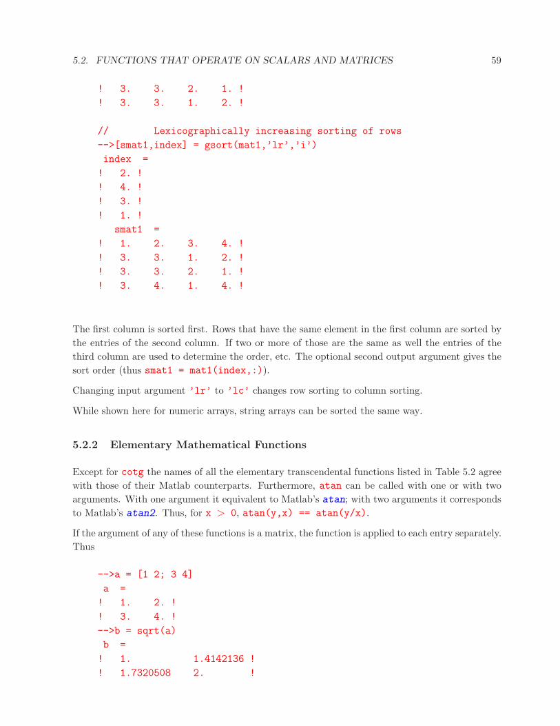
5.2. FUNCTIONS THAT OPERATE ON SCALARS AND MATRICES 59
! 3. 3. 2. 1. !
! 3. 3. 1. 2. !
// Lexicographically increasing sorting of rows
-->[smat1,index] = gsort(mat1,’lr’,’i’)
index =
! 2. !
! 4. !
! 3. !
! 1. !
smat1 =
! 1. 2. 3. 4. !
! 3. 3. 1. 2. !
! 3. 3. 2. 1. !
! 3. 4. 1. 4. !
The first column is sorted first. Rows that have the same element in the first column are sorted bythe entries of the second column. If two or more of those are the same as well the entries of thethird column are used to determine the order, etc. The optional second output argument gives thesort order (thus smat1 = mat1(index,:)).
Changing input argument ’lr’ to ’lc’ changes row sorting to column sorting.
While shown here for numeric arrays, string arrays can be sorted the same way.
5.2.2 Elementary Mathematical Functions
Except for cotg the names of all the elementary transcendental functions listed in Table 5.2 agreewith those of their Matlab counterparts. Furthermore, atan can be called with one or with twoarguments. With one argument it equivalent to Matlab’s atan; with two arguments it correspondsto Matlab’s atan2. Thus, for x > 0, atan(y,x) == atan(y/x).
If the argument of any of these functions is a matrix, the function is applied to each entry separately.Thus
-->a = [1 2; 3 4]
a =
! 1. 2. !
! 3. 4. !
-->b = sqrt(a)
b =
! 1. 1.4142136 !
! 1.7320508 2. !
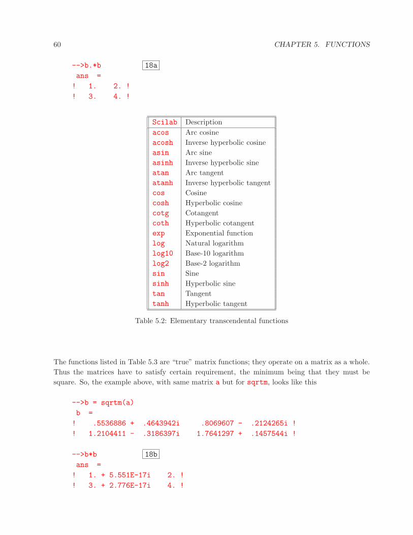
60 CHAPTER 5. FUNCTIONS
-->b.*b 18a
ans =
! 1. 2. !
! 3. 4. !
Scilab Descriptionacos Arc cosineacosh Inverse hyperbolic cosineasin Arc sineasinh Inverse hyperbolic sineatan Arc tangentatanh Inverse hyperbolic tangentcos Cosinecosh Hyperbolic cosinecotg Cotangentcoth Hyperbolic cotangentexp Exponential functionlog Natural logarithmlog10 Base-10 logarithmlog2 Base-2 logarithmsin Sinesinh Hyperbolic sinetan Tangenttanh Hyperbolic tangent
Table 5.2: Elementary transcendental functions
The functions listed in Table 5.3 are “true” matrix functions; they operate on a matrix as a whole.Thus the matrices have to satisfy certain requirement, the minimum being that they must besquare. So, the example above, with same matrix a but for sqrtm, looks like this
-->b = sqrtm(a)
b =
! .5536886 + .4643942i .8069607 - .2124265i !
! 1.2104411 - .3186397i 1.7641297 + .1457544i !
-->b*b 18b
ans =
! 1. + 5.551E-17i 2. !
! 3. + 2.776E-17i 4. !

5.2. FUNCTIONS THAT OPERATE ON SCALARS AND MATRICES 61
clean(b*b) 19
ans =
! 1. 2. !
! 3. 4. !
Obviously, the matrix b is complex and so rounding errors lead to small imaginary parts of someof the entries in the product b*b. Expression 19 illustrates how function clean can be used toremove such small matrix entries.
The important difference between these two examples is that in 18a corresponding entries of bare multiplied (the . in front of the *) whereas in 18b the matrices are multiplied.
The list of functions in Table 5.3 is longer than it would be in Matlab; on the other hand Scilablacks an equivalent for Matlab’s funm function which works for any user-specified functions; forgood accuracy, matrices should be symmetric or Hermitian.
Scilab Descriptionacoshm Matrix inverse hyperbolic cosineacosm Matrix arc cosineasinhm Matrix inverse hyperbolic sineatanhm Matrix inverse hyperbolic tangentatanhm Matrix inverse hyperbolic tangentcoshm Matrix hyperbolic cosinecosm Matrix cosineexpm Matrix xponential functionlogm Matrix natural logarithmsinhm Matrix hyperbolic sinesinm Matrix sinesqrtm Matrix square roottanhm Matrix hyperbolic tangenttanm Matrix tangent
Table 5.3: Matrix functions
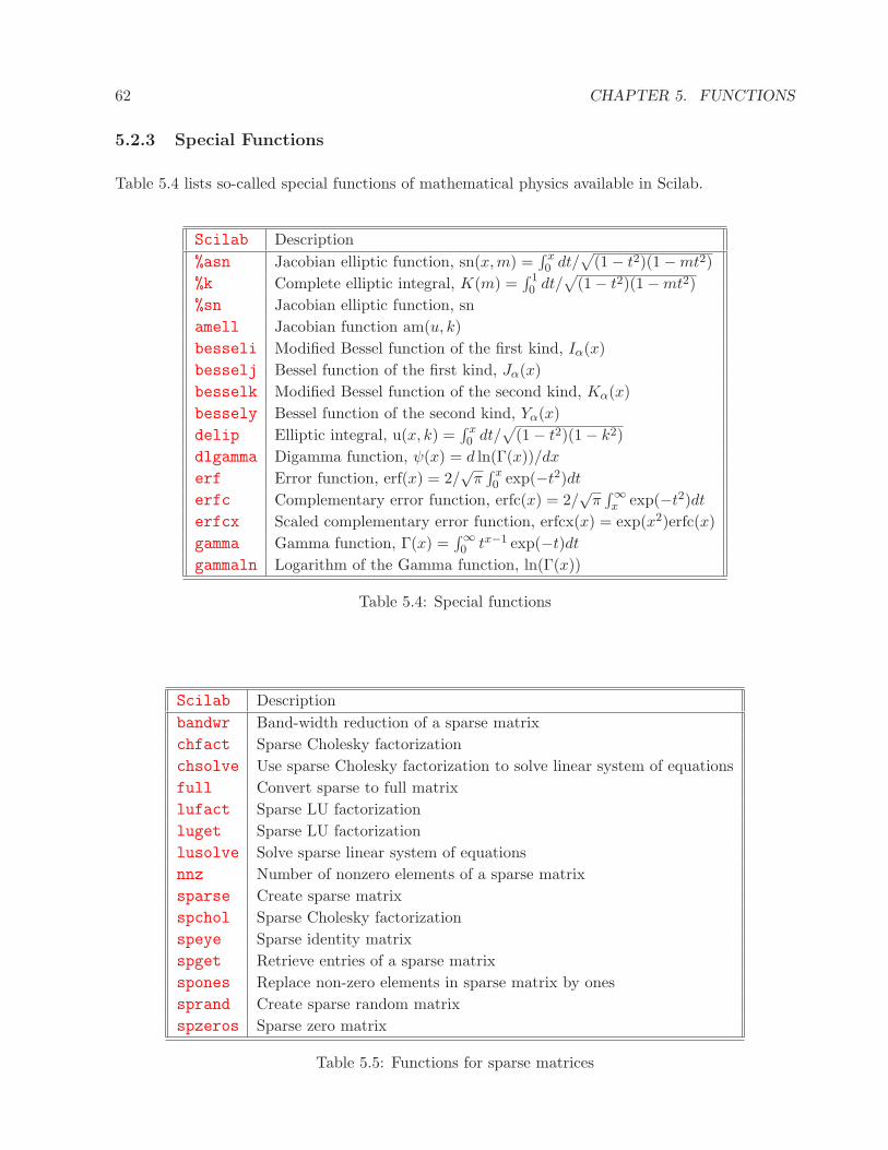
62 CHAPTER 5. FUNCTIONS
5.2.3 Special Functions
Table 5.4 lists so-called special functions of mathematical physics available in Scilab.
Scilab Description%asn Jacobian elliptic function, sn(x,m) =
∫ x0 dt/
√(1− t2)(1−mt2)
%k Complete elliptic integral, K(m) =∫ 10 dt/
√(1− t2)(1−mt2)
%sn Jacobian elliptic function, snamell Jacobian function am(u, k)besseli Modified Bessel function of the first kind, Iα(x)besselj Bessel function of the first kind, Jα(x)besselk Modified Bessel function of the second kind, Kα(x)bessely Bessel function of the second kind, Yα(x)delip Elliptic integral, u(x, k) =
∫ x0 dt/
√(1− t2)(1− k2)
dlgamma Digamma function, ψ(x) = d ln(Γ(x))/dx
erf Error function, erf(x) = 2/√
π∫ x0 exp(−t2)dt
erfc Complementary error function, erfc(x) = 2/√
π∫∞x exp(−t2)dt
erfcx Scaled complementary error function, erfcx(x) = exp(x2)erfc(x)gamma Gamma function, Γ(x) =
∫∞0 tx−1 exp(−t)dt
gammaln Logarithm of the Gamma function, ln(Γ(x))
Table 5.4: Special functions
Scilab Descriptionbandwr Band-width reduction of a sparse matrixchfact Sparse Cholesky factorizationchsolve Use sparse Cholesky factorization to solve linear system of equationsfull Convert sparse to full matrixlufact Sparse LU factorizationluget Sparse LU factorizationlusolve Solve sparse linear system of equationsnnz Number of nonzero elements of a sparse matrixsparse Create sparse matrixspchol Sparse Cholesky factorizationspeye Sparse identity matrixspget Retrieve entries of a sparse matrixspones Replace non-zero elements in sparse matrix by onessprand Create sparse random matrixspzeros Sparse zero matrix
Table 5.5: Functions for sparse matrices

5.2. FUNCTIONS THAT OPERATE ON SCALARS AND MATRICES 63
5.2.4 Linear Algebra
Tables 5.5 and 5.6 list functions for linear-algebra operations. Functions for full matrices work onsparse matrices as well.
Scilab Descriptionbalanc Balance matrix to improve condition numberbdiag Block diagonalization of matrixbdiag(M) Block diagonalization/generalized eigenvectors of Mchol(M) Choleski factorization; R’*R = M
colcomp(M) Column compression of Mcond Condition number of Mdet Determinant of a matrixfullrf(M) Full-rank factorization of Mfullrfk(M) Full-rank factorization of MK
givens Given’s rotationhess(M) Hessenberg form of Mhouseholder Householder orthogonal reflection matrixinv(M) Inverse of matrix M
kernel(M) Nullspace of Mlinsolve Linear-equation solvernorm(M) Norm of M (matrix or vector)orth(M) Orthogonal basis for the range of Mpinv(M) Pseudoinverse of Mpolar(M) Polar form of M, M=R*expm(%i*Theta)qr(M) QR decomposition of Mrange(M) Range of Mrank(M) Rank of Mrcond(M) Reciprocal of the condition number of M; L-1 normschur(M) Schur decompositionspaninter(M,N) Intersection of the span of M and N
spanplus(M,N) Span of M and N
spec Eigenvalues of matrixsva(M) Singular-value approximation of M for specified ranksvd(M) Singular-value decomposition of Mtrace(M) Trace (sum of diagonal elements) of M
Table 5.6: Linear algebra
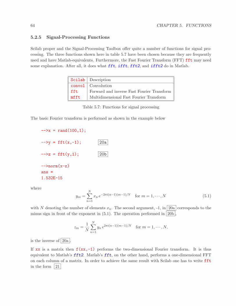
64 CHAPTER 5. FUNCTIONS
5.2.5 Signal-Processing Functions
Scilab proper and the Signal-Processing Toolbox offer quite a number of functions for signal pro-cessing. The three functions shown here in table 5.7 have been chosen because they are frequentlyused and have Matlab-equivalents. Furthermore, the Fast Fourier Transform (FFT) fft may needsome explanation. After all, it does what fft, ifft, fft2, and ifft2 do in Matlab.
Scilab Descriptionconvol Convolutionfft Forward and inverse Fast Fourier Transformmfft Multidimensional Fast Fourier Transform
Table 5.7: Functions for signal processing
The basic Fourier transform is performed as shown in the example below
-->x = rand(100,1);
-->y = fft(x,-1); 20a
-->z = fft(y,1); 20b
-->norm(x-z)
ans =
1.532E-15
where
ym =N∑
n=1
xn e−2πi(n−1)(m−1)/N for m = 1, · · · , N (5.1)
with N denoting the number of elements xn. The second argument, -1, in 20a corresponds to theminus sign in front of the exponent in (5.1). The operation performed in 20b ,
zm =1N
N∑
n=1
yn e2πi(n−1)(m−1)/N for m = 1, · · · , N,
is the inverse of 20a .
If xx is a matrix then f(xx,-1) performs the two-dimensional Fourier transform. It is thusequivalent to Matlab’s fft2. Matlab’s fft, on the other hand, performs a one-dimensional FFTon each column of a matrix. In order to achieve the same result with Scilab one has to write fftin the form 21
5.2. FUNCTIONS THAT OPERATE ON SCALARS AND MATRICES 65
-->n = 100; m = 20;
-->xx = rand(n,m);
-->yy1 = zeros(xx);
-->for i=1:m
--> yy1(:,i) = fft(xx(:,i),-1);
-->end
-->yy2 = fft(xx,-1,n,1); 21
-->norm(yy1-yy2) 22
ans =
0.
-->zz = fft(yy2,1,n,1); 23
-->norm(xx-zz) 24
ans =
3.368E-15
Expression 22 shows that yy1 and yy2 are identical. Likewise, expression 24 shows that theinverse Fourier transform 23 works as expected with this syntax.
Furthermore, with yy2 computed in 21 , statement 25 computes the two-dimensional FFT of xx:
-->uu1 = fft(xx,-1); // Two-dimensional FFT of xx
-->uu2 = fft(yy2,-1,m,n); 25
-->norm(uu1-uu2)
ans =
0.
Obviously, uu1 and uu2 are identically.
66 CHAPTER 5. FUNCTIONS
5.3 File Input and Output
There are quite a few functions for formatted and unformatted reading and writing of text andnumeric data. Some have Matlab equivalents. They are summarized in tables 5.9 (reading), 5.10(writing), and 5.8 (ancillary functions). Many I/O functions come in pairs — one is designed toread what the other one writes. The special-purpose routines for, say, writing and reading audiofiles fall into this category. Some of the following pairs represent my own way of grouping. Thisgrouping does not imply that no other function can read what one of these functions writes andvice versa; rather, these pairs appear similar in terms of design philosophy and input arguments.
5.3.1 Opening and Closing of Files
Before one can read from, or write to, a file the file needs to be “opened”. This is transparentfor I/O functions, such as fprintfMat or fscanfMat, that only use a file name to specify whichfile to read from (write to). They open the requested file, read/write the data and close the filewithout the user being aware of it. But whenever there is a need to incrementally read or writedata it is up to the user to open files. A situation like that occurs, for example, with big data sets.One might read a piece of the data from file A, process it, and write it out to file B; then read in thenext piece of data from file A, process it, and write it to file B, etc. In this case files A and B mustbe opened before anything can be read from respectively written to them. Scilab has two functionsfor opening a file, mopen and file, and Scilab functions that allow incremental I/O require oneor the other. For this reason the subsequent discussion of specific I/O functions mentions, whereappropriate, which one of the two functions needs to be used for opening a file. Function mopen isquite similar to Matlab’s fopen whereas file reminds one of the Fortran equivalent.
Functions mopen and file output a file identifier (Matlab terminology). Scilab help files call it“file descriptor” or ”logical unit descriptor”; in Fortran it is called “Logical Unit Number”. It isthis file identifier, and not the file name, that is then used to specify from which file to read (towhich file to write). File identifiers are numbers which range from 1 to 19 in Scilab-2.6 for Windows.File identifier 1 is used for the history file scilab.hist, file identifiers 5 and 6 (%io(1) and %io(2),respectively) are reserved for keyboard (input) and Scilab window (output), respectively. Hence, amaximum of 16 file identifiers are available to users; this limits to 16 the number of user files thatcan be open at any one time.
Files that have been opened with mopen must be closed with mclose, and file with the ’close’option must be used to close files that have been opened with file. Examples of the use of mopen,mclose, and file are part of the discussion of specific I/O functions below.

5.3. FILE INPUT AND OUTPUT 67
Scilab Descriptiondispfiles Display properties of opened filesfile Open/close a file, define file attributesfileinfo Get information about a filegetio Get Scilab’s standard logical input/output unitsmclearerr Reset binary-file access errorsmclose Close (all) open file(s)meof Check if end-of-file has been reachedmopen Open a filemseek Set position in a binary filemtell Output the current position in a binary filenewest Find newest of a set of filesxgetfile Open dialog box for file selection
Table 5.8: Functions that open, querry, manipulate, and close files
5.3.2 Functions mgetl and mputl
Function mputl writes a vector of strings to an ASCII file in form of a sequence of lines, and mgetl
can retrieve one or more of these lines. This is a simple example:
-->text = [’This is line 1’;’Line 2 ’;’Line 3 (last)’]
text =
!This is line 1 !
! !
!Line 2 !
! !
!Line 3 (last) !
-->mputl(text,’C:\temp\dummy.txt’)-->
-->all = mgetl(’C:\temp\dummy.txt’) // Get the whole file
all =
!This is line 1 !
! !
!Line 2 !
! !
!Line 3 (last) !
With only one input argument, mgetl reads the whole file. If only the first few lines are requiredthe number of lines can be specified via the second input parameter:

68 CHAPTER 5. FUNCTIONS
Scilab Descriptionauread Read a .au audio file from diskexcel2sci Read ASCII file created by MS Excelfscanf Read numeric/string variables from ASCII file under format controlfscanfMat Read matrix from ASCII fileinput Read from keyboard with a prompt message to Scilab windowload Load variables previously saved with save
loadwave Read a .wav sound filemfscanf Read data from file (C-type format)mget Read numeric data (vector) from binary file (conversion format)mgeti Read data from binary file, converts to Scilab integer formatmgetl Read a specified number of lines from ASCII filemgetstr Read bytes from binary or ASCII file and interpret as character stringmscanf Read data from keyboard (C-type format)mtlb load Load variables from file with Matlab-4 formatread Read matrix of strings/numbers from ASCII file under format controlread4b Read Fortran binary file (4 bytes/word)readb Read Fortran binary file (8 byte/word)readc Read a character string from a file/keyboardsave Save current Scilab variables in binary filewavread Read a .wav sound file
Table 5.9: Functions that input data from files or keyboard
-->only2 = mgetl(’C:\temp\dummy.txt’,2) // Read first 2 lines only
only2 =
!This is line 1 !
! !
!Line 2 !
If more lines are requested than are available, the function aborts with an error message. If thesecond argument is -1, all lines are read (equivalent to no second input argument).
In the examples above the file to use is identified by it name. In a case like this mgetl does threethings. It opens the file for reading, reads the lines requested, and closes the file again. Thisconvenience comes at a price. It is not possible to read a file a few lines at a time. If this isnecessary you must open the file yourself and use the file identifier created by mopen to specify thefile to mgetl. Finally, once you are done reading, you need to close the file again.
fid = mopen(’C:\temp\dummy.txt’,’r’) // Open file for reading
fid =
3.
-->one = mgetl(fid,1) // Read one line
one =

5.3. FILE INPUT AND OUTPUT 69
Scilab Descriptionauwrite Write a .au audio file to diskdiary Write screen output of a Scilab session to a filedisp Write input argument to Scilab windowfprintf Write formatted data to file (like C-language fprintf function)fprintfMat Write matrix to ASCII file under format controlmfprintf Write data to ASCII file (C-type format)mprintf Writes data to Scilab window (C-type format)mput Write numeric data to file in user-specified binary representationmputl Write string vector to ASCII file (one line per vector element)mputstr Write character string to an ASCII filemtlb save Save variables to file in Matlab-4 formatprint Print variables to file in the format used for Scilab windowprintf Print to Scilab window (emulation of C-language printf function)savewave Write a .wav sound filewavwrite Write a .wav sound filewritb Write matrix in to a Fortran binary file (4 bytes/word)write Write matrix of strings/numbers to ASCI file (Fortran-type format)write4b Write matrix in to a Fortran binary file (8 bytes/word)
Table 5.10: Functions that output data to files or to the Scilab window
This is line 1
-->twomore = mgetl(fid,2) // Read two more lines
twomore =
!Line 2 !
! !
!Line 3 (last) !
-->mclose(fid) // Close the file
ans =
0.
An analogous procedure can be used to write a file one line (or several lines) at a time.
It is important to note that mputl puts each string in a string matrix in a separate line. Thus astring matrix with more than one column — when read in — will become a one-column matrix.This is illustrated in the next example. 26a
-->textlines = [’This is line 1a’,’Line 1b’;
--> ’This is line 2a’,’Line 2b’]
textlines =
!This is line 1a Line 1b !
! !
!This is line 2a Line 2b !
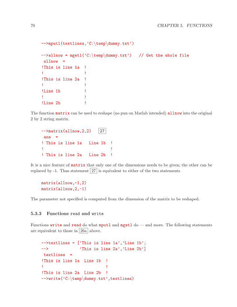
70 CHAPTER 5. FUNCTIONS
-->mputl(textlines,’C:\temp\dummy.txt’)
-->allnow = mgetl(’C:\temp\dummy.txt’) // Get the whole file
allnow =
!This is line 1a !
! !
!This is line 2a !
! !
!Line 1b !
! !
!Line 2b !
The function matrix can be used to reshape (no pun on Matlab intended) allnow into the original2 by 2 string matrix.
-->matrix(allnow,2,2) 27
ans =
! This is line 1a Line 1b !
! !
! This is line 2a Line 2b !
It is a nice feature of matrix that only one of the dimensions needs to be given; the other can bereplaced by -1. Thus statement 27 is equivalent to either of the two statements
matrix(allnow,-1,2)
matrix(allnow,2,-1)
The parameter not specified is computed from the dimension of the matrix to be reshaped.
5.3.3 Functions read and write
Functions write and read do what mputl and mgetl do — and more. The following statementsare equivalent to those in 26a above.
-->textlines = [’This is line 1a’,’Line 1b’;
--> ’This is line 2a’,’Line 2b’]
textlines =
!This is line 1a Line 1b !
! !
!This is line 2a Line 2b !
-->write(’C:\temp\dummy.txt’,textlines)

5.3. FILE INPUT AND OUTPUT 71
-->all = read(’C:\temp\dummy.txt’,-1,1,’(A)’) // Get the whole file
all =
! This is line 1a !
! !
! This is line 2a !
! !
! Line 1b !
! !
! Line 2b !
While the write statements only needs the file name and the data the read statement also wants thesize of the array to read and a format in FORTRAN syntax. The dimension are in input arguments2 and 3, the -1 simply instructs read to read the whole file; in this example it could have beenreplaced by 4 since there are 4 strings in the file. Like mputl function write writes a string arrayone column to a line.
Functions read and write, when used with a file name as first argument, open the file and closeit again after the I/O operation. To read or write incrementally, one needs to open the file oneself.However, this cannot be done with function mopen used above. Rather, the file must be opened(and closed) with function file. This is illustrated in the example below where the file createdabove is read again.
-->fid = file(’open’,’C:\temp\dummy.txt’,’unknown’) // Open file
fid =
4.
-->one = read(fid,1,1,’(A)’) // Read one line
one =
This is line 1a
-->twomore = read(fid,2,1,’(A)’) // Read two more lines
twomore =
! This is line 2a !
! !
! Line 1b !
-->file(’close’,fid) // Close the file
Function file above opens the file C:\temp\dummy.txt for read and write access. By defaultthe file is a sequential-access file for ASCII data. Other file types can be chosen by setting theappropriate input parameters.
Sequentially writing to a file is completely analogous.
Functions read and write can also be used to read and write numeric data.
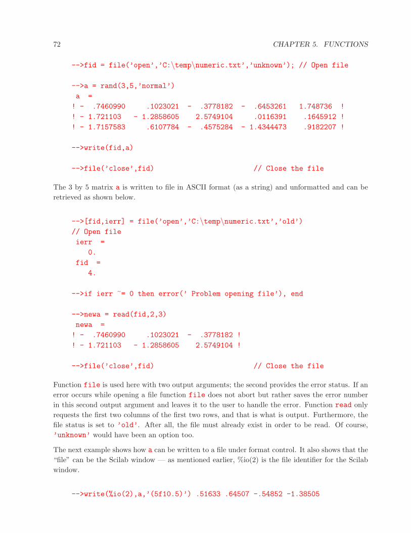
72 CHAPTER 5. FUNCTIONS
-->fid = file(’open’,’C:\temp\numeric.txt’,’unknown’); // Open file
-->a = rand(3,5,’normal’)
a =
! - .7460990 .1023021 - .3778182 - .6453261 1.748736 !
! - 1.721103 - 1.2858605 2.5749104 .0116391 .1645912 !
! - 1.7157583 .6107784 - .4575284 - 1.4344473 .9182207 !
-->write(fid,a)
-->file(’close’,fid) // Close the file
The 3 by 5 matrix a is written to file in ASCII format (as a string) and unformatted and can beretrieved as shown below.
-->[fid,ierr] = file(’open’,’C:\temp\numeric.txt’,’old’)// Open file
ierr =
0.
fid =
4.
-->if ierr ˜= 0 then error(’ Problem opening file’), end
-->newa = read(fid,2,3)
newa =
! - .7460990 .1023021 - .3778182 !
! - 1.721103 - 1.2858605 2.5749104 !
-->file(’close’,fid) // Close the file
Function file is used here with two output arguments; the second provides the error status. If anerror occurs while opening a file function file does not abort but rather saves the error numberin this second output argument and leaves it to the user to handle the error. Function read onlyrequests the first two columns of the first two rows, and that is what is output. Furthermore, thefile status is set to ’old’. After all, the file must already exist in order to be read. Of course,’unknown’ would have been an option too.
The next example shows how a can be written to a file under format control. It also shows that the“file” can be the Scilab window — as mentioned earlier, %io(2) is the file identifier for the Scilabwindow.
-->write(%io(2),a,’(5f10.5)’) .51633 .64507 -.54852 -1.38505
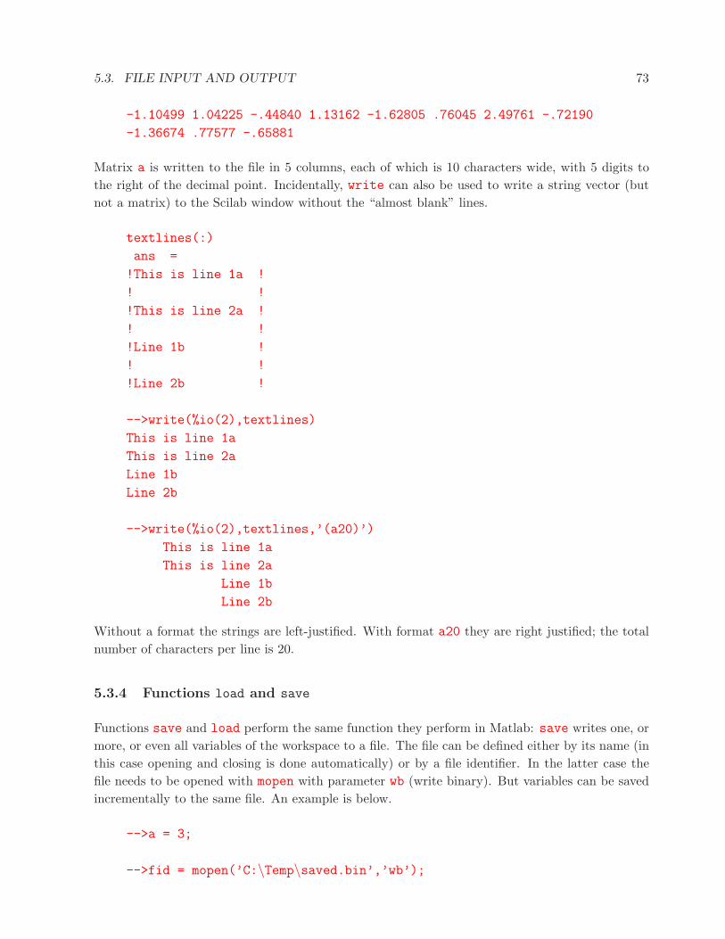
5.3. FILE INPUT AND OUTPUT 73
-1.10499 1.04225 -.44840 1.13162 -1.62805 .76045 2.49761 -.72190
-1.36674 .77577 -.65881
Matrix a is written to the file in 5 columns, each of which is 10 characters wide, with 5 digits tothe right of the decimal point. Incidentally, write can also be used to write a string vector (butnot a matrix) to the Scilab window without the “almost blank” lines.
textlines(:)
ans =
!This is line 1a !
! !
!This is line 2a !
! !
!Line 1b !
! !
!Line 2b !
-->write(%io(2),textlines)
This is line 1a
This is line 2a
Line 1b
Line 2b
-->write(%io(2),textlines,’(a20)’)
This is line 1a
This is line 2a
Line 1b
Line 2b
Without a format the strings are left-justified. With format a20 they are right justified; the totalnumber of characters per line is 20.
5.3.4 Functions load and save
Functions save and load perform the same function they perform in Matlab: save writes one, ormore, or even all variables of the workspace to a file. The file can be defined either by its name (inthis case opening and closing is done automatically) or by a file identifier. In the latter case thefile needs to be opened with mopen with parameter wb (write binary). But variables can be savedincrementally to the same file. An example is below.
-->a = 3;
-->fid = mopen(’C:\Temp\saved.bin’,’wb’);

74 CHAPTER 5. FUNCTIONS
-->save(fid,a)
-->b = 5; c = ’text’;
-->save(fid,b,c)
-->mclose(fid);
Note that variable names in the save command are not in quotes. In Matlab they would be.
To recall variables saved earlier, possibly in another session,
-->clear a, clear b
-->load(’C:\Temp\saved.bin’,’a’,’b’)
-->a,b
a =
3.
b =
5.
Here, as in Matlab’s load function, the variable names must be in quotes.
5.3.5 Functions mput and mget/mgeti
The two input functions allow one to read blocks of 1, 2, 4, or 8 bytes from a binary file andconvert them into either double-precision floating point numbers (mget) or into integers (mgeti)(see rightmost column of the table below). The type of conversion is controlled by a type parameterwhich can take the following values
Type in file in Scilabc 8-bit integer int8
s 16-bit integer int16
i 32-bit integer int32
l 64-bit integer double
uc Unsigned 8-bit integer uint8
us Unsigned 16-bit integer uint16
ui Unsigned 32-bit integer uint32
ul Unsigned 64-bit integer double
f 32-bit floating-point number double
d 64-bit floating-point number double

5.3. FILE INPUT AND OUTPUT 75
The functions can incrementally read/write files that have been opened with mopen.
With binary files the questions of byte ordering has to be addressed. Intel CPU’s, and thus PC’s,use “little-endian” byte ordering whereas so-called workstations (Sun Sparc, SGI, IBM RS/6000)use “big-endian” byte ordering. In Matlab byte ordering is specified when a file is opened withfopen. Function mopen in Scilab has no such option; instead, byte ordering is specified togetherwith the variable type by appending a b or l to the type parameter. Thus the statement for reading6 big-endian, 32-bit integers from a file with file identifier fid is
-->from file = mget(6,’ib’,fid)
Had the b been omitted the “natural” byte ordering of the computer on which the program runswould have been used (e.g. little-endian for a PC). As long as one reads files written on the sametype of computer byte ordering is generally not a problem. It needs attention when one reads a filecreated on a computer with different byte ordering.
5.3.6 Functions input and disp
Function input is completely equivalent to Matlab’s input:
-->response = input(’Prompt user for input’)
Prompt user for input-->3
response =
3.
The user response (3 in this example) can also be an expression involving variables in the workspace.Furthermore, by adding a second argument, ’string’ or simply ’s’, the user response can beinterpreted as a string. There is no need to put it in quotes.
Function disp has a close Matlab analog as well. Unlike its Matlab counterpart it can take morethan one argument. However, as illustrated out earlier (page 18) the arguments are displayed inreverse order.
5.3.7 Function xgetfile
Generally, functions whose name starts with an “x” have some connection to graphics (proba-bly some reference to Xwindows). This is also true for xgetfile which opens a dialog box forinteractive file selection. It works essentially like Matlab’s uigetfile. An example is
-->file name = xgetfile(filemask=’*.sgy’,dir=’D:\Data\Seismic’, ...
title=’Read SEG-Y file’);
which opens a file selection window with the title “Read SEG-Y file”. The initial directory shown inthe window is D:\Data\Seismic, and only files with file name extension .sgy are shown initially.

76 CHAPTER 5. FUNCTIONS
5.4 Utility Functions
This chapter describes some of the functions that are not directly necessary to run or debug Scilabfunctions, that are more peripheral to Scilab and do not fit well in any other topic discussedpreviously. Table 5.11 shows the functions I chose to put into this category.
Scilab Descriptiondiary Write screen output of a Scilab session to a filegetversion Display version of Scilabhost Execute Unix/DOS command; outputs error codelines Specify number of lines to display and columns/linepol2tex LATEX representation of a polynomialstacksize Determine/set the size of the stacktexprint LATEX representation of a Scilab objecttimer Ouputs time elapsed since the preceding call to timer()
unix Execute Unix/DOS command; outputs error codeunix g Execute Unix/DOS command; output to variableunix s Execute Unix/DOS command; no output (silent)unix w Execute Unix/DOS command; output to Scilab windowunix x Execute Unix/DOS command; output to a new window
Table 5.11: Utility functions
Of the two functions that create LATEX code pol2tex appears to be superfluous since it is morespecialized and texprint does what it does (in fact, pol2tex produces sets of unnecessary braces).
The LATEXcode function texprint generates may require the amsmath package:
-->mat = [.2113249 .3303271 .8497452 .0683740 .7263507;
.7560439 .6653811 .6857310 .5608486 .1985144;
.0002211 .6283918 .8782165 .6623569 .5442573];
-->texprint(mat)
ans =
{\pmatrix{ .2113249& .3303271& .8497452& .068374& .7263507\cr.7560439& .6653811& .685731& .5608486& .1985144\cr.0002211& .6283918& .8782165& .6623569& .5442573}}
The diary function causes a copy of all subsequent keyboard input and the resulting Scilab outputto be copied to the file in the argument. Is more limited than Matlab’s diary, which only createsa new file if the named file does not exist. Otherwise, it appends the output to the existing file.Also, diary recording can be turned off and on. In Scilab the diary file always creates a new file and

5.4. UTILITY FUNCTIONS 77
aborts with an error message if the file already exists. Furthermore, diary(0) turns the recordingoff and closes the file. Recording cannot be toggled on and off.
Quite a few functions are available to execute UNIX or DOS commands from the Scilab commandline. Those accustomed to the ways of Matlab will not be surprised to use a function that hasunix in it to execute DOS commands. The choice among the various functions beginning withunix depends on the desired output which is indicated in Table 5.11. Functions host and unix
are interchangeable.
Since operating system commands are generally different for DOS and UNIX, a function that isexpected to run on both must have different branches for the two. The built-in variable MSDOS (seeTable 4.6) can be used to determine the type of operating system.
-->if MSDOS
--> files=unix g(’dir D:\MyScilab\Experimental’);-->else
--> files=unix g(’ls -l ∼/MyScilab/Experimental’);-->end
-->write(%io(2),files)
Volume in drive D has no label
Volume Serial Number is 18F2-2730
Directory of D:\MyScilab\Experimental
. <DIR> 12-29-01 1:33p .
.. <DIR> 12-29-01 1:33p ..
READ S 1 SCI 25,811 01-06-02 9:22p read segy file.sci
READ S 1 M 23,103 02-21-01 8:17p read segy file.m
2 file(s) 48,914 bytes
2 dir(s) 858.80 MB free
Chapter 6
Scripts
A script is a sequence of Scilab commands stored in a file (while a script file may have any extension,the Scilab Group suggests the extension .sce). Scripts have neither input arguments nor outputarguments. Since they do not create a new level of workspace all variables they create are availableonce the execution of the script is completed.
To invoke a script in Matlab its name without extension, say script file, is typed on thecommand line. Furthermore, the file can be in any directory of the search path. Scilab, on theother hand, uses the concept of a working directory familiar from Unix. The command pwd (PrintWorking Directory) can be used to find out what it is. If a script, say script file.sce, is in theworking directory it can be executed by the command
-->exec(’script file.sce’) 28a
A Scilab script can also be stored as a vector of strings; in this case it is executed by means offunction execstr.
The function exec has two optional arguments: the string ’errcatch’ and the variable mode;the former allows a user to handle errors during execution of the script, the latter allows one tocontrol the amount of output. It does not appear to really do what the documentation says. Thefollowing table is taken from the help file:
Value Meaning0 the default value-1 print nothing1 echo each command line2 print prompt −− >
3 echo + prompt4 stop before each prompt7 stop + prompt + echo : useful mode for demos
The following are several examples of the mode parameters. Let test.sce be the following script
78
79
// Test script to illustrate the mode parameter
a = 1
b = a+3;
disp(’mode = ’+string(mode()))
Then, without setting the mode parameter, i.e.mode not specified:
-->exec(’D:\MyScilab\test.sce’)
-->// Script to explain mode parameter
-->a=1
a =
1.
-->b=a+3;
-->disp(’mode = ’+string(mode()))
mode = 3
-->disp(’mode = ’+string(mode()))
mode = 2
In this case exec echoes every line of the script and displays the results of every statement withouta terminating semicolon. Here and in the following examples spaces between lines output by test
have been preserved to more accurately reflect the output of the script. Obviously, the default isfor exec to set mode to 3. But once exec has run mode reverts to 2.
mode = 0:
-->exec(’D:\MyScilab\test.sce’,0)a =
1.
mode = 0
This value of mode produces the result one would expect from Matlab.
mode = 1:
-->exec(’D:\MyScilab\test.sce’,1)

80 CHAPTER 6. SCRIPTS
-->// Script to explain mode parameter
-->a = 1
a =
1.
-->b = a+3;
-->disp(’mode = ’+string(mode()))
mode = 1
This is the same information displayed with mode = 0 but in a somewhat more compact form(fewer blank lines).
mode = -1:
-->exec(’D:\MyScilab\test.sce’,-1)
mode = -1
In this case the result of expressions is not displayed even if they are not terminated by a semicolon.
mode = 2:Displays the same information as mode = 1 but with more empty lines.
mode = 3:Default mode (mode parameter not given).
mode = 4:Prints step-by-step mode: enter carriage return to proceed
but then behaves like mode = 0.
mode = 7:
-->exec(’D:\MyScilab\test.sce’,7)step-by-step mode: enter carriage return to proceed
>>
-->// Script to explain mode parameter
>>
-->a = 1
a =
1.
>>
-->b = a+3;
>> -->>disp(’mode = ’+string(mode()))
mode = 7

81
This mode works as advertised. It prompts the user for a <RETURN> after each statement.mode
Function exec satisfies the requirements of the command-style syntax (see Section 5.1). Thus 28aand 28b , 28c below are equivalent statements.
-->exec ’script file.sce’ 28b
and
-->exec script file.sce 28c
Furthermore, for all three variants, a trailing semicolon will suppress echoing the commands execexecutes.
As in Matlab, Scilab scripts can include function definitions. However, Scilab is more flexible inthe way functions can be defined within a script (or within another function). This is explainedbelow in Section 7.2.
If a file with a Scilab script is not in the working directory then either the working directory needsto be changed (with function chdir) or the full filename of the script must be given. Scilab doesnot provide for a search path the way Matlab does or the way Unix provides for executables.
A bare-bones simulation of a search path for the execution of a Scilab script is afforded by thefollowing function.
function myexec(filename,mod)
// Function emulates use of a search path for the execution of a script
//
// INPUT
// filename filename of the script to be executed; the
// extension .sce is added if the file name
// of the script has no extension
// mod mode parameter(determines amout of printout;
// see help file for exec); default: mod = 1.
//
// EXAMPLES: myexec(’test’)
// myexec test 1
global PATH
if PATH == [] // Set search path if it is not defined globally
path=[’D:\MyScilab\Experimental\’, ’D:\MyScilab\tests\’, ...
’D:\MyScilab\General\’, ’D:\MyScilab\Sci files\’];else
path=PATH;

82 CHAPTER 6. SCRIPTS
end
if argn(2) == 1 //Set default for mod, if not given
mod=0;
end
// Add extension to file name if necessary
tempname = filename;
lf=length(tempname);
if lf > 3
if part(tempname,lf-3:lf) ∼= ’.sce’
tempname=tempname+’.sce’;
end
else
tempname=tempname+’.sce’;
end
// Test the filename with directories in path
for ii=1:size(path,’*’);
testfile = path(ii)+tempname;
[fid,ierr]=file(’open’,testfile,’old’);
if ierr == 0
file(’close’,fid)
oldvars=who(’local’); // Variables before execution of script
exec(testfile,mod); // Execute the script
// Return variables created in script to the level from which
// myexec was called
newvars=who(’local’); // Variables after execution of script
newvars=newvars(1:size(newvars,’*’)-size(oldvars,’*’)-1);
str1 = strcat((newvars+’,’)’);
str1 = part(str1,1:length(str1)-1); // Comma-separated list of
// variables to return to lower level
execstr(’[’+str1+’]=return(’+str1+’)’) // Return to lower level 29
end
if ierr ∼= 240
break
end
end

83
if ierr == 240 // File not found in any of the directories
write(%io(2),’File ’+tempname+ ’ not found. Directories searched:’)
write(%io(2), ’ ’+path)
end
endfunction
The four directories of the search path are defined in the string vector path. One directory afterthe other is concatenated with the file name filename of the script to be executed. If a file by thisname does not exist in the folder then file aborts with error 240 (File filename does not exist orread access denied) and the next directory is tried. If file is successful it is closed again and exec
is executed with the file in that directory. In the next step any variables that have been created bythe script are returned to the calling program.
If the file is in none of the directories the function prints an error message, lists the directories inthe search path, and terminates.

Chapter 7
User Functions
While functions in Scilab are variable and not files they have many features in common with thosein Matlab. They consist of a function head and the function body. The function head has the form
function [out1,out2,· · ·] = function name(in1,in2,· · ·)
familiar from Matlab. The ... indicate that the number of input and output arguments isarbitrary. A function may have no input and/or no output arguments. For functions with oneoutput argument, the brackets are optional. For functions with no input arguments the parenthesesare optional when it is defined, but not when it is called. No characters other than white spaces— not even comments — are allowed after the closing parenthesis. The function head can extendover more than one line with the usual continuation indicator (...).
The function body consists of a number of Scilab statements. Functions can be either in separatefiles (one or more functions per file and the name of the file is not necessarily related to the names ofthe functions) or they can be created within scripts or other functions (in-line functions). Functionscan be used recursively, i.e. a function can call itself.
An example of a simple function is
function [r,phi] = polcoord(x,y)
// Function computes polar coordinates from cartesian coordinates
r = sqrt(xˆ2+yˆ2);
phi = atan(y,x)*180/%pi;
endfunction
This function looks much like a Matlab function except for:
• the two slashes preceding the comment;
• the use of the function atan rather than its Matlab equivalent atan2;
• the use of special constant %pi rather than its Matlab equivalent pi
84

85
• the use of endfunction which can be omitted (but would be required if polcoord weredefined in-line).
Scilab Descriptionargn Number of imput/output arguments of a functionendfunction Indicate end of functionerror Print error message and abortfunction Identify header of function definitionhalt Stop execution and wait for a key pressmode Control amount of information displayed by function/scriptpause Interrupt execution of function or scriptresume Return from a function or resume execution after a pause
return Return from a function or resume execution after a pause
varargin Variable number of input arguments for a functionvarargout Variable number of output arguments for a functionwarning Print warning messagewhere Output current instruction calling treewhereami Display current instruction calling treewhereis Display name of library containing function
Table 7.1: Functions/commands/keywords relevant for user functions
The following example computes the Chebyshev polynomial Tn(x) by means of the recurrencerelation
Tn+1(x) = 2xTn(x)− Tn−1(x)
to illustrate the recursive use of functions (functions calling themselves).
function ch = cheby(x,n)
// Compute Chebyshev polynomial of order n for argument x
if n == 0
ch = 1;
elseif n == 1
ch = x;
else
ch = 2*x*cheby(x,n-1)-cheby(x,n-2);
end
endfunction
In Scilab, variables can be passed to functions in three different ways:
• as a variable in the input argument list
86 CHAPTER 7. USER FUNCTIONS
• as a global variable
• as a variable not local to the function, i.e. a variable that is not initially defined in thefunction
The first two ways of input and output are also used by Matlab. The third one is not. It essentiallymeans that any variable defined in the calling workspace of a function is available to that functionas long as it is not defined there. Even if the statement endfunction were omitted the function
function y = func1(x) 30a
a = (a+1)ˆ2
y = x+a;
endfunction
would not work in Matlab since the variable a is not defined prior to its first use in func1. InScilab the following code fragment works:
-->a = 1; 31a
-->y = func1(3)
y =
7.
-->disp(a)
1.
Since the variable a (set to 1) is available in the calling workspace, it is also available in func1. Thenew value of a created in func1 (a is changed to 4) is not passed on to the calling workspace. Thisapproach works across an arbitrary number of levels. Assume funcB(x), which uses a variable a
without first defining it, is called by funcA(x) which does not use a variable a. Then
a = 5; funcA(10);
still works: a in func2B is taken to be 5 since a is part of the calling workspace not only of funcAbut also of funcB. So one might wonder about the purpose of the global statement if variablesare passed to functions even if they are not in the argument list or defined as global. The answer issimply that the global statement allows one to ”export” variables from a function. Thus changingline 31a by defining a as global has no effect on the result
-->global a, a = 1; 31b
-->y = func1(3)
y =
87
7.
-->disp(a)
1.
However, if function func1 30a is changed to func1g which also includes a global statement
function y = func1g(x) 30b
global a
a = (a+1)ˆ2
y = x+a;
endfunction
then
-->global a 31c
-->a = 1;
-->y = func1g(3)
y =
7.
-->disp(a)
4.
The variable a at the end of code fragment 31c is 4, the value computed in func1g. If the globala is dropped from 31c then
-->a = 1; 31d
-->y = func1g(3)
y =
7.
-->disp(a)
1.
Thus 31a , which uses func1, and 31d , which uses func1g, leave the variable a unchanged inthe calling program where it is not defined as global.
Scilab — like Matlab — has variable-length input argument and output argument lists. They evenhave the same names, varargin and varargout, and work the same way. If specified togetherwith regular (positional) arguments, they must be last in the argument list. An example is
88 CHAPTER 7. USER FUNCTIONS
function sizes(varargin)
// Arguments must be numeric or string matrices
for ii = 1:length(varargin)
[nrows,ncols] = size(varargin(ii));
disp(’Input argument no ’+string(ii)+’ has ’+string(nrows)...
+’ row(s) and ’+string(ncols)+’ column(s)’)
end
endfunction
which can be called with any number of input arguments and prints the number of rows and columnsfor each input argument (provided the input arguments are not lists and the like for which size
has fewer than 2 or more than 2 output arguments). Thus
-->sizes(1:10,’test’,[’a’,’ab’;’abc’,’abcd’])
Input argument no 1 has 1 row(s) and 10 column(s)
Input argument no 2 has 1 row(s) and 1 column(s)
Input argument no 3 has 2 row(s) and 2 column(s)
The number (in) of actually defined input arguments and the number (out) of output argumentsof a function is provided by function argn as follows
[out [,in] ]=argn()
out=argn(1)
in=argn(2)
This function does what nargin and nargout do in Matlab. However, there is a slight twist.It is not possible to determine if a function has been called without an explicit output argument(left-hand side) since there is always the implied left-hand side ans. Thus argn(2) will never be0.
In Scilab variables can be output in three different ways as well:
• as a variable in the output argument list
• as a global variable
• as the argument of the resume or return command
The first two are familiar from Matlab; furthermore, the above discussion of global variables hasalso touched on the role of global variables as means to output data from a function. So it is onlythe third item that needs an explanation.
In order to explain how the third way of returning parameters works it is necessary discuss a differ-ence between the Matlab keyboard command and the Scilab pause command. Both commandsinterrupt the execution of a function or script. In Matlab one ends up in the workspace of the
89
interrupted function (or script). Any variable created in this workspace is available to the inter-rupted function once execution resumes. Scilab, on the other hand, creates a new workspace. Aswith functions, all variables defined in the higher workspaces are available. But, upon return tothe workspace above (Scilab command resume, all newly created variables (or any modificationsof variables of the higher workspaces) are not available to this workspace.
Before I go on to the next section it is appropriate to shed some light on this section’s openingstatement that functions in Scilab are variables. The following sequence of Scilab statements ismeant to illustrate this somewhat abstract statement.
-->a = 1;
-->typeof(a)
ans =
constant
-->convstr(’AbCdE’)
ans =
abcde
-->typeof(convstr)
ans =
function
-->a = convstr;
-->typeof(a)
ans =
function
-->a(’UvWxY’)
ans =
uvwxy
Initially, the variable a is assigned the value 1 and is of type constant. On the other hand,the function convstr, which converts upper case characters to lower case, is of type function.Obviously, like a, convstr is used as an argument of function typeof. Now I set a equal toconvstr (note, that convstr is used without parentheses or argument). This turns a into afunction and, as shown in the last statement, makes it an alias for convstr.
The fact that functions are variables has number of advantages not the least of which is that theycan input or output arguments of other functions (in Matlab on needs to pass the function nameas a string and use feval to evaluate it).

90 CHAPTER 7. USER FUNCTIONS
7.1 Functions in Files
Scilab does not come with an integrated text editor. Thus files with Scilab functions are usuallycreated with a text editor of the user’s choosing. For Windows, PFE is a good choice, for Unixsystems it is frequently emacs or nedit. The former is the default for the edit command (which isnot implemented in the Windows version). Scilab function files generally have the extension .sci
though, in principle, any other extension or no extension could be used as long as these files areloaded into Scilab with the getf command. However, some functions, like genlib and getd usethe extension to identify files with Scilab functions. Hence, it is a good idea to comply with thisconvention.
Like in Matlab, there can be more than one function in a file. But in Matlab the file name isactually the function name, and the second, third, etc. function in a file is only visible to thefirst function. In Scilab the file name is immaterial and all functions in a file are “visible” to anyfunction loaded, command-line statement, or script.
In order to be able to use a function defined in a file it has to be loaded first (this means asignificant departure from the approach Matlab uses where the interpreter searches the directoriesof the search path for the function and loads and compiles the function in the first file encounteredwith the name).
A function can be loaded via the getf(’filename’) command. Here filename is the name ofthe file containing the function; if this file is not in the working directory the full path must begiven. Thus
-->getf(’polcoord.sci’)
is sufficient to load the file polcoord.sci if it is in the working directory. If this is not the casethen something like
-->getf(’D:\MyScilab\Filters\polcoord.sci’)
must be used. It is important to note that the filename must include the extension (whereas Matlabimplies the extension .m). Once getf is executed the functions in the file are immediately available.This differs from the load command discussed below. Also, see the “gotcha” regarding getf onpage 101.
Functions can also be collected in libraries. This is discussed in Chapter 8. It is important toremember, however, that loading a library does not mean that the functions in it are loaded butrather that they are marked as available to be loaded when called—provided they are undefinedat that time. If the name of a function happens to be that of an already defined function or abuilt-in function it will never be loaded. One can use getf to force loading of a function (providedit does not have the same name as a protected built-in function).
This last condition points to one of the challenges of writing a function: choosing its name. It isimportant that a name reflects the purpose of the function, is easy to remember, and is not already

7.2. IN-LINE FUNCTIONS 91
used. The set of names that satisfy these criteria is surprisingly small — significantly smaller thanin Matlab. And there are three reasons:
1. Variable names are shorter (24 vs 31 characters in Matlab)
2. In Matlab a second, third, etc. function in a single file is only visible to the first function inthe file. So there is no conflict with any other function in Matlab’s search path.
3. Matlab has the concept of “private functions”. These are functions that reside in a subdi-rectory named private and that are only visible to functions in the parent directory: whena function in a directory that has a subdirectory private calls another function the subdi-rectory private is searched first to check if the function is there; only if it is not found thestandard search path is checked.
It is particularly the lack of the “private directory” concept that makes writing a program packagethat peacefully coexists with other packages more challenging than it needs be.
7.2 In-line Functions
Functions need not be set-up in files. They can also be created “on the fly”. There are two waysto do so; one of them has already been used for examples in previous chapters (see e. g. functionismember on page 39). The function can be typed into the Scilab window as if it were typed in afile editor; the important thing to remember is that the statement endfunction is required to tellthe interpreter that the function definition is complete. While the function statements are typedin, the usual double-spaced display format is replaced by single spacing.
The other way of inputting a function uses the function deff. A simple example of its use is
-->deff(’y = funct(x)’,’y = x2’)
-->funct(3.5)
ans =
12.25
-->typeof(funct)
ans =
function
-->type(funct)
ans =
13.
The first argument of deff is a character strings with the function header, the second is a stringor a string vector which contains the body of the function. An optional third argument specifies if

92 CHAPTER 7. USER FUNCTIONS
the function should be compiled ’c’ or not ’n’. The former is more efficient than the latter andis the default. Thus, in the example above, funct is compiled. This is also proven by the fact thatfunct has type 13 (see Table 4.1). On the other hand, with
-->deff(’y = funct(x)’,’y = x2’,’n’);
-->typeof(funct)
ans =
function
-->type(funct)
ans =
11.
The variable funct has type 11 (uncompiled function), while the output of typeof is unchanged.
With more complicated functions or functions that contain string definitions the first version ofin-line function definition is generally easier to read.
It is important to note that inline functions can be defined not just in the command window. Theycan also be included in Scilab scripts and functions.
7.3 Functions for operator overloading
Operator overloading refers to the ability to give operators that are used for one kind of data objecta new meaning for another one. An example mentioned before is the use of the + to concatenatetwo strings or string matrices. But not only operators can be overloaded; The way a data object isdisplayed can be overloaded as well. For typed lists and matrix-oriented typed lists it is the typename, the first string in the first entry of a typed list, that defines the type of data object. Thetyped list seismic data has type seismic; it simulates a seismic data set with 10 seismic traces,each consisting of 251 samples; hence, in the following, it is generally referred to as “seismic dataset”
-->seismic data = tlist([’seismic’,’first’,’last’,’step’, ...
’units’,’traces’],0,1000,4,’ms’);
-->nsamp = (seismic data.last-seismic data.first)/seismic data.step+1;
-->seismic data.traces=rand(nsamp,10);
-->seismic data
seismic data(1)

7.3. FUNCTIONS FOR OPERATOR OVERLOADING 93
!seismic first last step units traces !
seismic data(2)
0.
seismic data(3)
1000.
seismic data(4)
4.
seismic data(5)
ms
seismic data(6)
column 1 to 5
! .3914068 .2173720 .4883297 .4061224 .9985317 !
! .8752304 .4418458 .9141346 .9613220 .1959695 !
! .5266080 .9798274 .6645192 .8956145 .9872472 !
! .9856596 .5259225 .5468820 .0717050 .4248699 !
[More (y or n ) ?]
The default display of such a typed list is needlessly long; for this reason the function show hadbeen introduced to provide a more compact display for typed lists (see page 44). It would be highlydesirable to use show as the default display of typed lists of type seismic. This can be donesurprisingly easily by means of the function
function %seismic p(seis)
// Function displays the typed list seis of type ’seismic’ much like
// a Matlab structure
show(seis)
endfunction
The result is
-->seismic data =
LIST OF TYPE "seismic"
first: 0
last: 1000
step: 4
units: ms
traces: 251 by 10 matrix
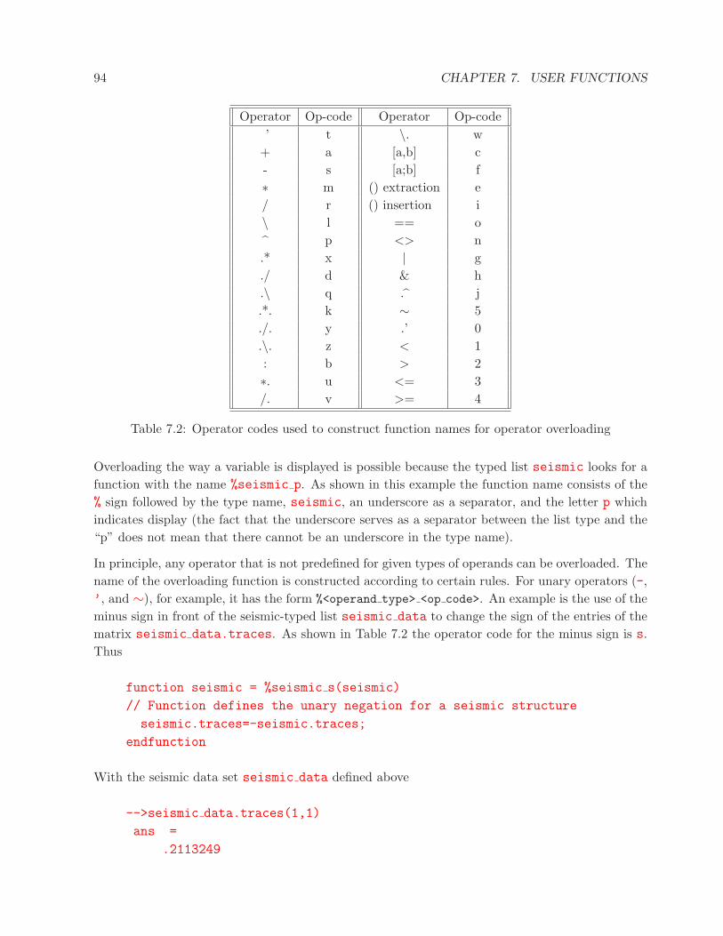
94 CHAPTER 7. USER FUNCTIONS
Operator Op-code Operator Op-code’ t \. w
+ a [a,b] c- s [a;b] f∗ m () extraction e/ r () insertion i\ l == o p <> n.* x | g./ d & h.\ q . j.*. k ∼ 5./. y .’ 0.\. z < 1: b > 2∗. u <= 3/. v >= 4
Table 7.2: Operator codes used to construct function names for operator overloading
Overloading the way a variable is displayed is possible because the typed list seismic looks for afunction with the name %seismic p. As shown in this example the function name consists of the% sign followed by the type name, seismic, an underscore as a separator, and the letter p whichindicates display (the fact that the underscore serves as a separator between the list type and the“p” does not mean that there cannot be an underscore in the type name).
In principle, any operator that is not predefined for given types of operands can be overloaded. Thename of the overloading function is constructed according to certain rules. For unary operators (-,’, and ∼), for example, it has the form %<operand type> <op code>. An example is the use of theminus sign in front of the seismic-typed list seismic data to change the sign of the entries of thematrix seismic data.traces. As shown in Table 7.2 the operator code for the minus sign is s.Thus
function seismic = %seismic s(seismic)
// Function defines the unary negation for a seismic structure
seismic.traces=-seismic.traces;
endfunction
With the seismic data set seismic data defined above
-->seismic data.traces(1,1)
ans =
.2113249
7.3. FUNCTIONS FOR OPERATOR OVERLOADING 95
-->seismic data = -seismic data;
-->seismic data.traces(1,1)
ans =
- .2113249
The function name for overloading binary operators has the form%<first operand type> <op code> <second operand type>. In this definition <operand type>
is code for the type of variable the operator of type <op code> is operating on. Operand types,i.e. codes for the various Scilab variables, are listed in the rightmost column of Table 4.1 on page19. An example is the following function which defines the operation of adding a scalar to a seismicdata set.
function seismic = %seismic a s(seismic,c)
// Function adds a constant to the matrix "seismic traces"
seismic.traces = seismic.traces + c;
endfunction
Here <first operand type> is seismic and the <second operand type> is s. A quick look atTable 4.1 shows that s is the operand type of a constant. As shown in Table 7.2, a is the operatorcode for + (addition). Thus
-->seismic data.traces(1,1)
ans =
.2113249
-->seismic data = seismic data + 1;
-->seismic data.traces(1,1)
ans =
1.2113249
It is important to note that overloading the operator + via %seismic a s(seismic,c) is onlydefined for this specific sequence of operands. The expression 1 + seismic data causes an errormessage as does, for example, seismic data - 1; but seismic data + (-1) works.
Some primitive functions can also be overloaded if they are not defined for the data type. In thiscase the function name has the form %<type of argument> <function name>. The function belowtakes the absolute value of the traces of a seismic data set.
function seismic = %seismic abs(seismic)
// Function takes the absolute value of the entries of the
// matrix ‘‘seismic.traces’’
seismic.traces = abs(seismic.traces);
endfunction
96 CHAPTER 7. USER FUNCTIONS
Thus, for the seismic data set seismic data defined above,
-->seismic data.traces(1,1)
ans =
.2113249
-->seismic data = abs(-seismic data);
-->seismic data.traces(1,1)
ans =
.2113249
Extraction of object elements can be overloaded by means of a function the name of which has theform %<operand type> e(i1,...,in,operand). A somewhat simplified example is
function seis = %seismic e(i,j,seis)
// Function extracts rows i and columns j of the ...
// matrix "seis.traces"; i and j can be vectors
seis.traces = seis.traces(i,j);
seis.last = seis.first+(i($)-1)*seis.step;
seis.first = seis.first+(i(1)-1)*seis.step;
endfunction
which outputs a seismic data set where seis.matrix consists only of the elements i,j of the inputmatrix. An example is
-->seismic data.traces(5,10)
ans =
.1853351
-->temp = seismic data(5,10)
temp =
LIST OF TYPE "seismic"
first: 16
last: 16
step: 4
traces: .1853351
units: ms
It is important to keep in mind that typed lists have extraction (component extraction) defined forone index. Hence, extraction with one index cannot be overloaded, and
7.4. TRANSLATION OF MATLAB-4 M-FILES TO SCILAB FORMAT 97
-->seismic data(4)
ans =
4.
produces the fourth element of typed list seismic, step, which is 4 (remember that the firstelement is the string vector [’seismic’,’first’,’last’,’step,’traces’].
It is also possible to extract data object elements to more than one output objects. Furthermore,the insertion syntax and row and column concatenation can also be overloaded.
7.4 Translation of Matlab-4 m-files to Scilab Format
A function, mfile2sci, is available to translate Matlab m-files to Scilab. This function is still beingworked on by someone in the Scilab team (it is likely to be a never-ending task) but the existingversion greatly simplifies this kind of conversion. It relieves the user of a lot of drudgery andlets him concentrate on the thornier problems: instances where Matlab and Scilab functions maydiffer slightly, possibly depending on parameters in the argument list, where functions unknown tomfile2sci are used, etc. mfile2sci allows individual files or whole directories to be converted.In the process it creates a *.sci file, a “compiled” *.bin file, and a *.cat file (help file). The latteris generated from the comment lines at the beginning of the m-file, those lines that are also usedby Matlab’s help facility. An example is
mfile2sci(’D:\MyScilab\Geophysics\read las file.m’, ...
’D:\MyScilab\Geophysics’)
Details about the conversion can be found in file SCIDIR\macros\m2sci\README; SCIDIR denotesthe Scilab root directory (in Windows something like C:\Program Files\Scilab).
Another useful function is translatepaths which translates all Matlab m-files in a set of direc-tories to Scilab. It uses mfile2sci to translate the individual files.

Chapter 8
Function Libraries
This is a topic that has no analog in Matlab. Libraries are collections of compiled functions thatcan be loaded automatically upon startup or that can be loaded on demand. There are severalways of creating libraries; the one described in the following appears to be the least painful.
Say, C:\MyScilab is a directory/folder with two Scilab functions (file extension .sci).
-->unix w(’ls C:\MyScilab’)lower.sci
upper.sci
Then a possible procedure to create a library is as follows;
-->genlib(’Mylib’,’C:\MyScilab’)Function genlib compiles every Scilab function (file with extension .sci) in directory C:\MyScilaband saves it in a file with the same root but extension .bin. It also creates the text file names withthe names of all functions, and a library file lib. Hence, directory C:\MyScilab now contains thefollowing files
-->unix w(’ls C:\MyScilab’)lib
lower.bin
lower.sci
names
upper.bin
upper.sci
In addition the variable Mylib of type library (type 14) is created in the workspace and all Scilabfunctions in C:\MyScilab are now available for use.
It is important to note that this does not create help files. This has to be done separately. Fur-thermore, the statement
98
99
load(’D:\MyScilab\lib’);
in the startup file .scilab will load the library Mylib every time Scilab is started. Note that thelibrary name Mylib is not mentioned in the load statement. Nevertheless, the variable Mylib oftype library shows up in the workspace (the library lib “knows” that its name in the workspaceis Mylib).
There are a few things to keep in mind with regard to loading libraries. This is illustrated in thefollowing.
-->clear // Remove all unprotected variables from the workspace
-->who // Show all variables
your variables are...
%helps scicos pal MSDOS home PWD TMPDIR
plotlib percentlib soundlib xdesslib utillib tdcslib
siglib s2flib roblib optlib metalib elemlib commlib
polylib autolib armalib alglib intlib mtlblib WSCI
SCI %F %T %z %s %nan %inf
$ %t %f %eps %io %i %e
using 5517 elements out of 10000000. and 41
variables out of 1791
-->lc = lower(’ABC’)
!--error 4
undefined variable : lower
Since all unprotected variables have been removed the function lower is not available. To get itback one can load the library Mylib, and the command who shows that the variable Mylib is nowin the workspace.
-->load(’D:\MyScilab\lib’) // Load library containing function lower
-->who
your variables are...
Mylib %helps scicos pal MSDOS home
PWD TMPDIR plotlib percentlib soundlib
xdesslib
utillib tdcslib siglib s2flib roblib optlib metalib
elemlib commlib polylib autolib armalib alglib intlib
mtlblib WSCI SCI %F %T %z %s
%nan %inf $ %t %f %eps %io
%i %e
100 CHAPTER 8. FUNCTION LIBRARIES
using 5553 elements out of 10000000.
and 42 variables out of 1791
It is important to note, however, that loading a library does not mean that the functions in it areloaded into the workspace; they are only marked as available to be loaded when called. Hence,lower is not listed yet. Nevertheless, we can now execute the function lower and expect it to beloaded.
-->lc = lower(’ABC’)
lc =
abc
-->who
your variables are...
lc lower Mylib %helps scicos pal
MSDOS home PWD TMPDIR plotlib percentlib
soundlib xdesslib utillib tdcslib siglib s2flib roblib
optlib metalib elemlib commlib polylib autolib armalib
alglib intlib mtlblib WSCI SCI %F %T
%z %s %nan %inf $ %t %f
%eps %io %i %e
using 5650 elements out of 10000000.
and 44 variables out of 1791
This statement adds two more variables to the workspace: the string variable lc and the functionlower.
Functions in libraries are actually loaded only if they are still undefined and their name is encoun-tered during execution! Thus a potential problem exists if the library function name is the sameas that of a built-in function or an already defined user function. In this case it would not beloaded. A related problem would come up if one found a bug in, say, lower, fixed it, and rebuiltand reloaded the library. If lower is executed again one would not get the corrected version in therebuild library Mylib but rather the one in variable lower. Hence, in order to get the correctedversion it is not only necessary to rebuild and load the new library but also to remove the variablelower from the workspace; in other words: it is necessary to execute the command
-->clear lower
An alternative is to bring the corrected version of lower into the workspace via
-->getf(’C:\MyScilab\lower.sci’)
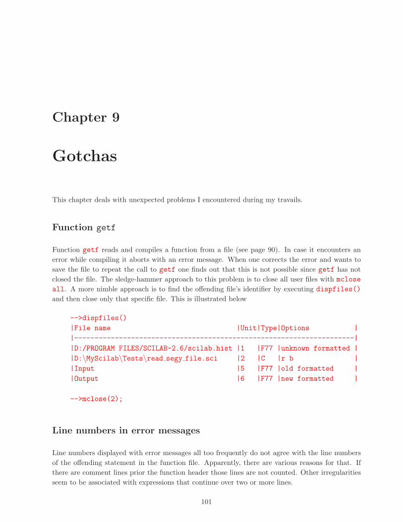
Chapter 9
Gotchas
This chapter deals with unexpected problems I encountered during my travails.
Function getf
Function getf reads and compiles a function from a file (see page 90). In case it encounters anerror while compiling it aborts with an error message. When one corrects the error and wants tosave the file to repeat the call to getf one finds out that this is not possible since getf has notclosed the file. The sledge-hammer approach to this problem is to close all user files with mclose
all. A more nimble approach is to find the offending file’s identifier by executing dispfiles()
and then close only that specific file. This is illustrated below
-->dispfiles()
|File name |Unit|Type|Options |
|---------------------------------------------------------------------|
|D:/PROGRAM FILES/SCILAB-2.6/scilab.hist |1 |F77 |unknown formatted |
|D:\MyScilab\Tests\read segy file.sci |2 |C |r b |
|Input |5 |F77 |old formatted |
|Output |6 |F77 |new formatted |
-->mclose(2);
Line numbers in error messages
Line numbers displayed with error messages all too frequently do not agree with the line numbersof the offending statement in the function file. Apparently, there are various reasons for that. Ifthere are comment lines prior the function header those lines are not counted. Other irregularitiesseem to be associated with expressions that continue over two or more lines.
101
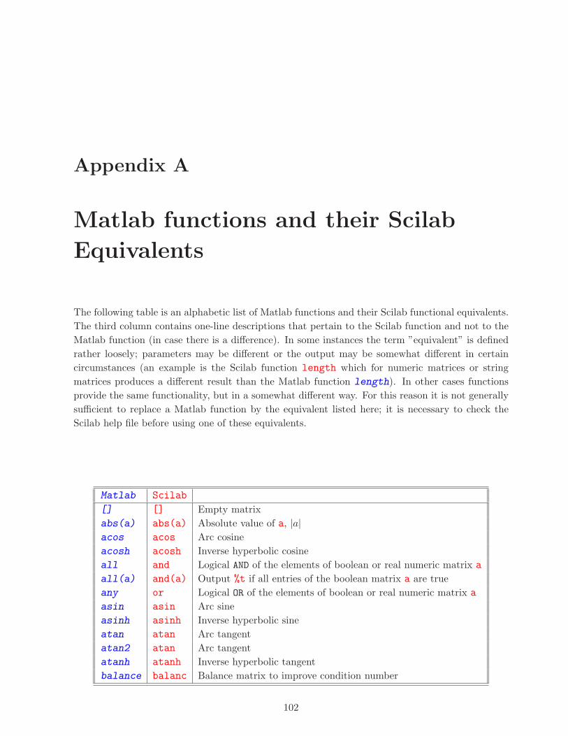
Appendix A
Matlab functions and their Scilab
Equivalents
The following table is an alphabetic list of Matlab functions and their Scilab functional equivalents.The third column contains one-line descriptions that pertain to the Scilab function and not to theMatlab function (in case there is a difference). In some instances the term ”equivalent” is definedrather loosely; parameters may be different or the output may be somewhat different in certaincircumstances (an example is the Scilab function length which for numeric matrices or stringmatrices produces a different result than the Matlab function length). In other cases functionsprovide the same functionality, but in a somewhat different way. For this reason it is not generallysufficient to replace a Matlab function by the equivalent listed here; it is necessary to check theScilab help file before using one of these equivalents.
Matlab Scilab
[] [] Empty matrixabs(a) abs(a) Absolute value of a, |a|acos acos Arc cosineacosh acosh Inverse hyperbolic cosineall and Logical AND of the elements of boolean or real numeric matrix a
all(a) and(a) Output %t if all entries of the boolean matrix a are trueany or Logical OR of the elements of boolean or real numeric matrix a
asin asin Arc sineasinh asinh Inverse hyperbolic sineatan atan Arc tangentatan2 atan Arc tangentatanh atanh Inverse hyperbolic tangentbalance balanc Balance matrix to improve condition number
102
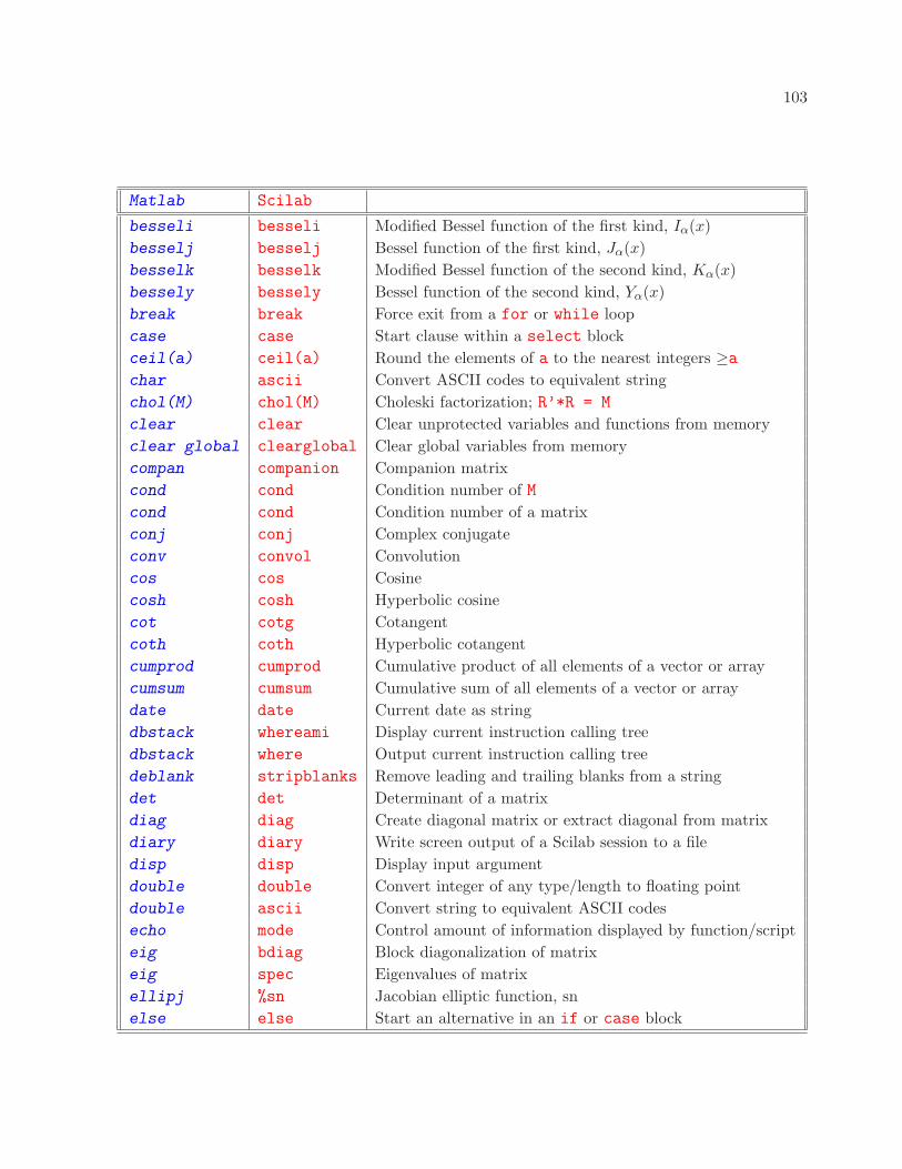
103
Matlab Scilab
besseli besseli Modified Bessel function of the first kind, Iα(x)besselj besselj Bessel function of the first kind, Jα(x)besselk besselk Modified Bessel function of the second kind, Kα(x)bessely bessely Bessel function of the second kind, Yα(x)break break Force exit from a for or while loopcase case Start clause within a select blockceil(a) ceil(a) Round the elements of a to the nearest integers ≥achar ascii Convert ASCII codes to equivalent stringchol(M) chol(M) Choleski factorization; R’*R = M
clear clear Clear unprotected variables and functions from memoryclear global clearglobal Clear global variables from memorycompan companion Companion matrixcond cond Condition number of Mcond cond Condition number of a matrixconj conj Complex conjugateconv convol Convolutioncos cos Cosinecosh cosh Hyperbolic cosinecot cotg Cotangentcoth coth Hyperbolic cotangentcumprod cumprod Cumulative product of all elements of a vector or arraycumsum cumsum Cumulative sum of all elements of a vector or arraydate date Current date as stringdbstack whereami Display current instruction calling treedbstack where Output current instruction calling treedeblank stripblanks Remove leading and trailing blanks from a stringdet det Determinant of a matrixdiag diag Create diagonal matrix or extract diagonal from matrixdiary diary Write screen output of a Scilab session to a filedisp disp Display input argumentdouble double Convert integer of any type/length to floating pointdouble ascii Convert string to equivalent ASCII codesecho mode Control amount of information displayed by function/scripteig bdiag Block diagonalization of matrixeig spec Eigenvalues of matrixellipj %sn Jacobian elliptic function, snelse else Start an alternative in an if or case block

104 APPENDIX A. MATLAB FUNCTIONS AND THEIR SCILAB EQUIVALENTS
Matlab Scilab
elseif elseif Start a conditional alternative in an if blockend [loop] end Terminate for, if, select, or while clauseend [matrix] $ Index of last element of matrix or (row/column) vectorerf erf Error function, erf(x) = 2/
√π
∫ x0 exp(−t2)dt
erfc erfc Complementary error function, erfc(x) = 2/√
π∫∞x exp(−t2)dt
erfcx erfcx Scaled complementary error function, erfcx(x) = exp(x2)erfc(x)error error Print error message and aborteval execstr Evaluate string vector with Scilab expressions or statementsexist(a) exists(a) Test if variable a existsexp exp Exponential functionexpm expm Matrix xponential functioneye eye Identity matrix (or its generalization)fclose mclose Close (all) open file(s)fft fft Forward and inverse Fast Fourier Transformfft2 fft Forward and inverse Fast Fourier Transformfigure xset Set defaults for current graphics windowfind spget Retrieve entries of a sparse matrixfind(a) find(a) Find the indices for which boolean matrix a is truefindstr strindex Find starting position(s) of a string in an other stringfix(a) fix(a) Rounds the elements of a to the nearest integers towards zerofloor(a) floor(a) Rounds the elements of a to the nearest integers ≥ a
fopen mopen Open a filefor for Start a loop with a generally known number of repetitionsfprintf fprintf Write formatted data to file (like C-language fprintf function)full full Convert sparse to full matrixfunction function Identify header of function definitiongamma gamma Gamma function, Γ(x) =
∫∞0 tx−1 exp(−t)dt
gammaln gammaln Logarithm of the Gamma function, ln(Γ(x))getfield getfield Get a data object from a listglobal global Define variables as globalhelp help On-line helphess(M) hess(M) Hessenberg form of Mif if Start a conditionally executed block of statementsifft fft Forward and inverse Fast Fourier Transformifft2 fft Forward and inverse Fast Fourier Transformimag imag Imaginary part of a matrixinput input Prompt for user (keyboard) input

105
Matlab Scilab
int16(a) int16(a) Convert a to 16-bit signed integerint32(a) int32(a) Convert a to 32-bit signed integerint8(a) int8(a) Convert a to 8-bit signed integerintersect intersect Returns elements common to two vectorsinv(M) inv(M) Inverse of matrix M
isempty(a) a==[] Check if variable a is emptyisglobal(a) isglobal(a) Test if a is a global variableisinf(a) isinf(a) Test if a is infiniteisnan(a) isnan(a) Output boolean vector with entries %t where a is %nanisreal(a) isreal(a) Test if a is real (or if its imaginary part is “small”)keyboard pause Interrupt execution of function or scriptlength length Length of list; product of no. of rows and columns of matrixlinspace linspace Create vector with linearly spaced elementslog log Natural logarithmlog10 log10 Base-10 logarithmlog2 log2 Base-2 logarithmlogm logm Matrix natural logarithmlogspace logspace Create vector with logarithmically spaced elementslookfor apropos Keyword search for a functionlower convstr Convert string to lower or upper casemax maxi Maximum of all elements of a vector or arraymax max Maximum of all elements of a vector or arraymean mean Mean of all elements of a vector or arraymedian median Median of all elements of a vector or arraymin min Minimum of all elements of a vector or arraymin mini Minimum of all elements of a vector or arraymod(a,b) pmodulo(a,b) a-b.*floor(a./b) if b∼=0; remainder of a divided by b
more lines Specify number of lines to display and columns/linenargin argn Number of input/output arguments of a functionnargout argn Number of imput/output arguments of a functionnnz nnz Number of nonzero elements of a sparse matrixnorm(M) norm(M) Norm of M (matrix or vector)null(M) kernel(M) Nullspace of Mnum2str string Convert numbers to stringsones ones Matrix of onesorth(M) orth(M) Orthogonal basis for the range of Mpause halt Stop execution and wait for a key press
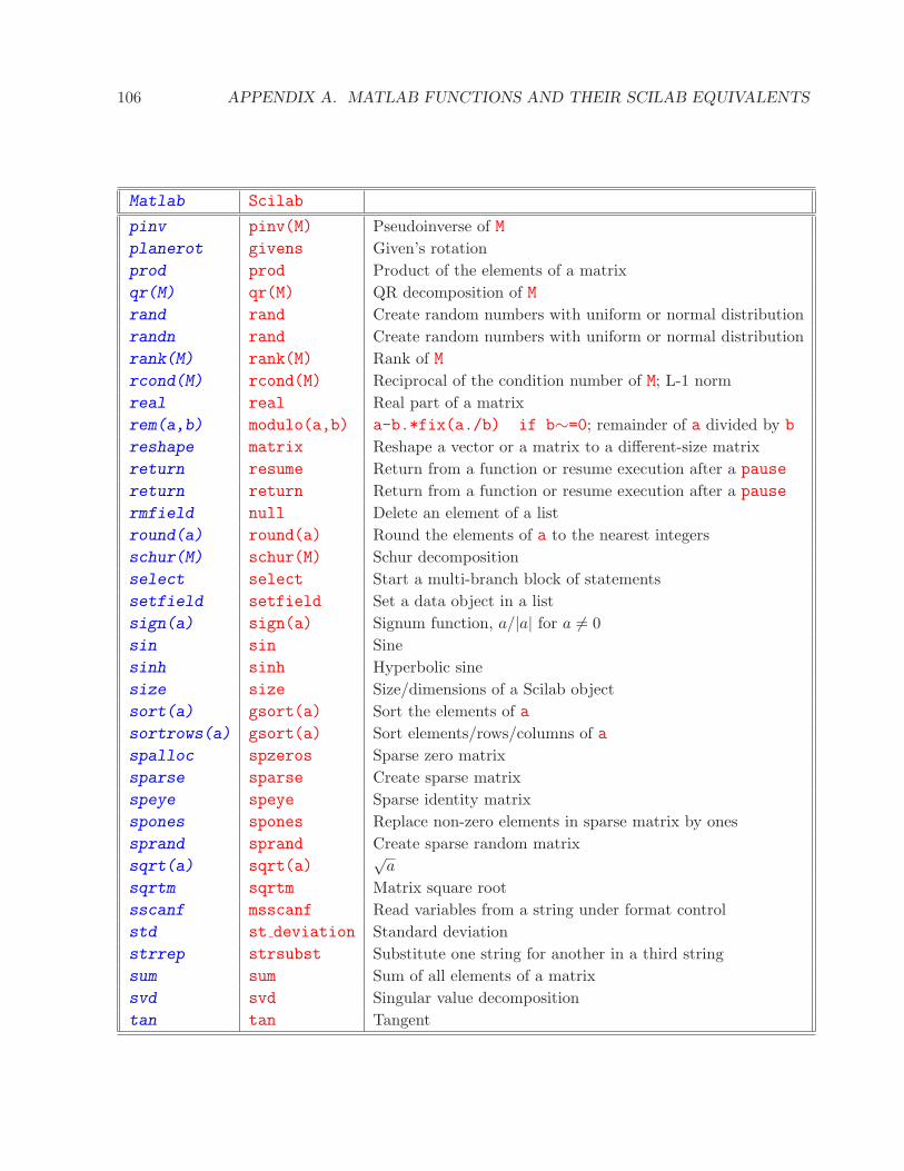
106 APPENDIX A. MATLAB FUNCTIONS AND THEIR SCILAB EQUIVALENTS
Matlab Scilab
pinv pinv(M) Pseudoinverse of Mplanerot givens Given’s rotationprod prod Product of the elements of a matrixqr(M) qr(M) QR decomposition of Mrand rand Create random numbers with uniform or normal distributionrandn rand Create random numbers with uniform or normal distributionrank(M) rank(M) Rank of Mrcond(M) rcond(M) Reciprocal of the condition number of M; L-1 normreal real Real part of a matrixrem(a,b) modulo(a,b) a-b.*fix(a./b) if b∼=0; remainder of a divided by b
reshape matrix Reshape a vector or a matrix to a different-size matrixreturn resume Return from a function or resume execution after a pause
return return Return from a function or resume execution after a pause
rmfield null Delete an element of a listround(a) round(a) Round the elements of a to the nearest integersschur(M) schur(M) Schur decompositionselect select Start a multi-branch block of statementssetfield setfield Set a data object in a listsign(a) sign(a) Signum function, a/|a| for a 6= 0sin sin Sinesinh sinh Hyperbolic sinesize size Size/dimensions of a Scilab objectsort(a) gsort(a) Sort the elements of asortrows(a) gsort(a) Sort elements/rows/columns of aspalloc spzeros Sparse zero matrixsparse sparse Create sparse matrixspeye speye Sparse identity matrixspones spones Replace non-zero elements in sparse matrix by onessprand sprand Create sparse random matrixsqrt(a) sqrt(a)
√a
sqrtm sqrtm Matrix square rootsscanf msscanf Read variables from a string under format controlstd st deviation Standard deviationstrrep strsubst Substitute one string for another in a third stringsum sum Sum of all elements of a matrixsvd svd Singular value decompositiontan tan Tangent

107
Matlab Scilab
tanh tanh Hyperbolic tangenttic timer() Ouputs time elapsed since the call to timer()
toc timer Ouputs time elapsed since the preceding call to timer()
toeplitz toeplitz Toeplitz matrixtrace trace Trace (sum of diagonal elements) of a matrixtril tril Extract lower-triangular part of a matrixtriu triu Extract upper-triangular part of a matrixtry errcatch Trap erroruigetfile xgetfile Open dialog box for file selectionuint16(a) uint16(a) Convert a to 16-bit unsigned integeruint32(a) uint32(a) Convert a to 32-bit unsigned integeruint8(a) uint8(a) Convert a to 8-bit unsigned integerunion union(a,b) Extract the unique common elements of a and b
unique(a) unique(a) Return the unique elements of a in ascending orderunix unix w Execute Unix/DOS command; output to Scilab windowupper convstr Convert string to lower or upper casevarargin varargin Variable number of input arguments for a functionvarargout varargout Variable number of output arguments for a functionversion getversion Display version of Scilabwarning warning Print warning messagewhich whereis Display name of library containing functionwhile while Start repeated execution of a block while a condition is satisfiedwho who Displays/outputs names of current variableswhos whos Displays/outputs names and specifics of current variableszeros zeros Matrix of zeros
Index
argumentsnamed, 55variable-length list of, 56, 87
ASCII codes, 27
boolean operators, 35boolean variables, 35
cell array, 6, 25, 26, 39–42character string, see stringcommand-style syntax, 15, 54, 81comments, 7complex number, 21constants, built-in, 10continuation of a statement, 8convolution, 64, 103copy, 5
date, 16directory
private, see private directoryDOS, see MS-DOS
end of file, 67error trapping, 12, 14, 15, 32, 33, 72, 78, 82
Fast Fourier Transform, 64–65, 104FFT, see Fast Fourier Transformfile, 66–75
opening, closing, 66flow control, 12font, 4format
loose, 2tight, 2
functionas argument, 89as variable, 89
inline, 91, 92library, 90loading, 90overloading, 95private, see private functionScilab, 54–77user, 84–97
help, 5, 6
integer, 74interrupt, see pause
Kroneckerproduct, 8division, 8
last elementof vector or matrix, 22, 30
LATEX, 76length
list, 42numeric matrix, 15string, 25, 26, 30
library, 98–100lines displayed, 4list, 39
matrix-like typed, 49–50ordinary, 39–43polynomials, 50–53typed, 6, 42–49, 96
Matlabm-file conversion, 97emulation, 6
Matlab-mode, 24matrix, 21, 22, 24, 107
companion, 24, 103
108

INDEX 109
empty, 24, 102Frank, 24Hilbert, 24identity, 24, 104of ones, 24, 105of zeros, 24, 107polynomial, see polynomial matrix, 51random, 24, 106rational, 51reshape a, 106sparse, 62sparse identity, 62, 106sparse random, 62, 106Toeplitz, 24, 107
MS-DOS, 77
operatorbinary, 95code, 94, 95overloading, 19, 44, 50, 92–97unary, 94
overloadingoperator, see operator, overloadingvariable display, see variable, display over-
loading
paging, see lines displayedpaste, 5path, 81polynomial, 50–53, 76
division, 51matrix, 51
private directory, 91private function, 91program
exit, 5interrupt, 5, 15quit, 5resume, 5
Scilabsyntax, 7, 8
script, 78–83search path, 32, 81
sizelist, 42string, 25–27
sorting, 58–59startup file, 4, 99string
concatenation, 27, 92extraction, 28
structure, 1, 39, 44–47
termination script, 5time, 16tuple assignment, 9, 41type name, 43, 44, 92, 94type of variable, 19, 20
boolean matrix, 19boolean sparse matrix, 19compiled function, 19constant, 19function library, 19implied-size vector, 19, 22integer, 20list, 19Matlab sparse matrix, 19matrix-like typed list, 19pointer, 19polynomial matrix, 19rational, 38, 51, 53sparse matrix, 19string, 19typed list, 19un-compiled function, 19
typed list, see list, typed
UNIX, 77
variableconversion into an expression, 31display overloading, 93, 94global, 16, 87, 88, 104name, 7, 8, 91type, see type, variable
working directory, 78

110 INDEX
workspace, 1, 5, 15–17, 33, 73, 78, 86, 88, 89,98–100
Index of Scilab Functionsand Variables
[], 24, 102$, 16, 22, 29, 30, 46, 104%asn, 62%io, 77%k, 62%sn, 62, 103
a==[], 105abort, 5abs, 57, 102acos, 60, 102acosh, 60, 102acoshm, 61acosm, 61amell, 62and, 37, 38, 102apropos, 5, 6, 16, 105argn, 85, 88, 105ascii, 26, 27, 29, 30, 103asin, 60, 102asinh, 60, 102asinhm, 61atan, 59, 60, 102atanh, 60, 102atanhm, 61auread, 68auwrite, 69
balanc, 63, 102bandwr, 62bdiag, 63, 103besseli, 62, 103besselj, 62, 103besselk, 62, 103bessely, 62, 103bezout, 51blanks, 29bool2s, 38, 57
break, 12, 103
case, 12, 103ceil, 57, 103chdir, 81chfact, 62chol, 63, 103chsolve, 62clean, 51, 57, 61clear, 16, 99, 100, 103clearglobal, 16, 103cmndred, 51coeff, 51coffg, 51colcomp, 63colcompr, 51companion, 24, 103cond, 63, 103conj, 57, 103convol, 64, 103convstr, 26, 89, 105, 107cos, 60, 103cosh, 60, 103coshm, 61cosm, 61cotg, 60, 103coth, 60, 103cumprod, 57, 103cumsum, 57, 103
date, 16, 26, 103deff, 91, 92degree, 51delip, 62denom, 51derivat, 51det, 51, 63, 103determ, 51detr, 51diag, 24, 103diary, 69, 76, 103diophant, 51disp, 16, 18, 69, 75, 103dispfiles, 67, 101
INDEX 111
dlgamma, 62double, 22, 103
edit, 90else, 12, 103elseif, 12, 104emptystr, 26, 29, 30end, 12, 104endfunction, 85erf, 62, 104erfc, 62, 104erfcx, 62, 104errcatch, 12, 14, 15, 107errclear, 14, 15error, 85, 104eval, 32evstr, 32–34excel2sci, 68exec, 79, 81execstr, 32, 78, 82, 104exists, 15, 36, 38, 104exit, 5exp, 60, 104expm, 61, 104eye, 24, 104
factors, 51fft, 64, 104file, 66, 67, 71, 72, 82, 83fileinfo, 67find, 38, 104fix, 57, 104floor, 57, 104for, 12, 104fprintf, 69, 104fprintfMat, 69fscanf, 68fscanfMat, 68full, 62, 104fullrf, 63fullrfk, 63function, 85, 104
gamma, 62, 104
gammaln, 62, 104gcd, 51genlib, 90, 98getd, 90getdate, 16getf, 90, 100, 101getfield, 40, 104getio, 67getversion, 76, 107givens, 63, 106global, 16, 81, 86–88, 104grand, 24grep, 26, 30gsort, 26, 57–59, 106
halt, 15, 16, 85, 105help, 5, 6, 16, 104hermit, 51hess, 63, 104horner, 51host, 76, 77householder, 63hrmt, 51
iconvert, 22if, 12, 13, 104imag, 57, 104input, 68, 75, 104int16, 22, 105int32, 22, 105int8, 22, 23, 105intersect, 26, 57, 105inttype, 16, 20inv, 51, 63, 105invr, 51isdef, 36, 38iserror, 14, 38isglobal, 38, 105isinf, 38, 105isletter, 27ismember, 39isnan, 38, 105isreal, 38, 105

112 INDEX
kernel, 63, 105
lcm, 51lcmdiag, 51ldiv, 51length, 6, 26, 40, 42, 105lex sort, 57lines, 76, 105linsolve, 63linspace, 57, 105list, 19, 39, 40load, 68, 73, 74, 90, 99loadwave, 68log, 60, 105log10, 60, 105log2, 60, 105logm, 61, 105logspace, 57, 105lstcat, 40lufact, 62luget, 62lusolve, 62
matrix, 70, 106max, 56, 57, 105maxi, 57, 105mclearerr, 67mclose, 66, 67, 69, 101, 104mean, 57, 105median, 57, 105meof, 67mfft, 64mfprintf, 69mfscanf, 68mget, 68, 74, 75mgeti, 68, 74mgetl, 67–70mgetstr, 68min, 57, 105mini, 57, 105mlist, 19, 39, 40, 49mode, 78–81, 85, 103modulo, 57, 106mopen, 66–68, 71, 73, 75, 104
mprintf, 69mput, 69, 74mputl, 67, 69–71mputstr, 69mscanf, 68MSDOS, 38, 77mseek, 67msprintf, 26msscanf, 26, 31, 106mtell, 67mtlb cell, 6mtlb diff, 6mtlb load, 68mtlb mode, 24, 38mtlb save, 69
newest, 67nnz, 62, 105norm, 63, 105null, 40, 41, 106
ones, 24, 36, 105or, 37, 38, 102orth, 63, 105otherwise, 12
part, 26, 29, 82pause, 5, 15–17, 85, 88, 105pdiv, 51pinv, 63, 106pmodulo, 57, 105pol2str, 26, 51pol2tex, 76polar, 63poly, 50print, 69printf, 69prod, 57, 106
qr, 63, 106quit, 5
rand, 24, 106range, 63rank, 63, 106
INDEX 113
rcond, 63, 106read, 68, 70, 71read4b, 68readb, 68readc , 68real, 57, 106reshape, 70residu, 51resume, 5, 18, 85, 88, 106return, 5, 16–18, 82, 85, 88, 106roots, 51round, 57, 106rowcompr, 51
save, 68, 73, 74savewave, 69scanf conversion, 31schur, 63, 106sci2exp, 31sci2expr, 26select, 12, 106setfield, 40, 106sfact, 51sign, 57, 106simp, 51simp mode, 38, 51, 52sin, 60, 106sinh, 60, 106sinhm, 61sinm, 61size, 25, 26, 40, 42, 106spaninter, 63spanplus, 63sparse, 62, 106spchol, 62spec, 63, 103speye, 62, 106spget, 62, 104spones, 62, 106sprand, 62, 106spzeros, 62, 106sqrt, 57, 106sqrtm, 61, 106st deviation, 57, 106
stacksize, 76strcat, 26, 28strindex, 26, 30, 104string, 26, 105stripblanks, 26, 29, 103strsubst, 26, 106sum, 57, 106sva, 63svd, 63, 106sylm, 24, 51
tan, 60, 106tanh, 60, 107tanhm, 61tanm, 61testmatrix, 24texprint, 76timer, 16, 76, 107tlist, 19, 39, 40, 43, 46toeplitz, 24, 107trace, 63, 107tril, 107triu, 107type, 16, 19, 20, 91, 92typename, 20typeof, 16, 19, 20, 23, 31, 89, 92
uint16, 22, 107uint32, 22, 107uint8, 20, 22, 107union, 26, 57, 107unique, 26, 57, 107unix, 76unix g, 76, 77unix s, 76unix w, 76, 98, 107unix x, 76
varargin, 56, 85, 107varargout, 85, 107
warning, 85, 107wavread, 68wavwrite, 69where, 85, 103

114 INDEX
whereami, 85, 103whereis, 16, 85, 107while, 12, 107who, 16, 20, 99, 107whos, 16, 20, 107writb, 69write, 69–73, 77write4b, 69
xgetfile, 67, 75, 107xset, 104
zeros, 24, 36, 107
Index of Matlab Functionsand Variables
[], 102
abs, 102acos, 102acosh, 102all, 37, 102any, 37, 38, 102asin, 102asinh, 102atan, 59, 102atan2, 59, 102atanh, 102
balance, 102besseli, 103besselj, 103besselk, 103bessely, 103blanks, 29break, 12, 103
case, 12, 103catch, 12, 14ceil, 103cell, 6, 30char, 27, 103chol, 103clear, 103
clear global, 103compan, 103complex, 21cond, 103conj, 103conv, 103cos, 103cosh, 103cot, 103coth, 103cumprod, 103cumsum, 103
date, 103dbstack, 103deal, 9deblank, 29, 103det, 103diag, 103diary, 76, 103diff, 6disp, 103double, 27, 103
echo, 103eig, 103ellipj, 103else, 12, 103elseif, 12, 104end, 22end [loop], 12, 104end [matrix], 46, 104erf, 104erfc, 104erfcx, 104error, 104eval, 32, 104evalin, 33exist, 15, 104exp, 104expm, 104eye, 104
fclose, 104

INDEX 115
feval, 89fft, 64, 104fft2, 64, 104figure, 104find, 104findstr, 104finish, 5fix, 104floor, 104fopen, 66, 75, 104for, 12, 104fprintf, 104full, 104function, 104funm, 61
gamma, 104gammaln, 104getfield, 104global, 104
help, 5, 104hess, 104
if, 12, 104ifft, 64, 104ifft2, 64, 104imag, 104input, 75, 104int16, 105int32, 105int8, 105intersect, 105inv, 105isa, 20iscell, 19ischar, 19isempty, 105isglobal, 105isinf, 105isletter, 27ismember, 31, 38isnan, 105isnumeric, 19
isreal, 105issparse, 19isstruct, 19
keyboard, 17, 88, 105
length, 105linspace, 105load, 74log, 105log10, 105log2, 105logical, 35, 36logm, 105logspace, 105lookfor, 5, 105lower, 105
max, 57, 105mean, 105median, 105min, 105mod, 105more, 105
nargin, 105nargout, 105nnz, 105norm, 105null, 105num2str, 105
ones, 105orth, 105otherwise, 12
pause, 105pinv, 106planerot, 106prod, 106
qr, 106
rand, 106randn, 106rank, 106
116 INDEX
rcond, 106real, 106rem, 106reshape, 106return, 106rmfield, 106roots, 52round, 106
save, 73schur, 106select, 106setfield, 106sign, 106sin, 106sinh, 106size, 26, 50, 106sort, 58, 106sortrows, 58, 106spalloc, 106sparse, 106speye, 106spones, 106sprand, 106sqrt, 106sqrtm, 106sscanf, 31, 106std, 106strrep, 106sum, 106svd, 106switch, 12
tan, 106tanh, 107tic, 107toc, 107toeplitz, 107trace, 107tril, 107triu, 107try, 12, 14, 107type, 53typeof, 50, 53
uigetfile, 75, 107uint16, 107uint32, 107uint8, 20, 107union, 107unique, 107unix, 107upper, 107
varargin, 107varargout, 107version, 107
warning, 107which, 107while, 12, 107who, 107whos, 107
zeros, 107


