An introduction to SPEX

E. CostantiniJ. Kaastra, J. de Plaa

SRON

Introducing SPEX

• SPEX is a fitting package for X-ray spectralanalysis

• Similar packages: XSPEC (Arnaud et al. 1996), ION (Netzer et al. 2002), PHASE (Krongold et al. 2003) ISIS (Houck & Denicola 2000)ISIS (Houck & Denicola 2000)

• SPEX is optimized for high-resolutionspectroscopy: – Most updated atomic data bases– Several multi-parameters absorption/emission

models � accurate analysis of narrow features produced by different astrophysical processes

Where to get SPEXwww.sron.nl/spex

SPEX Manualhttp://www.sron.nl/files/HEA/SPEX/manuals/manual.pdf

Quick-start documentshttp://www.sron.nl/files/HEA/SPEX/manuals/spex_intro.pdf

Downloading SPEX

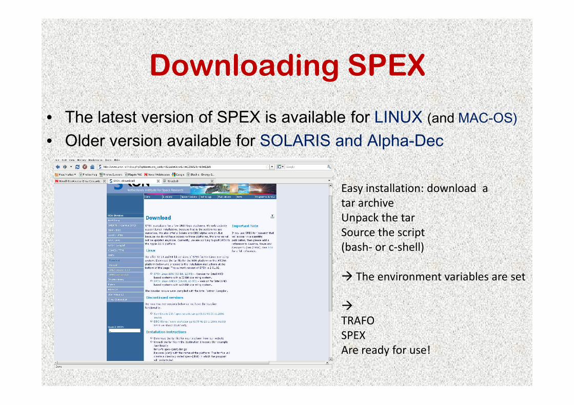
• The latest version of SPEX is available for LINUX (and MAC-OS)• Older version available for SOLARIS and Alpha-Dec

Easy installation: download a

tar archivetar archive

Unpack the tar

Source the script

(bash- or c-shell)

� The environment variables are set

�

TRAFO

SPEX

Are ready for use!

Step 1: using TRAFO

• TRAFO converts normal fits files intoSPEX format � trimmed, slimmer fits files.� new spectrum & response matrix

• Inputs:• Inputs:– Original spectrum (either binned or unbinned)– Background– Effective area– Response matrix

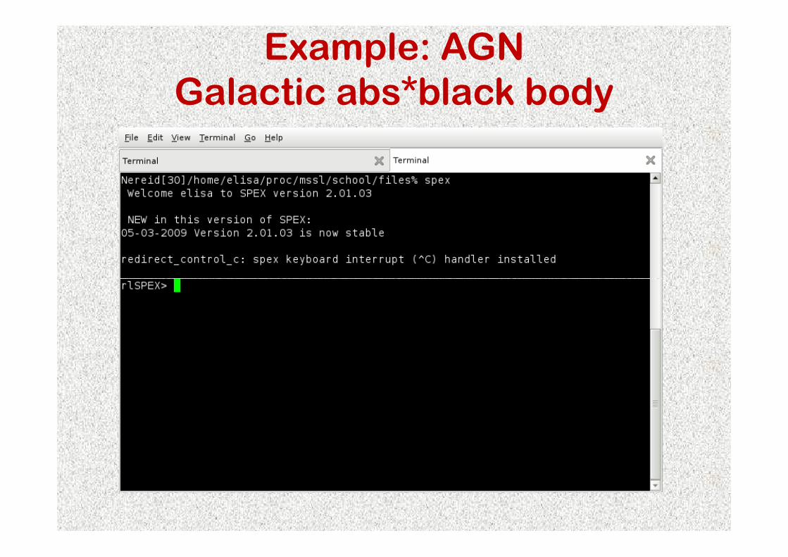
Example: AGN Galactic abs*black body

Example 1: fitting a black body

• Spectrum and response matrix are names bb.spo and bb.res

• Use the RGS band: 7:35 Angstrom

• Display the data in Angstrom

Save the plot:

SPEX> pl x lin

SPEX> pl y lin

SPEX> plot adump data_plot

� data_plot.qdp ready for post processing with pgplot

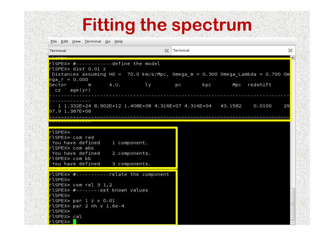
Fitting the spectrum

SPEX> Fit meth cs

SI units1erg=1e-7joule

Other useful types of plotting

• pl ty chi � residuals in terms of χ• pl uy rel � residuals relative to

the model

(data-model)/model

• pl ty model � plot of the current

model (ph m-2 s-1 Ang-1)

• pl ty data

• pl uy fa � cts s-1 m-2 Ang-1

• pl uy counts � number of

counts in a particular emission

feature

! A useful command file is in your

exercise kit: plot_rgs.pro

A “live” exampleFitting a

star spectrum: AU Microscopii

• AU Mic is a cool nearby star (9pc), with a thermal spectrum.

• Plasma at different temperatures (coming • Plasma at different temperatures (coming from different loops of the stellar corona) produces a wealth of lines in the RGS band.

� (Multiple) Collisionally ionized emissionmodel, CIE (see also E. Behar talk)

The RGS spectrum of AU Mic

CIE model parameters

Emission measure

CIE model parameters

Temperatures:

-- Electron Te

-- Ionic Ti � line thermal

broadening (dependence onbroadening (dependence on

the thermal velocity of the

ions and also on ion mass)

-- equilibrium Tb

�In CIE Tb/Te=1

Note: for non-equilibrium

use the NEI model.

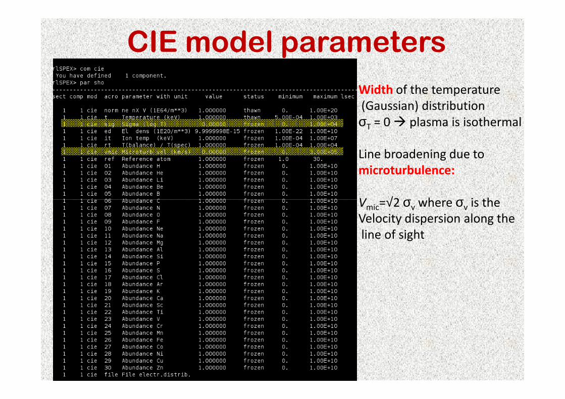
CIE model parameters

Width of the temperature

(Gaussian) distribution

σT = 0 � plasma is isothermal

Line broadening due to

microturbulence:

V =√2 σ where σ is the Vmic=√2 σv where σv is the

Velocity dispersion along the

line of sight

CIE model parameters

Electron density

Lines which are sensitive to

density will be adjusted in

normalization

CIE model parameters

Abundances

Deafult is set to solar

(Anders & Grevesse 89)

Change abundances:Change abundances:

SPEX> abu #a

Reference atom is H,

but for spectra with

strong lines (and weak

continuum) it’s

better to set the ref to

the strongest line (Fe)