Chapter 3

An Introduction to the

Approximation of Functions

In this Chapter, we will look at various ways of approximating functions from a given set of discrete

data points.

Interpolation is a method for constructing a function f(x) that fits a known set of data points

(xk, yk), i.e. a method for constructing new data points within the range of a discrete set of known

data points. There are various ways in which this can be done.

Given a sequence of n + 1 distinct numbers xk (called knots) with corresponding numbers yk we are

looking for a function f(x) such that

f(xk) = yk , k = 0, 1, ..., n

Each pair (xk, yk) is called a data point and f is called an interpolant for the data points.

3.1 Linear Interpolation

Given 2 discrete data points, for instance, (x0, y0) and (x1, y1), then it is possible to find a unique

straight line that fits these two points (Figure 3.1). The unique straight line can found by solving

the linear system

y0 = a1x0 + a0 ,

y1 = a1x1 + a0 .

39

Figure 3.1: Linear approximation (solid blue line) to the 2 data points (red), (x0, f(x0)) and

(x1, f(x1)), where f(x) is the function given by the purple dashed line.

This pair of simultaneous equations yields the result

a1 =y1 − y0

x1 − x0, and a0 = y0 −

(y1 − y0)

(x1 − x0)x0 .

So the interpolant for any x ∈ [x0, x1] is

p1(x) =(y1 − y0)

(x1 − x0)x + y0 −

(y1 − y0)

(x1 − x0)x0 ,

= y0 +(y1 − y0)

(x1 − x0)(x − x0) .

p1(x) is a first-degree polynomial and if y0 = f(x0) and y1 = f(x1) the equation above can easily

be re-arranged to give

p1(x) =(x0 − x1)

(x0 − x1)f(x0) +

(x − x0)

(x0 − x1)f(x0) −

(x − x0)

(x0 − x1)f(x1) .

=(x − x1)

(x0 − x1)f(x0) +

(x − x0)

(x1 − x0)f(x1) . (3.1)

3.2 Piecewise Linear Interpolation

Given a known set of n+1 discrete data points (xk, f(xk)) k = 0, 1, . . . , n that partition an interval

[a, b] into n sub-intervals [xk, xk+1] where

a = x0 < x1 < · · · < xn = b .

One of the easiest ways of approximating a given function f in C[a, b] is to form a function connecting

consecutive pairs of data points with straight line segments. This is known as piecewise linear

interpolation.

40

To find the unique straight line through any pair of consecutive data points (xk, f(xk)) and (xk+1, f(xk+1))

we generalise the formula in (3.1). So the interpolant for any x ∈ [xk, xk+1] is equal to

p1k(x) =(x − xk+1)

(xk − xk+1)f(xk) +

(x − xk)

(xk+1 − xk)f(xk+1) . (3.2)

By choosing n sufficiently large, i.e. ensuring the sub-intervals are sufficiently small, we can approx-

imate f as closely as we wish. In general, this interpolating function will be continuous but not

differentiable.

Example 3.1.1: Using the 4 data points given below and find the piecewise linear approximation to

these points.

k (xk, f(xk))

0 (0.0, 0.0)

1 (π/3, 0.8660)

2 (2π/3, 0.8660)

3 (π, 0.0)

By applying the formula (3.2) to each pair of adjacent data points we find the following 3 straight

lines:

P (x) =

0.8270x x ∈ [0.0, π/3]

0.0000x + 0.8660 x ∈ [π/3, 2π/3]

−0.8270x + 2.5981 x ∈ [2π/3, π]

This produces the plot given in Figure 3.2

Figure 3.2: (Example 3.1.1) Piecewise linear approximation (solid blue lines) to the 4 data points

(red). The purple dotted line is the function that created the data points.

41

3.2.1 The Linear Interpolation Error

An obvious question is how large is the error of our fit?

The error associated with a linear fit p1(x) between the points [a, b] to the function f(x) is

f(x) − p1(x) =1

2(x − a)(x − b)f ′′(ux) .

where ux lies somewhere in the interval [a, b].

Proof

First, we fix x ∈ [a, b] and use Taylor’s theorem to express the values of f(a) and f(b) in terms of

f(x), f ′(x), f ′′(ua) and f ′′(ub) where ua ∈ (a, x) and ub ∈ (x, b). This gives us

f(a) = f(x) + (a − x)f ′(x) +1

2(a − x)2f ′′(x) + . . . , (3.3)

f(b) = f(x) + (b − x)f ′(x) +1

2(b − x)2f ′′(x) + . . . , (3.4)

From (3.2) we rewrite p1(x) such that

p1(x) =x − b

a − bf(a) − x − a

a − bf(b) ,

and substituting in (3.3) for f(a) and (3.4) for f(b) gives

p1(x) =(x − b) − (x − a)

a − bf(x) +

(x − b)(a − x) − (x − a)(b − x)

a − bf ′(x) +

+1

2

((x − b)(a − x)2 − (x − a)(b − x)2

a − b

)

f ′′(x) + . . . ,

= f(x) +1

2

((x − b)(a − x)2 − (x − a)(b − x)2

a − b

)

f ′′(x) + . . . .

However, note that

((x − b)(a − x)2 − (x − a)(b − x)2)

a − b= (x − a)(x − b)

x − a − x + b

a − b,

= (x − a)(x − b) .

So

f(x) − p1(x) =1

2(x − b)(x − a)f ′′(x) + . . . x ∈ [a, b] .

Now for each x ∈ [a, b] there exists a ux ∈ [a, b] such that

1

2(x − b)(x − a)f ′′(x) + O(f (3)(x)) =

1

2(x − b)(x − a)f ′′(ux) .

In a similar way that the remainder for a Taylor’s series is equal to a specific value of the highest-order

remaining term.

42

Thus, the error in the linear interpolant is

f(x) − p1(x) =1

2(x − b)(x − a)f ′′(ux) ux ∈ [a, b] for each x ∈ [a, b] .

�

Note, that when x = a or x = b then the error is exactly zero.

Furthermore, the maximum error in the linear interpolant is given by

|f(x) − p1(x)| ≤ 1

2|x − b||x − a| max

u∈[a,b]|f ′′(u)| x ∈ [a, b] .

It is easy to show that

|x − b||x − a| ≤ (b − a)2

4x ∈ [a, b] ,

(see tutorial sheet for proof) and hence the maximum linear interpolation error is

|f(x) − p1(x)| ≤ (b − a)2

8max

u∈[a,b]|f ′′(u)| .

The overall maximum error of the piecewise linear fit to a sequence of uniformly spaced data points

(xk, f(xk)) k = 0, 1, . . . , n, with an interval of h between points giving xk = hk is

|f(x) − P (x)| ≤ h2

8max

u∈[x0,xn]|f ′′(u)| .

Clearly, the error in the piecewise linear fit decreases as h decreases and the number of data points

n increases. This is what many graphics packages do - simply draw lines between adjacent points

on the screen.

Example 3.2.1: We return to Example 3.1.1. The function that gave the data points in this example

Figure 3.3: (Example 3.2.1) Error of the piecewise linear fit f(x) − P (x).

was

f(x) = sinx , and f ′′(x) = − sin x .

43

Thus, the maximum error on the first interpolant for x ∈ [0, π/3] is

|f(x) − P (x)| ≤ (π/3 − 0)2

8max

u∈[0,π/3]| − sin(u)| =

(π/3)2

8| sin(π/3)| = 0.1187 .

The maximum errors on the other interpolants are similarly easy to find and are equal to

|f(x) − P (x)| ≤ (π/3)2

8| sin(π/2)| = 0.1370, x ∈ [π/3, 2π/3] ,

|f(x) − P (x)| ≤ (π/3)2

8| sin(2π/3)| = 0.1187, x ∈ [2π/3, π] .

Thus, the largest overall error for the full piecewise linear fit is

|f(x) − P (x)| ≤ (π/3)2

8| sin(π/2)| = 0.1370, x ∈ [0, π] .

The largest error is actually 1.0 − 0.8660 = 0.1340 and so the above estimate is actually an over

estimate.

In Figure 3.3 the error f(x) − P (x) is plotted. Note, that the error is zero at the nodes and the

maximum errors for each segment are overly pessimistic.

3.3 Polynomial Interpolation

Piecewise linear interpolation is quick and easy, but it is not very precise if only a few data points are

known (n is small). Another disadvantage is that the interpolant is not differentiable at the points

xk and so is does not lead to smooth curves. However, it is possible to generalise linear interpolation

to higher-order polynomials to produce a much better fit to the data points.

In piecewise linear interpolation we considered just single pairs of data points in turn. This gave us

two equations (one for each data point) and hence two unknowns a0 and a1. However, if we consider

all the data points in one go we will have n + 1 equations and hence can solve for n + 1 unknowns.

Given n+1 distinct discrete data points (xk, f(xk)) k = 0, 1, . . . , n we can construct the interpolant

pn(x) = anxn + an−1xn−1 + · · · + a1x + a0 ,

which is an n-dimensional polynomial, by solving the equations of the following linear system

xn0 xn−1

0 xn−20 . . . x0 1

xn1 xn−1

1 xn−21 . . . x1 1

......

......

...

xnn xn−1

n xn−2n . . . xn 1

an

an−1

...

a0

=

f(x0)

f(x1)...

f(xn)

. (3.5)

44

Since all the data points are distinct, the above matrix (known as the Vandermonde matrix) will be

non-singular and, hence, there exists a unique polynomial that satisfies,

pn(xk) = f(xk), ∀k = 0, 1, . . . , n .

Recall from §1.6 that if the condition number of a matrix is large then the errors in the solution

may also be large, i.e. the coefficients ai of our polynomial may be inaccurate. Even if the condition

number is small and we can find pn(x) to a high degree of accuracy we would like to know how well

it fits to the true function, f(x).

3.3.1 The Polynomial Interpolation Error

The error associated with the polynomial fit to the n-dimensional sequence (xk, f(xk)) compared to

the function f(x) can be expressed as

f(x) − pn(x) =(x − x0)(x − x1) . . . (x − xn)

(n + 1)!f (n+1)(ux)

for x, ux ∈ [x0, xn].

Note, that when n = 1 we regain the result for linear interpolation between two data points. This

result can be derived in a similar way to the result for linear interpolation, although we do not give

a proof here.

It is convenient to write this result as

f(x) − pn(x) =

n∏

k=0

(x − xk)

(n + 1)!f (n+1)(ux) .

x, ux ∈ [x0, xn].

The maximum error is equal to

|f(x) − pn(x)| =

max

(n∏

k=0

|x − xk|)

(n + 1)!max

x0≤u≤xn

|f (n+1)(u)| . (3.6)

Usually, by taking more points (i.e. increasing the degree of the polynomial) the error gets smaller,

but this is not always true.

Let us consider some examples:

Example 3.3.1: Let us return to Example 3.2.1 and see how well 3rd order polynomial interpolation

does in comparison.

45

We solve the following linear system

0.0 0.0 0.0 1

(π/3)3 (π/3)2 π/3 1

(2π/3)3 (2π/3)2 2π/3 1

π3 π2 π 1

a3

a2

a1

a0

=

0.0

0.8660

0.8660

0.0

,

which gives the 3rd order polynomial interpolant

p3(x) = −1.3663 × 10−8x3 + −0.3948x2 + 1.2405x − 0.000 .

We plot this interpolant in Figure 3.4.

Figure 3.4: (Example 3.3.1) 3rd order polynomial approximation (solid blue lines) to the 4 data

points (red). The purple dashed line is the function that created the data points.

Clearly, this fit is considerable better than the piecewise linear fit and thus we expect to find a smaller

maximum error:

|f(x) − p3(x)| ≤max

(n∏

k=0

(x − xk)

)

4!max

u∈[0,π]|f4(u)| =

1.2026

24| sin(π/2)| = 0.0501 .

The maximum error is a factor of 2.6 smaller than the maximum piecewise linear error.

Table 3.1 below we consider how the maximum error varies as we increase n, i.e. increase the number

of equally spaced data points.

Using the maximum error formula (3.6) to obtain the worst possible error that might occur is always

pessimistic but in this case, even a pessimistic estimate decrease quickly with increasing n.

Note, the behaviour of the maximum value of the n + 1th derivative of f(x)

f (n+1)(x) =d(n+1) sin(x)

dx(n+1)=

sin(x) n – odd

cos(x) n – even

46

Dimension of polynomial Interval size, h maximum error

n = 3 π/3 0.0501

n = 4 π/4 0.0090

n = 5 π/5 0.0014

n = 6 π/6 0.0002

Table 3.1: Error in pn(x) fits to f(x) = sin(x).

and hence, for x ∈ [0, π],

|f (n+1)(x)| < 1 ∀n .

In other words, for all values of n, the maximum derivative is always the same.

Example 3.3.2: Let us now consider f(x) = e−4x2

, x ∈ [−1, 1] .

Here we calculate the polynomial approximations with dimensions n = 1, 2, 3, 4, 5 and 6 and plot

the results in Figure 3.5.

Figure 3.5: (Example 3.2.2) Polynomial approximation for f(x) = e−4x2

, x ∈ [−1, 1] with n = 1

(blue), n = 2 (green), n = 3 (red), n = 4 (purple), n = 5 (cyan) and 6 (orange). The black dashed

line is the actual function. (b) Error pn(x) − f(x) of the polynomial fits.

Here, we can see that polynomial interpolation does improve as n increases, but rather slowly. The

errors for these polynomials are given in Table 3.2 Here, we see that the overall error does indeed

decrease as n increases, but at a slower rate than in the earlier case.

The reason for this is because as n increases so does the maximum of the n + 1th derivative, as

shown below:

f(x) = e−4x2

and f ′(x) = −8xe−4x2

So the derivatives important for the errors are

47

Dimension of polynomial Interval size, h maximum error

n = 1 2. 4.0000

n = 2 2/3 2.0031

n = 3 0.5 1.5802

n = 4 2/5 0.9899

n = 5 1/3 0.7384

n = 6 2/7 0.1084

Table 3.2: Error in pn(x) fits to f(x) = exp(−4x2).

• n = 1: f ′′(x) = 8e−4x2

(−1 + 8x2) ⇒ xmax = 0 and |f ′′(xmax)| = 8

• n = 2: f (3)(x) : xmax = ±0.26 and |f (3)(xmax)| = 31.23

• n = 3: f (4)(x) : xmax = ±0.0 and |f (4)(xmax)| = 192.0

• n = 4: f (5)(x) : xmax = ±0.22 and |f (5)(xmax)| = 1046.75

• n = 5: f (6)(x) : xmax = ±0.0 and |f (6)(xmax)| = 7680.00

• n = 6: f (7)(x) : xmax = ±− 0.97 and |f (7)(xmax)| = 12467.00

The derivatives of f(x) grow in maximum size as n increases.

Example 3.3.3: In our final example we consider the polynomial approximations to

f(x) = (1 + 25x2)−1, x ∈ [−1, 1]

. Here we calculate the polynomial approximations with dimensions n = 5, 9 and 10 and plot the

results in Figure 3.6.

Fitting polynomials to this curve seems much more problematic. Even when n = 9 (10 data points)

or n = 10 (11 data points) the fit is poor. The reason is that the derivatives of f(x) grow in maximum

size very quickly. Table 3.3 shows the maximum error found and the size of the maximum value for

|f (n+1)(x)|.

Dimension of polynomial maximum error maximum n + 1 derivative

n = 1 25. 50.

n = 2 37.5 584.6

n = 3 129.4 15720.7

Table 3.3: Error in pn(x) fits to f(x) = (1 + 25x2)−1.

48

Figure 3.6: (Example 3.2.3) (a) Polynomial approximation for f(x) = 1/(1 + 25x2), x ∈ [−1, 1]

with n = 5 (blue), n = 9 (green) and n = 10 (red). The black dotted line is the actual function. (b)

Error pn(x) − f(x) of the polynomial fits.

3.3.2 Reducing the Error

The examples illustrate the difficulty of ensuring a “good fit” (with a low degree polynomial).

Recall that the formula for the maximum error in the interpolating polynomial

maxx0≤x≤x1

|f(x) − pn(x)| ≤ 1

(n + 1)!max

x0≤x≤x1

∣∣∣∣∣

n∏

k=0

(x − xk)

∣∣∣∣∣

maxx0≤x≤x1

∣∣∣f (k+1)(x)

∣∣∣ ,

and increasing the degree n will eventually reduce the maximum error. However, if one is using

modest values of n, the success will depend on the nature of f(x).

The Weierstrass Theorem states that there is always a polynomial arbitrarily close to any

continuous function.

i.e. A polynomial which is a “good fit” always exists, but how do you find it, and just how big does

n have to be?

For practical reasons, however, it is often better to constraint n to remain small (or modest). With

equally spaced points (as in the above examples), we are at the mercy of the derivatives of f(x).

There are two possibilities on how to improve our fit with polynomial interpolation without having

to resort to large n :

• Try and pick the points x0, x1, . . . , xn so that the term∏

(x − xk) is minimised (Chebyshev

Polynomials, §3.4).

• Try and find a “piecewise fit” by using a collection of low degree polynomials joined together

(similar to the piecewise linear fit §3.2) (Splines §3.5).

49

3.4 Chebyshev Polynomials

Here, we try to reduce the error in the polynomial approximation by minimising the term

n∏

k=0

(x − xk)

.

Note, that for any x ∈ [−1, 1] there exists a θ such that x = cos θ.

Let us define the set of polynomials Tn(x) = cos nθ where cos θ = x for −1 ≤ x ≤ 1. These

polynomials, called Chebyshev polynomials, exist for all x but the definition of Tn(x) only makes

sense for x ∈ [−1, 1].

To determine the form of these polynomials we recall the trigonometric formula

cos(n + 1)θ + cos(n − 1)θ = 2 cos nθ cos θ . (3.7)

Note, that we can rewrite the trigonometric identity given in (3.7) as

Tn+1(x) + Tn−1(x) = 2Tn(x)x ,

which can be rearrange to give the recurrence relation:

Tn+1(x) = 2xTn(x) − Tn−1(x) . (3.8)

The Chebyshev polynomials can be generated by this relation giving

T0(x) = cos 0 = 1

T1(x) = cos θ = x

T2(x) = cos 2θ = 2x2 − 1

T3(x) = cos 3θ = 2x(2x2 − 1) − x = 4x3 − 3x

T4(x) = cos 4θ = 2x(4x3 − 3x) − (2x2 − 1) = 8x4 − 8x2 + 1

T5(x) = cos 5θ = 2x(4x3 − 3x) − (2x2 − 1) = 16x5 − 20x3 + 5x

etc.

Observe that if n is even Tn(x) contains even powers of x and if n is odd then Tn(x) contains odd

powers of x.

Figure 3.7 shows plots of T3(x), T4(x), T5(x) and T6(x) for −1 ≤ x ≤ 1. The graphs suggest the

following three properties which hold true for all the Chebyshev polynomials:

50

Figure 3.7: Chebyshev polynomials for n = 2, 3, 4, 5 , 6 and n = 7.

Properties of the Chebyshev Polynomials:

1. |Tn(x)| ≤ 1 for −1 ≤ x ≤ 1 ∀n

2. |Tn| attains its maximum value of 1 on x ∈ [−1, 1] at n + 1 points, including both endpoints,

and takes the values ±1 alternately on these points.

3. Tn has n distinct zeros in the interior of [−1, 1] .

Proof of Properties

1. Property 1: −1 ≤ cos nθ ≤ 1, so by definition, −1 ≤ Tn(x) ≤ 1 for x ∈ [−1, 1].

2. Property 2: The maximum of |Tn(x)| = 1 since the maximum of | cos nθ| = 1.

Now, cos nθ = ±1, when

nθ = kπ k = 0, 1, . . . n,

⇒ θ =kπ

nk = 0, 1, . . . n, (3.9)

51

Figure 3.8: The (a) extreme points and (b) nodes of the Chebyshev polynomial T4(x).

so

x = cos θ = cos

(kπ

n

)

k = 0, 1, . . . n, ,

There are (n + 1) values of θ (0, π/n, 2π/n, . . . , π) for which |Tn(x)| = | cos nθ| = 1. Hence,

there are (n + 1) values of x ∈ [−1, 1] (x = 1, cos πn , cos 2π

n , . . . , cos (k−1)πn ,−1) at which

|Tn(x)| = 1. We call this set of (n + 1) points the extreme points of Tn(x).

The extreme points of the Chebyshev polynomial T4(x) are shown in Figure 3.8(a).

Furthermore, observe that cosnθ = cos(kπ) = (−1)k, k = 0, 1, . . . , n. So Tn(x) oscillates

between +1 and -1 at these (n + 1) points.

3. Property 3: Obviously, between each maximum and minimum of +1 and -1 is a zero, and

hence, there are n zeros in [-1,1], given by

cos nθ = 0 ,

⇒ nθ = (2k + 1)π

2, k = 0, 1, 2, . . . , (n − 1) ,

⇒ θ = (2k + 1)π

2n, k = 0, 1, 2, . . . , (n − 1) .

In terms of x let use denote the kth zero as

xk = cos θ = cos(

(2k + 1)π

2n

)

k = 0, 1, 2, . . . , (n − 1) .

The zeros (or nodes) of the Chebyshev polynomial T4(x) are shown in Figure 3.8(b).

Observe that x0 = cos(

π2n

)and xn−1 = cos

((2n−2+1)π

2n

)

= cos(π − π

2n

), which implies

x0 = −xn−1 .

So in general, we have

xk = −xn−1−k,

i.e. the zeros are placed symmetrically about x = 0 in [−1, 1].

52

3.4.1 Minimising the Error Bound

The objective of the following section is to minimise max{|n∏

k=0

(x − xk)|} over x0 ≤ x ≤ xn by

selecting suitable nodes x0, x1, . . . , xn for interpolation.

Consider∏

(x − xk) for −1 ≤ x ≤ 1,

n∏

k=0

(x − xk) = (x − x0)(x − x1) . . . (x − xn), xk ∈ [−1, 1]

= xn+1 − xnn∑

k=0

xk + · · · + x0x1x2 . . . xn ,

i.e. a polynomial of degree n + 1 with leading coefficient 1. This polynomial has n + 1 roots (zeros),

namely the nodes x0, . . . , xk, . . . , xn.

Now from §3.4, we know that Tn+1(x) is a polynomial of degree (n + 1) with (n + 1) zeros in [−1, 1]

and

|Tn+1(x)| ≤ 1 ∀x ∈ [−1, 1] .

From the recurrence relation Tn+1 = 2xTn − Tn−1 we can see that

Tn+1(x) = 2nxn+1 + . . .

and so has leading coefficient 2n.

If we choose the nodes of the interpolation (x0, . . . , xk, . . . , xn) to be equal to the zeros of Tn+1(x)

then this is equivalent to sayingn∏

k=0

(x − xk) = 12n Tn+1. Now,

|Tn+1(x)| ≤ 1 ⇒∣∣∣∣∣

n∏

k=0

(x − xk)

∣∣∣∣∣≤ 1

2n⇒ max

−1≤x≤1

∣∣∣∣∣

n∏

k=0

(x − xk)

∣∣∣∣∣=

1

2n.

Thus, ∥∥∥∥∥

n∏

k=0

(x)

∥∥∥∥∥∞

=1

2n.

Is this the minimum value for

∥∥∥∥

n∏

k=0

(x)

∥∥∥∥∞

we can find?

Theorem:∥∥∥∥

1

2nTn+1

∥∥∥∥∞

≤ ‖q(x)‖∞ x ∈ [−1,1]

for all q(x) ∈ Pn+1 [set of polynomials of degree n + 1] with leading coefficients of 1.

Proof:

Suppose the theorem is FALSE. That is assume there exists a polynomial r(x) of degree n + 1, with

leading coefficient 1, such that:

‖r(x)‖∞ <1

2n=

∥∥∥∥

1

2nTn+1

∥∥∥∥∞

.

53

Consider [r(x) − 12n Tn+1]. This is a polynomial of degree n, since the leading terms cancel (both

have same coefficient of 1).

From the 2nd property of Tn+1 we know it has n + 2 extreme points which oscillate in sign. Also,

from the definition of r(x), we know these extremes are larger than the extremes of r(x). Hence, at

the extreme points of Tn+1

[r(x) − 1

2nTn+1]

will oscillate in sign.

This means [r(x) − 12n Tn+1] has (n + 1) zeros (at least).

But a polynomial of degree n has at most n zeros. Thus, there can be no such r(x), which implies

that

minq(x)∈Pn+1

‖q(x)‖∞ =

∥∥∥∥

1

2nTn+1

∥∥∥∥∞

,

where q(x) ∈ Pn+1 is of the form q(x) = xn+1 + . . . . �

Sincen∏

k=0

(x − xk) = (x − x0)(x − x1) . . . (x − xn) is a polynomial belonging to Pn+1, with leading

coefficient 1, we have:

min

{

max−1≤x≤1

∣∣∣∣∣

n∏

k=0

(x − xk)

∣∣∣∣∣

}

= min

∥∥∥∥∥

n∏

k=0

(x − xk))

∥∥∥∥∥∞

=1

2n,

wheren∏

k=0

(x − xk) = 12n Tn+1. In other words,

n∏

k=0

(x − xk) is minimised (with minimum value 12n )

by choosing x0, x1, . . . , xn as the zeros of the Chebyshev polynomial Tn+1(x).

Summary: If we choose pn(x) ∈ Pn as the polynomial which interpolates f(x) on the zeros of Tn+1,

then

‖f(x) − pn(x)‖∞ ≤ 1

2n(n + 1)!max

x0≤u≤xn

∣∣∣f (n+1)(u)

∣∣∣ , x ∈ [−1, 1] .

Note, we can always transform the Chebyshev nodes xck ∈ [−1, 1] to nodes xk ∈ [a, b], using

xk =(a + b)

2+

(b − a)

2xck .

So to minimise the error bound in interpolation, we choose the points

xk =(a + b)

2+

(b − a)

2xck ,

where Tn+1(xck) = 0 for some selected n.

This is the best we can do with polynomial interpolation, fitting a single polynomial through data

points.

Example 3.4.1: Let us return again to Example 3.3.1 and see how well a 3rd order polynomial does

when the data points are chosen to be at the Chebyshev nodes.

54

Recall, in this example f(x) = sin(x), x =∈ [0, π] . Using n = 3 giving 4 equally spaced points

x0 = 0, x1 = π/3, x3 = 2π/3 and x4 = π we found an approximation p3(x).

We would like to compare this with the approximation p∗3(x) based on the “Chebyshev zeros” of

Tn+1(x) = T4(x), given by

Tn+1(x) = 0 ⇒ T4(x) = 8x4 − 8x2 + 1 = 0 ,

x2 =8

16± 1

16

√64 − 32 =

1

2±

√2

4

Hence,

⇒

xc0 =

√

12 +

√2

4 = 0.9239

xc1 =

√

12 −

√2

4 = 0.3827

xc2 = −√

12 −

√2

4 = −0.3827

xc3 = −√

12 +

√2

4 = −0.9239

or,alternatively,

Tn+1(x) = 0 ⇒ xck = cos

(

(2k + 1)π

2(n + 1)

)

where k = 0, 1, 2, 3

⇒

xc0 = cos π8 = 0.9239

xc1 = cos 3π8 = 0.3827

xc2 = cos 5π8 = −0.3827

xc3 = cos 7π8 = −0.9239

Clearly, these nodes lie between −1 and 1. To map them onto the range [a, b] = [0, π] we use the

following

xk =1

2(a + b) +

1

2(b − a)xck =

π

2+

π

2xck .

Hence, the Chebyshev nodes for our particular problem are

x0 = π2 + π

2 0.9239 = 3.0220 = 0.9619π

x1 = π2 + π

2 0.9239 = 2.1719 = 0.6913π

x2 = π2 + π

2 0.9239 = 0.9697 = 0.3087π

x3 = π2 + π

2 0.9239 = 0.1196 = 0.0381π

Using these nodes implies we should use the data points

(x0, f(x0)) = (0.961π, 0.1192), (x1, f(x1)) = (0.6913π, 0.8247), (x2, f(x2)) = (0.3087π, 0.8247)

and (x3, f(x3)) = (0.0381π, 0.1192) ,

55

we now find the 3rd order polynomial interpolant

p3(x) = −1.3663 × 10−8x3 + −0.3948x2 + 1.2405x − 0.000 .

We plot this interpolant in Figure 3.9(a). In Figure 3.9(b) both the error from this polynomial fit

Figure 3.9: (Example 3.4.1) (a) 3rd order polynomial approximation (solid blue lines) to the 4 data

points (red) found using the Chebyshev nodes. The purple dotted line is the function that created

the data points.(b) The error f(x)− p∗3(x) (orange) and the error for the original polynomial found

using uniformly spaced points f(x) − p3(x) (green).

f(x) − p∗3(x) and the error of the original polynomial fit f(x) − p3(x) are plotted. Clearly, overall

using the Chebyshev nodes a more accurate fit is achieved, even if in places the other polynomial fit

does better.

Example 3.4.2: In this example we consider the polynomial approximations to f(x) = (1+25x2)−1,

x ∈ [−1, 1], the expression previously considered in Example 3.3.1. In this example, we found that

the polynomial fit did not seem to improve very well as n increased and the polynomial fit seemed to

oscillate about f(x).

Here, we again calculate the polynomial approximations with dimensions n = 5, 9 and 10, but this

time instead of using uniformly spaced data points we use data points given by the Chebyshev nodes.

The results are plotted in Figure 3.10.

The table below compares the maximum error found for the polynomial approximations found using

the Chebyshev nodes max(|f(x) − p∗n(x)|) and those obtained using uniformly spaced data points

max(|f(x) − pn(x)|). The Chebyshev nodes clearly help, especially when n is even..

Summary of polynomial interpolation: So far, we have discussed polynomial interpolation to a con-

tinuous function f , defined on the interval [a, b]. This was justified by Weierstrass’ Theorem which

assures us that by choosing a polynomial of sufficiently high degree we can approximate the given

function as closely as we wish.

56

Figure 3.10: (Example 3.4.2.) (a) Polynomial approximation for f(x) = 1/(1 + 25x2), x ∈ [−1, 1]

obtained using data points relating to the Chebyshev nodes with n = 6 (blue), n = 9 (green) and

n = 10 (red). The black dotted line is the actual function. (b) Error p∗n(x)− f(x) of the polynomial

fits.

Dimension of polynomial max(|f(x) − p∗n(x)|) max(|f(x) − pn(x)|)n = 6 0.2642 0.6169

n = 9 0.2691 0.3003

n = 10 0.1091 1.916

However, as the degree of the interpolating polynomial increases, its oscillatory behaviour increases

as well. This makes it harder to find a ‘good’ approximation.

Using ‘modest’ n-degree polynomials, the best we can do is to choose the interpolation points

x0, x1, . . . , xn as the zeroes of the Chebyshev polynomial Tn+1(x).

3.5 Splines (Piecewise Approximation)

An alternative approach to minimising the error is to restrict the approximation to low degree

polynomials fitted over sections of the function. i.e. to perform piecewise approximations.

We considered piecewise linear approximation in §3.2, but in order to understand how to produce

piecewise approximations using other n-degree polynomials (known as splines) we revisit piecewise

linear approximation.

57

3.5.1 Linear Splines

Recall that if the interval [a, b] is partitioned into n equal sub-intervals [xk, xk+1] (0 ≤ k ≤ n − 1)

where a = x0 < x1 < · · · < xn = b and each consecutive pair of data points is connected by a

straight line equal to (3.2)

p1k(x) =

(x−xk+1)(xk−xk+1)

f(xk) + (x−xk)(xk+1−xk)f(xk+1) x ∈ [xk, xk+1]

0 elsewhere

. (3.10)

The complete piecewise linear function is

S1(x) =

n−1∑

k=0

p1k(x) .

Alternatively, it can be rewritten as

S1(x) =

n∑

k=0

f(xk)φk(x) .

What do these φk(x) look like?

From (3.10) it is clear it is made up of two components, one in the interval [xk−1, xk] and the other

from the interval [xk, xk+1], i.e.

φk(x) =

x−xk+1

xk−xk+1xk ≤ x ≤ xk+1

x−xk−1

xk−xk−1xk−1 ≤ x ≤ xk

0 elsewhere .

φk(x) forms a ‘hat’ function. In particular,

φk(xk−1) = 0 , φk(xk) = 1 and φk(xk+1) = 0 .

The sum of all these hat functions φk(x) times by the values f(xk) produces the function S1 which

is called a first degree spline. The ‘hat’ functions are known as the basis for this linear spline. S1 is

continuous, but may have discontinuities in its first derivatives at the knots xk.

Example 3.5.1 Consider f(x) = sin(x) x ∈ [0, π] again, as seen in Examples 3.1.1, in which we

found a piecewise linear fit with n + 1 = 4 data points. The piecewise linear solution P1(x) can be

written as S1(x) the linear spline solution (the result is the same).

S1(x) =

3∑

k=0

f(xk)φk(x) .

where

φk(x) =

x−xk+1

π/3 xk ≤ x ≤ xk+1

x−xk−1

π/3 xk−1 ≤ x ≤ xk

0 elsewhere

k = 0, 1, 2, 3 ,

58

Since n = 3 xk = πk/3 with k = 0, 1, 2 and 3.

Figure 3.11(a) shows a plot of the φk(x) k = 0, 1, 2, 3 functions.

Figure 3.11: (Example 3.5.1) (a) The n + 1 φk(x) functions for the n = 3 linear spline. (b) The

n + 1 f(xk)φk(x) weighted spline components for the n = 3 linear spline fit to f(x) = sin(x).

These function are weighted according to the components f(xk), which in this case equal

f(x0) = 0 , f(x1) = 0.8660 , f(x2) = 0.8660 and f(x3) = 0 .

These leave us with just two weighted spline components φ1 and φ2 seen in Figure 3.11(b).

Finally, summing all these components up gives the S1(x), the linear spline fit to f(x) = sin(x)

(Figure 3.12).

Figure 3.12: (Example 3.5.1) The n = 3 linear spline S1(x) fit to f(x) = sin(x).

Linear piecewise approximations are fine for graphics since the error does not have to be partic-

ularly small to create a satisfactory visual effect. However, we need to do something better than

this for accurate computations. In many practical applications, we will desire a greater degree of

59

‘smoothness’, so let us use higher degree functions, say cubics, as interpolants on the sub-intervals.

3.5.2 Splines: General Definition

In general, such a piecewise function forming a spline of degree m, Sm say, is defined as follows:

Let [a, b] be partitioned into sub-intervals [xk−1, xk], 1 ≤ k ≤ n,where a = x0 < x1 < · · · < xn = b .

A spline Sm of degree m in [a, b] satisfies the following properties:

(i) Sm ∈ Pm : Sm restricted to [xk−1, xk] is a polynomial of degree at most m ≥ 1.

(ii) Sm ∈ Cm−1[a, b] : the (m − 1)th derivatives are continuous.

Thus, for a given partition of [a, b], the spline consists of n m-degree polynomial segments with the

appropriate continuity condition at each of the interior knots. This will ensure that the spline has

a certain degree of ‘smoothness’.

3.5.3 Cubic Splines

We consider the most commonly used spline, the cubic spline, when m = 3.

Given (n+1) points, x0, x1, . . . , xn, which are equally spaced, we wish to construct a piecewise cubic

S3(x) such that

S3(xk) = f(xk), k = 0, 1, . . . , n ,

and

S3(x) ∈ C2[x0, xn] ,

i.e. S3(x) is continuous and has continuous 1st and 2nd derivatives for x0 < x < xn (at the interior

knots).

Question: Can this be done?

A typical cubic has 4 unknowns (ax3 + bx2 + cx + d). We have n intervals so there are n cubics to

be constructed, i.e. 4n unknowns .

When fitting the data points, there are 2 values

of f(x) for each sub-interval, and n intervals, so a

total of 2n conditions .

There are (n − 1) interval data points,

x1, x2, . . . , xn−1, so to ensure that S′(x) is

continuous we have (n − 1) conditions .

a cubic

x xi i+1

Likewise, to ensure S′′(x) is continuous we have a further (n − 1) conditions .

60

Hence, a total number of 4n − 2 conditions . We are 2 short!

The two further conditions can be found in several ways:

• Case (i): If we know f ′(x0) and f ′(xn) we could use these to provide 2 further conditions.

• Case (ii): We could estimate f ′(x0) and f ′(xn) from the values of f(xk) and use these estimates.

• Case (iii): We could impose the condition that S′′(x0) ≡ 0 and S′′(xn) ≡ 0. A spline constructed

in this way is called a natural spline

Question: How do we construct S3(x)? With n cubics, 4n unknowns and 4n equations, the whole

exercise looks horrendous!

One of the easiest ways to do this is to define a basis for the cubic spline similar to the basis of the

linear spline.

3.5.3.1. The Basis Approach

Given a set of (n + 1) uniformly spaced data points (n equal sub-intervals), then a cubic spline

S3(x) =

n+1∑

k=−1

akBk(x) , (3.11)

where Bk(x) is the basis of the cubic spline.

Let the (n+1) knots be x0, x1, . . . , xn and assume that these knots are uniformly spaced at intervals

of h = 1, for simplicity (this assumption will be relaxed later so we can consider more general cases).

Thus, xk = k.

The Cubic B-Spline B0(x) is defined as:

B0(x) = 0, x ≤ −2 ,

B0(x) =1

6(2 + x)3, −2 ≤ x ≤ −1 ,

B0(x) =2

3− 1

2x2(2 + x), −1 ≤ x ≤ 0 ,

B0(x) =2

3− 1

2x2(2 − x), 0 ≤ x ≤ 1 ,

B0(x) =1

6(2 − x)3, 1 ≤ x ≤ 2 ,

B0(x) = 0, x ≥ 2 ,

−2 −1 1 2 x

2/3

1/6

B (x)0

1/6

Note, that at the knots xk = 0, ±1 and ±2

B0(0) =2

3, B0(±1) =

1

6, B0(±2) = 0 .

61

B′0(0) = 0, B′

0(±1) = ±1

2, B′

0(±2) = 0 .

B′′0 (0) = −2, B′′

0 (±1) = ±1, B′′0 (±2) = 0 .

B0(x) is an example of a cubic spline. It is simple show that B′0(x) and B′′

0 (x) are continuous (See

tutorial sheet 4).

In general, Bk(x) is defined as B0(x − k).

A linear combination of such functions will be continuous on C2[0, 1], so they will automatically

fulfill (n − 1) × 3 = 3n − 3 of the 4n conditions. Hence, another 4n − (3n − 3) = n + 3 conditions

are required.

Now consider the function S3(x) (3.11) on the points, 0, 1, . . . , n,

S3(x) =

n+1∑

k=−1

akBk(x) ,

which represents a linear combination of (n + 3) functions with the prescribed continuities.

• Consider an interval, [0, 1] say, depicted in Figure 3.13

−1 1 2−2 0

B B0 2−1B B 1

Figure 3.13: The B-splines lying in the interval [0, 1].

In this interval, [0, 1], there are non-zero contributions from 4 B-splines:

B−1(x), B0(x), B1(x) and B2(x).

Similarly, the general interval [xk, xk+1] (= [k, k + 1]) has non-zero contributions from Bk−1, Bk,

Bk+1 and Bk+2 (Figure 3.14).

Thus, in the interval [k, k + 1],

S3(x) = ak−1Bk−1(x) + akBk(x) + ak+1Bk+1(x) + ak+2Bk+2(x)

= ak−1B0(x − k + 1) + akB0(x − k) + ak+1B0(x − k − 1) + ak+2B0(x − k − 2) .

62

B B Bi i+1 i+2Bi−1

i i+1 i+2i−1i−2

Figure 3.14: The B-splines lying in the interval [k, k + 1].

At the knots, xk = k, our cubic spline must equal the values f(xk). Hence, we require

S3(xk) = f(xk) = f(k) .

So,

S3(k) = ak−1B0(1) + akB0(0) + ak+1B0(−1) + ak+2B0(−2) = f(k) = f(xk) ,

which gives

f(xk) = f(k) =1

6ak−1 +

2

3ak +

1

6ak+1 + 0 ,

and thus,

ak+1 + 4ak + ak−1 = 6f(xk), xk = k . (3.12)

We have (n + 3) unknowns, a−1, a0, . . . , an+1 and (n + 1) data points (xk, f(xk)), k = 0, 1, . . . , n.

Thus, we require 2 extra conditions to find all ak’s.

Suppose we insist that S′′3 (0) = 0 as one extra condition:

(k = 0) a−1B′′−1(0) + a0B

′′0 (0) + a1B

′′1 (0) + a2B

′′2 (0) = 0 ,

and hence,

a−1B′′0 (1) + a0B

′′0 (0) + a1B

′′0 (−1) + a2B

′′0 (−2) = 0 ,

or,

a−1 × (1) + a0 × (−2) + a1 × (1) + 0 = 0 ,

so (3.12) becomes

a−1 = 2a0 − a1 , (3.13)

and,

a−1 + 4a0 + a1 = 6f(x0) = 6f(0) ,

63

so

6a0 = 6f(0) .

We can produce a similar equation by requiring that

S′′3 (n) = 0 ,

which gives us

an−1 − 2an + an+1 = 0 ⇒ an+1 = 2an − an−1 , (3.14)

and hence,

6an = 6f(n) .

Thus, for a natural spline we have the following system of equations

a0 = f(0)

a0 + 4a1 + a2 = 6f(1)

. . .

an−2 + 4an−1 + an = 6f(n − 1)

an = f(n) .

Or, in matrix form:

1 0 0 . . . . . . 0

1 4 1 0 . . ....

0 1 4 1 0 . . . 0...

...... . . . 0 1 4 1

0 . . . 0 0 1

a0

a1

...

...

an−1

an

=

f(0)

6f(1)......

6f(n − 1)

f(n)

(3.15)

This is a linear system of (n + 1) equations which we can solve to find the (n + 1) unknowns ak,

k = 0, . . . , n. Then a−1 and an+1 can be found using equations (3.13) and (3.14).

Finally, once we know all the ak, the full spline S3(x) can be obtained from equation (3.11).

Note, that the system given above in (3.15) is ‘well-posed’ - the condition number is modest (≤ 3).

Given the basic idea, it is easy to generalise to higher-order piecewise polynomials, but the most

commonly used are cubic splines.

64

3.5.3.2. General Cubic B-Spline

In the previous section, we considered the cubic spline fitted to a set of n + 1 data points uniformly

distributed on [0, n]. i.e. the data points had an interval of 1 such that xk = k, k = 0, . . . , n.

However, in general, data points are unlikely to be spaced in such a manner.

Cubic splines are relatively simple on uniformly spaced data points and so we consider the case of

n + 1 data points uniformally spaced with an interval of h over the range [a,b]. Hence xk = a + kh

and h = (b − a)/n

The basis for the cubic B-Spline then becomes

B0(x) = 0, x − a ≤ −2h ,

B0(x) =1

6(2h + (x − a))3, −2h ≤ x − a ≤ −h ,

B0(x) =2h3

3− 1

2(x − a)2(2h + (x − a)), −h ≤ x − a ≤ 0 ,

B0(x) =2h3

3− 1

2(x − a)2(2h − (x − a)), 0 ≤ x − a ≤ h ,

B0(x) =1

6(2h − (x − a))3, h ≤ x − a ≤ 2h ,

B0(x) = 0, x − a ≥ 2h ,

The overall cubic spline is still equal to

S3(x) =

n+1∑

k=−1

akBk(x) ,

with Bk(x) = B0(x − kh) and the ak , k = −1, . . . , n + 1 given by

a0 =1

h3f(x0)

a0 + 4a1 + a2 =6

h3f(x1)

. . .

an−2 + 4an−1 + an =6

h3f(xn−1)

an =1

h3f(xn) .

with, in the natural spline case,

a−1 = 2a0 − a1 and an+1 = 2an − an−1 .

Example 3.5.2: In this example, we consider the cubic spline approximations to f(x) = sin(x),

x ∈ [0, π], the function previously considered in Examples 3.1.1, 3.3.1, 3.4.1. and 3.5.1. We will

compare our cubic spline approximations found with the polynomial fits obtained for uniformly spaced

65

data points (Example 3.3.1) and data points obtained from the Chebyshev nodes (Example 3.4.1) and

the linear spline fit (Example 3.5.1).

Figure 3.15: (Example 3.5.1) (a) Cubic Bsplines for n = 3 uniformly spaced data points. (b)

Individual weighted splines (akBk(x)). (c) Cubic spline approximation to f(x) = sin(x), x ∈ [0, π]

obtained using n = 3 uniformly spaced data points (blue). The black dotted line is the actual

function. (b) Error S3(x) − f(x) of the cubic spline.

Here, we calculate the cubic spline approximations using (n+1) data points with n = 3, as in all the

previous cases. The data points are uniformly spaced with h = π/3 and are given in the table below

k (xk, f(xk))

0 (0.0, 0.0)

1 (π/3, 0.8660)

2 (2π/3, 0.8660)

3 (π, 0.0)

66

Thus, the linear system we must solve is

1 0 0 0

1 4 1 0

0 1 4 1

0 0 0 1

a0

a1

a2

a3

=

(3π

)3f(x0)

6(

3π

)3f(x1)

6(

3π

)3f(x2)

(3π

)3f(x3)

=

0.0

4.525

4.525

0.0

Hence,

a0 = a3 = 0 and 4a1 + a2 = a1 + 4a2 = 4.525 ,

⇒ a1 = a2 =4.525

5= 0.905 .

In addition,

a−1 = 2a0 − a1 = −0.905 and a4 = 2a3 − a2 = −0.905 .

The individual Bsplines, Bk(x), and weighted Bsplines, akBk(x), are plotted in Figure 3.15a & 3.15b,

whilst the sum of these terms, S3(x) is plotted in Figure 3.15c.

Clearly, this cubic spline is the best fit to the f(x) = sin(x). We compare it with the simple piecewise

linear fit (linear spline), single 3rd degree polynomial derived from uniformly spaced data, and a 3rd

degree polynomial found using the Chebyshev nodes in Figure 3.15d. The maximum error for each

of these fits is given in the table below.

Fit Z(x) max(|f(x) − Z(x)|)S1(x) 0.134

p3 0.026

p∗3 0.029

S3(x) 0.004

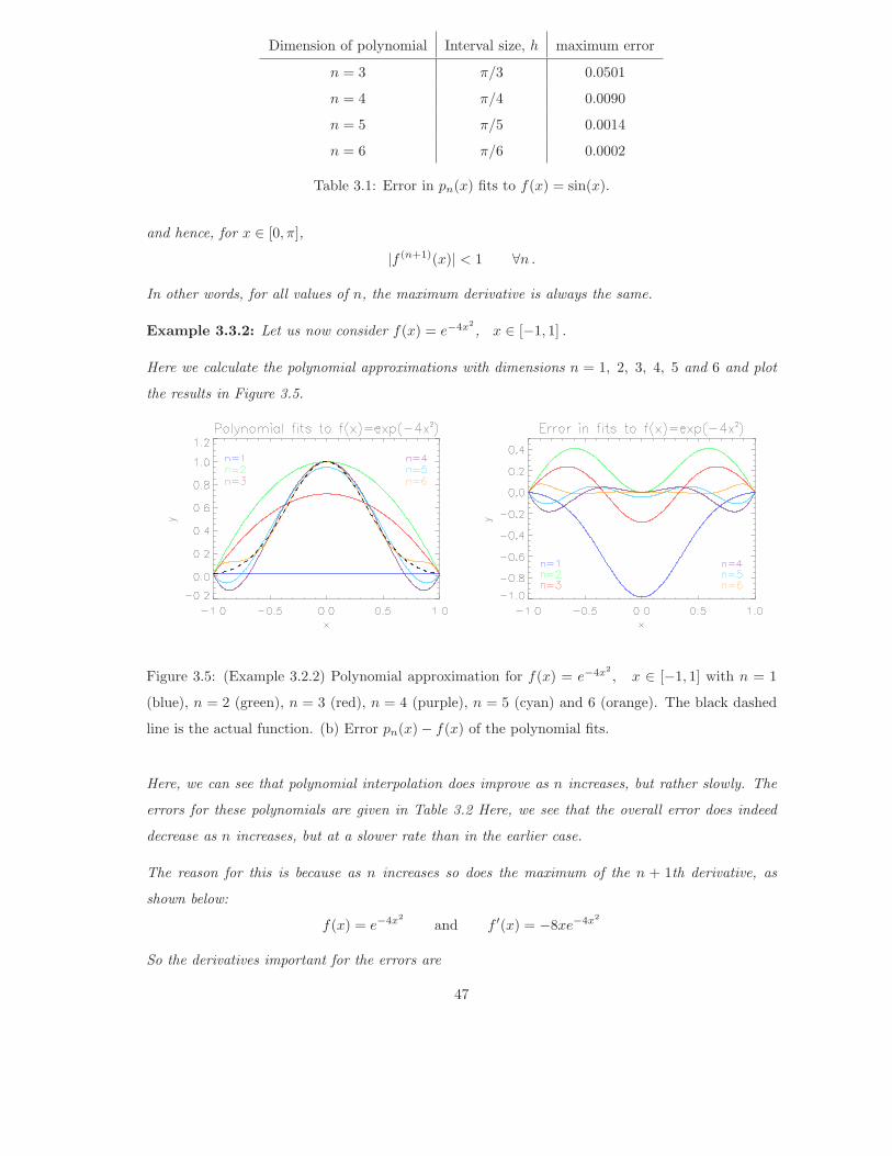
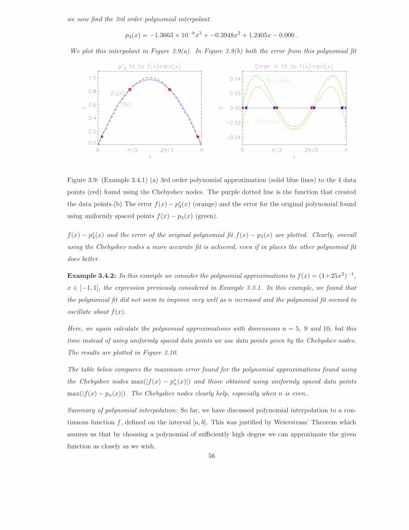
Example 3.5.3: In this example, we consider the cubic spline approximations to f(x) = (1 +

25x2)−1, x ∈ [−1, 1], the function previously considered in Examples 3.3.2 and 3.4.2. We will

compare our spline approximations found with the polynomial fits obtained for uniformly spaced data

points (Example 3.3.2) and data points obtained from the Chebyshev nodes (Example 3.4.2)

Here, we calculate the cubic spline approximations using (n+1) data points where, as before, n = 6, 9

and 10. The data points are uniformly spaced. The results are plotted in Figure 3.11.

67

Figure 3.16: (Example 3.5.1) (a) Cubic spline approximations for f(x) = 1/(1 + 25x2), x ∈ [−1, 1]

obtained using n+1 uniformly spaced data points with n = 6 (blue), n = 9 (green) and n = 10 (red).

The black dotted line is the actual function. (b) Error S3(x) − f(x) of the cubic Splines.

The table below compares the maximum error found for the polynomial approximations found using

the cubic splines max(|f(x)−S3(x)|), polynomials determined using the Chebyshev nodes max(|f(x)−p∗n(x)|) and polynomials obtained using uniformly spaced data points max(|f(x)−pn(x)|). The cubic

splines seem to give the best fits.

Dimension of polynomial max(|f(x) − S3(x)|) max(|f(x) − p∗n(x)|) max(|f(x) − pn(x)|)n = 6 0.1293 0.2642 0.6169

n = 9 0.1429 0.2691 0.3003

n = 10 0.0220 0.1091 1.916

68