An introduction to the quark model Jean-Marc Richard Université de Lyon & Institut de Physique Nucléaire de Lyon IN2P3-CNRS & UCB, 4 rue Enrico Fermi, 69622 Villeurbanne, France [email protected]May 25, 2012 Abstract This document contains a review on the quark model, prepared for lectures at the Niccolò Cabeo School at Ferrara in May 2012. It includes some historical aspects, the spectral properties of the 2-body and 3-body Schrödinger operators applied to mesons and baryons, the link between meson and baryon spectra, the role of flavour independence, and the speculations about stable or metastable multiquarks. The analogies between few-charge systems and few-quark bound states will be under- lined. Contents 1 Prelude: few charge systems in atomic physics 3 1.1 Introduction .................................... 3 1.2 The atomic two-body problem .......................... 3 1.3 Three-unit-charge ions .............................. 5 1.4 Three-body exotic ions .............................. 5 1.5 Molecules with four unit charges ........................ 6 2 A brief historical survey 7 2.1 Prehistory ..................................... 7 2.2 Early hadrons ................................... 7 2.3 Generalised isospin ................................ 9 2.4 The success of the eightfold way ........................ 10 2.5 The fundamental representation: quarks .................... 10 2.6 The OZI rule .................................... 12 2.7 First quark models ................................ 13 2.8 Heavy quarks ................................... 14 2.9 Confirmation ................................... 15 1 arXiv:1205.4326v2 [hep-ph] 24 May 2012
Transcript
An introduction to the quark model
Jean-Marc RichardUniversité de Lyon & Institut de Physique Nucléaire de Lyon
IN2P3-CNRS & UCB, 4 rue Enrico Fermi, 69622 Villeurbanne, France
AbstractThis document contains a review on the quark model, prepared for lectures at theNiccolò Cabeo School at Ferrara in May 2012. It includes some historical aspects,the spectral properties of the 2-body and 3-body Schrödinger operators applied tomesons and baryons, the link between meson and baryon spectra, the role of flavourindependence, and the speculations about stable or metastable multiquarks. Theanalogies between few-charge systems and few-quark bound states will be under-lined.
The spectrum of few-charge systems was among the very first applications of quantumphysics. The Bohr–Sommerfeld rules explain the energy levels of the hydrogen atom(p, e−), and can be easily extended to any (m+
1 ,m−2 ) pair with arbitrary masses. The so-
lution of the three-body problem for (m+1 ,m
−2 ,m
−3 ) turned out less obvious, and required
the Schrödinger equation, and the associated variational methods. It also revealed somesurprises, with the stability imposing constraints on the masses mi.
The stability of the positronium molecule (e+, e+, e−, e−), or any similar system withequal masses (in the limit where annihilation is neglected) was suggested by Wheelerin 1945 [1] and proved in 1947 [2], but the (indirect) experimental evidence was pub-lished only in 2007 [3]. This indicates how patient one should be when predicting novelstructures.
The quantum mechanics of few-charge systems was a great source of inspirationfor building the quark model, in its minimal non-relativistic version. Amazingly, sometechniques developed to extrapolate into flavour space the few-quark spectra with fla-vour-independent forces turned out useful to understand the stability patterns in atomicphysics. I refer to [4] for a review about few-charge systems. Here, I will just stress afew points that are connected to the quark model.
1.2 The atomic two-body problem
1.2.1 Central potential
Out of the Hamiltonianp2
1
2m1
+p2
1
2m1
− e2
r12
, (1)
the centre of mass can be removed and one is left with the intrinsic Hamiltonian de-scribing the relative motion, which reads
H =p2
2µ− e2
r, (2)
where µ is the reduced mass, given by µ−1 = m−11 + m−1
2 , and r = r2 − r1 and p =(p2 − p1)/2 are conjugate variables for the relative motion.
The Hamiltonian H has seemingly two parameters, the reduced mass µ and thestrength e2, but it can be rescaled. It is sufficient to solve once for ever the universalspectral problem
h = −∆− r−1 , (3)1if it is allowed to compare small things with great
4 AN INTRODUCTION TO THE QUARK MODEL
and to apply a simple factor 2µ e4 to the eigenvalues and (2µ e2)−1 to the distances torecover the actual energies and wave-functions of (2).
There is a similar universality for all harmonic oscillators p2/m + K r2, and moregenerally for all power-law interactions [5]
H =p2
2µ+ g ε(α) rα , (4)
where g > 0, ε is the sign function, to ensure that the force is attractive, and α is not toolarge if negative, otherwise the Hamiltonian would not be bounded from below.
A common feature of the Coulomb and Hookes potentials in three dimensions, isthat they support an infinite number of bound states, however weak is the strength ofthe potential. This contrasts with short-range potentials such as the Yukawa interaction−g exp(−b r)/r of nuclear physics, which requires a minimal strength g to achieve bind-ing. Similarly, the effective potential between neutral atoms or the effective potentialbetween two hadrons are of short-range nature, and thus do not necessarily supportbound states even when they are attractive.
The Coulomb Hamiltonian (3) has a well-known spectrum, with a discrete part εn,l =−1/[4 (n + `)2], where n = 1, 2, . . . is the radial number, and ` = 0, 1 . . . the orbitalmomentum (n+` is the principal quantum number). There is also a continuum for ε ≥ 0.
1.2.2 Spin-dependent corrections
The Coulomb interaction can be derived from Quantum ElectroDynamics (QED) in thenon-relativistic limit, and in the approximation of the lowest order in the coupling con-stant, which corresponds to one-photon exchange.
There are several interesting corrections, which have been probed successfully. Inparticular, the vector nature of the photon gives very characteristic spin corrections.
For ` ≥ 1, there are spin-orbit and tensor terms which contribute to the fine structure:levels with the same orbital momentum ` but different coupling of ` to the spins haveslightly different energies.
For ` = 0, there is spin–spin term, which splits the spin-singlet form the spin tripletstates. It reads
Vss =e2
m1m2
2π
3δ(3)(r)σ1.σ2 , (5)
in its most simplified form, to be treated at first order in perturbation theory, using thewave functions generated by the central potential−e2/r. The short-range character, andthe dependence on the masses should be kept in mind when an analogue will be pro-posed for the quark–antiquark interaction. This interaction is responsible for the shiftbetween the ortho- and para-hydrogen states and the transition between them producesthe famous 21 cm line, whose gravitational red-shift and Doppler shift gives valuable in-formation in astrophysics. The analogue will be measured at CERN for antihydrogen,to probe the matter–antimatter symmetry.
PRELUDE 5
Note that in the case of the positronium atom, the hyperfine splitting also receivessome contribution from the annihilation diagrams.
1.3 Three-unit-charge ions
The best known 3-body system is atomic physics is the neutral Helium atom, (α, e−, e−),but its stability is obvious since once the first electron is attached to the α particle, thereremains some long-range attraction to bind the second electron.
The binding of H− = (p, e−, e−) is less obvious, as the second electron feels a neutralsystem at large distances. Unlike the case of the Helium atom, neither an effective-charge ansatz ψ(r2, r3) = exp(−a(r2 + r3)), nor a more general Hartree wave functionf(r2) f(r3) suffices to demonstrate the binding variationally. But a more elaborate wavefunction does. For a review on two-electron systems, see, e.g., [6].
More interesting, perhaps, is the dependence upon the masses [4]: the molecularhydrogen ion H2
+ = (p, p, e−), is very stable, with a variety of excitations, the hydrogenion H− = (p, e−, e−) and the positronium ion Ps− = (e+, e−, e−) are bound by a smallmargin, but the “protonium ion” (p, p, e±) is not stable. (Here p and p simply denotesthe mass and the Coulomb charge; any hadronic interaction is neglected.)
There is an increase of stability near the symmetry line m2 = m3 of (m±1 ,m∓2 ,m
∓3 ).
Schematically, the system has there two threshold configurations (m+1 ,m
−2 ) + m−3 , and
(m+1 ,m
−3 ) + m−2 , which are degenerate, and thus interfere optimally to achieve the best
binding.This mass dependence is sometimes acute. For instance, a fictitious H− with one
electron heavier by about 10% would not be be stable. This is the case, e.g., for the(very) exotic (p, µ−, π−) ion.
1.4 Three-body exotic ions
It is sometimes believed that H− has no excited bound state. This is both true and false.This is true if you define a bound state as lying below the lowest threshold, which ismade of H = (p, e−) in the 1S state and an isolated electron. However, there is a levelwith total orbital momentum L = 1 and parity +1, that cannot break into H(1S) + e−
without involving spin forces and radiative effects. For this state, the lowest thresholdfor spontaneous dissociation consists of H = (p, e−) in the 2P state and an electron. Abound state lying below this threshold exists for H− = (p, e−, e−), but it exhibits evena more striking mass dependence when the constituents are modified [7]. Allowing avery small mass difference between the two electrons (less than 1%) or replacing theproton by a positron spoils the binding. On the other hand, if the masses are inverted,i.e., for the unnatural-parity state of H2
+ = (e−, p, p), a comfortable binding is observed.
6 AN INTRODUCTION TO THE QUARK MODEL
1.5 Molecules with four unit charges
The best known case corresponds to the hydrogen molecule H2 = (p, p, e−, e−), boundwell below the threshold for dissociation into two hydrogen atoms, with a variety ofexcitations. There are also variants with one or two protons replaced by an isotope. Themost suited framework for studying H2 is the Born–Oppenheimer approximation. Fora given position of the protons, the electronic energy is computed, and interpreted as aneffective proton–proton interaction supplementing their direct electrostatic repulsion.The Schrödinger equation is then solved for the two-body problem of the protons andgenerates the ground state and its radial and orbital excitations. Another set of levelscorrespond to the electron cloud being in an excited state. (Later the analogue will bethe hybrid hadrons, with the gluon field linking the quarks being excited). Note thatone hardly treats the hydrogen molecule as a “di-proton” bound to a “di-electron”.
In atomic physics and ab-initio chemistry, one usually starts from the limit where theproton and other nuclei are infinitely heavy, and then their finite mass can be treated as acorrection, through the Hughes–Eckart terms or similar. In 1945, Wheeler [1] addressedthe somewhat opposite issue of a proton with the same mass as the electron, i.e., theproblem of the stability of the positronium molecule, (e+, e+, e−, e−) (in the limit whereannihilation is neglected). In 1946, Ore performed an elaborate 4-body calculation, andconcluded that such a configuration is hardly stable [8]. But the following year, Hyller-aas and the very same Ore published an elegant analytic proof of the stability of thepositronium molecule [2]. It took 60 years to obtain at last an indirect experimentalevidence of the existence of this molecule [3].
Meanwhile the dependence upon the masses was studied in some details. In Refs. [9–12], it was shown how (M+,M+,m−,m−) gets more binding, as compared to its thresh-old, when the mass ratio departs from M/m = 1. On the other hand, it was observedthat when allowing for two different masses in another way, (M+,m+,M−,m−), stabil-ity is lost for M/m & 2.2 (or, M/m . 1/2.2), because the molecule cannot compete anymore with the lowest threshold (M+,M−) + (m+,m−) [13, 14].
Many less symmetric configurations are bound, such as the positronium hydridePsH = (p, e+, e−, e−), or any configurations in which two particles have the same chargeand the same mass, that is to say, (a+, b+, c−, c−), whatever are the masses of a and b [15].
The lessons, to be kept in mind when arriving at the section on multiquarks, are:
• the role of the masses is important. Look at (a+, b+, c−, d−) vs. its lowest thresholdsupposed to be (a+, c−) + (b+, d−). For both the 4-body system and its threshold,the potential energy
∑gij r
−1ij has a cumulated strength
∑gij = −2. So, there is
no obvious reason why a molecule should lie lower that two atoms. Hence anyfavourable breaking of symmetry in the kinetic energy is welcome. Conversely,any unfavourable breaking can spoil the binding.
• the four-body problem is delicate, even when the interaction is known perfectly,
• one should be patient to see the experimental confirmation of theoretical predic-tions of exotic states.
HISTORY 7
2 A brief historical survey
History is Philosophy teaching by examples2
Thucydid
2.1 Prehistory
There are several books relating the birth of particle physics, with entertaining anec-dotes. Segrè, for instance, was an acute observer [16]. A very comprehensive reviewis given by Pais [17]. For the nuclear forces, see [18]. Books and reviews devoted tothe quark model include [19–25]. There are also reviews covering baryons [26–28] ormesons [29–31], in particular the synthesis by the “quarkonium working group” [32,33].
After the Rutherford experiment, indicating how compact is the atomic nucleus, andthe discovery of the neutron by Chadwick, it became necessary to understand how thenucleus is built out of protons and neutrons. The mechanism of Yukawa: the exchangeof a massive boson, turned out the be successful, with the discovery of the pion at Bristolin 1947.
Among the theoretical activity stimulated by the Yukawa model, two points at leastdeserve attention.
1. The mass of the Yukawa boson is constrained by the ratio of the 3-body to the2-body binding energy, as stressed by Thomas in a celebrated paper [34], whoanticipated what is known today as “Borromean binding”, and, more generally,“Efimov physics”.
2. At first sight, three potentials are needed to build the nucleus: proton–proton,proton–neutron and neutron–neutron, and it is natural to seek for some simplifi-cation. A tempting scenario is that where solely the proton–neutron interactionexists, but this is clearly contradicted by the data on proton scattering. What even-tually prevailed is isospin symmetry. With the proton and the neutron forming adoublet, there are only two potentials in the limit where isospin is conserved, onefor total isospin I = 0, and another one for I = 1.
2.2 Early hadrons
The pion was discovered in 1947 and seen in three charge states, π+, π0, and π− whichform an isospin triplet. Hence in 1947, we had 5 hadrons: 2 nucleons and 3 pions.But already two more were expected, as the existence of antimatter was (not so easily)predicted as a consequence of the Dirac equation, and the positron was discovered incosmic rays by Anderson. The antiproton and the antineutron were anticipated as well.A dedicated accelerator was built at Berkeley, the Bevatron, and the antiproton was,indeed, discovered in 1955, and the antineutron shortly after.
2According to Michel Casevitz, the sentence is not by Thucydid, but a British commentator
8 AN INTRODUCTION TO THE QUARK MODEL
With 7 hadrons, 2 nucleons, 2 antinucleons, and 3 pions, the world of hadronicphysics would be reasonably sized, and one could envisage to work on the interactionamong these few hadrons. However, several complications occurred almost simultane-ously.
First, the Yukawa picture of nuclear forces, though very efficient for the long-rangepart, faced difficulties at shorter distances. More attraction was needed, and also somespin-orbit component, that neither pion-exchange or iterated pion-exchange were ableto provide. The work by Breit, among others, was remarkable [35]. For further details,see, e.g., the review [18]. An explicit scalar exchange (call it σ or ε) and an explicitvector exchange were needed. While the former was about isospin independent, andthus provided by the exchange of an isoscalar scalar meson, the latter was sought to bedifferent in np vs. pp scattering, and thus called for both an isoscalar and an isovectorvector meson. The ω and ρ were thus predicted!
Second, the interaction of pions with nucleons was shown to produce new parti-cles, nucleon resonances, in particular the ∆(1232), which has isospin 3/2, i.e., exists infour possible electric charges. Similarly, proton–nucleon or proton–nucleus scattering,or proton–antiproton annihilation were able to produce several new mesons, the onesdesired to improve the theory of nuclear forces, and others. These hadrons are not sta-ble, with for instance ∆→ N+π or ρ→ π+π, but were named hadrons as well, baryonsor mesons.
The ∆, at first sight, appears as a consequence of the interaction between π and N ,and the ρ as a resonance of the ππ interaction. Chew and his collaborators generalisedthis scenario, and suggested the concept of “bootstrap” or “nuclear democracy” [36,37]:everything is made of everything, and any hadron is both a building block and theresult of the interaction of the other hadrons. For instance, ∆ is made of Nπ, Nππ, etc.,and, as well N is made of ∆π, etc. This gives an infinite set of coupled equations, ofwhich it was hoped one could extract a finite set as a first tractable approximation to thespectrum and to the dynamics. The success was, however, extremely limited. Ball, Scottiand Wong, for instance, stressed that describing mesons as resulting of the nucleon–antinucleon interaction hardly gives the observed “exchange degeneracy” (named afterthe phenomenology of high-energy scattering), the property that an isoscalar and anisovector mesons with the same quantum numbers have very often the same mass [38].In the baryon sector, the next state after the ∆ with isospin I = 3/2 and spin J = 3/2was sometimes predicted to have I = 5/2 and J = 5/2!
Third came strangeness. New particles were observed in the 50s and 60s, decayingweakly though massive enough to decay to existing particles, and produced by pairswith strict rules: K+ together with Λ for instance, but never K− together Λ. A newquantum number, strangeness S, was introduced to summarise the properties of thesenew particles: strangeness is conserved in production processes by strong interaction,and thus Λ(S = −1) can be produced in association with K+(S = 1), but not K− whichhas S = −1. On the other hand, strangeness is not conserved in the decay by weakinteraction, as Λ(S = −1)→ N + π, or Λ→ p+ e− + ν. The weak interaction of strangeparticle was beautifully linked to that involved in ordinary beta decay.
HISTORY 9
2.3 Generalised isospin
There is of course the exception of the π meson, with a mass of about 0.14 GeV, signifi-cantly lighter than the mass of the K, about 0.49 GeV, and the exception of light scalarmesons with long-standing questions about their structure. Otherwise, one observesthat strange particles do not differ much form the non-strange ones. For instance, themass of the Λ baryon is about 1.1 GeV, just slightly above that of the nucleon at 0.94 GeV,and the mass of the K∗, 0.89 GeV, is close to that of the vector mesons ρ and ω, about0.78 GeV. It was thus tempting to put strange and non-strange particles in multipletsgeneralising isospin. Since isospin is built on the SU(2) group, the minimal extension isSU(3). Later, it was renamed SU(3)F, to differentiate it from the SU(3) group associatedwith colour.
A specific model was proposed by Sakata [39], with (n, p,Λ) as the building blocks ofmatter, and mesons as baryon–antibaryon pairs. We already mentioned that this pictureof mesons is difficult to accommodate with the long-range baryon–baryon interactionas given in the Yukawa picture. But the Sakata model had also problems with baryons.There are too many baryons with low mass. Take for instance the lowest baryons withspin J = 1/2. Besides p, n, and Λ, there is a triplet de singly-strange (S = −1) baryons(Σ+,Σ0,Σ−) of mass about 1.3 GeV, and a pair of doubly strange (S = −2) baryons(Ξ0,Ξ−) with mass about 1.5 GeV. In the Sakata model, they should belong to higherrepresentation, and, in a dynamical picture, contain an additional baryon–antibaryonpair. This is hard to believe.
To take care of this problem, Ne’emann and Gell-Mann suggested to keep the SU(3)group as the basic symmetry, but to put the known J = 1/2 baryons in an octet represen-tation. This is the famous “eightfold way” [40]. The group SU(3) has eight generators,instead of three for SU(2) (I± and I3). Each multiplet can be characterised by the dimen-sion of the representation (this generalises the 2 I + 1 multiplicity for SU(2)), and twogenerators that commute, which are usually taken as I3 and strangeness S, or equiv-alently the hypercharge defined as Y = b + S, where b is the baryon number. SU(3) is
I3
Y
•Σ− •Σ0 •
Σ+•Λ
•Ξ−
•Ξ0
•n •p
Figure 1: Octet of the lowest spin J = 1/2 baryons
rather good symmetry. Its breaking can be described by simple terms, treated at firstorder, which are proportional to some generators of the group. More elaborate mecha-
10 AN INTRODUCTION TO THE QUARK MODEL
nisms were proposed for breaking SU(3). One example is the famous Gell-Mann–Okuboformula for the baryon masses
M = M0 + a Y + b(I(I + 1)− Y 2/4) , (6)
from which one gets2(N + Ξ) = 3 Λ + Σ , (7)
where each particle stands for its mass, in surprisingly good agreement with experi-ment.
2.4 The success of the eightfold way
When the eightfold way was proposed, only 9 baryons with spin J = 3/2 were known,with a low mass: four ∆ of charge ranging from −1 to +2, thre Σ∗ with strangenessS = −1 and two Ξ∗ with strangeness S = −2. At the 1962 Rochester Conference heldin Geneva, Gell-Mann pointed out they would fit very well a decuplet representation ofSU(3), provided the last member does also exist. He named it Ω−, as a kind of ultimateachievement, in the biblical sense. The masses of the 9 existing members being observedto grow linearly with strangeness, i.e., following the pattern
Σ∗ −∆ = Ξ∗ − Σ∗ , (8)
known as the “equal spacing rule of the decuplet”, it was tempting to extrapolate to in-clude Ω−−Ξ∗ in the equality, thus predicting the mass of the Ω− at about 1.67 GeV. Somephysicists were sceptical about the possibility of producing and detecting easily the Ω−.It was nevertheless seen in an experiment at Brookhaven led by Nick Samios, with ex-actly the mass predicted by Gell-Mann. This was at the end of 1963, and published in1964 [41], which otherwise was one of the best vintages ever in Burgundy!
2.5 The fundamental representation: quarks
The pseudoscalar mesons (π, η, K, K) were accommodated in an octet and a singlet. Asthere is presumably mixing between the singlet and the isoscalar member of the octet,it became customary to talk about “nonet”. The same holds for the vector mesons. SeeFig. 3.
We thus had already in the hadronic world octets, singlets and decuplets, but notriplet, which corresponds to the fundamental representation! Gell-Mann proposed thatthe fundamental representation is populated by three yet not discovered – or hypothet-ical – particles. He was of course fully aware that any representation can be built bycombining the fundamental representation, 3, and its conjugate, 3, in the same way thatany value of the spin can be built by adding elementary spins 1/2.
The word “quark” was taken from the sentence “Three Quarks for Muster Mark” inJoyce’s Finnegans Wake. In another context (see next subsection), the word “ace” was
HISTORY 11
I3
Y
•Σ∗−
•Σ∗0 •
Σ∗+
•∆− •∆0 •∆++•∆+
•Ξ∗− •Ξ∗0
•Ω−
Figure 2: Decuplet of the lowest spin J = 3/2 baryons. The Ω− was missing till itsdiscovery in 1964.
suggested, but did not prevail. The individual quarks were sometimes named p, n andλ, in reference to the Sakata model, but quickly the naming scheme u, d, s was adoptedby the community.
The properties of the quarks are summarized in Table 1 and Fig. 4
Table 1: Properties of the quarks
q b I I3 Y S Q
u 13
12
12
13
0 23
d 13
12−1
213
0 −13
s 13
0 0 −23−1 2
3
I3
Y
•π−
•π0 •
π+•η•η′
•K−
•K0
•K0 •K+
I3
Y
•ρ−
•ρ0
•ρ+
•ω•φ
•K∗−
•K∗0
•K∗0 •K∗+
Figure 3: Octet and singlet of pseudoscalar (left) and vector (right) mesons.
12 AN INTRODUCTION TO THE QUARK MODEL
The basic reduction of products of representations that are important for the quarkmodel are
3× 3× 3 = 1 + 8 + 8 + 10 , 3× 3 = 1 + 8 . (9)
Historians could debate endlessly whether the pioneers considered quarks as a handymathematical tool to build the representation of SU(3), or had already in mind a phys-ical interpretation of the quarks as the constituents of the hadrons. Anyhow, this wasone of the major breakthroughs in physics.
I3
Y
•d • u
•s
I3
Y
• d•u
•s
Figure 4: Triplet of quarks and antitriplet of antiquarks
2.6 The OZI rule
Another approach was followed by Zweig. See, e.g., his recollection at the ConferenceBaryon80 [42] or at the celebration of Gell-Mann’s 80th birthday [43].
The φ meson, of mass about 1.02 GeV, was discovered in 1962 [44, 45]. It is anisoscalar, vector meson, like the ω, but with peculiar decay patterns. While it couldeasily decay into pions, it prefers the KK channels, for which the phase-space is mea-gre (the K has a mass of about 0.49 GeV).
Zweig’s explanation is that this favoured decay is dictated by φ meson content. Henamed the constituent “aces”, but we will call them quarks to conform with the currentusage. The idea is that the decay preferentially keeps the existing content. In the modernlanguage, the φ decay is described by the diagrams of Fig. 5.
φπ
ρ
φπ
ρ
φ
K
K
Figure 5: Decay of the φ meson: Zweig forbidden (left, centre) or allowed (right)
HISTORY 13
He thereby invented the “Zweig rule”, also called Okubo–Iizuka–Zweig (OZI), or(A–Z) rule since many authors contributed, from Alexander to Zweig. For a review, see,e.g., [46]. As we shall see shortly, a nice surprise was that the rule works even better forheavier quarks.
The rule governing the φ decay was extended to other decays and to reaction mecha-nisms. Quark lines should not start from and end in the same hadron, i.e., disconnecteddiagrams are suppressed. Instead quark lines should better link two hadrons in theinitial or final state.
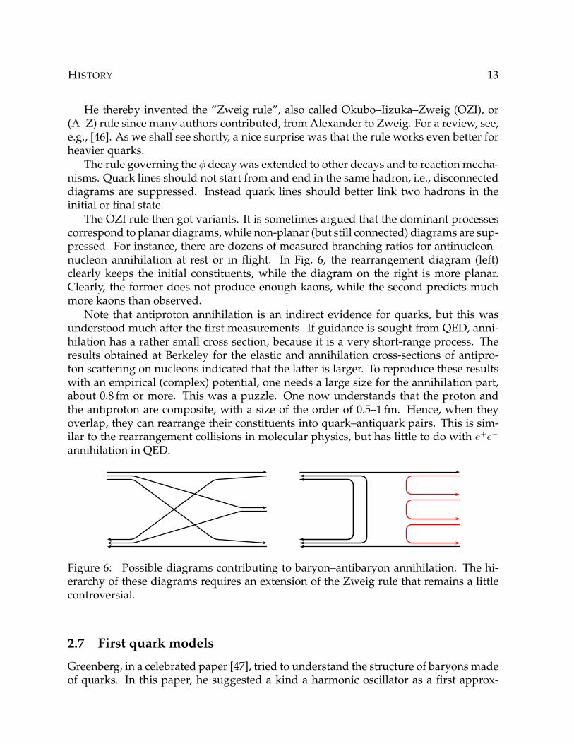
The OZI rule then got variants. It is sometimes argued that the dominant processescorrespond to planar diagrams, while non-planar (but still connected) diagrams are sup-pressed. For instance, there are dozens of measured branching ratios for antinucleon–nucleon annihilation at rest or in flight. In Fig. 6, the rearrangement diagram (left)clearly keeps the initial constituents, while the diagram on the right is more planar.Clearly, the former does not produce enough kaons, while the second predicts muchmore kaons than observed.
Note that antiproton annihilation is an indirect evidence for quarks, but this wasunderstood much after the first measurements. If guidance is sought from QED, anni-hilation has a rather small cross section, because it is a very short-range process. Theresults obtained at Berkeley for the elastic and annihilation cross-sections of antipro-ton scattering on nucleons indicated that the latter is larger. To reproduce these resultswith an empirical (complex) potential, one needs a large size for the annihilation part,about 0.8 fm or more. This was a puzzle. One now understands that the proton andthe antiproton are composite, with a size of the order of 0.5–1 fm. Hence, when theyoverlap, they can rearrange their constituents into quark–antiquark pairs. This is sim-ilar to the rearrangement collisions in molecular physics, but has little to do with e+e−
annihilation in QED.
Figure 6: Possible diagrams contributing to baryon–antibaryon annihilation. The hi-erarchy of these diagrams requires an extension of the Zweig rule that remains a littlecontroversial.
2.7 First quark models
Greenberg, in a celebrated paper [47], tried to understand the structure of baryons madeof quarks. In this paper, he suggested a kind a harmonic oscillator as a first approx-
14 AN INTRODUCTION TO THE QUARK MODEL
imation to describe the quark motion. He addressed the problem of the statistics andsuggested a kind of para-statistics, that eventually became the colour degree of freedom.
The work of Dalitz was done almost simultaneously. In the summer of 1965, and inparticular in his lectures at the School of Les Houches [48], he constructed his first ver-sion of the harmonic oscillator model of baryons. As Greenberg, he faced the problemof the statistics of the quark.
Dalitz’s work was the starting point of a series of studies about baryons in the har-monic oscillator model with contributions by Horgan, Hey, Kelly, Reinders, Gromes,Stamatescu, Stancu, Cutosky, etc., culminating with Isgur and Karl. Potential modelsnot based on harmonic confinement were proposed somewhat later. The references willbe given in the section on baryons.
Note also the contribution by Becchi and Morpurgo about the possibility of describ-ing hadrons made of quarks in a non-relativisitic approximation [19, 20, 49, 50].3
2.8 Heavy quarks
The physics of kaons has been very stimulating along the years: strangeness led tothe quarks, the θ − τ puzzle led to parity violation and to K0K0 mixing, whose de-tailed scrutiny revealed CP violation [17]. Another problem in the weak decay of kaonsinspired Glashow, Illiopoulos and Maiani [51], who predicted a fourth quark, named“charmed quark” and abbreviated as c, whose mass should not be too high. In someprocesses, diagrams involving a u and diagrams involving a c cancel out. This is theGIM mechanism.
A new spectroscopy was thus predicted, with charmed mesons such as (cu), orcharmed baryons such as (csu), double-charm baryons, etc. See, e.g., Gaillard, Lee andRosner [52]. Of course, (cc) mesons were predicted as well.
However, when in November 1974 (this was sometimes called the October revo-lution), the J/ψ was discovered simultaneously at SLAC and Brookhaven, and the ψ′
shortly after at SLAC, they were not immediately recognised as (cc), i.e., charmonium.The surprise was that they are extremely narrow resonances. We now understand thatthe Zweig rule works better and better when the quark become heavier. The spectrumof charmonium was completed with various P state, the ψ′′ = ψ(3770) which is a D state,and after some time, with the spin-singlet states.
Charmed mesons [53] and baryons [54] were discovered as well, and this sector isnow rather rich, tough the double- and triple-charm baryons still await discovery.
The charmonium gave a decisive impulse to the quark model in the meson sector.Thanks to Regge and others, we had already an idea about sequences of mesons withincreasing spin J . In the quark model, this corresponds to orbital excitations of thequark–antiquark motion. With charmonium, the new feature is that i) the levels arebetter seen, since the lowest states are narrow, ii) there is a clear evidence for the radial
3I thank Pr. Morpurgo for a correspondence related to this subject
HISTORY 15
degree of freedom. Explicit quark models were developed to describe the (cc) spectrum.They will be reviewed in Sec. 3.
At the time of the discovery of charm, in the 70s, there were already speculationsabout a symmetry between quarks and leptons. The light quarks (u, d) are the partnersof (e−, νe). The strange and charmed quarks belong in the family of (µ−, νµ).
Note that the leptons are ahead. The µ−was discovered in 1936,4 and was completelyunexpected (“who ordered the muon? asked Rabbi). The τ lepton was discovered atSLAC in 1977. The partners of the (τ−, ντ ) pairs were thus anticipated and named (t, b),as “top” and “bottom”. And a spectroscopy of hadrons containing b or t, or both, waspredicted. However, at a Conference in Hamburg, a German minister who had someknowledge of English, suggested to replace bottom by “beauty”. And t was renamed“truth quark”, but this is not very often used.
In 1977, Leon Lederman, who missed the charmonium by a small margin, did anexperiment similar to Ting’s, but with a more powerful beam and an improved detector,and announced in 1977 the discovery of the Υ and Υ′ particles, immediately interpretedas (bb) bound states [55, 56]. We shall come back in the next sections about the role offlavour independence. Just a word here. Lederman noticed that, within the precisionof his measurement, Υ′ − Υ ' ψ′ − J/ψ, and submitted to local theorists the questionwhether there exists a potential such that changing the reduced mass keep the spacings∆E unchanged (remember that ∆E ∝ m for the Coulomb potential and ∆E ∝ m−1/2
for the harmonic oscillator). Quigg and Rosner found that the logarithmic potential hasthis property for all spacings [57]. In fact, the logarithmic potential was already usedin empirical speculations about the not-yet-discovered bottomonium, but this propertywas not stressed clearly enough [58].
Predictions for (tt) were revised continuously, as the mass of the top was pushedhigher and higher by the negative results of the experimental searches. It was thenstressed (see, e.g., [59] for an early review) that if the top quark is very heavy, it willdecay before hadronising.
2.9 Confirmation
On the way from the early days of the quark model to the recent state of art, there aremany beautiful and decisive contributions that unfortunately, I cannot review here, dueto the lack of time. I will just list of few of them: deep inelastic scattering, the partonmodel, the MIT bag model, and its many variants, QCD, its property of asymptoticfreedom, lattice QCD, QCD sum rules, etc., etc.
4In 1947, the discovery of the pion was confused by the decay of pions into muons
16 AN INTRODUCTION TO THE QUARK MODEL
3 The quark–antiquark model of mesons
I married themFriar Laurence, Romeo and Juliet
3.1 Introduction
The quark model of mesons has not been developed “from the bottom up”, but mainly“from the charm down to light sector, and from the charm to the beauty quark”.
At the end of 1974, when the new particles seen at Brookhaven and SLAC wereidentified as (cc) bound states, explicit models were proposed to calculate the spectrumand the radiative transitions [60–63] . The potential proposed in [63] is know as thefunnel potential or Cornell potential, and reads,
V (r) = −ar
+ b r + c (10)
A new era of meson spectroscopy was opened, with explicit calculations of the mesonproperties in models which were first guessed empirically and are now more seriouslyinspired by QCD.
3.2 Quantum numbers
The total angular momentum J results from the coupling of the spin S of the quarksand their orbital momentum `, from which one also gets the parity (−1)`+1 and chargeconjugation C = (−1)`+S. The lowest states are given in Table 2.
Table 2: Quantum numbers of the lowest quarkonium states2 S+1`J
1S03S1
1P13P0
3P13P2
1D23D1
3D23D3
JPC 0−+ 1−− 1+− 0++ 1++ 2++ 2−+ 1−− 2−− 3−−
Comments are in order
• some sets of quantum numbers are absent. For instance, a state with JPC = 1−+
would be exotic,
• some JPC occur twice. There is the possibility of, e.g., 3S1 − 3D1 mixing, as for thedeuteron,
• the above quantum numbers are repeated for the radial excitations, labelled withthe radial number n. In the literature, one can find either n = 0, 1 . . . as in thefamiliar one-dimensional oscillator, or n = `+ 1, 2, . . . as in the Coulomb problem.In the latter case, the first P state is labelled 2P, the first D state 3D. We shall adoptn = 1, 2, . . ., i.e., a counting where the radial wave function has (n− 1) nodes.
MESONS 17
3.3 Spin averaged spectrum
With a potential such as (10) which is central, without spin dependence, the energydepends only on ` and n. The radial equation reads
− u′′(r) +`(`+ 1)
r2u(r) +mV (r)u(r) = mE u(r) , (11)
where m = mc is the mass of the charmed quark in the case of quarkonium, and other-wise m is twice the reduced mass. For a pure Coulomb interaction, this equation can berescaled to −v′′(r) + (`(` + 1)/r2 − 1/r − ε)v(r) = 0, with eigenenergies ε = −1/(4n2),with n = ` + 1, ` + 2, . . .. For a purely linear interaction, another rescaling leads to−v′′(r) + (`(` + 1)/r2 + r − ε)v(r) = 0, and in the case where ` = 0, it reduces to ashifted Airy equation: the eigenenergies are the negative of the zeros ai of the Airyfunction Ai(x), and the nth eigenfunction is just the very same Airy function shifted atan, vn(r) ∝ Ai(r + an), the normalised version being
vn(r) =Ai(r + an)
Ai′(an). (12)
If both the Coulomb and the linear terms are present, one can rescale to a one-parameterproblem, which can be chosen as[
−∆− λ
r+ r − ε
]ψ(r) = 0 , (13)
where λ can be expressed in terms of the quark mass m and the strength parameters aand b of the Cornell potential.
If the two-body problem is solved, one can tune the parameters to reproduce the lowlevels of charmonium. This was done by several groups in the late 70s, and the authorswere able to predict the missing states.
Note that this exercise did not provide with a sharp determination of the parameters,e.g., a, b and c in (10), and the mass mc of the charmed quark. Additional constraintswere used, such as the leptonic widths, and the rates of the γ-transitions. Still someflexibility was allowed, and, when the first bottomonium levels were found, the gamebecame more challenging: to reproduce simultaneously the (cc) and the (bb) spectra.
Indeed, even so the interquark potential was not derived from QCD in early quarko-nium phenomenology, it was assumed that it is universal, or “flavour independent”. InQCD the gluons couple to the colour. Hence it is reasonable to assume that the potentialis flavour independent.
We already mentioned the logarithmic solution for V (r) [57]. Then the radius scalesas m−1/2, and the square of the wave function at the origin, |φ(0)|2, that enter severaldecay widths, scale as m−3/2. As ln r = lim(rα − 1)/α as α→ 0, a generalisation consistsof a power-law interaction V (r) = Arα + B. Martin used this functional form to fit thequarkonium levels, and obtained a rather good fit [64] with a small value of α, i.e., apotential close to the logarithmic one. See, also, [65].
18 AN INTRODUCTION TO THE QUARK MODEL
A typical charmonium potential is shown in Fig. 7, as well as the reduced radialwave function u(r) for the 1S and 2S states. In units of GeV for V and GeV−1 for r, itreads V (r) = −.4/r+ 0.2 r− 0.35. It is just for illustration purpose, without any attemptto achieve the best fit.
1 2 3 4 5 6 7r
- 3
- 2
- 1
1
2
uHr L,V Hr L
Figure 7: Simple central potential −0.4/r + 0.2 r − 0.35 and two first S-wave levels for aquark mass mc = 1.5. Units are GeV for V , GeV−1 for r, and arbitrary for the reducedradial functions u(r).
The corresponding results are listed in Table 3. This should be considered as a kindof 0th order starting point which could be refined by tuning the parameters, fitting somehigher levels, and including some decay properties in the constraints.
Table 3: Rough fit to the spin-averaged levels of quarkonium (for 1D, the experimentalvalue corresponds to ψ′′ which is 3D1, and the state seen by CLEO [66] and BABAR [67],which is presumably 3D2
In Fig. 8 are shown the levels of bottomonium using the simple potential −0.4/r +0.2 r−0.35 and a massmb = 4.5 GeV. For the very beginners, its a good exercise to repro-duce these numbers. The hierarchy of the excitations corresponds to the observation.
In Fig. 9, we supplement the previous figure by the charmonium levels, computedwith the same simple potential. The 1S levels are arranged to coincide. The potential istuned to produce about the same spacing for the lowest states. But for the higher states,the spectrum becomes dominated by the linear part of the interaction, and the spacingis significantly higher for (cc) than for (bb).
MESONS 19
1S
2S
3S
1P
2P
1D
M (GeV)
-9.4
-9.8
-10.2
Figure 8: Predictions for the bb spectrum with a very simple potential.
M (GeV)
-
-
-
9.4
9.8
10.2
1S
2S
3S
1P
2P
1D
-
-
-
3.00
3.40
3.80
Figure 9: Comparison of the predictions for the bb (solid lines) and (cc) (dotted lines)levels with a very simple potential.
20 AN INTRODUCTION TO THE QUARK MODEL
3.4 Improvements to the potential
Perhaps, one should not try to improve too much the simple potential model of mesons.Take for instance proton–nucleus scattering in nuclear physics, where the so-calledGlauber approximation works very well. For years, many corrections have been es-timated, and each correction gave a large effect. At the end, one understood that themost important corrections cancel each other. There might be something similar in thequark model. Anyhow, let us list a few possible improvements.
3.4.1 More elaborate potentials
So far, we mentioned the simplest choices for the interquark potential, such as power-law, logarithm, or Coulomb-plus-linear.
The success of these empirical potentials, with a short-range part finite or less sin-gular than 1/r, and a confining part less sharp than r can be understood as follows: thesimplest interaction corresponds to a linear confinement, with a cigar-shaped gluon fluxlinking the two gluons, and a Coulomb-part to which one-gluon exchange contributes.But the linear part is smoothed by pair-creation effects; if one tries to increase the sep-aration between c and c, a pair of light quark is created, and this results in a softeningof the interaction [68, 69]. At short-distance, there is the asymptotic freedom, whichweakens the Coulomb term, see, for instance, the potential by Buchmuller et al. [70] orRichardson [71].
3.4.2 Relativistic corrections
The simplest potential models use the Schrödinger equation. However, the kinetic en-ergy turns out not to be very small as compared to the rest mass of the quarks. Modelshave been devised with a relativistic form of the kinetic energy
p2
2m→√m2 + p2 −m , (14)
See, e.g., Basdevant and Boukraa [72], Godfrey and Isgur [73], etc. This is of course justone step towards a fully relativistic and covariant picture, with retardation effects, etc.,one of the most serious attempts being the work of the Bonn group [74, 75], which lateralso described the baryons.
3.4.3 Strong decay of quarkonia
As already stressed, the miracle of charmonium and bottomonium is the suppressionof the decay into light hadrons, which proceeds through internal QQ annihilation intogluons and subsequent hadronisation of the emitted gluons. Hence the states below therelevant (Qq) + (Qq) threshold are narrow, and the states lying above easily decay intoa pair of flavoured mesons, by a Zweig-allowed mechanism.
MESONS 21
The most widely used model for describing (QQ) → (Qq) + (Qq) is based on quarkpair creation. For, say
A(q1, q2)→ B(q1, q3) + C(q3, q2) , (15)
a prescription is given for the creation of the extra pair (q3, q3), and the amplitude in-cludes the coefficients for the spin–isospin recoupling and the overlap of the wave-functions, say
M =
∫dτΨ(1, 2)O(3, 3) Ψ∗(1, 3) Ψ(3, 2) , (16)
where dτ is meant for all relative variables. The most popular is the co-called 3P0 modelproposed by Micu [76] and extensively used and developed by the Orsay group [77]and many others. The Cornell model of charmonium [78] is very similar.
The early applications were mostly for nodeless states, for which (16) gives someslight enhancement or suppression of |M|2 multiplying pure phase effects. The appli-cation to high charmonium states ψ(n) revealed more dramatic variations. In particular,if you consider the three OZI-allowed decays
ψ(n) → DD, D∗D + c.c., D∗D∗ , (17)
each, schematically, call for a certain momentum p in the initial-state wave function. Ifp lies at a node or a bump, the transition is suppressed or enhanced. On the basis ofsimple spin counting, one expects for (17) that the rates, divided by phase-space, areproportional to
R[DD, D∗D + c.c., D∗D∗] ∝ 1 : 4 : 7 , (18)
while the experimental results for ψ(4.04) show a clear dominance of D∗D∗. This led tosuggest a molecular structure for this ψ(4.04) [79] (see the section on multiquarks). Infact, the formalism of quark-pair creation shows that the decays into DD or D∗D + c.c.are suppressed by the node structure of the initial state [80]. See also, [81, 82]. In amore detailed analysis, Eichten et al. [83] and Fernandez et al. [84] concluded that thesituation is neither as simple a pure (cc) with nodes or a pure molecule, namely that thisstate is a charmonium with an abundant molecular component.5
3.4.4 Coupling to decay channel
The coupling to (Qq) + (Qq) also influence the energy and the internal structure of thequarkonia. The quark model is just a first approximation, with the minimal componentin Fock space, i.e., the first term in
|ψ〉 = a |cc〉+∑i
bi |ccqiqi〉+ · · · (19)
with the second term tentatively saturated by the lowest D(∗)D(∗) component and theDs analogues. In the model by Eichten et al. [78, 82], these contributions are generated
5I thank F. Fernandez for an interesting correspondence on this point
22 AN INTRODUCTION TO THE QUARK MODEL
from the main cc component by an explicit operator which creates a pair of light orstrange quarks out of the vacuum. This provides the states above the threshold with anexplicit decay width. The branching ratios are found to be in good agreement with theobserved ones. There is also a dispersive part, i.e., a shift of the energy due to mesonloops (see Fig. 10). If one introduces an explicit mass difference between D and D∗,these meson loops contribute to the fine and hyperfine splittings. See also [85], and therecent contributions by Barnes et al. [86], T. Burns [87], etc., where it is stressed that theloops with D, D∗, Ds, etc., tend to cancel one another.
(cc) (cc)
D(∗)
D(∗)
c
c
c
cq
q
Figure 10: Mesonic loop correction to the charmonium, seen at the hadron level (left) orquark level (right)
However, very close to the DD threshold, there is an effect on the ψ′, which cancouple to DD, while the η′c only couples to DD∗ + c.c. and D∗D∗. Hence the ψ′ − η′c issensitive to the coupling to virtual decay channels [88, 89].
We shall come back on these meson–meson configurations in the section on multi-quarks.
3.4.5 Fine structure
Three of the four members of the 1P level of (cc) were discovered rather early, thanks tothe transitions
ψ′ → χJ + γ , χJ → J/ψ + γ , (20)
with J = 0, 1, 2. The masses have later been measured with a very high precision usingan antiproton beam [90].
In the quark model, they are the spin triplet states 3P0, 3P1 and 3P2 (with a small ad-mixture of 3F2). The formalism for the splittings and for the electromagnetic transitionsis adapted from nuclear and atomic physics, and is reviewed, e.g., in Jackson’s lecturesat SLAC in 1976 [91].
The potential is written as
V (r) + Vss(r)σ1.σ2 + Vls(r) `.s+ Vt(r)S12 , (21)
where ` is the orbital momentum, s = (σ1 + σ2)/2 the total spin of the quarks, and thetensor operator is S12 = 3σ1.rσ1.r − σ1.σ2. If the two last terms in (21) are treated at
in terms of a an average triplet mass Mt and two matrix elements. This can be invertedas
Mt =1
9
[M(3P0) + 3M(3P1) + 5M(3P2)
],
〈Vls〉 =1
12
[−2M(3P0)− 3M(3P1) + 5M(3P1)
],
〈Vt〉 =5
72
[2M(3P0)− 3M(3P1) +M(3P1)
].
(23)
Note that if the spin-orbit and tensor terms are treated beyond perturbation theory,leading to the computed masses M(3PJ), and if Mt still denotes the computed resultwith only V (r) + Vss(r), then one gets
Mt ≥1
9
[M(3P0) + 3M(3P1) + 5M(3P2)
], (24)
i.e., Mt is above the naive weighted average. This should be kept in mind, when esti-mating the sign of Vss by comparing the spin-triplet states with the spin-singlet stategoverned by V (r)− 3Vss(r) (see below the paragraph on 1P1).
From the date of the Particle Data Group [92] on the 1P levels, of charmonium, (23)gives
and for 2PMt = 10.260 , 〈Vls〉 = 0.009 , and 〈Vt〉 = 0.002 GeV . (27)
3.4.6 Hyperfine splittings
This is a more delicate issue on the experimental side. The simple mechanisms explain-ing the fine structure (see next section) also predicted some hyperfine splitting, with apseudoscalar state named ηc about 0.1 GeV lighter than its vector partner J/ψ,. The ηcis the 1S0 state of (cc), with n = 1. It was thus anticipated that the M1 transition fromJ/ψ to ηc would not have a very large probability [93, 94].
A first candidate for ηc was claimed in Germany [95], with a surprising shift δ =m(J/ψ)−m(ηc) ∼ 0.3 GeV. Leutwyler and Stern [96] claimed that such a large shift was
24 AN INTRODUCTION TO THE QUARK MODEL
an unavoidable consequence of the relativistic character of the dynamics. In contrast,most potential builders predicted a smaller δ, once the first ηc was announced, recog-nized to face difficulties to accommodate such a large value of δ [97–101].
The German ηc was not confirmed [102], and instead, a more plausible one was seenat 2.980 GeV [103, 104], and confirmed in other places, including LEP and antiproton–proton collisions. The corresponding splitting is δ ' 0.116 GeV.
The ηc(2S), sometimes named η′c, was then predicted with a splitting δ′ = ψ′ − η′c ofabout 80 MeV. The ratio δ′/δ is mainly governed by the ratio R = |φ2(0)|2/|φ1(0)|2 of thewave function at the origin. This ratio can be estimated in potential models (for instance,this ratio is exactly R = 1 for a purely linear potential). It can also be deduced from theratio of the leptonic widths. The ηc(2S) was unfortunately forgotten in the elaborateCornell model with explicit account for the coupling to the virtual decay channels [82].This omission was repaired in [88,89], and the effect of meson loops found to be sizeable.The ηc(2S) does not couple to the nearbyDD, but the ψ′ does, and is pushed down. Thisreduces δ′. The ηc(2S) was eventually found at BELLE, BABAR and CLEO, in B decay,in γγ spectra and double-charmonium production [105–107]. It means that if one looksat e+e− → J/ψ + X and believes the Zweig rule, X is dominated by (cc), and, indeed,already known states have been seen in X as striking peaks. The ηc(2S) was confirmedin some other experiments. The splitting is ψ′ − η′c = 0.049 GeV.
From the very beginning, it was suspected that the hc, corresponding to the 1P1 stateof (cc), will be very difficult to produce. See, e.g., Renard [108]. In most models, hc ispredicted to lie very close to the centre of gravity of the spin-triplet, Mt. A first indi-cation was provided by the R704 experiment at CERN, the last experiment at the ISRring [109]. The hc was later found at CLEO (Cornell) [110] and E835 (Fermilab) [111].The mass of hc coincides with the centre of gravity of the triplet, and there is presumablya cancellation of several small terms.
The analogues in the (bb) family were also hard to find. We have now ηb, hb(1P ) andhb(2P ) in the particle listings [92]. Very recently, CLEO [112] reported a measurementof ηb(2S) and a confirmation of ηb(1S). The results are
1. The value of δ(1S) for (bb) was predicted by HPQCD [113] to be 70 ± 9 MeV. Ifyou cannot afford lattice QCD, you can attempt a poor-man estimate from (cc).Assuming a logarithmic potential, with the distances scaling as m−1/2, and a hy-perfine splitting proportional to |ψ(0)2|2/m2, one gets 6
δ(1S)bb = δ(1S)cc
(mb
mc
)−1/2
∼ 65 MeV . (29)
6I remember doing this computation using the cell phone of Kamal Seth in a fancy restaurant of Mu-nich
MESONS 25
2. The ratio of δ(1S) to δ(2S) drops from about 2.3 to about 1.4 in (cc) to (bb). Thisreflects how anomalously high is the ηc(2S) due to its vicinity of the OZI threshold.
3.4.7 The origin of the spin-dependent forces
The phenomenology of the spin-dependent forces in charmonium was greatly inspiredby QED and by nuclear forces.
It was early stressed that the one-gluon-exchange contribution to the cc interactionis very similar to the Coulomb interaction in QED, and thus is associated to the samespin corrections. The name “chromomagnetism” was given to the analogue of the mag-netic interaction. We shall come back on the important role of chromomagnetism in thesystematics of hyperfine splittings in ordinary hadrons [114] and in speculations aboutpossible multiquarks [115].
The one-meson-exchange picture of the nuclear forces, which was very popular inthe 60s and early 70s. The nucleon–nucleon potential was written V =
∑Vi, where each
Vi corresponds to a single partial wave in the t-channel, and thus gives a very specificspin dependence in the s-channel.
Schnitzer [97, 98], for instance, analysed the splittings assuming a vector meson ex-change, and a scalar confinement. Thus the 1/r terms gives spin-spin, tensor and spin-orbit terms similar to the terms describing the fine and hyperfine structure of atoms,or similar to the terms associated with ω exchange in nuclear forces. The term propor-tional to r gives a negative spin-orbit force. Several variants were discussed by variousauthors [100, 116, 117].
The method to reach full consistency of this approach was explained by Gromes(see, e.g., [118] for references) and Eichten and Feinberg [119]. The problem is that theeffective potential in the Schrödinger equation contains two types of contributions: anintrinsic spin dependence due to the nature of the exchanged object, and a relativis-tic effect known as Thomas precession. Even a scalar interaction, when reduced to aneffective non-relativistic potential, contains a central term and a related spin-orbit one.
3.4.8 Orbital mixing
The states with natural parity, except 3P0, contains two partial waves, which can mix.Let us consider JPC = 1−−. The wave–function reads
ψ =u(r)
r|3S1〉+
w(r)
r|3D1〉 , (30)
and after some algebra, it can be shown that the coupled radial equations read
−u′′(r)
m+ Vc(r)u(r) +
√8Vt(r)w(r) = E u(r) ,
−w′′(r)
m+
[6
mr2+ Vc(r)− 3Vls(r)− 2Vt(r)
]w(r) +
√8Vt(r)u(r) = E u(r)
(31)
26 AN INTRODUCTION TO THE QUARK MODEL
first derived many years ago for the deuteron. Here VC = V + Vss is the spin-tripletcentral potential. Solving (31) requires a regularisation of Vt(r) which behaves as r−3 atshort distances in most models. Often the result, for e.g., ψ′′ is written as [120]
ψ(3770) = a|3D1, n = 1〉+ b1|3S1, n = 1〉+ b2|3S1, n = 2〉+ · · · (32)
where the states in the r.h.s. are obtained by neglecting the coupling of the two equa-tions. One could debate whether b2 is larger than b1 because ψ′ lies very close to ψ′′, orb1 is larger due to the favourable node structure of J/ψ and ψ′′. This is not obvious: inatomic physics, the analogue of (32) requires a summation over all bi (in the discrete andcontinuous spectrum). See, e.g., [121, 122].
The orbital mixing is responsible for the coupling of ψ(3770) to e+e− that made itsobservation possible. It might also influence the pattern of its hadronic decays. See, e.g.,the discussion by Rosner [120].
Very likely, a good fraction of the orbital mixing is due to the coupling to decay chan-nels. For instance, the coefficients in (32) are estimated in [89], which uses an improvedversion of the Cornell model.
3.5 Summary for heavy quarkonia
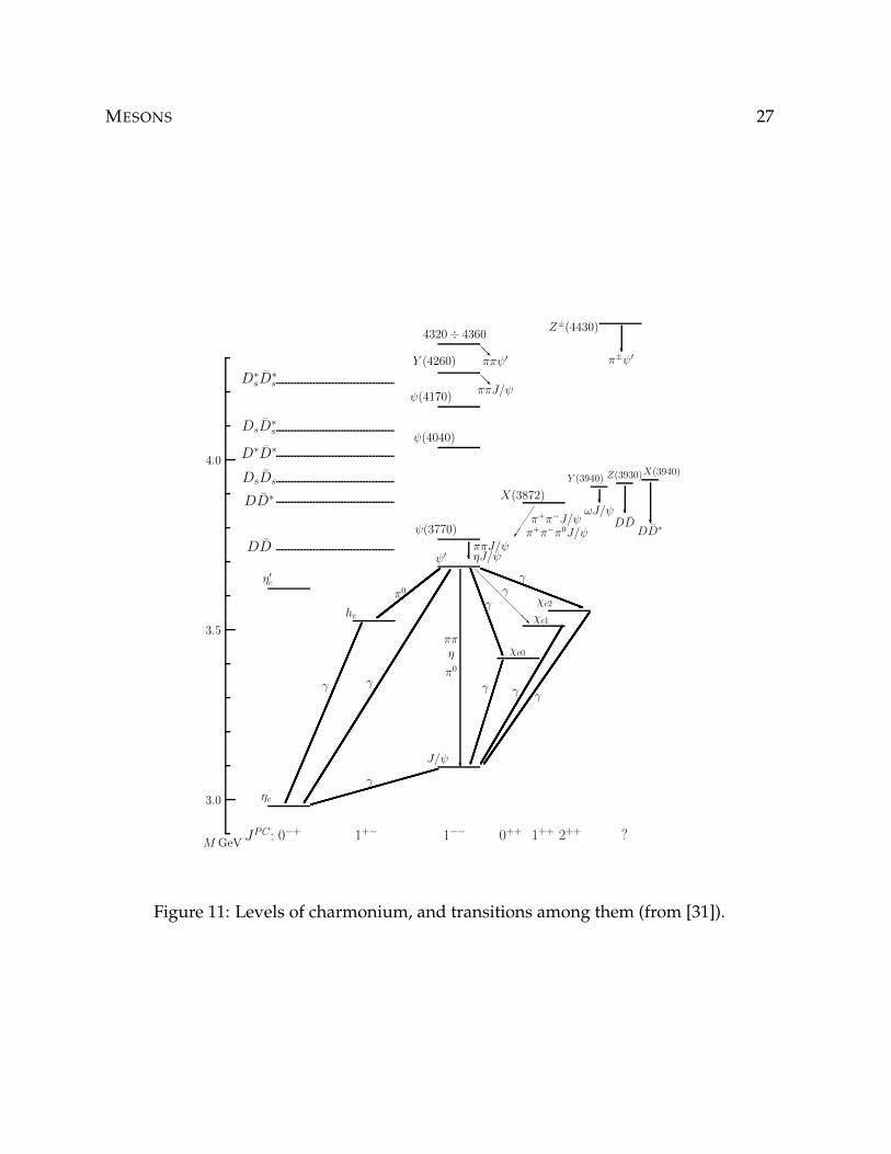
In Fig. 11, reproduced from [31] with the kind permission of the author, are shown thelevels of charmonium. The states labelled X , Y , Z will be discussed in another section.It is remarkable to see exactly the levels predicted by the quark model. On the left, thespin singlet states, with relative angular momentum ` = 0 for the two ηc, and ` = 1 forhc. In the middle, the various states with spin triplet, and ` = 0, 1, and even one examplewith ` = 2, and the various recoupling of spin and orbital momentum. The hierarchyof orbital vs. radial excitations, and the patterns of fine and hyperfine splittings arenow well described with simple potentials that are now better understood from theunderlying QCD.
MESONS 27
Y (3940) Z(3930)X(3940)
ωJ/ψDD
DD∗
??
?
@@RππJ/ψ
@@Rππψ′
?π±ψ′
Z±(4430)4320÷ 4360
?
q
@@@
@@@@R
N
9
=
JPC : 0−+ 1+− 1−− 0++ 1++ 2++ ?
ηc
η′c
hc
J/ψ
ψ′
χc0
χc1
χc2
ψ(3770)
X(3872)
ψ(4040)
ψ(4170)
Y (4260)
γγ
γ
γγγγ
γ
ππη
π0
π0
γ
π+π−J/ψπ+π−π0J/ψ
DD
DD∗DsDs
D∗D∗
DsD∗s
D∗sD
∗s
3.0
3.5
4.0
M GeV
?ππJ/ψηJ/ψ
Figure 11: Levels of charmonium, and transitions among them (from [31]).
28 AN INTRODUCTION TO THE QUARK MODEL
(2S
)ψ
γ∗
η c(2S
)
η c(1S
)
had
rons
had
rons
had
ronsh
adrons
radiative
had
rons
had
rons
χ c2(1
P)
χ c0(1
P)
(1S
)ψ
J/
=J
PC
0−+
1−−
0++
1++
1+−
2++
χ c1(1
P) π0
γ γγ
γγ
γ
γγ∗
hc(1
P)
ππη,
π0had
rons
=
BB
th
resh
old
(4S
)
(3S
)
(2S
)
(1S
)
(108
60)
(110
20)
had
ron
s
had
ron
s
had
ron
s
γ γ γ γ
η b(3S
)
η b(2S
)
χ b1(1
P)
χ b2(1
P)
χ b2(2
P)
hb(2P
)
η b(1S
)
JPC
0−+
1−−
1+−
0++
1++
2++
χ b0(2
P)
χ b1(2
P)
χ b0(1
P)
hb
(1P
)
Figu
re12
:Cha
rmon
ium
and
bott
omon
ium
spec
tra.
Borr
owed
from
PDG
[92]
.So
me
stat
esin
dica
ted
bya
dott
edlin
eha
vebe
enid
enti
fied
rece
ntly
.
MESONS 29
In Fig. 12, we reproduce the lower part of the charmonium spectrum, and the bot-tomonium spectrum, borrowed from the Review of Particle Properties [92].
The spectra are very similar. This is due to the property of flavour independence.The differences are also understood, due to explicit mass-dependence of the fine andhyperfine terms.
3.6 Light mesons
The simple quark model is in principle not applicable to light quarks, but some reck-less attempts were encouraging. For instance, Martin [64] managed to fit (bb), (cc), (ss)and (cs) with a single potential. The game was extended further by Bhaduri et al. [123],however their uniform regularisation of the hyperfine interaction gave poor predictionsfor J/ψ − ηc and similar splittings. Their model was refined by several authors, see,e.g., [124], with a regularisation of spin forces that depends on the system under con-sideration.
Isgur et al. [125] have explained why there are some good reasons to link potentialmodels, with a minimal amount of relativity, to the underlying QCD.
Let us give two examples. The first positive-parity excitations of (qq) with I = 1are a0(980), b1(1235), a1(1260) and a2(1320). In the quark model, they correspond to thepartial wave 3P0, 1P1, 3P1 and 3P2. The level order of this 1P multiplet, and even thepattern of spacings is very similar to what is observed in the charmonium 1P states.
If one looks at meson with high spin J and plot the square mass M2 against J , onefinds an almost perfect linear behaviour for this “Regge trajectory”. If a linear poten-tial is plugged into a Schrödinger equatiion with relativistic kinematics, this linear be-haviour is reproduced.
3.7 Heavy-light mesons
This is an even more dangerous playing ground. Remember, for instance, that an elec-tron is more relativistic in the hydrogen atom, (p, e−), than in the positronium atom,(e+, e−). There is nevertheless a very interesting spectroscopy of D and B mesons.
In first approximation, the reduced mass governing the internal dynamics is thesame for (cq) and (bq) mesons, so the excitation spectra should be very similar. This israther obvious in potential models, but it remains valid much beyond this framework.This is one of aspects of “heavy quark symmetry” [126–128].
3.8 Mathematical developments
The quark model motivated some studies about the properties of the Schrödinger oper-ator with confining interactions. See, e.g., [25, 129] for a review and references.
Among the subjects, let us mention the following.
30 AN INTRODUCTION TO THE QUARK MODEL
3.8.1 Level order
A sufficient condition has been derived that transforms the Coulomb degeneracy
E(1, `) = E(2, `− 1) = · · · = E(`+ 1, 0) , (33)
into a series of inequalities: the condition is related to the sign of the Laplacian of thepotential. As ∆V > 0 for the funnel potential (13) or any plausible interquark potential,this theorem explains the observed 1P < 2S ordering in quarkonium, and 2P < 3S inbottomonium. Note that ∆V ≤ 0 for the last electron of an alkalin atom and ∆V ≥0 for a muon inside a nucleus: this explains the observed breaking of the Coulombdegeneracy for alkalin atoms and muonic atoms.
Similarly, the sign of the second derivative of the potential as a function of r2 governsthe breaking of the HO degeneracy,
E(1, `) = E(2, `− 2) = E(2, `− 4) = · · · . (34)
This explains why 2S < 1D, i.e., m(ψ′) < m(ψ′′).There are also results on the spacing of levels as a function of the radial number.
For the harmonic oscillator, there is a remarkable equal spacing, E(n+ 1, `)− E(n, `) =E(n, `)− E(n− 1, `). For a linear potential, the spacing decreases.
3.8.2 The wave function at the origin
Many decay widths are proportional to the square wave function at the origin, whichfor S-states, reads
pn = |Φn(0)|2 =1
4 πu′n(0)2 . (35)
if the reduced radial wave function is arranged to be real. The studies on quarkoniumgave the opportunity to remember the rule by Schwinger (see, e;g., [129])
u′(0)2 = 2µ
∫ ∞0
dV
dru2(r) dr . (36)
This explains why the pn are independent of n for a purely linear interaction, and, con-versely, why the normalisation factor in (12) is given by the derivative.
There are sufficient conditions ensuring that pn increases or decreases as a functionof n [25].
3.8.3 The dependence upon the masses
If flavour independence is accepted as a strict rule, one has to study how the energylevels and the wave functions evolve when the reduced mass is modified.
As the kinetic energy term is p2/(2µ), obviously E as µ . The effect is pro-nounced when going from (cc) to (bb). On the other hand, the reduced mass governing
MESONS 31
(Qq) does not change much from Q = c to Q = b. Hence the OZI threshold (Qq) + (Qq)has almost the same energy for Q = b and Q = c. This explains why the Υ(1S) is moredeeply bound than J/ψ with respect to this threshold, and why there are more narrowstates in the bottomonium spectrum than in the charmonium one.
One can go further and notice that in a strictly flavour-independent interaction, theinverse reduced mass enters linearly. There is a known result that for an Hamiltoniandepending linearly on a parameter, say H = A + λB, the ground state energy ε0, orthe sum of first energies
∑Ni=0 εi is a concave (or convex upward) function of λ. Once
the constituent masses are added, this implies for the ground state of each angular-momentum sector,
(QQ) + (qq) ≤ 2(Qq) , (37)
an inequality independently derived by Martin and Bertlmann [25, 130] and Nussinov[131, 132] for potential models, and extended much beyond this framework [132, 133].Early applications introduced dangerously light quarks, but still, the inequality is satis-fied for the spin-triplet states of (cc), (ss) and (cs). Safer is the prediction that the (spinaveraged) ground state of (bc) is above the middle of (cc) and (bb).
Note that in atomic physics, it is reasonable to believe that the Born–Oppenheimerpotential that binds di-atomic molecules remains unchanged if the nuclei are replacedby isotopes. Thus (37) holds for H2, D2 and HD, and this governs their abundance atthermodynamic equilibrium [134].
3.8.4 Concavity with respect to the spin coefficients
In the same vein, one can explain the sign of the error when treating the spin correctionsto first order. For the hyperfine effect of S-state alone the singlet and triplet Hamiltoni-ans are respectively, in an obvious notation,
Hs = H0 − 3Vss , Ht = H0 + Vss , (38)
so that the fictitious eigenstate of H0 alone lies at
E0 ≥1
4Es +
3
4Et . (39)
Note that the inclusion of the tensor force would slightly lower Et, with 3S1 becoming3S1 − 3D1.
It is straightforward to extend this to the case of two parameters. Consider thegeneric spin-triplet Hamiltonian
HJ = Ht + αJ Vls + βJ Vt , (40)
so that H0 + 3H1 + 5H2 = 9Ht, then the fictitious spin-triplet state free of spin-orbit andtensor corrections lies at
Et ≥ [EJ=0 + 3EJ=1 + 5EJ=2] /9 , (41)
32 AN INTRODUCTION TO THE QUARK MODEL
i.e., above the naive centre of gravity, as discussed earlier in this section. Thus if the 1P1
is found at the location of the naive of gravity, it has received some attractive spin–spindownward shift.7
4 BaryonsTres faciunt collegium8
Latin sentence4.1 Introduction
The quark model of baryons was developed in the 60s, in particular by Dalitz and hiscollaborators, and several other groups, at a time when many nucleon and hyperonresonances were already known.
These early studies, and the more recent work by Isgur and Karl, Gromes et al.,Stancu et al., Cutosky et al., cannot be separated from the harmonic oscillator (HO)model, which provides a powerful classification scheme, and an efficient tool to imple-ment the symmetry constraints. This is reviewed, e.g., by Hey and Kelly [135].
The HO model has reached a high degree of refinement, with all the possible correc-tions carefully listed, and their tentative interpretation in QCD (one-gluon-exchange).
There has also been attempts to solve the three-body problem, using known tech-niques developed in atomic or nuclear physics, such as Faddeev equations, hyperspher-ical harmonics or variational methods. Then any potential can be used, for instance afunnel interaction with a superposition of Coulomb and linear contributions.
Note that in most early studies, it was implicitly assumed that the potential is pair-wise, and the question has been addressed of the link between the interquark poten-tial in baryons and the quark–antiquark potential in mesons. This will be discussed inSec. 4.12. In fact, it has been anticipated for many years, that the confining interactionis of three-body nature, i.e., depends simultaneously upon all relative distances. Thismakes the calculations technically more involved, but makes a link with the lattice QCDwhich favours such potentials [136].
The role of relativistic effects is of course important. In the latest works by Isguret al., a relativistic kinematics was adopted [137]. There are even models based on theBethe–Salpeter equation [138].
4.2 Jacobi coordinates
In the case of equal masses, a set of Jacobi coordinates that diagonalise the kinetic energyis (see Fig. 13)
R =r1 + r2 + r3
3, x = r2 − r1 , y =
2 r3 − r1 − r2√3
, (42)
7I remember discussions on this point at a Workshop organised in Genoa, to celebrate years of charmphysics with antiprotons, and later with Kamal Seth.
8Three makes a company
BARYONS 33
b
q1
b
q2
b q3
b
x√3y/2
Figure 13: Jacobi coordinates for the relative motion of the quarks inside a baryon
where the factor in y makes it easier to implement the symmetry constraints, as ex-plained shortly. Then, once the centre of mass motion is removed, the intrinsic Hamil-tonian reads
h =p2x
m+p2y
m+ V (x,y) , (43)
where the potential energy, already written as translation-invariant, has to be scalar.In the case of two different masses, say (m,m,M), R is modified, but one can keep
x and y as above. Then the intrinsic Hamiltonian becomes
h =p2x
µx+p2y
µy+ V (x,y) , (44)
with the reduced masses now given by
µx = m , µ−1y = (m−1 + 2M−1)/3 . (45)
If the three masses are unequal, the Jacobi coordinate y becomes y ∝ (m1 + m2)r3 −m1 r1 −m2 r2, and it is straightforward to derive the reduced masses µx and µy as func-tions of the individual masses mi.
Later in this section, we shall elaborate more on the potential energy V . Let us justmention here two popular choices. The harmonic oscillator corresponds to V = K(r2
12 +r2
23 +r231), where rij = |rij| and rij = rj−ri. It becomes V = 3K(x2 +y2)/2 for (m,m,m)
and (m,m,M), and a more complicated quadratic form of x and y for (m1,m2,m3). Thepairwise models reads v(r12) + v(r23) + v(r31).
4.3 Permutation symmetry
Schematically, the wave function of a baryon in the quark model is
Ψ = ψ(x,y)ψs ψi ψc , (46)
with orbital, spin, isospin and colour parts, and this wave function has to be antisym-metric with respect to the permutation of the identical quarks.
34 AN INTRODUCTION TO THE QUARK MODEL
If there are two identical quarks, as in Ξ− = (ssd) or in Λ = (uds) in the limit whereisospin symmetry is exact, then each term in (46) is either symmetric or antisymmetric.For the ground state of Λ, with isospin I = 0, the colour, spin and isospin parts areantisymmetric and the orbital part symmetric. This means spin 0 for the light quarks,and thus s = 1/2 for the three quarks, isospin I = 0, and ψ(x,y) even in x. For instance,in the harmonic oscillator, ψ(x,y) ∝ exp[−ax2 − by2].
There are two type of P-states: one where the degree of freedom associated to λ isexcited, with the same symmetry pattern as the ground state. Another wave where thelight quarks have their spin coupled to sqq = 1, and the orbital wave function ψ(x,y) isodd in x. In the harmonic oscillator, the orbital wave functions are of the type
y exp[−ax2 − by2] , x exp[−ax2 − by2] . (47)
For the former, the quark spin s = 1/2 and the angular momentum `y gives a baryonspin J = 1/2 or J = 3/2. For the latter, both s = 1/2 and s = 3/2 are possible, and thusa variety of values for the spin J . Usually, the spin orbit splittings are small in baryons(see below), and the states with various combinations of spins and angular momenta arenearly degenerate. One exception is the Λ(1405) − Λ(1520) pair, which has motivatedan abundant literature. The most plausible explanation is the coupling of one of thesestates to a nearby threshold.
For three identical quarks, imposing the constraints of antisymmetrisation is moredelicate. The colour coupling 3 × 3 × 3 → 1 is antisymmetric, thus the rest of the wavefunction should be symmetric. This was, indeed, one of the motivations for introducingcolour. For the Ω−, this is rather simple: the spin wave-function is symmetric, isospindoes not exists, and the orbital wave function is symmetric. For instance, ψ(x,y) =exp[−a(x2 + y2)] in the HO case. This is similar for the ∆(1232) multiplet, as the isospincoupling 1/2× 1/2× 1/2→ 3/2 is symmetric.
For the first parity excitations of Ω−, with JP = (1/2)− or (3/2)−, the spin and theorbital wave functions are neither symmetric nor antisymmetric, but their combinationis symmetric. One cannot escape here to introduce the concept of mixed symmetry. Theprototype is given by the Jacobi coordinates x and y of (42). The permutation P12 revealsx odd and y even, but a circular permutation P→ gives
P→[y + ix] = j [y + ix] , (48)
where j = exp(2 i π/3), as usual. Obviously, if two pairs, say z = v + i u and Z =V + i U , have the same permutation properties as z = y + ix, then their coupling givea symmetric term, and antisymmetric one, and a new pair of mixed symmetry (again inthe complex notation), respectively
<e[z Z∗] = uU + v V ,
=m[z Z∗] = v U − uV ,
[z Z]∗ = (uU − v V )− i (uV + v U) .
(49)
BARYONS 35
In the case of the P-states of Ω−, we have a pair of mixed-symmetry orbital wavefunctions, ψx, ψy, with either x or y excited, which for the harmonic oscillator readψx, ψy = x,y exp[−a(x2 + y2)], and a pair of spin 1/2 wave functions
Sx =1√2
[↑↓↑ − ↓↑↑] , Sy =1√6
[2 ↑↑↓ − ↑↓↑ − ↓↑↑] , (50)
which bears an obvious analogy with the Jacobi variables (42). With a spin-independentinteraction, the P-states of Ω− have a wave function of the type [ψx Sx + ψy Sy]/
√2.
For the nucleon ground state, the orbital part is symmetric, but the spin and isospinparts are both of mixed symmetry, with (50) for the spin, its analogues Ix, Iy forisospin, and the combination [Sx Ix + Sy Iy]/
√2 being symmetric.
The most interesting example of baryon in this respect consists of the antisymmet-ric spin–isospin wave function [Sx Iy − Sy Ix]/
√2 which requires a fully antisymmetric
orbital wave function. This wave function is excited in any interquark separation. Forinstance, in the specific case of the harmonic oscillator, it reads x× y exp[−a(x2 + y2)],i.e., `P = 1+. This is one of the states predicted in the three-quark model and absent inthe quark-diquark model. See below the section on diquarks.
4.4 Solving the three-body problem for baryons
4.4.1 The harmonic oscillator
After rescaling, the linear oscillator reads h = p2 + x2 with energies εn = 1 + 2n andwave functions ϕ0(x) ∝ exp(−x2/2) and ϕn(x) ∝ [−d/dx+ x]n ϕ0(x).
For equal masses m, the three-body problem with V = 2K/3(r212 + r2
23 + r231) is gov-
erned by the Hamiltonian
H(m,m,m) =p2x
m+p2y
m+K(x2 + y2) , (51)
which corresponds to a sum of two independent spatial oscillator, or six linear oscilla-tors. The energies E = (6 + 4nx + 2`x + 4ny + 2 `y)
√K/m have a cumulated number
of excitations N = 2nx + `x + 2ny + `y. Here, the radial and orbital excitations in eachvariable are counted separately.
There is a considerable degeneracy of the levels of given N ≥ 2, which contains con-tains several JP states. The literature on baryons within HO has developed a system-atic notation which is used beyond this model. In particular, the multiplets are denoted[d, `P ](n), where d is the spin–flavour multiplicity, ` the total orbital momentum, and (n)the radial occurrence (n = 0 is omitted). For instance, the ground state is labelled as[56, 0+], and the Roper resonance and its partners [56, 0]′. The ground state contains theoctet of Fig. 1 and the decuplet of Fig. 2, i.e., 2× 8 + 4× 10 = 56 states. The first orbitalexcitation is [70, 1−], and the first state with a full antisymmetric orbital wave functionis [20, 1+].
36 AN INTRODUCTION TO THE QUARK MODEL
The case of two different masses reads
H(m,m,M) =p2x
m+p2y
µ+K(x2 + y2) , (52)
with µ given by (45). There is still an exact decoupling, and the energies are
E(m,m,M) =
√K
m(3 + 4nx + 2 `x) +
√K
µ(3 + 4ny + 2 `y) . (53)
Here the lowest excitation is explicitly associated with the heavier quark(s),i.e., this isan excitation in the vecx variable. This point will be further discussed in the section ondouble-charm baryons.
The case of three different masses is also solvable exactly, though this is slightly lessknown.9 Once the kinetic energy is written as (44), one can use a rescaling x → x/
õx
and y → y/√µy. The Hamiltonian becomes
H(m1,m2,m3) = p2x + p2
y + Ax2 +B y2 + 2C xy , (54)
and one is left with the diagonalisation of a 2× 2 matrix.
4.4.2 First-order perturbation around the harmonic oscillator
We now turn to more general models for the interaction. The most spread methodconsists of writing the potential as
V = K(x2 + y2) + δV , (55)
and treat the second term as a perturbation. If K is optimised, this is the first stepof a variational expansion, to be discussed below. This is of course not very accurate,especially at short distances. If δV tentatively pushes down the Roper resonance (to bediscussed shortly) from the N = 2 level of the harmonic oscillator to the vicinity of theN = 1 level, then perturbation theory is in principle not applicable, as it requires thatthe shifts are small compared to the initial spacings.
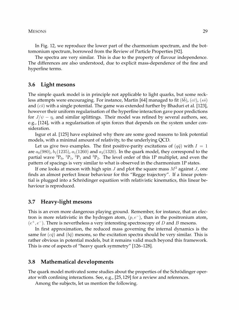
Isgur and Karl [139] have noticed the nice patterns of the N = 2 multiplet splittingwhen perturbed by a pairwise δV . It is illustrated in Fig. 14. Gromes and Stamatescu[140] pointed out that the upper part survives if the HO is perturbed by a symmetric3-body potential, while the [56, 0+]′ decouples. The same conclusion was reached byTaxil et al. [141], in the more general situation of a nearly hypercentral potential.
The upper part of Fig. 14 fits rather well the spin-averaged values of the observa-tions.
This pattern and the one for the N = 3 multiplet have been further discussed byTaxil et al. [141], Stancu et al. [142], etc.
9I remember discussions on this point with J.-L. Basdevant, and with D.O. Riska
BARYONS 37
0.5∆
0.1∆
0.2∆
0.2∆
[56, 0+]′
[70, 0+][56, 2+]
[70, 1+]
[20, 1+]
Figure 14: Splitting pattern of the N = 2 multiplet for a two-body perturbation ofthe harmonic oscillator. [Check whether the 2-body character is required.] There isan overall shift (not shown), and, in addition, a shift 0.1∆, 0.2∆, 0.3∆ or ±0.5∆ of thesublevels.
4.4.3 Converged variational methods
Let us consider the ground state with equal masses, but the generalisation to unequalmasses is straightforward. The above method can be read as the first term in a system-atic expansion
Ψ(x,y) =∑n
cn φn(x,y) , (56)
where n denotes the number of excitations and other quantum numbers associated tothe solutions φn(x,y) of the harmonic oscillator. The matrix elements can be calculatedwith subtle recursion relations. The convergence as a function of the maximal n is ex-cellent for the energy but elusive for the short-range correlations.
A variant is the so-called Gaussian expansion, widely used in theoretical chemistryand other quantum problems. It reads
Ψ(x,y) =∑i
γi exp[−(ai x2 + biy
2 + 2 ci x.y)] . (57)
Note that the permutation symmetry is violated in an individual term if ai 6= bi andci 6= 0, but is restored in the summation either explicitly (correlated Gaussians) or by thenumerical adjustment. Different techniques are used [143, 144] to avoid redundanciesin the expansion and guide towards an efficient optimisation.
4.4.4 Faddeev equations
The Faddeev equations for the three-body problem have been written for short-rangepotentials in momentum space. Later, they have been translated into position space
38 AN INTRODUCTION TO THE QUARK MODEL
and adapted to the confining interactions. They imply a summation over the internalangular momentum, but even with the crudest truncation, they provide an excellentwave function. The first paper (to my knowledge) where the Faddeev equations areapplied to baryons is [145]. See, also, [146].
4.4.5 Hyperspherical expansion
The 6-dimensional vector x,y, car be written (%,Ω5) in spherical coordinates. The fiveangles Ω5 include the physical angles x and y and arctan(y/x). The method consists ofexpanding Ψ(x,y) into partial waves in this space. For a harmonic oscillator, V ∝ %2,and one recovers the familiar results. Otherwise, one gets an infinite set of coupledequations
− u′′[L](%) +(L+ 3/2)(L+ 5/2)
%2u[L] +
∑[L]′
V[L],[L]′(%)u[L]′(%) = E u[L](%) , (58)
where [L] denotes the “grand” angular momentum and its associated magnetic num-bers.
Keeping only one term in the expansion, the lowest hyperspherical harmonics, givesthe hyperscalar approximation, which is already very good, as often stressed by theGenoa group [147]. The first application of this method to baryons is by Guimaraes etal. [148], and Hasenfratz et al. [149]. The convergence was studied in the thesis work byTaxil, and is summarised in [146, 150].
The splitting pattern of Fig. 14 has been re-analysed, with the starting point beingnow the hyperscalar approximation. The upper part is not modified, but the radialexcitation now decouples. This gives more freedom to push this state down, but this isnot sufficient. Høgaasen and I have noticed that the same hyperspherical potential V00
governs the ground state, its radial excitations and the first negative parity excitation.The effective angular momentum in the radial equation is ` = 3/2 for the former, and` = 5/2 for the latter. Then for any reasonable model for the interquark interaction, theradial excitation is above the orbital one [151]. The result relies on the local characterof the interaction and remains valid for local three-body terms. It does not hold if thepotential is velocity or spin dependent.10
4.5 Light baryons
This is the first sector to which the quark model was applied. One cannot comparethe refinement of the model and the quality of the fit with the analogues for heavyquarkonia. Nevertheless, the quark model explains the rough features of the observedspectrum, in the sense that any low-lying resonance corresponds to a level predicted inthe quark model.
10I thank W. Plessas for an enlightening discussion on this point, many years ago.
BARYONS 39
Among the problem is that of the Roper resonance. This denotes the state N∗(1440)with the same I = 1/2 and JP = (1/2)+ as the nucleon. Experimentally it lies at aboutthe same mass as the orbital excitations of negative parity, perhaps slightly below. In thesimplest quark model, it is a radial excitation. In the harmonic oscillator, it belongs tothe N = 2 multiplet and the first orbital excitation to N = 1. With a standard Coulomb+ linear interaction, with an accurate treatment of the three body problem, there is noway to make these states degenerate. This is a serious limitation for the naive quarkmodel, which misses the relativistic effects and chiral dynamics. For instance a modelwith Goldstone-boson exchange, proposed by Glozman and Riska [152], and furtherdeveloped by the Graz group [153,154], gets the Roper resonance right. See, also, [155],and the comments by Isgur on this approach [156]. In recent lattice simulations withlarge pion mass (this facilitates the computation, see next lectures), the same orderingas potential models is obtained. When the pion mass decreases (and the cost of thecomputations increases), there is a dramatic change in the level ordering, and the exper-imental one is recovered [157].
4.6 Missing states and the diquark alternative
Conversely, there are several instances where a state predicted by the three-quark modelis missing in the experimental spectrum. As often stressed by Isgur and Karl (theirpapers in the bibliography and private communications), most experimental data dealwith pion or photon scattering off a nucleon. This favours states with one quark excitedand the two remaining quarks nearly untouched, and suppresses states with doubleinternal excitation. However, experiments with higher statistics should be able to seethe missing states.
A drastic alternative is the diquark models. I should better say the diquark models,as there exists different points of view, and also, the model is regularly reinvented byauthors who do not quote the pioneering papers. For a rather comprehensive review,see [158].
Diquarks have been used for many purposes, in particular multiparticle production.In spectroscopy, the quark–antiquark model retains only those baryons consisting of acompact diquark and a quark. The question is whether the diquark is postulated as anelementary constituent or somehow generated dynamically.
Martin has given a partial answer [159]: for three-quark systems with high orbitalmomentum `, the ground state consists of two quarks mainly in S-wave with the thirdquark carrying most of the orbital momentum, while for low `, the three quarks share` symmetrically. This explained, at last, a long standing issue: the Regge trajectories ofmesons and baryons are linear and have the same slope.
A digression here about the Regge trajectories. They were invented to explains someproperties of potential scattering, and later, in a different form, for the high-energyscattering of hadrons. In this later context, a Regge trajectory is the squared mass ofhadrons, as a function of the spin J . The observed trajectories are beautifully linear.
40 AN INTRODUCTION TO THE QUARK MODEL
For mesons, this was interpreted a flux of constant section linking the quark to the anti-quark.
An intriguing observation is that the baryons also belong to linear trajectories, withthe same slope. This is of course natural in the quark–diquark model, as the energy isthat of colour 3 linked to a colour 3. We now understand that this occurs spontaneously.
A question that is sometimes eluded is whether diquark are just an effective degreeof freedom that simplifies the dynamics of baryons, or a constituent to be used on thesame footing as quarks in the “lego” puzzle of hadrons. Recently, Maiani and his col-laborators described the newX , Y , Z resonances as diquark–antidiquark states [160], asdone earlier for baryonium. Frederikkson et al. [161] raised the important question forthe three-diquark systems (though there is a slight confusion with the quantum num-bers, the paper remains relevant): do we have a “demon” deuteron made of three di-quark, in addition to the ordinary deuteron made of two baryons?
4.7 Baryons with a single heavy flavour
Some years ago, this sector was marginal for quark dynamics, with only the groundstate of (Quu), (Qud), . . . , (Qss). Of course, the measurement of the lifetimes and semi-leptonic branching ratios were very exciting, to compare the role of W -emission, W -exchange, W -formation in various flavour configurations. But this is out of the scope ofthis review.
In recent years, a lot of data came from CLEO, B-factories, Tevatron, etc., and weexpect many results from LHCb. It has even been suggested that we can learn more onlight quark dynamics for the (Qqq) systems than from (qqq). This is a domain where thedata on charm are or will be confirmed by the data on beauty.
Just to give an example, take Ωb. When its mass was published by D0 [162], it wasa surprise that Ωb − Λb was found significantly higher than Ωc − Λc. See, e.g., [28, 163].The CDF collaboration got a lower mass [164], as this is now confirmed by LHCb [165].The mass of this state was predicted by Lipkin et al. [166]11, on the basis of the chro-momagnetic interaction [114, 115]. See, also, [167, 168]. The lesson is that the spectrumhas regularities, due in particular to flavour independence, and any departure shouldreceive an explanation or disappear.
The spectrum of single-charm and single-beauty baryons are shown in Fig. 15. Itincludes the very recent discoveries at LHC [169, 170]. The spectra are arranged so thatΛc and Λb coincide. Clearly the excitation energies are very similar.
4.8 Baryons with two heavy quarks
It becomes intriguing or even annoying that no (QQq) has been firmly identified yet.We have just the results by the SELEX collaboration at Fermilab [171,172], and negativeresults in a few other attempts. As Brodsky often insists in Conference talsk or private
11I thank Marek Karliner for a correspondence on this point.
BARYONS 41
-2300
-2500
-2700
-2900
M(cqq)
(MeV)
Λc
1/2+
1/2−3/2−
5/2+
Σc
1/2+
3/2+
Ξc
1/2+
1/2+
3/2+
1/2−3/2−
Ωc
1/2+
3/2+
Λb
1/2+
1/2−3/2−
Σb
1/2+3/2+
Ξb
1/2+
3/2+
Ωb
1/2+
M(bqq)
(MeV)
- 5600
- 5800
- 6000
- 6200
Figure 15: Comparison of (cqq) and (bqq) experimental spectra. Note that some of thequantum numbers have not been established, and are the quark model predictions
42 AN INTRODUCTION TO THE QUARK MODEL
communications, see, e.g., [173], it is important to detect double-charm baryons. Wealso advocate that one should look for double charm baryons, or even, in the sameexperiments, at “ordinary” double-charm baryons and possible double-charm mesonsto be discussed in the next chapter. The production of two cc pairs in e+e− collisionsoccurs at a rate that is somewhat larger than expected. It has been used to analyse themass spectrum of e+e− → J/ψ + X , where X is mainly cc, thanks to the OZI rule. Thisled to the discovery of ηc(2S). One should reasonably expect that sometimes the twopairs hadronise as (ccq) + (cqq) + (cq) + · · · .
The dynamics of (QQq) baryons is rather rich, with, in the same hadron, the rel-ativistic motion of a light quark around a coloured source, as in D mesons, and theslow motion of two heavy quarks, as in charmonium. The (QQq) baryons were listedin the pioneer paper by Gaillard et al. on charm physics [52]. The first detailed studyin potential models was given in [174] and has been improved by several authors, see,e.g., [175]
At first sight, a quark–diquark approximation seems tempting. Indeed, the averagedistance between the two heavy quarks, rQQ, is smaller than the distance rQq betweenone of the heavy and the light one. However, if the first excitations occurs within theQQsubsystem, and in the quark–diquark picture, one should reconstruct a new diquark foreach of them.
An alternative approach is the Born–Oppenheimer approximation, as done for H2+
in atomic physics. For a given x, one estimates the light-quark energy and deduce theeffective QQ interaction12. If this procedure is applied to a simple quark model, one cancompare the results to the exact numerical solution of the three body problem [174], andit turns out that the Born–Oppenheimer approximation is extremely accurate13. Now,the effective QQ potential of (QQq) can be calculated on the lattice.
The problem is therefore where are the first excitations of this system. The questionhas been raised in several recent papers, for instance Cohen, Roberts, etc. [176,177]. Theanswer governs the strategy to be adopted for these systems.
If the (QQ) subsystem enters the regime where the Coulomb interaction ∝ αs(M)/rdominates, then the spacing will behave as α2
sM (not αsM as suggested by a misprintin [177]). Hence the diquark is frozen in its ground state, and the dynamics is that of alight antiquark around a colour 3 source. This is very similar to the physics of flavouredmesons (Qq), and this symmetry is promising [176, 177].
However, the Coulombic limit of heavy-quark spectroscopy is rather elusive, asnoted years ago by [178]. For instance, if one uses the simple quarkonium potential(10) and study the level spacing (2S)–(1S) of (QQ) as a function of the quark mass M ,one finds that it decreases for M . 6 and increases for M & 6 GeV. So, for the dou-ble charm baryons, the first levels are probably excitations in the diquarks, and can bedescribed in the Born–Oppenheimer limit with an effective QQ interaction.
12One actually works with the Jacobi variables and thus the recoil effects are properly included13With an energy slightly below the exact one, unlike a variational approximation
BARYONS 43
4.9 Triple heavy flavour
A classic introduction is a paper by Bjorken [179] who named this sector “the ultimatedeal of baryon spectroscopy”. This is the analogue of charmonium for baryons, i.e.,a sector where the heavy-quark dynamics is probed without any complication due tolight quarks. There are already several predictions for the lowest states. Of course, (bbb),(bbc), etc., states are expected as well.
One of the issues is whether (ccc) has s normal hierarchy of excitations, with firstthe orbital excitation with negative parity, and next the radial excitation which is theanalogue of the Roper resonance. For light baryons, an anomalous ordering is observed,probably due to the chiral dynamics of light quarks, which cannot be mimicked by astatic, spin-independent potential
4.10 Spin splittings
As for mesons, there are different possible approaches, and some compromises.Thanks to the charismatic role of Isgur and Karl, the chromomagnetic interaction is
the best known mechanism to explain the spin-splittings of ground state baryons. Iteven works in sector where it should be prohibited. Take ρ − π: it gets a colour factor−16/3, a spin factor 4 (σ1.σ2 = +1 for triplet and −3 for singlet), and |φ(0)|2 = 〈δ(3)(r)〉and results in about 0.6 GeV. For ∆−N , the colour factor is −8/3, the spin factor 6, and〈δ(3)(x)〉 is probably reduced, as the wave function is more extended. Hence a value∆−N of about 0.3 GeV is roughly compatible.
The systematics of hyperfine splittings in a model based on
Vss =∑i<j
2
3
αsmimj
2π
3δ(3)(rij)σi.σj , (59)
was remarkable. See, e.g., [114,139,180,181]. In particular, the chromomagnetic interac-tion, with its very specific (mimj)
−1 dependence explains why the Λ is ligther than Σ,a long standing puzzle. See the paper by the Orsay group (Le Yaouanc et al.). This ap-proach has been regularly updated [150,166,182–185] See, also, the interesting historicalremarks by Lipkin [186], in particular on the pioneer contribution by A. Zakharov.
The chromomagnetic model of hyperfine splittings has been used to make predic-tions for heavy baryons. It was for instance predicted that the ΣQ − ΛQ splitting willremain large as the mass of the heavy quark increases, while Σ∗Q − ΣQ will decreases.See, e.g., [150], and for a recent upgrade in the beauty sector, [166].
For the fine structure, the situation is less convincing. We have seen that the finestructure of mesons requires a sizeable spin-orbit interaction, which explains the order-ing 3P0 < 3P1 < 3P2. This spin-orbit potential is explained as to be resulting from apartial cancellation between the positive spin-orbit of the vector Coulomb potential andthe negative spin-orbit of the scalar confinement. It has been argued [139, 187] that thecancellation might be more effective for baryons, but still the complete vanishing of thespin-orbit force is not understood.
44 AN INTRODUCTION TO THE QUARK MODEL
There is definitely a problem with the spin-orbit splittings in baryons, which areusually very tiny, at least smaller than expected by extrapolation of meson spectroscopy,but sometimes surprisingly large. For instance the N(1520) − N(1535) difference (withJP = (1/2)− and JP = (3/2)−, respectively) is small, but (Λ(1520)−Λ(1405) is large. So,a strategy initiated by Isgur and Karl consists of setting to zero the spin-orbit forces inbaryon, and to call for contributions beyond the simple quark model for the exceptions.
Another approach, also present in the phenomenology of mesons, relies on the roleof hadron loops. See, for instance, [188,189]. For sure, the ∆↔ πN coupling contributesto the ∆−N spacing. But the best advertised splitting is between Λ(1405) and Λ(1520).Both are negative-parity excitations of the ground-state Λ, with isospin I = 0. TheΛ(1405) has JP = (1/2)−, and Λ(1520) has JP = (3/2)−. Hence, in the quark model,they correspond to the same spin structure as the ground state Λ, a light diquark withspin sq = 0 giving a total quark spin s = 1/2. The motion of the s quark with respect tothe (ud) diquark has `y = 1. Thus there are two possibilities, J = 1/2 and J = 3/2. Thevicinity the KN threshold is presumably responsible for this unusually large separationΛ(1405) and Λ(1520). The pioneer here is Dalitz [190].
A third possibility consists of modifying the part of the quark dynamics dealing withthe spin effects. For instance an instanton-induced interaction, inspired but the work oft’Hooft, was adapted by the Bonn group [138]. This was rather successful. Even moreadvertised is the class of models with a kind of pion-exchange between quarks insidethe same hadron. This is named “Goldstone-boson exchange”.
Interesting models have been built were both chromomagnetism and Goldstone-boson exchange contribute to the spin splittings.14
4.11 Convexity properties
There are not many exact results on the three-body problem. Everything becomes ratherinvolved when going from two to three constituents. For instance, if you consider threedistinguishable particles in a local potential, it is not obvious that the lowest energy foreach spin J is an increasing function of J .15
Among the simple results, one may mention: the energies decrease if any mass mi isincreased; . . .
One point that was rather debated is the convexity as a function of the inversemasses. We have seen in the two-body problem that (the symbol (..) is meant for theground state energy) that (m,m) + (M,M) ≤ 2(m,M). Is is thus tempting to generaliseas
(m,m,m′) + (M,M,m′) ≤ 2 (m,M,m′) , (60)
for any value of the “spectator” quark of mass m′. This was conjectured [150, 191].
14I remember a very interesting discussion with Glozman on this issue. Once a pion is emitted, thequark spin is flipped and thus the intrinsic spin–spin interaction at the quark level is modified. So it isperhaps not so easy to superpose within the same model Goldstone exchange and gluon exchange.
15I thank André Martin and Victor Mandelzweig for several discussions on this point.
BARYONS 45
After some investigation, it turns out that the rule remains true for reasonably-shapedpotentials, but that there are counterexamples involving very sharp confinement andlarge mass ratios [192, 193].
The lesson of (60) is that heavy quarks like to cluster together.
4.12 Link between meson and baryon spectroscopy
4.12.1 The baryon potential
In the late 70s, there were clearly experts on baryon spectroscopy, obviously not re-stricted to heavy quarks, and on the other side, experts on quarkonia. But the questionwas already addressed of the link between the quark–antiquark interaction in mesonsand the three-quark potential in baryons.
One-gluon-exchange, or more generally, any colour-octet exchange gives a factor 1/2for the interaction of a pair of quarks in baryons as compared to the quark–antiquarkinteraction in mesons. This is the analogue of the (−1) factor for one-photon exchangein e+e+ as compared to e+e−, or the Fermi–Yang rule G for the exchange of mesons,between NN and NN , where G is the G-parity of the meson or set of mesons.16
It is thus reasonable to try, as an educated guess, to apply the same “1/2” rule to thewhole potential. After all, when a quark in a baryon, say quark #1, is well separatedfrom the two others, #2 and #3, it feels a colour 3 at separation r ' r12 ' r23, exactlyas a quark feeling an antiquark at separation r, and the “1/2” rule reproduce perfectlythis equivalence.
This leads Stanley and Robson, Greenberg, Cohen, Lipkin, etc. [194–196], to discussthe merits of this rule, and to propose a combined phenomenology of both meson andbaryon sectors. I remember once Martin making an adventurous extrapolation of his(cc) and (bb) potential down to (ss) [64]. In the good old days of Inquisition, you wouldbe burned at the stake for much less, because (ss) is anything but non-relativistic. Nev-ertheless, the agreement was good. I tried the “1/2” rule, and got the mass of Ω−(sss)within just a few MeV [197]. There are certainly many regularities in the hadron spec-trum that are mimicked by potential models, but the reason of not fully understood.
The main issue is whether the interaction in baryons is pairwise. In nuclear physics,the interaction among nucleons is not pairwise: current potentials fitting the nucleon–nucleon scattering data and the properties of the deuteron underestimates the bindingof few-nucleon systems. Three- and even four-nucleon forces have to be introduced. Inatomic physics, there are empirical potentials between for instance two He atoms (Asiz,etc.). They can be reproduced by a (complicated but feasible) Born–Oppenheimer calcu-lation, where the energy of four electrons around two fixed α particles is properly min-imised. Then the interaction energy of three He atoms can be estimated, by minimisingthe energy of six electrons around three fixed α’s. The interaction contains three-bodyterms, which are not very important in practice, but are there.
16The Fermi–Yang rule relates the potentials with the same isospin, for instance, pp and pn.
46 AN INTRODUCTION TO THE QUARK MODEL
Similarly, any physical interpretation of the linear confinement in mesons leads to ageneralisation for baryon which is of the three-body type. See, for instance, [149, 198–202], but many important papers have been probably omitted. In early days, some ap-proaches were a little empirical. For instance, in [149], the same variant of the bag modelused for quarkonia and hybrid mesons was applied to a bag containing three heavyquarks surrounded by their gluon field. At very large separations, the bag that min-imises the gluon energy is Y-shaped, with three tubes joining at the centre of the baryon.Today, the potential of baryons is derived in lattice QCD and even in AdS/QCD, as willbe explained by the other lecturers.
The main result is that if you consider that V (r) ∼ b r in (10) corresponds to a gluontube of constant section whose linear behaviour∝ r minimizes the energy, the analoguefor a baryon is a Y -shape set of three tubes whose cumulated length minimises theenergy, i.e.,
V (r1, r2, r3) = b minJ
(r1J + r2J + r3J) , (61)
where the junction J is adjusted to minimise the sum. The solution is well known. Fora flat triangle, with, say, ∠213 > 120, then J coincides with the quark #1, other wise, Jsees each side at 120, as shown in Fig. 16.
b A
bB
b
C
bJ
Figure 16: The string linking the quark to an antiquark in a meson (left) or the threequarks of a baryons has a minimal length.
As a French lecturing in Italy, I cannot resist mentioning here the work of Fermat andTorricelli, and of Napoleon. The two first names will not be too much a surprise, and,indeed, Torricelli had an interesting correspondence with several scientists, includingFermat. Napoleon Bonaparte invaded Italy, among other countries, and his troops be-haved wildly, in particular in Naples, and the following sentence is reported “Non tuttii francesi sono ladri, ma buona parte sì”. Napoleon was also a fine mathematician, andhis theorem on triangles is relevant for the confinement of baryons.
The problem of the minimal cumulated distance to three given points was solved byFermat and Torricelli. A possible construction is shown in Fig. 17.
One may also remark that the circumcircles of the external triangle such as BCA′
intersect in J . The construction is also that of Napoleon’s theorem, which states that thecentres of these external triangles form an equilateral triangle. See Fig. 18. This is aninteresting example of symmetry restoration starting from an asymmetric triangle.
BARYONS 47
bB
bA
bC
A′
B′
C ′
*J
120
Figure 17: If the quarks are located at A, B and C, and if A′ is the third vertex of anexternal equilateral triangle built on the side BC, and similarly for B′ and C ′, then thestraight line AA′, BB′ and CC ′ intersect at the Fermat–Torricelli junction. Moreover, theminimal sum of distances, Y = JA+ JB + JC is equal to Y = AA′ = BB′ = CC ′
bB
bA
bC
A′
B′
C ′
bC1
b B1
b A1
Figure 18: The Fermat–Torricelli junction is at the intersection of the circumcircles of theexternal equilateral triangles which are at the basis of Napoleon’s theorem.
48 AN INTRODUCTION TO THE QUARK MODEL
4.12.2 Inequalities between meson and baryon masses
Presumably, the short range contributions are pairwise and fulfil the 1/2 rule, and thelong range linear confinement is given by the Fermat–Torricelli minimal length Y (timesthe string tension). It is easy to check that the latter is bound by (p is the perimeter)
p
2≤ Y ≤ p√
3, (62)
(the lower bound is saturated for a flat triangle, the upper one for an equilateral trian-gle), so that for the whole baryon potential,
V ≥ 1
2[v(r12) + v(r23) + v(r31)] . (63)
In the 60s, physicists working on few-nucleon systems, or on quantum systems un-der gravitational interaction, have derived inequalities between three-body and two-body energies. In our case,
V ≥ 1
2[v(r12) + v(r23) + v(r31)] . (64)
and hence for the Hamiltonians
H3 =p2
1
2m+ · · ·+ V ≥ 1
2
[p2
1
2m+p2
2
2m+ v(r12)
]+ · · ·
. (65)
Since the minimum of the sum is larger than the sum of minima, the above inequalityimmediately implies E3 ≥ (3/2)E2, or after adding the constituent masses [203],
2M(qqq) ≥ 3M(qq) . (66)
In other words, the matter is heavier per quark in the baryon form than in the mesonform. The inequality (66) has been generalised and improved in several ways. See,e.g., [204–206] for some details and references to the pioneer works, in particular byHall, Post, Fisher, Ruelle, Lévy-Leblond, etc.
In the form (qqq) + (qqq) ≥ 3 (qq), the inequality (66) implies that, at least within asimple quark model, baryon–antibaryon “annihilation” (more precisely rearrangement)into three mesons is energetically allowed, even at rest.
On the other hand, if the mass ratio becomes large enough, the inequality is inverted,and becomes
(QQQ) + (qqq) ≤ 3 (Qq) , (67)
meaning that a triply-flavoured antibaryon would not annihilate into ordinary matter.The critical value of M/m is model dependent. There is in (67) another manifestation ofthe tendency of heavy constituents to cluster together, as seen already in (37).
“Why do it the easy way when you can do it the hard way?” was the favouritewatchword of a popular TV series in the late 60s. An alternative (and not so rigorous)
MULTIQUARKS 49
way of understanding (qqq) + (qqq) ≥ 3 (qq) is as follows. The reasoning will be usefulin the section about multiquarks.
Consider the case where the interaction is pairwise and the 1/2 rule is exact. Oth-erwise replace some equalities by inequalities. Both (qqq) + (qqq) and (qq) + (qq) + (qq)systems can be artificially considered as governed by a 6-body Hamiltonian (for moremathematical rigour, one can add a very weak overall harmonic confinement that makesall levels discrete and normalisable)
H6[gij] =∑i
p2i
2m+∑i<j
gij v(rij) ,∑i<j
gij = 3 . (68)
Let E6[gij] denote the ground state. From the variational principle, it is maximal forthe fully symmetric case where gij = 1/5 ∀i, j. The baryon-antibaryon case correspondsto a set of coefficient (“*” means “times”) gij = 6 ∗ (1/2), 9 ∗ 0, and the three-mesonconfiguration to gij = 3 ∗ 1, 12 ∗ 0. The latter has the same mean value 1/5 as theformer, but a much larger variance, about 0.17 vs. about 0.06, and this makes its energylower.
5 MultiquarksLe plus grand dérèglement de l’esprit,
c’est de croire les choses parce qu’on veut qu’elles soient,et non parce qu’on a vu qu’elles sont en effet. 17
Bossuet
5.1 Introduction
We are now entering a delicate chapter. An atomic physicist could not feel satisfied withonly the hydrogen atom and its variants, and the H− and H2
+ ions, or a nuclear physicistwith the deuteron, tritium and 3He: they have to understand why some small systemsare less easily bound than others, and to explore more complicated structures. Similarly,one has to know whether there exist hadrons beyond ordinary mesons and baryons.Besides multiquarks, several systems have been considered, either exotics, i.e., withquantum numbers that cannot be matched by (qq) nor (qqq), or crypto-exotics, with thesame quantum numbers but different internal structure. The latter are more difficult toidentify: one should first detect the exhaustive spectrum of ordinary hadrons, and lookat super-numerous peaks, but the signature can be hidden by mixing of ordinary andextra-ordinary hadrons.
17The biggest disorder of the spirit, it is to believe things because we want that they are, and not becausewe saw that they are indeed.
50 AN INTRODUCTION TO THE QUARK MODEL
5.1.1 Glueballs
They used to be fashionable, and motivated several experiments. In a glueball, a fewconstituent gluons experience a confining interaction. There is a considerable phe-nomenology of glueballs, and many predictions based on lattice QCD, with noticeablefluctuations along the years [207].
5.1.2 Hybrid mesons
At first sight, this is just another piece of the folklore, combining mesons and glueballs.However, it acquired some ground.
Consider H2+ in the Born–Oppenheimer limit, which is a very good approximation.
At given pp separation r, one estimates the minimum of the electronic energy, which,when supplemented by the direct Coulomb repulsion, built the effective pp potential.In the Schrödinger equation, this potential gives the ground-state and the first orbitaland vibrational excitations. If one takes the second electronic energy, one gets anothereffective potential generating a second set of levels.
Now, replace the protons by a quark and an antiquark, and the electron by thegluon field, you first get the ordinary quarkonium and next the hybrids. Pioneer papersare [208, 209]. The quark–antiquark potential within an excited gluon field was explic-itly estimated in a variant of the bag model [210], where gluons are treated classicallyand confined in volume whose shape and size is optimised: a QQ potential is derived,very similar to the Coulomb-plus-linear one, and a second potential is obtained, witha repulsive Coulomb interaction and a confinement smoother than for quarkonia. SeeFig. 19.
It is regularly rediscovered that the Yukawa mechanism leading to the nuclear forces isby no means restricted to the nucleon–nucleon interaction. Any particle containing lightquarks or antiquarks can emit or absorb light mesons and thus enter a nuclear-type ofinteraction.
The hidden-charm sector is no exception. Already in 1975, Iwazaki suggested thatψ′ could be (ccqq) [211], where q denotes u or d. In 1976, Voloshin and Okun [212]suggested the existence of molecules made of a charmed meson and an anticharmedmeson. De Rujùla, Georgi and Glashow [79] were intrigued by one of the recurrenceof J/ψ, with the same quantum numbers JPC = 1−−, whose branching ratios into DD,D∗D + c.c. and D∗D∗ were anamalous as compared to naive spin counting. They sug-gested a D∗D∗ structure for the ψ(4.03). In fact, the anomalies in the branching ratioswere explained by the node structure of the state: roughly speaking, a two-body decaycalls for a range of relative momentum, and the decay is either suppressed or enhancedif this momentum is near a zero or a maximum of the probability in momentum space.
More recently, Törnqvist [213, 214], and also, Ericson and Karl [215], Manohar andWise [216], etc., stressed that the one-pion exchange between two charmed mesons orbetween a charmed and an anticharmed meson, can be attractive. This potential issomewhat weaker than the potential between a proton and a neutron, but of the sameorder of magnitude. It is experienced by heavy particles, and thus could lead to bind-ing. Remember that for an Hamiltonian H = p2/m+ g V (r), where V (r) is attractive orcontains an attractive part, the existence of a discrete spectrum depends on mg.
The discovery of theX(3872) just at theD∗D threshold was considered as the successof the prediction by Törnqvist and others. Some further measurements have confirmedthe existence of this state. However, some decay properties, such as X → ψ(2S) + γlarger than X → ψ(1S) + γ, suggest the structure of a radially excited P-state. Pre-sumably both charmonium and molecular components exist in the wave function. Thequestion now is whether this is just a charmonium state modified by the coupling toits nearest threshold, or whether there are really two separate states in the spectrum,one mainly 2 3P2 state of charmonium, another mainly a D∗D+ c.c. molecule, both withJPC = 1++.
I cannot review the literature on molecules, especially the papers based on effectivetheories. A superficial reading gives the feeling that for any pair of hadrons, one canwrite up an effective Lagrangian that will lead to a molecule. The approach based onconventional nuclear forces is more predictive. Remember the Yukawa interaction ina S-wave contains a spin–isospin factor σ1.σ2 τ 1.τ 2, and thus is either attractive or re-pulsive and varies by a factor 1:9 in magnitude. After the discovery of the X(3872), theliterature exploded. See, e.g., the reviews by Swanson [217] and by Nielsen et al. [218].Recent contributions include [219, 220]
52 AN INTRODUCTION TO THE QUARK MODEL
5.2 Baryonium
In the 70s, bumps were tentatively seen in antiproton cross sections, and peaks in inclu-sive γ-ray spectra of pp → γX . The generic name “baryonium” was invented for newmesons preferentially coupled to the baryon–antibaryon channels. For a review of theearly results, see [221].
A molecular picture of baryonium was proposed, e.g., by Shapiro and his collabora-tors [222], Dover et al. [223–225], etc. The interaction is given by meson-exchange (Fermiand Yang [226] have given a simple rule to transform meson exchange into a particle–particle system to the corresponding particle–antiparticle system) at large distances, andexhibit a noticeable attraction in some partial wave. This suggests the possibility of NNbound states, in the same way that the exchange of mesons leads to a bound state oftwo nucleons. The role of annihilation remains however uncertain in this approach.
A four-quark picture of baryonium was also elaborated, and in fact was even antici-pated by arguments based on the so-called “duality”, whose explanation is beyond thescope of this review. See, e.g., Veneziano and Rossi [221] and Jaffe [227, 228]. Unfortu-nately, if the authors of the above references were relatively careful in their predictions,this was not always the case with the followers, who produced dozens of baryonia andgeneralisations.
Chan H.M., Høgaasen and their collaborators speculated about the role of the inter-nal colour degrees of freedom [229].18 For (q2q2), they named “true” baryonium a statewhere the quarks are in colour 3 and the antiquarks in colour 3. Such a state is thuseasily coupled to the baryon–antibaryon channels but can be prevented of annihilatingtoo fast if the quarks are separated from the antiquarks by some angular-momentumbarrier.19 States with colour structure 66 were also envisaged and named “mock” bary-onia. It was suggested they could be rather narrow. Of course, what was not clear inthis approach is why four-quark states should cluster in the form of a diquark and anantidiquark with such colour structure. See, e.g., [230].
No baryonium survived better experimental scrutiny, in particular with the intenseand cooled antiproton beam of the LEAR facility at CERN. More recently, hadrons con-taining heavy quarks have been observed decaying into baryon + antibaryon + · · · ,and enhancements are seen in the spectrum of the invariant mass pp, probably due to astrong final-state interaction. So, the saga of baryonium is perhaps not fully over.
Note also that the mechanisms invented to explain the tentative baryonium stateswere applied to other configurations. For instance, Strottmann [231], Sorba and Hø-gaasen [232], and De Swart et al. [233] studied baryon states with four quarks and oneantiquark (the name “pentaquark” was used later). Other studies dealt with (qq − qq)[234] or with dibaryons [235].
18I thank Chan H.M., H. Høgaasen, P. Sorba and B. Nicolescu for numerous discussions19Note that the structure (qq − qq) for angular momentum ` > 0 is not demonstrated, it is assumed
MULTIQUARKS 53
5.3 Chromomagnetic binding
5.3.1 The chromomagnetic interaction
As mentioned earlier, an appealing aspect of the quark model for mesons and baryonsis the systematics of hyperfine effects such as J/ψ − ηc or ∆ − N . Lipkin [186, 236]likes to stress that Sakharov, though isolated, had interesting remarks on the subject. Apopular reference is the paper of DGG [114], where hyperfine forces among quarks aredescribed in analogy with the Breit–Fermi interaction in atomic physics and attributedto one-gluon-exchange. See also [115].
This mechanism was used in the bag model [237], and in several variants of potentialmodels, with a component
Vss =∑i<j
K
mimj
σi.σj λi.λj vss(rij) , (69)
where vss is either a contact term, to be treated at first order, or a regularised contactterm, to be inserted in the wave equation. We already stressed the importance of thestrength being proportional to (mimj)
−1, for instance for the Σ− Λ difference, but nowwe will first consider the case of equal masses. For angular momentum ` > 0, there areadditional terms, in particular a tensor component.
5.3.2 The dibaryonH
At the end of 1976, Jaffe [238] studied the (ssuudd) system in the SU(3)F limit, assum-ing that vss = 〈vss(rij)〉 has the same value for all the pairs, thus concentrating on theproperties of the operator O =
∑σi.σj λi.λj in this dibaryon system, as compared to
the baryons. He discovered a very intriguing coherence, namely that for some configu-rations 〈O〉 can be attractive and larger (in absolute value) than its cumulated value fortwo baryons constituting the threshold! This is really remarkable. For the positroniummolecule and for two positronium atoms constituting its threshold, both described by apotential
∑gij r
−1ij , we have the same cumulated strength
∑gij = −2.
Using for vss the same value as in the light baryons, Jaffe predicted a “di-lambda”,named H , bound by about 150 MeV below the baryon–baryon threshold. In the SU(3)Flimit considered by Jaffe, the N , Λ, Σ or Ξ receives from (69) a downward shift of150 MeV (this is half of the ∆ − N splitting), and thus the ΛΛ = NΞ thresholds ben-efit from about 300 MeV. Thus the H receives an additional 150 MeV as compared to thisthreshold. This was a dramatic change in the physics of multiquarks. Earlier specula-tions, such as baryonium, proposed metasable states, lying above their lowest thresh-old, but perhaps not too broad. The H , as initially proposed, was stable against anydissociation, and thus decaying weakly.
As the MIT physicists are very convincing and powerful, the H was searched for inabout 20 experiments.20
20For comparison, the pentaquark analogue discussed in the next section was searched in a single
54 AN INTRODUCTION TO THE QUARK MODEL
Unfortunately, it was later realized that the first calculation by Jaffe needed someimprovements, namely [239–242]: i) treat the spin-independent interaction (instead ofassuming that (q6) and (q3 + q3) starts from the same line before switching on the hy-perfine effects, ii) consider SU(3)F breaking that spoils the coherence of the configura-tions ΛΛ, NΞ, etc., , and ii) use for vss values consistently computed from 6-body wavefunctions. Each effect dramatically reduces the binding, and the H becomes eventuallyunbound, though there is some model dependence. Recent lattice simulations [243,244]leaves the door open.
5.3.3 The heavy pentaquark P
In 1987, Gignoux et al. [245] and Lipkin [246] realised independently that the scenariofor the H is repeated in a baryon configuration involving a heavy antiquark and fourlight quarks.21
Let us consider a configuration (Qqqqq) in the limit mQ for the antiquark and exactSU(3)F for the quarks. If the quarks have spin 0 and form a triplet of flavour. This means(uuds), (udds) or (udss). Then the chromomagnetic operatorO =
∑σi.compσj λi.λj has
an expectation value which is negative and twice larger than for Λ. This means that ifyou compare the pentaquark22 P (Quudqs) to its thresholds (Qq) + (qqq), and adopt thesame short-range correlation factor vss, you find the pentaquark bound by aboundkarl150 MeV. This pentaquark was searched for in an experement at Fermilab [247,248], butthe results were not conclusive.
This pentaquark was further analysed, and its was found, as for H , that the cor-rections tend to spoil the binding. They are: breaking of SU(3)F , finite mass for theheavy antiquark, self-consistent estimate of 〈vss(rij)〉, or even better, inclusion of vss inan accurate five-body calculation, etc. See, for instance, [242, 249, 250]
5.3.4 Other configurations
The chromagnetic mechanism remains fascinating, even so it does not bind as easilyas first thought. It contributes to the structure of the X , Y , Z states [251], and to theshort-range hadron–hadron interaction. Leandri and Silvestre-Brac have scanned theconfigurations where interesting coherences occur [252, 253]. Then they investigatedwhether the stability suggested by the chromomagnetic operator survived a more de-tailed calculation, with mostly negative results.
experiment, and is vaguely in the agenda of the COMPASS experiment at CERN. "Selon que vous serezpuissant ou misérable, les jugements de cour vous rendront blanc ou noir." (According as you’re feeble,or have might, High courts condemn you to be black or white) Les animaux malades de la peste, Jean dela Fontaine
21Lipkin, in fact, had some precursor idea in this direction at Baryon 80 in Toronto. Anyhow, I remem-ber Lipkin arriving at Les Houches for the Workshop on the “Elementary Structure of Matter”, handingme a freshly issued preprint, myself welcoming him with a copy of our latest manuscript, and our aston-ishment when we realized that both papers were dealing with the same exotic baryon!
22The word was adopted at this occasion
MULTIQUARKS 55
5.4 Binding by central forces
In a novel by Alphonse Daudet, one finds this sentence: “ . . . il ferma la porte à doubletour. Malheureusement, il avait oublié la fenêtre . . . ” (He double locked the door, butforgot the windows). Similarly, if the chromomagnetism cannot bind multiquarks, whynot try chromoelectricity?
Believe it or not, it works, and there is an amusing side effect, or I should perhaps say,a miracle: while the literature on multiquarks is usually a jungle, of controversed, here aconsensus has been reached that some configurations should support stable tetraquarks,i.e., states below the threshold for their dissociation into two mesons.
I will first summarise the results obtained from an empirical pair-wise ansatz for themultiquark interaction, and in the next subsection, explain the changes brought by animproved modelling of the dynamics.
5.4.1 The additive model
As explained in Sec. 4.12, the potential for mesons can be extrapolated to baryons bythe “1/2” rule, i.e., V = [v(r12) + v(r23) + v(r31)]/2, where v is the quarkonium potential.It can be read as the exchange of a colour octet in the t-channel. Similarly, in nuclearphysics, there are isoscalar exchanges, leading to an isospin-independent interaction,and isovector exchanges, which get a τ 1.τ 2 factor, such a pion-exchange. The analogyis of course delicate, as local and global symmetries are not on the same footing. Nev-ertheless, the multiquark phenomenology in simple constituent models has been veryoften based on the assumption that
V = −16
3
∑i<j
λi.λj v(rij) , (70)
which reduces to the 1/2 rule in the case of baryons. Here is the version for quarks. Foran antiquark, λi → −λ∗i
This additive model leads to coupled equations, using either a (qq)− (qq) basis withcolour 1 or 8 for the pairs, or a (qq)− (qq) basis with internal colour 3− 3 or 6− 6.
Solving the four-body problem is a considerable task, and requires a lot of care. Itcan be done by variational methods based, for instance on a superposition of Gaussianwave functions, or by hyperspherical expansion.
The hyperspherical expansion consists of considering the n Jacobi variables 23 of a(n + 1)-body problem, as a unique 3n-dimensional vector, and to use spherical coordi-nates (%,Ω) to describe it. In the particular case of the harmonic oscillator with equalmasses, the potential is isotropic, V ∝ ∑ r2
ij ∝ %2, and a single radial equation allowsone to recover the standard results for this interaction. In general, one deals with ananisotropic potential in the 3n-dimensional space, and thus an infinite set of coupledequations (the same situation would occur for a single paticle in a potential that is not
23if necessary rescaled to be associated with the same reduced mass
56 AN INTRODUCTION TO THE QUARK MODEL
rotation-invariant). One obtains a rather satisfactory convergence as a function of thenumber of equations actually included.
5.4.2 Results for equal masses
If this colour-additive potential, without spin-dependent terms, is applied to (q, q q, q),no bound state is found below the (qq) + (qq) threshold. Even though such a model israther primitive, it already indicates that there is no proliferation of narrow multiquarks.
One may wonder why the positronium molecule is stable whereas the (q, q, q, q) isnot in such a simple quark model. The generic Hamiltonian for these systems is
H4 =∑i
p2i
2m− [∑pi]
2
8m+∑i<j
gij v(rij) ,∑i<j
gij = 2 , (71)
where v(r) = −1/r for the atomic problem, and v(r) = λ r + · · · in the quark problem.For the thresholds (atom–atom or meson–meson), the molecule, and the “true” T = (33)and “mock” M = (66) colour wave-functions of the tetraquark system, the coefficientsare given in Table 4.
Table 4: Coefficients gij of the potential energy for the threshold, the positroniummolecule and the T and M type of tetraquark, average and variance
We repeat here in some more detail a reasoning sketched at the end of Sec. 4.12.2dealing with the comparison of mesons and baryons. Symmetry breaking is known tolower the energy of the ground state. For instance, the linear oscillator h(0) = p2 + x2
has a ground state at ε(0) = 1 which becomes ε(λ) = 1 − λ2/4 for h(λ) = h(0) + λx.More generally, for H(λ) = H0 + λH1, where H0 is even and H1 odd, one gets the samelowering ε(λ) ≤ ε(0) of the ground state, and this is true for symmetries other thanparity. This is easily seen by using the variational principle, with the symmetric groundstate of H0 as a trial wave function for H(λ).
Thus, if one considers the family of Hamiltonians (71), the ground state energy ismaximal if all couplings are equal, i.e., gij = g ∀i, j and ∆g = 0.
If H4 = H0 + λH1 with H0 symmetric and H1 a given asymmetric potential energy,then the ground state ε(λ) is maximum at λ = 0 and concave. Thus the larger λ forλ > 0, the lower the energy. And the larger |λ| for λ < 0, the lower the energy.
MULTIQUARKS 57
This is rigorous, so far. But the energy, as a function of λ is nearly symmetric, and forH4 = H0+λH1, the energy ε(λ) decreases approximately as ε0−λ2 ε0. Furthermore, in thecase of (71), H0 corresponds to the symmetric case gij = g, and one can probe differentH1, i.e., different ways of breaking the symmetry among the pairs in the potential: theenergy decreases approximately according to the variance ∆g of the distribution of thecoefficients gij.
From the values listed in Table 4, one sees that ∆g is larger for Ps2 than for two noninteracting atoms. This explains (again, not very rigorously) why Ps2 is stable in atomicphysics. On the other hand, for the T or M tetraquarks, ∆g is smaller than for twonon-interacting mesons. This suggests that in the simple additive model without spin-dependent terms, there is no stable tetraquark, and the mixing of colour configurationsdoes not improve much the situation. In other word, the tetraquark is penalised ascompared to the positronium molecule by the non-Abelian character of the theory.
5.4.3 Binding for unequal masses
The lesson of the above subsection is that the tetraquark potential is too symmetricwith respect to permutations, as compared to the potential governing the two-mesonthreshold. So to get binding, another effect is required. We have mentioned chro-momagnetism, we shall see below the possibility of improving the modelling of spin-independent forces, to better conform with QCD. There is another effect, which is con-ceptually simpler: introduce symmetry breaking in the kinetic energy, i.e., mix differentflavours in the multiquarks.
As stated earlier, any symmetry breaking lowers the ground-state energy, but doesnot necessarily improve binding. Usually the threshold benefits more from symmetrybreaking, thus the stability deteriorates.
This is the case, for instance, in atomic physics, when one breaks permutation sym-metry for (µ+, µ+, µ−, µ−). For simplicity, let us do it in the same way in the two chargesectors, i.e., keeping an eigenstate of charge conjugation. This corresponds to (M+,m+,M,m−), and one can use the scaling properties of the Coulomb problem to imposeM−1 + m−1 = 2µ−1 without any loss of generality. This corresponds to maintainingthe threshold energy constant. What is observed is that the positronium-line moleculeis stable for M = m, but becomes unstable for M & 2.2m or m & 2.2M . For a largevalue of the mass ratio, the ground-state consists of a protonium atom which cannotpolarise a positronium atom to attach it. (Of course, some metastability of an hydrogenatom and an antihydrogen atom cannot be exclude, but this is a much more delicateissue.)
The same mechanism renders (Q, Q, q, q) less bound than the equal-mass tetraquarkin any simple, flavour-independent, central potential. This is of course rather unfor-tunate, since the best candidates today, to be discussed in Patricia’s lectures followingmine, are just in the hidden charm or hidden beauty sector! The mechanism here ispresumably long-range forces, such as pion exchange, and spin-dependent forces.
Another possibility if symmetry breaking with two masses consists to give up charge
58 AN INTRODUCTION TO THE QUARK MODEL
conjugation and keep particle identity in the two sectors. In atomic physics, the config-uration reads (M+,M+,m−,m−). It is well known that the binding energy of the hydro-gen molecule (in units of the threshold energy to have a scale-independent statement) ismuch larger than that of the positronium molecule. Historically, the hydrogen moleculewas studied in the Born–Oppenheimer–Heitler–London limit, starting from M → ∞,while the question of the stability of the positronium was addressed later by Whyleer,Ore, Hylleraas, etc.
The Hamiltonian can be written as follows
H(M+,M+,m−,m−) = H(µ+, µ+, µ−, µ−) +1
4
(1
m− 1
M
)[p2
1 + p22 − p2
3 − p24
], (72)
In (72), with the choice of the inverse of µ averaging the inverse masses, the two Hamil-tonians have the same threshold, but the hydrogen molecule benefits from the termbreaking charge-conjugation, and thus has a lower ground state! In other words, thestability of the hydrogen molecule is a consequence of the stability of the positroniummolecule, via the variational principle.
However, the Coulomb character of the potential hardly matters, what is crucial isproperty that the same potential governs both systems. Thus it is not a surprise thatin a simple quark model with flavour independence, one finds that (Q,Q, q, q) becomesstable if the mass ratio M/m is large enough. This was found by Ader et al. [203] and inmany subsequent papers, see, e.g., [220, 254–261], and references there.
The question is now how large M/m should be. It depends on the details of themodel, it depends how good is the four-body calculation, and whether or not spin-dependent corrections are also added. For long, it was believed that with current pair-wise models, (b, b, q, q) was required, where q = u, d. Two b or not two b? The questionwas answered by Jang and Rosina [259], who got binding with Q = c, using an additivepotential model fitting mesons and baryons. This was confirmed by Barnea et al. [261].
5.5 Multiquarks in a Steiner-tree potential
5.5.1 A new confinement for tetraquarks
As already discussed, the pairwise interaction with colour factors is not dictated byQCD. It is a convenient tool for preliminary investigations. For sure, the ansatz looksreasonable for aN -body colour-singlet, when a quark is well separated from the (N−1)remaining constituents: the quark feels the same interaction as in a quarkonium. Butthere is no fundamental reason why the interaction should be pairwise.
Years ago, Artru [198], followed by many others [149, 199–202, 262], pictured themesons as a simple string linking the quark to the antiquark, and baryons as threestrings, each linking a quark to an intersection named junction. In the strong couplingregime of QCD, this corresponds to a flux of gluons linking the quarks. The flux havinga constant cross section, the potential grows linearly.
MULTIQUARKS 59
The analogue for tetraquarks of the Y -shape interaction of baryons consists of twoterms,
1. A flip-flop interaction, Vf , which is the minimum of v(r13) + v(r24) and v(r14) +v(r23),
2. A connected Steiner-tree, Vs, which links the quarks to the antiquarks with a min-imal length.
The combination of flip-flop and Steiner tree, with a linear behaviour, namely,
V4 = min(Vf , Vs) , (73)
thus involving a discrete two discrete minimisations and a minimisation over the con-tinuous variables describing the location of the junction of the Steiner tree. This inter-action was proposed by Carlson et al. [263], Vijande et al. [264], and Ay et al. [265]. Themodel (73) is schematically pictured in Fig. 20
Figure 20: Simple string model for the tetraquark: the potential is the minimum of twomeson–meson links (flip–flop) and a connected contribution.
5.5.2 The flip-flop interaction
The flip-flop interaction was proposed in a celebrated paper by Lenz et al. [266], with,however, a quadratic behaviour for v(r). In this paper is discussed the possibility ofextending the quark model of ordinary mesons and baryons to the study of multiquarkstates and of the hadron–hadron interaction.
5.5.3 The connected string
It has interesting properties. In the planar case, it can be constructed by duplicatingNapoleon’s construction for baryons, see Fig. 21.
In space, the length of the minimal Steiner tree is the maximal distances betweentwo circles. The first one includes all the points making an equilateral triangle with thequarks, the second one for the antiquarks. See Fig. 22. Now if you wish for the best algo-rithm to estimate the maximal distance between two circles in space, you have to readthe reviews on computer-assisted cartoons. The software instructions in this branchof art are such that once a few basic elements are drawn, you are guided to deduce
60 AN INTRODUCTION TO THE QUARK MODEL
bv1
b
v2
bw12
bt12
b
c12
bv3
b
v4
b w34
b t34
b c34
bs1
bs2
b
p
b
q
b h b k
Figure 21: In a plane, the Steiner-tree potential can be constructed as the Fermat–Torricelli minimal sum of distances for baryons. The length of interest is equal to dis-tance between the two auxiliary points w12 and w34. More precisely, to the quarks v1
and v2 are associated the Melznak set s = w12, t12 and to the antiquarks v3 and v4 areassociated s = w34, t34, so that the triangles (w12, v1, v2) and (w34, v3, v4) are equilateral.The length of the minimal Steiner tree linking v1, v2 to v3, v4, which involves the opti-misation of several continuous variables is equal to the maximal distance from s to s,which is just a discrete optimisation ,and thus very much faster.
auxiliary pieces of the picture. So experts on multiquark physics can seek positions atHollywood!
A simplified version of the connected interaction Vs can be found in the work byBarbour and Ponting [267, 268]. A set of Jacobi coordinates is shown in Fig. 23. It reads(besides the centre of mass)
x = r2 − r1 , y = r4 − r3 , z =r4 + r3 − r2 − r1√
2, (74)
so that the intrinsic part of the four-body Hamiltonian reads
H4 =p2x
m+p2y
m+p2z
m+ V . (75)
In the case of a T-baryonium, with colour 3 coupling of the two quarks, and 3 for theantiquarks, Barbour and Ponting adopted a confining interaction
V = a(x+ y + z/√
2) . (76)
Then H4 exactly splits into three independent pieces, and the ground state is at e0 a2/3
m−1/3[2 + 2−1/3] above the threshold at 2 e0 a2/3m−1/3. Here e0 is the negative of the first
zero of the Airy function, see Sec. 3.3.Now, if one gives up the square geometry of Barbour and Ponting, and minimises
the string potential by varying the location of the junctions, one gets a lower energy, butstill above the threshold, for equal masses.
MULTIQUARKS 61
v1v2
C12
v3v4
C34
s2
s1
w12b
w34b
bb
rr
b
b
Figure 22: The minimal length of the Steiner tree v1s1 + v2s1 + s1s2 + s2v3 + s2v4 linkingthe quarks to the antiquarks is the maximal distance w12w34 between their Melznak’scircles. Any point of the circle C12 makes an equilateral triangle with the quarks v1 andv2. The same holds in the antiquark sector.
b
q
b
q
b
q
bq
bb
x y√2 z
Figure 23: Confining interaction for a tetraquark in the model by Barbour and Ponting :V = a (x+ y + z)
62 AN INTRODUCTION TO THE QUARK MODEL
5.5.4 Rigorous results
We now discuss the four-body energy with the full linear potential V4 of Eq. (73), startingwith the exact result, and then, in the next subsection the numerical results.
There are not many exact results for the four-body problem, and with the cumber-some potential (73), it looks difficult to derive a simple upper bound. In particular, V4 issmaller than the flip-flop Vf alone, which in turn is smaller than the potential a r13 +a r24
which governs the threshold. This means that the effective meson–meson interaction isattractive. In a world with on or two dimensions, this would imply binding. But in ourvalley of tears in three dimensions, this is not the case.
Nevertheless, it is easily found from the construction of Fig. 22 that
Vs ≤ a
[(x+ y)
√3
2+ z√
2
], (77)
and it has been shown [265] that this bound also holds for V4. Thus one gets a upperbound
H4 ≤p2x
m+p2y
m+p2z
m+ a
[(x+ y)
√3
2+ z√
2
], (78)
which is exactly a sum of three independent terms. Is is easily found that in this model(QQqq) becomes stable for a mass ratioM/m & 6402. This is of course very crude, as theinequality in the potential is saturated only when the circles in Fig. 22 are in the sameplane, and do not overlap.
5.5.5 Numerical results
The four-body problem with the interaction V4 can be solved using standard techniques.Here, the difficult y comes from the numerical estimate of the matrix elements of thepotential. It is found that binding is obtained even for equal masses [264], and, of course,it becomes better for (QQqq). However, the minimisation in (73) and in the flip-flopitself implies a continuous rotation of the internal colour degree of freedom. Hencecolour cannot contribute to the antisymmetrisation. In other words, the stability if fordistinguishable quarks and antiquarks. The connected term, or Steiner tree, contributesmarginally, as compared to the flip-flop.
5.5.6 String model of pentaquark
The model can be adapted to the case of pentaquarks, i.e., four quarks and one antiquark[269]. The potential is pictured in Fig. 24. Again, the interaction contains flip-flop terms,i.e., the lowest of the meson + baryon string potential, and some connected diagrams,the rule being to take the minimum.
Again, the calculation corresponds to distinguishable quarks, even in the case wherefor simplicity the same mass is adopted. Then it is found that the pentaquark is stable.
MULTIQUARKS 63
Figure 24: Simple string model for the pentaquark configurations
5.5.7 String model of hexaquarks
In a recent study, six-quark configurations were studied, both (q3q3) and (q6) [270].The string potential for (q3q3) is shown in Fig. 25. Missing is a term consisting of
a meson and a separated tetraquark. For quarks and antiquarks with equal masses,but distinguishable, a weak binding is obtained. The lowest threshold is (qq)3. If oneintroduces two different masses and look at (Q3q3), the binding first is improved whenM/m increases from M/m = 1. But for very large M/m, the lowest threshold becomes(QQQ) + (qqq) and (Q3q3) becomes unstable.
Figure 25: Potential for (q3q3): disconnected terms of baryon–antibaryon type of three-meson type (with suitable minimisation over the permutations) and some connectedterms.
In the case of (q6) the potential is either of baryon–baryon type, with all possible per-mutations, or given by a connected string. See Fig. 26. For equal masses, a comfortablebinding is obtained. For two different masses, i.e., (Q3q3), the binding deteriorates. Asthe mass ratio M/m further increases, the 6-quark system becomes unbound and theground state consists of two isolated baryons, (QQQ) + (qqq).
5.5.8 The next challenge: combining string and full antisymmetrisation
The above string model, with mainly a flip-flop interaction and some connected contri-butions, has many appealing features. However, it is not suited for implementing theconstraints of antisymmetrisation, and it tends to produce several stable multiquarks
64 AN INTRODUCTION TO THE QUARK MODEL
Figure 26: Contributions to the linear part of the (q6) potential, disconnected andconected terms. A minimisation over the permutations is implied.
that are not physical. Consider for instance the tetraquark case. The potential is taken asthe minimum (in units of the string tension) of r13 + r24 which corresponds to a singlet–singlet state of colour, or r14 + r23 which corresponds to another singlet–singlet, and thedouble-Y string which corresponds to (3 − 3)1. For distinguishable quarks and anti-quarks, this is plausible, and the string potential is just a Born–Oppenheimer potential,once the coloured gluon field is minimised. Some change is required to implement thisdynamics with full account of the symmetry constraints.
5.6 The light pentaquark
The claim by the LEPS collaboration [271] that there exists a rather narrow baryon θ+
with mass about 1.54 GeV, charge Q = +1 and strangeness S = +1 stimulated muchactivity in the physics of hadron.
First, other experimental groups looked back at their old data already on tapes, andalso found some evidence for this state or for its SU(3)F partners (In the paper by Di-akonov et al. [272] having motivated the experimental search, the θ+ supposedly be-longs to an antidecuplet 10). Later, the experimental evidence became much weaker.For a summary, see, e.g., the review by PDG [].
Second, the original calculation within chiral dynamics was revisited [273, 274] andled to different conclusions. The pentaquark was also studied with QCD sum rules orLattice QCD, with a variety of conclusions. There were also studies within potentialmodels, with detailed five-body calculation. See, for instance, [275]. The light pen-taquark can not be reproduced in such calculations, unless one introduces ad-hoc extraassumptions.
OUTLOOK 65
6 Outlook
Important problems never receive a definite solutionConfucius
About 50 years after the first speculations on quarks, what does remain? Let us just listof few items for the discussions after the lectures.
SU(3)F symmetry is now becoming somewhat controversial. Sometimes, the SU(3)F
symmetry is almost exact. This is the case for the rates of J/ψ → pp, ΛΛ, . . .. In othercases, SU(3)F looks badly broken. For instance, if one looks atK to π production in high-energy collisions, one finds a large “strangeness suppression”. Perhaps the elementarycouplings for uu or ss production are very similar, but the small differences in massesare amplified by a tunnelling factor which is exponential, like in the Gamow theory ofα decay.
From flavour symmetry to flavour independence In hadron spectroscopy, it is del-icate to attempt a blind extension of SU(3)F to SU(4) or SU(5) to include charm andbeauty. The breaking is too large to be treated as a perturbation. A new understandingof the symmetry has been provided by the quark model. The basic interaction is flavourindependent, or has a well-defined flavour dependence in the spin-spin and spin-orbitterms. Then the same basic interaction is used to build the various (qq′) mesons and(qq′q′′) baryons.
The bootstrap idea was conceptually superb, but operationally somewhat inefficient.Still, a kind of duality exists24: for instance, it is natural to consider the ∆ baryon insome context the (qqq) partner ofN = (qqq) with all quark spins aligned, but to describethe pion-nucleus scattering, there is nothing better than ∆ as a π −N resonance. Whenthe quark model was invented, it was considered as a relief, with at last a systematicand coherent scheme to describe the hadrons. Nowadays, for any hadron a of any massm, one finds a pair of existing hadrons b and c and an effective Lagrangian coupling a,b and c, such that a appears as a kind of molecule. The overall picture is seemingly lost.Is that a big step backwards?
From quark models to QCD This will be covered in some of the next lectures. It isfascinating how a somewhat empirical model, but based on the acute observation offacts, became a beautiful theory.
A premium to simplicity The quark model, even in its simplest variant, works ratherwell. Presumably, the quark model incorporates a lot of subtle dynamical effects in aneffective way, and enables one to make successful predictions.
24G.F. Chew, private communication, years ago, that is very thankfully remembered
66 AN INTRODUCTION TO THE QUARK MODEL
Hadron dynamics beyond hadron decay An ambitious application of the quark modeldeals with the hadron–hadron interaction. This is the continuum part of the sections de-voted to loop corrections and to multiquark spectroscopy.
Let us mention the calculation of the KN interaction in the exotic S = +1 sectorof strangeness, and the extensive work done to understand the short-range part of thenucleon–nucleon interaction in terms of quarks.
Acknowledgements
I would like to thank the organisers of the Ferrara school Niccolò Cabeo for the oppor-tunity to present this survey of the quark model. A slightly shortened version will beincluded in the Proceedings. It is a pleasure to thanks M. Asghar for several constructivecomments on an early version of this review.
References[1] John A. Wheeler. Polyelectrons. Ann. N.Y. Academy Science, 48(3):219–238, 1946.
[2] Egil A. Hylleraas and Aadne Ore. Binding energy of the positronium molecule. Phys. Rev.,71(8):493–496, Apr 1947.
[3] D. B. Cassidy and A. P. Mills. The production of molecular positronium. Nature, 449:195–197, September 2007.
[4] E. A. G. Armour, J.-M. Richard, and K. Varga. Stability of few-charge systems in quantummechanics. Phys. Rep., 413:1–90, July 2005.
[5] C. Quigg and Jonathan L. Rosner. Scaling the Schrödinger Equation. CommentsNucl.Part.Phys., 8:11, 1978.
[6] H. Høgaasen, J.-M. Richard, and P. Sorba. Two-electron atoms, ions, and molecules. Amer-ican Journal of Physics, 78:86–93, January 2010.
[7] Jean-Marc Richard. Domain of stability of unnatural parity states of three unit charges.Phys. Rev. A, 80:054502, Nov 2009.
[8] Aadne Ore. Binding energy of polyelectrons. Phys. Rev., 70(1-2):90, Jul 1946.
[9] J. Adamowski and S. Bednarek. Binding energy of the biexcitons. Solid State Communica-tions, 9:2037–2038, December 1971.
[10] J. Adamowski, S. Bednarek, and M. Suffczynski. Binding energy of the biexcitons inisotropic semiconductors. Philosophical Magazine, 26:143–151, July 1972.
[11] J.-M. Richard, J. Fröhlich, G.-M. Graf, and M. Seifert. Proof of stability of the hydrogenmolecule. Physical Review Letters, 71:1332–1334, August 1993.
OUTLOOK 67
[12] J.-M. Richard. Stability of the hydrogen and hydrogenlike molecules. Phys. Rev. A,49:3573–3579, May 1994.
[13] Dario Bressanini, Massimo Mella, and Gabriele Morosi. Stability of four-unit-charge sys-tems: A quantum monte carlo study. Phys. Rev. A, 55:200–205, Jan 1997.
[14] K. Varga, Few-Body Systems Suppl. 10 (1999) 11 (Proc. 16th European Conference on Few-Body Problems in Physics, Autrans, France, June 1998, ed. B. Desplanques et al.).
[15] K. Varga, S. Fleck, and J. M. Richard. On the stability domain of systems of four unitcharges. EPL (Europhysics Letters), 37:183–188, January 1997.
[16] E. Segrè. From X-Rays to Quarks: Modern Physicists and Their Discoveries. Dover Classics ofScience and Mathematics Series. Dover Publications, 2007.
[17] A. Pais. Inward bound: of matter and forces in the physical world. Clarendon Press, 1988.
[18] L.M. Brown and H. Rechenberg. The origin of the concept of nuclear forces. Institute of PhysicsPub., 1996.
[22] F.E. Close. An introduction to quarks and partons. Academic Press, 1979.
[23] D. Flamm and F. Schöberl. Introduction to the quark model of elementary particles. Numbervol. 1 in Introduction to the Quark Model of Elementary Particles. Gordon and Breach,1982.
[24] A Le Yaouanc, L Oliver, O Pène, and J-C Raynal. Hadron transitions in the quark model.Gordon and Breach, New York, NY, 1988.
[25] Harald Grosse and André Jean Martin. Particle Physics and the Schrödinger Equation; new ed.Cambridge monographs on particle physics, nuclear physics, and cosmology. CambridgeUniv., Cambridge, 2005.
[26] J.G. Korner, M. Kramer, and D. Pirjol. Heavy baryons. Prog.Part.Nucl.Phys., 33:787–868,1994.
[27] Simon Capstick and W. Roberts. Quark models of baryon masses and decays.Prog.Part.Nucl.Phys., 45:S241–S331, 2000. 91 page review article; 25 figures, 9 tables; sub-mitted to Progress in Particle and Nuclear Physics Report-no: JLAB-THY-00-28.
[32] N. Brambilla et al. Heavy quarkonium physics. 2004. Published as CERN Yellow Report,CERN-2005-005, Geneva: CERN, 2005. -487 p.
[33] N. Brambilla, S. Eidelman, B.K. Heltsley, R. Vogt, G.T. Bodwin, et al. Heavy quarkonium:progress, puzzles, and opportunities. Eur.Phys.J., C71:1534, 2011.
[34] L. H. Thomas. The interaction between a neutron and a proton and the structure of H3.Phys. Rev., 47(12):903–909, Jun 1935.
[35] G. Breit. Approximately relativistic equations for nuclear particles. Phys. Rev., 51:248–262,Feb 1937.
[36] G.F. Chew. S-matrix theory of strong interactions: a lecture note and reprint volume. Frontiersin physics. W.A. Benjamin, 1961.
[37] M. Jacob and G.F. Chew. Strong-interaction physics: a lecture note volume. Frontiers inphysics. W.A. Benjamin, 1964.
[38] J. S. Ball, A. Scotti, and D. Y. Wong. One-boson-exchange model of NN and nN interaction.Phys. Rev., 142:1000–1012, Feb 1966.
[39] Shoichi Sakata. On a Composite Model for the New Particles. Prog. Theor. Phys., 16:686–688, 1956.
[40] M. Gell-Mann, Y. Ne’eman, and Y. NeÊijeman. The eightfold way: with new contributionsfrom the authors. Advanced book classics. Perseus Pub., 2000.
[41] V. E. Barnes et al. Observation of a Hyperon with Strangeness -3. Phys. Rev. Lett., 12:204–206, 1964.
[42] George Zweig. Origins of the quark model. Invited talk given at 4th Int. Conf. on BaryonResonances, Toronto, Canada, Jul 14-16, 1980.
[43] George Zweig. Memories of Murray and the Quark Model. Int. J. Mod. Phys., A25:3863–3877, 2010.
[44] L. Bertanza et al. Possible Resonances in the Xipi and KK [] Systems. Phys. Rev. Lett.,9:180–183, 1962.
[45] P. E. Schlein, W. E. Slater, L. T. Smith, D. H. Stork, and H. K. Ticho. Quantum Numbers ofa 1020 MeV K Kbar Resonance. Phys. Rev. Lett., 10:368, 1963.
OUTLOOK 69
[46] V. P. Nomokonov and M. G. Sapozhnikov. Experimental tests of the Okubo-Zweig-Iizukarule in hadron interactions. Phys. Part. Nucl., 34:94–123, 2003.
[47] O. W. Greenberg. Spin and Unitary Spin Independence in a Paraquark Model of Baryonsand Mesons. Phys. Rev. Lett., 13:598–602, 1964.
[48] R. H. Dalitz. Quark models for the elementary particles. Lectures at Les Houches SummerSchool, 1965.
[49] C. Becchi and G. Morpurgo. Vanishing of the e2 part of the n∗(33) → n + γ amplitude inthe non-relativistic quark model of ’elementary’ particles. Phys.Lett., 17:352–354, 1965.
[50] Giacomo Morpurgo. Is a non-relativistic approximation possible for the internal dynamicsof elementary particles? Physics, 2:95–105, 1965.
[51] S. L. Glashow, J. Iliopoulos, and L. Maiani. Weak Interactions with Lepton-Hadron Sym-metry. Phys. Rev., D2:1285–1292, 1970.
[52] Mary K. Gaillard, Benjamin W. Lee, and Jonathan L. Rosner. Search for Charm.Rev.Mod.Phys., 47:277–310, 1975.
[53] G. Goldhaber et al. Observation in e+ e- Annihilation of a Narrow State at 1865-MeV/c**2Decaying to K pi and K pi pi pi. Phys. Rev. Lett., 37:255–259, 1976.
[54] E. G. Cazzoli et al. Evidence for ∆S = −∆Q Currents or Charmed Baryon Production byNeutrinos. Phys. Rev. Lett., 34:1125–1128, 1975.
[55] S. W. Herb et al. Observation of a dimuon resonance at 9.5-GeV in 400-GeV proton -nucleus collisions. Phys. Rev. Lett., 39:252–255, 1977.
[56] Walter R. Innes et al. Observation of Structure in the Upsilon Region. Phys. Rev. Lett.,39:1240, 1977. [Erratum-ibid.39:1640,1977].
[57] C. Quigg and J. L. Rosner. Quarkonium level spacings. Physics Letters B, 71:153–157,November 1977.
[58] M. Machacek and Y. Tomozawa. ψ Phenomenology and the Nature of Quark Confine-ment. Ann. Phys., 110:407, 1978.
[59] Johann H. Kühn. Weak decays of open and hidden top. Acta Phys. Austriaca Suppl., 24:203,1982.
[60] Thomas Appelquist and H. David Politzer. Heavy quarks and e+e− annihilation. Phys.Rev. Lett., 34:43–45, Jan 1975.
[61] A. De Rújula and S. L. Glashow. Is bound charm found? Phys. Rev. Lett., 34:46–49, Jan1975.
[62] Thomas Appelquist, A. De Rújula, H. David Politzer, and S. L. Glashow. Spectroscopy ofthe new mesons. Phys. Rev. Lett., 34:365–369, Feb 1975.
70 AN INTRODUCTION TO THE QUARK MODEL
[63] E. Eichten, K. Gottfried, T. Kinoshita, J. Kogut, K. D. Lane, and T. M. Yan. Spectrum ofcharmed quark-antiquark bound states. Phys. Rev. Lett., 34:369–372, Feb 1975.
[64] André Martin. A Simultaneous fit of bb, cc, ss, (bcs pairs) and cs spectra. Phys. Lett.,B100:511, 1981.
[65] Y. Muraki, K. Mori, and M. Nakagawa. Logarithmic mass formulae for elementary parti-cles and a new quantum number. Nuovo Cim. Lett., 23:27, 1978.
[66] G. Bonvicini et al. First observation of a Upsilon(1D) state. Phys.Rev., D70:032001, 2004.
[67] P. del Amo Sanchez et al. Observation of the Υ 1 3DJ Bottomonium State through Decaysto π+π−Υ(1S). Phys.Rev., D82:111102, 2010.
[68] Enrico C. Poggio and Howard J. Schnitzer. Vacuum polarization at long distances and theheavy quark - anti-quark potential. Phys. Rev. Lett., 41:1344, 1978.
[69] P. Gonzalez, A. Valcarce, H. Garcilazo, and J. Vijande. Heavy meson description with ascreened potential. Phys. Rev., D68:034007, 2003.
[70] W. Buchmuller and S. H. H. Tye. Quarkonia and Quantum Chromodynamics. Phys. Rev.,D24:132, 1981.
[71] John L. Richardson. The Heavy Quark Potential and the Upsilon, J/ψ Systems. Phys. Lett.,B82:272, 1979.
[72] J. L. Basdevant and S. Boukraa. Successes and difficulties of unified quark - anti-quarkpotential models. Z. Phys., C28:413, 1985.
[73] S. Godfrey and Nathan Isgur. Mesons in a Relativized Quark Model with Chromodynam-ics. Phys. Rev., D32:189–231, 1985.
[74] Matthias Koll, Ralf Ricken, Dirk Merten, Bernard C. Metsch, and Herbert R. Petry. Arelativistic quark model for mesons with an instanton induced interaction. Eur. Phys. J.,A9:73–94, 2000.
[75] Ralf Ricken, Matthias Koll, Dirk Merten, Bernard C. Metsch, and Herbert R. Petry. Themeson spectrum in a covariant quark model. Eur. Phys. J., A9:221–244, 2000.
[76] L. Micu. Decay rates of meson resonances in a quark model. Nucl. Phys., B10:521–526,1969.
[77] A. Le Yaouanc. Hadron Transitions in the Quark Model. Gordon and Breach Science Publish-ers, 1988.
[78] E. Eichten, K. Gottfried, T. Kinoshita, K. D. Lane, and Tung-Mow Yan. Charmonium: TheModel. Phys. Rev., D17:3090, 1978. Erratum D21:313,1980.
[79] A. De Rujula, Howard Georgi, and S. L. Glashow. Molecular Charmonium: A New Spec-troscopy? Phys. Rev. Lett., 38:317, 1977.
OUTLOOK 71
[80] A. Le Yaouanc, L. Oliver, O. Pene, and J. C. Raynal. Strong decays of ψ(4.028) as a radialexcitation of charmonium. Phys. Lett., B71:397, 1977.
[81] A. Le Yaouanc, L. Oliver, O. Pene, and J. C. Raynal. Why is ψ(4.414) so narrow? Phys.Lett., B72:57, 1977.
[82] E. Eichten, K. Gottfried, T. Kinoshita, K. D. Lane, and Tung-Mow Yan. Charmonium:Comparison with Experiment. Phys. Rev., D21:203, 1980.
[83] Estia J. Eichten, Kenneth Lane, and Chris Quigg. New states above charm threshold.Phys.Rev., D73:014014, 2006. D73 079903 (E).
[84] P.G. Ortega, D.R. Entem, and F. Fernandez. Molecular structures in charmonium spec-trum: The XY Z puzzle. 2012.
[85] K. Heikkila, Seiji Ono, and N. A. Tornqvist. Heavy cc AND bb quarkonium states andunitarity effects. Phys. Rev., D29:110, 1984. Erratum-ibid.D29:2136,1984.
[86] T. Barnes and E. S. Swanson. Hadron Loops: General Theorems and Application to Char-monium. Phys. Rev., C77:055206, 2008.
[87] T. J. Burns. How the small hyperfine splitting of P-wave mesons evades large loop correc-tions. Phys. Rev., D84:034021, 2011.
[88] Andre Martin and J. M. Richard. The ψ′−η′c hyperfine splitting. Phys. Lett., B115:323, 1982.
[89] Estia J. Eichten, Kenneth Lane, and Chris Quigg. Charmonium levels near threshold andthe narrow state X(3872)→ π+π−J/ψ. Phys.Rev., D69:094019, 2004.
[90] Claudia Patrignani. E835 at FNAL: Charmonium spectroscopy in anti-p p annihilations.2004. 6th International Conference on Hyperons, Charm and Beauty Hadrons (BEACH2004).
[91] John David Jackson. Lectures on the New Particles. Notes for Lectures delivered at SLACSummer Inst. on Particle Physics, Stanford, Calif., Aug 2-13, 1976.
[92] K. Nakamura et al. Review of particle physics. J. Phys., G37:075021, 2010.
[93] G. Feinberg and J. Sucher. Relativistic Calculation of Radiative M1 Transitions in Charmo-nium. Phys. Rev. Lett., 35:1740, 1975.
[94] J. S. Kang and J. Sucher. Radiative M1 transitions of the narrow resonances. Phys. Rev.,D18:2698, 1978.
[95] W. Braunschweig et al. Radiative Decays of the J/psi and Evidence for a New HeavyResonance. Phys. Lett., B67:243, 1977.
[96] H. Leutwyler and J. Stern. Harmonic Confinement: A Fully Relativistic Approximation tothe Meson Spectrum. Phys. Lett., B73:75, 1978.
[97] Howard J. Schnitzer. The p - States of Charmonium and the Forces That Confine Quarks.Phys. Rev. Lett., 35:1540, 1975.
72 AN INTRODUCTION TO THE QUARK MODEL
[98] Howard J. Schnitzer. The Spin Structure of Charmonium and the Quark-Gluon EffectiveInteraction. Phys. Lett., B65:239, 1976.
[99] Xuan-Yem Pham and J. M. Richard. Some Problems with the Hyperfine Structure of Char-monium. Phys. Lett., B70:370, 1977.
[100] Avinash Khare. Are spin dependent forces in charmonium generated through scalar -vector admixture? Phys. Lett., B73:296, 1978.
[101] M. Krammer and H. Krasemann. Quarkonia. Acta Phys.Austriaca Suppl., 21:259, 1979.
[102] Richard Partridge, C. Peck, F. Porter, W.S. Kollmann, M. Richardson, et al. The decayJ/ψ → 3γ and a search for the ηc. Phys.Rev.Lett., 44:712, 1980.
[103] T. Himel, G. Trilling, G.S. Abrams, M.S. Alam, C.A. Blocker, et al. Observation of theηc(2980) produced in the radiative decay of the ψ′(3684). Phys.Rev.Lett., 45:1146, 1980.
[104] Richard Partridge, C. Peck, F. Porter, W.S. Kollmann, M. Richardson, et al. Observation ofan ηc Candidate State with Mass 2978 MeV ±9 MeV. Phys.Rev.Lett., 45:1150–1153, 1980.
[105] S.K. Choi et al. Observation of the ηc (2S) in exclusive B → KKsK−π+ decays.
Phys.Rev.Lett., 89:102001, 2002.
[106] Bernard Aubert et al. Measurements of the mass and width of the ηc meson and of anηc(2S) candidate. Phys.Rev.Lett., 92:142002, 2004.
[107] D.M. Asner et al. Observation of eta-prime(c) production in gamma gamma fusion atCLEO. Phys.Rev.Lett., 92:142001, 2004.
[108] F.M. Renard. How to Produce and Observe the p Wave Singlet Charmonium State?Phys.Lett., B65:157, 1976.
[109] C. Baglin et al. Search for the P-wave singlet charmonium state pp annihilations at theCERN intersectiong storage rings. Phys. Lett., B171:135, 1986.
[110] P. Rubin et al. Observation of the 1P1 state of charmonium. Phys.Rev., D72:092004, 2005.
[111] M. Andreotti et al. Results of a search for the hc 1P1 state of charmonium in the ηcγ andJ/ψπ0 decay modes. Phys. Rev., D72:032001, 2005.
[112] S. Dobbs, Z. Metreveli, Kamal K. Seth, A. Tomaradze, and T. Xiao. Observation of etab(2S)in Υ(2S)→ γηb(2S), ηb(2S)→ hadrons, and Confirmation of ηb(1S). 2012.
[113] R.J. Dowdall et al. The Upsilon spectrum and the determination of the lattice spacingfrom lattice QCD including charm quarks in the sea. Phys.Rev., D85:054509, 2012. 38pages, many figures.
[114] A. De Rujula, Howard Georgi, and S.L. Glashow. Hadron Masses in a Gauge Theory.Phys.Rev., D12:147–162, 1975.
[115] R.L. Jaffe. Color, spin, and flavor dependent forces in quantum chromodynamics. 1999.
OUTLOOK 73
[116] J. Pumplin, W. Repko, and A. Sato. Fine Structure Corrections and Electromagnetic Decaysof Charmonium. Phys.Rev.Lett., 35:1538, 1975.
[117] D. Pignon and C.A. Piketty. New particle spectroscopy, the lorentz structure of the con-fining quark quark interaction and the asymptotic freedom. Nucl.Phys., B137:340, 1978.
[118] W. Lucha, F.F. Schoberl, and D. Gromes. Bound states of quarks. Phys.Rept., 200:127–240,1991.
[119] E. Eichten and F. Feinberg. Spin Dependent Forces in QCD. Phys.Rev., D23:2724, 1981.
[120] Jonathan L. Rosner. Charmless final states and S-D wave mixing in the ψ′′. Phys.Rev.,D64:094002, 2001.
[121] J.M. Richard. Remarks on the orbital mixing in muonium and charmonium. Phys.Lett.,B82:415, 1979.
[122] J.M. Richard. Ground state admixture into the ψ′′(3.772). Z.Phys., C4:211, 1980.
[123] R.K. Bhaduri, L.E. Cohler, and Y. Nogami. A unified potential for mesons and baryons.Nuovo Cim., A65:376–390, 1981.
[124] Fabian Brau, Claude Semay, and Bernard Silvestre-Brac. A unified meson-baryon poten-tial. Phys. Rev., C66:055202, 2002.
[125] Simon Capstick, Stephen Godfrey, Nathan Isgur, and Jack E. Paton. Taking the ’naive’ and’nonrelativistic’ out of the quark potential modeL. Phys. Lett., B175:457, 1986.
[126] Nathan Isgur and Mark B. Wise. Weak Decays of Heavy Mesons in the Static Quark Ap-proximation. Phys. Lett., B232:113, 1989.
[127] Nathan Isgur and Mark B. Wise. Weak transition form-factors between heavy mesons.Phys. Lett., B237:527, 1990.
[128] Matthias Neubert. Heavy quark symmetry. Phys. Rept., 245:259–396, 1994.
[129] C. Quigg and Jonathan L. Rosner. Quantum Mechanics with Applications to Quarkonium.Phys.Rept., 56:167–235, 1979.
[130] R. A. Bertlmann and Andre Martin. Inequalities on heavy quark - anti-quark systems.Nucl. Phys., B168:111, 1980.
[131] Shmuel Nussinov. Mass inequalities in QCD. Phys. Rev. Lett., 52:966, 1984.
[132] Shmuel Nussinov and Melissa A. Lampert. QCD inequalities. Phys. Rept., 362:193–301,2002.
[133] Edward Witten. Some Inequalities Among Hadron Masses. Phys. Rev. Lett., 51:2351, 1983.
[134] F. Reif. Fundamentals of Statistical and Thermal Physics. McGraw-Hill series in fundamentalsof physics. McGraw-Hill, 1965.
74 AN INTRODUCTION TO THE QUARK MODEL
[135] Anthony J. G. Hey and Robert L. Kelly. Baryon spectroscopy. Phys. Rept., 96:71, 1983.
[136] Toru T. Takahashi, H. Matsufuru, Y. Nemoto, and H. Suganuma. The three-quark potentialin the su(3) lattice qcd. Phys. Rev. Lett., 86:18–21, 2001.
[137] Simon Capstick and Nathan Isgur. Baryons in a Relativized Quark Model with Chromo-dynamics. Phys.Rev., D34:2809, 1986.
[138] B. Metsch, U. Loring, D. Merten, and H. Petry. The spectrum and strong decays of baryonsin a relativistic quark model. Eur.Phys.J., A18:189–192, 2003.
[139] Nathan Isgur and Gabriel Karl. Positive Parity Excited Baryons in a Quark Model withHyperfine Interactions. Phys.Rev., D19:2653, 1979.
[140] D. Gromes and I.O. Stamatescu. Baryon spectrum and the forces between quarks. Z.Phys.,C3:43, 1979.
[141] Jean-Marc Richard and Pierre Taxil. The ordering of low lying bound states of three iden-tical particles. Nucl.Phys., B329:310, 1990.
[142] F. Stancu and P. Stassart. Negative parity nonstrange baryons. Phys.Lett., B269:243–246,1991.
[143] Y. Suzuki and K. Varga. Stochastic variational approach to quantum-mechanical few bodyproblems. Lect. Notes Phys. (Springer-Verlag), M54:1–310, 1998.
[144] E. Hiyama, Y. Kino, and M. Kamimura. Gaussian expansion method for few-body sys-tems. Prog.Part.Nucl.Phys., 51:223–307, 2003.
[145] B. Silvestre-Brac and C. Gignoux. Study of light baryons in the three quark cluster model:Exact calculations. Phys.Rev., D32:743–754, 1985.
[146] J.M. Richard. The Nonrelativistic three-body problem for baryons. Phys.Rept., 212:1–76,1992.
[147] M.M. Giannini, E. Santopinto, and A. Vassallo. An Overview of the hypercentral con-stituent quark model. Prog.Part.Nucl.Phys., 50:263–272, 2003.
[148] A.B. Giumaraes, H.T. Coelho, and R. Chanda. Quark model for heavy baryons. Phys.Rev.,D24:1343–1346, 1981.
[149] P. Hasenfratz, R. R. Horgan, J. Kuti, and J. M. Richard. Heavy baryon spectroscopy in theQCD bag model. Phys. Lett., B94:401, 1980.
[150] J.M. Richard and P. Taxil. Ground state baryons in the non-relativistic quark model. AnnalsPhys., 150:267, 1983.
[151] H. Hogaasen and J.M. Richard. Nucleon resonances and the quark model. Phys.Lett.,B124:520, 1983.
[152] L. Ya. Glozman and D.O. Riska. The Spectrum of the nucleons and the strange hyperonsand chiral dynamics. Phys.Rept., 268:263–303, 1996.
OUTLOOK 75
[153] L. Ya. Glozman, Willibald Plessas, K. Varga, and R.F. Wagenbrunn. Unified description oflight and strange baryon spectra. Phys.Rev., D58:094030, 1998.
[154] L. Ya. Glozman, Willibald Plessas, L. Theussl, R.F. Wagenbrunn, and K. Varga. Baryonexcitation spectra and hadronic decays of resonances in a semirelativistic chiral quarkmodel. PiN Newslett., 14:99–108, 1998.
[155] F. Cano and P. Gonzalez. A Consistent explanation of the Roper phenomenology.Phys.Lett., B431:270–276, 1998.
[156] Nathan Isgur. Critique of a pion exchange model for interquark forces. Phys.Rev.,D62:054026, 2000.
[157] Huey-Wen Lin and Saul D. Cohen. Roper Properties on the Lattice: An Update. 2011.
[158] Mauro Anselmino, Enrico Predazzi, Svante Ekelin, Sverker Fredriksson, and D. B. Licht-enberg. Diquarks. Rev. Mod. Phys., 65:1199–1234, 1993.
[159] Andre Martin. Regge trajectories in the quark model. Z.Phys., C32:359, 1986.
[160] L. Maiani, F. Piccinini, A.D. Polosa, and V. Riquer. Four-quark mesons. AIP Conf.Proc.,756:321–323, 2005.
[161] Sverker Fredriksson and Magnus Jandel. The diquark deuteron. Phys.Rev.Lett., 48:14, 1982.
[162] V.M. Abazov et al. Observation of the doubly strange b baryon Ω−b . Phys.Rev.Lett.,101:232002, 2008.
[163] Tommaso Dorigo. Type-I Error or Mass Bias? An Investigation on the Ωb Discovery. 2009.
[164] T. Aaltonen et al. Observation of the Omega(b)- Baryon and Measurement of the Proper-ties of the Xi(b)- and Omega(b)- Baryons. Phys.Rev., D80:072003, 2009.
[165] LHCb Collaboration. Measurement of the masses of the Ξ−b and Ω−b . Nov 2011. Linked toLHCb-ANA-2011-075.
[166] Marek Karliner, Boaz Keren-Zur, Harry J. Lipkin, and Jonathan L. Rosner. The QuarkModel and b Baryons. Annals Phys., 324:2–15, 2009.
[167] Elizabeth Ellen Jenkins. Model-Independent Bottom Baryon Mass Predictions in the1/N(c) Expansion. Phys.Rev., D77:034012, 2008.
[168] Randy Lewis and R. M. Woloshyn. Bottom baryons from a dynamical lattice qcd simula-tion. Phys. Rev. D, 79:014502, Jan 2009.
[169] R Aaij et al. Observation of excited Λ0b baryons. 2012. LHCb collaboration, ArXiv:
1205.3452 (hep-ex).
[170] Serguei Chatrchyan et al. Observation of an excited Ξb baryon. 2012. CMS Collaboration,ArXiv: 1204.5955 (hep-ex).
76 AN INTRODUCTION TO THE QUARK MODEL
[171] M. Mattson et al. First observation of the doubly charmed baryon Xi/cc+. Phys. Rev. Lett.,89:112001, 2002.
[172] A. Ocherashvili et al. Confirmation of the double charm baryon Xi/cc(3520)+ via its decayto p D+ K-. Phys. Lett., B628:18–24, 2005.
[173] Stanley J. Brodsky, Feng-Kun Guo, Christoph Hanhart, and Ulf-G. Meissner. Isospin split-tings of doubly heavy baryons. Phys. Lett., B698:251–255, 2011.
[174] S. Fleck and J. M. Richard. Baryons with double charm. Prog. Theor. Phys., 82:760–774,1989.
[175] S. S. Gershtein, V. V. Kiselev, A. K. Likhoded, and A. I. Onishchenko. Spectroscopy ofdoubly heavy baryons. Phys. Rev., D62:054021, 2000.
[176] Thomas D. Cohen and Paul M. Hohler. Doubly heavy hadrons and the domain of validityof doubly heavy diquark-anti-quark symmetry. Phys.Rev., D74:094003, 2006.
[177] B. Eakins and W. Roberts. Symmetries and Systematics of Doubly Heavy Hadrons.Int.J.Mod.Phys., A27:1250039, 2012.
[178] A. Billoire and A. Morel. Has Asymptotic Freedom Something to Do with Charmonium?Nucl.Phys., B135:131, 1978.
[179] J. D. Bjorken. Is the ccc a New Deal for Baryon Spectroscopy? Int. Conf. on HadronSpectroscopy, College Park, MD, Apr 20-22, 1985, AIP Conference Proceedings, vol. 132.
[180] Nathan Isgur and Gabriel Karl. Hyperfine Interactions in Negative Parity Baryons.Phys.Lett., B72:109, 1977.
[181] Nathan Isgur and G. Karl. Ground State Baryons in a Quark Model with Hyperfine Inter-actions. Phys.Rev., D20:1191–1194, 1979.
[182] A. Le Yaouanc, L. Oliver, O. Pene, and J.C. Raynal. Combined Effects of Internal QuarkMotion and SU(6) Breaking on the Properties of the Baryon Ground State. Phys.Rev.,D15:844, 1977.
[183] A. Le Yaouanc, L. Oliver, O. Pene, and J.-C. Raynal. Phenomenological SU(6) Breaking ofBaryon Wave Functions and the Chromodynamic Spin Spin Force. Phys.Rev., D18:1591–1601, 1978.
[184] Isaac Cohen and Harry J. Lipkin. Why the Sigma and Xi Hyperfine Splittings Are Differ-ent. Phys.Lett., B106:119, 1981.
[185] M. Anselmino, D.B. Lichtenberg, and E. Predazzi. Effect of quark color - hyperfine inter-actions on baryon masses. Z.Phys., C48:605–612, 1990.
[186] H.J. Lipkin. Andrei Sakharov - pioneer of hadron spectroscopy: A challenge for QCD.Nucl.Phys.Proc.Suppl., 21:430–431, 1991.
[187] L.J. Reinders. Spin Orbit Forces in the Baryon Spectrum. 1980. Talk at the Baryon80Conference.
OUTLOOK 77
[188] W. N. Cottingham, K. Tsu, and J. M. Richard. Mesonic corrections to the baryon massspectrum. Nucl. Phys., B179:541, 1981.
[189] Nils A. Tornqvist and Piotr Zenczykowski. The spectrum of the P -wave baryons andhadronic loops. Z. Phys., C30:83, 1986.
[190] R.H. Dalitz and S.F. Tuan. The phenomenological description of -K -nucleon reactionprocesses. Annals Phys., 10:307–351, 1960.
[191] S. Nussinov. Baryon meson mass inequality. Phys.Rev.Lett., 51:2081, 1983.
[192] Elliott H. Lieb. Baryon mass inequalities in quark models. Phys.Rev.Lett., 54:1987–1990,1985.
[193] Andre Martin, J.M. Richard, and P. Taxil. About convexity properties of the baryon massspectrum. Phys.Lett., B176:224, 1986.
[194] Isaac Cohen and Harry J. Lipkin. Why Masses and Magnetic Moments Satisfy NaiveQuark Model Predictions. Phys. Lett., B93:56, 1980.
[195] D.P. Stanley and D. Robson. Do quarks interact pairwise and satisfy the color hypothesis?Phys.Rev.Lett., 45:235–238, 1980.
[196] O.W. Greenberg and Harry J. Lipkin. The Potential Model of Colored Quarks: Successfor Single Hadron States, Failure for Hadron - Hadron Interactions. Nucl.Phys., A370:349,1981.
[197] J. M. Richard. From mesons to baryons. Phys. Lett., B100:515, 1981.
[198] X. Artru. String model with baryons: Topology, classical motion. Nucl. Phys., B85:442,1975.
[199] Hans Gunter Dosch and V. F. Muller. On composite hadrons in nonabelian lattice gaugetheories. Nucl. Phys., B116:470, 1976.
[200] J. Carlson, John B. Kogut, and V. R. Pandharipande. A Quark Model for Baryons Based onQuantum Chromodynamics. Phys. Rev., D27:233, 1983.
[201] E. Bagan, J. I. Latorre, S. P. Merkurev, and R. Tarrach. The baryon loop tension fromcontinuum QCD. Phys. Lett., B158:145, 1985.
[202] M. Fabre de la Ripelle and M. Lassaut. Transformation of a three-body interaction intoa sum of pairwise potentials: Application to the quark-string- junction and the urbanapotentials. Few Body Syst., 23:75–86, 1997.
[203] J. P. Ader, J. M. Richard, and P. Taxil. Do narrow heavy multi-quark states exist? Phys.Rev., D25:2370, 1982.
[204] J. L. Basdevant, Andre Martin, and J. M. Richard. Improved bounds on many body hamil-tonians, 1. selfgravitating bosons. Nucl. Phys., B343:60–68, 1990.
78 AN INTRODUCTION TO THE QUARK MODEL
[205] J. L. Basdevant, Andre Martin, and J. M. Richard. Improved bounds on many body hamil-tonians. 2. baryons from mesons in the quark model. Nucl. Phys., B343:69–85, 1990.
[206] Jean-Louis Basdevant, Andre Martin, Jean-Marc Richard, and Tai Tsun Wu. Optimizedlower bounds in the three-body problem. Nucl. Phys., B393:111–125, 1993.
[207] Vincent Mathieu, Nikolai Kochelev, and Vicente Vento. The Physics of Glueballs.Int.J.Mod.Phys., E18:1–49, 2009.
[208] Roscoe Giles and S.H.H. Tye. The Application of the Quark-Confining String to the psiSpectroscopy. Phys.Rev., D16:1079, 1977.
[209] D. Horn and J. Mandula. A Model of Mesons with Constituent Gluons. Phys.Rev., D17:898,1978.
[210] P. Hasenfratz, R. R. Horgan, J. Kuti, and J. M. Richard. The Effects of Colored Glue in theQCD Motivated Bag of Heavy Quark - anti-Quark Systems. Phys. Lett., B95:299, 1980.
[211] Yoichi Iwasaki. A Possible Model for New Resonances-Exotics and Hidden Charm. Prog.Theor. Phys., 54:492, 1975.
[212] M. B. Voloshin and L. B. Okun. Hadron Molecules and Charmonium Atom. JETP Lett.,23:333–336, 1976. [Pisma Zh.Eksp.Teor.Fiz.23:369-372,1976].
[213] Nils A. Tornqvist. Possible large deuteron - like meson meson states bound by pions. Phys.Rev. Lett., 67:556–559, 1991.
[214] Nils A. Tornqvist. From the deuteron to deusons, an analysis of deuteron - like mesonmeson bound states. Z.Phys., C61:525–537, 1994.
[215] T. E. O. Ericson and G. Karl. Strength of pion exchange in hadronic molecules. Phys. Lett.B, 309:426–430, 1993.
[216] Aneesh V. Manohar and Mark B. Wise. ExoticQQqq states in QCD. Nucl.Phys., B399:17–33,1993.
[217] Eric S. Swanson. The New heavy mesons: A Status report. Phys.Rept., 429:243–305, 2006.
[218] Marina Nielsen, Fernando S. Navarra, and Su Houng Lee. New Charmonium States inQCD Sum Rules: A Concise Review. Phys.Rept., 497:41–83, 2010.
[219] Shunsuke Ohkoda, Yasuhiro Yamaguchi, Shigehiro Yasui, Kazutaka Sudoh, and AtsushiHosaka. Exotic mesons with hidden bottom near thresholds. 2011.
[220] Shunsuke Ohkoda, Yasuhiro Yamaguchi, Shigehiro Yasui, Kazutaka Sudoh, and AtsushiHosaka. Exotic mesons with double charm and bottom flavor. 2012.
[221] L. Montanet, G.C. Rossi, and G. Veneziano. Baryonium Physics. Phys.Rept., 63:149–222,1980.
[222] I.S. Shapiro. The Physics of Nucleon - Antinucleon Systems. Phys.Rept., 35:129–185, 1978.
OUTLOOK 79
[223] W.W. Buck, C.B. Dover, and J.M. Richard. The Interaction of Nucleons with anti-Nucleons.1. General Features of the NN Spectrum in Potential Models. Annals Phys., 121:47, 1979.
[224] C.B. Dover and J.M. Richard. The interaction of nucleons with anti-nucleons. 2. Narrowmesons near threshold: experiment and theory. Annals Phys., 121:70, 1979.
[225] C.B. Dover, J.M. Richard, and M.C. Zabek. The Interaction of Nucleons With Antinucleons.3. The Emission of Pions and Photons from Nucleon-Antinucleon Bound States. AnnalsPhys., 130:70, 1980.
[226] E. Fermi and Chen-Ning Yang. Are mesons elementary particles? Phys.Rev., 76:1739–1743,1949.
[227] R.L. Jaffe. Q2Q2 resonances in the baryon - antibaryon system. Phys.Rev., D17:1444, 1978.
[229] Hong-Mo Chan, M. Fukugita, T.H. Hansson, H.J. Hoffman, K. Konishi, et al. Color chem-istry: a study of metastable multi-quark molecules. Phys.Lett., B76:634–640, 1978.
[230] Dieter Gromes. Sextet string tension, mock baryonia and the U (3.1) resonance. Z.Phys.,C41:427–433, 1988.
[231] D. Strottman. Multi - Quark Baryons and the MIT Bag Model. Phys.Rev., D20:748–767,1979.
[232] H. Hogaasen and P. Sorba. The Systematics of Possibly Narrow Quark States with BaryonNumber One. Nucl.Phys., B145:119, 1978.
[233] J.J. de Swart, P.J. Mulders, and L.J. Somers. Multi - quark baryons. 1980. Proceedings ofBaryon80.
[234] Don M. Tow, Basarab Nicolescu, and Jean-Marc Richard. Pseudomesoniums. Nucl.Phys.,B150:287, 1979.
[235] A.T.M. Aerts, P.J.G. Mulders, and J.J. de Swart. Multi-Baryon States in the Bag Model.Phys.Rev., D17:260, 1978.
[236] Harry J. Lipkin. Quark models and quark phenomenology. 1992.
[237] Thomas A. DeGrand, R.L. Jaffe, K. Johnson, and J.E. Kiskis. Masses and Other Parametersof the Light Hadrons. Phys.Rev., D12:2060, 1975.
[238] Robert L. Jaffe. Perhaps a Stable Dihyperon. Phys. Rev. Lett., 38:195–198, 1977.
[239] M. Oka, K. Shimizu, and K. Yazaki. The dihyperon state in the quark cluster model.Phys.Lett., B130:365, 1983.
[240] Jonathan L. Rosner. SU(3) breaking and the H dibaryon. Phys.Rev., D33:2043, 1986.
[241] G. Karl and P. Zenczykowski.
80 AN INTRODUCTION TO THE QUARK MODEL
[242] S. Fleck, C. Gignoux, J.M. Richard, and B. Silvestre-Brac. The dilambda and the pen-taquark in the constituent quark model. Phys.Lett., B220:616–622, 1989.
[243] S.R. Beane et al. Evidence for a Bound H-dibaryon from Lattice QCD. Phys.Rev.Lett.,106:162001, 2011. 4 pages and 3 figures. v2 accepted by PRL.
[244] Takashi Inoue et al. Bound H-dibaryon in Flavor SU(3) Limit of Lattice QCD.Phys.Rev.Lett., 106:162002, 2011. 5 pages, 3 figuers, add arguments, results unchanged.
[245] C. Gignoux, B. Silvestre-Brac, and J.M. Richard. Possibility of Stable Multi - QuarkBaryons. Phys.Lett., B193:323, 1987.
[246] Harry J. Lipkin. New Possibilities for Exotic Hadrons: Anticharmed Strange Baryons.Phys.Lett., B195:484, 1987.
[247] E.M. Aitala et al. Search for the pentaquark via the P(anti-c s)0 decay. Phys.Rev.Lett.,81:44–48, 1998.
[248] E.M. Aitala et al. Search for the pentaquark via the P0(cs) → K∗0K−p decay. Phys.Lett.,B448:303–310, 1999.
[249] D.B. Lichtenberg. Are there quasistable strange baryons with anti-charm or anti-beauty?J.Phys.G, G24:2065–2071, 1998.
[250] Harry J. Lipkin. Pentaquark update after ten years. Nucl.Phys., A625:207–219, 1997.
[251] H. Hogaasen, J. M. Richard, and P. Sorba. A chromomagnetic mechanism for the x(3872)resonance. Phys. Rev., D73:054013, 2006.
[252] J. Leandri and B. Silvestre-Brac. Systematics of anti-q q-4 systems with a pure chromo-magnetic interaction. Phys.Rev., D40:2340–2352, 1989.
[253] J. Leandri and B. Silvestre-Brac. Study of dibaryon states containing three different typesof quarks. Few Body Syst., 23:39–51, 1997.
[254] L. Heller and J.A. Tjon. On bound states of heavy Q2q2 systems. Phys.Rev., D32:755, 1985.
[255] S. Zouzou, B. Silvestre-Brac, C. Gignoux, and J.M. Richard. Four quark bound states.Z.Phys., C30:457, 1986.
[256] J. Carlson, L. Heller, and J.A. Tjon. Stability of dimesons. Phys.Rev., D37:744, 1988.
[257] B. Silvestre-Brac and C. Semay. Systematics of L = 0 q2q2 systems. Z.Phys., C57:273–282,1993.
[258] D.M. Brink and Fl. Stancu. Tetraquarks with heavy flavors. Phys.Rev., D57:6778–6787,1998.
[259] D. Janc and M. Rosina. The Tcc = DD∗ molecular state. Few Body Syst., 35:175–196, 2004.
[260] Youchang Yang, Chengrong Deng, Jialun Ping, and T. Goldman. S-wave QQqq state in theconstituent quark model. Phys.Rev., D80:114023, 2009.
OUTLOOK 81
[261] J. Vijande, E. Weissman, A. Valcarce, and N. Barnea. Are there compact heavy four-quarkbound states? Phys.Rev., D76:094027, 2007.
[262] V. Dmitrasinovic, Toru Sato, and Milovan Suvakov. Low-lying spectrum of the Y-stringthree-quark potential using hyper-spherical coordinates. Eur.Phys.J., C62:383–397, 2009.
[263] J. Carlson and V. R. Pandharipande. Absence of exotic hadrons in flux tube quark models.Phys. Rev., D43:1652–1658, 1991.
[264] J. Vijande, A. Valcarce, and J. M. Richard. Stability of multiquarks in a simple string model.Phys. Rev., D76:114013, 2007.
[265] Cafer Ay, Jean-Marc Richard, and J. Hyam Rubinstein. Stability of asymmetric tetraquarksin the minimal-path linear potential. Phys. Lett., B674:227–231, 2009.
[266] F. Lenz et al. Quark confinement and hadronic interactions. Ann. Phys., 170:65, 1986.
[267] I.M. Barbour and D.K. Ponting. Baryonium and the four-body problem. Nucl.Phys.,B149:534, 1979.
[268] I.M. Barbour and D.K. Ponting. Nonstrange four quark states. Z.Phys., C5:221, 1980.
[269] Jean-Marc Richard. Stability of the pentaquark in a naive string model. Phys.Rev.,C81:015205, 2010.
[270] J. Vijande, A. Valcarce, and J.M. Richard. Stability of hexaquarks in the string limit ofconfinement. Phys.Rev., D85:014019, 2012.
[271] T. Nakano et al. Evidence for a narrow S = +1 baryon resonance in photoproduction fromthe neutron. Phys.Rev.Lett., 91:012002, 2003.
[272] Dmitri Diakonov, Victor Petrov, and Maxim V. Polyakov. Exotic anti-decuplet of baryons:Prediction from chiral solitons. Z.Phys., A359:305–314, 1997.
[273] R.L. Jaffe. The width of the θ+ exotic baryon in the chiral soliton model. Eur.Phys.J.,C35:221–222, 2004.
[274] H. Walliser and H. Weigel. Bound state versus collective coordinate approaches in chiralsoliton models and the width of the Theta+ pentaquark. Eur.Phys.J., A26:361–382, 2005.
[275] Emiko Hiyama, Hideo Suganuma, and Masayasu Kamimura. Four- and Five-Body Scat-tering Calculations of Exotic Hadron Systems. Prog.Theor.Phys.Suppl., 168:101–106, 2007.