Mariano Giaquinta

Luca Martinazzi

An introduction

to the regularity theory

for elliptic systems,

harmonic maps

and minimal graphs

Second edition

Mariano GiaquintaScuola Normale SuperiorePiazza dei Cavalieri, 756126, Pisa(Italy)

Luca MartinazziRutgers University110 Frelinghuysen RoadPiscataway NJ 08854-8019(United States of America)

Preface to the first

edition

Initially thought as lecture notes of a course given by the first authorat the Scuola Normale Superiore in the academic year 2003-2004, thisvolume grew into the present form thanks to the constant enthusiasm ofthe second author.

Our aim here is to illustrate some of the relevant ideas in the theory ofregularity of linear and nonlinear elliptic systems, looking in particular atthe context and the specific situation in which they generate. Thereforethis is not a reference volume: we always refrain from generalizations andextensions. For reasons of space we did not treat regularity questions inthe linear and nonlinear Hodge theory, in Stokes and Navier-Stokes theoryof fluids, in linear and nonlinear elasticity; other topics that should betreated, we are sure, were not treated because of our limited knowledge.Finally, we avoided to discuss more recent and technical contributions,in particular, we never entered regularity questions related to variationalintegrals or systems with general growth p.

In preparing this volume we particularly took advantage from the ref-erences [6] [37] [39] [52], from a series of unpublished notes by GiuseppeModica, whom we want to thank particularly, from [98] and from thepapers [109] [110] [111].

We would like to thank also Valentino Tosatti and Davide Vittone,who attended the course, made comments and remarks and read part ofthe manuscript.

Part of the work was carried out while the second author was a grad-uate student at Stanford, supported by a Stanford Graduate Fellowship.

iv

Preface to the second

edition

This second edition is a deeply revised version of the first edition, in whichseveral typos were corrected, details to the proofs, exercises and exampleswere added, and new material was covered. In particular we added therecent results of T. Riviere [88] on the regularity of critical points ofconformally invariant functionals in dimension 2 (especially 2-dimensionalharmonic maps), and the partial regularity of stationary harmonic mapsfollowing the new approach of T. Riviere and M. Struwe [90], which avoidsthe use of the moving-frame technique of F. Helein. This gave us themotivation to briefly discuss the limiting case p = 1 of the Lp-estimatesfor the Laplacian, introducing the Hardy space H1 and presenting thecelebrated results of Wente [112] and of Coifman-Lions-Meyer-Semmes[22].

Part of the work was completed while the second author was visitingthe Centro di Ricerca Matematica Ennio De Giorgi in Pisa, whose warmhospitality is gratefully acknowledged.

vi

Contents

Preface to the first edition iii

Preface to the second edition v

1 Harmonic functions 11.1 Introduction . . . . . . . . . . . . . . . . . . . . . . . . . . 11.2 The variational method . . . . . . . . . . . . . . . . . . . 2

1.2.1 Non-existence of minimizers of variational integrals 31.2.2 Non-finiteness of the Dirichlet integral . . . . . . . 4

1.3 Some properties of harmonic functions . . . . . . . . . . . 51.4 Existence in general bounded domains . . . . . . . . . . . 11

1.4.1 Solvability of the Dirichlet problem on balls: Pois-son’s formula . . . . . . . . . . . . . . . . . . . . . 12

1.4.2 Perron’s method . . . . . . . . . . . . . . . . . . . 121.4.3 Poincare’s method . . . . . . . . . . . . . . . . . . 15

2 Direct methods 172.1 Lower semicontinuity in classes of Lipschitz functions . . . 182.2 Existence of minimizers . . . . . . . . . . . . . . . . . . . 19

2.2.1 Minimizers in Lipk(Ω) . . . . . . . . . . . . . . . . 192.2.2 A priori gradient estimates . . . . . . . . . . . . . 202.2.3 Constructing barriers: the distance function . . . . 23

2.3 Non-existence of minimizers . . . . . . . . . . . . . . . . . 252.3.1 An example of Bernstein . . . . . . . . . . . . . . . 252.3.2 Sharpness of the mean curvature condition . . . . 27

2.4 Area of graphs with zero mean curvature . . . . . . . . . 302.5 The relaxed area functional in BV . . . . . . . . . . . . . 32

2.5.1 BV minimizers for the area functional . . . . . . . 33

3 Hilbert space methods 373.1 The Dirichlet principle . . . . . . . . . . . . . . . . . . . . 373.2 Sobolev spaces . . . . . . . . . . . . . . . . . . . . . . . . 39

3.2.1 Strong and weak derivatives . . . . . . . . . . . . . 39

viii CONTENTS

3.2.2 Poincare inequalities . . . . . . . . . . . . . . . . . 413.2.3 Rellich’s theorem . . . . . . . . . . . . . . . . . . . 433.2.4 The chain rule in Sobolev spaces . . . . . . . . . . 463.2.5 The Sobolev embedding theorem . . . . . . . . . . 483.2.6 The Sobolev-Poincare inequality . . . . . . . . . . 49

3.3 Elliptic equations: existence of weak solutions . . . . . . . 493.3.1 Dirichlet boundary condition . . . . . . . . . . . . 503.3.2 Neumann boundary condition . . . . . . . . . . . . 51

3.4 Elliptic systems: existence of weak solutions . . . . . . . . 533.4.1 The Legendre and Legendre-Hadamard ellipticity

conditions . . . . . . . . . . . . . . . . . . . . . . . 533.4.2 Boundary value problems for very strongly elliptic

systems . . . . . . . . . . . . . . . . . . . . . . . . 543.4.3 Strongly elliptic systems: Garding’s inequality . . 55

4 L2-regularity: the Caccioppoli inequality 614.1 The simplest case: harmonic functions . . . . . . . . . . . 614.2 Caccioppoli’s inequality for elliptic systems . . . . . . . . 634.3 The difference quotient method . . . . . . . . . . . . . . . 64

4.3.1 Interior L2-estimates . . . . . . . . . . . . . . . . . 664.3.2 Boundary regularity . . . . . . . . . . . . . . . . . 69

4.4 The hole-filling technique . . . . . . . . . . . . . . . . . . 72

5 Schauder estimates 755.1 The spaces of Morrey and Campanato . . . . . . . . . . . 75

5.1.1 A characterization of Holder continuous functions . 785.2 Constant coefficients: two basic estimates . . . . . . . . . 80

5.2.1 A generalization of Liouville’s theorem . . . . . . . 825.3 A lemma . . . . . . . . . . . . . . . . . . . . . . . . . . . . 825.4 Schauder estimates for systems in divergence form . . . . 83

5.4.1 Constant coefficients . . . . . . . . . . . . . . . . . 835.4.2 Continuous coefficients . . . . . . . . . . . . . . . . 865.4.3 Holder continuous coefficients . . . . . . . . . . . . 875.4.4 Summary and generalizations . . . . . . . . . . . . 885.4.5 Boundary regularity . . . . . . . . . . . . . . . . . 89

5.5 Schauder estimates for systems in non-divergence form . . 925.5.1 Solving the Dirichlet problem . . . . . . . . . . . . 93

6 Some real analysis 976.1 Distribution function and interpolation . . . . . . . . . . . 97

6.1.1 The distribution function . . . . . . . . . . . . . . 976.1.2 Riesz-Thorin’s theorem . . . . . . . . . . . . . . . 996.1.3 Marcinkiewicz’s interpolation theorem . . . . . . . 101

6.2 Maximal function and Calderon-Zygmund . . . . . . . . . 1036.2.1 The maximal function . . . . . . . . . . . . . . . . 103

CONTENTS ix

6.2.2 Calderon-Zygmund decomposition argument . . . 1076.3 BMO . . . . . . . . . . . . . . . . . . . . . . . . . . . . . 110

6.3.1 John-Nirenberg lemma I . . . . . . . . . . . . . . . 1116.3.2 John-Nirenberg lemma II . . . . . . . . . . . . . . 1176.3.3 Interpolation between Lp and BMO . . . . . . . . 1206.3.4 Sharp function and interpolation Lp −BMO . . . 121

6.4 The Hardy space H1 . . . . . . . . . . . . . . . . . . . . . 1256.4.1 The duality between H1 and BMO . . . . . . . . 128

6.5 Reverse Holder inequalities . . . . . . . . . . . . . . . . . 1296.5.1 Gehring’s lemma . . . . . . . . . . . . . . . . . . . 1306.5.2 Reverse Holder inequalities with increasing support 132

7 Lp-theory 1377.1 Lp-estimates . . . . . . . . . . . . . . . . . . . . . . . . . 137

7.1.1 Constant coefficients . . . . . . . . . . . . . . . . . 1377.1.2 Variable coefficients: divergence and non-divergence

case . . . . . . . . . . . . . . . . . . . . . . . . . . 1387.1.3 The cases p = 1 and p = ∞ . . . . . . . . . . . . . 1407.1.4 Wente’s result . . . . . . . . . . . . . . . . . . . . . 142

7.2 Singular integrals . . . . . . . . . . . . . . . . . . . . . . . 1457.2.1 The cancellation property and the Cauchy principal

value . . . . . . . . . . . . . . . . . . . . . . . . . . 1477.2.2 Holder-Korn-Lichtenstein-Giraud theorem . . . . . 1497.2.3 L2-theory . . . . . . . . . . . . . . . . . . . . . . . 1527.2.4 Calderon-Zygmund theorem . . . . . . . . . . . . . 156

7.3 Fractional integrals and Sobolev inequalities . . . . . . . . 161

8 The regularity problem in the scalar case 1678.1 Existence of minimizers by direct methods . . . . . . . . . 1678.2 Regularity of critical points of variational integrals . . . . 1718.3 De Giorgi’s theorem: essentially the original proof . . . . 1748.4 Moser’s technique and Harnack’s inequality . . . . . . . . 1868.5 Still another proof of De Giorgi’s theorem . . . . . . . . . 1918.6 The weak Harnack inequality . . . . . . . . . . . . . . . . 1948.7 Non-differentiable variational integrals . . . . . . . . . . . 199

9 Partial regularity in the vector-valued case 2059.1 Counterexamples to everywhere regularity . . . . . . . . . 205

9.1.1 De Giorgi’s counterexample . . . . . . . . . . . . . 2059.1.2 Giusti and Miranda’s counterexample . . . . . . . 2069.1.3 The minimal cone of Lawson and Osserman . . . . 206

9.2 Partial regularity . . . . . . . . . . . . . . . . . . . . . . . 2079.2.1 Partial regularity of minimizers . . . . . . . . . . . 2079.2.2 Partial regularity of solutions to quasilinear elliptic

systems . . . . . . . . . . . . . . . . . . . . . . . . 211

x CONTENTS

9.2.3 Partial regularity of solutions to quasilinear ellipticsystems with quadratic right-hand side . . . . . . . 214

9.2.4 Partial regularity of minimizers of non-differentiablequadratic functionals . . . . . . . . . . . . . . . . . 220

9.2.5 The Hausdorff dimension of the singular set . . . . 226

10 Harmonic maps 22910.1 Basic material . . . . . . . . . . . . . . . . . . . . . . . . . 229

10.1.1 The variational equations . . . . . . . . . . . . . . 23010.1.2 The monotonicity formula . . . . . . . . . . . . . . 232

10.2 Giaquinta and Giusti’s regularity results . . . . . . . . . . 23310.2.1 The main regularity result . . . . . . . . . . . . . . 23310.2.2 The dimension reduction argument . . . . . . . . . 234

10.3 Schoen and Uhlenbeck’s regularity results . . . . . . . . . 24110.3.1 The main regularity result . . . . . . . . . . . . . . 24110.3.2 The dimension reduction argument . . . . . . . . . 24910.3.3 The stratification of the singular set . . . . . . . . 258

10.4 Regularity of 2-dimensional weakly harmonic maps . . . . 26410.4.1 Helein’s proof when the target manifold is Sn . . . 26510.4.2 Riviere’s proof for arbitrary target manifolds . . . 26710.4.3 Irregularity of weakly harmonic maps in dimension

3 and higher . . . . . . . . . . . . . . . . . . . . . 27910.5 Regularity of stationary harmonic maps . . . . . . . . . . 27910.6 The Hodge-Morrey decomposition . . . . . . . . . . . . . 287

10.6.1 Decomposition of differential forms . . . . . . . . . 28810.6.2 Decomposition of vector fields . . . . . . . . . . . . 289

11 A survey of minimal graphs 29311.1 Geometry of the submanifolds of Rn+m . . . . . . . . . . 293

11.1.1 Riemannian structure and Levi-Civita connection . 29311.1.2 The gradient, divergence and Laplacian operators . 29511.1.3 Second fundamental form and mean curvature . . 29711.1.4 The area and its first variation . . . . . . . . . . . 29911.1.5 Area-decreasing maps . . . . . . . . . . . . . . . . 305

11.2 Minimal graphs in codimension 1 . . . . . . . . . . . . . . 30611.2.1 Convexity of the area; uniqueness and stability . . 30611.2.2 The problem of Plateau: existence of minimal gra-

phs with prescribed boundary . . . . . . . . . . . . 30911.2.3 A priori estimates . . . . . . . . . . . . . . . . . . 31211.2.4 Regularity of Lipschitz continuous minimal

graphs . . . . . . . . . . . . . . . . . . . . . . . . . 31511.2.5 The a priori gradient estimate of Bombieri, De Giorgi

and Miranda . . . . . . . . . . . . . . . . . . . . . 31611.2.6 Regularity of BV minimizers of the area functional 321

11.3 Regularity in arbitrary codimension . . . . . . . . . . . . 325

CONTENTS xi

11.3.1 Blow-ups, blow-downs and minimal cones . . . . . 32511.3.2 Bernstein-type theorems . . . . . . . . . . . . . . . 32911.3.3 Regularity of area-decreasing minimal graphs . . . 33911.3.4 Regularity and Bernstein theorems for Lipschitz min-

imal graphs in dimension 2 and 3 . . . . . . . . . . 34011.4 Geometry of Varifolds . . . . . . . . . . . . . . . . . . . . 341

11.4.1 Rectifiable subsets of Rn+m . . . . . . . . . . . . . 34111.4.2 Rectifiable varifolds . . . . . . . . . . . . . . . . . 34411.4.3 First variation of a rectifiable varifold . . . . . . . 34611.4.4 The monotonicity formula . . . . . . . . . . . . . . 34711.4.5 The regularity theorem of Allard . . . . . . . . . . 34911.4.6 Abstract varifolds . . . . . . . . . . . . . . . . . . 35111.4.7 Image and first variation of an abstract varifold . . 35211.4.8 Allard’s compactness theorem . . . . . . . . . . . . 353

Bibliography 355

Index 363

xii CONTENTS

Chapter 1

Harmonic functions

We begin by illustrating some aspects of the classical model problem inthe theory of elliptic regularity: the Dirichlet problem for the Laplaceoperator.

1.1 Introduction

From now on Ω will be a bounded, connected and open subset of Rn.

Definition 1.1 Given a function u ∈ C2(Ω) we say that u is

– harmonic if ∆u = 0

– subharmonic if ∆u ≥ 0

– superharmonic if ∆u ≤ 0,

where

∆u(x) :=n∑

α=1

D2αu(x), Dα :=

∂

∂xα

is the Laplacian operator.

Exercise 1.2 Prove that if f ∈ C2(R) is convex and u ∈ C2(Ω) is harmonic,then f u is subharmonic.

Throughout this chapter we shall study some important properties ofharmonic functions and we shall be concerned with the problem of theexistence of harmonic functions with prescribed boundary value, namelywith the solution of the following Dirichlet problem:

∆u = 0 in Ωu = g on ∂Ω

(1.1)

in C2(Ω) ∩ C0(Ω), for a given function g ∈ C0(∂Ω).

2 Harmonic functions

1.2 The variational method

The problem of finding a harmonic function with prescribed boundaryvalue g ∈ C0(∂Ω) is tied, though not equivalent (see section 1.2.2), to thefollowing one: find a minimizer u for the functional D

D(u) =1

2

∫

Ω

|Du|2dx (1.2)

in the class

A = u ∈ C2(Ω) ∩ C0(Ω) : u = g on ∂Ω.

The functional D is called Dirichlet integral.

In fact, formally, if a minimizer u exists, then the first variation of theDirichlet integral vanishes:

d

dtD(u + tϕ)

∣∣∣t=0

= 0

for all smooth compactly supported functions ϕ in Ω; an integration byparts then yields

0 =d

dtD(u + tϕ)

∣∣∣t=0

=

∫

Ω

∇u · ∇ϕdx

= −∫

Ω

∆uϕdx, ∀ϕ ∈ C∞0 (Ω),

and by the arbitrariness of ϕ we conclude ∆u = 0, which is the Euler-Lagrange equation for the Dirichlet integral: minimizers of the Dirichletintegral are harmonic.

This was stated as an equivalence by Dirichlet and used by Riemannin his geometric theory of functions.

Dirichlet’s principle: A minimizer u of the Dirichlet integral in Ω withprescribed boundary value g always exists, is unique and is a harmonicfunction; it solves

∆u = 0 in Ωu = g on ∂Ω.

(1.3)

Conversely, any solution of (1.3) is a minimizer of the Dirichlet integralin the class of functions with boundary value g.

Dirichlet saw no need to prove this principle; however, as we shall see,in general Dirichlet’s principle does not hold and, in the circumstances inwhich it holds, it is not trivial.

1.2 The variational method 3

−1

−1

1

1− 1n

1n

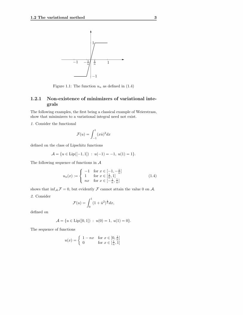
Figure 1.1: The function un as defined in (1.4)

1.2.1 Non-existence of minimizers of variational inte-

grals

The following examples, the first being a classical example of Weierstrass,show that minimizers to a variational integral need not exist.

1. Consider the functional

F(u) =

∫ 1

−1

(xu)2dx

defined on the class of Lipschitz functions

A = u ∈ Lip([−1, 1]) : u(−1) = −1, u(1) = 1.

The following sequence of functions in A

un(x) :=

−1 for x ∈ [−1,− 1n ]

1 for x ∈ [ 1n , 1]nx for x ∈ [− 1

n ,1n ]

(1.4)

shows that infA F = 0, but evidently F cannot attain the value 0 on A.

2. Consider

F(u) =

∫ 1

0

(1 + u2)14 dx,

defined on

A = u ∈ Lip([0, 1]) : u(0) = 1, u(1) = 0.

The sequence of functions

u(x) =

1− nx for x ∈ [0, 1

n ]0 for x ∈ [ 1n , 1]

4 Harmonic functions

shows that infA F = 1. On the other hand, if F(u) = 1, then u is constant,thus cannot belong to A.

3. Consider the area functional defined on the unit ball B1 ⊂ R2

F(u) =

∫

B1

√1 + |Du|2dx,

defined on

A = u ∈ Lip(B1) : u = 0 on ∂B1, u(0) = 1.

As F(u) ≥ π for every u ∈ A, the sequence of functions

u(x) =

1− n|x| for |x| ∈ [0, 1

n ]0 for |x| ∈ [ 1n , 1]

shows that infA F = π. On the other hand if F(u) = π for some u ∈ A,then u is constant, thus cannot belong to A.

1.2.2 Non-finiteness of the Dirichlet integral

We have seen that a minimizer of the Dirichlet integral is a harmonicfunction. In some sense the converse is not true: we exhibit a harmonicfunction with infinite Dirichlet integral.

The Laplacian in polar coordinates on R2 is

∆ =∂2

∂r2+

1

r

∂

∂r+

1

r2∂2

∂θ2,

and it is easily seen that rn cosnθ and rn sinnθ are harmonic functions.Now define on the unit ball B1 ⊂ R2

u(r, θ) =a02

+

∞∑

n=1

rn(an cosnθ + bn sinnθ).

Provided∞∑

n=1

(|an|+ |bn|) <∞,

the series converges uniformly, while its derivatives converge uniformly oncompact subsets of the ball, so that u belongs to C∞(B1) ∩ C0(B1) andis harmonic.

The Dirichlet integral of u is

D(u) =1

2

∫ 2π

0

dθ

∫ 1

0

(|∂ru|2 +1

r2|∂θu|2)rdr =

π

2

∞∑

n=1

n(a2n + b2n).

1.3 Some properties of harmonic functions 5

Thus, if we choose an = 0 for all n ≥ 0, bn = 0 for all n ≥ 1, with theexception of bn! = n−2, we obtain

u(r, θ) =

∞∑

n=1

rn!n−2 sin(n!θ),

and we conclude that u ∈ C∞(B1) ∩ C0(B1), it is harmonic, yet

D(u) =π

2

∞∑

n=1

n−4n! = ∞.

In fact, every function v ∈ C∞(B1)∩C0(B1) that agrees with the functionu defined above on ∂B1 has infinite Dirichlet integral.

1.3 Some properties of harmonic functions

Proposition 1.3 (Weak maximum principle) If u ∈ C2(Ω) ∩ C0(Ω)is subharmonic, then

supΩu = max

∂Ωu;

If u is superharmonic, then

infΩu = min

∂Ωu.

Proof. We prove the proposition for u subharmonic, since for a superhar-monic u it is enough to consider −u. Suppose first that ∆u > 0 in Ω. Werex0 ∈ Ω such that u(x0) = maxΩ u, we would have uxixi(x0) ≤ 0 for every1 ≤ i ≤ n. Summing over i we would obtain ∆u(x0) ≤ 0, contradiction.

For the general case ∆u ≥ 0 consider the function v(x) = u(x)+ ε|x|2.Then ∆v > 0 and, by what we have just proved, supΩ v = max∂Ω v.On theother hand, as ε→ 0, we have supΩ v → supΩ u and max∂Ω v → max∂Ω u.

Exercise 1.4 Similarly, prove the following generalization of Proposition 1.3:let u ∈ C2(Ω) ∩ C0(Ω) satisfy

n∑

α,β=1

AαβDαβu+

n∑

α=1

bαDαu ≥ 0,

where Aαβ, bα ∈ C0(Ω) and Aαβ is elliptic:∑n

α,β=1Aαβξαξβ ≥ λ|ξ|2, for some

λ > 0 and every ξ ∈ Rn. Then

supΩ

u = max∂Ω

u.

6 Harmonic functions

Remark 1.5 The continuity of the coefficients in Exercise 1.4 is neces-sary. Indeed Nadirashvili gave a counterexample to the maximum princi-ple with Aαβ elliptic and bounded, but discontinuous, see [82].

Proposition 1.6 (Comparison principle) Let u, v ∈ C2(Ω) ∩ C0(Ω)be such that u is subharmonic, v is superharmonic and u ≤ v on ∂Ω.Then u ≤ v in Ω.

Proof. Since u − v is subharmonic with u − v ≤ 0 on ∂Ω, from the weakmaximum principle, Proposition 1.3, we get u− v ≤ 0 in Ω.

Clearly

u ≤ v +max∂Ω

|u− v| on ∂Ω,

consequently:

Corollary 1.7 (Maximum estimate) Let u and v be two harmonicfunctions in Ω. Then

supΩ

|u− v| ≤ max∂Ω

|u− v|.

Corollary 1.8 (Uniqueness) Two harmonic functions on Ω that agreeon ∂Ω are equal.

Proposition 1.9 (Mean value inequalities) Suppose that u ∈ C2(Ω)is subharmonic. Then for every ball Br(x) b Ω

u(x) ≤∫

∂Br(x)

u(y)dHn−1(y), 1 (1.5)

u(x) ≤∫

Br(x)

u(y)dy. (1.6)

If u is superharmonic, the reverse inequalities hold; consequently for uharmonic equalities are true.

Proof. Let u be subharmonic. From the divergence theorem, for each

1by∫

–A f(x)dx we denote the average of f on A i.e., 1|A|

∫

A f(x)dx. Similarly∫

–AfdHn−1 = 1

Hn−1(A)

∫

AfdHn−1.

1.3 Some properties of harmonic functions 7

ρ ∈ (0, r] we have

0 ≤∫

Bρ(x)

∆u(y)dy

=

∫

∂Bρ(x)

∂u

∂ν(y)dHn−1(y)

=

∫

∂B1(0)

∂u

∂ρ(x+ ρy)ρn−1dHn−1(y)

= ρn−1 d

dρ

∫

∂B1(0)

u(x+ ρy)dHn−1(y)

= ρn−1 d

dρ

(1

ρn−1

∫

∂Bρ(x)

u(y)dHn−1(y)

)

= nωnρn−1 d

dρ

∫

∂Bρ(x)

u(y)dHn−1(y),

(1.7)

where ωn := |B1|. This implies that the last integral is non-decreasingand, since

limρ→0

∫

∂Bρ(x)

u(y)dHn−1(y) = u(x),

(1.5) follows. We leave the rest of the proof for the reader.

Corollary 1.10 (Strong maximum principle) If u ∈ C2(Ω) ∩ C0(Ω)is subharmonic (resp. superharmonic), then it cannot attain its maximum(resp. minimum) in Ω unless it is constant.

Proof. Assume u is subharmonic and let x0 ∈ Ω be such that u(x0) =supΩ u. Then the set

S := x ∈ Ω : u(x) = u(x0)

is closed because u is continuous and is open thanks to (1.6). Since Ω isconnected we have S = Ω.

Remark 1.11 If u is harmonic, the mean value inequality is also a directconsequence of the representation formula (1.11) below.

Exercise 1.12 Prove that if u ∈ C2(Ω) satisfies one of the mean value proper-ties, then it is correspondigly harmonic, subharmonic or superharmonic.

Exercise 1.13 Prove that if u ∈ C0(Ω) satisfies the mean value equality

u(x) =

∫

Br(x)

u(y)dy, ∀Br(x) ⊂ Ω

8 Harmonic functions

then u ∈ C∞(Ω) and it is harmonic.[Hint: Regularize u with a family ϕε = ρε(|x|) of mollifiers with radial simmetryand use the mean value property to prove that u ∗ ρε = u in any Ω0 b Ω for εsmall enough.]

Proposition 1.14 Consider a sequence of harmonic functions uj thatconverge locally uniformly in Ω to a function u ∈ C0(Ω). Then u isharmonic.

Proof. The mean value property is stable under uniform convergence, thusholds true for u, which is therefore harmonic thanks to Exercise 1.13.

Remark 1.15 Being harmonic is preserved under the weaker hypothesisof weak Lp convergence, 1 ≤ p <∞, or even of the convergence is the senseof distributions. This follows at once from the so-called Weyl’s lemma.

Lemma 1.16 (Weyl) A function u ∈ L1loc(Ω) is harmonic if and only if

∫

Ω

u∆ϕdx = 0, ∀ϕ ∈ C∞c (Ω).

Proof. Consider a family of radial mollifiers ρε, i.e. ρε(x) = 1εn ρ(ε

−1x),where ρ ∈ C∞(Rn) is radially symmetric, supp(ρ) ⊂ B1 and

∫B1ρ(x)dx =

1. Define uε = u ∗ ρε. Then, from the standard properties of convolutionwe find

∫

Ω

uε∆ϕdx =

∫

Ω

u(∆ϕ ∗ ρε)dx

=

∫

Ω

u∆(ϕ ∗ ρε)dx

= 0, for every ϕ ∈ C∞c (Ωε),

whereΩε := x ∈ Ω : dist(x, ∂Ω) > ε.

In particular ∆uε = 0 on Ωε. Now fix R > 0 and let 0 < ε ≤ 12R. We

have by Fubini’s theorem

∫

Ωε

|uε(y)|dy ≤∫

Ωε

1

εn

∫

Ω

ρ

( |x− y|ε

)|u(x)|dxdy

≤∫

Ω

|u(x)|dx.(1.8)

Here we may assume that u ∈ L1(Ω), since being harmonic is a localproperty. By the mean value property applied with balls of radius R

2 and(1.8), we obtain that the uε are uniformly bounded in ΩR/2. They are also

1.3 Some properties of harmonic functions 9

locally equicontinuous in ΩR because for x0 ∈ ΩR and x1, x2 ∈ BR2(x0),

still by the mean-value property,

|uε(x1)− uε(x2)| ≤ 2n

ωnRn

∫

BR2(x1)∆BR

2(x2)

|uε(x)|dx

≤ 2n

ωnRnsup

BR(x0)

|uε| ·meas(BR

2(x2)∆BR

2(x1)

),

where

BR2(x1)∆BR

2(x2) :=

(BR

2(x1)\BR

2(x2)

)∪(BR

2(x2)\BR

2(x1)

).

By Ascoli-Arzela’s theorem (Theorem 2.3 below), we can extract a se-quence uεk which converges uniformly in ΩR to a continuous function vas k → ∞ and εk → 0, which is harmonic thanks to Exercise 1.13. Butu = v almost everywhere in ΩR by the properties of convolutions, henceu is harmonic in ΩR. Letting R→ 0 we conclude.

Proposition 1.17 Given u ∈ C0(Ω), the following facts are equivalent:

(i) For every ball BR(x) b Ω we have

u(x) ≤∫

∂BR(x)

u(y)dHn−1(y);

(ii) for every ball BR(x) b Ω we have

u(x) ≤∫

BR(x)

u(y)dy;

(iii) for every x ∈ Ω, R0 > 0, there exist R ∈ (0, R0) such that BR(x) bΩ and

u(x) ≤∫

BR(x)

u(y)dy; (1.9)

(iv) for each h ∈ C0(Ω) harmonic in Ω′ b Ω with u ≤ h on ∂Ω′, we haveu ≤ h in Ω′;

(v)∫Ωu(x)∆ϕ(x)dx ≥ 0, ∀ϕ ∈ C∞

c (Ω), ϕ ≥ 0.

Proof. Clearly (i) implies (ii) and (ii) implies (iii).(iii)⇒(iv): Since h satisfies the mean value property the function w :=u− h satisfies

w(x) ≤∫

BR(x)

w(y)dy for all balls BR(x) ⊂ Ω′ s.t. (1.9) holds.

10 Harmonic functions

ThensupΩ′

w = max∂Ω′

w ≤ 0,

the first identity following exactly as in the proof of Corollary 1.10.(iv)⇒(i): Let BR(x) b Ω, and choose h harmonic in BR(x) and h = u inΩ\BR(x). This can be done by Proposition 1.24 below. Then

u(x) ≤ h(x) =

∫

∂BR(x)

hdHn−1 =

∫

∂BR(x)

udHn−1.

The equivalence of (v) to (ii) can be proved by mollifying u, compareExercise 1.13.

Often a continuous function satisfying one of the conditions in Propo-sition 1.17 is called subharmonic.

Exercise 1.18 Use Proposition 1.17 to prove the following:

1. A finite linear combination of harmonic functions is harmonic.

2. A positive finite linear combination of subharmonic (resp. superharmonic)functions is a subharmonic (resp. superharmonic) function.

3. The supremum (resp. infimum) of a finite number of subharmonic (resp.superharmonic) functions is a subharmonic (resp. superharmonic) func-tion.

Theorem 1.19 (Harnack inequality) Given a non-negative harmonicfunction u ∈ C2(Ω), for every ball B3r(x0) b Ω we have

supBr(x0)

u ≤ 3n infBr(x0)

u.

Proof. By the mean value property, Proposition 1.9, and from u ≥ 0 weget that for y1, y2 ∈ Br(x0)

u(y1) =1

ωnrn

∫

Br(y1)

udx

≤ 1

ωnrn

∫

B2r(x0)

udx

=3n

ωn(3r)n

∫

B2r(x0)

udx

≤ 3n

ωn(3r)n

∫

B3r(y2)

udx

= 3nu(y2).

1.4 Existence in general bounded domains 11

Theorem 1.20 (Liouville) A bounded harmonic function u : Rn → Ris constant.

Proof. Define m = infRn u. Then u−m ≥ 0 and by Harnack’s inequality,Theorem 1.19,

supBR

(u−m) ≤ 3n infBR

(u −m), ∀R > 0.

Letting R → ∞, the term on the right tends to 0 and we conclude thatsupRn u = m.

Proposition 1.21 Let u be harmonic (hence smooth by Exercise 1.13)and bounded in BR(x0). For r < R we may find constants c(k, n) suchthat

supBr(x0)

|∇ku| ≤ c(k, n)

(R − r)ksup

BR(x0)

|u|. (1.10)

Exercise 1.22 Prove Proposition 1.21.[Hint: First prove (1.10) for k = 1 using the mean-value identity (it might beeasier to start with the case r = R/2 and then use a covering or a scaling argu-ment). Then notice that each derivative of u is harmonic and use an inductiveprocedure.]

Proposition 1.23 Let (uk) be an equibounded sequence of harmonic func-tions in Ω, i.e. assume that supΩ |uk| ≤ c for a constant c independentof k. Then up to extracting a subsequence uk → u in C`

loc(Ω) for every `,where u is a harmonic function on Ω.

Proof. This follows easily from Proposition 1.21 and the Ascoli-Arzelatheorem (Theorem 2.3 below), with a simple covering argument.

1.4 Existence in general bounded domains

Before dealing with the existence of harmonic functions is general domainswe state a classical representation formula providing us with the solutionof the Dirichlet problem (1.1) on a ball.

12 Harmonic functions

1.4.1 Solvability of the Dirichlet problem on balls:

Poisson’s formula

Proposition 1.24 (H.A. Schwarz or S.D. Poisson) Let a ∈ Rn, r >0 and g ∈ C0(∂Br(a)) be given and define the function u by

u(x) :=

r2 − |x− a|2nωnr

∫

∂Br(a)

g(y)

|x− y|n dHn−1(y) x ∈ Br(a)

g(x) x ∈ ∂Br(a).(1.11)

Then u ∈ C∞(Br(a)) ∩ C0(Br(a)) and solves the Dirichlet problem

∆u = 0 in Br(a)u = g on ∂Br(a)

Proof. We only sketch it. By direct computation we see that u is harmonic.For the continuity on the boundary assume, without loss of generality, thata = 0 and define

K(x, y) :=r2 − |x|2

nωnr|x − y|n , x ∈ Br(0), y ∈ ∂Br(0).

One can prove that

∫

∂Br(0)

K(x, y)dHn−1(y) = 1, for every x ∈ Br(0).

Let x0 ∈ ∂Br(0) and for any ε > 0 choose δ such that |g(x) − g(x0)| < εif x ∈ ∂Br(0) ∩Bδ(x0). Then, for x ∈ Br(0) ∩Bδ/2(x0),

|u(x)− g(x0)| ≤∣∣∣∣∫

∂Br(0)

K(x, y)[g(y)− g(x0)]dHn−1(y)

∣∣∣∣

≤∫

∂Br(0)∩Bδ(x0)

K(x, y)|g(y)− g(x0)|dHn−1(y)

+

∫

∂Br(0)\Bδ(x0)

K(x, y)|g(y)− g(x0)|dHn−1(y)

≤ ε+(r2 − |x|2)rn−2

(δ2

)n 2 sup∂Br(0)

|g|.

Hence |u(x)− g(x0)| → 0 as x→ x0.

1.4.2 Perron’s method

We now present a method for solving the Dirichlet problem (1.1).

1.4 Existence in general bounded domains 13

Given an open bounded domain Ω ⊂ Rn and g ∈ C0(∂Ω) define

S− := u ∈ C2(Ω) ∩ C0(Ω) : ∆u ≥ 0 in Ω, u ≤ g on ∂Ω;

S+ := u ∈ C2(Ω) ∩C0(Ω) : ∆u ≤ 0 in Ω, u ≥ g on ∂Ω.These sets are non-empty, since g is bounded and constant functions areharmonic: u ≡ supΩ g and v ≡ infΩ g belong to S+ and S− respectively.We also observe that, by the comparison principle, v ≤ u for each v ∈ S−and u ∈ S+. We define

u∗(x) = supu∈S−

u(x), u∗(x) = infu∈S+

u(x).

and shall

1. prove that both u∗ and u∗ are harmonic;

2. find conditions on Ω in order to have u∗, u∗ ∈ C0(Ω) and u∗ = u∗ =g on ∂Ω.

This is referred to as Perron’s method.

Step 1. It is enough to prove that u∗ is harmonic in a generic ball B ⊂ Ω.Fix x0 ∈ B. By the definition of u∗ we may find a sequence vj ∈ S− suchthat vj(x0) → u∗(x0). Define

v′j := max(v1, . . . , vj) ∈ S−,

v′′j := PBv′j ,

where PBv′j is obtained by (1.11) as the harmonic extention of v′j on B

matching v′j on ∂B. Observe that by definition (v′j) is an increasing se-quence and, by the maximum principle, (v′′j ) is increasing as well. Sincethe sequence (v′′j ) is equibounded and increasing it converges locally uni-formly in B to a harmonic function h thanks to Proposition 1.23.

Observe that h ≤ u∗ and h(x0) = u∗(x0). We claim that h = u∗ in B.If h(z) < u∗(z) for some z ∈ B, choose w ∈ S− such that w(z) > h(z)and define wj = maxv′′j , w. Also define w′

j and w′′j as done before with

v′j and v′′j . Again we have that w′′j → h for some harmonic function h.

From the definition it is easy to prove that v′′j ≤ w′′j , thus h ≤ h and

h(x0) = h(x0). By the strong maximum principle, this implies h = h onall of B. This is a contradiction because

h(z) = limw′′j (z) ≥ w(z) > h(z) = h(z).

This proves that h = u∗ and then u∗ is harmonic in B, hence in all ofΩ since B was arbitrary. Clearly the same proof applies to u∗.

Step 2. The functions u∗ and u∗ need not achieve the boundary data g,and in general they don’t.

14 Harmonic functions

Definition 1.25 A point x0 ∈ ∂Ω is called regular if for every g ∈C0(∂Ω) and every ε > 0 there exist v ∈ S− and w ∈ S+ such thatg(x0)− v(x0) ≤ ε and w(x0)− g(x0) ≤ ε.

Exercise 1.26 The Dirichlet problem (1.1) has solution for every g ∈ C0(∂Ω)if and only if each point of ∂Ω is regular.[Hint: Use Perron’s method and prove that u∗ ∈ C0(Ω) and u∗ = g on ∂Ω.]

Definition 1.27 Given x0 ∈ ∂Ω, an upper barrier at x0 is a superhar-monic function b ∈ C2(Ω) ∩ C0(Ω) such that b(x0) = 0 and b > 0 onΩ\x0. We say that b is a lower barrier if −b is an upper barrier.

Proposition 1.28 Suppose that x0 ∈ Ω admits upper and lower barriers.Then x0 is a regular point.

Proof. Define M = max∂Ω |g| and, for each ε > 0, choose δ > 0 suchthat for x ∈ Ω with |x − x0| < δ we have |g(x) − g(x0)| < ε. Let b be anupper barrier and choose k > 0 such that kb(x) ≥ 2M if |x− x0| ≥ δ (bycompactness infΩ\Bδ(x0)

b > 0). Then define

w(x) := g(x0) + ε+ kb(x);

v(x) := g(x0)− ε− kb(x)

and observe that w ∈ S+ and v ∈ S−. Moreover w(x0) − g(x0) = ε andg(x0)− v(x0) = ε.

In the following proposition we see that, under suitable hypotheses onthe geometry of Ω, the existence of barriers, and therefore of a solutionto the Dirichlet problem, is guaranteed.

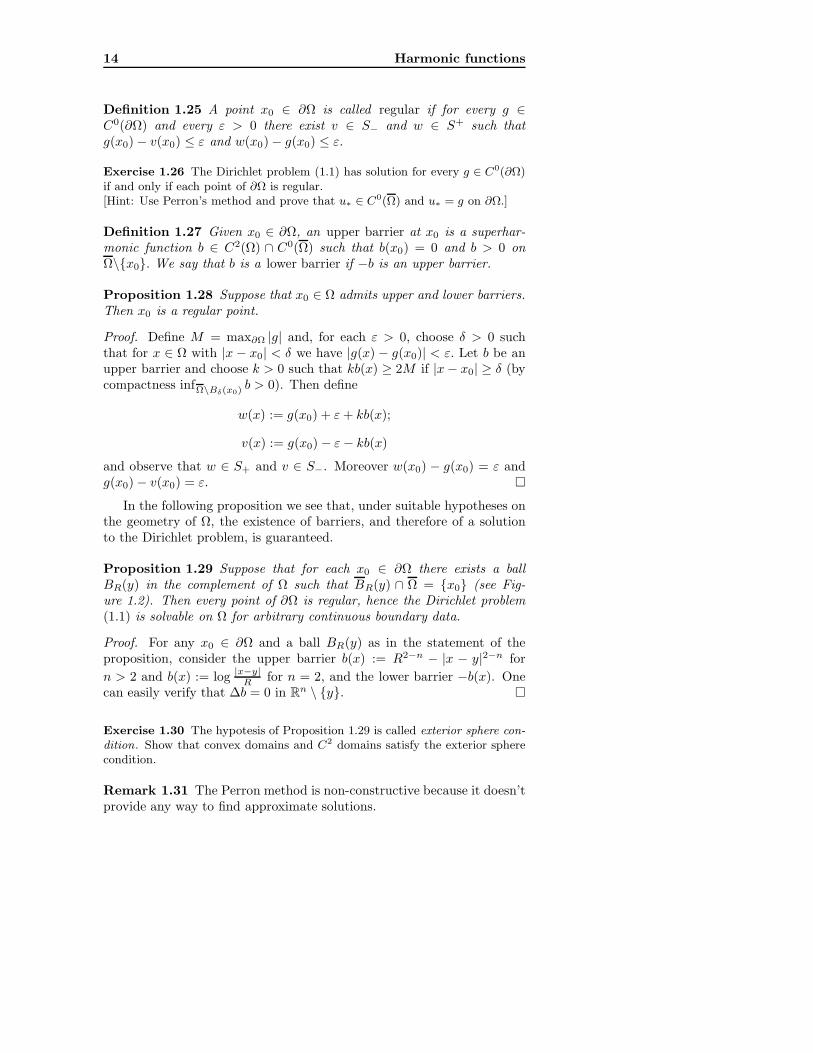
Proposition 1.29 Suppose that for each x0 ∈ ∂Ω there exists a ballBR(y) in the complement of Ω such that BR(y) ∩ Ω = x0 (see Fig-ure 1.2). Then every point of ∂Ω is regular, hence the Dirichlet problem(1.1) is solvable on Ω for arbitrary continuous boundary data.

Proof. For any x0 ∈ ∂Ω and a ball BR(y) as in the statement of theproposition, consider the upper barrier b(x) := R2−n − |x − y|2−n for

n > 2 and b(x) := log |x−y|R for n = 2, and the lower barrier −b(x). One

can easily verify that ∆b = 0 in Rn \ y.

Exercise 1.30 The hypotesis of Proposition 1.29 is called exterior sphere con-

dition. Show that convex domains and C2 domains satisfy the exterior spherecondition.

Remark 1.31 The Perron method is non-constructive because it doesn’tprovide any way to find approximate solutions.

1.4 Existence in general bounded domains 15

Ωx0

BR(y)

Figure 1.2: The exterior sphere condition.

1.4.3 Poincare’s method

We now present a different method of solving the Dirichlet problem (1.1).Cover Ω with a sequence Bi of balls, i.e. choose balls Bi ⊂ Ω, i =

1, 2, 3, . . . such that Ω =⋃∞

i=1 Bi. Now define the sequence of integers

ik = 1, 2, 1, 2, 3, 1, 2, 3, 4, . . . , 1, . . . , n, . . .

Given g ∈ C0(Ω), define the sequence (uk) by u1 := g and for k > 1

uk(x) :=

uk−1(x) for x ∈ Ω \Bik

Pikuk−1(x) for x ∈ Bik ,

where Pikuk−1 is the harmonic extention on Bik of uk−1

∣∣∂Bik

, given by

(1.11).

Proposition 1.32 If each point of ∂Ω is regular, then uk converges tothe solution u of the Dirichlet problem (1.1).

Proof. Suppose first g ∈ C0(Ω) subharmonic, meaning that it satisfiesthe properties of Proposition 1.17. We can inductively prove that uk issubharmonic and

g = u1 ≤ u2 ≤ . . . uk ≤ . . . ≤ supΩg.

Suppose indeed that uk is subharmonic (this is true for k = 1 by assump-tion). Then by the comparison principle uk+1 ≥ uk, and it is not difficultto prove that uk+1 satisfies for instance (iii) or (iv) of Proposition 1.17,hence is subharmonic.

Since, for each i, uk is harmonic in Bi for infinitely many k, increasingand uniformly bounded with respect to k, by Proposition 1.23 we see that

16 Harmonic functions

its limit u is a harmonic functions in each ball Bi, hence in Ω. Usingbarriers it is not difficult to show that u = g on the boundary.

Now suppose that g, not necessarily subharmonic, belongs to C2(Rn)and ∆g ≥ −λ. Then g0(x) = g(x) + λ

2n |x|2 is subharmonic and we maysolve the Dirichlet problem with boundary data g0. We may also solve theDirichlet problem with data λ

2n |x|2 (that is subharmonic) and by linearitywe may solve the Dirichlet problem with data g.

Finally, suppose g ∈ C0(Ω), which we can think of as continuoslyextended to Rn, and regularize it by convolution. For each convolutedfunction gε ∈ C∞(Ω) we find a harmonic map uε with uε = gε → guniformly on ∂Ω. Then by the maximum principle, for any sequenceεk → 0 we have that (uεk) is a Cauchy sequence in C0(Ω), hence ituniformly converges to a harmonic function u which equals g on ∂Ω.

Remark 1.33 The method of Poincare decreases the Dirichlet integral:

D(g) ≥ D(u2) ≥ . . . ≥ D(uk) ≥ . . . ≥ D(u).

Consequently if g has aW 1,2 extension i.e., an extension with finite Dirich-let integral, then the harmonic extension u lies in W 1,2(Ω) (for the defi-nition of W 1,2(Ω) see Section 3.2 below).

On the other hand one can also have

D(g) = D(uk) = ∞ for every k = 1, 2, . . . ,

compare section 1.2.2.

Remark 1.34 By Riemann’s mapping theorem one can show that, ifΩ ⊂ R2 is the interior of a closed Jordan curve Γ, then all boundary pointsof Ω are regular. Lebesgue has instead exhibited a Jordan domain Ω inR3 (i.e. the interior of a homeomorphic image of S2) where the problem∆u = 0 in Ω, u = g on ∂Ω cannot be solved for every g ∈ C0(∂Ω).