An Investigation into Adopting Different Piling Systems for Integral Abutment Bridges by Jitesh Harripershad Submitted in partial fulfilment of the academic requirements of Master of Science in Civil Engineering School of Engineering College of Agriculture, Engineering and Science University of KwaZulu-Natal Howard Campus South Africa March 2016
Transcript
An Investigation into Adopting Different Piling Systems
for Integral Abutment Bridges
by
Jitesh Harripershad
Submitted in partial fulfilment of the academic requirements of
Master of Science in Civil Engineering
School of Engineering
College of Agriculture, Engineering and Science
University of KwaZulu-Natal
Howard Campus
South Africa
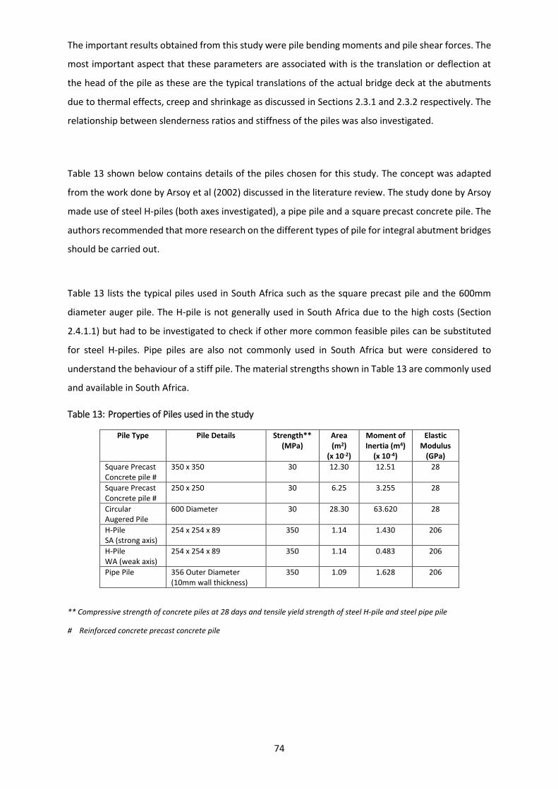
March 2016
i
PREFACE
The research contained in this dissertation was completed by the candidate while based in the
discipline of Civil Engineering, School of Engineering and of the College of Agriculture, Engineering and
Science, University of KwaZulu-Natal, Howard Campus, South Africa. The research was financially
supported by the student and eThekwini Municipality.
The contents of this work have not been submitted in any form to another university and, except where
the work of others is acknowledged in the text, the results reported are due to investigations by the
candidate.
_________________________
Signed: Supervisor - Mrs Christina McLeod
Date: 24 March 2016
ii
DECLARATION
I, Jitesh Harripershad, declare that:
(i) the research reported in this dissertation, except where otherwise indicated or
acknowledged, is my original work;
(ii) this dissertation has not been submitted in full or in part for any degree or
examination to any other university;
(iii) this dissertation does not contain other persons’ data, pictures, graphs or other
information, unless specifically acknowledged as being sourced from other persons;
(iv) this dissertation does not contain other persons’ writing, unless specifically
acknowledged as being sourced from other researchers. Where other written
sources have been quoted, then:
a) their words have been re-written but the general information attributed to
them has been referenced;
b) where their exact words have been used, their writing has been placed inside
quotation marks, and referenced;
(v) where I have used material for which publications followed, I have indicated in detail
my role in the work;
(vi) this dissertation is primarily a collection of material, prepared by myself, published as
journal articles or presented as a poster and oral presentations at conferences. In
some cases, additional material has been included;
(vii) this dissertation does not contain text, graphics or tables copied and pasted from the
Internet, unless specifically acknowledged, and the source being detailed in the
dissertation and in the References sections.
_______________________
Signed: Mr Jitesh Harripershad
Date: 24 March 2016
iii
ABSTRACT
In recent years the use of integral abutment bridges has become increasingly popular, globally. These
bridges have many advantages because the super-structure and sub-structure are monolithic in
nature, no bearings and expansion joints are required and maintenance is minimal. However these
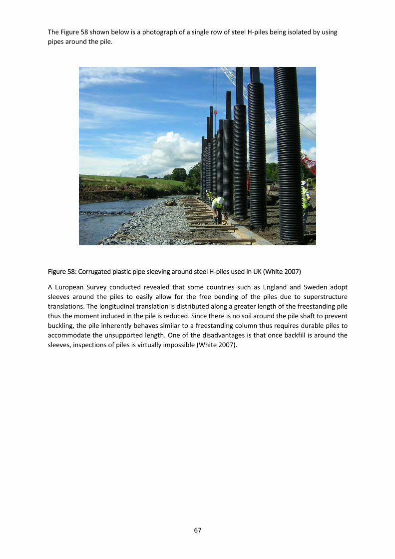
bridges are uncommon in South Africa. The behavioural performance of this type of integral structure
is influenced by the movement requirements of the foundations and steel H-piles are generally
preferred but H-piles are very rarely used in South Africa due to the high costs. This research work
investigates the behaviour and possibility of adopting other commonly used types of piles in South
Africa for integral abutment bridges instead of steel H-piles. The research also provides commonly
used techniques that are used in practice such as pile sleeving which inherently increases the
slenderness of the pile, so the pile can absorb the deck movements. Some of the common challenges
regarding integral bridges are considered and appropriate concepts are also presented. The purpose
of the research work is also to enlighten the practical bridge designer about integral abutment bridges
so important aspects are considered in the design phase. The investigation of different pile types
proposed for the integral bridge structure was based on empirical formulae and a desktop study was
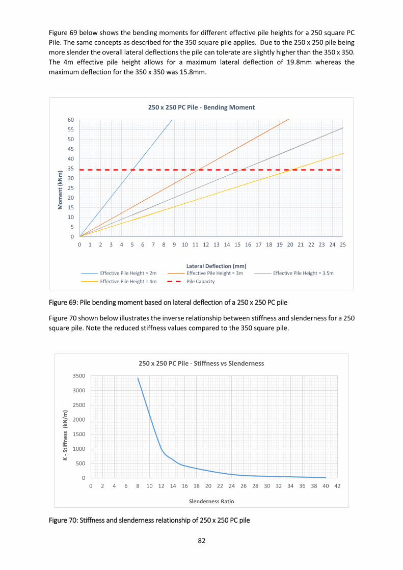
done. The outcome from the work recommends that steel H-piles on the weaker axis are a superior
choice of pile that should be used. Other pile types are also possible such as precast piles, however the
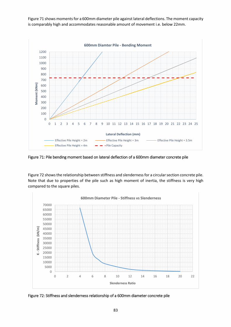
designer needs to ensure they perform well under cyclic loading. The work also recommends that a
pile sleeve or similar of over 3m long is beneficial to reduce the bending moment and shear force at
the point of virtual fixity of the pile. Integral abutment bridges have numerous advantages over
conventional bridges, however a carefully thought-out concept of the integral structure must be
considered. One important aspect is the length of the integral bridge; to ensure that the structure
performs well over its anticipated life span, integral bridges should only be used for short to medium
spans.
ix
ACKNOWLEDGMENTS
I would like to thank God, Almighty for blessing me with the strength, courage, wisdom, good
luck and guidance for helping me successfully complete my MSc dissertation and MSc course
work modules. Indeed, “God is Great”!
My sincere appreciation and thanks to my supervisor, Mrs Christina McLeod for the assistance
and positive motivation throughout this research. My gratitude is also expressed to Mr
Malcolm Jaros for his expert guidance and teachings provided in the field of foundation
engineering.
A big thank you to one of the countries bridge sages, Mr Peter G. Fenton (from eThekwini
Municipality) for also supervising, checking, brainstorming and helping me over the many
challenges faced in this research project.
I would like to express my sincere gratitude to Dan and Usha Harripershad, my father and
mother, for always providing me with the very best in my life, the loving support and the
continuous encouragement to achieve the best.
Thank you to my sister, Natisha & brother, Vikash and my friends for your inspiration and
support.
Thank you to Luke Jabulani Reid (from eThekwini Municipality) for helping with the steel
calculations, checking of the final draft, providing constructive ideas and valuable
information.
Thank you to the following helpful individuals for providing me with their time to interview
them and also for providing me with valuable information that was used in my research
project:
Mr Bruce Durrow (Royal Haskoning DHV, Pietermaritzburg)
I acknowledge eThekwini Municipality for the partial funding for my MSc post-graduate
studies.
x
TABLE OF CONTENTS
PREFACE ................................................................................................................................................... i
DECLARATION ......................................................................................................................................... ii
ABSTRACT ............................................................................................................................................... iii
ACKNOWLEDGMENTS ............................................................................................................................ ix
LIST OF FIGURES .................................................................................................................................... xii
LIST OF TABLES ...................................................................................................................................... xv
Figure 3: Temperature effect on an unrestrained element of a bridge deck (Hambly 1991) .................... 9
Figure 4: Temperature effect on a restrained element of a bridge deck (Hambly 1991) .......................... 9
Figure 5: Different type of pile cross sections (Jaradat 2005) ................................................................. 10
Figure 6: Sleeved H-piles for an integral abutment bridge (Tlustochowics 2005) ................................... 11
Figure 7: Isometric view of the integral bridge with precast prestressed piles investigated by Abendroth
et al (2007) ............................................................................................................................................ 12
Figure 8: Section of prestressed precast concrete pile adopted for the foundations for the ocean
terminal in Durban (Zakrzewski 1962) .................................................................................................... 12
Figure 9: Typical orientation of H-piles (VTrans 2009) ............................................................................ 14
Figure 10: Integral abutment details for different States :( a) Iowa DOT (Department of Transportation);
(b) Pennsylvania DOT and (c) North Dakota DOT (Burke 2009) .............................................................. 15
Figure 11- Integral abutment with CPCI girder and concrete deck - Ontario Ministry of Transportation
Figure 37: Separation of joint sealant from asphalt premix during winter (Husain et al 2000) ............... 46
Figure 38: Distinct separation of joint sealant from asphalt surface due to limits being exceeded (Husain
et al 2000) .............................................................................................................................................. 47
Figure 39: Cycle control joint type 2 – For Intermediate length bridges with light traffic - Short Integral
Abutment Bridges, Alberta guidelines for design of integral abutments (2003) ..................................... 47
Figure 40: Cycle Control Joint Type 3- For Intermediate length bridges on main highways (Alberta
2.2 The South African Bridge Loading Code – TMH7 (1988)
The current loading requirements for road bridges and culverts in South Africa are governed by
Technical Methods for Highways TMH7 (1988) Code of Practice for the Design of Highway Bridges and
Culverts in South Africa. This code was issued by the former Committee of State Road Authorities
(CSRA) and forms part of the series of Technical Methods for Highways (FitzGerald & Steyn 1998).
The TMH7 consists of three parts:
Part 1: General Statement
Part 2: Specification for Loads
Part 3: Design of Concrete Bridges
According to the current TMH7, as amended in 1988, the South African bridge code is based on limit
state design principles guided by the commendations of the CEP-FIB Model Code for Concrete
Structures published in 1978. The semi-probabilistic procedure adopts the use of partial safety factors
for determining design action effects and resistance at the ultimate limit state and the serviceability
limit state. The code is based strongly on the British code of Practice BS 5400, Parts 1, 2 and 4,
published by the British Standards Institution in 1978.
The integral bridge example used in this dissertation will adopt the TMH 7 loading regime, as amended
in 1988. The traffic loadings according to TMH 7 comprise of three independent load models NA, NB
and NC (FitzGerald & Steyn 1998).
NA Loading - represents the normal traffic loading which comprises of uniformly distributed loads
. and concentrated loads.
NB Loading - represents a single abnormal vehicle and is defined by NB 36.
NC Loading - represents super loading which refers to a multi-wheeled trailer which could have
. various combinations carrying very heavy indivisible loads.
TMH7 also covers a number of non-traffic loads. The non-traffic loads for bridges governed by TMH 7
are earth pressure, wind, hydraulics, seismic, accidental loads and thermal loads.
8
2.3 Bridge Deck Movements
Conventional design of bridges allow for the substructure and superstructure to be independent from
each other and are merely “connected”, generally by bearings and expansion joints.
Reid et al (2008) states that the expansion joint serves to join the gap and form a seal between the
two elements of a structure whilst accommodating for relative movements between them. Bridge
deck joints are specified when the bridge deck movements are quantified. There are a number of
movements to consider such as;
Temperature movements
Irreversible movements such as creep and shrinkage of the concrete
Lateral joint movements on skew decks and curved bridges
Settlement of supports
Longitudinal movements due to longitudinal forces causing a sway on the bridge from braking
and traction loads
Superstructures with deep or flexible decks are prone to significant rotation thus causing
movements under the live loads.
2.3.1 Temperature Effects
Thermal loading on bridge decks is a serviceability concern and results in flexural stresses being
developed in the concrete bridge superstructures due to the heating and cooling of concrete. The
distribution of temperature through the superstructure is nonlinear and is a function of the
superstructure depth. This can be computed by using one-dimensional heat flow analysis (Radolli &
Green 1976).
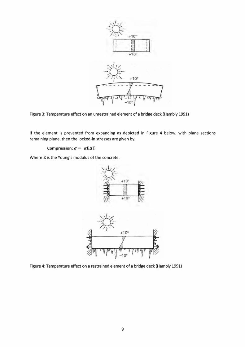
Hambly (1991) discusses how when the temperature increases in an element such as concrete, it
causes the element to expand if it is unrestrained as depicted in Figure 3. The unrestrained thermal
strains are given by;
Expansion: 𝜺 = 𝜶𝚫𝚻
Where 𝜶 is the coefficient of thermal expansion and is generally given as 12 x 10-6 oC-1 for concrete.
9
Figure 3: Temperature effect on an unrestrained element of a bridge deck (Hambly 1991)
If the element is prevented from expanding as depicted in Figure 4 below, with plane sections
remaining plane, then the locked-in stresses are given by;
Compression: 𝝈 = 𝜶𝐄𝚫𝚻
Where 𝐄 is the Young’s modulus of the concrete.
Figure 4: Temperature effect on a restrained element of a bridge deck (Hambly 1991)
10
2.3.2 Creep and Shrinkage Effects
The effects of differential creep and shrinkage in a structure is similar to that of temperature. One of
the differences is that the creep and shrinkage strain diagram is generally stepped (Hambly 1991). The
creep and shrinkage influences on integral bridges are often assumed to have opposite effects, and
are particularly difficult to evaluate accurately. Thus creep and shrinkage are often ignored in the
design of integral bridge structures (VTrans - State of Vermont Agency of Transportation, 2002).
Thippeswamy and GangaRao, as cited in a report by VTrans (2002), suggests that integral bridges with
steel or prestressed concrete girders undergoes non-uniform shrinkage through the depth of the
superstructure. The steel or prestressed concrete girders restrain the free shrinkage of the concrete
slab deck thus resulting in compressive stresses in the steel or prestressed concrete girders (at
midspan) and tensile stresses develop in the concrete deck slab.
2.4 Nature of Piles in Integral Abutment Bridges
2.4.1 Types of Piles
The research work done by Tlustochowics in 2005 discussed how there were a limited number of
published papers regarding typical pile types used in integral bridges. The research done revealed that
steel H-piles are the most commonly used pile.
The use of precast, prestressed concrete (PC) piles for integral bridges are also used by some bridge
authorities and designers such as the Iowa Department of Transportation (Abendroth et al 2007).
Research conducted by Arsoy et al (1999) stated that the main concern is the pile deflections which
arise from the cyclic movements generated from the temperature variations. Their results show that
the steel H-pile is most suitable for integral bridge abutments. Their conclusion is that further research
in this area is required. Figure 5 below shows the cross sections of various types of piles.
Figure 5: Different type of pile cross sections (Jaradat 2005)
11
2.4.1.1 Steel H-Piles
These piles have shown that they are capable of undergoing a substantial amount of distortion without
failure, thus steel H-piles are generally favoured for integral bridge applications (Burke 2009). The
research work conducted by Tlustochowics (2005) revealed that steel H-piles are able to withstand
loads induced by thermal changes (expansion and contraction effects) and so can withstand cyclic
loading provided the maximum pile stresses are within the limits of the yield stress of the pile.
Steel H-piles are manufactured in South Africa and are available but due to the cost of steel being
relatively high, they are not widely used since they are not economically viable compared to the
conventional cast insitu or precast concrete piles. (Byrne et al 1995, p89). Steel H-piles for integral
bridges are often isolated by sleeving the top few meters of the pile as shown in Figure 6.
Figure 6: Sleeved H-piles for an integral abutment bridge (Tlustochowics 2005)
2.4.1.2 Prestressed Concrete Piles
The research conducted by Abendroth et al (2007) revealed that these piles are not commonly used,
due to the concerns relating to the pile flexibility and the probability of cracking thus causing exposure
of the pre-tensioned strands to moisture and overall durability concerns. The authors discuss that
where sand and gravels are present, the use of prestressed concrete (PC) piles may be more
economical than steel H-piles. The conclusion from this research also recommends that further work
needs to be done regarding the use of PC piles for integral bridges. Figure 7 below shows an isometric
view of an integral abutment bridge with precast concrete piles.
“the available literature presents divergent conclusions regarding the
suitability of PC piles of this application”
(Abendroth et al 2007)
12
Figure 7: Isometric view of the integral bridge with precast prestressed piles investigated by Abendroth
et al (2007)
Table 1 shown below provides typical working loads for precast piles that are often used in South
Africa.
Table 1: Square precast pile working loads (Byrne et al 1995)
Pile Size 250mm Square 350mm Square
Typical working load (kN) 1000 2000
Maximum depth (m) Unlimited Unlimited
Precast pile lengths of up to 30 meters are possible by using prestressing technology but these are not
very common in South Africa (Byrne et al 1995). A typical example of the usage of prestressed piles in
South Africa are for the foundations for the ocean terminal in Durban, built in the late 1950s as shown
in Figure 8. This type of piles was predominantly used for the foundation to the jetties (Zakrzewski
1962).
Figure 8: Section of prestressed precast concrete pile adopted for the foundations for the ocean terminal in Durban (Zakrzewski 1962)
13
2.4.2 Configuration of Piles
The configuration of piles for integral abutment bridges varies in many States in the USA and generally
depends on the particular Department of Transportation guidelines.
The recommendations by the Ontario Ministry of Transportation suggest that the abutment wall
should be supported on a single row of vertical H-piles. These guidelines also advise that the end piles
at each abutment could be battered to a minimum of 1:10 in the transverse direction for additional
lateral resistance (Husain & Bagnariol 1996).
The Tennessee Department of Transportation as well as many other states recommend the use of one
row of piles driven vertically. This causes the abutment to move in the longitudinal direction, thus
increasing the degree of flexibility to accommodate for cyclic movements. (Tlustochowics 2005).
Other references such as Burke (2009) also suggest that design engineers should provide a single row
of slender vertical piles under each abutment.
2.4.3 Pile Orientation
The Ontario Ministry of Transportation recommends that if the structure’s movement and loading
requirements are such that piles are designed within the boundaries of the elastic range, then it is
suggested that the connection should be considered as fixed and the piles should be orientated such
that the strong axis is normal to the direction of the movement. When the loading and movements
are such that the pile resistance exceeds the elastic range, the connection should be assumed as
pinned and the piles weak axis orientated such that they are normal to the direction of movement
(Husain & Bagnariol 1996).
According to Burke (2009), suggests that engineers generally orientate the
“weak axis of H-piles normal to the direction of pile flexure”.
The literature review by Tlustochowics (2005) revealed that various States in the USA have different
opinion and practice regarding pile orientation for integral abutment bridges. The work reveals that
according to a survey done in 1983, fifteen states in the USA orientate the piles so that the direction
of thermal movement causes bending actions about the strong axis of the pile whilst thirteen other
states orientate the piles such that the direction of movement causes bending about the weak axis of
the pile. The piles orientated such that bending is about the strong axis is due to perhaps some degree
of stiffness required to carry supplementary loads such as skidding and braking forces on the deck.
The research also discussed that the most common recommendation is to orientate piles such that
bending is about the weak axis of the pile. According to the research for stub abutments the pile axis
of bending has a negligible effect regarding the displacement capacity for integral stub abutments.
14
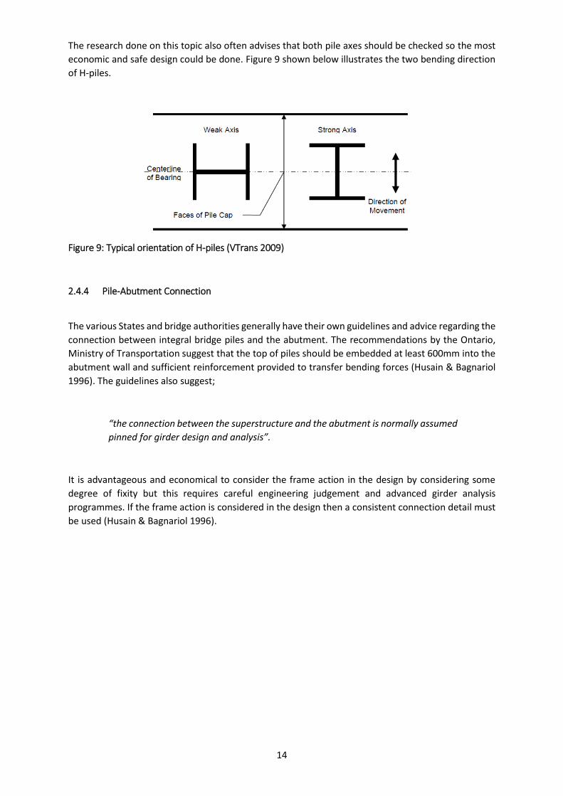
The research done on this topic also often advises that both pile axes should be checked so the most
economic and safe design could be done. Figure 9 shown below illustrates the two bending direction
of H-piles.
Figure 9: Typical orientation of H-piles (VTrans 2009)
2.4.4 Pile-Abutment Connection
The various States and bridge authorities generally have their own guidelines and advice regarding the
connection between integral bridge piles and the abutment. The recommendations by the Ontario,
Ministry of Transportation suggest that the top of piles should be embedded at least 600mm into the
abutment wall and sufficient reinforcement provided to transfer bending forces (Husain & Bagnariol
1996). The guidelines also suggest;
“the connection between the superstructure and the abutment is normally assumed
pinned for girder design and analysis”.
It is advantageous and economical to consider the frame action in the design by considering some
degree of fixity but this requires careful engineering judgement and advanced girder analysis
programmes. If the frame action is considered in the design then a consistent connection detail must
be used (Husain & Bagnariol 1996).
15
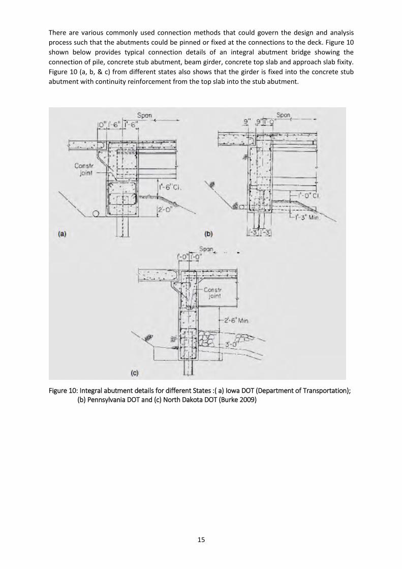
There are various commonly used connection methods that could govern the design and analysis
process such that the abutments could be pinned or fixed at the connections to the deck. Figure 10
shown below provides typical connection details of an integral abutment bridge showing the
connection of pile, concrete stub abutment, beam girder, concrete top slab and approach slab fixity.
Figure 10 (a, b, & c) from different states also shows that the girder is fixed into the concrete stub
abutment with continuity reinforcement from the top slab into the stub abutment.
Figure 10: Integral abutment details for different States :( a) Iowa DOT (Department of Transportation); (b) Pennsylvania DOT and (c) North Dakota DOT (Burke 2009)
16
Using a rubber bearing under the girder creates a “pinned” condition to a certain extent and is
contentious. The rubber bearing will be permanently fixed and would be impossible to replace as
shown in the Figure 11 below. Figure 11 also shows the 600mm pile embedment into the concrete
stub abutment. The stub abutment concept is very common with integral bridges as they essentially
reduce the potential active and passive soil pressures behind the wall. This abutment concept also
allows greater flexibility rather than a high abutment wall which generally has to be stiffened by
counterforts.
Figure 11- Integral abutment with CPCI girder and concrete deck - Ontario Ministry of Transportation (Husain & Bagnariol 1996)
17
Figure 12 shown below is similar to the concept presented in Figure 11. To create the pinned
connection at deck and abutment interface a continuous strip of thin rubber bearing is placed under
each girder as shown.
Figure 12: Integral abutment with precast concrete box girder and concrete deck - Ontario Ministry of Transportation (Husain & Bagnariol 1996)
The research and testing done by Abendroth et al (2007) adopted the use of “carpet wrap” at the top
ends of the prestressed concrete piles supporting the abutment as shown in Figure 13. The carpet rap
is a padding material that is installed (wrapped) around the pile that is embedded in the concrete stub
abutment. The aim of this was to reduce rotational restraint at the tops of the abutment piles and
create conditions of a “pinned type connection” between the piles and abutment. Carpet wrap is
common practice and is often used in such applications. The results from the pile strain data did not
reveal how much freedom of rotation was available for this type of connection and the researchers
suggested that carpet wrapping at the top of piles should not be assumed to be a fully pinned-end
condition.
Figure 13: Precast PC pile wrapping detail for the research done by Abendroth et al (2007)
18
2.4.5 Length and Skew Limits for Integral Bridges
2.4.5.1 Length Limitations
The length limit is an important consideration in the design of integral bridges. Some of the
recommended lengths are discussed below. Table 2 below summarises the length limits for integral
steel and concrete bridges used in various states.
Table 2: Recommended maximum length limits for Integral Bridges (Tlustochowics 2005)
Department/state of Transportation
Concrete Integral Bridge length
(m)
Steel Integral Bridge length
(m)
Colorado 240 195
Illinois 125 95
New Jersey 140 140
Ontario, Canada 100 100
Tennessee 244 152
Washington 107 91
The literature review conducted by Card & Carder (1993) revealed that composite (steel-concrete)
bridges undergo about 20% greater movement ranges in effective bridge temperature than concrete
decks whilst steel box girders could experience 50% greater movement ranges. The table 2 above,
thus shows smaller bridge lengths for steel integral bridges than concrete integral bridges. The table
also shows that there is no common limit for integral bridge lengths as there is high variation in the
values presented in the table.
The Ontario Ministry of Transportation suggests where the overall length of a bridge structure is over
100m but less than 150m, it may be designed as an integral bridge (Husain & Bagnariol 1996). The
Design Manual for Roads and Bridges – The Design of Integral Bridges (BA 42/96) suggests that bridge
decks of up to 60m in length are generally required to be designed as an integral bridge. In Switzerland
the largest possible concrete integral bridge length is 108m, this transpires from national codes and
based on the limitations of accepted deformations (Dreier et al 2010).
The Tennessee Department of Transport (DOT) is generally leading in integral bridge development.
For example, The Happy Hollow Creek Bridge is a seven span prestressed concrete curved integral
bridge with a total length of over 358m as shown in Figure 14. A single row of steel H-piles were used
to support each abutment (Burke, 2009).
19
Figure 14: Aerial view of Happy Hollow Creek Bridge (Burke 2009)
The research by Tlustochowics (2005) discusses how as the integral bridge length increases, the lateral
cyclic displacements in the piles due to temperature variations also increase. The piles may not
perform within their elastic limits and may deform within the plastic range resulting in a reduction in
their service life.
2.4.5.2 Skew Limitations
The Ontario, Ministry of Transportation suggests that if a rigorous analysis is carried out to account
for skew effects, skews greater than 20o but not exceeding 35o may be considered. The reasons for
the limitation on skew are primarily due to the non-uniform distribution of loads and complexities in
establishing the movements in its associated direction (Husain & Bagnariol 1996). The Design Manual
for Roads and Bridges – The Design of Integral Bridges (BA 42/96) advocates that integral bridge skews
should not exceed 30o.
The Project Report by Card and Carder (1993) recommends that the skew angle for integral bridge
abutments should be minimised, usually between 10o to 15o but typically not greater than 30o. The
research also discusses how skews are limited to minimise the pile deflection in both longitudinal and
transverse planes. When the skews are large, raked piles have been used to resist rotation caused by
the earth pressures.
Figure 15 below shows the bridge length and skew limits for integral, semi-integral and conventional
abutment designs. Figure 15 shows that for an integral abutment bridge the length limit is 61m and
the maximum skew angle permitted is 30o as per the literature. The semi-integral abutment bridges is
permitted to have lengths up to 125m and thereafter conventional abutment design is governed for
higher lengths.
20
Figure 15: Skew angle limitations of Integral and Semi-Integral abutment bridges versus bridge length (Ohio, Department of Transportation 2003)
2.5 Chapter Summary
The main aim of this chapter was to understand the benefits of adopting integral abutment bridges.
This chapter introduced the various fundamental requirements for integral abutment bridges. The
numerous advantages of integral bridges are coupled with limitations such as the length and skew
limits. The literature review showed there exists a wide spectrum regarding the integral bridge length
limit and varies in different states. The types of piles were described and details provided; the steel H-
pile is the preferred choice according to the literature reviewed. The soil-structure interaction is
perhaps the biggest challenge concerning integral abutment bridges and is discussed in the
forthcoming chapter.
21
CHAPTER 3
3 ISSUES CONCERNING INTEGRAL BRIDGE ABUTMENTS
3.1 Design Methods
3.1.1 General Issue
Integral bridges have numerous advantages, however the main difficulty from a designer’s perspective
is the soil-structure interaction. The interaction between abutment walls, supporting piles and soil
media are essential for the analysis and understanding the structural behaviour (David & Forth 2011).
A commonly used modelling method is to postulate a series of spring supports along the foundation
piles and behind the abutment walls. The main challenge with the spring type model is the derivation
of the spring constant. Ideally the aim is to simulate actual site conditions (Sisk & Terzaghi, 2009).
3.1.2 Calculation Methods
There are several methods and models for analysing integral abutments. One of the most common
methods is by adopting complex finite element models. However such detailed analysis is seldom
adopted in practice as most states apply the simple length and skew rules with their typical state
designed details. Research conducted at the Iowa State University has led to two fundamental types
of equivalent cantilever pile analysis alternatives, one for elastic stresses and a second that considers
plastic stress (Dunker & Liu 2007).
According to David and Forth (2011), there are six modelling approaches generally adopted by
researchers for analysis of soil structure interactions;
I. Winkler spring approach
II. Finite element analysis
III. Integrated modelling
IV. Partitioned analysis
V. Staggered approach and
VI. Iterative coupling
Some of the common methods and models are briefly discussed below.
22
3.1.2.1 Equivalent Cantilever Method
The equivalent cantilever method is a simplified model presented by Abendroth and Greimann in the
late 1980s. The pile and surrounding soil is modelled as a column with a fixed base at some distance
below the ground surface. This method is based on finite element and analytical studies and can
consider the elastic or plastic behaviour of piles. Both these alternatives are conservative when
compared to finite element simulations. The concept is illustrated in the Figure 16 and Figure 17
shown below. However this method does not simulate the abutment wall and approach fill interaction
In 1948 Palmer and Thompson presented the commonly used formulae below;
𝐤𝐡 = 𝐤𝑳 (𝐳
𝐋)
𝐧
Where:
z = depth below surface
L = length of pile
𝐤𝑳 = is the value of 𝐤𝐡 at the pile tip (z = L)
n = an empirical index equal to or greater than zero
A common assumption is that 𝑛 = 0 for clay. This implies that the spring constant is same throughout
the pile. Another assumption is that 𝑛 = 1 for granular soils, thus the modulus increases linearly with
depth. In 1963, Davisson and Prakash suggested that for clays a more realistic value to consider for
undrained conditions will be 𝑛 = 0.15. The undrained conditions are considered since the clay
particles are surrounded by a nearly incompressible layer of fluid such as water.
For the case of 𝑛 = 1;
𝐤𝐡 = 𝐧𝒉 (𝐳
𝐝)
.
Where:
𝐧𝒉 = coefficient of subgrade reaction (units of force/ length3)
d = pile width or diameter
28
The true behaviour of soils is such that soil pressure and deflection are non-linear, with soil pressure
approaching a limited value when deformations are high. The range of limiting values is essentially
based on the soil type. The p-y approach developed by Reese may be the most satisfactory method to
carry out a non-linear analysis. If linear theory is to be adopted then appropriate secant values of the
subgrade modulus must be chosen (Poulos & Davis 1980). However the work done by Tlustochowicz
(2005) also states that the formulae by Palmer and Thompson proposed in 1948 is widely used. The
work done by Tlustochowicz (2005) as shown in Table 3 below, summarises proposed coefficients of
reactions by Davisson in 1970. Table 3 provides subgrade reaction modulus ranges for the different
soil types. For cohesive soils the subgrade reaction modulus is dependent on the undrained shear
strength of the soil.
Table 3: Estimated values of coefficient of subgrade reaction modulus (Davisson 1970 cited by Tlustochowics 2005)
Rombach (2011) suggested that rigid piles can be modelled by linear elastic supported truss elements.
The bedding modulus 𝒌s and the stiffness of horizontal springs around the pile shaft may vary along
its length and circumference. The Figure 23 shown below illustrates this concept. The work done
presents a proposed method by Timm and Bladauf (1988) which suggests the formulae below;
𝒌𝒔(𝒛) = 𝒌𝒔(𝒅). (𝒛
𝒅)
𝒏
Where:
𝑛 = 0 for cohesive soils under small loads, similar to Palmer and Thompson (1948)
𝑛 = 0.5 for medium cohesive soil and non-cohesive soil above ground water table
𝑛 = 1.0 for non-cohesive soil below the ground water level or under greater loads
𝑛 = 1.5 𝑡𝑜 2.0 for loose non-cohesive soil under very high loads.
Figure 23: Distribution of bedding modulus ks and numerical model for a laterally loaded pile (Rombach 2011)
29
Rombach (2011) recommends that if no results are available from actual pile tests then the bedding
modulus 𝒌s may be estimated from the following expression;
𝒌s = 𝑬s/𝒅
Where:
𝒌s is the bedding modulus
𝑬s is the stiffness modulus of the ground
𝒅 is the diameter of the pile where d is less than or equal to 1000 mm
Further guidelines provided suggest that the stiffness modulus for non-cohesive soil varies between
𝑬s = 100 to 200 MN/m2 for gravel whilst 𝑬s varies between 10 to 100 MN/m2 for sand (Rombach 2011).
The modulus of subgrade reaction has also been proposed by various other researchers and some of
them are discussed below.
Terzaghi in 1955 proposed that the modulus for subgrade reaction is the same horizontally and
vertically for clays and is actually independent of depth. Typical values for the over-consolidated clays
are show in the Table 4 below;
Table 4: Values of ksl (tons/ft3) for square plates, 1 x 1 ft., on overconsolidated clays (Terzaghi 1955 cited in Poulos & Davis 1980)
Vesic (1961) compared results from an infinite horizontal beam on elastic foundation to results
obtained from subgrade reaction theory and found the following relationship;
𝒌 = (𝟎. 𝟔𝟓
𝒅) √
𝑬𝑺𝒅𝟒
𝑬𝑷𝑰𝑷
𝟏𝟐
(𝑬𝑺
𝟏 − 𝝂𝑺𝟐)
Where:
𝑬𝑷𝑰𝑷 = pile stiffness
𝒅 = pile diameter
Broms (1964) proposed the empirical correlation, that 𝒌h for clays is related to the secant modulus
𝑬50 at half the ultimate stress in an undrained test;
𝒌𝒉 = 1.67.𝑬𝟓𝟎/d
30
Whilst Skempton (1951) suggested using an 𝑬𝟓𝟎 value equal to 50 to 200 times the undrained shear
strength, 𝒄𝒖 thus obtaining the relationship;
𝒌𝒉 = (𝟖𝟎 − 𝟑𝟐𝟎)𝒄𝒖/𝒅
A more conservative reaction of subgrade modulus was suggested by Davisson (1950);
𝒌𝒉 = 𝟔𝟕𝒄𝒖/𝒅
Although many researchers propose that for clay, the 𝒌𝒉 value could be considered constant along
the length of a pile shaft, some researches assume that 𝒌𝒉 increases linearly with depth;
𝒌𝒉 = 𝒏𝒉. (𝒛
𝒅)
Typical values are presented in Table 5 below;
Table 5: Typical values for 𝒏𝒉 in cohesive soils (Davis & Poulos 1980)
For sands, Terzaghi (1955) assumed that the modulus of elasticity depends on the density of the sand
and overburden pressure thus found the following correlation;
𝒏𝒉 = 𝑨. 𝜸
𝟏. 𝟑𝟓 (𝒕𝒐𝒏𝒔/(𝒇𝒕𝟑 )
Typical values of 𝑨 and 𝒏𝒉 are shown in the Table 6 below;
Table 6: Values of 𝒏𝒉 (ton/ft3) for sand (Terzaghi 1955 cited in Davis & Poulos 1980)
31
Research by Sisk and Terzaghi (2009) suggests that different methods for obtaining the spring
constants along a pile give widely varying results, which could lead to over or under designing the
piles. The use of conventional springs is thus discouraged and the combining of the structural
geotechnical models is promoted.
3.2.3 Laterally Loaded Piles
Research work done by Broms (1965) suggested that the ultimate lateral resistance of a laterally
loaded pile is governed by;
I. The ultimate lateral resistance of soil surrounding the pile
II. The moment resistance of the pile section
The ultimate lateral resistance of piles can be calculated from graphs that were presented by Broms
(1965). The work carried out showed that for short piles, the ultimate lateral resistance was
dependent on the depth of the pile and independent of the resistance offered by the pile section. The
ultimate lateral resistance for a long pile was found to be governed by the ultimate lateral resistance
of the pile section and independent of the pile penetration depth.
The method presented by Broms (1965) was based on the concept of a coefficient of subgrade
reaction and assumed that for cohesion-less soils, it increases linearly with depth whilst for cohesive
soils it remains constant with depth. When plastic hinges develop along the length of a steel, timber
or reinforced concrete pile, collapse occurs as a form of failure mechanism. Broms (1965) assumed
that the rotational capacity of these plastic hinges is enough to develop the passive lateral soil
resistance, allowing full redistribution of bending moments along the length of the piles.
Local buckling may occur for relatively thin walled pipe piles. In this case, Broms’ (1965) proposed
analysis would not apply. It is suggested that the local buckling can be easily prevented if the steel
pipe piles are filled with sand or concrete. The wall thickness of pipe piles as well as the web and
flange thickness of H-pile sections should be chosen such that local buckling does not occur, generally
local buckling is not likely to occur if conventional sections are adopted. When the stress at the
sections of maximum bending moment reaches the yield strength of the pile material, plastic hinges
are formed in steel piles. The plastic moment of resistance of the section, 𝑴𝒚𝒊𝒆𝒍𝒅 can be calculated
based on ultimate strength analysis.
For a cylindrical steel pipe section;
𝑴𝒚𝒊𝒆𝒍𝒅 = 𝟏. 𝟑𝒇𝒚𝑾
And for an H- section pile;
𝑴𝒚𝒊𝒆𝒍𝒅 = 𝟏. 𝟏𝒇𝒚𝑾𝒎𝒂𝒙
32
Where:
𝒇𝒚 is yield strength of pile material
𝑾 is section modulus of the pile
And coefficients of 1.3 and 1.1 are plastic moment shape factors for the respective sections.
It is important to note that in the literature presented by Broms (1965), the axial loads that are likely
to be present in reality are now ignored because axial loads decrease the ultimate bending resistance
strength of steel H-piles and pipe piles, whilst in the case of precast and cast in-situ piles it is increased.
The reason for such behaviour depends on the type of material and the degree of buckling resistance
provided, which essentially depends on the buckling mode of failure.
The Figure 24 and Figure 25 shows the soil reaction and bending moment of short piles in cohesive
and cohesionless soil respectively.
Figure 24: Cohesive soil – short pile under horizontal loads (Broms 1964 cited in Tomlinson 1994)
Figure 25: Cohesionless soil – short pile under horizontal loads (Broms 1964 cited in Tomlinson 1994)
33
The Figure 26 and Figure 27 shows the soil reaction and bending moment of long piles in cohesive
and cohesionless soil respectively.
Figure 26: Cohesive soil – long pile under horizontal loads (Broms 1964 cited in Tomlinson 1994)
Figure 27: Cohesionless soil – long pile under horizontal loads (Broms 1964 cited in Tomlinson 1994)
34
3.3 Geotechnical Problems and Solutions Using Materials to Absorb Lateral Stresses Behind Integral
Bridge Abutments
3.3.1 General Overview
Integral bridge abutment concept has many advantages as previously discussed but as historically
implemented can have its own inherent post-construction flaws. The problems are fundamentally of
a geotechnical nature and not structural. Thus, for an improved and better long-term performance of
an integral bridge, it is imperative the designer considers the soil-structure interaction of the bridge
abutments (Horvath 2005). One of the fundamental flaws of integral abutment bridges is that the
concept fails to demonstrate how the relative displacement between the cyclic movement of the
superstructure (and /or substructure) and ground is to be accommodated. This has actually led to
integral bridge abutments still requiring maintenance when in actual service, although many authors
argue that the cost for this maintenance is less than that for conventional bridges with joints and
bearings (Horvath 2005).
3.3.2 Thermal Effects on Integral Abutment Bridges
“Thus IABs (integral abutment bridges) as currently designed still have
maintenance costs as did their jointed predecessors which inflates the true life-
cycle cost of an IAB”
(Horvath 2005)
Figure 28 below describes the abutment behaviour of an integral bridge. As Horvath describes, the
abutment primarily undergoes rigid-body rotation about the bottom of the abutment but there is also
a certain degree of rigid-body translation of the abutment. Since rotation of the abutment is dominant,
the magnitude of the horizontal displacement at the top will be greatest.
Due to seasonal temperature changes, the bridge superstructure experiences corresponding seasonal
length changes, i.e,
i. In winter the integral abutments move inwards and away from the soil mass they are
retaining.
ii. In summer the integral abutments move outward and push into the soil mass
The magnitude of these thermal movements depend on the length of bridge, coefficient of thermal
expansion of material and the corresponding temperature range as discussed in Chapter 2 (2.3.1).
Figure 28: Thermal effects on Integral Abutment Bridges and Displacements (Horvath 2005)
35
Horvath (2005) explains that as a result of the cyclic behaviour, at the end of each annual thermal
cycle, there is often a net displacement of each abutment inwards toward each other and away from
the retained soil mass as shown in Figure 28. This inward displacement of the abutment as a result of
the winter season is of sufficient magnitude to cause active earth pressure conditions behind the wall
thus resulting in a “soil wedge” to develop adjacent to each abutment and follow the abutment wall
inwards, with the soil slumping downwards behind the abutment wall. Since the soil is inelastic in
nature, the inward and downward movement of the soil mass is not fully recovered during the summer
season when the abutment is pushed outwards. The author also emphasises that this inward and
downward displacement of the soil will occur, irrespective of the type of soil and degree of compaction
adopted during construction. One should also note that, the net inward movement of the abutment
is intensified when the superstructure is concrete due to the inherent shrinkage of concrete. There
are two significant consequences that result from the seasonal thermal effects
3.3.2.1 Ratcheting Failure
The first was discovered as early in the 1960s (Broms 1971, Card 1993 & Sandford 1993 cited in
Horvath 2005) and is the relatively large lateral earth pressures that develop on the abutment wall
during the annual summer expansion of the superstructure. These lateral earth pressures can
approach the theoretical passive pressure especially towards the upper part of the abutment where
horizontal displacements are generally the greatest. If the abutments are not designed for these high
pressures, structural distress and even failure of an abutment can occur. The summer-seasonal
increase in lateral earth pressure, which is not necessarily constant over time, can increase
significantly.
“The reason is that not only is one seasonal cycle of inward-outward
displacement nonlinear, but each succeeding season is nonlinear with
respect to the proceeding one.”
(Horvath 2005)
In simple terms, this implies that each winter the abutment moves slightly inward more than the
preceding winter and each summer it moves slightly outwards to a lesser degree than the preceding
summer. There is a “consistent” net soil displacement inward towards the abutments yet the bridge
superstructure still expands each summer season the same amount as the preceding year. As a result,
the lateral earth pressures increase over the summer season as the soil mass directly behind the
abutment wall becomes increasingly wedged in over many cycles. This complex overall soil mechanics
behaviour is termed ratcheting (Horvath 2005).
The ratcheting effect results in each summer’s lateral earth pressures being higher in magnitude than
those of the preceding year. This essentially implies that structural distress at abutments and failure
of the abutments are likely after a few decades or even years, and represents a potentially serious
“long-term” problem for integral bridge abutments. This also implies that the full design service life of
the bridge may not be achieved (Horvath 2005).
36
3.3.2.2 Void Subsidence
The second significant problem associated with integral abutment bridges is the void that develops
behind the abutment face as illustrated in the figure 29 below;
Figure 29: Subsidence of the ground surface behind integral abutment bridges (Horvath 2005)
Due to the irreversible slumping of the soil-wedge behind each abutment, a subsidence pattern forms
adjacent to each abutment as shown in Figure 29. This subsidence pattern is also a result of the overall
net inward displacement of the abutment. The subsidence pattern (gap) depends on whether or not
a transition slab (approach slab) was constructed as part of the abutment. If no approach slab is used,
there will be a difference in road surface elevation over a short distance, creating the typical “bump”
at the end of the bridge. If a transition slab is adopted, then it will initially span over the gap/void
created underneath by the subsided soil mass (Horvath 2005). The research by Reid, as cited by
Horvath (2005) reveals that from a field survey of 140 IAB’s (integral abutment bridges) approach slabs
in the state of South Dakota, USA, a void was found under practically every approach slab, the void
depths varied from 13mm to 360mm and the void length under the approach slab extended as much
as 3m.
3.3.3 Proposed Solutions Using Stress Absorbing Materials
Recent work related to finding solutions to some of the problems with regard to integral bridge
abutments include the study of different types of compressible materials. In concept these
compressible materials are intended to serve as a sacrificial cushion between the abutment and
adjacent soil mass thus reducing the lateral earth pressures caused by seasonal thermal movements
(Horvath, 2005).
“Because of the current extensive use of IABs, there is a critical need to
develop solutions to correct the behavioural deficiencies inherent in all IABs
as they are typically designed and constructed at the present time”
(Horvath, 2005)
37
Horvath (2005) based solutions on the following considerations and concepts;
I. The natural phenomenon of expansion and contraction of the bridge superstructure due to
seasonal temperature variation is inevitable and unavoidable and the displacement will
occur regardless of concept adopted in the design phase. The displacement between the IAB
and soil mass is thus unavoidable and must be addressed in the design.
II. Horvath also suggests the soil mass behind the IAB abutment must be made “inherently self-
stable” for all seasonal cycles thus preventing the development of subsidence (gap) during
the winter seasons.
III. A specialised material or structural element (compressible layer) must be provided between
the “inherently self-stable” soil mass and the moving IAB concrete abutment to reliably
accommodate for the horizontal displacement between them. In the past voids have been
left between the ground and abutment but experience has shown that this is difficult to
construct and the reliability of the gap for long term effects is uncertain.
Horvath (2005) presents two different concepts, the details are provided below and illustrated in
Figure 30.
Concept 1: (as shown in Figure 30(a))
The concept makes use of geosynthetic tensile reinforcement to create a mechanical stabilised earth
(MSE) mass behind the concrete abutment thus achieving an “inherently self-stable” soil mass for the
design life of the bridge.
Figure 30(a) below is most likely to be cost effective and appropriate in most conditions with some of
the key features:
Figure (a) below is appropriate were the insitu soils have no issues regarding compressibility
or stability
A relatively thin (typically in the order of 150mm) layer of compressible material such as
resilient- EPS (expanded polystyrene) geofoam would be adopted to serve as a compressible
inclusion between the soil mass and abutment wall.
The durable compressible material functions as the desired “expansion joint” between the
concrete abutment and MSE soil mass.
The compressible material layer also thermally insulates the retained soil from winter
freezing and insulates the geosynthetic tensile reinforcement from the summer heat which
can increase the geosynthetic creep.
The compressible inclusion can also be designed to serve as a drain for ground water flow.
The most important function of the compressible inclusion layer is to allow the
reinforcement within the soil mass to strain in tension thus preventing the soil from moving
inwards towards the abutment back-face and downwards during each winter season. In
addition it allows the abutments to move seasonally (expanding and contracting) either way
with minimal restraint. In summer seasons the lateral earth pressures are reduced to
relatively smaller magnitudes, this advantage could result in cost savings for the structural
design of the abutment.
38
Concept 2: (as shown in Figure 30(b))
The other alternative is shown Figure 30(b) below, some of the features of this proposal are listed
below;
As an alternative to the MSE soil mass, one could adopt a self-stable wedge of geofoam such
as EPS blocks.
The use of lightweight fill material also has many advantages such as reducing the loads
imposed onto the abutment and the underlying ground layers. This alternative is thus
appropriate for sites where the insitu soils underlying the approach embankment are
compressible and soft.
The compressible material forming the inclusion serves the same purpose as described
above.
Figure 30: Schematic Proposal of New IAB Design Alternatives by Horvath (2005)
The new IAB design alternatives, as shown in Figure 30 above, aims to isolate the structure from the
surrounding soil mass and simplify the complex soil-structure interaction. The scheme shown in Figure
30(a) would be more practical for construction in South Africa as the concept of using geosynthetic
tensile reinforcement or similar material in mechanically stabilized earth retaining walls is popular,
with the resources and expertise for such an application readily available.
SUMMARY OF RESEARCH WORK BY CARDER, BARKER & DARLEY (2002)
Stress-absorbing layers between the backfill and abutment by use of various innovative materials have
been identified and a testing regime was set up to primarily assess their fitness for purpose. The
authors above selected a product from each generic type of material and set up a testing programme.
The testing programme was aimed at investigating;
I. Potential fitness for purpose of a specific type of material and
II. Refine the testing procedures
39
The test procedures proposed included;
I. Determination of modulus at strain levels expected in the field
II. Shear strength
III. Permanent compression set, locked-in when the loading applied was released
IV. Thereafter actual trials were undertaken to assess the effect of compacting granular
fill against some of the materials
The suitably identified materials investigated were;
I. Polyethylene foam
II. Expanded polystyrene
III. Extruded polystyrene
IV. Geocomposite
V. Voided rubber
VI. Rubber-soils
VII. Shredded tyres
VIII. Rubber crumb
The results of the investigation showed that some of the materials prove to have good potential for
use as layers to absorb lateral stresses behind the IAB concrete abutment. The main concern was that
some materials exhibited a compression set on the release of the load. This phenomenon in practice
would result in excessive void formation when subjected to cyclic loading. The solution that the
authors proposed was to adopt thicker material layers to limit the in-service strains and thus in turn
reduce the compression set.
The tests were in accordance with the recommended engineering properties of the stress-absorbing
layer behind an integral bridge abutment published by Carder and Card (1997). The properties were
derived on the basis of typical requirements for a continuous deck with the following properties;
I. Deck span of 60m. Note 60m is also the limit of integral bridge length in many states in the
USA.
II. Assuming a coefficient of thermal expansion of 12 x 10-6 per oC.
III. The effective deck temperature range was based on that which is experienced in the United
Kingdom (UK).
The figures below are a typical example of the results obtained from tests performed on the expanded
polystyrene. Similar tests were performed on the other type of materials. The figure below shows the
results from compression testing to determine the horizontal modulus. The figures show typical stress-
strain plots on compression of expanded polystyrene at strain limits of 2% and 6% in Figure 31 and
Figure 32 respectively. From these tests performed by the researchers, the tangent modulus values
were obtained from a series of three tests and are tabulated next to the figures. These values were
determined after accommodating for initial seating effects due to friction between the specimen sides
and the box used for testing. From Figure 31 the expanded polystyrene proved to be elastic in nature
up to approximately 2% of strain, yielding a mean modulus of 6.6 MPa for the first loading. Due to
effects of the specimen being confined in the test box, the values were higher than the manufacturer’s
conservative value of 4.5 MPa.
40
Figure 31: Modulus testing of expanded polystyrene (first load cycle of 2% strain) – (Carder et al 2002)
In Figure 32 shown below, testing up to 6% strain was carried out on the expanded polystyrene. A
small change in the modulus was measured but significant plastic deformation was observed when
the strains above 2% occurred. A distinct increase in permanent deformation was recorded after
unloading was done. This indicated that the need to control the working strain of expanded
polystyrene to less than 2% was required if it were to be adopted behind integral bridge abutments
to avoid the formation of voids.
Figure 32: Modulus testing of expanded polystyrene (second load cycle of 6% strain) - (Carder et al 2002)
Figure 33 shows results from the shear tests performed on the expanded polystyrene material layer.
The shear strength calculated was 120 KPa which exceeded the vertical strength requirement. A
minimum horizontal shear strength of 150 KPa would be required if a 300mm thick layer was adopted.
The reason for this test was to check the minimum layer thickness required to avoid shearing of the
material when installed behind an integral abutment bridge. The un-notched and notched specimen
values shown in the table are merely an adjustment to the testing regime.
41
Figure 33: Results from shear test of expanded polystyrene (Carder et al 2002)
The Table 7 below shows the results from the compression tests performed on the expanded
polystyrene. The material was removed from the test box before measuring its recovery after the
sustained loading. The mean compression set of 75.8% was recorded after three days and a small
further recovery of 74.0% measured after seven days. The lack of recovery of this material after
compression to 10% was not unexpected as it corresponds to Figure 31 and Figure 32 above.
Table 7: Results for expanded polystyrene – compression set (Carder et al 2002)
In summary, expanded polystyrene is a good stress absorbing material but is not competent in terms
of recovery when the lateral stresses are large and cyclic in nature since plastic deformation occurs
after about 2% strain. If the strains are limited to 1% then it may be suitable for use behind integral
abutment bridges. Generally a minimum layer thickness of 1m would be required for a 60m span
bridge, based on the results of the laboratory investigation. The high compression set would indicate
respective void sizes of 1.8mm for 300mm thick material and void size of 0.5mm for 1m thick material.
These void sizes are comparable to the proposed acceptability limit of 2mm. Durability must also be
considered when using expanded polystyrene and encasement is often used to prevent contact with
accidental fuel or chemical spillage during service life of the bridge.
42
Table 8 shown below is a summary of the different type of potential material types that were tested
to investigate their potential use behind integral abutment bridges. Table 8 also provides a summary
of product details, compression modulus at 1% strain, shear strength and the void size from the
compression set at three and ten days after release of load. The test results of expanded polystyrene
were presented above as an example. The expanded polystyrene showed high compression set after
release of load. The table below shows polyethylene foam with favourable void sizes i.e. good recovery
after the removal of the load compared to expanded polystyrene. The shear strength of polyethylene
foam is fairly high but the compression modulus is low. The material chosen to isolate the abutment
and soil as a stress-absorbing layer must be carefully chosen such that all minimum required
parameters are achieved.
Table 8: Summary of results based on the testing of the different type of materials that could potentially be adopted behind an integral bridge abutment (Carder et al 2002)
43
Compaction Trials
The research work conducted by Carder et al (2002) also carried out experimental trials to
understand the effect of;
The compaction of free draining granular fill behind some of the suitable materials that were
identified as stress-absorbing layers.
Investigate if there was any damage of the stress-absorbing materials due to compaction.
The effect on the stress absorbing materials due to initial structure moving away from the
material, which would occur in the winter season due to contraction. This behaviour was
simulated by carefully hand-excavating the backfill from behind the stress-absorbing layers
and analysing the impact on the material layer.
Figure 34 below shows the experimental setup for the testing.
Figure 34: Plan and elevation of the experimental test bay (Carder et al 2002)
44
Carder et al (2002) suggested that from this experiment, all the materials investigated had an
acceptably rebounding nature. The expanded and extruded polystyrenes had some localised damage
due to the indentation of the soil particles (< 5mm) onto the material, which can be considered as
relatively insignificant. For most of the materials tested, the displacements recorded during
compaction were greater than when the backfill was removed. The reason for this was because of
small seating effects. The polyethylene foam, rubber crumb sheet and voided rubber shown good
elastic recovery and minimal compression set. The authors also suggested that these types of material
can be more effectively used by varying the overall thickness of the layers (decreasing from bottom to
top) used behind integral bridge abutments. The results are shown in the Table 9 below.
Table 9: Summary of results from compaction experiment (Carder et al 2002)
3.3.4 Cost of Proposed Solutions
The revised conceptual designs presented above will increase the overall construction cost of IABs but
the high quality post-construction benefits and overall performance coupled with reduction in future
maintenance and repair costs may make the above proposals feasible and economical. Similarly, if
these concepts are adapted to suit existing IABs, it should be cost effective by reducing future repair
and maintenance costs. Where the geofoam is going to serve as a self-stable block, the benefits of
faster construction by using geofoam materials should also be taken into consideration (Horvath,
2005). The cost of the generic stress-absorbing materials provided in the test regime described above
range from approximately R 150-00/m2 to R 450-00/m2, for a 300mm thick layer. However based on
the material and compression set the layer could be more than 300mm thick.
45
3.4 Expansion Joints for Integral Bridge Abutments
The Alberta Transportation Board’s (2003) guidelines on the design of integral abutments suggests
that integral abutment bridges do not completely eliminate bridge deck joints. Integral bridges
inherently still need to undergo thermal contraction and expansion movements due to temperature
changes. To accommodate cyclic thermal movements, joints are provided, however these joints are
shifted to the end of the approach slab or roof slab. The joint location at these parts of the structure
allow for minor leakage to be tolerated or handled much better. According to the guidelines, the
magnitude of the movements are reduced due to passive pressure on the abutment end diaphragms
and the pier/abutment stiffness. However the approach slab is structurally connected to the end of
the deck superstructure, thus adding to the overall length of the superstructure contributing to the
cyclic temperature variations. The Alberta Transportation Board’s (2003) guidelines on the design of
integral abutments collates information from Ontario, the FHWA, various DOT’s and the UK Highways
Agency and accommodates for thermal movements. Some of the standard details for integral
abutment joints are presented below.
Joint Type 1 – Figure 35 and Figure 36 shows the type of joint adopted for many short integral
abutment bridges. The only evidence of movement was shown in the form of a crack at the end of the
approach slab. The cracks are generally of a minor nature and do not appear to present any problem.
A simple pavement joint with bitumen-impregnated soft board and an approved hot asphaltic joint
sealant generally works well according to Alberta guidelines for design of integral abutments (2003).
Figure 35: Cycle Control Joint Type 1 – Short Integral Abutment Bridges to Alberta guidelines for design of integral abutments (2003)
Figure 36 (below) is a standard detail from the Ontario Bridge Office and similar to figure 35 (above).
This joint shown works well as an isolation joint where the total length of the integral bridge is less
than 75m for structural steel bridges and 100m for concrete bridges (Bagnariol et al, 1999).
Figure 36: Expansion Joint at End of Approach Slab (maximum movement of 25mm) to Bagnariol & Husain (1999)
46
The gap inevitably opens up or widens in the winter season due to contraction and the edges of the
asphalt pavements shows signs of separation from the sealing compound. During the summer months
the gap closes up again and does not result in any loss of riding quality. The Figure 37 shows a typical
joint showing separation from the sealing compound (Husain, 2000).
Figure 37: Separation of joint sealant from asphalt premix during winter (Husain et al 2000)
47
Where the overall bridge length exceeds the above limitations, there is generally evidence as seen in
Figure 38, of a wider gap at the joint location. There is a much more discrete separation of the sealant
during contraction of the bridge structure (Husain et al, 2000).
Figure 38: Distinct separation of joint sealant from asphalt surface due to limits being exceeded (Husain et al 2000)
Joint Type 2- The joint shown in Figure 39 presents a simple yet cost effective design for an
intermediate length integral bridge with light traffic as suggested by the Alberta guidelines (2003).
The joint sealant can de-bond during bridge contraction thus causing the joint to be opened. The
opened joint can allow for debris accumulation and roadway drainage water to penetrate the joints
and ultimately cause them to malfunction. The roadway drainage can also cause pavement pumping.
The subgrade is protected by providing a sleeper slab under the end of the approach slab as shown
above including weeping drains to facilitate movement of any water.
Figure 39: Cycle control joint type 2 – For Intermediate length bridges with light traffic - Short Integral Abutment Bridges, Alberta guidelines for design of integral abutments (2003)
48
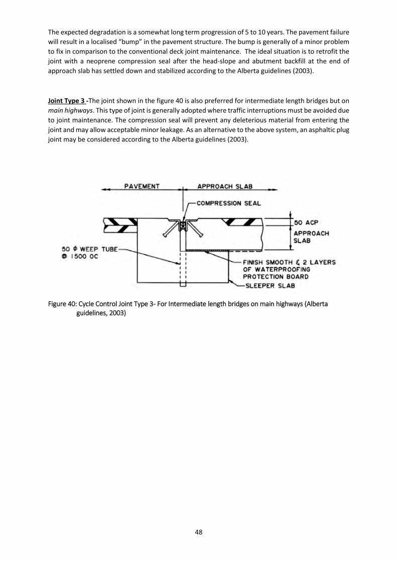
The expected degradation is a somewhat long term progression of 5 to 10 years. The pavement failure
will result in a localised “bump” in the pavement structure. The bump is generally of a minor problem
to fix in comparison to the conventional deck joint maintenance. The ideal situation is to retrofit the
joint with a neoprene compression seal after the head-slope and abutment backfill at the end of
approach slab has settled down and stabilized according to the Alberta guidelines (2003).
Joint Type 3 -The joint shown in the figure 40 is also preferred for intermediate length bridges but on
main highways. This type of joint is generally adopted where traffic interruptions must be avoided due
to joint maintenance. The compression seal will prevent any deleterious material from entering the
joint and may allow acceptable minor leakage. As an alternative to the above system, an asphaltic plug
joint may be considered according to the Alberta guidelines (2003).
Figure 40: Cycle Control Joint Type 3- For Intermediate length bridges on main highways (Alberta guidelines, 2003)
49
Joint Type 4 – This joint as shown in Figure 41 is adopted for long span integral bridges, a large
neoprene strip seal or finger joint may be used. This large joint requires proper support from a piled
grade beam as they cannot tolerate any settlement. A roof slab connects the end of the bridge deck
such that it can span from the girder end to the grade beam. An approach slab is then provided from
the pile grade beam, beyond the roof slab. The above arrangement in Figure 41 may also be
considered for intermediate length bridges with high traffic volumes (Alberta guidelines 2003).
Figure 41: Cycle Control Joint Type 4- For long bridges (Alberta guidelines 2003)
The Alberta Transportation Board’s (2003) guidelines on the design of integral abutments proposes
joint types as summarised in the Table 10 below, provides general guidance for joint types based on
varying integral bridge lengths.
Table 10: General guidance for joint type for various bridge lengths (Alberta guidelines 2003)
Steel girder bridges Concrete girder bridges Joint Type Approx. movement range
< 40 m < 50 m 1 < 16 mm
40 m to 75 m 50 m to 100m 2 or 3 16 < range < 32 mm
> 75 m > 100 m 4 > 32 mm
50
Figure 42 is adapted from the Ministry of Transportation (Ontario) and was developed with the aim to
improve the riding quality and also to reduce frequent repair work. The detail shown in Figure 42 is
for integral bridges where the total length is more than 75m for steel structures and 100m for concrete
bridges. One should note that this is somewhat different to the type 4 expansion joint discussed
previously yet the limitations are the same (Husain & Bagnariol, 2000).
Figure 42: Expansion joint detail at the end of Integral Abutment approach slab (Husain & Bagnariol, 2000)
It could be argued that the integral abutment bridge concept moves the problem of an expansion joint
from the bridge end to the approach slab end. However the North American opinion suggests that it
is more economical and convenient to repair a damaged joint between the approach slab end and the
highway itself rather than to do repairs to the expansion joint on the bridge deck itself. In places where
de-icing salts are used, the leakage of expansion joints results in the spread of detrimental chloride-
laden liquid. The chloride impregnation damage to the concrete elements and bearings (if used) is
certainly more difficult and troublesome than repairing the premix layer at the end of approach slabs.
The actual thermal movements that take place daily are much less than the theoretically calculated
movements and it is the seasonal or extreme variations that lead to the rare limit state conditions
(Lee, 1994). The de-icing salts and daily/ seasonal temperatures discussed by Lee (1994) is not
applicable to most areas in South Africa.
51
It is important that the designer, before adopting an integral bridge design concept, considers all the
constraints. Some additional matters over and above the normal structural evaluation are listed below
by Lee (1994), as:
I. Climatic effects in the area
II. Soil-structure interaction evaluation
III. Traffic intensity, urban or rural
IV. Quality / budget of maintenance authority
V. Consequence of low performance
VI. Accessibility for repairs and the ease of lane closures etc.
During the construction of an integral bridge isolation joint, the quality control and the preparation of
the sub-base greatly influences the long term durability and working functionality of the joint. A well-
constructed expansion joint should be placed on a well compacted sub-base layer between sawn cut
edges. The Figure 43 shown below illustrates an example of a well-constructed joint (Husain &
Bagnariol, 2000).
Figure 43: Integral Bridge joint that is performing adequately (Husain & Bagnariol 2000)
52
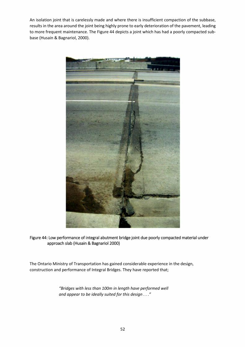
An isolation joint that is carelessly made and where there is insufficient compaction of the subbase,
results in the area around the joint being highly prone to early deterioration of the pavement, leading
to more frequent maintenance. The Figure 44 depicts a joint which has had a poorly compacted sub-
base (Husain & Bagnariol, 2000).
Figure 44: Low performance of integral abutment bridge joint due poorly compacted material under approach slab (Husain & Bagnariol 2000)
The Ontario Ministry of Transportation has gained considerable experience in the design,
construction and performance of Integral Bridges. They have reported that;
“Bridges with less than 100m in length have performed well
and appear to be ideally suited for this design . . .”
53
3.5 Integral Abutment Bridge Transition Slabs
“Bridges of this type are widely spread in the United States but are also becoming popular in
Europe, but the technical solutions are very different in different countries”
Frangi, Collin & Geier - 2011
The previous section discussed different types of isolation joints / expansion joints generally adopted
at the end of integral abutment transition slabs. The transition slabs in the previous section were
directly below the graded premix level. The statement above by Frangi et al (2011) refers to how
various technical solutions are implemented by different organisations or countries. This section
discusses the transition slab of integral abutment bridges, the concept differs from the previous
section.
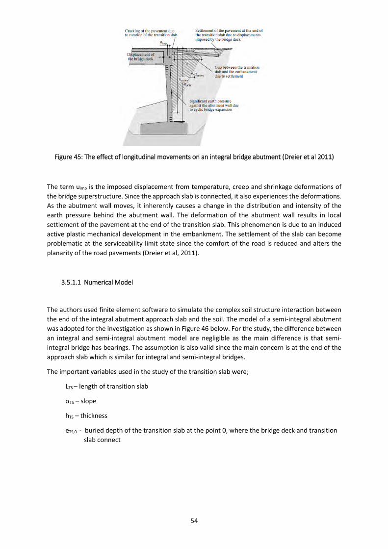
3.5.1 Summary of Research Work by Dreier, Burdet & Muttoni (2011)
One of the main issues with integral abutment bridges is the soil structure interaction, in particular
between the compacted embankment and the transition slab or approach slab. For integral abutment
bridges the transition slabs are directly connected to the end of the integral abutment deck. This
chapter discusses an “alternative” where the transition slab end has no expansion but is rather buried
under the premix layer into the actual layerworks. Dreier et al (2011) discuss the settlement of the
pavement at the end of the transition slab and the cracking that forms in the premix pavement layer
as shown in Figure 45 and thus requires in modifying details of the transition slab.
The use of conventional bridges with expansion joints can lead to costly and complicated maintenance
issues as these mechanical elements must be replaced every 20 to 30 years as discussed in section
2.1.2. These degradations are significant for countries where de-icing salts are used such as
Switzerland; also for bridges exposed to coastal areas and cold temperatures. The problem of de-icing
salts is not relevant to South Africa as snow on the roads is not a major issue compared to countries
such Switzerland. The replacement of bridge expansion joints in South Africa depends on a number of
factors such as the type of joint, the regular maintenance and checking of the existing joint and also
the initial installation of the joint. Joints and /or seals generally need to be replaced between 10 to 15
years in South Africa.
54
Figure 45: The effect of longitudinal movements on an integral bridge abutment (Dreier et al 2011)
The term uimp is the imposed displacement from temperature, creep and shrinkage deformations of
the bridge superstructure. Since the approach slab is connected, it also experiences the deformations.
As the abutment wall moves, it inherently causes a change in the distribution and intensity of the
earth pressure behind the abutment wall. The deformation of the abutment wall results in local
settlement of the pavement at the end of the transition slab. This phenomenon is due to an induced
active plastic mechanical development in the embankment. The settlement of the slab can become
problematic at the serviceability limit state since the comfort of the road is reduced and alters the
planarity of the road pavements (Dreier et al, 2011).
3.5.1.1 Numerical Model
The authors used finite element software to simulate the complex soil structure interaction between
the end of the integral abutment approach slab and the soil. The model of a semi-integral abutment
was adopted for the investigation as shown in Figure 46 below. For the study, the difference between
an integral and semi-integral abutment model are negligible as the main difference is that semi-
integral bridge has bearings. The assumption is also valid since the main concern is at the end of the
approach slab which is similar for integral and semi-integral bridges.
The important variables used in the study of the transition slab were;
LTS – length of transition slab
αTS – slope
hTS – thickness
eTS,0 - buried depth of the transition slab at the point 0, where the bridge deck and transition
slab connect
55
Figure 46: (a) Geometrical model adopted for the numerical analysis; (b) definition of slope variation
criterion c (Dreier et al, 2011)
According to Figure 46a, the assumed geometry of the transition slab is consistent with the Swiss
recommendations for transition slabs of integral abutment bridges.
LTS – length = 6m
αTS – slope = 10%
hTS – thickness = 0.3m
eTS,0 - buried depth of the transition slab at the point 0, were the bridge deck and transition
slab connect = 0.1m
The thickness of the premix in the model was 70mm. The slope of the road αroad is assumed to be zero
and this variable does not influence the results. The imposed displacement (uimp) for the study was
chosen to equal 50mm.
The Swiss recommendations discussed above is generally similar to the approach slabs constructed in
South Africa.
3.5.1.2 Road Pavement Planarity Limit State
A slope variation criterion c according to the Swiss code was adopted to quantify the planarity of
the road. It considers the depth and length of the settlement and yields an efficient evaluation of the
local curvature, thus the comfort of the road. This slope variation c must always be less than the
limit value of cadm (admissible slope variation) and according to the Swiss codes cadm is equal to 28%
for normal roads and 20% for highways.
To investigate if the imposed displacement is uimp is acceptable for road users i.e. it must pass limiting
value of cadm. The Figure 47 was generated by plotting the maximum and minimum values of c in
56
the range of the transition slab displacement. The useful parameter from this graph is obtaining the
maximum admissible displacement uimp,adm for a given cadm.
Figure 47: Graph showing admissible imposed displacement (uimp,adm) for cadm of 20% based on the
Swiss codes (Dreier et al, 2011)
The admissible imposed displacement uimp,adm for highways (c=20%) for the standard geometry of a
transition slab provides 43mm. According to the Swiss national codes if a total imposed deformation
eimp = - 0.8mm/m for a concrete bridge deck (sum of ecr= - 0.2, ec,sh= - 0.35mm/m and
eDT = -0.25mm/m due to DT= - 25 Co), this provides a maximum distance between the concerned
abutment and the fixed point of the bridge deck of 54m.
Bridge ends that undergo major retrofitting to transform a conventional bridge into a bridge with
integral or semi-integral abutments do not have to consider creep and shrinkage effects. It is assumed
that the creep and shrinkage effects on a conventional bridge have already taken place. Thus for
admissible imposed displacement uimp,adm of 43mm and assuming a residual deformation of
eimp = - 0.4mm/m, the maximum possible length between the newly converted integral abutment and
fixed point of the bridge is 108m. Thus, the longest possible length of a bridge with two retrofitted
abutments and fixed point in the centre is 216m.
The situation that generally governs is for movement away from the abutment i.e. active soil
conditions. Research has shown that in the passive direction, the settlements in this case are
significantly less problematic because the displacement to activate the passive plastic mechanism is
much higher than for active mechanism conditions. For concrete conditions the active mechanism also
has creep and shrinkage in the active direction.
3.5.1.3 Cracking of the Road Pavement at the Bridge Deck and Transition Slab Interface
The displacement of the transition slab can lead to cracking of the road pavement at the connection
between the transition slab and the bridge deck as shown in the Figure 48 below. These cracks
57
generally occur during the winter season when the road premix is brittle due to low temperatures.
The low temperatures (i.e. below 0o) is very localised, and occurs only in certain regions of South
Africa. The cracks are a result of the following:
Rotation of the transition slab around the connection due to settlement behind the
abutment wall induced by the imposed displacement.
Repeated deflections caused by flexure when trucks and heavy vehicles move over the
transition slab.
Figure 48: Cracking of the road pavement at the transition slab and bridge deck interface for a 68m semi-integral bridge (Dreier et al, 2011)
3.5.1.4 Improved Connection Detail of the Transition Slab and Integral Abutment
Figure 49, below shows a connection detail with a dowel bar where the transition slab rotates around
the steel stud. The rotation propagates to the surface thus this detail is prone to localised cracking.
This detail is unfortunately not ideal for integral or semi-integral bridges because the stud/dowel
connection is too weak to transfer the longitudinal forces generated from the displacements.
Figure 49: Standard abutment/transition slab joint with dowel bar (Dreier et al 2011)
Figure 50, below shows the detail currently recommended in Switzerland for integral abutment decks.
This detail is favourable with respect to cracking as the centre of rotation of the transition slab is at
the level of the connection reinforcement. This connection can carry the internal forces from imposed
58
displacements. This detail is slightly difficult to construct as it is monolithic with the abutment and the
bitumen layer (no.11 as shown in Figure 50) must be placed before the connection reinforcement is
fixed.
Figure 50: Detail of abutment/transition slab for integral abutment bridges according to Swiss recommendations (Dreier et al 2011)
Figure 51, below is an improved detail by Dreier et al (2011) and adopts the principle of a concrete
hinge. The reinforcement is such that the shear failure is prevented by diagonal connection
reinforcement. The construction is simpler and the distribution of the rotation of the transition slab
over the entire length of the concrete hinge lch. The cracks from this detail showed small openings that
cannot propagate to the road surfacing.
Figure 51: Improved detail for integral abutment bridges (Dreier et al 2011)
59
3.6 Behaviour of Piles Supporting Integral Abutment Bridges
SUMMARY OF RESEARCH WORK BY ARSOY, DUNCAN AND BARKER (2002)
The literature regarding the behaviour of piles supporting integral abutment bridges under cyclic
loading is limited. Published papers on this subject used actual behaviour of the following bridges;
Cass County Bridge
Boone River Bridge
Maple River Bridge
And a bridge in Rochester, Minnesota.
These bridges were monitored for approximately 2 years. They were subjected to real-life
temperature cyclic loading. A summary of the bridge details and behavioural performance is discussed
in Table 11.
Table 11: Summary of Integral Bridge pile details and performance (Arsoy et al 2002)
Bridge Name
Location Overall Length (m)
Type of superstructure
Type of Piles & Orientation Pile Behaviour and results from monitoring period (mm)
Cass County Bridge
North of Fargo – North Dakota
137 m (6 Spans)
Concrete deck & Prestressed concrete girders
HP 10x42 Piles orientated in weak-axis bending under abutments and strong-axis bending under piers.
6.1m predrilled boreholes were used.
During monitoring period, strain gauges failed. Stress was based on analytical methods and concluded that maximum pile stresses were around yield stress.
Piles were able to tolerate 50mm bridge contraction and about 75mm total displacement.
Boone River Bridge
Central Iowa
98.9m (4 spans) & skew of 45 degrees
Concrete deck & Prestressed concrete girders
HP 10x42 Piles orientated in weak-axis bending and battered 4:1 in the movement direction of the bridge.
2.74m predrilled boreholes were used.
Maximum pile stress was about 60% of nominal yield stress of piles
Bridge experienced 30mm contraction and about 50mm total displacement without any damage to piles.
Maple River Bridge
Northwest Iowa
97.5m (3 spans) & skew of 30 degrees
Composite Concrete deck & steel girders.
HP 10x42 Piles orientated in weak-axis bending and battered 3:1 in the movement direction of the bridge.
3.66m predrilled boreholes were used.
Maximum pile stress was about 75% of nominal yield stress of piles
Bridge experienced maximum 40mm contraction and total bridge displacement was around 76mm.
Bridge in Rochester
Minnesota 66m (3 spans)
Concrete deck & Prestressed concrete girders
Integral abutments are 0.9m wide and 1.5m high.
Supported on HP 12x53 piles orientated in weak-axis bending.
Piles were able to tolerate 20mm bridge contraction and 32mm total displacement
Maximum pile stresses slightly above nominal yield stress of piles
Laboratory testing was performed on different types of piles by simulating them to similar conditions
as piles supporting integral abutment bridges and conclusions regarding their performance have been
reported. The piles were subjected to 75 years of simulated bridge life by subjecting the piles to cyclic
lateral load tests. Over 27,000 displacement cycles were applied. The piles investigated were an H-
pile, a pipe pile and a prestressed reinforced concrete pile.
60
“Bridge superstructures are so stiff in comparison with approach fills and piles
supporting abutments that the magnitude of the temperature-induced displacements
are almost unaffected by the stiffness of the abutment piles. The stiffest abutment piles
and the most flexible abutment piles are subjected to the same displacements. The
ability of the piles to accommodate lateral displacements without distress is a
significant factor in determining the maximum possible length of integral bridges,
because temperature-induced displacements are proportional to bridge length.”
(Arsoy et al 2002)
The statement above by Arsoy et al (2002) argues that due to the high difference in stiffness between
the superstructure and abutment piles, any thermal movements will cause the pile to deform
accordingly irrespective of the pile stiffness. This is also an important key for determining the
maximum possible lengths of integral bridges. The piles behave as an equivalent cantilever with a free
head at the top of pile easily moving to accommodate the deck thermal movements. The concept is
illustrated in the Figure 52 i.e. pile is fixed at one end and free headed at the other end.
Figure 52 shows the configuration that was used in the laboratory testing. For convenience the test
pile cap and pile were inverted. It is important to note that the study does not include soil-structure
interactions. The investigation studies the pile behaviour under realistic cyclic displacements induced
due to thermal effects.
Figure 52: Pile and pile cap configuration adopted for laboratory testing (Arsoy et al 2002)
The three types and details of the piles used for the testing are listed below;
The H-pile that was tested was an HP 10x42.
The pipe pile had a 356mm outer diameter and 12.7mm wall thickness.
The prestressed concrete pile that was adopted was a square pile (305mm x 305mm). Five
12,7mm, 1862 MPa low relaxation steel strands were used in the pile.
Table 12 provides more details of the piles used in the investigation.
61
Table 12: Properties of piles tested in the laboratory investigation (Arsoy et al 2002)
The Figure 53 shown below is a schematic diagram showing the fixity of the pile cap at one end.
Figure 53(a) is the plan view and Figure 53(b) is the cross-sectional view.
Figure 53: Method adopted for mounting pile caps for the laboratory investigation (Arsoy et al, 2002)
62
The Figure 54 is a photograph of the test that was conducted in the laboratory.
Figure 54: Photograph of experimental setup (Arsoy et al 2002)
Results and recommendations from investigation by Arsoy et al (2002)
H-pile Test
The investigation showed that for a given load, the maximum measured strain was about half of the
strain calculated for a fixed-end column (pile was free at one end and fixed at the other end). The
reason for this behaviour was because the pile cap was not fully fixed against rotation. Pile
displacements were plotted along the pile for selected loads as shown in Figure 55. The graph shows
that the slope at the bottom of the pile is not zero, which indicates there is some rotation of the pile
cap thus the pile behaves as a “partially fixed column”. The H-pile, when orientated about its weak
axis displayed the best behaviour of the piles tested. The pile experienced cyclic loading stress in
excess of 138 MPa and static loading stress of 241 MPa without any signs of distress and deformation.
“This superior level of performance under cyclic loading makes H-piles a good choice for
support of integral bridges.
(Arsoy et al 2002)
63
Figure 55: Graph showing displacements for H-pile based on selected lateral loads (Arsoy et al 2002)
Pipe Pile Test
The pipe pile was approximately twice as stiff as the pile cap thus the pile cap of the pipe pile rotated
more than that of the H-pile. No damage was observed on this type of pile. The researchers anticipated
that an abutment supported by this type of stiff pile would be subjected to higher stresses because
the loads required to deflect the pile would be larger. The piles could support an integral abutment
bridge but special attention should be given to the design details to prevent damage due to cyclic
loading as advised by the authors.
Prestressed Concrete Pile Test
In the first trial, tension cracks developed at the bottom of the pile where it was connected to the pile
cap. During the testing the tension cracks gradually increased in the pile from the bottom and
progressed to the top. It was also noted that the five cracks gradually enlarged as the load cycles
continued. Figure 56 shows a typical tension crack through one of the strain gauges. The concrete piles
were tested with no vertical load and it was anticipated that more severe damage to the piles would
have occurred with vertical loads. At the end of the test, it was observed that approximately 20% of
the original pile cross-sectional area was still in contact. The vertical load would have induced a very
high compressive stress due to the significantly reduced cross-sectional area. The research concluded
that the use of concrete piles to support integral abutment bridges is not the best solution due to the
formation of cracks with a gradual increase of cracks under cyclic loading, and more research work
was required.
64
Figure 56: Formation of tension cracks on the precast concrete pile (Arsoy et al 2002)
65
3.7 Pile Pre-Drilling and Sleeving of Piles
Piled abutments are commonly used in North America for integral abutment bridges. As discussed in
the previous section, the research by Arsoy et al (2002) found that, for integral abutment piles, it is
advantageous that the piles can accommodate any lateral displacements induced from the deck.
Designers have thus adopted techniques such as (Card & Carder):
I. Adopting slender piles such as steel H-piles or precast concrete piles
II. To improve the flexing behaviour, limit the number of piles to a single row
III. Orientate piles vertically to minimise resistance
IV. Orientate the weak axis of H-piles normal to the direction of movement
V. Where the insitu foundation materials are very stiff or rigid, oversized pre-bored holes are
used. The primary purpose of pre-boring is to allow the upper zone of the pile to have
sufficient flexibility to deflect without the rigid soil restraining the movement. The pre-bored
holes are typically 2m to 5m deep. Prior to the installation of the piles they are filled with
loose granular material (Girton 1991 cited in Card and Carder 1993)
VI. Piles are generally limited to steel H-piles as they have longer fatigue life
VII. Reduce depth of abutment embedment into embankments to reduce resistance
VIII. Control bridge skews
An alternative to pre-boring as discussed by the guidelines for design of integral abutments by Alberta
Infrastructure and Transportation (2007) is to install the single row of steel H-piles in permanent steel
casings, also orientated for weak-axis bending. However due to the probability of the loose granular
fill being compacted over time thus restraining the pile, it is preferred to leave the casing voided unless
some type of elastic fill material is adopted.
Some other relevant considerations that the guideline provides are listed below;
I. Steel casing around piles should be designed to last the same life span of the bridge
II. A sacrificial corrosion thickness should be allowed for in the pile section
III. The H-piles should be embedded at least two pile sizes into the abutment beam
66
The Figure 57 shows a schematic diagram of a steel H-pile that is isolated by using a corrugated steel
pipe (CSP) and filled with loose sand.
Figure 57: Integral abutment bridge piles with sleeve detail as per Ontario Ministry of Transportation (Husain & Bagnariol, 1996)
67
The Figure 58 shown below is a photograph of a single row of steel H-piles being isolated by using
pipes around the pile.
Figure 58: Corrugated plastic pipe sleeving around steel H-piles used in UK (White 2007)
A European Survey conducted revealed that some countries such as England and Sweden adopt
sleeves around the piles to easily allow for the free bending of the piles due to superstructure
translations. The longitudinal translation is distributed along a greater length of the freestanding pile
thus the moment induced in the pile is reduced. Since there is no soil around the pile shaft to prevent
buckling, the pile inherently behaves similar to a freestanding column thus requires durable piles to
accommodate the unsupported length. One of the disadvantages is that once backfill is around the
sleeves, inspections of piles is virtually impossible (White 2007).
68
3.8 Front Elevation of Integral Bridge Abutments
The front elevation of integral abutment bridges predominantly depends on what the bridge primarily
spans over and the purpose for the bridge. Most integral bridge abutments generally act as a typical
pier to simply achieve sufficient flexibility whilst the soil mass behind the abutment is retained by
separate retaining mechanisms. A commonly adopted mechanism used with integral abutments is the
use of mechanically stabilised earth retaining walls. Figure 59 shows the different concepts for integral
abutments generally constructed (Concrete Bridge Development Group 2014).
Figure 59: Different concepts for Integral abutment bridges (Concrete Bridge Development Group, 2014)
69
Figure 60 shown below is the front elevation of an integral bridge abutment with the fill being retained
by mechanically stabilised earth retaining walls. The superstructure consists of prestressed beams
with a top slab.
Figure 60: Integral abutment with retained soil system (Ontario Ministry of Transportation 2008)
Figure 61 is a cross-section of an integral abutment bridge showing the soil retaining system and the
isolation of the piles in the top few meters.
Figure 61: Section of integral abutment showing sleeves around piles and retained soil system in place (Ontario Ministry of Transportation 2008)
70
3.9 Nature of Backfill behind Integral Abutment Bridges
The backfill material behind integral abutments should be a designed material with specified
properties that are validated during the construction phase. The specification should cover two
important aspects; stiffness and flexibility. Well-rounded compacted granular material of uniform
grading can provide a peak angle of internal friction (F) of about 35°. This may accommodate the
thermal expansion without inducing high earth pressures but may undergo settlement. On the other
hand, well graded and compacted, hard angular particles may produce a peak angle of internal friction
as high as 55°. This will have very high resistance to thermal movements and less vulnerability to
settlement. According to the BA 42/96 Highways Agency guidelines (2003), for integral bridges
exceeding 40m, the granular backfill should have a peak angle of friction of not greater than 45° when
tested in accordance with the Specification for Highway Works. The zone of granular backfill should
be an angle of at least 45° from the bottom of the wall extending to the top (BA 42/96 Highways
Agency guidelines 2003).
3.10 Chapter Summary
Based on the calculated movement of the superstructure the bridge designer should appropriately
select the expansion joint as proposed in Section 3.4 of the literature review. The most suitable type
of expansion joint to be chosen for the end of the approach slab is suggested in Table 10, adapted
from the Alberta Guidelines (2003) which are widely used. The designer also has the option of not
using any expansion joint at the end of the approach slab. This concept is discussed by the research
done by Dreier, Burdett and Muttoni (2011). This concept has no form of joints as the approach slab
is embedded within the road layerworks fill, however it is anticipated that a “bump” in the roadway
may result. This issue of the undulation in the road surface is not considered a major serviceability
concern provided it is within tolerable limits as proposed by Dreier et al (2011). The second concept
of no joint is assumed to be most appropriate, however the integral bridge length is limited to a
maximum of 108m as discussed in the research work.
Integral bridges have numerous advantages but also has their own unique challenges. The main aim
of this chapter was an extension of Chapter 2 addressing issues and solutions proposed concerning
integral bridge abutments. This chapter introduced the soil-structure interaction and discussed a few
design concepts such the equivalent cantilever method. The equivalent cantilever method is widely
used by many bridge design offices to design the piles for integral abutment bridges. The
fundamentals of laterally loaded piles were briefly described. Other solutions to isolate the soil and
structure were introduced such as adopting a stress-absorbing layer behind the abutment structure.
An important aspect regarding the ratcheting effect and failure was discussed and concepts using
stress-absorbing layers where introduced. Under the latter subject, the approach slab and sleeving of
piles was introduced and is an important practice to try and increase flexibility of the abutment
system. The approach slab for integral abutments is slightly different to convention bridge abutments.
The concepts presented showed that the approach slabs are generally fixed for integral bridge
abutments and not pinned as per the conventional. This chapter also presented interesting findings
on the behaviour of different pile types under cyclic loading. As per the literature from various authors,
the investigation showed that the steel H-pile is very superior for this type of application. There are a
number of issues and challenges with integral abutment bridges, however there are just as many
concepts and theories at present to resolve these problems.
71
CHAPTER 4
4 PROCEDURE OF INVESTIGATION
4.1 Introduction
The aim of the investigation was to identify some of the suitable pile types that a bridge designer
should consider for an integral abutment bridge and to understand their behavioural performance.
Various pile types that are commonly used for conventional bridges in South Africa were adopted in
the study such as PC piles and auger piles. Steel H-piles and pipe piles are not common in South Africa
but were considered in the investigation for comparative purposes as they are usually adopted in
integral bridges in other countries, as shown by the research in Section 2.4 from the literature review.
Other piles are also used for integral bridges but there are certain concerns as highlighted in Section
3.6, the research work done by Arsoy et al (2002).
The theoretical desktop study simplifies the analysis of piles by disregarding the soil spring interaction
which was discussed in section 3.1.2.1, thus considering the pile to act as an equivalent cantilever
column. Some authorities design integral abutment piles by modelling in the soil spring stiffness while
many other bridge authorities have mastered the equivalent cantilever pile concept method. Many
integral abutment bridges have been designed successfully by adopting the equivalent cantilever pile
concept such as the M50 Freeway Bridge in Ireland (Figure 18). Ontario also adopts pile design using
the equivalent cantilever method and the results are reported as being reasonable. Another reason
this method is favourable is because the top portion of piles for integral abutment bridges is generally
free as it is sleeved to allow sufficient flexibility to accommodate the deck movements as discussed in
Section 3.7 and examples provided in Table 11. The bottom of pile is almost fixed into the ground, free
along the sleeve and able to accommodate the deck movements at the top of pile, thus the idealisation
as a cantilever is reasonable.
The approach taken in this investigation aims to provide the designer with a rudimentary
understanding of the behavioural performance of the pile type that should be adopted. To obtain
more accurate results, the designer should perform further analysis with soil spring stiffness and
appropriate software, if required. The spring constants often remain a challenge and some guidance
is provide in Section 3.1 and 3.2.
4.2 Formulas and Methods Adopted
Different types of piles were chosen for the study to determine the behaviour of piles for integral
abutment bridges. The length of the effective cantilever of the pile was also varied and a number of
cantilever lengths were used in the study to investigate the relevant parameters. The guidance for
choosing suitable effective cantilever lengths was discussed in Section 3.7 and typical examples
provided in Table 11. The lengths used (also referred to as effective pile height) were 2m, 3m, 3.5m
and 4m.
72
It is important to note that the study was based on the pile being fixed at the bottom and free at the
top i.e. free pile head. This assumption is supported by the work done by Arsoy et al (2002) as
discussed in Section 3.6. The statement at the top of page 60 describes how irrespective of the
stiffness of the piles, the superstructure is considerably more stiffer and any displacements from the
superstructure (e.g. thermal movements) will directly result in the piles absorbing and moving
accordingly to the magnitude of this movement. The work done by Arsoy et al (2002) implies that the
top of pile is essentially free to move although it is fixed to the deck. This theory is backed up by Figure
52 which shows the actual orientation on a construction site, and the equivalent system in the
laboratory. The model also shows no springs as in most cases the top zone of the pile is within a sleeve.
The discussion above assumes that the soil behind the abutment is not involved in restraining the
movements from the deck. As highlighted in Chapter 3.3, common practice in many countries is to
isolate the structure from the soil thus preventing the ratcheting effect discussed in Section 3.3.2. This
is often done by adopting a mechanically stabilised earth retaining wall to hold the fill material and
using a stress-absorbing layer (e.g. expanded polystyrene) directly behind the abutment as
emphasised in Section 3.3.3 and illustrated in Figure 30. Coupled with this detail is a joint used at the
end of the approach slab as discussed in Section 3.4.
There are two scenarios to consider regarding the deflection of vertical piles carrying lateral loads as
discussed by Tomlinson (1994);
I. Free pile head – top of pile is unrestrained and tends to rotate and undergo a degree of
. translation.
II. Fixed pile head – top of pile is restrained (fixed) to the pile cap or braced but has the
. freedom to translate.
Figures 62 and 63 shown below illustrate this concept. Based on the findings in the literature review
the free headed pile was adopted, but fixed headed pile is shown for comparative purposes.
Figure 62: The cantilever concept of free pile head and fixed pile head (Tomlinson 2004)
73
Figure 63: Bending of pile under vertical and horizontal loads (a) Partially embedded pile; (b) Equivalent cantilever pile (Tomlinson 2004)
The analysis made use of the following equations which were derived from structural theory as the
piles under horizontal load are considered as simple cantilevers (Tomlinson 2004). The derivations are
shown in Appendix F.
1) Horizontal deflection at head of fixed-headed pile: 𝑦 = 𝐻(𝑒+ 𝑧𝑓)3
12𝐸𝐼
2) Horizontal deflection at head of free-headed pile: 𝑦 = 𝐻(𝑒+ 𝑧𝑓)3
3𝐸𝐼
Where:
y = Horizontal deflection at the head of pile investigated about each axis
H = Horizontal force at the head of pile
E = Elastic modulus of material forming the pile shaft
I = Moment of inertia of the cross-section of the pile shaft
zf = Assumed arbitrary depth to point of virtual fixity
e = Free length of pile shaft
The analysis was done by calculating the typical range of movements of integral abutment bridge
decks (according to the formula discussed above). The same amount of translation was assumed to
be transferred to the top of pile heads. The effective pile height refers to the length of the pile that is
sleeved i.e. Length of pile sleeve = zf + e.
74
The important results obtained from this study were pile bending moments and pile shear forces. The
most important aspect that these parameters are associated with is the translation or deflection at
the head of the pile as these are the typical translations of the actual bridge deck at the abutments
due to thermal effects, creep and shrinkage as discussed in Sections 2.3.1 and 2.3.2 respectively. The
relationship between slenderness ratios and stiffness of the piles was also investigated.
Table 13 shown below contains details of the piles chosen for this study. The concept was adapted
from the work done by Arsoy et al (2002) discussed in the literature review. The study done by Arsoy
made use of steel H-piles (both axes investigated), a pipe pile and a square precast concrete pile. The
authors recommended that more research on the different types of pile for integral abutment bridges
should be carried out.
Table 13 lists the typical piles used in South Africa such as the square precast pile and the 600mm
diameter auger pile. The H-pile is not generally used in South Africa due to the high costs (Section
2.4.1.1) but had to be investigated to check if other more common feasible piles can be substituted
for steel H-piles. Pipe piles are also not commonly used in South Africa but were considered to
understand the behaviour of a stiff pile. The material strengths shown in Table 13 are commonly used
Moments for Different Pile Types - 3,5m Effective Height (free head)
350 x 350 250 x 250 H-P (SA) H-P (WA) Pipe Pile Pile Deflection (Example)
89
Figure 81 shown above indicate the order of the stiffness of the piles i.e. (as listed in decreasing
stiffness based on the linear curve);
1. 600mm diameter concrete pile (not shown in graph above but in Appendix C)
2. 350 x 350 PC concrete pile
3. Steel Pipe pile
4. H-pile, bending about strong axis
5. H-pile, bending about weak axis
6. 250 x 250 PC concrete pile
One should note that the H-pile along its weak axis and the 250 x 250 PC pile are very comparable in
terms of flexibility, moments and shear. From this behavioural characteristic this could imply that if
steel H-piles in South Africa are expensive to manufacture, the 250 x 250 PC pile could be used as an
alternative. For approximate cost comparison, consider a 350 x 350 PC pile to be supplied and installed
would cost about R 850.00/m, a 600mm diameter auger pile about R790.00/m whilst a steel H-pile to
be supplied and installed would cost in the range of R 1500.00/m to R 3000.00/m (all establishment
and de-establishment cost have been ignored). From Figure 81, although the 250 x 250 PC and H-pile
(weak axis bending) are comparable, the deflection limit on the 250 x 250 PC pile is much smaller than
that of the H-pile.
It is also important to acknowledge the results from Arsoy et al (2002), where the research concluded
that PC concrete piles when subjected to cyclic loading are prone to forming tension cracks. The most
appropriate pile based on the Figure 81 above and considering the work done by Arsoy et al (2002) is
thus an H-pile positioned along its weak axis. The graphs above explain why the extensive literature
of integral abutment bridges strongly recommend the steel H-pile to be adopted along its weak axis.
This certainly does not imply that other piles are not applicable. In Germany for example, concrete
foundation piles and sub-structure are used for integral bridges but to attain the required flexibility
different types of aggregate are carefully blended to essentially reduce its stiffness (Young’s Modulus).
If the PC piles are prone to tension cracking, perhaps additional reinforcement and /or pre-tension
wires need to be included to make them more ductile. The final decision is based on which pile the
designer chooses and which pile passes all the checks, requirements, costs and availability.
90
Table 14 shown below is the pile results for the example illustrated in Chapter 4. Table 14 below shows
a summary of moments of the pile at the point of virtual fixity (bottom of the pile). The designer should
check if the proposed pile section can accommodate these inherent parameters as well as all other
additional loading as per TMH7 (parts 1 and 2) as discussed in Section 2.2 of the literature review. The
number of piles adopted is very important as the forces applied must be within the working load of
the pile and the reinforcement (or prestress) should be able to accommodate for such vertical loads.
One should note that since the pile now behaves as a column within the sleeve, the pile section has
the probability of actually having a working load less than what the pile manufacturer or piling
guidelines propose, thus performing this check is important. Second order effects should also be
considered. The cost factor plays an important role but the long term performance of the pile must
also be thoroughly investigated. Calculations for the example scenario are provided in Appendix C and
Appendix E).
Table 14: Summary of results obtained from the 3,5m effective cantilever pile length data for varying pile types (values are all un-factored i.e. at SLS)
Proposed Piles 3.5m effective cantilever graph
(free-headed pile)
Pile Type Pile Details Movement
of deck due
to temp,
creep &
shrinkage
(mm)
Moment at
point of fixity
(kNm) –
From Figure 81
Stress
Calculation
(N/mm2)
(Appendix E)
Square Precast
Concrete pile
350 x 350 13 112
N/A (limit
exceeded)
Square Precast
Concrete pile
250 x 250 13
29 11.14
Circular
Augered Pile
600 Diameter 13
- -
H-Pile (strong
axis)
254 x 254 x 89 13
94 83.48
H-Pile (weak
axis)
254 x 254 x 89 13
31 81.51
Pipe Pile 356 Outer
Diameter
(10mm wall
thickness)
13
104 113.71
The required movement in the example scenario was calculated to be 13mm thus according to Table
10 from the literature review, a Type 1 joint would suffice at the end of the approach slab. The
alternative of embedding the approach slab in the layer works material is also appropriate, however
special connection details must be adopted as discussed in Section 3.5.
91
CHAPTER 6
6 CONCLUSIONS AND RECOMMENDATIONS
6.1 Conclusions
Integral abutment bridges of the form and concept discussed in this dissertation are relatively new to
South Africa. Many countries have strongly favoured this type of bridge especially when bridge lengths
are within a small to medium range. There are numerous benefits associated with integral abutment
bridges by just considering the maintenance aspects, but a poor design or lack of understanding of the
concept could prove to be problematic for the bridge authority as it will require regular maintenance
thus leading to high unanticipated costs.
One of the most challenging issues with integral abutment bridges is the soil-structure interaction.
The concept of modelling the soil as a spring is often used but modelling the piles as an equivalent
cantilever is also very widespread and popular. This research demonstrates that it is possible as the
reasoning behind adopting the equivalent cantilever method is appropriate when pile sleeves or
similar are used. The tops of piles should be given allowance to be free and flexible to accommodate
any movements from the deck. The abutment back face should be lined with an appropriate geofoam
and of the correct thickness to avoid compression set when loads are released. The approach slab for
integral abutment bridges is very important and the details of integral abutment bridge transition
slabs are different when compared to conventional bridges.
The research work shows that if the pile is flexible and/or the appropriate equivalent pile cantilever
length (i.e. free pile within a sleeve) is adopted then the corresponding bending moments and shear
force at the point of virtual fixity are minimal. A steel H-pile positioned along its weak axis proves to
be superior compared to other types of pile, also considering the ductility and durability for the long
term cyclic movements the pile needs to accommodate. The influence of pile sleeves or pre-boring is
significant and this research work has shown that the minimum sleeve length should be 3m. Steel H-
piles in South Africa are not commonly used. One of the reasons for this is the high associated costs.
This needs to be carefully weighed-off against costly and maintenance-prone bearings, expansion
joints and with other pile types. Alternative piles types are possible but the designer must be aware
of the limitations such as tension cracks on concrete piles under cyclic loading. Certainly more research
is required on alternative pile types and their behaviour in integral abutment bridges.
Integral bridges have proven to be superior in certain countries as many authorities have mastered
the design of these structures. If these structures are to be adopted in South Africa, and certainly they
should, the first few should be instrumented and behaviours studied in detail and also the
performance analysed after a few years. Caution should be exercised as constructing too many in
haste could result in poor performance only at a much later time due to soil ratcheting effects which
may not be seen in the first few years. One of the most important aspects of integral abutment bridges
is the length. Many countries and authorities have different limiting lengths which are based on their
experience. Similarly, if these type of bridges are used in South Africa they should only be considered
for small to medium spans (overall bridge length of about 60m) and after monitoring the performance,
then only longer lengths should be constructed or allowed. The research work from the literature
92
review concludes that even integral bridges may require some sort of a joint at the end of the
approach slab. One may now argue, that by having the joint, it is essentially moving the problem from
the deck to the end of the approach slab and once again similar to the conventional bridge type where
maintenance is required. If the length is limited then specially detailed approach slabs can be buried
in the roadwork’s fill material and no joint is required as discussed in the literature review.
Integral bridges are not common in South Africa and this is perhaps due to the uncertainty of the soil-
structure interaction, thus bridge designers often choose to adopt bearings and expansion joints.
Overseas the norm is that, if the bridge length is considerably small (< 60m), it is considered standard
practice to adopt an integral bridge arrangement whereas in South Africa it is common to find bearings
and expansion joints on considerably short spans (< 20m). Integral bridge concepts for shorter lengths
need to be adopted in South Africa to reduce the maintenance and replacement costs of bearings and
expansion joints. The issue of de-icing salts is not applicable in South Africa but the issue of bearings
corroding and seizing is not uncommon. The thermal effects in South Africa are somewhat similar to
those covered in the references, as the literature for integral bridges constructed in various countries
with varying temperature ranges indicates that these structures seem to be performing well. The
biggest difference is the piling system specified with the use of steel H-piles not common in South
Africa. However this is certainly possible and does not pose major construction challenges.
The conventional approach in South Africa is that the majority of bridges are designed such that the
bridge abutment (open or closed) are very rigid or stable, with the superstructure seated on bearings
which in turn rests on the rigid abutments. However with integral bridge abutments, the aim is to
design the abutment such that they have a certain degree of flexibility. Perhaps moving away from
the conventional approach may create uncertainties for the bridge designer, initially resulting in some
resistance to the use of integral bridges, however this is easily overcome. Integral bridges are certainly
applicable in South Africa and bridge designers should consider them as appropriate for short to
medium span structures, providing a feasible technical solution as well as reducing maintenance costs.
93
6.2 Future Work
The piles investigated in the desktop study need to be investigated in the laboratory by
simulating an equivalent model. This will establish the actual moments and shear forces
experienced and provide information regarding these values between the fully fixed and fully
free conditions. From this same experiment, it is possible to confirm the work done by Arsoy
et al (2002) and check how the different piles behave under cyclic loading. In South Africa steel
piles are not often used and if precast piles could be adopted then this type of bridge will
certainly become more popular. The research should also include pretension precast piles.
If these bridges of the concept described in this dissertation are to be adopted in South Africa,
the first few should be well instrumented to determine their actual performance.
The concept of the geofoam and elastic material behind the abutment to reduce high passive
pressures will also be better understood if they are somewhat instrumented and performance
monitored while they are actually being used.
Pile sections should also be investigated, that is, designing the top few meters (say 6m) of a
pile of a different section (stiffness) to the rest of the shaft to ensure that pile deflections are
as per the optimal requirements or to accommodate the most appropriate joint.
Option of semi-integral bridges and applicability.
94
REFERENCES
Abendroth, R. E., Greimann, L. F. & LaViolette, M. D., 2007. An integral abutment bridge with precast concrete piles. Report No. IHRB (Iowa Highway Research Board Project TR-438.
Alberta Transportation Board Bridge structure design criteria (2003). Appendix C – guidelines for integral bridge abutments.
Arsoy, S., Barker, R.M. & Duncan, J.M., 1999. The behaviour of integral abutment bridges. Report No. FHWA/VTRC 00-CR3, Virginia Transportation Research Council.
Arsoy, S., Duncan, J.M. & Barker, R.M., 2002. Performance of piles supporting integral bridges. Transportation Research Record: Journal of the Transportation Research Board, (1808), 162-167.
BA 42/06 Highways Agency, 2003. The Design of Integral Bridges. Design Manual for Roads and Bridges. The Stationery Office, London, Vol. 1.2.12.
Benaim, R., 2008. The design of prestressed concrete bridges, concepts and principles. Abingdon, UK: Taylor & Francis.
Bezgin, O., 2010. An insight into the theoretical background of: Soil structure interaction analysis of deep foundation. Lecture notes/website, Istanbul, January 2010.
Bowles, J. E., (1996). Foundation analysis and design. 5th ed. New York: McGraw-Hill Companies
Broms, B. B., 1965. Design of laterally loaded piles. Journal of Soil Mechanics & Foundations Division, Proceedings of the American Society of Civil Engineers, Volume 91, p 79-99.
Burke Jr, M. P., 2009. Integral and semi-integral bridges. United Kingdom: John Wiley & Sons.
Byrne, G., Everett, J.P. & Schwartz, K., 1995. A guide to practical geotechnical engineering in South Africa. South Africa: Frankipile
Card, G. B., & Carder, D. R., 1993. A literature review of the geotechnical aspects of the design of integral bridge abutments. Transport Research Laboratory, Project Report 52.
Carder, D. R., & Card, G. B., 1997. Innovative structural backfills to integral bridge abutments. TRL REPORT 290. Crowthorne: TRL Limited.
95
Carder, D.R., Barker, K.J. & Darley, P., 2002. Suitability testing of materials to absorb lateral stresses behind integral bridge abutments. TRL REPORT 552.
CBDG (Concrete Bridge Development Group), 2014. Concrete bridge design and construction series – No.2 Concrete bridge layouts. The Structural Engineer, February 2014, 28-32.
Committee of State Road Authorities. Code of Practice for the Design of Highway Bridges and Culverts in South Africa (TMH7). Department of Transport, Pretoria, 1981. Revised 1988.
Chandra, S., 2013. Advanced Soil Mechanics. Lecture notes – PowerPoint slideshow – 2013 Concrete Bridge Development Group, 2013. Current practice Sheet no.3: Integral Bridges. Camberley, UK: CBDG.
David, T. K. & Forth, J. P., 2011. Modelling of soil structure interaction of integral abutment bridges. World Academy of Science, Engineering and Technology, 78, p 769-774.
Design Manual of Roads and Bridges, BA 42/96 (Highways Agency) 2003 – The Design of Integral Bridges.
Dreier, D., Burdet, O., & Muttoni, A., 2011. Transition slabs of integral abutment bridges. Structural Engineering International, 21(2), 144-150.
Dunker, K. F. & Liu, D., 2007. Foundations for integral abutments. Practice Periodical on Structural Design and Construction, 12(1), 22-30.
Elson, W.K., 1984. Design of laterally-loaded piles. London: Construction Industry Research & Information Association.
FitzGerald, P. & Steyn, K., 1998. The status of bridge loading in South Africa. South African National conference on loading, 1998, South Africa, Midrand.
Frangi, A., Collin, P., & Geier, R. (2011). Bridges with Integral Abutments: Introduction. Structural Engineering International, 21(2), 144-150.
Guidelines for Design of Integral Abutments, 2007. Alberta Infrastructure and Transportation
Holloway, P.K., 2012. Illinois integral abutment bridges: Behaviour under extreme thermal loading and design recommendations. M.Sc. University of Illinois at Urbana-Champaign.
Horvath, J. S., 2005. Integral-abutment bridges: geotechnical problems and solutions using geosynthetics and ground improvement. In Integral Abutment and Jointless Bridges (IAJB 2005).
Husain, I. & Bagnariol, D., 1996. Ontario Ministry of Transportation – Integral abutment bridges, Report SO-96-01. Ontario: The Queen’s Printer.
Husain, I. & Bagnariol, D., 2000. Performance of integral abutment bridges. Queen's Printer for Ontario.
Jaradat, Y.M.M., 2005. Soil-structure interaction of FRP piles in integral abutment bridges. PhD, University of Maryland
Lee, D. J., 1994. Bridge bearings and expansion joints. CRC Press.
National Institute for Transport and Road Research, Code of practice for the design of highway bridges and culverts in South Africa. Technical Methods for Highways, TMH 7 – Parts 1 and 2. CSIR, Pretoria, 1981.
Ohio Department of Transportation, Office of Structural Engineering, 2003. Bridge Design Manual. Ohio 43223, Columbus.
Ontario Ministry of Transportation (MTO), 2008. RSS (Retained soil systems) Design Guidelines Poulos, H. G. & Davis, E. H., 1980. Pile foundation analysis and design. Toronto: John Wiley and Sons Inc.
Radolli, M., & Green, R., 1976. Thermal stress analysis of concrete bridge superstructures. Transportation Research Record 607.
Rajapakse, R., 2008. Pile Design for structural and geotechnical engineers. New York: Butterworth-Heinemann. Reid, I.L.K., Thayre, P.A., Jenkins, D.E. & Broom, R.A., 2008. Bridge accessories. In G. Parke & N. Hewson, eds. ICE manual of bridge engineering. UK, ICE. P. 553-565.
97
Roebuck, C.S., 2005. Department of Civil Engineering: style guide. KwaZulu-Natal: University of KwaZulu-Natal. Rombach, G. A., 2011. Finite-element design of concrete structures: Practical problems and their solutions. 2nd ed. London: Thomas Telford.
Skempton, A.W., 1951. The bearing capacity of clays. Building Research Congress, London
1951.
Sisk, G. & Terzaghi, S., 2009. Integral bridge design: derivation of the spring constant for modelling the soil-structure interaction. 7th Austroads bridge conference, May 2009, Auckland, New Zealand.
Thevaneyan, K. D. & Forth, J. P., 2013. Soil structure interaction of integral abutment bridges.
Tlustochowicz, G., 2005. Optimized design of integral abutments for a three span composite bridge. M.Sc. Lulea University of Technology.
Tomlinson, M.J., 1994. Pile design and construction practice. 4th ed. London: E & FN Spon.
Vesic, A.B., 1961. Beams on elastic subgrade and the Winkler's hypothesis. In Proceedings, 5th International Conference on Soil Mechanics and Foundation Engineering (Vol. 1, pp. 845-850).
VTrans, Integral Abutment Committee, 2009. Integral Abutment Bridge design guidelines. 2nd ed. Vermont: Agency of Transportation.
VTrans, Performance Monitoring of Jointless Bridges, Phase 1 Report - Synthesis of Technical Information for Jointless Bridge Construction, 2002 Vermont: Agency of Transportation.
Wagle, G. N. & Watt, D., 2011. Design of integral bridges on M50, Ireland. Structural Engineering International, 21(2), 202-205.
White. H., 2007. Integral abutment bridges: Comparison of current practice between European countries and the United States of America. Transportation Research and Development Bureau, New York State Department of Transportation.
Zakrzewski, M.S., 1962. Foundations for the ocean terminal in Durban. Transactions of the South African Institution of civil engineers, Trans.S.Afr.Instn.Civ.Engrs. 4, Sept., 1962, p175-188.
98
APPENDIX A – Pile Head Calculations
This Appendix contains the raw data and calculations for the free pile head for the 350 x 350 PC pile
and 254 x 254 x 89 H-pile. The raw data shown in the Table A-1 below was used to generate the graphs
and curves presented in the Chapter 5. Since for all different piles the calculation method is the same,
the Table A-1 and Table A-2 below uses two types of pile to illustrate an example. All other pile types
are based on the same concept.
Table A-1: Data for free pile head for 350 x 350 PC pile
d = PL3Formular for free headed pile
3EI
Type of pile : 350 x 350 concrete pile b (m)= 0,35 d (m)= 0,35
L (m)= (varies) (effective length based on virtual fixity) - effective cantilever concept for piles
P= (varies) (determined from the movement applicable to integral bridges)
d= (varies) (based on typical movements for integral bridges in 2.5mm increments - see literature)
I = 0,00125052 (second moment of inertia of pile)
E = 2,80E+07 (pile Young's Modulus)
L (m)= 2,00 3,00 3,50 4,00 6,00 8,00 10,00
d (mm) P (kN) P (kN) P (kN) P (kN) P (kN) P (kN) P (kN) (mm) (m)