APPROVED: K. K. Raman, Major Professor Margie Tieslau, Minor Professor Ted Coe, Committee Member Paul Hutchison, Committee Member Barbara Merino, Coordinator of the Program in Accounting John Price, Chair of the Department of Accounting Jared E. Hazleton, Dean of the College of Business Administration C. Neal Tate, Dean of the Robert B. Toulouse School of Graduate Studies AN INVESTIGATION OF THE EFFECTS OF SFAS NO.121 ON ASSET IMPAIRMENT REPORTING AND STOCK RETURNS Waleed Mohammad Alshabani, B.S., M.S. Accounting Dissertation Prepared for the Degree of DOCTOR OF PHILOSOPHY UNIVERSITY OF NORTH TEXAS December 2001
Transcript
APPROVED: K. K. Raman, Major Professor Margie Tieslau, Minor Professor Ted Coe, Committee Member Paul Hutchison, Committee Member Barbara Merino, Coordinator of the
Program in Accounting John Price, Chair of the Department of
Accounting Jared E. Hazleton, Dean of the College
of Business Administration C. Neal Tate, Dean of the Robert B.
Toulouse School of Graduate Studies
AN INVESTIGATION OF THE EFFECTS OF SFAS NO.121 ON ASSET
IMPAIRMENT REPORTING AND STOCK RETURNS
Waleed Mohammad Alshabani, B.S., M.S. Accounting
Dissertation Prepared for the Degree of
DOCTOR OF PHILOSOPHY
UNIVERSITY OF NORTH TEXAS
December 2001
i
Alshabani, Waleed Mohammad, An investigation of the effects of SFAS No.121
on asset impairment reporting and stock returns. Doctor of Philosophy (Accounting),
Prior to Statement of Financial Accounting Standards No.121 (SFAS No.121):
Accounting for the Impairment of Long-Lived Assets and Long-Lived Assets to Be
Disposed Of, managers had substantial discretion concerning the amount and timing of
reporting writedowns of long-lived assets. Moreover, the frequency and dollar amount of
asset writedown announcements that led to a large “surprise” caused the Financial
Accounting Standards Board (FASB) and the Securities and Exchange Commission
(SEC) to consider the need for a new standard to guide the recording of impairment of
long-lived assets.
This study has two primary objectives. First, it investigates the effects of SFAS
No.121 on asset impairment reporting, examining whether SFAS No.121 reduces the
magnitude and restricts the timing of reporting asset writedowns. Second, the study
compares the information content (surprise element) of the asset impairment loss
announcement as measured by cumulative abnormal returns (CAR) before and after the
issuance of SFAS No.121.
The findings provide support for the hypothesis that the FASB’s new accounting
standard does not affect the magnitude of asset writedown losses. The findings also
provide support for the hypothesis that SFAS No. 121 does not affect the management
choice of the timing for reporting asset writedowns. In addition, the findings suggest that
the market evaluates the asset writedown losses after the issuance of SFAS No. 121 as
good news for “big bath” firms, while, for “income smoothing” firms, the market does
ii
not respond to the announcements of asset writedown losses either before or after the
issuance of SFAS No. 121. The findings also suggest that, for “big bath” firms, the
market perceives the announcement of asset impairment losses after the adoption of
SFAS No. 121 as more credible relative to that before its issuance. This could be because
the practice of reporting asset writedowns after the issuance of SFAS No. 121 is under
the FASB’s authoritative guidance, which brings consistency and comparability in asset
impairment reporting.
ii
Copyright 2001
by
Waleed Mohammad Alshabani
iii
TABLE OF CONTENTS
Page LIST OF TABLES....................................................................................................... v LIST OF EXHIBITS.................................................................................................... vi LIST OF ILLUSTRATIONS ....................................................................................... vii Chapter
1.1 Introduction 1.2 The Importance of the Asset Writedown Event 1.3 Research Questions
2. BACKGROUND ON SFAS NO.121 .......................................................... 11 2.1 Introduction
2.2 The Background of SFAS No.121 Issuance 2.3 Scope 2.4 Asset Impairment Investigations 2.5 Evaluation for Asset Impairment 2.6 Impairment Loss Measurement 2.7 Impairment Loss Recognition 2.8 Goodwill 2.9 Asset Groupings 2.10 Reporting and Disclosing Asset Impairments 2.11 Assets to be Disposed of 2.12 Effective Date and Transition 2.13 Future of SFAS No. 121
3. LITERATURE REVIEW ........................................................................... 27
3.2 Earnings Management and Asset Writedowns 3.2.1 Introduction 3.2.2 Objectives of Earnings Management 3.2.3 Techniques of Earnings Management 3.2.4 Earnings Management Tools 3.2.5 Diminutions of Earnings Management 3.2.6 Asset Writedowns and Earnings Management 3.2.7 Summary
4. RESEARCH HYPOTHESES AND METHODOLOGY ............................. 46 4.1 Research Hypotheses 4.2 Research Methodology
4.2.1 The Random-Effects Tobit Model 4.2.2 The Asset Writedown Magnitude Hypothesis (H1) 4.2.3 The Binary Dependent Variable Panel Data Model 4.2.4 The Asset Writedown Timing Hypothesis (H2) 4.2.5 The Traditional Random-Effects Panel Data Model 4.2.6 The Asset Writedown Informational Content Hypothesis (H3)
1. Compustat Firms With Negative Special Items in Excess of 1% Assets During 1982-1992..............................................................................................................90
2. Distribution of Writedowns During 1980-1985. ......................................................91 3. Sample Characteristics............................................................................................92 4. The Study’s Sample by Year, Earning Management Technique. ..............................93 5. The Study’s Sample by Earning Management Technique, and SFAS No. 121
Adoption................................................................................................................94 6. Writedown Firms by Earning Management Technique and SFAS No. 121
Exhibit Page 1. The Results of the Random-Effects Tobit Model Used to Test Hypothesis 1........... 96 2. The Results of the Binary Dependent Panel Data Model Used to Test
Hypothesis 2........................................................................................................... 97 3. The Results of the New Tobit Model Used in Testing the Magnitude
Hypothesis for Both “Big Bath” and “Income Smoothing” Firms ........................... 98 4. The Results of the Traditional Random-Effects Panel Data Model Used in the
Initial Testing of Hypothesis 3 - Event Window (-1, 1) ........................................... 99 5. The Results of the Traditional Random-Effects Panel Data Model Used in the
Initial Testing of Hypothesis 3 - Event Window (-2, 2) ...........................................100 6. The Results of the Traditional Random-Effects Panel Data Model Used in the
Initial Testing of Hypothesis 3 - Event Window (-3, 3) ...........................................101 7. The Traditional Random-Effects Panel Data Model Used to Test Hypothesis
3 - Event Window (-1, 1)........................................................................................102 8. The Traditional Random-Effects Panel Data Model Used to Test Hypothesis
3 - Event Window (-2, 2)........................................................................................103 9. The Traditional Random-Effects Panel Data Model Used to Test Hypothesis
that one general problem associated with accounting for long-lived assets is determining
3
when carrying amounts have declined “permanently and substantially,” a framework for
determining when a writedown loss should be recorded and how should it be measured is
not provided. This absence of explicit guidance for asset impairments permitted
substantial management discretion over amounts, presentation, and timing of writedowns.
Many of these writedown decisions had substantial economic consequences, for example,
lowering reported earnings. Specifically, management had the ability to affect when the
writedown was reported and to affect the amount of the writedown, given the subjectivity
of the many estimates that were required. In addition to their timing and magnitude,
management also varied the presentation of discretionary write-offs. For instance, during
the 1960s, the fundamental question was whether material, but irregular or infrequent,
charges were to be disclosed as prior-period adjustments in the statement of retained
earnings or as a part of the earnings statement. In 1966, APB Opinion No. 9: Reporting
the Results of Operations (APB9) adopted the all-inclusive income concept, although a
few items continued to qualify as prior-period adjustments. While it is required by APB 9
to report most losses in the earnings statement, management sought to treat asset
writedown losses as non-operating and nonrecurring (Elliott and Shaw 1988). Therefore,
SFAS No.121 was issued to reduce management’s discretion over reporting asset
impairment in order to reduce the potential of earnings management.
Francis et al. (1996) believe that the expressed demands for authoritative guidance
on accounting for asset impairments appear to be based on a notion that management
takes advantage of the discretion afforded by the accounting rules to manipulate earnings.
Earnings could be manipulated either by not recognizing impairment when it has
occurred or by recognizing it only when it is advantageous to do so. Moreover, since
4
managers have incentives to manage earnings and investors are unable to undo these
manipulations, an authoritative guidance on asset impairment was needed. In addition,
the FASB’s decision that accounting for long-lived assets and identifiable intangibles to
be disposed of should be included in the scope of SFAS No.121 could be seen as
evidence of the implicit motivation of adopting SFAS No.121. In the FASB’s view, “if
those assets were not addressed, an entity could potentially avoid the recognition of an
impairment loss for assets otherwise subject to an impairment write-down by declaring
that those assets are held for sale” (FASB, 1995, par 47). Therefore, SFAS No.121 was
issued in order to restrict management’s opportunities of managing earnings through
asset writedown decisions.
Many members of the Financial Accounting Standards Advisory Council
(FASAC) asserted that the problem of large “surprise” asset writedowns was significant
enough to make asset impairment one of the most important issues for the FASB to
address (FASB, 1995, par. 41). Large “surprise” asset writedowns might be seen either as
possible management manipulation or real asset impairment. Zucca and Campbell (1992)
reported that 87% of the firms disclosed asset writedowns either as a fourth-quarter
adjustment in their annual report or as an asset writedown loss in their annual report
without indicating to which quarter it pertained. This finding substantiates the claim of
many analysts that the discretionary writedown of long-lived assets has a “surprise”
element. Managers prefer to wait until earnings and stock performance for the fiscal year
are known, so that they may then use this information in deciding whether to take a
writedown or not (Alciatore et al. 1998). This action by firms encouraged the FASB to
issue SFAS No.121 in order to minimize any possible management manipulation in
5
accounting earnings. That is, the FASB attempted to place some constraints on
management’s practice of asset writedown reporting.
However, the issuance of SFAS No.121 was not expected to eliminate or reduce
management discretion over the timing and amount of asset writedowns. Rees et al.
(1996) and Munter (1995), among others, argue that although SFAS No.121 provides
specific examples of changes in circumstances that indicate a need for review of asset
values, management’s estimates of future cash flows determine whether a writedown is
necessary. Furthermore, due to the absence of quoted prices for many firm-specific
assets, it is likely that management estimates of fair value will determine the amount of
the asset writedown. Zucca (1997) believes that there are some areas of SFAS 121 in
which its application is subject to the judgment and assumptions of management: 1) the
definition of impairment indicators, 2) the estimation of future cash flows from the use of
the asset, 3) the asset grouping level at which testing and measurement occur, and 4) the
depreciation methods chosen for the asset. Booker (1996) believes that much judgment
will be needed to implement the standard. Identification of those assets that might be
impaired, estimating future cash flows, fair values and making grouping decisions will all
require judgment. Titard and Pariser (1996) state that FASB’s approach in SFAS No.121
gives management substantial flexibility to exercise judgment in determining and
reporting impairment losses. Some of its provisions are broad enough to enable
management to formulate aggressive or conservative approaches to the recognition of
asset impairment losses. Therefore, reducing management discretion over the timing and
amount of asset writedowns by the issuance of SFAS No.121 is somewhat questionable.
6
This study investigates the effect of SFAS No.121 on asset impairment reporting,
attempting to discover whether SFAS No.121 has decreased management’s discretion
over asset writedown decisions. Moreover, it examines the information content of asset
impairment loss announcements after the issuance of SFAS No.121, as measured by the
cumulative abnormal returns (CAR). The following section discusses the importance of
the asset writedown announcement and its potential effect on the stock price.
1.2 The Importance of the Asset Writedown Event
The increasing prevalence of writedowns in the 1990s is documented in numerous
articles in the popular press (e.g., Brown 1991), in the attention given to writedown by
regulatory bodies (e.g., Spindel 1991), and in the academic empirical research on asset
writedowns (e.g., Elliot and Shaw 1988; Elliot and Hanna 1996; and Francis et al. 1996).
One example is Bausch & Lomb, which reported a surprise writedown loss that was
headlined in USA Today dated January 26, 1995. Bausch & Lomb’s stock price plunged 2
¼ points on the day of that announcement. The Wall Street Journal began its report of
Bausch & Lomb’s 1994 earnings with the following explanation: “Bausch & Lomb, Inc.,
struggling to straighten out several core businesses, took several one-time costs that
resulted in substantial loss in the period” (Bounds 1995, p. A4). Among Bausch &
Lomb’s problems were a decrease in its expected return on sales from its oral-care
business, which it considered an asset impairment (Scofield 1995).
Elliott and Shaw (1988) and Francis et al. (1996) identified Compustat firms with
calendar year-ends with negative special items constituting at least 1% of end-of-year
total assets (see Table 1). A special item is defined in the Compustat database as a charge
that is either unusual or infrequent, but not both, and is therefore separately disclosed in
7
the earnings statement on a pretax basis. As Table 1 clearly indicates, the frequency of
writeoffs has increased sharply since 1982. The Compustat firms that reported negative
special items increased from 59 firms in 1982 to almost double that in 1985 and then
sharply increased within five years to 535 firms.
Moreover, Fried et al. (1989) conducted a study to provide insights into the
development of additional standards for accounting and reporting impairments and
writeoffs of long-lived assets. Part of their sample consisted of 324 companies with 623
writeoffs in the years 1980-1985, which reflected an average of almost two (1.92 =
623/324) writeoffs per firm over six years or one writeoff every three years. The
distribution of writeoffs in terms of frequency and dollar amount for that sample is
presented in Table 2. As this table clearly indicates, the frequency and total dollar amount
of writeoffs increased sharply over time. Fried et al. (1989) emphasized that the increase
in dollar amount is not solely the result of increased frequency but also of the average
dollar amount of writeoffs, which grew sharply over the 1980-1985 period. The average
post-tax amount was $21 million in 1980, increasing steadily to $44 million in 1984, and
then almost doubling in 1985 to $100 million. On a pre-tax basis the results are similar.
Moreover, based on Elliott and Shaw (1988), the average percentage of asset writedowns
to total assets was 8.2% for the 1982-1985 period. Similarly, Francis et al. (1996)
reported that the average percentage of asset writedowns to total assets was 6.7% for the
1988-1992 period. This clearly shows the importance of the asset writedown event and its
effect on a firm’s earnings and returns. The frequency and dollar value of asset
writedowns made the FASB and the Securities and Exchange Commission (SEC)
8
consider a new standard to guide the recording of impairment of long-lived assets. The
following section develops and discusses this study’s research questions.
1.3 Research Questions
Many researchers (e.g., Francis et al. 1996; Rees et al 1996) believed that SFAS
No.121 was issued as a response to management’s discretion over asset writedowns,
which led to large “surprises” that were reflected in the cumulative abnormal returns
(CAR). Therefore, this study investigates whether SFAS No.121 decreased
management’s discretion over asset writedown decisions. Moreover, the study examines
the information content of the asset impairment loss announcements after the issuance of
SFAS No. 121. The research questions are as follows:
What are the effects of SFAS No.121 on management’s discretion over asset writedown reporting? Are the effects of SFAS No.121 reflected in the stock market?
To answer these research questions, the study has investigated the sources of
discretion that management has when reporting asset writedowns. Management has
substantial discretion over the amount, presentation, and timing of reporting writedowns
of long-lived assets, which are three ways that are used when managing earnings. After
the issuance of SFAS No.121, the discretion over asset writedown presentation was
restricted by the statement’s requirement of reporting the writedown losses as a
component of income from continuing operations before income taxes. Management
discretion about the amount and timing of reporting asset writedowns still exists. In order
to examine whether SFAS No.121 reduces management discretion over asset writedowns
decisions, this study examines the two other sources of management’s discretion related
to asset writedowns, that is, the amount and timing of reporting asset writedowns.
9
Moreover, the study investigates the effect of SFAS No.121 on the market surprise as
reflected in the CAR. It is hypothesized that the information content of the asset
writedown announcements before and after the issuance of SFAS No.121 will be
different from each other.
Therefore, the research questions are as follows:
1. Does SFAS No.121 restrict management’s opportunities to record long-lived asset writedowns? That is, does SFAS No. 121 reduce the magnitude and restrict the timing of reporting asset writedowns?
2. Do asset writedown losses that are reported after the issuance of SFAS No.121
have lower/higher information content as measured by CAR? That is, during the period surrounding the release of asset writedown announcement, does the CAR of companies adopting SFAS No.121 differ from the CAR of companies that announced asset impairment before the adoption of SFAS No.1211?
The issue of whether SFAS No.121 constrains management’s discretion in
recognizing asset impairment losses does not appear to have been investigated in the
prior literature. Since the asset writedown literature is based primarily on observing and
analyzing asset writedown practices in the absence of authoritative guidance, the findings
from that literature cannot be fully utilized without investigating the effect of SFAS
No.121 on the management’s discretion over measuring and reporting asset impairment.
This study also provides evidence as to whether previous asset writedown literature can
be extended in the same direction, that is, asset writedowns as discretionary events. In
addition, this study provides standard setters, i.e., the FASB, an answer to the central
question as to whether too much judgment is allowed to management under SFAS
No.121 in reporting asset writedowns.
10
In summary, the objective of this study is to investigate whether SFAS No.121
restricts management’s discretion over reporting asset impairment and whether SFAS
No.121 helped in reducing earnings management through reporting asset impairment
losses. The next chapter presents an overview of the background of SFAS No.121 and
reviews the various provisions of that standard.
1 The same methodology was used by Mittelstaedt et al. (1992) in their study about the informativenses of “consistency modifications” to equity markets.
11
CHAPTER TWO
BACKGROUND ON SFAS NO.121
This study reviews and discusses SFAS No.121 and its major requirements, with a
critique of some of those requirements in this chapter.
2.1 Introduction
Under generally accepted accounting principles (GAAP), long-lived assets are
initially recorded at historical cost, which approximates fair value at acquisition. With the
exception of the cost of most land acquisitions, cost is allocated through depreciation and
amortization processes. Cost less depreciation or amortization is reported in the balance
sheet and is referred to as the “carrying amount.” Since accounting depreciation and
amortization is aimed at cost allocation not valuation, carrying amounts of long-lived
assets may be less than or greater than their fair values. Before SFAS No.121, accounting
standards generally did not address when impairment losses should be recognized or how
impairment losses should be measured (FASB, 1995, par 2).
In 1995, the FASB issued SFAS No.121, which provides guidance to preparers of
financial statements on how to identify impaired assets, how to estimate the fair value of
impaired assets, and how to disclose asset impairment to financial statement users. This
standard helps users by bringing some consistency to a previously unstructured area of
accounting (Scofield 1995). A summary of the underlying background of the SFAS
No.121 adoption and the major requirements of it are presented next.
12
2.2 The Background of SFAS No.121 Issuance
Before SFAS No.121, companies generally wrote down an asset when there was
evidence of permanent impairment in the ability to fully recover the asset’s carrying
amount. Companies did this without following any specific authoritative guidance (Titard
and Pariser 1996). As a result, practice was diverse. Managers had the opportunity to
estimate how much and when to record long-lived asset writedowns. This gave
management some ability to manage their firm’s earnings in their own or their firm’s best
interest. This fact led the regulatory bodies to discuss the impairment issue during the
1980s and up to the mid-1990s.
In July 1980, the Accounting Standards Executive Committee of the American
Institute of Certified Public Accountants (AcSEC) sent the FASB an Issues Paper.
AcSEC advised the FASB to provide specific authoritative accounting guidance for the
impairment of assets. However, in the same year, the Financial Accounting Standards
Advisory Council (FASAC) also discussed accounting for impairment of long-lived
assets and recommended that the FASB continue its work on the conceptual framework
project and other agenda topics before adding a project on impairment of assets (FASB,
1995, par 38 & 39). After five years, in March 1985, FASAC members believed that
impairment of assets was the second most important issue for the FASB to address.
Moreover, in September 1986, most FASAC members supported adding a project on
impairment to the FASB technical agenda.
Other accounting authoritative bodies also saw the need to examine the issue of
impairment. The FASB Emerging Issues Task Force (EITF) discussed the issue of
impairment at its meetings in October 1984, December 1985, and February 1986. EITF
13
members noted that there were divergent measurement practices in asset impairment
accounting. Its members also noted a significant increase in the frequency and size of
writedowns of long-lived assets (FASB, 1995, par 40). In September 1986, the
Committee on Corporate Reporting of the Financial Executives Institute (FEI) published
the results of its Survey on Unusual Charges. They indicated various reporting and
measurement practices (FASB, 1995, par 42). In May 1987, the Institute of Management
Accountants (IMA) adopted a research study to examine accounting for asset impairment.
The IMA research report, Impairments and Writeoffs of Long-Lived Assets, published in
May 1989, also, noted a variety of disclosure practices and a steady increase in the
number of writedowns. The report suggested that authoritative guidance on the
accounting for impairment of long-lived assets was needed (Fried et al. 1989).
In November 1988, the FASB added a project to its agenda to address accounting
for the impairment of long-lived assets and identifiable intangibles. In May 1989, a task
force was formed to assist with the preparation of a Discussion Memorandum about
accounting for impairment assets. The FASB’s Discussion Memorandum: Accounting for
the Impairment of Long-Lived Assets and Identifiable Intangibles, was issued in
December 1990 (FASB, 1995, par 44).
In 1991 the FEI updated their survey and found that there still were divergent
reporting and measurement practices. This further confirmed the need for authoritative
guidance on impairments (FASB, 1995, par 42).
Later, the FASB issued an Exposure Draft: Accounting for the Impairment of
Long-Lived Assets, in November 1993 that reviewed issues in the Discussion
Memorandum, as well as some additional concerns. In November 1994, the FASB
14
published a Special Report: Results of the Field Test of the Exposure Draft on Accounting
for the Impairment of Long-Lived Assets. It contained the results of a field test of the
Exposure Draft. Ten entities participated in the field test by completing a comprehensive
questionnaire. That questionnaire asked participants to detail the accounting policies and
procedures used in the recognition and measurement of previous impairment losses and
adjustments to the carrying amounts of assets to be disposed of. The questionnaire also
asked what the effects would have been had the provisions of the Exposure Draft been
applied to the same losses and adjustments. Then, the FASB, after considering numerous
comments, issued SFAS No.121 in March 1995, effective for fiscal years beginning after
December 15, 1995, making 1996 the first year during which most companies applied the
standard.
2.3 Scope
SFAS No. 121 initially dealt with the impairment of long-lived assets and
identifiable intangibles to be held and used. However, the FASB concluded that
considering the goodwill arising from the acquisition of long-lived assets and identifiable
intangibles was essential when testing for an assets impairment. Moreover, the FASB
decided that accounting for long-lived assets and identifiable intangibles to be disposed
of should be included in the scope of this statement. In the FASB’s view, if those assets
were not addressed, managers could potentially manage their firm’s earnings through
avoiding the recognition of an impairment loss by declaring that those assets were held
for sale (FASB, 1995, par 47). SFAS No.121 applies to long-lived assets, certain
identifiable intangibles, and goodwill related to those assets to be held and used and to
15
long-lived assets and certain identifiable intangibles to be disposed of (FASB, 1995, par
3).
2.4 Asset Impairment Investigations
For assets that continue to be used in operations, SFAS No.121 requires a two-
stage approach to recognizing impairment losses (see Figure 1). An entity shall review
long-lived assets and certain identifiable intangibles to be held and used for impairment
whenever events or changes in circumstances indicate that the carrying amount of an
asset may not be recoverable. The FASB gave examples of some circumstances and
events that require firms to investigate for asset impairment:
• A significant decrease in asset market value. • A significant physical change in an asset or how it is used. • A significant adverse change in business climate, legal factors or regulatory
factors affecting an asset. • A continuing operating or cash flow loss for revenue-producing assets (FASB,
1995, par. 5).
While these examples provide a useful starting point, they still leave management
with a great deal of discretion for implementation. An important point to understand is
that the existence of an “event or circumstance” does not automatically mean that an
impairment loss will be recognized on assets held for use in operations. It does mean,
however, that the entity must undertake a formal impairment evaluation in accordance
with SFAS No.121. When there is reason to suspect the asset carrying amount is not
recoverable, a company is required to review for impairment (Munter 1995).
This event-oriented approach does not require that every asset be evaluated every
year. Evaluation of specific assets is required only when circumstances indicate that
16
impairment may have occurred. Firms need not continually monitor each asset for
impairment but must continually monitor their business for events or circumstances that
may indicate asset impairment (Scofield 1995). Existing information and analyses
developed for management review of the entity and its operations generally will be the
principal evidence needed to determine when an impairment may exist.
2.5 Evaluation for Asset Impairment
When a firm believes that the carrying amounts of some of its assets are not
recoverable, it is required to perform a recoverability test as a means to determine
whether impairment has occurred. The recoverability test is made by comparing the
carrying amount of the asset to the sum of the future undiscounted cash flows and
without including interest charges expected from the asset’s use and eventual disposition
(O' Brien 1996). If the estimate of the future cash flows projected from the use of the
assets, including ultimate disposal (undiscounted and without interest), are less than the
current carrying value of the asset, an impairment loss would be recognized (FASB,
1995, par. 6). “Future cash flows are the future cash inflows expected to be generated by
an asset less the future cash outflows expected to be necessary to obtain those inflows”
(FASB, 1995, par 6).
The recoverability test is an acceptable approach, in the FASB’s point of view
(FASB, 1995, par 67 & 68), for identifying when an impairment loss must be recognized.
It is an approach that uses information that the FASB believes is generally available to an
entity. From a practical standpoint, the FASB believes that the potential usefulness of this
test is sufficient to overcome any objection.
17
However, one important question to address is “How long a future period does the
estimated cash flow projections need to be made?” Unfortunately, that question is not
specifically addressed in SFAS No.121. The theoretical answer, of course, is for the
length of time the entity expects to use the asset. The major problem with this answer is
that, in reality, an entity will be aggregating assets with differing remaining useful lives.
Thus, if the company uses a time horizon longer than the remaining life of some assets, it
will have to include an assumption of disposal and reinvestments in similar assets in
constructing the net cash flow projections.
2.6 Impairment Loss Measurement
For any asset that fails the recoverability test, an entity would proceed to a second
step, which deals with the measurement of the impairment loss. This step entails
comparing the carrying amount of the asset to its fair value. The impairment loss will be
measured as the amount by which the carrying amount of the asset exceeds the fair value
of the asset. “The fair value of an asset is defined as the amount at which the asset could
be bought or sold in a current transaction between willing parties, that is, other than in a
forced or liquidation sale” (FASB, 1995, par 7).
The new cost basis of the impaired asset is its fair value on the date of the
impairment. Since the fair value represents a new cost basis, no subsequent recoveries are
permitted (FASB, 1995, par 11). The asset may be re-evaluated in the future, however, if
it becomes apparent that additional impairment may have occurred (Zucca 1997). The
interesting aspect of this requirement is that the loss amount is not the difference between
the carrying amount and the expected future undiscounted cash flows. Rather, it is the
amount by which the asset’s carrying amount exceeds its fair value.
18
SFAS No. 121 also requires entities to apply a hierarchy to determine an impaired
asset’s fair value:
• The asset’s market value if an active market exists. • If no active market exists but such a market exists for similar assets, the
selling prices in that market may help in estimating the fair value of the impaired assets.
• If no market price is available, a forecast of expected cash flows may help in
estimating its fair value in which the cash flows are discounted at a rate that is commensurate with the risk involved (FASB, 1995, par 7).
Therefore, estimates of future cash flows are used to determine whether an
impairment loss should be recorded. They may also be used for the determination of fair
value if market values are either not available or unreliable. However, the former
estimates of future cash flows are undiscounted and without interest, while the other
estimates of future cash flows are discounted.
The FASB defended itself in adopting fair value by concluding that a company’s
decision to continue operating rather than selling an impaired asset essentially is a capital
investment decision. Since management believes that operating the asset is more
beneficial than selling it, the FASB feels that a new cost basis has to be recognized and
that the fair value of the impaired asset is the most appropriate measure because fair
value generally is used when a new cost basis is established (FASB, 1995, par 69). The
FASB concluded that fair value was the best measure because it was consistent with
management’s decision process. The FASB believed that using fair value to measure an
impairment loss was not a departure from the historical cost principle. Rather, it was
consistent with principles practiced whenever a cost basis for a newly acquired asset must
19
be determined (Titard and Pariser 1996). It is a consistent application of principles
practiced elsewhere in the current system of accounting.
The opponents of fair value believed that using fair value to measure an impaired
asset fails to recognize the nature of that asset, permits “fresh-start” accounting based on
management’s decision to keep an asset rather than to sell it, and usually results in an
excessive loss in the current period and an excessive profit in future periods. The
opponents of fair value also believed that recoverable cost and recoverable cost including
interest are some approaches other than fair value that can be used in measuring the
impairment loss.
“Recoverable cost is measured as the sum of the undiscounted future cash flows
expected to be generated over the life of an asset” (FASB, 1995, par 77). It views the
recognition of an impairment loss as an adjustment to the historical cost of the asset.
“Recoverable cost including interest generally is measured as either (a) the sum of the
undiscounted expected future cash flows including interest costs on actual debt or (b) the
present value of expected future cash flows discounted at some annual rate such as a debt
rate” (FASB, 1995, par 82). The proponents of recoverable cost agree that the time value
of money should be considered in the measure, but they view the time value of money as
an element of cost recovery rather than as an element of fair value. However, since the
impaired assets are owned by different entities that have different debt capacities, the
FASB believed that the use of the recoverable cost including interest measure would
result in numerous carrying amounts for essentially the same impaired assets (FASB,
1995, par 85).
20
In addition, an impairment loss that results from applying SFAS No.121 should
be recognized prior to performing the depreciation estimates and method revision
required under the 1970 APB Opinion No. 20: Accounting Changes (APB20). The
provisions of APB 20 should be applied to the reporting of changes in the depreciation
estimates and method regardless of whether an impairment loss is recognized.
2.7 Impairment Loss Recognition
This statement requires that long-lived assets and certain identifiable intangibles
to be held and used or to be disposed of be reported at the lower of carrying amount or
fair value less cost to sell, except for assets that are covered by the 1973 APB Opinion
No. 30: Reporting the Effects of Disposal of a Segment of a Business, and Extraordinary,
Unusual and Infrequently Occurring Events and Transactions (APB30). Assets that are
covered by APB 30 will continue to be reported at the lower of carrying amount or net
realizable value (FASB, 1995, par 7).
Theoretically, three alternative recognition criteria are used in practice: economic
impairment, permanent impairment, and probability of impairment (FASB, 1995, par 59).
The economic criterion recognizes losses whenever the carrying amount of an asset
exceeds the asset’s fair value. A continuous evaluation for impairment of long-lived
assets is required under this approach, similar to the ongoing lower-of-cost-or-market
measurement of inventory. To avoid recognition of writedowns that might result from
measurements reflecting only temporary market fluctuations, the FASB favored using
either the permanence or probability criterion (FASB, 1995, par 60).
When the carrying amount of an asset exceeds the asset’s fair value, permanent
loss recognition is called for under the permanence criterion. The permanence criterion is
21
too restrictive and virtually impossible to apply with any reliability. Moreover, the
permanence criterion is not practical to implement, since requiring management to assess
whether a loss is permanent requires management to predict future events with certainty,
which is impossible (FASB, 1995, par 61).
The probability of impairment criterion calls for recognition of impairment loss
when it is deemed probable that the carrying amount of an asset cannot be fully
recovered. It uses the sum of the expected future cash flows (undiscounted and without
interest charges) to determine whether an asset is impaired. If that sum exceeds the
carrying amount of an asset, the asset is not impaired. If the carrying amount of the asset
exceeds that sum, the asset is impaired, and the recognition of a new cost basis for the
impaired asset is triggered. The FASB believes that this approach is consistent with the
definition of “asset impairment”, which is the inability to fully recover the carrying
amount of an asset with a basic presumption underlying a statement of financial position
that the reported carrying amounts of assets should, at a minimum, be recoverable
(FASB, 1995, 62).
2.8 Goodwill
Goodwill arising in a business combination treated as a purchase must be
allocated to the assets being measured for impairment. The goodwill amount will be
eliminated first before the carrying value of any of the individually identifiable assets,
whether tangible or intangible, is reduced for an asset impairment (FASB, 1995, par 12).
2.9 Asset Groupings
“Assets shall be grouped at the lowest level for which there are identifiable cash
flows that are largely independent of the cash flows of other groups of assets” (FASB,
22
1995, par 8). Generally, grouping assets at the lowest possible level will result in the
recognition of more impairment losses than if the assets were grouped at higher levels
because of offsetting unrealized gains and losses. At the extremes, the evaluation of
single assets will yield the greatest number of impairment losses, while considering the
entity as the appropriate grouping level will result in the least number of impairment
losses (Zucca 1997). Thus, as a general rule, the more inclusive the grouping scheme, the
less will be the impairment loss, if any, be recognized.
The size and sophistication of the entity will have a bearing on the level of
aggregation that can be used. An entity that is large, diversified, and decentralized will
likely be able to aggregate at a lower level of operations. However, a small business that
operates in one industry and within one marketplace might be required to make estimates
for the entire organization as the basis for the impairment evaluation.
2.10 Reporting and Disclosing Asset Impairments
“An impairment loss for assets to be held and used shall be reported as a
component of income from continuing operations before income taxes for entities
presenting an income statement and in the statement of activities of a not-for-profit
organization” (FASB, 1995, par 13). If an entity reports a subtotal such as “income from
operations,” the impairment loss should be reflected in that subtotal. An entity that
recognized an impairment loss shall disclose all of the following in the financial
statements:
• A description of the impaired assets and the facts and circumstances leading to the writedown;
• The amount of the impairment loss and how fair value was determined;
23
• The caption in the income statement in which the impairment loss is aggregated if that loss has not been presented as a separate caption or reported parenthetically on the face of the statement; and
• If applicable, the business segment affected (FASB, 1995, par 14).
There are many alternative ways, theoretically, for reporting an impairment loss:
reporting the loss as a component of continuing operations, reporting the loss as a special
item outside continuing operations, or separate reporting of the loss without specifying
the classification in the statement of operations (FASB, 1995, par 108). The FASB
adopted reporting the impaired loss as a component of continuing operations. Its rationale
behind this adoption is that, if no impairment had occurred, an amount equal to the
impairment loss would have been charged to operations over time through the allocation
of depreciation or amortization. That depreciation or amortization charge would have
been reported as part of continuing operations of a business enterprise. Further, an asset
that is subject to a reduction in its carrying amount due to an impairment loss will
continue to be used in operations.
2.11 Assets to be Disposed of
For assets that are to be disposed of, not held and used, the recognition and
measurement of impairment losses depends on whether disposal of the impaired asset is
covered under APB 30. When it does apply, SFAS No. 121 requires that the impairment
loss be measured at the lower of carrying amount or net realizable value. If APB 30 does
not apply, the impairment loss is measured at the lower of carrying amount or fair value
less cost to dispose (FASB, 1995, par 8). An entity that holds assets to be disposed of
shall report gains or losses resulting from the application of SFAS No.121 as a
component of income from continuing operations before income taxes.
24
The FASB addressed assets to be disposed of in this statement to lower managers’
opportunity to manage their firms’ earnings. That is, an entity could potentially avoid the
recognition of an impairment loss for assets otherwise subject to an impairment
writedown by declaring that those assets are for sale (FASB, 1995, par 47).
2.12 Effective Date and Transition
“This statement shall be effective for financial statements for fiscal years
beginning after December 15, 1995. Earlier application is encouraged. Restatement of
previously issued financial statements is not permitted” (FASB, 1995, par 34).
2.13 Future of SFAS No. 121
In June 2000, the FASB published an Exposure Draft of a proposed statement of
financial accounting standards titled “Accounting for Impairment or Disposal of Long-
Lived Assets and for Obligations Associated with Disposal Activities.” There are two
primary objectives of this proposed statement. The first is to address significant issues
relating to the implementation of SFAS No. 121. Some of these issues are as follows:
1. How to apply the provisions for long-lived assets to be held and used to a long-lived asset that an entity expects to sell or otherwise dispose of if the entity has not yet committed to a plan to sell or otherwise dispose of the asset.
2. How to determine whether there is an “indicated impairment of value” of a
long-lived asset to be exchanged for a similar productive long-lived asset or to be distributed to owners.
3. What criteria must be met to classify a long-lived asset as “held for sale” and
how to account for the asset if those criteria are met after the balance sheet date, but before issuance of the financial statements.
4. How to account for a long-lived asset classified as held for sale if the plan to
sell the asset changes.
25
5. How to display, in the income statement, the results of operations during the holding period of a long-lived asset classified as held for sale with separately identifiable operations.
6. How to display, in the statement of financial position, a long-lived asset or a
group of long-lived assets and related liabilities classified as “held for sale” (FASB 2000).
The second objective is to develop a single accounting model for “long-lived assets
to be disposed of in order to address inconsistencies in accounting for such assets. That
is, it will establish a single accounting model for long-lived assets to be disposed of,
including segments of a business previously covered by APB30, and for certain
obligations associated with a disposal activity (FASB 2000).
The proposed statement recommends some changes to SFAS No. 121. It would
require that estimates of future cash flows used to test an asset for recoverability be
developed using an expected cash flow approach. It would also require that estimates of
future cash flows used to test an asset (group) for recoverability be developed for the
remaining useful life of the asset or, if assets having different remaining useful lives are
grouped, for the remaining useful life of the primary asset of the group. It would require
that an asset to be disposed of by sale be classified as “held for sale” when the proposed
criteria for a qualifying plan of sale are met. The proposed statement would extend the
reporting of discontinued operations to all significant components of an entity, including,
but not limited to, segments of a business as previously defined in APB30. In addition,
the proposed statement would provide guidance for recognition of a liability for
obligations associated with a disposal activity that arises from an entity’s commitment to
a plan to a) dispose of an asset (group) and b) discontinue an existing activity, whether or
not the discontinuance involves the disposal of an asset (group) (FASB 2000).
26
The proposed statement would supersede SFAS No. 121. It would, however,
retain the fundamental recognition and measurement provisions of SFAS No. 121 for
“assets to be held and used” and the fundamental measurement provisions of that
statement for “assets to be disposed of by sale.” This proposed statement would also
supersede the accounting and reporting provisions of APB30, which address the disposal
of a segment of a business (FASB 2000).
In the next chapter, this study presents a review of the asset writedown literature
and the related earnings management literature, with their major findings.
27
CHAPTER THREE
LITERATURE REVIEW
In this chapter, this study will present a literature review for asset writedown and
earnings management literature related to asset writedowns.
3.1 Asset Writedowns Literature Review
3.1.1 Introduction
This section includes a review of the literature of asset writedowns. The term
“writedown” refers to both complete and partial downward asset revaluations and the
following terms may be used synonymously: asset write-offs, asset writedowns, and asset
impairments. This review presents the effect of asset writedowns on firms’ earnings and
returns, the literature that studies managerial incentives behind the timing and amount of
the asset writedowns, and it concludes with a summary of the major findings from the
asset writedown literature.
3.1.2 Asset Writedowns: Impairment or Manipulation
Francis et al. (1996) examined the stock price response to the announcements of
both the total amount of asset writedowns and the amounts of individual asset types that
were written down. They wanted to determine whether asset writedown decisions were
driven primarily by managers’ incentives to manipulate earnings or by changes in the
economic circumstances of the firm.
28
Their study provided evidence on whether the manipulation factors or impairment
factors drive writedown decisions and whether market reactions to writedowns depend on
these factors. The proxies for managerial incentives they used were: 1) a change in top
management around the time of the writedown, 2) whether the firm’s pre-writedown
return on assets was better or worse than the return on assets for the prior year, and 3) a
history of writedowns measured as the number of years the firm had writedowns out of
the preceding five years. The proxies for asset impairment were: 1) past stock price
performance, 2) book to market ratios, and 3) the historical performance of the firm’s
industry. They used a sample of 674 writedown announcements made during the period
1989-1992. For each year, the authors matched the set of writedown firms with an equal
number of randomly selected non-writedown firms. Using a weighted Tobit model, they
found that both factors were important determinants. However, when they analyzed
writedowns by type (inventory; goodwill; property, plant, and equipment (PP&E); and
restructuring changes), they found that managerial incentives play little or no role in
determining inventory and PP&E write-offs, but play a substantial role in explaining
other, more discretionary items, such as goodwill writedowns and restructuring charges
writeoff. While the results show that, on average, investors viewed writedowns as
negative news, there were significant differences in market responses across the types of
writedowns. Francis et al. (1996) found support for the contention that writedowns were
being used to manage earnings, similar to the findings of Zucca and Campbell (1992).
Strong and Meyer (1987) asserted that managerial incentives play a major role in
determining asset writedown policy.
29
3.1.3 Market-Adjusted Security Returns Behavior
Three possible market reactions exist to the announcement of asset writedowns.
The no-effects hypothesis asserts that these writedowns are expected based on existing
information or that they lack economic significance. The bad news hypothesis counters
that the asset writedowns disclosures reveal a situation that is worse than expected by
investors and would be associated with declining share prices and negative adjusted
returns. The good news hypothesis predicts positive returns. It suggests that these
writedowns are seen as part of effective management responses to worsening economic
circumstances.
Elliott and Shaw (1988) analyzed the earnings performance and the return
behavior of firms that disclose writedowns from both a long-term and a short-term
perspective. The long-term perspective observes the economic conditions under which
such writedowns occur. The short-term perspective helps in assessing the information
content of the disclosures. They examined return behavior at the date of the
announcement of the writedown to distinguish between alternative views of the event.
Their sample contained 240 firms that took asset writedowns during 1982-1985. They
chose firms from Compustat that had negative “special items” in their income statements
exceeding 1% of total assets, and then they excluded firms with non-discretionary
writedowns, such as inventory and receivable adjustments. Their findings indicated that
firms disclosing large discretionary writedowns were larger than other firms in their
industries (revenues and assets) and were more highly leveraged. Firms with large
writedowns substantially underperform their industries in the years preceding and
including the write-off year in terms of return on assets and return on equity. These
30
declining performances in accounting terms were associated with significantly lower
security returns in periods three years before, coincident with, and the year and a half
following, the announcement of the writedown. That is, in the months following the
writedown, industry-adjusted returns remained negative. Moreover, Elliott and Shaw
(1988) documented a significant one- and two-day industry-adjusted negative share
return on average when the writedowns were disclosed. After controlling for other
unexpected components of earnings, the cross-sectional variation in these returns is
associated with the relative size of the writedown. The magnitude of these industry-
adjusted two-day returns was also systematically related to other disclosures, including
earnings.
Zucca and Campbell (1992) examined 77 writedowns taken by 67 firms from
1978 through 1983. They examined the average market-adjusted stock returns of the
writedown firms for the 120 days surrounding the writedown announcement and found
that there was no significant evidence of positive stock market reaction to the writedown
announcement. Therefore, Zucca and Campbell (1992) and Elliott and Shaw (1988)
respectively suggest that discretionary writedowns are either “no news” or “bad news.”
Strong and Meyer (1987) examined a sample of 120 firms announcing asset
writedowns during the period 1981-1985. For each writedown firm, they compared the
financial performance of the firm prior to the writedown to the average performance of a
control group of firms in the same industry that did not announce writedowns during
1981-1985. They found that the most important determinant of a writedown decision was
apparently a change in senior management, especially if the new chief executive comes
from outside the company. That is, during executive transition, senior management was
31
motivated to take large asset writedowns, believing that the higher reported earnings in
future periods would strengthen the perception of management effectiveness. This
reasoning was supported by their findings that there was a statistically insignificant
average cumulative abnormal return prior to the announcement of asset writedowns and a
statistically significant positive average cumulative abnormal return after the
announcements. Therefore, Strong and Meyer (1987) suggest that discretionary
writedowns are seen as “good news.”
Frantz (1999) further supports these results. This study developed a model that
predicted that firms that report discretionary writedowns should experience, on average,
positive abnormal returns around the announcement dates of the discretionary
writedowns. It interprets the positive abnormal returns as “good news.” Frantz’s model
identifies managerial compensation plans as the economic incentive for reporting
discretionary writedowns. It shows how discretionary writedowns may be used by
managers to reveal private information about future earnings and how the financial
market values the firm’s equity according to the reporting choice made by managers.
Bunsis (1997) investigated whether the cash flow implications of writedown
announcements lead to stock market reactions that are consistent with those implications.
This study hypothesized that the nature of the underlying transaction, which gave rise to
the writedown, affects the market reaction to the announcement of an asset writedown.
This study predicted that the market would react positively (negatively) to transactions
that would result in increased (decreased) expected future cash flows. This study is the
first to link cash flows to stock market reaction in the context of asset writedown
announcements. Bunsis examined 207 writedowns announced during 1983-1989. Bunsis
32
regressed the two-day announcement period returns on the amount of the writedown and
the change relative to the prior year in quarterly net income. Results indicate that the
larger the writedown, the more negative the two-day return. The results are similar to
those of Elliott and Shaw (1988). Firms whose writedowns were classified as increasing
(decreasing) expected future cash flows had positive (negative) market-adjusted returns
for the two-day period (days 0,1)2 around the writedown announcement. Bunsis
concluded that the market does not react to all writedowns in a similar manner, but
considers the cash flow implications of the events surrounding the writedown.
3.1.4 Repeated Accounting Asset Writedowns
Elliott and Hanna (1996) examined the information content of earnings
conditional on the presence of large and repeated accounting writedowns by using stock
price reactions at earnings announcement dates. Their analysis of the valuation
implications of writedowns examines the weights that investors attach to the unexpected
portions of earnings before the impact of writedowns and the weights attached to the
writedowns themselves. Using quarterly Compustat data from 1970-1994, they obtained a
sample of 2,761 firms that report at least one special item during the period. The sample
consisted of 101,046 fiscal firm-quarters, 6,073 of which included a special item. The
authors assumed that all special items in the Compustat were asset writedowns, which
weakens their results concerning asset impairment. To determine the impact of repeated
writedowns on the information content of earnings, the authors examined the change in
the earnings response coefficient as a firm took more writedowns in sequence. They
2 Day 0 is the day of the event.
33
regressed two-day market-adjusted returns on “unexpected earnings before writedowns”
and “asset writedowns.” They found that the “unexpected earnings before writedowns”
were more important than were the “unexpected earnings after writedowns” in explaining
market-adjusted security returns. Although this result indicates that investors focus more
on pre-writedown earnings, they also find a significant relationship between the amount
of the writedown loss and the movement in market-adjusted share prices around earnings
announcements. Moreover, the information content of both “earnings before asset
writedowns” and “asset writedowns” is impaired when a firm reports sequences of large
asset writedowns. Specifically, as firms choose to report more asset writedowns, the
relationship between “earnings before asset writedowns” and stock returns weakens, and
the value relevance of “asset writedown loss” decreases.
3.1.5 Asset Writedowns and Concurrent Abnormal Accruals
In assessing whether firms systematically manage earnings in the year of the
writedown, Rees et al. (1996) investigated abnormal accruals of firms recognizing
permanent asset impairments in their financial statements. Their study used a sample of
277 firms taking 365 writedowns between 1987 and 1992. A modified version of the
Jones (1991) model, based on Dechow et al. (1995), was used to estimate normal
accruals. They found that abnormal accruals in the year of the asset writedown were
significantly negative. In addition, the sample firms’ earnings before the writedown were,
on average, significantly negative relative to their industry medians. These results
suggested that management acts opportunistically in the year of the writedown to
improve future years’ reported earnings. However, through additional analysis, Rees et
al. (1996) suggested that firms have experienced a permanent shift in their accrual
34
balances in the writedown year, since the abnormal accruals in the writedown year do not
reverse in subsequent years. The authors interpreted their findings as evidence that,
instead of equating earnings management with opportunistic behavior, they considered
the possibility that managers use their discretion to provide value-relevant signals to
investors.
3.1.6 Summary
In summary, the asset writedown literature is based on the notion that the asset
writedown decisions have a high degree of managerial discretion. This is, generally, due
to the lack of authoritative guidance (prior to SFAS No.121) that governs the asset
impairment practice in the business community. Therefore, after the issuance of SFAS
No.121, it is important to assess the degree of discretion that remains with management
for asset writedown decisions in order to utilize the previous literature and to guide the
asset writedown studies in the future.
Based on the review of the prior asset writedown literature, the following
conclusions can be reached. Writedowns are used partially to manage earnings.
Moreover, in the year of the asset writedown, abnormal accruals, which are used to
manage earnings, are significantly negative in order to lower earnings (Rees et al. 1996).
The more discretion that management has over accounting reporting, the more likelihood
that they will use the opportunity to accomplish strategic earnings management
objectives, e.g., maximizing the bonus plans benefits. However, incentives play little or
no role in less discretionary items such as inventory, but they play a substantial role in
explaining more discretionary items such as goodwill writedowns (e.g., Francis et al.
1996, and Strong and Meyer 1987).
35
Conclusions related to earnings and abnormal returns behavior before asset
writedowns are mixed. Some studies, such as, Fried et al. (1989) and Burton and Miller
(1986), assert that earnings before asset writedowns are significantly negative. Others,
such as, Zucca and Campbell (1992), observe that some firms wrote down their assets in
a period with unusually high earnings. Similarly, in some studies, such as, Strong and
Meyer (1987) and Frantz (1999), the abnormal adjusted returns during the writedown
announcement are positive, and in other studies, such as, Elliott and Shaw (1988), are
negative. Moreover, firms whose writedowns were classified as increasing (decreasing)
expected future cash flows had positive (negative) market-adjusted returns for the two-
day period (days 0,1) around the writedown announcement (Bunsis 1997). Investors in
certain situations view writedowns as negative or “bad” news but in other situations they
view them as positive or “good” news. Investors might counter the asset writedowns
disclosures as a situation that is worse than expected that would be associated with
declining share prices and negative adjusted returns. In other situations, these writedowns
might be seen as part of effective management responses to worsening economic
circumstances. The unexpected “earnings before writedowns” are more important than
are the unexpected “earnings after the writedowns” in explaining market-adjusted returns
(Elliott and Hanna 1996). Both are significant in explaining the excess returns.
Nevertheless, the information content of both “earnings before writedowns” and “asset
writedowns” is impaired when a firm reports sequences of large asset writedowns.
Alciatore et al. (1998) believe that there are potential new opportunities for
research related to asset writedowns after the issuance of SFAS No.121. They state that
the new financial standard can be used as a setting for detecting any potential changes in
36
earnings management activities resulting from the change in the accounting rules. That is,
the relative size of writedowns as well as their timeliness may change. Moreover,
changes in the nature, timing, and amounts of writedowns could result in corresponding
changes in the market reaction to them, which, in general, this study examines.
3.2 Earnings Management and Asset Writedowns
This section is a review of the literature on earnings management through the use
of asset writedowns and managerial incentives behind the timing and magnitude of these
writedowns.
3.2.1 Introduction
Earnings management is the intentional intervention in the external financial
reporting process with the intent of obtaining some private gains (Schipper 1989). It is a
process of taking deliberate steps within the constraints of generally accepted accounting
principles to bring about a desired level of reported earnings. “It occurs when managers
use judgment in financial reporting and in structuring transactions to alter financial
reports to either mislead some stakeholders about the underlying economic performance
of the company, or to influence contractual outcomes that depend on reported accounting
numbers” (Healy and Wahlen 1998, p.6).
Managing income numbers is hardly a recent phenomenon. As early as the 1930s,
firms routinely would write down long-lived assets to accommodate the amortization
needed to achieve some target income (Bitner and Dolan 1998). Over the last three
decades earnings management has been analyzed in various ways. Several studies have
focused on three issues: a) whether firms actually manage income; b) the managing
ability of various accounting techniques; and c) conditions under which earnings
37
management is effective. In analyzing earnings management, those earnings management
studies have focused on a) objectives of earnings management (management
motivations), b) objects of earnings management (operating income, net income), c)
diminutions of earnings management (real or artificial), d) earnings management tools
(i.e., extraordinary items, accounting accruals), and e) earnings management techniques
(“big bath” or “income smoothing”) (Ronen and Sadan, 1981).
3.2.2 Objectives of Earnings Management
The earnings management literature specifies two reasons why management
manipulates its firm's earnings (e.g., Rees et al. 1996; Alciatore et al. 1998; and Guay et
al. 1996). The performance measure hypothesis states that management uses earnings
management tools in order to help it to produce a reliable and more timely measure of
firm performance than using nondiscretionary tools alone. Under this hypothesis,
management takes write-offs, not to manipulate earnings, but either to reflect declines in
the values of assets due to poor firm performance, actions taken by competitors, changes
in the economic climate, or changes in management strategies; or to provide value-
relevant signals to investors that future earnings will improve and better times are ahead
and that “past problems are being dealt with” (Alciatore et al. 1998). For example, recent
evidence suggests that executive turnover may spark periods of earnings management
(Bitner and Dolan 1998). In this setting, earnings shifted to the near future can be touted
as evidence of the new manager's effectiveness.
The other earnings management objective is the opportunistic management
hypothesis. Management uses earnings management tools to hide poor performance or to
postpone a portion of unusually good current earnings to future years (Healy 1985; and
38
DeAngelo 1988). Under this hypothesis, managers are assumed to maximize their own
wealth (Beattie et al. 1994). Watts and Zimmerman (1986), for example, have proposed
that management has incentives to use techniques (such as big bath) to reduce reported
earnings further so that future earnings (and bonuses) are increased. Performance-related
cash bonuses, employment risk arising from the possibility of company failure or
takeover, and the firm’s share value are some reasons that encourage the opportunistic
behavior practiced by managers. Managers who are holding firm’s shares might have
incentives to make choices that maximize the firm value (Beattie et al. 1994). Therefore,
it is not necessarily that the opportunistic behavior practiced by managers would
negatively affect other stakeholders.
3.2.3 Techniques of Earnings Management
Earnings management encompasses income smoothing behavior but also includes
any attempt to alter reported income that would not occur unless management were
concerned with the financial reporting implications. Earnings management literature
generally tests two techniques: the “income smoothing” and the “big bath”. These tests
are performed within many different contexts such as management buyouts, change in
accounting principle, litigation, and sudden product increase, and restructuring.
Income smoothing can be defined as the purposeful intervention in the process of
reporting income numbers with the objective of dampening the fluctuations of those
numbers around their trend (Bitner and Dolan 1998 and Moses 1987). Various reasons
have been suggested as to why managers might attempt to smooth earnings. They may
believe that smooth earnings are more highly valued or smooth earnings minimize the
risk of possible debt and dividend covenant violations. That is, smooth income creates an
39
impression of reduced risk in the eyes of the participants in the financial markets.
Theoretically, the reward for this impression can be a lower cost of capital and thus a
higher market valuation.
“Big bath” accounting has emerged, unequivocally, as a managerial technique.
The financial community has coined the phrase “big bath” as a generic label that
highlights the magnitude of some of the writedowns and similar tools that leads to
cleansing of financial statements (Elliott and Shaw 1988). Big bath accounting has been
used to describe large-profit reducing writedowns or “income-decreasing discretionary
accruals” in income statements (Walsh et al. 1991). An immediate benefit of big bath
accounting is to make the vital equity numbers look better in future periods. It is a case of
clearing the decks so that a company can show a rapid increase in earnings. Managers
have been observed making large writedowns more frequently in order to create an
advantageous financial base conducive to enhancing rates of return in subsequent years.
3.2.4 Earnings Management Tools
There are many different tools by which managers manipulate earnings. Managers
might use accruals, change in accounting method, and change in capital structure (Jones
1991). “Accrual management refers to changing estimates such as useful lives,
collectability of receivables, and other yearend accruals to try to alter reported earnings in
the direction of a desired target” (Ayres 1994, p.28). While accrual management often is
difficult to observe directly, analysis of patterns in accruals may reveal that the cash flow
changes are moving in a different direction from accruals, which indicates earnings
management.
40
A second tool of earnings management involves the timing of adoption of
mandatory accounting policies. Typically, the FASB standards are enacted with a two-to
three-year transition period prior to mandatory adoption, but with early adoption
encouraged. While not all firms are affected by each standard issued, the relative
frequency of new standards, combined with long adoption windows, provides an
opportunity for managers to select an adoption year most favorable to the firm's financial
picture. For example, adoption of SFAS No. 52: Accounting for Foreign Currency
Translation gave the early-adopting firms (in 1981) the opportunity to increase earnings
an average of $.38 per share, or about 11% of pre-change earnings (Ayres, 1994).
Another tool of managing earnings is to switch from one generally accepted
accounting method to another. While a firm cannot make the same type of accounting
method changes too frequently, it is possible to make several different types of
accounting changes either together or individually over several periods.
3.2.5 Diminutions of Earnings Management
Broadly defined, earnings management falls into two categories: artificial
earnings management and real earnings management (Bitner and Dolan 1998). Artificial
earnings management is achieved by using discretionary accounting procedures that
permit shifting costs and/or revenues from one accounting period to another. The use and
effects of artificial earnings management vehicles typically are disclosed in the financial
statements, thus making artificial smoothing relatively easy to detect.
A variety of specific actions can facilitate artificial earnings management, but
generally either accounting procedures or accounting estimates deviate from what one
would regard as those producing the "proper" matching of income and expense items.
41
Examples of changes in accounting procedures would include changes in methods of
inventory valuation and depreciation. Changes in accounting estimates may involve
decisions surrounding bad debts, capital asset lives, litigation costs, obsolete inventory, or
pension assumptions.
Real earnings management, as the name implies, involves altering the timing of
the occurrence of real transactions to achieve the earnings management objective. It also
relates to the amount at which the transaction is reported. Timing the recognition of a
transaction might be considered as a special case of real earnings management. These
transactions include capital asset acquisitions; discretionary spending on advertising,
research, and maintenance; or the recognition of sales transactions. Implementation of
real earnings management is much broader based than artificial earnings management,
because managers at all levels have some authority to execute these decisions.
3.2.6 Asset Writedowns and Earnings Management
As discussed earlier, there are a number of reasons why management might adjust
earnings in such a way that the adjustment might have either a positive or negative effect
on users’ ability to predict a firm’s performance. One technique that explains
management incentive in managing earnings through the use of asset writedowns is the
“big bath” hypothesis. Strong and Meyer (1987) argue that through cleaning up the
balance sheet and reducing equity, a company can boost future profits and increase per-
share return. Furthermore, they argue that a single large writedown might signal that past
problems have been dealt with aggressively, while a lingering series of writedowns
would erode confidence in management and induce declines in a firm’s stock price.
Cameron and Stephens (1991) support this argument by stating that management might
42
choose to take all negative adjustments to income in one year in an effort to “clear” the
accounting records. By taking significant writedowns all in one year, management could
be signaling that better times are ahead. In the case of asset writedowns, this reasoning is
particularly appropriate, since an asset writedown results in decreased depreciation
expense in the future. Moreover, a number of analysts have argued that “the bigger the
bath, the better” (Strong and Meyer 1987). Fried et al. (1989) found that both turnover
and profitability ratios deteriorated prior to an asset writedown but that, after the
writedown, stock performance tended to improve. In addition, Strong and Meyer (1987)
found that, the larger the writedown relative to book equity, the greater the announcement
period excess return. This result lends support to the notion of ‘the bigger the bath, the
better.” They found statistically significant positive average cumulative accounting
returns after the announcement. The “big bath” hypothesis has been mentioned often as
an earnings management technique that is used to accomplish a desired objective from
recording asset writedowns; for instance, Mime (1986) and Burton and Miller (1986).
Income smoothing is another technique that explains management incentive in
managing earnings through the use of asset writedowns. It describes an earnings pattern
in which management aspires to maintain a steady and predictable rate of earnings
growth. Management may try to record discretionary gains, losses, or accruals in the
period that will best help them to attain their goal of steady growth. Therefore, a firm
with an impaired asset might choose to adjust earnings downward in a year when
earnings from ongoing operations are unusually high but are not expected to be as high in
future years, or it may time the loss recognition to coincide with a non-discretionary gain.
In this manner, management could smooth income and increase predictability of a firm’s
43
performance. Foster (1986) states that one possible reason for income smoothing
behavior is that managers adjust earnings in the belief that a consistent trend and lower
variability in earnings increase investor interest since they indicate a lower level of risk.
A thorough summary of the income smoothing literature has been developed by Ronen
and Sadan (1981). Zucca and Campbell (1992) found that the majority of the firms wrote
down their assets in a period of already below normal earnings (the “big bath”
hypothesis), but 25% offset the writedown with other gains or unusually high earnings
(the “income smoothing” hypothesis).
Cameron and Stephens (1991) state that the characteristics associated with
positive non-recurring adjustments versus negative non-recurring adjustments to income
are not known clearly. They believe that negative adjustments to income are following
the “big bath” theory, while positive adjustments are used to smooth income into a
consistent pattern in periods of negative unexpected earnings. They hypothesize that
“forecast accuracy for firms with negative adjustments to income is less than for firms
with positive adjustments” (Cameron and Stephens 1991, p.85). Under income smoothing
theory, forecast accuracy is higher than under “big bath” theory, since earnings follow a
consistent pattern. They find that firms with negative adjustments to income produce less
accurate forecasts than those with positive adjustments. These results support the idea
that there may be different underlying motivations for taking negative adjustments to
income compared to positive adjustments. That is, negative adjustments are following the
“big bath” theory, while positive adjustments are used to smooth income into a consistent
pattern. Zucca and Campbell (1992) emphasize that negative adjustments such as asset
44
writedowns not only follow the “big bath” theory, but also could be used to smooth
income when there are positive unexpected earnings prior to the writedown.
Heflin and Warfield (1997) studied the relation between earnings and stock-price
changes among firms that have made writedowns. They investigated whether writedowns
are overstated and whether they were recorded in a timely manner in order to manage
future earnings. Their sample included 845 asset writedowns taken by 588 firms during
1985-1991. They compared the financial performance of the writedown firms to that of
an industry-matched non-writedown sample and regressed annual raw returns from
periods prior to and contemporaneous with the writedowns on writedown and non-
writedown components of earnings. Writedown firms had significantly lower returns
compared to industry peers for the writedown year and for the three years before it. In
contrast, writedown firms’ earnings were generally greater than or equal to industry
benchmarks for the three years before the writedown, but their pre-writedown earnings
fell below industry levels in the writedown year. Moreover, they found that the
writedown amounts were weakly correlated with contemporaneous returns and strongly
correlated with prior year annual returns. Heflin and Warfield (1997) suggested that firms
manage their earnings through delaying the recognition of an impending writedown until
a year in which earnings were poor irrespective of the writedowns. Furthermore, they
suggested that the market appears to devalue some of the firm’s assets well before the
writedown period. They concluded that the decline in the value of the assets written off
appears, on average, to begin up to two years before writedowns are booked.
45
3.2.7 Summary
Earnings management is the intentional intervention in the external financial
reporting process in order to obtain some private gains. Asset writedowns are used as one
way to achieve some target income. There are two reasons of why management
manipulates its corporate’s earnings: the performance measure hypothesis and the
opportunistic management hypothesis. The former hypothesis states that management
takes writedowns to reflect declines in the values of assets due to poor firm performance
or to provide value-relevant signals to investors that future earnings will improve. The
later hypothesis states that managers are assumed to maximize their own wealth by using
techniques (such as big bath) to reduce reported earnings further so that future earnings
are increased. Earnings management literature generally tests two techniques: “income
smoothing” and the “big bath.” The objective of “income smoothing” is to dampen the
fluctuations of reported income numbers around their trend, whereas the objective of “big
bath” is to clear the records so that a company can show a rapid increase in earnings in
the near future. It is found that asset writedown announcements have some information
content that is reflected in a firm’s returns. That is, the larger the writedown relative to
book equity, the greater the announcement period excess returns (Strong and Meyer
1987). However, it is found that management records asset writedowns to manage
corporate’s earnings. In periods of unexpected negative earnings, many firms are
following the big bath technique by taking asset writedowns, while fewer firms are
following the income smoothing technique by reporting asset writedowns in periods of
unexpected positive earnings (Zucca and Campbell 1992). In the next chapter, this study
develops the research hypotheses and methodology.
46
CHAPTER FOUR
RESEARCH HYPOTHESES AND METHODOLOGY
In this chapter, three hypotheses are developed and discussed. In addition, the
chapter presents the research methodology and discusses the regression models used to
test the hypotheses. Also, the sample selection procedure and the single factor market
model that is used to calculate cumulative abnormal returns (CAR) are discussed.
4.1 Research Hypotheses
The research questions are as follows: What are the effects of SFAS No.121
on management’s discretion over asset writedown reporting? Are the effects of
SFAS No.121 reflected in the stock market? Specifically, “Does SFAS 121 reduce
the magnitude and restrict the timing of reporting assets writedowns?” and “Do the
asset writedown losses that are reported post-SFAS No.121 have smaller/larger
informational content (surprise element) as measured by the CAR during a three-
day event window relative to those pre-SFAS No.121?”
Three hypotheses related to these research questions are developed and presented
below. The first and second hypotheses examine the amount of asset writedown and the
timing of asset writedowns. This study posits that the issuance of SFAS No.121 restricts
management’s discretion over the magnitude of the reported asset impairment loss and
the discretion over when to report such events. Earnings management can be seen as a
possible explanation for the timing and amount of discretionary writedowns (Zucca and
Campbell 1992). Two techniques can be used when managing earnings: “big bath” and
47
“income smoothing.” The unexpected earnings direction specifies which technique will
be used when managing earnings. The “big bath” technique is adopted in periods of
unexpected negative earnings, whereas the “income smoothing” technique is adopted in
periods of unexpected positive earnings (Zucca and Campbell 1992).
For firms faced with unexpected negative earnings (“big bath” firms), reporting
additional asset writedown losses would lead to better accounting performance in future
periods. By reporting asset writedowns in the current year, future depreciation expense
would be reduced, which would increase the reported net income in the future years.
Also, the return on asset ratio would increase in the future since the fixed asset amounts
would decrease and earnings would increase. In addition, for firms faced with unexpected
positive earnings (“income smoothing”), reporting more asset writedown losses also
would lead to better accounting performance in future periods. Smoothing earnings and
minimizing earnings fluctuations would result in lowering a firm’s perceived risk. With
the adoption of management incentive plans that are structured based on the firm’s
accomplishment of steady growth, managers would take higher asset writedowns
whenever there are positive unexpected earnings. Pre-SFAS No.121, both of these
earnings management techniques predict higher amounts of asset writedowns during
periods of unexpected positive or negative earnings. However, post-SFAS No.121,
management presumably would have less discretion in reporting higher amounts of asset
writedown losses and in the timing of when to report asset writedowns since it provides
some structure and rules that can be enforced by auditors. Therefore, it is expected that
SFAS No.121 would reduce the average amount of asset writedowns. Hypothesis 1
(stated in the alternative form) is as follows:
48
H1: SFAS No.121 reduces the magnitude of asset writedowns relative to pre-SFAS No.121.
In addition, based on Zucca and Campbell (1992), “income smoothing” is
characterized by periods in which pre-writedown earnings are higher than expected. By
recording asset writedowns during such periods, reported earnings will be closer to but
not less than the level expected. A “big bath” is characterized by periods in which pre-
writedown earnings are below expected earnings. By recording asset writedowns during
periods with unexpected negative earnings, reported earnings will be closer to but not
more than the level expected. Therefore, “income smoothing” and “big bath” can be seen
as two techniques that characterize the timing of when to report asset writedowns.
Management might choose to adopt the “income smoothing” technique in one year and
adopt the “big bath” technique in another year, depending on the direction of the
unexpected earnings.
Firms that adopt the “income smoothing” technique in one year will report asset
writedowns whenever there are unexpected positive earnings in order to smooth earnings;
whereas firms that adopt the “big bath” technique will report asset writedowns whenever
there are unexpected negative earnings. Hence, if SFAS No.121 restricts management’s
discretion over the timing of when to report asset writedowns, then the number of firms
with negative (positive) unexpected earnings who have reported asset writedowns will be
fewer post-SFAS No.121 than the number of firms who have negative (positive)
unexpected earnings who have reported asset writedowns pre-SFAS No.121. Therefore,
hypothesis 2 can be stated (in the alternative form) as follows:
H2: SFAS No.121 restricts the timing of when to report asset writedowns such that the number of firms with negative (positive) unexpected earnings that have
49
reported asset writedowns will be fewer post-SFAS No.121 than the number of firms who have negative (positive) unexpected earnings that have reported asset writedowns pre-SFAS No.121.
The third hypothesis is related to the information content of asset
writedown announcements in the short-term, and it has two parts. For “big bath”
firms, it posits that SFAS No.121 will reduce the “surprise” that is reflected in
CAR due to the unexpected larger asset writedown announcements. The
authoritative guidance established by SFAS No.121 would make asset writedown
announcements more in line with stockholders’ expectations due to the reduction
in management’s discretion over asset writedowns. Stockholders will receive the
asset writedown news with more confidence and perceived reliability since
earnings management is reduced and asset writedowns are manipulated less.
Asset writedown losses post-SFAS No.121 are expected to be smaller than those
of pre-SFAS No.121. This anticipation is expected to be reflected in the CAR.
For “income smoothing” firms, however, SFAS No.121 might increase the
“surprise” from the unexpected large asset writedown announcements. This might be due
to the reduction in the ability to smooth earnings that was used to reduce the fluctuation
in earnings. Therefore, it is expected that SFAS No.121 would result in more earnings
fluctuation that might lead to a larger “surprise” in CAR. Thus, hypothesis 3 has two
parts that can be stated in the alternative form as follows:
H3a: During the three-day event window surrounding the release of the financial announcement of asset writedowns, cumulative abnormal returns (CAR) of “big bath” firms reporting asset writedowns after the adoption of SFAS No.121 are smaller than those of “big bath” firms reporting asset writedowns before the adoption of SFAS No.121.
50
H3b: During the three-day event window surrounding the release of the financial announcement of asset writedowns, cumulative abnormal returns (CAR) of “income smoothing” firms reporting asset writedowns after the adoption of SFAS No.121 are larger than those of “income smoothing” firms reporting asset writedowns before the adoption of SFAS No.121.
4.2 Research Methodology
Three models are used in this analysis: the random-effects Tobit model, the binary
dependent variable panel data model, and the traditional random-effects panel data
model. This study provides a brief summary of each theoretical model prior to discussing
each model that is used in testing each hypothesis. In the following section, a brief
discussion of the random-effects Tobit model is provided; this model is applied in testing
the first hypothesis.
4.2.1 The Random-Effects Tobit Model
A panel data model offers two distinct advantages over a traditional linear
regression model. First, a panel data model is able to capture both cross-section and time-
series variation in the dependent variable under investigation. Second, a panel data model
is able to measure, not only the effects that observable variables have on the dependent
variable, but also the effects of relevant unobservable or non-measurable influences.
Observable variables are incorporated into the model in the usual way. There are two
means by which the unobservable variables are incorporated into the model: a Fixed–
Effect (FE) model and a Random–Effects (RE) model. In the RE model, the unobservable
or non-measurable factors that differentiate cross-section units are assumed to be best
characterized as randomly distributed variables. The general form of the RE model is as
given below:
51
itiitit εuβXY ++=∗ (4-1)
where: “i” indexes cross-section units (in this case, firms that may take an asset
writedown) such that i= 1,2,…,N; and “t” indexes time-series units (in this case, years
1993 through 1997) such that t=1,2,….,T. The matrix Xit is of dimension (NT×K) and
contains data on the observable explanatory variables of the model. The effects of
relevant unobservable variables and time-invariant factors that characterize firm “i” in the
model are captured by the (NT×1) vector ui. The stochastic disturbances of the model are
captured by the (NT×1) vector itε . Since both ui and itε incorporate randomly distributed
stochastic components of the model, one may combine these terms to form the composite
error term as:
itiit εuω += (4-2)
The composite error term is assumed to be normally distributed with the following
characteristics:
= 2
ε
εu2u
it σσσσ
ΣΣNω ),(0,~ . (4-3)
The variable ∗itY in equation (1) is a latent variable that represents an
unobservable index of ability or desire to report a non-zero amount of asset writedown
loss by firm “i” at year “t”. This study assumes that asset writedowns will take on a
positive value if this measure of ability or desire is positive. Similarly, this study assumes
that asset writedowns will take on a value of zero if this measure of ability or desire is
zero or negative. As such, one may construct the observable left-censored dependent
variable itY used in estimation as:
52
0Yif0Yif
0Y
Yit
ititit ≤
>
= ∗
∗∗
. (4-4)
A censored dependent variable is one that is not observed over a continuous range
due to the underlying stochastic choice mechanism of the variable. The most common
form of censoring is from below at zero. This is the case in which the dependent variable
of a regression model can take on many zero observations as well as several positive
continuous values. Since firms may report asset writedowns in some years and may not in
other years, itY will contain a significant number of zero observations as well as many
positive observations. Because of the censored nature of this dependent variable, it is
necessary to use a random-effects Tobit (weighted maximum likelihood) estimation
procedure to obtain unbiased, consistent, and efficient estimates of the parameters in
vector β . From an econometric perspective, it is not appropriate simply to ignore the
“zero” observations in the study’s sample and use only the positive (non-zero) values,
because this means that the study does not use a truly random sample. This will make the
model’s parameter estimates biased and inconsistent. Moreover, it is not appropriate to
include the “zero” observations and simply use the ordinary least squares method (OLS)
in estimation since this leads to further bias in the study’s results. These “zero”
observations are masking the true underlying choice mechanism, and using OLS in this
setting ignores this mechanism. Next, the specific model that is used in testing the asset
writedown magnitude hypothesis is discussed.
4.2.2 The Asset Writedown Magnitude Hypothesis (H1)
The first hypothesis states that SFAS No.121 reduces the magnitude of asset
writedowns relative to the magnitude of asset writedowns pre-SFAS No.121. The
53
following Random-Effects Tobit model that uses censored dependent variable is
used to test the hypothesis:
WDMit = α0 + α1 AEit +α2 FAS121it + ui +εit (4-5)
Where:
WDMit = Asset writedown magnitude (dollar amount) for firm “i” in year “t”. itAE = Reported accounting earnings excluding the asset writedown loss
for firm “i” in year “t”. FAS121it = 1 if the observation for firm “i” collected in year “t” is subject to
the rules of SFAS No.121, and 0 if not. ui = A firm-specific random variable that encompasses unobservable,
time-invariant factors that differentiate firms. εit = The error term of the regression model.
The variables WDMit and AEit are deflated by the total assets of the same year (t).
The null and alternative hypotheses of interest are:
H0: α2 = 0
H1: α2 < 0
If the null hypothesis is rejected in favor of the alternative, this would suggest that
SFAS No.121 mitigates the magnitude of asset writedowns. This result would be
consistent with the notion that SFAS No.121 has restricted management’s discretion
regarding the magnitude of asset writedowns.
In the following section, a brief discussion of the binary dependent variable panel
data model is provided; this model is applied in testing the second hypothesis.
4.2.3 The Binary Dependent Variable Panel Data Model
Dependent variables may be qualitative or quantitative in nature, depending on
the type of research question that is under investigation. Qualitative dependent variables
54
take on discrete (integer) values. A binary dependent variable is one example of this type
of variable. This type of variable takes on two values, 0 or 1. The general form of a
binary model is as given below:
itiitit εuβXY ++=∗ (4-6)
Where: “i” indexes cross-section units (in this case, firms) such that i= 1,2,…,N;
and “t” indexes time-series units such that t=1,2,….,T. The matrix Xit is of dimension (NT
× K) and contains data on the observable explanatory variables of the model. The effects
of relevant unobservable variables, time-invariant factors that characterize firm “i” in the
model, are captured by the (NT × 1) vector ui. The stochastic disturbances of the model
are captured by the (NT × 1) vector itε . The dependent variable, ∗itY , is a continuous but
unobservable index of utility, ability, or desire. In this study, for example, ∗itY represents
the desire of firm “i” to report a non-zero amount of asset writedown loss at time “t”. It is
also assumed that there exists a dichotomous realization of the dependent variable ∗itY ,
call it “Yit”, such that:
0Yif0Yif
01
Yit
itit ≤
>
= ∗
∗
. (4-7)
That is, Yit takes on a value of 1 if firm “i” has a positive desire to report asset writedown
losses at time “t”, and Yit takes on a value of 0 if firm “i” has no desire or negative desire
to report asset writedown losses at time “t”.
It is assumed that the error term of equation (4-6) follows a normal distribution
since the dependent variable, ∗itY , is continuous. In this case, the Maximum Likelihood
55
Probit estimation procedure is used. Since the observable dependent variable Yit is binary,
it is not appropriate from an econometric viewpoint to use OLS to estimate the model’s
parameters. This is because the error variance produced by an OLS regression applied to
such a model will be heteroskedastic. In addition, t-tests and F-tests cannot be
constructed if OLS is used in estimation of such a model since the error term will not be
normally distributed.
The specific binary dependent variable panel data model that is applied in testing
the second hypothesis is now presented.
4.2.4 The Asset Writedown Timing Hypothesis (H2)
Earnings management is examined as a possible explanation for the timing of
discretionary writedowns. Hypothesis 2 states that SFAS No.121 restricts the timing of
reporting asset writedowns such that the number of firms with negative (positive)
unexpected earnings that have reported asset writedowns will be fewer post-SFAS
No.121 than the number of firms with negative (positive) unexpected earnings that have
reported asset writedowns pre-SFAS No.121. The following binary dependent panel data
Where: itWD = 1 if firm “i” reports asset writedowns in year "t", and 0
otherwise. FAS121it = 1 if the observation collected in year “t” for firm “i” is subject
to the rules of SFAS No.121, and 0 if not. itBB = 1 if firm “i” has negative unexpected earnings (a “big bath”
firm) in year “t”, and 0 if firm “i” has positive unexpected
56
earnings (an “income smoothing” firm) in year “t”. itAE = Reported accounting earnings excluding the writedown loss for
firm “i” in year “t”. ui = A firm-specific random variable that encompasses unobservable,
time-invariant factors that differentiate firms. εit = The error term of the regression model.
WDMit and AEit are deflated by the total assets of the same year (t).
Based on Zucca and Campbell (1992), “income smoothing” is characterized by
periods in which pre-writedown earnings are higher than expected. By recording the
writedown, reported earnings are closer to but not less than the level expected. A “big
bath” is characterized by periods in which pre-writedown earnings are below expected
earnings. Therefore, “income smoothing” and “big bath” can be seen as two techniques
that characterize the timing of asset writedown reporting. “Income smoothing” firms are
expected to report asset writedowns whenever there are positive unexpected earnings in
order to smooth earnings. Similarly, “big bath” firms will report asset writedowns
whenever there are negative unexpected earnings. Hence, if SFAS No.121 restricts
management’s discretion over the timing of reporting asset writedowns, firms with
negative (positive) unexpected earnings that have reported asset writedowns post-SFAS
No.121 will be fewer than firms with unexpected negative (positive) earnings that report
asset writedowns pre-SFAS No.121.
In order to test hypothesis 2, the following averages for “big bath” firms are
calculated:
• The average number of “big bath” firms (independent of accounting earnings) that wrote down assets after the issuance of SFAS No.121= E [WD | FAS121=1 and BB=1]= (β0+ β1+ β2).
57
• The average number of “big bath” firms (independent of accounting earnings) that wrote down assets before the issuance of SFAS No.121= E [WD | FAS121=0 and BB=1]= (β0+ β2).
The null and alternative hypotheses for “big bath” firms are:
H0: (β0+ β1+ β2) ≥ (β0+ β2)
H1: (β0+ β1+ β2) < (β0+ β2)
Therefore, if the average number of “big bath” firms that wrote down assets post-
SFAS No.121 is smaller than the average number of “big bath” firms that wrote down
assets pre-SFAS No.121, this would suggest that, for “big bath” firms, SFAS No.121
restricts management’s discretion over timing when asset writedowns are reported. That
is, if SFAS No.121 restricts the timing of reporting asset writedowns and decreases the
timing discretion that managers have, then, after the issuance of SFAS No.121, the
average number of firms that report asset writedowns and experience negative
unexpected earnings (NUE) will be smaller than the average number of firms that report
asset writedowns and experience NUE pre-SFAS No.121.
Similarly, the following averages for “income smoothing” firms are calculated:
• The average number of “income smoothing” firms (independent of accounting earnings) that wrote down assets after the issuance of SFAS No.121= E [WD | FAS121=1 and BB=0]= (β0+ β1).
• The average number of “income smoothing” firms (independent of accounting
earnings) that wrote down assets before the issuance of SFAS No.121= E [WD | FAS121=0 and BB=0]= (β0).
The null and alternative hypothesis for “income smoothing” firms are:
H0: (β0+ β1) ≥ (β0)
H1: (β0+ β1) < (β0)
58
If the average number of “income smoothing” firms that wrote down assets post-
SFAS No.121 is smaller than the average number of “income smoothing” firms that
wrote down assets pre-SFAS No.121, then the results would be consistent with the notion
that SFAS No.121 also restricts the timing of reporting asset writedowns for “income
smoothing” purposes. Firms that adopt the “income smoothing” technique will take asset
writedowns whenever unexpected earnings are positive (Zucca and Campbell 1992). If
SFAS No.121 restricts the timing of reporting asset writedowns for “income smoothing”
firms after the issuance of SFAS No.121, the average number of firms that report asset
writedowns and experience positive unexpected earnings (PUE) will be smaller than the
average number of firms that report asset writedowns and experience PUE before SFAS
No.121. Managers will not have the degree of timing discretion that they had before the
issuance of SFAS No.121; that is, they will not have the same ability to decrease the
magnitude of the PUE in order to smooth their firms’ earnings.
“Expected earnings” are calculated by using a random walk model similar to
Zucca and Campbell (1992) and Elliott and Hanna (1996). The random walk model
assumes that, on average, the use of last period’s reported earnings as a prediction of the
current period’s earnings is at least as good as any other model. This measure of expected
earnings is compared to the reported earnings for each firm in the period in which the
writedown was recorded. The difference between the actual earnings and the expected
earnings is the “unexpected earnings.”
In the following section, a brief discussion of the traditional random-effects panel
data model is provided; this model is applied in testing the asset writedown informational
content hypothesis (H3).
59
4.2.5 The Traditional Random-Effects Panel Data Model:
The random effects (RE) model incorporates both time-series and cross-sectional
data. In this model, the unobservable or non-measurable factors that differentiate cross-
section units are assumed to be best characterized as randomly distributed variables. A
general expression of the model may be given by the equation below:
itiitit εuβXY ++= . (4-9)
where “i” indexes cross-section observations (firms) from 1 to N and “t” indexes time-
series observations from 1 to T. The vector Yit is of dimension (NT × 1) and contains
observations on the dependent variable of the model (CAR for firm “i” in year “t” for the
period (-1, 1) around the 10K or AR release date). The matrix Xit is of dimension (NT ×
K) and contains observations of the exogenous (independent) variables of interest. These
variables are observed for each firm “i” in each time period “t”. The vector β is of
dimension (K × 1) and contains the parameters that measure the effects of the exogenous
variables. The effects of relevant unobservable variables and time-invariant factors that
characterize firm “i” in the model are captured by the (NT × 1) vector ui. The stochastic
disturbances of the model are captured by the (NT × 1) vector itε . Since both ui and
itε incorporate randomly distributed stochastic components of the model, the study may
combine these terms to form the composite error term as:
itiit εuω += . (4-10)
The composite error term is assumed to be normally distributed with zero mean.
Since the covariance structure of the composite error term is non-ideal, as described in
equation (4-3), the Random-Effects model given by equation (4-9) is estimated via the
60
generalized least squares (GLS) procedure in order to obtain unbiased, consistent, and
efficient parameter estimates of the β vector. The specific traditional random-effects
panel data model that is applied in testing the third hypothesis is next.
4.2.6 The Asset Writedown Informational Content Hypothesis (H3)
Hypothesis 3 states that during the three-day event window surrounding the
release of the financial announcement of asset writedowns, CAR of “big bath” (“income
smoothing”) firms reporting asset writedowns after the adoption of SFAS No.121 are
smaller (larger) than those of “big bath” (“income smoothing”) firms reporting asset
writedowns before the adoption of SFAS No.121. The objective of this hypothesis test is
not only to provide evidence of stock price reactions to asset writedown announcements,
but also to test the effect of SFAS No.121 on CAR, if any, surrounding the asset
writedown announcements. It is expected that SFAS No.121 will have different effects on
firms, depending on which technique those firms adopted, i.e., “big bath” or “income
smoothing.” The following RE model will be used to test the proposed hypothesis about
the association of asset writedown announcements and the cumulative abnormal returns:
CARit
iti765
it4it3it2it10
εuγγγγγγUEγγ
+++++++++=
WDOTHRPRWDOTHRPSWDISPREWDISPSTWDBBPREWDBBPST
(4-11)
Where:
CARit = The cumulative abnormal stock returns for firm “i” in year “t” for the three-day period (-1, 1) around the 10K or AR release date, where 0 is the 10K or Annual Report (AR) release date whichever comes earlier.
UEit = The unexpected earnings excluding the asset writedown loss using a random walk model for firm “i” in year “t”.
WDBBPSTit = The assets writedown magnitude of a firm “i” that has negative unexpected earnings and negative net income (big bath) in year “t” that adopted SFAS No. 121.
61
WDBBPREit = The assets writedown magnitude of a firm “i” that has negative unexpected earnings and negative net income (big bath) in year “t” before the adoption of SFAS No. 121.
WDISPSTit = The assets writedown magnitude of a firm “i” that has positive unexpected earnings and positive net income “income smoothing” in year “t” that adopted SFAS No. 121.
WDISPREi = The assets writedown magnitude of a firm “i” that has positive unexpected earnings and positive net income “income smoothing” in year “t” before the adoption of SFAS No. 121.
WDOTHRPSit = The assets writedown magnitude of firm “i” in year “t” that is neither a “big bath” or “income smoothing” firm that adopted SFAS No. 121.
WDOTHRPRit = The assets writedown magnitude of firm “i” in year “t” that is neither a “big bath” or “income smoothing” firm before adopting SFAS No. 121.
εit = The error term of the regression model.
It is expected that SFAS No.121 will reduce the large “surprise” that was
observed in CAR for “big bath” companies that report unexpected larger asset
writedowns. The guidance provided by SFAS No.121 is expected to make the writedown
announcements more consistent with stockholders’ expectations due to the reduction in
management’s discretion over asset writedowns. Stockholders will receive the asset
writedown news with more confidence and reliability since earnings management is
reduced and asset writedowns are less manipulated. Therefore, the null and alternative
hypotheses for the “big bath” firms are, respectively:
H0: (γ2 - γ3) ≥ 0
H1: (γ2 – γ3) < 0
However, for “income smoothing” firms, the announcement of asset writedowns
is used to smooth accounting earnings in order to establish an expected pattern of a firm’s
growth. This pattern is expected to decrease the firm’s perceived risk and increase firm’s
62
stock price. If the guidance established by SFAS No.121 restricts the smoothing practice
due to the reduction of management’s discretion over asset writedowns, then the earnings
smoothing that was practiced should be reduced. Therefore, the “surprise” that is
associated with asset writedown announcements is expected to increase since the
stockholders would observe more of an unexpected fluctuation in the firm’s earnings
post-SFAS No.121. Therefore, the null and alternative hypotheses for the “income
smoothing” firms are:
H0: (γ4 - γ5) ≤0
H1: (γ4 - γ5) > 0
4.3 Cumulative Abnormal Returns (CAR)
In order to calculate CAR over the three-day event window around the 10K or AR
release date, the single factor market model is employed. The CAR is regressed on the
variables of interest to assess whether asset writedown announcements have any new
relevant information that is reflected in securities prices.
The single factor market model is commonly used to measure the market reaction
to an information signal by looking at the price reaction of the securities that may be
affected by the information around the date of its announcement or disclosure (Henderson
1990). If one observes an abnormal price reaction, it is concluded that the announcement
or disclosure has provided new information to market participants. In this study, the
information signal is the reporting of asset writedown losses. The abnormal return
equation, using the single factor market model, is presented as follows:
mtiiitit RBaRAR�
� −−= (4-12)
Where:
63
itAR
= The abnormal return during the three-day event window investigation period (-1, 1) for firm “i” in year “t”.
itR
= The return on firm “i” during the three-day event window investigation period (-1, 1) in year “t”.
mtR
= The return on the market index (m) during the three-day event window investigation period (-1, 1) in year “t”.
The parameters, ia� and iB�
, are estimated from the market model using daily
returns from the estimation period. Similar to Strong and Meyer (1987), the estimation
period consists of 150 days prior to the 10K or AR release date, beginning from day –160
to day –11. This is to ensure that any possible reaction to the information of asset
writedown losses is not picked up in the parameter estimates. Assuming that expected
security returns are generated by a single-index market model, the market model used to
estimate the parameter coefficients of ai and Bi is defined as:
Rit = ai + Bi Rmt + εit (4-13)
Where:
Rit = (Pit – Pit-1)/(Pit-1), security return for firm “i” at time “t”. Pit = The security price of firm “i” adjusted for dividends, splits, and
new offerings, at time “t”. ai = Intercept of the linear relationship for firm “i”. Bi = Parameter measuring the relationship between Rit and the
independent variable, Rmt, for firm “i”. Rmt = The return on Center for Research on Security Prices (CRSP)
market index (m) at time “t”. εit = Residual term of the return on securities for firm “i” at time “t”.
The model applied to estimate the cumulative abnormal returns over the
investigation period (-1, 1) for each firm is:
64
∑−
−=1
1ititi )R(RCAR ˆ
(4-14)
Where:
itR = The security return for firm “i” at time “t”.
itR̂ = The predicted return for firm “i” at time “t”.
= mtii RBa
�
� −
4.4 Sample Selection
The sample for this study is obtained through a keyword search of 1993-1997
SEC 10K’s contained in the Lexis/Nexis database. Generally, the years 1993 through
1995 were years when asset writedowns were practiced without specific authoritative
guidance; whereas 1996 and 1997 were years when asset writedowns were practiced
following the guidance of SFAS No.121. The keyword search that is employed is:
“IMPAIR! or WRIT! w/25 ASSET! and 10K.” The Compustat PC Plus database is used
to specify other financial items that are needed to conduct the analysis for all firms that
are specified in the Lexis/Nexis database. Furthermore, the CRSP database is used to
estimate CARs around the three-day event window (-1, 1). Firms with all necessary
observed variables are included in the sample.
65
CHAPTER FIVE
RESEARCH FINDINGS
5.1 Introduction
SFAS No. 121 was issued in response to the diverse practices in recognizing asset
writedowns, as well as the increased frequency and large amounts of asset writedowns.
Prior to the issuance of SFAS No.121, no explicit guidance existed in accounting for the
impairment of long-lived assets. This absence of explicit guidance for asset impairments
permitted substantial management discretion over the magnitude and timing of
writedowns. SFAS No.121 was issued to reduce management’s discretion in reporting
asset impairment in order to reduce earnings management (Francis et al. 1996). The
FASB attempted to place some constraints on the practice of asset writedown reporting
due to the fact that managers prefer to wait until earnings and stock performance for the
fiscal year are known, in order to use this information in deciding whether or not to take a
writedown (Alciatore et al. 1998). The FASB issued SFAS No.121 to minimize any
possible management manipulation in accounting earnings. Therefore, the issuance of
SFAS No. 121 was expected to reduce or even eliminate management discretion in
reporting asset impairment.
From a different viewpoint, the issuance of SFAS No.121 was not expected to
eliminate or reduce management discretion in the timing and amount of asset
writedowns. Rees et al. (1996) and Munter (1995), among others, argued that although
SFAS No.121 provides specific examples of changes in circumstances that indicate a
66
need for review of asset values, management’s estimates of future cash flows, for
instance, determine whether a writedown is necessary. In addition, Zucca (1997) believes
that there are some areas of SFAS No. 121 in which its application is subject to the
judgment and assumptions of management, such as the definition of impairment
indicators, the asset grouping level at which testing and measurement occur, and the
depreciation methods chosen for the asset. Titard and Pariser (1996) state that the
FASB’s approach in SFAS No.121 gives management substantial flexibility to exercise
judgment in determining and reporting impairment losses. Therefore, reducing
management discretion in the timing and amount of asset writedowns by the issuance of
SFAS No.121 will not be achieved.
This study investigates these two viewpoints and analyzes the effect of SFAS
No.121 on asset impairment reporting. It investigates whether SFAS No.121 has
decreased management’s discretion over asset writedown magnitude and timing.
Moreover, this study investigates the short-term market reactions towards the
announcement of asset writedown losses before and after the issuance of SFAS No. 121.
In this chapter, results of testing each of the three proposed hypotheses are presented.
Next, a discussion of the descriptive statistics of the data and some of the sample
characteristics is presented.
5.2 Descriptive Statistics and Sample Characteristics
Table 3 summarizes the final sample of 436 observations. The observations are
derived initially from the Lexis/Nexis database. An initial sample of 1,352 firm/year
observations is derived from a keyword search of 1993-97 SEC 10K’s included in the
Lexis/Nexis database under “SEC Annual Reports to Shareholders” library.
67
This sample of 1,352 observations is reduced by 473 firm/year observations
because some of the observed firms are filed in the “SEC Annual Reports to
Shareholders” library under two different years due to different fiscal year-ends. The
sample is again reduced by 102 observations related to the year 1992. The sample is
further reduced by 71 firm/year observations and 74 firm/year observations that are not
found in the CRSP database and the Compustat PC Plus database, respectively. Of the
remaining observations, the sample is reduced by 196 firm/year observations for firms
that reported asset writedown losses of less than 1% of their total assets since these
reported losses are assumed to be immaterial and not significantly different from zero
(Elliott and Shaw 1988 and Francis et al. 1996). As noted in Table 3, the final sample
consisted of unbalanced data of 436 firm/year observations consisting of 132 different
firms. This number of observations is similar to that in many other asset impairment
studies. For instance, Fried et al. (1989) use a sample of 623 events from a six-year
period, while Elliott and Shaw (1988) use a sample of 240 events spanning a four year
period.
Tables 4 and 5 present the sample distribution based on year, “big bath” and
“income smoothing” classification, as discussed in detail in the Asset Writedown
CARit = The cumulative abnormal stock returns for firm “i” in year “t” for the three-day period (-1, 1) around the 10K or AR release date, where 0 is the 10K or Annual Report (AR) release date whichever comes earlier.
UEit = The unexpected earnings excluding the asset writedown loss using a random walk model for firm “i” in year “t”.
WDBBPSTit = The assets writedown magnitude of a firm “i” that has negative unexpected earnings and negative net income (big bath) in year “t” that adopted SFAS No. 121.
WDBBPREit = The assets writedown magnitude of a firm “i” that has negative unexpected earnings and negative net income (big bath) in year “t” before the adoption of SFAS No. 121.
WDISPSTit = The assets writedown magnitude of a firm “i” that has positive unexpected earnings and positive net income “income smoothing” in year “t” that adopted SFAS No. 121.
WDISPREi = The assets writedown magnitude of a firm “i” that has positive unexpected earnings and positive net income “income smoothing” in year “t” before the adoption of SFAS No. 121.
WDOTHRPSit = The assets writedown magnitude of firm “i” in year “t” that is neither a “big bath” or “income smoothing” firm that adopted SFAS No. 121.
WDBBPREit = The assets writedown magnitude of firm “i” in year “t” that is neither a “big bath” or “income smoothing” firm before adopting SFAS No. 121.
εit = The error term of the regression model.
The null and alternative hypotheses for the “big bath” firms are:
H0: (γ2 - γ3) ≥ 0
H1: (γ2 – γ3) < 0
80
As presented in Exhibit 7, the results suggest that the CAR for “big bath” firms
after SFAS No. 121 is not significantly different from that for “big bath” firms before the
issuance of SFAS No. 121 at a .01 significance level. However, testing the same
hypothesis over a wider event window revealed that there is a significant difference
between the CAR for “big bath” firms before and after the adoption of SFAS No. 121.
That is, over a five-day event window and a seven-day event window, the cumulative
abnormal returns for “big bath” firms that announce asset writedown losses before and
after the adoption of SFAS No. 121 are significantly different from each other (Exhibit 8
and 9). This suggests that the cumulative abnormal returns of “big bath” firms resulting
from the announcement of asset writedown losses after SFAS No. 121 are higher than
those of “big bath” firms before SFAS No. 121.
However, the null and alternative hypotheses for the “income smoothing” firms
are:
H0: (γ4 + γ5) ≤ 0
H1: (γ4 + γ5) > 0
The cumulative abnormal returns (CAR) for “income smoothing” firms after
SFAS No. 121 are not significantly different from those for “income smoothing” firms
before the issuance of SFAS No. 121 at a .01 significance level (or .1 significance level).
In addition, this finding holds for wider event windows such as a five-day event window
and a seven-day event window (Exhibit 8 and 9).
To summarize, the results from the two models suggest that the market evaluates
the asset writedown losses after the issuance of SFAS No. 121 as good news for “big
bath” firms, similar to the findings of Strong and Meyer (1987) and Frantz (1999).
81
However, while the announcement of asset writedown losses affect the CAR after SFAS
No. 121 higher than the announcement of asset writedown losses before SFAS No. 121,
the SFAS No. 121 does not have any significant effects on the asset writedown
magnitude or the timing of when to report such impairment. In addition, for “income
smoothing” firms, the results suggest that the market does not respond to the
announcement of asset writedowns either before or after the issuance of SFAS No. 121.
The difference in the reaction observed in the CAR for “big bath” and “income
smoothing” firms when asset writedown losses were announced is not surprising. As the
study indicated previously, there are three possible market reactions toward the
announcement of asset writedowns: the no-effects hypothesis, the bad news hypothesis,
and the good news hypothesis. The results of this study suggest that asset writedown
losses reported by “income smoothing” firms are viewed by the market as manipulative
actions that do not have real economic consequences. However, the results also suggest
that asset writedown losses reported by “big bath” firms are viewed by the market as a
sign of real changes occurring within these firms, which are expected to lead to better
economic performance in the near future.
In addition, it is not surprising that, while the results suggest that SFAS No. 121
does not have an effect on the magnitude of the asset impairment losses, the CAR for
“big bath” firms that announced asset writedown losses is higher after the adoption of
SFAS No. 121 than the CAR for “big bath” firms that announced asset writedown losses
before SFAS No. 121. The higher CAR observed after the adoption of SFAS No. 121 for
“big bath” firms may suggest that the market perceives the announcement of asset
impairment losses after the adoption of SFAS No. 121 as more credible since these
82
announcements are under the explicit authoritative guidance of the new standard. Both
before and after the adoption of SFAS No. 121, the market perceives the asset writedown
loss announcements for “big bath” firms as one type of news that shows the
managements’ attempts at developing and restructuring their firms in order to accomplish
better performance. However, the market views the asset impairment announcements
after the application of SFAS No. 121 with greater confidence in the reported numbers,
since the practice of reporting asset writedowns after the issuance of SFAS No. 121 is
under the FASB’s authoritative guidance, which brings some consistency and
comparability in asset impairment reporting.
83
CHAPTER SIX
RESEARCH SUMMARY AND CONCLUSIONS
The objective of this study was to investigate whether SFAS No.121 restricts
management’s discretion in reporting asset impairment and whether SFAS No.121 has
resulted in an increase in reporting asset impairments and reduced earnings manipulation.
This study investigated whether SFAS No.121 decreased management’s discretion in
asset writedown magnitude and timing. It examined the information content of asset
impairment loss announcements after the issuance of SFAS No.121, as measured by the
cumulative abnormal returns (CAR). That is, it investigated the short-term market
reactions to the announcement of asset writedown losses both before and after the
issuance of SFAS No. 121.
The findings provide support for the hypothesis that the SFAS No. 121 does not
affect the magnitude of asset writedown losses. Further, the results suggest that the asset
writedown magnitude is influenced, among other things, by the pre-writedown reported
accounting numbers. The findings also support the hypothesis that SFAS No. 121 does
not affect the timing of when to report asset writedowns. However, the findings suggest
that firms have different behaviors toward deciding the asset writedown magnitude and
whether or not to report asset writedown losses in a particular year. That is, “big bath”
firms take more asset writedown actions of a higher magnitude relative to that of “income
smoothing” firms, regardless of SFAS No. 121. The FASB’s approach in SFAS No.121
84
gives management substantial flexibility to exercise judgment in determining and
reporting the magnitude of impairment losses, which weakens the achievement of the
intended objectives from the issuance of SFAS No. 121.
In addition, the findings of this study suggest that the market evaluates the asset
writedown losses after the issuance of SFAS No. 121 as good news for “big bath” firms,
while for “income smoothing” firms, the market does not respond to the announcement of
asset writedown losses, either before or after the issuance of SFAS No. 121. The findings
of this study suggest that asset writedown losses reported by “big bath” firms are viewed
by the market as a sign of real changes occurring within these firms that are expected to
lead to better performance in the near future. However, the results suggest that asset
writedown losses reported by “income smoothing” firms are viewed by the market as
either manipulative or immaterial actions that do not have real economic consequences.
The findings also suggest that, for “big bath” firms, the market perceives the
announcement of asset impairment losses after the adoption of SFAS No. 121 as more
credible relative to that before the issuance of SFAS No. 121. This is due to the fact that
the practice of reporting asset writedowns after the issuance of SFAS No. 121 is under
the FASB’s authoritative guidance, which brings some consistency and comparability in
asset impairment reporting. As a result, the application of SFAS No. 121 provides users
with better insight into management policies and actions.
The findings of this study also provide evidence as to whether SFAS No.121
constrains management’s discretion in recognizing asset impairment losses. It supports
the suspicion raised by many scholars about the attainment of the FASB’s objective of
bringing consistency in financial reporting practice through SFAS No. 121. Specifically,
85
it provides the FASB with an answer to a central question as to whether there is too much
discretion allowed for management under SFAS No.121 in reporting asset writedowns.
By leaving the underlying assumptions of evaluating and measuring asset impairment to
be decided by management, there is a great risk that firms may take advantage of this as
an opportunity to smooth income or to take a “big bath.” However, the new proposed
statement issued by the FASB on June 30, 2000, would limit some of the substantial
flexibility that is allowed by management to determine and report asset impairment
losses. The FASB’s proposal would require the use of the present value of future cash
flows instead of the market value as the best indicator of an asset’s value. Discounted
cash flows allow for less management manipulation because they require an asset to be
valued at its true service potential. Additionally, the proposed statement would not allow
management to use a market value that is not indicative of the asset’s worth to the firm
(i.e., a unique asset with a low market value, but high future cash flows). Therefore, the
new statement would reduce or even prevent management from taking one large
reduction against income in the current period in order to provide better net income in
future periods.
This study provides evidence that asset writedown literature after SFAS No. 121
is still within the literature of discretionary asset writedowns. Future studies about asset
impairment should be analyzed as discretionary events that are under management’s
influence, since they have some flexibility in deciding how much of a writedown to take
and when to record it. This discretion in asset impairment reporting after the issuance of
SFAS No. 121 allows for studies that investigate the motivation and incentives behind
reporting such actions.
86
There are potential new opportunities for research in the area of asset writedown
losses. One might investigate the association between reporting asset impairment losses
and change in management and compare that association before and after the issuance of
SFAS No. 121. New management might report more asset impairment either to “clean”
the company records in an attempt to provide better earnings in future periods or to report
substantial changes that would result in better economic performance. “Big bath” firms
that have negative net income and have unexpected negative earnings might report fewer
asset impairment losses when there is a management change after the issuance of SFAS
No. 121 relative to that before it.
Future research that extends this study might include an investigation of the effect
of the new proposed standard that will supersede SFAS No. 121 on asset writedown
reporting. That is, one might investigate the effect of the new standard on the magnitude
and timing of long-lived asset writedown reporting and also conduct a comparison
between the effects of SFAS No. 121 and the effects of the new standard on asset
impairment reporting.
There are many sets of potential users that may be interested in the information
implicit in asset writedowns and/or users that are potentially affected by a firm’s
recording or not recording such asset writedowns. Some of these user groups include
lenders; financial analysts; institutional investors; and firms that are involved in a
potential merger, acquisition, or other forms of alliance. Future research could investigate
the implications of firms’ asset writedown behavior for these other constituencies and
analyze the effect of SFAS No. 121 on these implications and constituencies. Thus, one
avenue for developing new research in this area would be to examine the usefulness of
87
the accounting information related to asset writedowns for a broader spectrum of decision
makers both before and after SFAS No. 121.
One limitation of the present research is the use of the entire reported writedown
loss in analyzing the market reaction towards the announcement of asset writedown
losses. A major concern in information content studies of writedowns is the difficulty of
determining the market’s expectation of the writedown amount at the time that it is
announced. This study, similar to all asset writedown studies, uses the entire amount of
the writedown rather than estimating the unexpected portion since the unexpected portion
is unobservable. If some of the writedown is expected, using the entire writedown
amount introduces measurement error, which causes biased and inconsistent estimates of
the models’ coefficients. Several studies, as reviewed in chapter three, provided evidence
that the market anticipates writedowns, suggesting that the expected part of the
writedown may not be equal to zero, as prior studies typically have assumed. This
suggests that using the total writedown amount could limit the conclusions that are drawn
from this study related to the information content of reported asset impairment.
In addition, there are data limitations that limit the generalizability of this
research. Since the study relies on disclosures under SFAS No. 121, only a few years of
observations are available for each firm; furthermore, firms are included only if they are
included in the Lexis/Nexis, Compustat PC, and CRSP databases.
Finally, this study investigated the effects of SFAS No. 121 on asset impairment
reporting and compared the information content (surprise element) of the loss
announcement as measured by cumulative abnormal returns (CAR) before and after the
88
issuance of SFAS No. 121. Results will provide accounting standard-setters with insights
and researchers with additional knowledge on asset impairment reporting issues.
89
APPENDIX
TABLES, EXHIBITS, AND FIGURES
90
TABLE 1
Compustat Firms With Negative Special Items in Excess of 1% Assets
During 1982-1992.
Years From 1982 Through 1985a Years From 1988 Through 1992b
1982 1983 1984 1985 1988 1989 1990 1991 1992 Firms with Negative Special Items
59 57 72 117 359 422 535 567 614
Years 1982-1985 a 1988-1992 b
Mean Median Mean Median Writeoffs 143.6 49.7 76.2 8.8 % of Assets 8.2 5.0 6.7 3.6
a adapted from Elliott and Shaw 1988. b adapted from Francis et al. 19
91
TABLE 2
Distribution of Writedowns During 1980-19851 (in millions)
Overall 623 $44,347 $26,345 $75.0 $58.3 1Based on 324 companies representing 623 company-years of writedown announcements.
(This table is adopted from Fried et al. 1989.)
92
TABLE 3
Sample Characteristics
1993 Firms
1994 Firms
1995 Firms
1996 Firms
1997 Firms
Totals
Firms from Lexis/Nexis database
358 269 234 246 245 1,352
Less: Firms that are reported in two different years.
(140) (138) (62) (51) (82) (473)
Firms that are related to year 1992.
(102) (0) (0) (0) (0) (102)
Firms that are not found in CRSP database.
(15) (16) (15) (13) (12) (71)
Firms that have missing data in the Compustat PC Plus database.
(18) (19) (17) (15) (5) (74)
Firms that reported asset writedown loss less than 1% of total assets.
(31) (33) (42) (46) (44) (196)
52 63 98 121 102 436 Total observations included in the study
93
TABLE 4
The Study’s Sample by Year, Earning Management Technique
1993 1994 1995 1996 1997 Total Number of Firms in each year.
52 (12%)
63 (14%)
98 (22%)
121 (28%)
102 (23%)
436 (100%)
Number of firms characterized as “big bath” firms in each year.
26 (6%)
28 (6%)
44 (10%)
40 (9%)
48 (11%)
186 (43%)
Number of firms characterized as “income smoothing” firms in each year.
26 (6%)
35 (8%)
54 (12%)
81 (19%)
54 (12%)
250 (57%)
94
TABLE 5
The Study’s Sample by Earning Management Technique, and SFAS No. 121 Adoption
Pre-SFAS121 Post-SFAS121 Total % of Total Big bath firms 102 (24%) 84 (19%) 186 43% Income smoothing firms 132 (30%) 118 (27%) 250 57% Total 234 202 436 100% % of Total 54% 46% 100% The average asset writedown magnitude for the sample (in millions).
$5.52
The average asset writedown magnitude as a % of total assets.
1.56%
95
TABLE 6
Writedown Firms by Earning Management Technique and SFAS No. 121 Adoption
Pre-FAS121 Post-FAS121 Total % of Total Big Bath firms 25 (36%) 20 (29%) 45 65% Income Smoothing Firms 9 (13%) 15 (22%) 24 35% Total 34 35 69 100% % of Total 49% 51% 100% The average asset writedown magnitude for all firms who reported asset impairment in the sample (in millions).
$34.89
The average asset writedown magnitude as a % of total assets for all firms who reported asset impairment in the sample.
9.88%
96
EXHIBIT 1
The Results of the Random-Effects Tobit Model Used to Test Hypothesis 1
WDMit = α0 + α1 AEit +α2 FAS121it + ui +εit (4-5)
Variable Coefficient Standard Error t-Statistics p-value Mean of X CONSTANT -.15586 .0181311 -8.594 .0000 N/AAE -.49780 .0419019 -11.880 .0000 .01119251FAS121 .01938 .0199366 .972 .3310 .46330275 Number of observations 436 Iterations completed 9 Unrestricted log likelihood function -41.49217 Restricted log likelihood function -47.71283 Chi-squared 12.44131 Degrees of freedom 1 Significance Level .0041994
97
EXHIBIT 2
The Results of the Binary Dependent Panel Data Model Used to Test Hypothesis 2
itiit3it2it10it εuAEβBBβFAS121ββWD +++++= (4-8)
Variable Coefficient Standard Error t-Statistics p-value Mean of X CONSTANT -1.704737599 .23862437 -7.144 .0000 FAS121 .159769028 .20866132 .766 .4439 .46330275BB .391652863 .18243465 2.147 .0318 .42660550AE -4.652798048 .78416176 -5.933 .0000 .01119251
Frequencies of actual & predicted outcomes:
Predicted Total Actual 0 1
0 355 12 367 1 51 18 69
Total 406 30 436 Number of observations 436 Iterations completed 12 Log likelihood function -146.4365 Restricted log likelihood -150.2543 Chi-squared 7.635619 Degrees of freedom 1 Significance level .0057225
98
EXHIBIT 3
The Results of the New Tobit Model Used in Testing the Magnitude Hypothesis for Both
Source: Titard and Pariser (1996). This flowchart is a graphical depiction of the general provisions of SFAS No.121.
No
Long-lived assets.
Assets to be disposed of.
Assets to be used.
Group assets into lowest level having identifiable cash flows
that are independent of the cash flows of other asset groups.
Retain carrying amount.
Are carrying amounts greater than the sum of
future cash flows?
Is there evidence of lack of
recoverability?
Covered by APB Opinion
no. 30?
Are assets to be used?
Measure at lower of cost or at
net realizable
value.
Measure at lower of carrying amount or
fair value less cost to dispose.
Estimate of proceeds subject to revised estimates.
YesNo
Yes No
Yes
No
YesMust recognize an impairment
write-down.
Reduce carrying amount to fair value.
New basis of accounting restoration prohibited.
106
REFERENCES
Accounting Principles Board. (1966). Opinion No. 9: Reporting the Results of Operations. New York: AICPA.
_______. (1970). Opinion No. 17: Intangible Assets. New York: AICPA. _______. (1971). Opinion No. 20: Accounting Changes. New York: AICPA. _______. (1973). Opinion No. 30: Reporting the Results of Operations-Reporting the
Effects of Disposal of a Segment of a Business, and Extraordinary, Unusual and Infrequently Occurring Events and Transactions. New York: AICPA.
Alciatore, M., C. C. Dee, P. Easton, and N. Spear. (1998). "Asset Write-Downs: A Decade
of Research." Journal of Accounting Literature 17: 1-39. Ayres, F. L. (1994). "Perceptions of Earnings Quality: What Managers Need to Know."
Management Accounting 75(9): 27-29. Beattie, V., S. Brown, D. Ewers, and B. John. (1994). "Extraordinary Items and Income
Smoothing: A Positive Accounting Approach." Journal of Business Finance & Accounting 21(6): 791-811.
Bitner, L. N. and R. Dolan. (1998). "Does Smoothing Earnings Add Value?" Management
Accounting 80(4): 44-47. Booker, Q. (1996). “SFAS No.121 Illustrated.” National Public Accountant 41(2): 25-27. Bounds, W. (1995). "Bausch & Lomb Posts 4th-Quarter Loss, Says SEC Has Begun
Accounting Probe." The Wall Street Journal (Jan. 26): A4. Brown, S. (1991). "Asset Write-Offs, a Matter of Grouping." Journal of Accountancy
171(April): 63-68. Bunsis, H. (1997). "A Description and Market Analysis of Write-Off Announcements."
Journal of Business Finance & Accounting 42 (9) & (10): 1385-1400. Burton, L. and G. S. Miller. (1986). "Accountants Debate Tightening Rules for 'Big Bath'
Write-offs by Companies." The Wall Street Journal (February 11): 1, 12.
107
Cameron, A. B. and L. Stephens. (1991). “The Treatment of Non-Recurring Items in the Income Statement and Their Consistency with FASB Concept Statements.” ABACUS 27(2): 81-96.
DeAngelo, L. E. (1988). "Managerial Competition, Information Costs, and Corporate
Governance: The Use of Accounting Measures in Proxy Contests." Journal of Accounting and Economics 10: 3-36.
Dechow, P. M., R. Sloan, and A. Sweeney. (1995). "Detecting Earnings Management."
Accounting Review 70: 193-225. Elliott, J. and D. Hanna (1996). “Repeated Accounting Write-Offs and the Information
Content of Earnings.” Journal of Accounting Research 34(Supplement): 135-155. _______ and W. Shaw. (1988). “Write-Offs as Accounting Procedures to Manage
Perceptions.” Journal of Accounting Research 26(Supplement): 91-119. Financial Accounting Standards Board. (1981). Statement of Financial Accounting
_______. (1990). Discussion Memorandum: Accounting for the Impairment of Long-Lived
Assets and Identifiable Intangibles. Stamford, Conn. FASB. _______. (1995). Statement of Financial Accounting Standards No. 121: Accounting for
the Impairment of Long-Lived Assets and for Long-Lived Assets to Be Disposed Of. Stamford, Conn., FASB.
_______. (2000). Exposure Draft of Proposed Statement of Financial Accounting
Standards: Accounting for the Impairment or Disposal of Long-Lived Assets and for Obligations Associated with Disposal Activities. Stamford, Conn., FASB.
Foster, G. (1986). Financial Statement Analysis. Englewood Cliffs, N.J.: Prentice-Hall. Francis, J., D. Hanna, and L. Vincent. (1996). “Causes and Effects of Discretionary Asset
Write-Offs.” Journal of Accounting Research 34(Supplement): 117-134. Frantz, P. (1999). “Discretionary Write-Downs, Write-Offs, and Other Restructuring
Provisions: A Signaling Approach.” Accounting and Business Research 29(2): 109-121.
Fried, D., M. Schiff, and A. Sondhi. (1989). Impairments and Writeoffs of Long-Lived
Assets. Montvale, N.J.: National Association of Accountants.
108
Guay, W. A., S. P. Kothari, and R. L. Watts. (1996). " A Market-Based Evaluation of Discretionary-Accrual Models." Journal of Accounting Research 34(Supp.): 83-105.
Healy, P. M. (1985). "The Effect of Bonus Schemes on Accounting Decisions." Journal of
Accounting and Economics 7: 85-107. _______ and J. M. Wahlen. (1998). “A Review of the Earnings Management Literature and
Its Implications for Standard Setting.” Working Paper. Heflin, F. and T. Warfield. (1997). "Managerial Discretion in Accounting for Asset Write-
Offs." Working paper, University of Wisconsin-Madison. Henderson, G. V. Jr. (1990). "Problems and Solutions in Conducting Event Studies." The
Journal of Risk and Insurance. 57(2): 282-306. Jones, J. J. (1991). "Earnings Management During Import Relief Investigations." Journal
of Accounting Research 29(2): 193-228. Mime, R. (1986). "Write-Off Time: Why the Fourth Quarter Was So Bad." Business Week
(March 17): 116. Mittelstaedt, H. F., P. R. Regier, E. G. Chewning, and K. Pany. (1992). "Do Consistency
Modifications Provide Information to Equity Markets?" Auditing: A Journal of Practice &Theory 11 (1): 83-98.
Moses, O. D. (1987). "Income Smoothing and Incentives: Empirical Tests Using
Accounting Changes." Accounting Review 62(2): 358-377. Munter, P. (1995). “SFAS No.121 and Impairment of Assets: The Need for Professional
Judgment.” The CPA Journal 65(10): 54-55. O' Brien, R. T. (1996). “SFAS No.121 Illustrated.” Management Accounting 77(7): 29-30. Rees, L., S. Gill, and R. Gore. (1996). “An Investigation of Asset Write-Downs and
Concurrent Abnormal Accruals.” Journal of Accounting Research 34(Supplement): 157-169.
Ronen, J. and S. Sadan. (1981). Smoothing Income Numbers: Objectives, Means and
Implications. Reading, Mass: Addison-Wesley Publishing Company. Schipper, K. (1989). "Commentary on Earnings Management." Accounting Horizons 3(3):
91-102.
109
Scofield, B. W. (1995). “Asset Impairment and SFAS 121.” Ohio CPA Journal 54(6): 32-35.
Spindel, F. S. (1991). "SEC Views on Selected Subjects." The CPA Journal 61(6): 26-29. Strong, J. and J. Meyer (1987). “Asset Writedowns: Managerial Incentives and Security
Returns.” Journal of Finance 42(3): 643-661. Titard, P. and D. B. Pariser (1996). “Impaired Assets: Meeting Users' Information Needs.”
Journal of Accountancy 182(6): 55-61. Walsh, P., R. Craig, and F. Clarke. (1991). "'Big Bath Accounting' Using Extraordinary
Items Adjustments: Australian Empirical Evidence." Journal of Business Finance & Accounting 18 (2): 173-189.
Watts, R. L. and J. L. Zimmerman. (1986). Positive Accounting Theory. Englewood Cliffs,
N. J.: Prentice-Hall. Zucca, L. and D. Campbell. (1992). “A Closer Look at Discretionary Writedowns of
Impaired Assets.” Accounting Horizons 6(3): 30-41. _______. (1997). “Living with SFAS 121: How to Avoid (or Record) an Asset
Writedown.” National Public Accountant 42(7): 40-43.


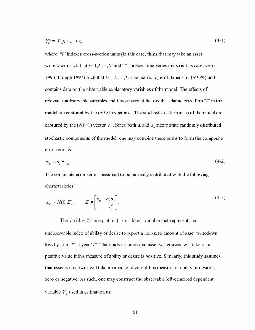

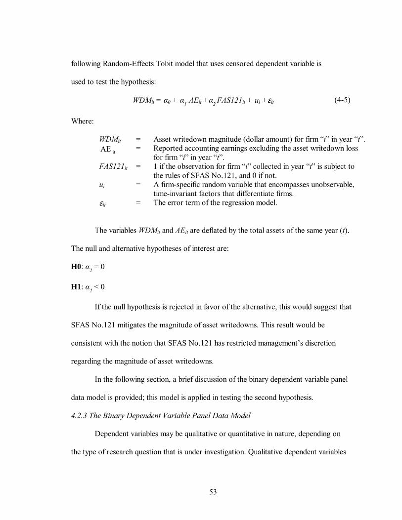

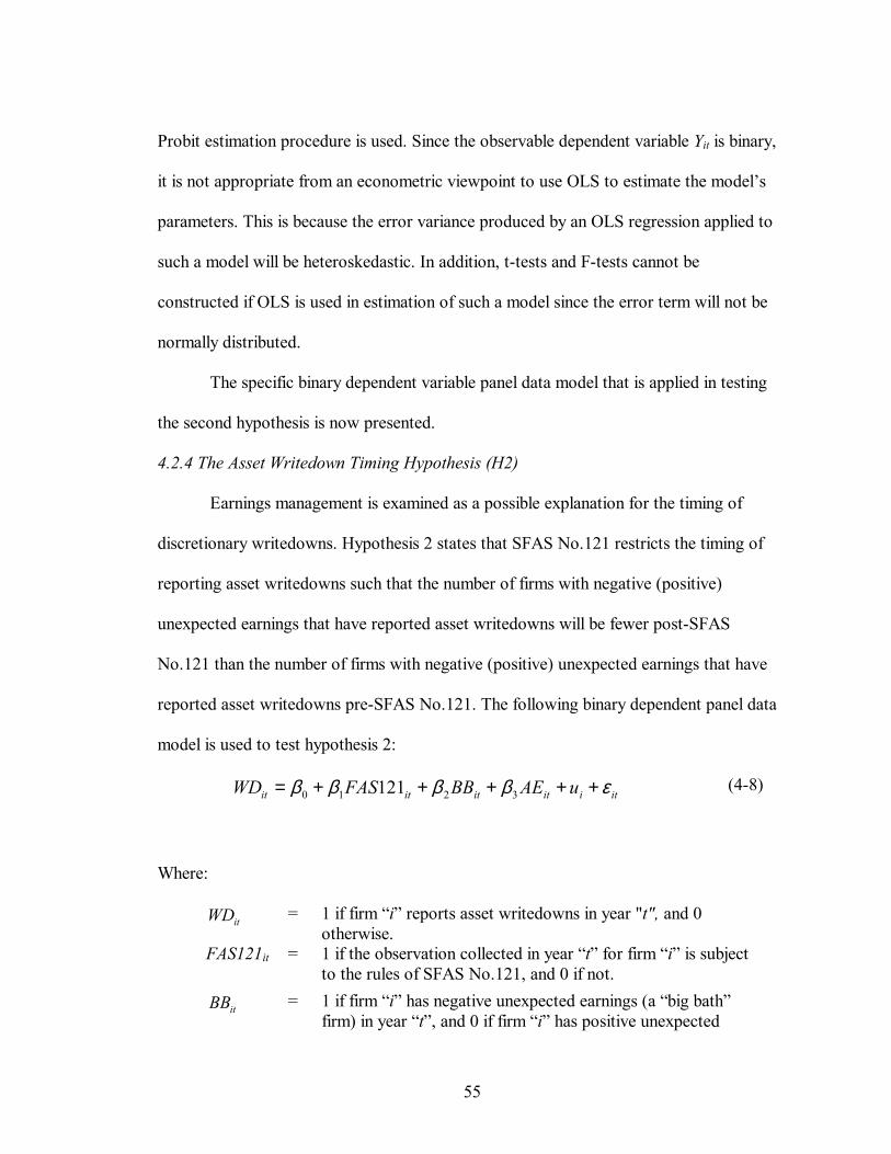
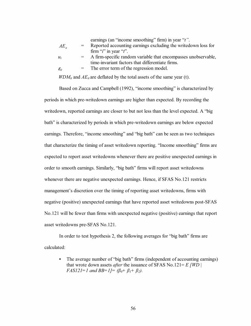


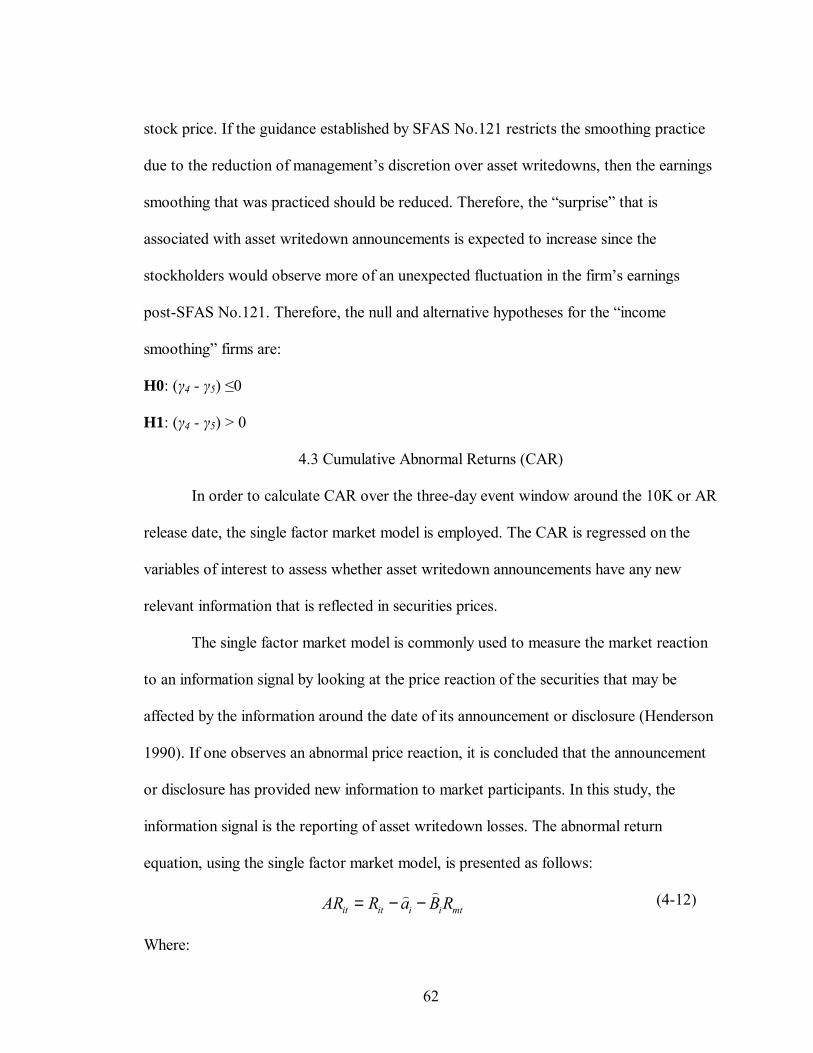


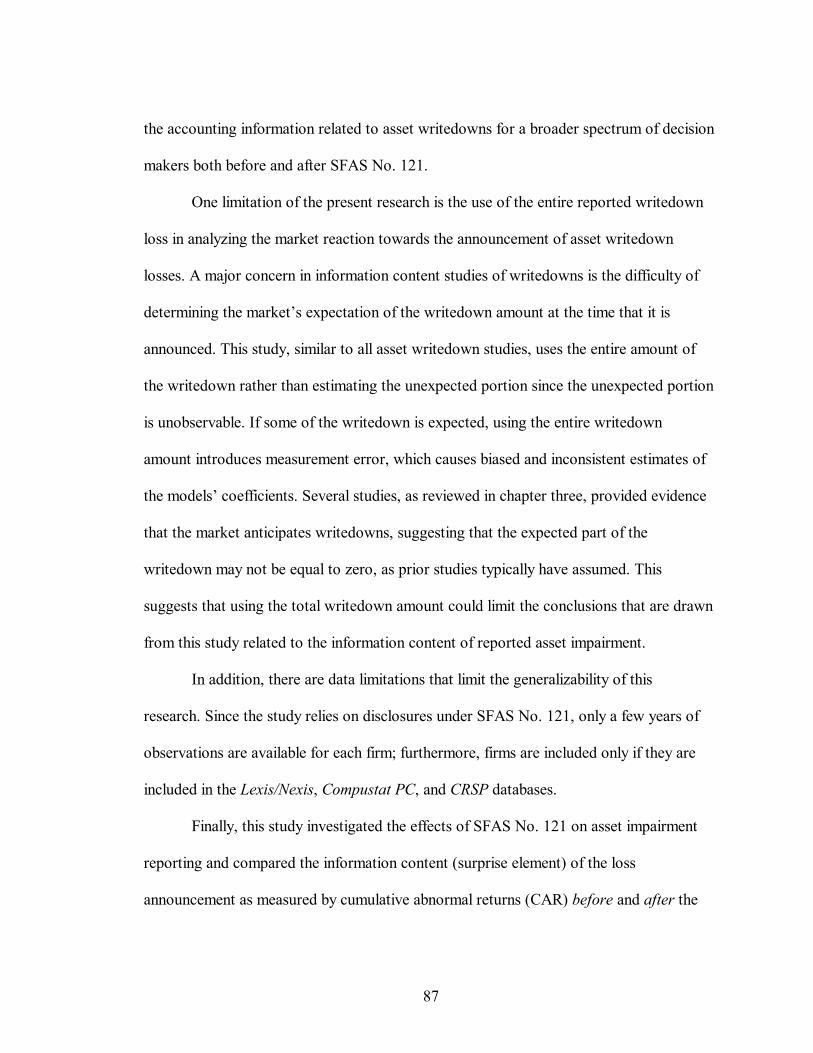


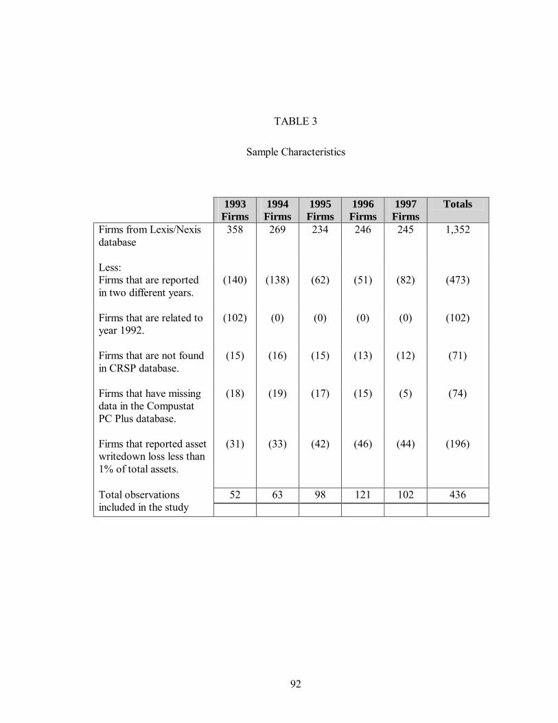
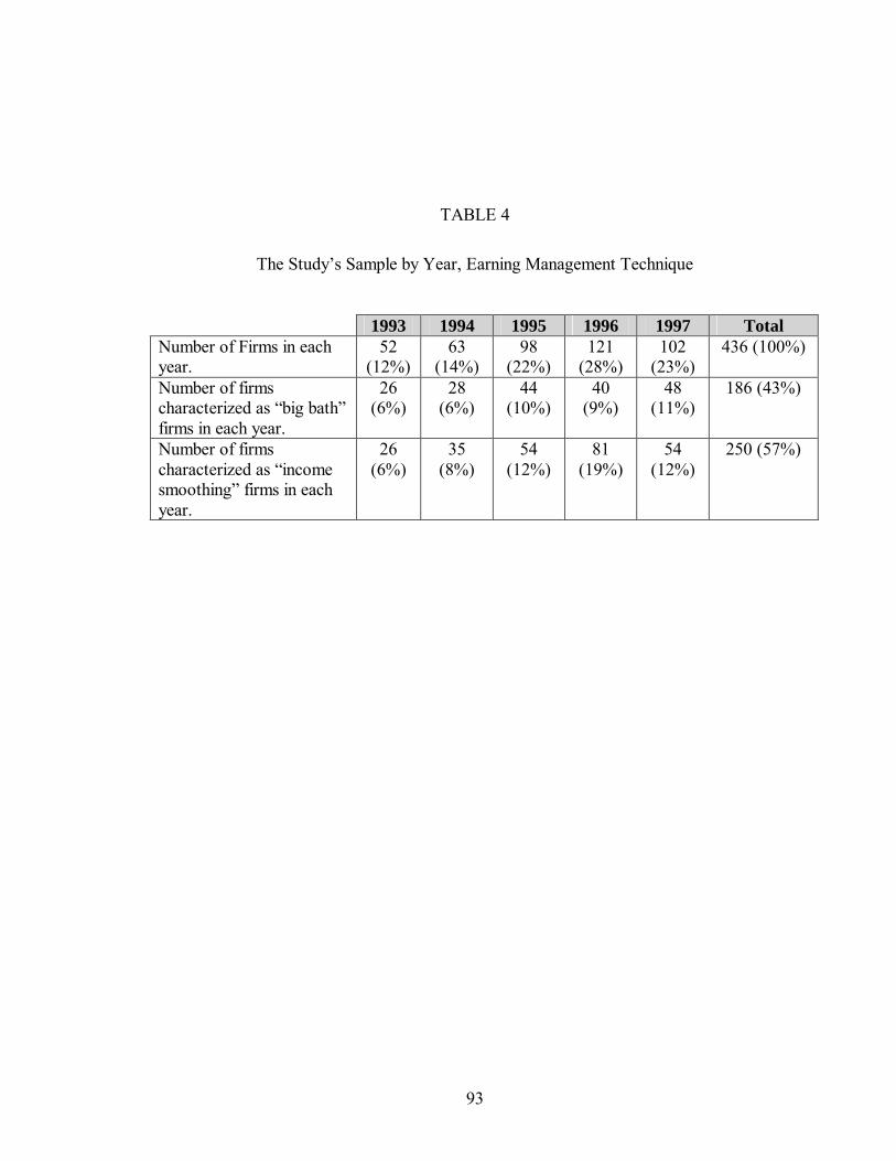

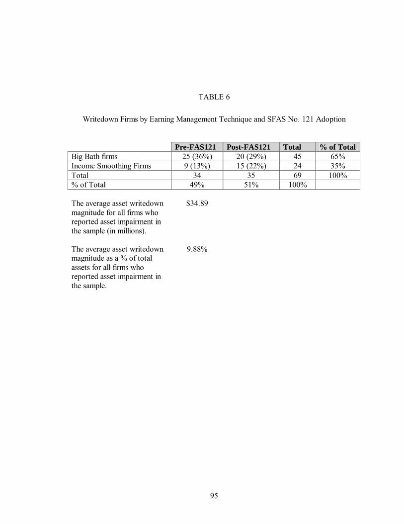


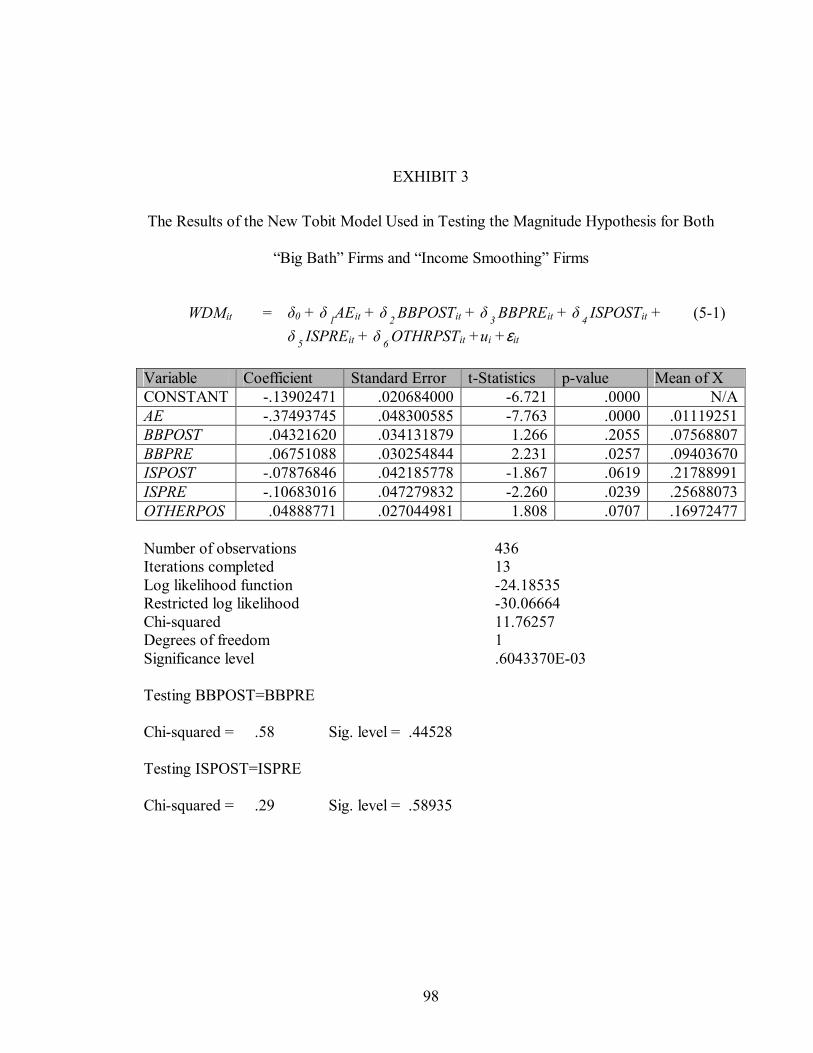
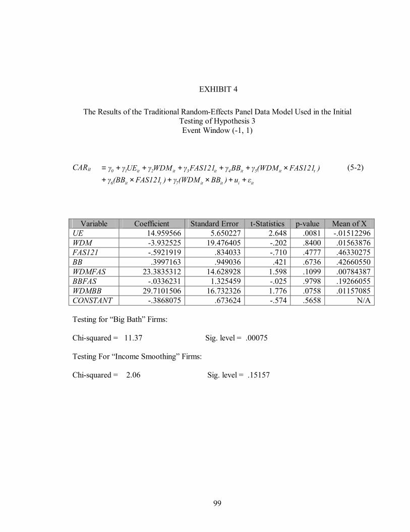

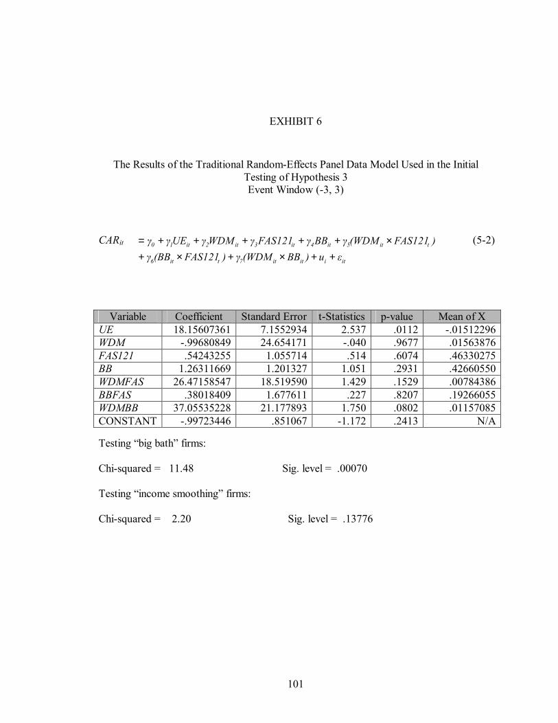


![Sfas dts help final[1]](https://static.documents.pub/doc/80x56/55858fb0d8b42aca7b8b46d5/sfas-dts-help-final1.jpg)


