1

1

AN INVESTIGATION ON THE USE OF GPS FOR DEFORMATION MONITORING IN OPEN PIT MINES

Jason Bond, Donghyun (Don) Kim, Richard B. Langley and Adam Chrzanowski Department of Geodesy and Geomatics Engineering, University of New Brunswick

ABSTRACT

Deformation monitoring in an open pit mine poses some interesting challenges. Due to limitations with classical geodetic techniques, the Canadian Centre for Geodetic Engineering (CCGE) at UNB has decided to pursue augmenting its fully-automated deformation monitoring system with GPS. Just as there are limitations with classical techniques of deformation monitoring in an open pit mine, so too are there constraints placed on the use of GPS. High-performance GPS RTK software has been developed within the Geodetic Research Laboratory (GRL) at the University of New Brunswick (UNB). This software was initially designed for gantry crane auto-steering. Naturally, the GRL and CCGE have combined efforts to attempt to achieve the required precision for this application. As a first step, tests of a modified version of the GPS RTK software have been carried out at Highland Valley Copper Mine in British Columbia, Canada. These results are compared with results attained from Trimble Total Control and UNB’s DIPOP GPS processing software. Because the stability of the benches is of primary concern, the GPS vertical component solution is of particular interest. This paper introduces the approach taken at UNB to address high precision requirements in a constrained environment. Technical and scientific aspects of the UNB RTK software, especially in handling two predominant errors (residual tropospheric zenith delay and multipath) at the mine, are discussed. Remaining issues that need to be addressed in order to meet the needs of this application are also presented.

1 INTRODUCTION

When monitoring deformations by means of precision surveys, several reference stations are typically setup against which the displacements of object points are calculated. To ensure that sound conclusions are made based upon analysis of the displacements, it is necessary to ensure that the reference stations are, in fact, stable. Otherwise, incorrect conclusions will be drawn based upon misinterpretations. To obtain the displacements of the object points, the stability of the reference points must be confirmed and any unstable points identified.

Recently, the Canadian Centre for Geodetic Engineering (CCGE) at UNB has developed a fully automated system for monitoring steep embankments [Duffy et al., 2001; Wilkins et al., 2003], and slope stability. The system utilizes robotic total stations (RTS) and a number of retroreflecting prisms mounted on the monitored object. In order to reduce pointing errors and, particularly, effects of atmospheric refraction to the millimetre level, the distances to the target prisms must be within a few hundred metres. This means that in large open pit mines the robotic total stations must be placed at the bottom of the pit and as near as possible to the monitored slope. This poses a problem of having RTSs located in an unstable environment with a limited visibility to the stable reference targets located outside the rim of the pit. The current work at CCGE concentrates on combining RTSs with GPS, into a hybrid monitoring system in which GPS would control the stability of the RTS. To make such hybrid system useful for high precision and fully automated monitoring of deformations, two requirements must be fulfilled:

• Accuracy of controlling the stability of the RTSs must be within a few millimetres at the 95% confidence level (particularly in height changes), and

• RTS position corrections must be derived from GPS data in a fully automated mode. This purpose of this investigation, then, is to address the first problem, i.e. how to achieve the millimetre accuracy in GPS determination of displacements.

2

2

2 LOCAL DEFORMATION MONITORING IN AN OPEN PIT MINE USING GPS

Deformation monitoring in an open pit mine through the use of GPS poses some interesting challenges. To attain high-precision positioning results, it is necessary to identify error sources that impact the quality of GPS measurements. Some of the error sources have systematic characteristics while others have quasi-random characteristics. For example, the effects of cycle slips and receiver clock jumps can be easily captured either in the measurement or parameter domain due to their systematic characteristics. Their systematic effects on the carrier-phase measurements can be almost completely removed once they are correctly identified. On the other hand, multipath, diffraction, ionospheric scintillation, etc. have temporal and spatial characteristics which are more or less quasi-random. These quasi-random errors cannot be completely eliminated. Instead, they must be handled using a rigorous mathematical approach to isolate their effects as much as possible from parameter estimates.

It is important to know if error effects can be mitigated by means of processing techniques such as forming the single difference (SD) or double difference (DD) observables. If it is known that some errors cannot be removed completely, it is important to determine whether or not their residual effects are negligible. Failure to account for non-negligible residual effects will result in a deterioration of the quality of the measurements and consequently, the quality of positioning results. For deformation monitoring in an open pit mine, the following errors are deemed significant:

• Residual tropospheric delay and • Multipath.

2.1 Residual Tropospheric Delay

When processing GPS data, a value for the tropospheric delay is typically predicted using empirical models which, in general, must be provided with measured or standard values of ambient temperature, pressure and relative humidity. Unfortunately, even with accurate values, these models rarely predict the true delay with a high degree of accuracy. The residual tropospheric delay is the remaining part of the tropospheric delay not predicted by empirical models. It can be the largest remaining error source in dual-frequency precision positioning [Collins and Langley, 1997]. Like many other spatially-dependent error sources, the effects of the tropospheric delay are usually negligible in relative positioning in short-baseline environments. If there are large height differences (or rapid height variations in kinematic positioning) between the reference and rover antennas, differential tropospheric delays may be significant. If significant differences in meteorological conditions exist between stations, tropospheric delays will not cancel through double-differencing. To more concretely define the term significant, consider the expression for zenith tropospheric delay [Langley, 1995]:

dztrop = rs-ra| ∫ [n(r) – 1]dr

= 10-6 rs-ra| ∫ [N(r)]dr (1)

Where: n = the refractive index N = the refractivity (N= 106 (n-1)) r = the geocentric radius rs = radius of Earth’s surface ra = radius of the top of the neutral atmosphere

To determine the impact of a height difference on relative GPS positioning solutions, consider two stations that have a height difference of ∆h m. We can approximate the tropospheric delay at each station as:

dz

trop1 = 10-6 x N1 x pathlength1 dz

trop2 = 10-6 x N2 x (pathlength1 + ∆h)

3

3

Differencing the two equations yields:

∆dz

trop1-2 = 10-6 x (∆N x pathlength1) + (N2 x ∆h) [m] (2) Over a short baseline, the first term should cancel out, since the troposphere over the master and rover stations will be nearly the same and ∆N will equal 0. The differential tropospheric delay, then, will be approximately equal to the refractive index over the extra path length travelled to station 2, multiplied by this extra path length (or, equivalently, the height difference). If, for example, ∆h = 500 m and N2 = 10-6 x 300, then ∆dz

trop1-2 = 0.150m. Refractivity may be approximated by the Smith-Weintraub equation [Smith and Weintraub]:

N = 77.6 x P/T + 3.73E5 x e/T2 (3) Where: P = pressure of the parcel of air [mbar] T = temperature of the parcel of air [K] e = water vapour The first and second terms of Equation 4 are commonly referred to as the dry and wet components of refractivity [Langley, 1995]. About 90% of the magnitude of the tropospheric delay arises from the dry component, while the remaining 10% is associated with the wet component [Rizos, 2001]. For simplification purposes we will focus on the dry component. A height-dependent function for the signal refractivity along the signal path was developed by Helen Hopfield [Seeber, 1993]: Nd(h) = Nd0 x ((Hd – h)/ Hd)4 (4) Where: Nd0 = the surface refractivity (dry component of Equation 3) H = the height above the surface [m] Hd = 40136 + 148.72(T – 273.16), T [K], (as determined by Hopfield) Assuming standard conditions (P = 1013.25 mbar, T = 293.15 K), then Nd0 = 268.2. Based on the assumption that temperature decreases with height as 6.71 Cº /km [Seeber, 1993], then the temperature at a height of 500m above the surface would be about 296.50 K, Hd = 43607.1248, Nd(500) =256.1, and ∆dz

trop1-2 = 0.128m! Beutler et al. [1988] have shown that the effect of the differential troposphere on local GPS networks

leads to a relative height error that can be approximated to first order as

∆he = ∆dztrop secΨmax (5)

Where:

∆dztrop = the difference in zenith delay between co-observing stations

Ψmax = the maximum zenith angle observed Neglect of the differential troposphere leads to approximately 3 to 5 mm relative height error for every millimetre change in zenith delay between stations for Ψmax = 70-80º. Differential tropospheric delay must be accounted for if millimetre level precisions are to be attained. 2.2 Multipath

From the simplest approach of selecting an optimal antenna location, to the most complicated receiver technology, a number of multipath mitigation techniques have been proposed to mitigate the effects of multipath in GPS code and carrier phase measurements. Although recent receiver technologies have significantly improved medium and long delay multipath performance, multipath mitigation techniques for

4

4

short delays (due to close-by reflectors) are not at the same level [Weill, 2003], [Braasch and Van Dierendonck, 1999].

Multipath experienced at two or more independent antennas is spatially correlated within a small area where each antenna is under the same multipath environment (that is, the antennas are in the vicinity of large obstacles). Except for this case, multipath is not spatially correlated. Therefore, the effects of multipath can be significant in relative positioning (even on short-baselines) and cannot be cancelled by the double-differencing operation. Multipath due to specular reflection on a smooth surface shows apparent daily correlation due to repeated satellite-receiver-reflecting object geometry. However, multipath due to diffraction (reflection from the edges or corners of the reflecting objects) and diffusion (reflection from rough surfaces) does not usually show such an apparent day-to-day correlation. Typically, in open pit mine environments, multipath due to diffraction and diffusion occurs more often than specular reflection. Therefore, day-to-day correlation analysis can not typically be used to mitigate multipath effects.

3 UNB APPROACH The challenge in attaining sub-centimetre accuracy positioning at the open pit mine comes from trying

to mitigate the: 1. Residual (unmodelled) tropospheric delay due to extreme height differences between two

GPS monitoring stations. 2. Short delay multipath, especially that due to diffraction and diffusion whose patterns do not

repeat daily and therefore cannot be easily removed by data “stacking” or other means. 3.1 UNB3 Tropospheric Delay Model

The original definition of the UNB3 composite model is based on the zenith delay algorithms of Saastamoinen [1973], the mapping functions of Niell [1996], and a table of surface atmospheric values derived from the U.S. 1966 Standard Atmosphere Supplements. The kernel of the UNB3 model is a look-up table of five values of atmospheric parameters that vary with respect to latitude and day-of-year. Linear interpolation is applied between latitudes and a sinusoidal function of the day-of-year attempts to model the seasonal variation. The parameters are total pressure, temperature and water vapour pressure at mean-sea-level, and two lapse rate parameters for temperature and water vapour. The lapse rates are used to scale the pressures and temperature to the user’s altitude. The typical formulation of the tropospheric delay is described as:

( ) ( )

( ) ( ) ( ) ( ),

( ) ( )

k z ki i iz z zi i i

z k z kk i i i ii z z

i i

T t m

t t hyd t wet

t hyd m hyd t wet m wetm

t hyd t wet

= ⋅

= +

⋅ + ⋅=

+

(6)

where at the antenna of receiver i, the delay on the signal from satellite k is a function of the delays in the zenith direction caused by the atmospheric gases in hydrostatic equilibrium and by those gases not in hydrostatic equilibrium (primarily water vapour), ( )z

it hyd and ( )zit wet respectively; and their mapping

functions, ( )kim hyd and ( )k

im wet respectively. The mapping functions are usually described as functions of the satellite elevation angle. By introducing a residual zenith delay parameter z

ir in the formulation and assuming no errors in the mapping function, we have

( )k z z ki i i iT t r m= + ⋅ . (7)

The differential tropospheric delay between satellites k and l and stations i and j is given by:

5

5

( ) ( )( )( ) ( )( ).

kl l k l kij j j i i

z z l k z z l kj j j j i i i i

T T T T T

t r m m t r m m

= − − −

= + − − + − (8)

Fixing the tropospheric delay at the reference station and estimating the relative delay z

jr at the secondary station gives with partial derivatives:

klij l k

j jzj

Tm m

r∂

= −∂

. (9)

3.2 Multipath Mitigation The main approach employed to mitigate multipath is using an optimal inter-frequency carrier phase linear combination of the L1 and L2 observations [Kim and Langley, 2001]. A generic inter-frequency carrier phase linear combination of the L1 and L2 observations is given as:

( )1 1 2 2 1 2 1 1 1 2 2 2 1 1 2 2k k k k k N k N k kρ λ λ ε εΦ + Φ = + + + + + (10)

where Φ is the measured carrier phase (m), ρ is the geometric range from antenna phase centre to GPS satellite; λ is the carrier wavelength (m/cycle); N is integer ambiguity (cycle); ε includes all other biases and errors such as multipath, measurement noise, etc.; and subscripts “1” and “2” indicate L1 and L2 values, respectively. Since we can divide the term 1 2k k+ combined with ρ on both sides, an equivalent mathematical expression holds as:

1 2 1k k+ = . (11)

Obtaining an optimal inter-frequency carrier phase linear combination of the L1 and L2 observations is coincident with solving K1 and K2 in the following matrix equation:

( )min , with ,+ =T1 2K1, K2

KQK K K I (12)

where [ ]= 1 2K K K ; Q is the variance-covariance matrix of the combined L1 and L2 observations; and I is an identity matrix. Unfortunately, an analytical solution for Eq. (7) is not available because the number of unknown parameters is much larger than that of measurements. Alternatively, we are interested in finding K1 and K2 which guarantee an upper bound as:

( )≤ +TL1 L2

1KQK Q Q2

. (13)

Eq. (8) means that the noise level of an optimal combination is always smaller than that of L1 or L2. One example of such solutions is given as:

( )( ) .

= +

= +

-11 L1 L2 L2

-12 L1 L2 L1

K Q Q Q

K Q Q Q (14)

Another approach to mitigate multipath is based on a smoothing process such as the sequential least-squares estimation. Since the time constant of multipath is usually shorter than an hour, for example, the parameter estimates sequentially estimated over one hour session may be less contaminated by multipath.

6

6

4 DATA COLLECTION AND PROCESSING

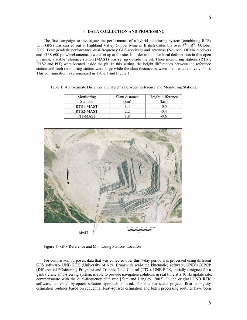
The first campaign to investigate the performance of a hybrid monitoring system (combining RTSs with GPS) was carried out at Highland Valley Copper Mine in British Columbia over 4th - 8th October 2002. Four geodetic performance dual-frequency GPS receivers and antennas (NovAtel OEM4 receivers and GPS-600 pinwheel antennas) were set up at the site. In order to monitor local deformation in this open pit mine, a stable reference station (MAST) was set up outside the pit. Three monitoring stations (RTS1, RTS2 and PIT) were located inside the pit. In this setting, the height differences between the reference station and each monitoring station were large while the slant distance between them was relatively short. This configuration is summarized in Table 1 and Figure 1.

Table 1. Approximate Distances and Heights Between Reference and Monitoring Stations.

Monitoring Stations

Slant distance (km)

Height difference (km)

RTS1-MAST 1.4 -0.5 RTS2-MAST 2.2 -0.4 PIT-MAST 1.8 -0.6

Figure 1 GPS Reference and Monitoring Stations Location

For comparison purposes, data that was collected over this 4-day period was processed using different GPS software- UNB RTK (University of New Brunswick real-time kinematic) software, UNB’s DIPOP (DIfferential POsitioning Program) and Trimble Total Control (TTC). UNB RTK, initially designed for a gantry crane auto-steering system, is able to provide navigation solutions in real time at a 10 Hz update rate, commensurate with the dual-frequency data rate [Kim and Langley, 2002]. In the original UNB RTK software, an epoch-by-epoch solution approach is used. For this particular project, float ambiguity estimation routines based on sequential least-squares estimation and batch processing routines have been

MAST

7

7

implemented. The main reason for this modification was poor satellite visibility within the confines of the mine. In this initial assessment, real-time operation was not attempted. Data collected by the GPS receivers was post-processed. DIPOP is a scientific GPS differential positioning program that has been recently adorned with a Windows interface- FACE. Although more time consuming to use than commercial packages, DIPOP allows much more control over processing options. In particular, DIPOP allows the user to estimate tropospheric parameters, which should lead to an improved vertical solution. Trimble Total Control is a processing package for GPS and conventional survey measurement data. Recent comparisons of commercial software at UNB indicate that TTC is one of the most flexible when it comes to processing options, and its solutions show a high degree of repeatability.

Data was collected at 1 Hz. Session lengths were varied to determine the optimal observation period. It may be possible to attain millimetre level results after a day’s observations, however, this may not be very practical for “near real-time” deformation monitoring. It was determined that a session length of at least 3 hours is required to produce the repeatability of solutions desired.

5 TEST RESULTS

Height solutions using the modified UNB RTK software (albeit in a post-processing mode) are illustrated in Figure 2. The data recorded over 4 consecutive days was spliced into 96 one-hour sessions and processed independently. Northing, easting and height components of RTS1, RTS2 and PIT from MAST were estimated. A maximum to minimum spread of about 5 cm can be seen. Moving average values over 12 and 24 hours were also computed, which brings the range down to about 2 cm.

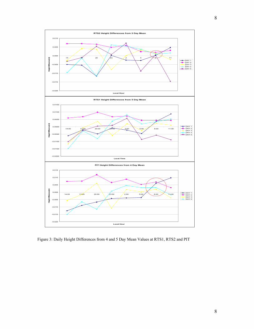
Height solutions were calculated after each 3 hour observation period using TTC, so that 8 solutions were attained per day. The results are presented in Figures 3. A maximum to minimum spread of just over 2 cm can be seen Because of length of time required to process data in DIPOP, only the first 12 hours of the PIT and RTS1 stations were processed. The results are shown in Figure 4. A similar 2 cm range can be seen.

Figure 2. Positioning solutions (height) for individual one-hour session over four consecutive days (left) and moving averages of them over 12 and 24 hours (right).

8

8

RTS2 Height Differences from 5 Day Mean

-0.020

-0.015

-0.010

-0.005

0.000

0.005

0.010

14 17 20 23 2 5 8 11

Local Hour

Heigh

t Diff

eren

ce [m

]

DAY 1DAY 2 DAY 3DAY 4DAY 5

RTS1 Height Differences from 5 Day Mean

-0.0200

-0.0150

-0.0100

-0.0050

0.0000

0.0050

0.0100

0.0150

14:00 17:00 20:00 23:00 2:00 5:00 8:00 11:00

Local Time

Heigh

t Diff

eren

ce [m

]

DAY 1DAY 2DAY 3DAY 4DAY 5

PIT Height Differences from 4 Day Mean

-0.020

-0.015

-0.010

-0.005

0.000

0.005

0.010

0.015

14:00 17:00 20:00 23:00 2:00 5:00 8:00 11:00

Local Hour

Heigh

t Diff

eren

ce [m

]

DAY 1DAY 2DAY 3DAY 4

Figure 3: Daily Height Differences from 4 and 5 Day Mean Values at RTS1, RTS2 and PIT

9

9

RTS2 Height Differences from 12 Hour Mean

-0.012

-0.010

-0.008

-0.006

-0.004

-0.002

0.000

0.002

0.004

0.006

0.008

13.000 15.000 17.000 19.000 21.000 23.000 25.000

Local Hour

Heigh

t Differen

ce [m

]

Day 1

Pit Height Differences from 12 Hour Mean

-0.01

-0.008

-0.006

-0.004

-0.002

0

0.002

0.004

0.006

0.008

13 15 17 19 21 23 25

Local Hour

Heigh

t Differen

ce [m

]

Day 1

Figure 4: Height Differences from 12 Hour Mean, Day 1 at RTS2 and PIT

6 DATA ANALYSIS

Since the monitoring stations are located in the pit, the visibility of GPS satellites at the stations is severely limited by surrounding terrain. At PIT, for example, natural elevation cut-off angles due to the open pit environment range from 15 to 35 degrees (Figure 5, left). Consequently, reduced satellite visibility leads to poor satellite geometry, which in turn causes degraded GPS positioning solutions. Large dilution of precision (DOP) values confirm this aspect in Figure 5 (right), where x-axes in the first three panels are given in hour units in local time and the bottom panel shows that fewer than 7 satellites are available over about 80% of the day.

Figure 5. Skyplot over 24 hours at PIT (left) and the number of satellites and (horizontal and vertical) DOP values (right). Elevation cut-off angle due to the open-pit environment ranges from 15 to 35 degrees.

10

10

Although the situations at RTS1 and RTS2 are slightly better than at PIT as illustrated in Figure 6, satellite geometry at these two stations is quite similar to that at PIT. As a result, all three stations provided very challenging situations in trying to attain sub-centimetre level, high precision positioning solutions from the collected data.

Figure 6. Mean number of visible satellites for individual one-hour session over 24 hours. 6.1 Tropospheric Delay Like many other spatially-dependent error sources, the effects of the tropospheric delay are usually negligible in relative positioning under short-baseline environments. However, as illustrated in Figure 4, the effects can be significant and cannot be cancelled by the double-differencing operation if the height difference between two stations is large. To justify such a case in this application, the DD tropospheric delay observables were used:

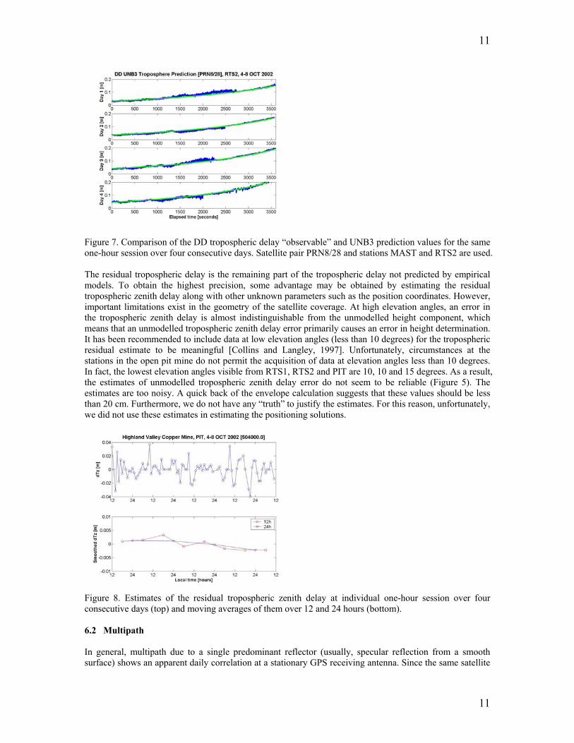
1 1T̂ Nρ λ∆∇ = ∆∇Φ −∆∇ − ∆∇ , (15) where ∆∇ represents the DD operation. T̂∆∇ is a compound error including the tropospheric delay, satellite orbit error, ionospheric delay, multipath, receiver system noise, etc. In the test setup (i.e., short-baseline), we can expect that the DD tropospheric delay will be predominant in Eq. (10). Then, we compared the DD tropospheric delay “observable” (noisy curves in a dark color) with UNB3 prediction values (smooth curves in a light color) for the satellite pair of PRN 8 and 28 at RTS2 over the same one-hour session during four consecutive days. As depicted in the figure, an order of 20 centimetres in the changes of the DD tropospheric delay occurs over one hour, which confirms that the effects of tropospheric delay in the DD measurements are significant. Also, the figure shows that the UNB3 tropospheric delay model performs very well in this application. Unless the effects of tropospheric delay are removed from the carrier-phase measurements, therefore, ambiguity resolution and cycle-slip correction can easily fail.

11

11

Figure 7. Comparison of the DD tropospheric delay “observable” and UNB3 prediction values for the same one-hour session over four consecutive days. Satellite pair PRN8/28 and stations MAST and RTS2 are used. The residual tropospheric delay is the remaining part of the tropospheric delay not predicted by empirical models. To obtain the highest precision, some advantage may be obtained by estimating the residual tropospheric zenith delay along with other unknown parameters such as the position coordinates. However, important limitations exist in the geometry of the satellite coverage. At high elevation angles, an error in the tropospheric zenith delay is almost indistinguishable from the unmodelled height component, which means that an unmodelled tropospheric zenith delay error primarily causes an error in height determination. It has been recommended to include data at low elevation angles (less than 10 degrees) for the tropospheric residual estimate to be meaningful [Collins and Langley, 1997]. Unfortunately, circumstances at the stations in the open pit mine do not permit the acquisition of data at elevation angles less than 10 degrees. In fact, the lowest elevation angles visible from RTS1, RTS2 and PIT are 10, 10 and 15 degrees. As a result, the estimates of unmodelled tropospheric zenith delay error do not seem to be reliable (Figure 5). The estimates are too noisy. A quick back of the envelope calculation suggests that these values should be less than 20 cm. Furthermore, we do not have any “truth” to justify the estimates. For this reason, unfortunately, we did not use these estimates in estimating the positioning solutions.

Figure 8. Estimates of the residual tropospheric zenith delay at individual one-hour session over four consecutive days (top) and moving averages of them over 12 and 24 hours (bottom). 6.2 Multipath In general, multipath due to a single predominant reflector (usually, specular reflection from a smooth surface) shows an apparent daily correlation at a stationary GPS receiving antenna. Since the same satellite

12

12

constellation geometry repeats about 4 minutes in advance each day, it is easy to see the same pattern repeated about 4 minutes earlier each day from the multipath observables as long as the receiving antenna remains stationary. However, multipath due to diffraction and diffusion may not show such an apparent daily correlation. Diffraction and diffusion (similar to multiple specular reflections) can easily change the scenario involving the reflecting objects. As a result, a GPS receiver may track the composite signal of a direct and (multiple) reflected(s) signal with different multipath characteristics every day. Figure 6 illustrates that the effects of multipath at the MAST and PIT stations are not correlated daily. The figure shows the DD residuals for satellite pair PRN 3/18 and stations MAST and RTS2.The residuals are dominated by multipath, receiver noise, and any unmodelled effects. For this reason, we did not use the technique utilizing the repeatability of multipath at stationary stations (“stacking”) to mitigate multipath in the measurements. Alternatively, we used a smoothing process (i.e., sequential least-squares estimation over one hour) and an optimal inter-frequency linear combination of L1 and L2 to reduce the effects of multipath in the measurements.

Figure 6. Multipath observables (DD residuals) at the same one-hour session over four consecutive days.

7 CONCLUDING REMARKS

Considering the requirement of a few millimetres accuracy at the 95% confidence level (particularly in height changes) for local deformation monitoring at an open pit mine, there is still progress to be made to meet the requirement. We have faced two main issues during the first measurement campaign. First, we did not have “truth” to validate our approach. One example, which may lead us to draw misinterpretations and incorrect conclusions, is depicted in Figure 2 and 3. The height solutions of the second day seem to be significantly different from those of the other three days. Furthermore, the height solutions of all three stations RTS1, RTS2 and PIT with respect to MAST seem to be commonly affected by some errors. Therefore, we can conclude that something may have happened at MAST during the second day. Unfortunately, we have nothing to validate this conclusion from the first campaign. Second, the geometry of the satellite coverage in the open pit prohibits us from obtaining the highest precision. Since we struggle with a few millimetres accuracy, we need to estimate the residual tropospheric zenith delay along with unknown parameters such as the position components. Unfortunately, circumstances at the stations do not permit us to obtain data at elevation angles less than 10 degrees. As a result, the estimates of unmodelled tropospheric zenith delay error seem not to be fully reliable.

In order to meet the requirements for this project, further research will be performed. At the present time, the use of pseudolites for deformation monitoring is being investigated. The use of pseudolites should address the issue of limited satellite availability. A second measurement campaign is being planned to collect another set of data. Anomalies (data gaps in the observation files or a possible change in position of the MAST station) hinder sound analysis of the current data set. During this second campaign, meteorological data will be collected in an attempt to more accurately correlate tropospheric effects with

13

13

solution variations. As well, RTSs will be used to monitor the stability of the GPS stations to serve as “truth”.

ACKNOWLEDGEMENTS The research conducted in this paper was made possible through the assistance of the Atlantic Innovation Fund and the Natural Sciences and Engineering Research Council of Canada. The CCGE and GRL gratefully acknowledge their contributions.

REFERENCES Beutler, G., I. Bauersima, W. Gurtner, M. Rothacher, T. Schildknecht, and A. Geiger (1988). “Atmospheric

refraction and other important biases in GPS carrier phase observations.” In Atmospheric Effects on Geodetic Space Measurements, Monograph 12, School of Surveying, University of New South Wales, Kensington, N.S.W., Australia, pp.15-43.

Braasch, M. S. and A. J. Van Dierendonck (1999). “GPS receiver architectures and measurements.” Proceedings of the IEEE, Vol. 87, No. 1, January, pp. 48-64.

Collins, J.P. and R.B. Langley (1997). “Estimating the residual tropospheric delay for airborne differential GPS positioning.” Proceedings of ION GPS-97, the 10th International Technical Meeting of the Satellite Division of the Institute of Navigation, Kansas City, MO, 16-19 September 1997, pp. 1197-1206.

Duffy, M., C.Hill, C, Whitaker, A. Chrzanowski, J. Lutes, G. Bastin (2001). “An automated and integrated monitoring program for Diamond Valley Lake in California”. Proceedings (CDRom) of the 10th Int. Symposium on Deformation Measurements (Metropolitan Water District of S. California), Orange, CA, March 19-22. Available at: http://rincon.gps.caltech.edu/FIG10sym/

Kim, D. and R.B. Langley (2001). “Mitigation of GPS carrier phase multipath effects in real-time kinematic applications.” Proceedings of ION GPS 2001, 14th International Technical Meeting of the Satellite Division of The Institute of Navigation, Salt Lake City, UT, 11-14 September, pp. 2144-2152.

Kim, D., R.B. Langley, and S. Kim (2002). “Shipyard Giants. High-precision crane guidance.” GPS World, Vol. 13, No. 9, September, pp. 28-34.

Langley, R.B., (1995). Propagation of the GPS Signals. Chapter 3 from GPS for Geodesy, Delft, Netherlands, 26 March 1- April 1995.

Niell, A.E. (1996). “Global mapping functions for the atmosphere delay at radio wavelengths.” Journal of Geophysical Research, Vol. 101, No. B2, pp 3227-3246.

Rizos, C. 2001. Principles and Practice of GPS Surveying. http://www.gmat.unsw.edu.au/snap/gps/gps_survey/principles_gps.htm, 09 February 2003. Saastamoinen, J. (1973). “Contributions to the theory of atmospheric refraction.” In three parts. Bulletin

Géodésique, No. 105, pp. 279-298; No. 106, pp.383-397; No. 107, pp. 13-34. Seeber, G., 1993. Satellite Geodesy: Foundations, Methods, and Applications. Walter de Gruyter, Berlin,

NewYork, 1993. Smith, E.K. and S. Weintraub, (1953). “The constants in the equation of atmospheric refractive index at

radio frequencies.” Proceedings of the Institute of Radio Engineers, Vol. 41, No. 8, pp. 1035-1037. Weill, L.R. (2003). Multipath Mitigation. How Good Can It Get with New Signals. GPS World Innovation

Column, June 2003. http://www.gpsworld.com/gpsworld Wilkins, R., G. Bastin, A. Chrzanowski, W. Newcomen and L. Shwydiuk (2003) “A fully automated

system for monitoring pit wall displacements” Presented at SME annual conference 2003, Cincinnati, Feb. 24-26, 2003 (available at http//:ccge.unb.ca)