Page 1
1
An involute spiral that matches G2 Hermite data in the plane
by
T. N. T. Goodmana, D. S. Meekb, and D. J. Waltonc
Abstract
A construction is given for a planar rational Pythagorean hodograph spiral which
interpolates any two-point G2 Hermite data that a spiral can match. When the curvature at one of
the points is zero, the construction gives the unique interpolant that is the involute of a rational
Pythagorean hodograph curve of the form cubic over linear. Otherwise, the spiral comprises an
involute of a Tschirnhausen cubic together with at most two circular arcs. The constructions are
explicit apart from solving two linear equations in the first case, and at most one quadratic
equation in the second case.
Keywords: rational spirals, G2 Hermite interpolation
1. Introduction
Curves with monotone curvature are called spirals. It is widely accepted that a planar curve
is fair (has a pleasing look) if it has a small number of spiral pieces (Farin, 1997, page 364).
Thus, it is sensible to construct fair planar curves by smoothly piecing together spirals. A curve
is G2 continuous if it, its tangent direction, and its curvature are all continuous (Farin, 1997, page
181). In order to achieve G2 continuity at the joins of neighbouring spirals, it is natural to
consider the problem of interpolating two-point G2 Hermite data by a spiral. A spiral can
interpolate only certain G2 Hermite data, as described in Section 2.3, and such data will be
referred to as admissible G2 Hermite data.
In (Meek, 1992), the authors form a spiral from a clothoid and additional circular arcs that
can match any admissible G2 Hermite data. However their method has the disadvantages that
nonlinear equations involving Fresnel integrals have to be solved, and the clothoid is a
transcendental function which cannot be represented as a NURBS. In a later paper (Meek,
a Department of Mathematics, University of Dundee, Dundee, Scotland, DD1 4HN, e-mail:
[email protected] Corresponding author: Department of Computer Science, University of Manitoba, Winnipeg, Manitoba,
Canada, R3T 2N2, Phone: 1 (204) 474-8681, Fax: 1 (204) 474-7609, e-mail: [email protected] St. Paul's College, University of Manitoba, Winnipeg, Manitoba, R3T 2M6, e-mail: [email protected]
Page 2
2
1998), the authors solve the problem by forming a spiral from a segment of a given spiral
together with circular arcs, but the method still requires the solving of nonlinear equations.
A different approach to the construction of spirals is considered by Haddow and Biard
(Haddou, 1995). They use the fact that the involute of a planar convex curve is a spiral
(Guggenheimer, 1963, page 52). They also use the fact (Pottmann, 1995a) that the involute of a
rational Pythagorean hodograph curve (PH curve) is itself a rational PH curve (see Section 2).
The spirals in (Haddou, 1995) are involutes of PH cubics (also called Tschirnhausen cubics or
T-cubics (Farouki and Sakkalis, 1990)). These involutes are rational PH curves of the form
quartic over quadratic and are termed class 3 curves in (Pottmann, 1995b). It is shown in
(Haddou, 1995) that spirals formed from pairs of such curves will interpolate any admissible G2
Hermite data with non-zero curvatures. However constructing such a spiral requires solving a
nonlinear equation and the case of zero curvature at one end-point is not considered. Note that
(Pottmann, 1995b) studies interpolation by a different class of PH curves, termed class 4 curves,
but spirals are not particularly considered.
A more recent paper (Kuroda and Mukai, 2000) constructs G2 Hermite interpolants using
involutes of circular arcs. For interpolation at n points, a system of 2n nonlinear equations must
be solved. While this involute is apparently appropriate for mechanical systems, it has the
disadvantage of not being representable as a NURBS.
Since a curve interpolating general data would usually have inflection points, any such
curve composed of spirals would necessarily include spirals that have zero curvature at one end-
point. Thus it is important to consider admissible G2 Hermite data involving zero curvature. A
method for constructing an interpolating spiral to any such data is given in Section 3. As in
(Haddou, 1995), the spiral is the involute of a PH curve, but in order to gain zero curvature the
PH curve is rational of the form cubic over linear, and hence the involute is a rational PH curve
of the form quintic over quartic. It is shown that for any admissible G2 Hermite data with zero
curvature at one point, there is a unique interpolating spiral of the above form, and its
computation requires only the solution of two linear equations.
The corresponding G2 Hermite interpolation problem for data with non-zero curvatures is
considered in Section 4. As in (Haddou, 1995) it is seen that a single class 3 curve is not
sufficient, but whereas Haddou and Biard employ a pair of class 3 curves, here a class 3 curve
together with at most two circular arcs is used. This has the disadvantage that three distinct cases
(0, 1, or 2 circular arcs) arise and that makes the theory somewhat inelegant. However, it has the
considerable practical advantage that for the construction one need solve at most one quadratic
equation.
Page 3
3
2. Background
2.1 Notation
The length of a vector p is
p =pxpy
= px
2+ py
2 ,
and the angle of vector p is the counterclockwise angle from the positive x-axis to p (assuming
the tail of p is at the origin). The scalar cross product is
p q = px qy – qx py = ||p|| ||q|| sin ,
where is the signed (counterclockwise is positive) angle from p to q. Using the convention that
all rotations are about the origin, the rotation matrix is
R( ) =cos sin
sin cos
.
2.2 Evolutes and involutes
The evolute of a planar curve is the curve traced by its centres of curvature. The involute of
a planar curve is the curve described by the free end of a string whose other end is attached to the
curve at one point, which is held taut against the curve, and which is wound around the curve.
There is a free parameter in the involute as initially the string can have any length. The evolute of
the involute is the original curve.
Define a convex curve to be a continuous planar curve whose angle of tangent vector is
strictly monotone. The involute of a planar convex curve is a planar spiral (Guggenheimer, 1963,
page 52). For the involute to be G2 continuous, the evolute cannot have a straight line segment as
that would give a jump in the curvature. The evolute can have a cusp (discontinuity in the unit
tangent vector) and still have an involute which is a G2 spiral. A cusp in the evolute will generate
a circular arc in the spiral and the arc will join the neighbouring spiral segments with G2
continuity. In this paper, discontinuities in the unit tangent vector will be used at both ends of the
evolute curve, resulting in a spiral with a circular arc on each end, or at one point in the interior of
the evolute curve, resulting in a circular arc with a spiral on each end.
2.3 Admissible G2 Hermite data
The two-point G2 Hermite data that can be matched by a G2 continuous spiral are referred
to as admissible G2 Hermite data. The restrictions that a spiral imposes on G2 Hermite data are
given in this section. Let the G2 Hermite data be A, B (points), TA, TB (unit tangents), kA, kB
(curvatures). Without loss of generality, 0 kA < kB, and let W be the angle from TA to TB. It
simplifies the discussion to assume that 0 < W < and to use a standard form: namely, A at the
origin, TA along the positive X-axis, and B in the first quadrant (see Figure 1).
Page 4
4
A
kA
BkB
TA
TB
W
Figure 1
Two-point G2 Hermite data in standard form.
One way to show which data a spiral can match is to use the above standard form with W,
kA, kB given and indicate the allowable region for B. The necessary and sufficient conditions that
G2 Hermite data can be matched by a spiral are given in Guggenheimer (1963, page 52).
Examples of the corresponding regions for B are shown in Figures 2 and 4 (Meek and Walton,
1992). Define R and, if kA > 0, define S and L as
R =1
kB
sinW
1 cosW
, S =
1
kA
sinW
1 cosW
, L =
1
kA
1
kB. (2.1)
Define the centre of curvature at B, CB, and if kA > 0, define the centre of curvature at A as
CA =A +1
kAR2
TA , CB = B +
1
kBR2
TB.
2.3.1 kA = 0
Valid B (the region shown in Figure 2) are
B =R+ u1
0
+ v
cosW2
sinW
2
, 0 < u,v < .
Let V be the intersection of BCB extended to meet the Y-axis (see Figure 3). The evolute of
a segment of a spiral is a convex curve lying in the region bounded by the Y-axis, VCB and a ray
from CB parallel to the Y-axis, hereafter called the degenerate triangle VCB. The G2 Hermite data
for a spiral with kA = 0 can be expressed by the degenerate triangle VCB and the curvature kB.
Page 5
5
A
kA = 0
W2
TA
R
B
Figure 2
Allowable region for B for kA = 0.
A TA
WW
B
TB
1kB
CB
V
Figure 3
G2 Hermite data with kA = 0 expressed by degenerate triangle VCB and curvature kB.
2.3.2 kA > 0
Valid B (the region shown in Figure 4) are
B =R+ rsin
1 cos
, 0 < r < L, 0 < <W .
Let V be the intersection of BCB extended to meet the Y-axis (see Figure 5). The evolute
of a segment of a spiral that satisfies the G2 Hermite data in Section 2.3 is a convex curve that
lies in triangle CAVCB and whose arc length is L,
CB CA < L < V CA + CB V (2.2)
Page 6
6
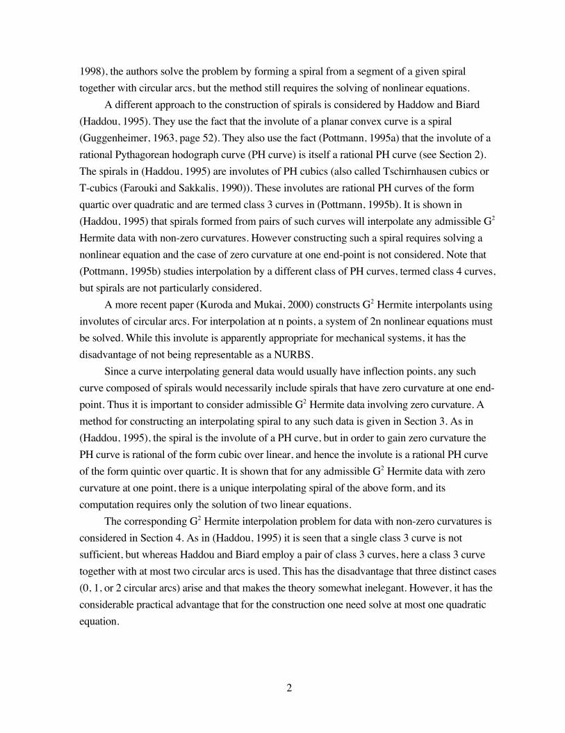
(Guggenheimer, 1963, page 50). The G2 Hermite data for a spiral with kA > 0 can be expressed
by the triangle CAVCB and the curvatures kA and kB.
A
kA > 0
W2
TA
R
S
B
Figure 4
Allowable region for B when kA > 0.
A TA
1kA W
W
B
TB
1kB
CA
CB
V
Figure 5
G2 Hermite data with kA > 0 expressed by triangle CAVCB and curvatures kA and kB.
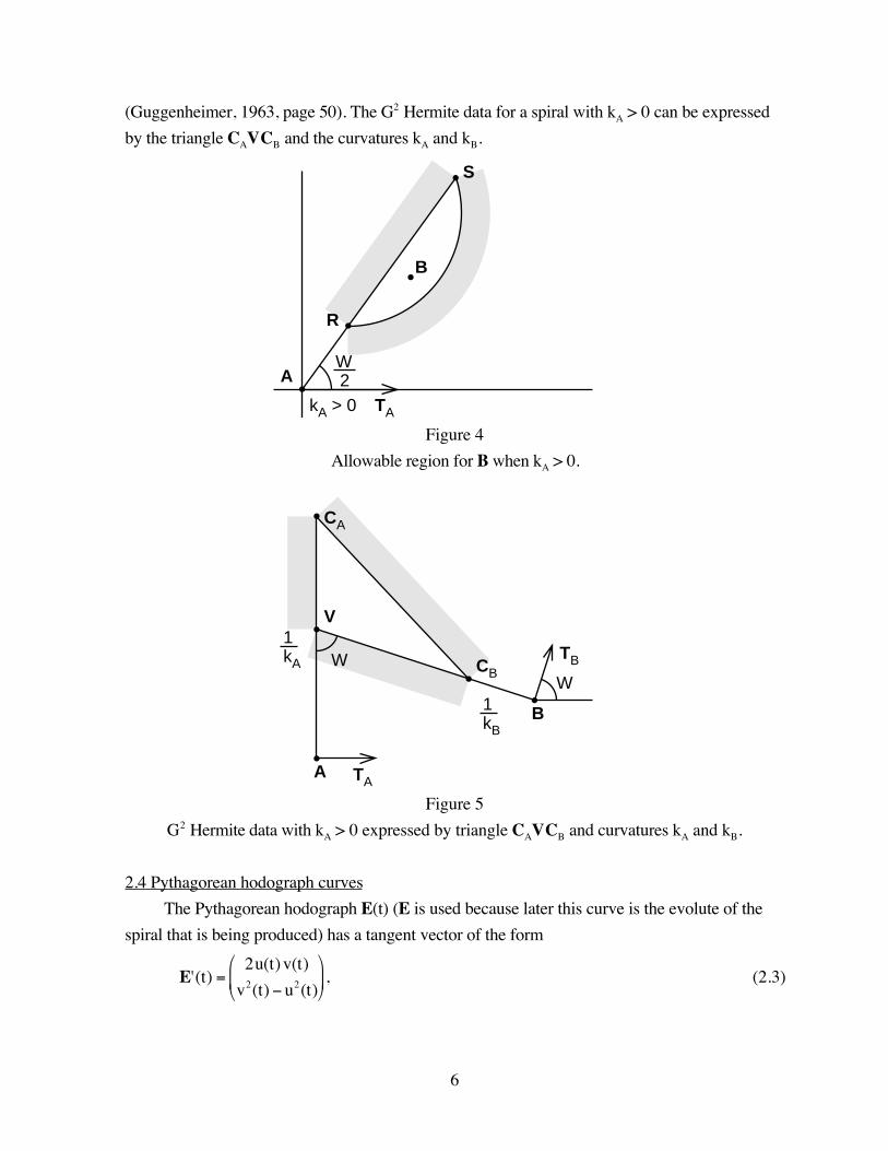
2.4 Pythagorean hodograph curves
The Pythagorean hodograph E(t) (E is used because later this curve is the evolute of the
spiral that is being produced) has a tangent vector of the form
E'(t) =2u(t)v(t)
v2(t) u2(t)
, (2.3)
Page 7
7
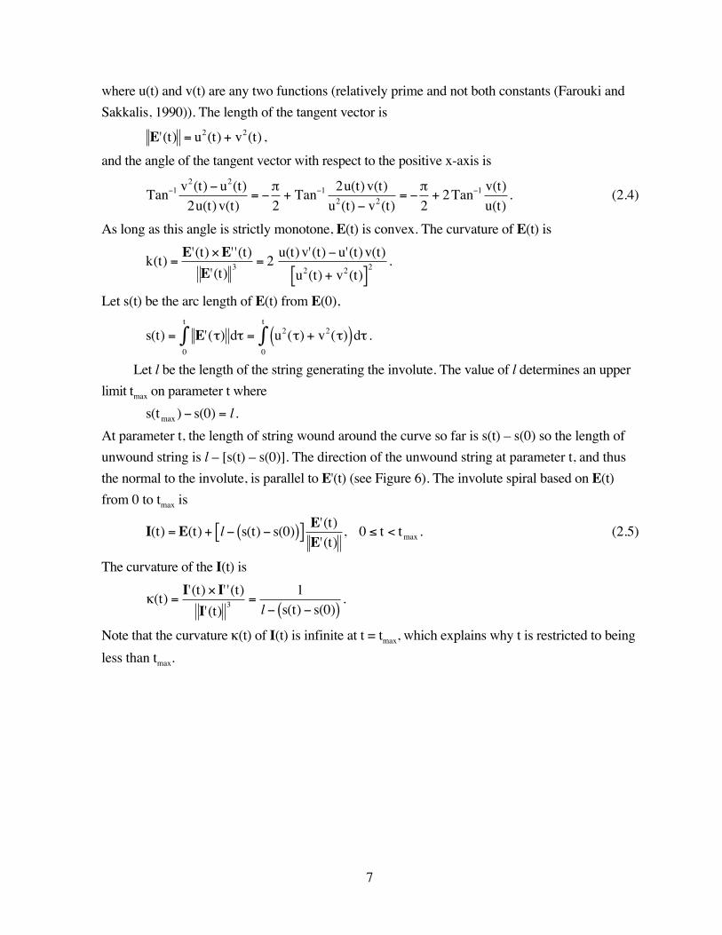
where u(t) and v(t) are any two functions (relatively prime and not both constants (Farouki and
Sakkalis, 1990)). The length of the tangent vector is
E'(t) = u2(t) + v2(t) ,
and the angle of the tangent vector with respect to the positive x-axis is
Tan 1 v2(t) u2(t)
2u(t) v(t)=
2+ Tan 1 2u(t)v(t)
u2(t) v2(t)=
2+ 2Tan 1 v(t)
u(t). (2.4)
As long as this angle is strictly monotone, E(t) is convex. The curvature of E(t) is
k(t) =E'(t) E' '(t)
E'(t)3 = 2
u(t)v'(t) u'(t) v(t)
u2(t) + v2(t)[ ]2 .
Let s(t) be the arc length of E(t) from E(0),
s(t) = E'( ) d0
t
= u2( ) + v2( )( )d0
t
.
Let l be the length of the string generating the involute. The value of l determines an upper
limit tmax on parameter t where
s(tmax ) s(0) = l .
At parameter t, the length of string wound around the curve so far is s(t) – s(0) so the length of
unwound string is l – [s(t) – s(0)]. The direction of the unwound string at parameter t, and thus
the normal to the involute, is parallel to E'(t) (see Figure 6). The involute spiral based on E(t)
from 0 to tmax is
I(t) = E(t) + l s(t) s(0)( )[ ]E'(t)E'(t)
, 0 t < tmax . (2.5)
The curvature of the I(t) is
(t) =I'(t) I' '(t)
I'(t)3 =
1
l s(t) s(0)( ).
Note that the curvature (t) of I(t) is infinite at t = tmax, which explains why t is restricted to being
less than tmax.
Page 8
8
E(0)
E(tmax)
E(t)
s(t) – s(0)
l – [s(t) – s(0)]
E'(t)I(t)
Figure 6
Involute of a convex curve.
In this paper, the functions u(t) and v(t) are chosen as simple rational functions so that E(t)
is a rational Pythagorean hodograph (Section 3) or as linear so that E(t) is a T-cubic (Section 4).
3. Finding the spiral that matches given G2 Hermite data, kA = 0
The spiral is generated as the involute of a rational Pythagorean hodograph curve that fits
inside the degenerate triangle VCB.
If u(t) and v(t) in (2.3) are chosen as
u(t) =u0t
+ u1 t , v(t) =v0t
+ v1 t ,
then E'(t) can be written in the form
E'(t) =1
t2P + 2Q + t 2R, 0 t 1, (3.1)
where
P =2u0 v0v0
2 u02
, Q =
u0 v1 + u1 v0v0 v1 u0 u1
, R =
2u1 v1v12 u1
2
. (3.2)
The angle from P to Q equals the angle from Q to R, call it , and the lengths ||P||, ||Q||, and
||R|| form a geometric progression. Let be a (positive) number for which
P =1Q , R = Q . (3.3)
Although P, Q, and R can be expressed in terms of the unknowns and ||Q||, it is convenient to
retain them in the expressions below. The following dot and cross products appear frequently:
Page 9
9
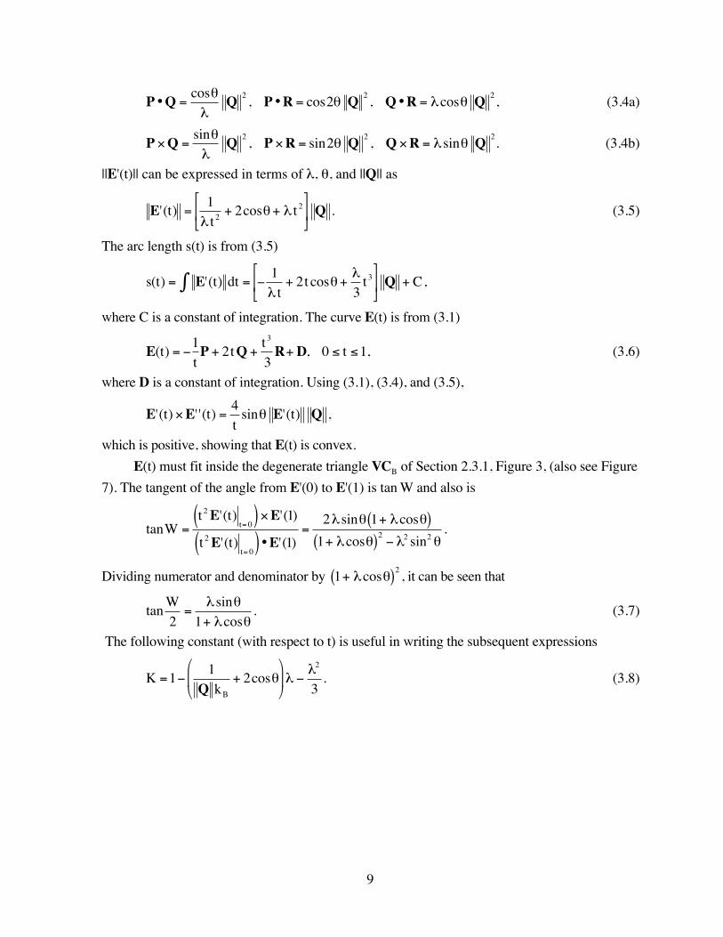
P •Q =cos
Q2, P •R = cos2 Q
2, Q •R = cos Q
2, (3.4a)
P Q =sin
Q2, P R = sin2 Q
2, Q R = sin Q
2. (3.4b)
||E'(t)|| can be expressed in terms of , , and ||Q|| as
E'(t) =1
t2+ 2cos + t 2
Q . (3.5)
The arc length s(t) is from (3.5)
s(t) = E'(t) dt =1
t+ 2t cos +
3t3
Q + C ,
where C is a constant of integration. The curve E(t) is from (3.1)
E(t) =1
tP + 2tQ +
t 3
3R+D, 0 t 1, (3.6)
where D is a constant of integration. Using (3.1), (3.4), and (3.5),
E'(t) E' '(t) =4
tsin E'(t) Q ,
which is positive, showing that E(t) is convex.
E(t) must fit inside the degenerate triangle VCB of Section 2.3.1, Figure 3, (also see Figure
7). The tangent of the angle from E'(0) to E'(1) is tan W and also is
tanW =t 2E'(t)
t= 0( ) E'(1)
t 2E'(t)t= 0( ) •E'(1)
=2 sin 1+ cos( )
1+ cos( )2 2 sin2
.
Dividing numerator and denominator by 1+ cos( )2, it can be seen that
tanW
2=
sin
1+ cos. (3.7)
The following constant (with respect to t) is useful in writing the subsequent expressions
K =11
Q kB+ 2cos
2
3. (3.8)
Page 10
10
A = I(0)
kA = 0
TA
W
W
B = I(1)
TB
1kB
CB = E(1)
V
E(t)
I(t)
Figure 7
E(t) for kA = 0 case.
Imagine unwinding a string along the curve E(t) from E(1) to form the involute I(t). The
length of unwound string at E(1) is 1
kB; the length of unwound string at E(t) is
1
kB+ s(1) s(t) =
1
tK 2 cos( ) t
2
3t 3
Q
. (3.9)
The involute spiral based on E(t) is
I(t) = E(t) +1
kB+ s(1) s(t)
E'(t)E'(t)
, (3.10)
and the curvature of I(t) is
(t) =1
1kB
+ s(1) s(t).
It is clear from (3.9) that this curvature approaches 0 as t approaches 0. Using (3.1), (3.5), (3.6),
and (3.9) in (3.10), it can be seen that the inverse powers of t in (3.6) and (3.9) cancel so that
I(0) = KP +D . (3.11)
The requirement that I(0) = A means
D =A +KP. (3.12)
Finally in matching the degenerate triangle VCB, E(1) – I(0) must be CB – A, so from (3.6) and
(3.11),
Page 11
11
E(1) I(0) = (K 1)P + 2Q +1
3R =CB. (3.13)
E'(0) points in the same direction as P from (3.1) and must point in the same direction as
R(– /2) TA. Taking the dot and cross products of (3.13) with QP , and using (3.7) and the
value of K in (3.8),
2 Q sin
3sin = CB,y
1
kB, (3.14)
2 Q sin
33+ cos( ) = CB,x . (3.15)
Equations (3.7), (3.14), and (3.15) are three equations for the three unknowns , , and ||Q||.
The ratio of (3.14) to (3.15) gives
sin
3+ cos=
CB,y
1
kBCB,x
= tan , (3.16)
where, referring to Figure 2, is the angle from TA to RB. The restrictions on B are equivalent
to 0 < < W/2. Equations (3.7) and (3.16) form a non-singular system of two linear equations
in the unknowns sin and cos with solution
sin =
2 tan tanW
2
tanW2
tan, cos =
3 tan tanW
2
tanW2
tan.
Knowing sin and cos means and can be found. This is a conversion from Cartesian
coordinates to polar coordinates, so without loss of generality, can be taken as positive. In the
present application, is not actually needed, cos and sin are sufficient. ||Q|| can be found
using either equation (3.14) or (3.15). With P pointing is the same direction as R(– /2) TA
(mentioned above), ||P|| given in (3.3), D defined in (3.12), E(t) defined in (3.6), I(t) in (3.10) is
determined. I(t) is a spiral that matches the G2 Hermite data in the zero curvature case.
The formula for I(t) in terms of , , and ||Q||, using P, Q, and R for convenience, is
I(t) =A +t
3
12cos + 6Kcos( ) t 4 t 2 + 3K t3
1+ 2 cos( ) t 2 + 2 t 4P
+2t
3
6 3Kt + 2 2 t 4
1+ 2 cos( ) t 2 + 2 t 4Q
+t 3
3
4 3Kt 4 cos( ) t 2
1+ 2 cos( ) t 2 + 2 t 4R ,
Page 12
12
where K is defined in (3.8).
4. Finding the spiral that matches given G2 Hermite data, kA > 0
The spiral is generated as the involute of a convex curve of length L (see equation (2.1))
that joins CA to CB and that fits inside triangle CAVCB. Since the convex curve is the T-cubic,
this involute is the class 3 curve treated in (Haddou, 1995) and (Pottmann, 1995a). There is a
unique T-cubic that fits inside triangle CAVCB, hereafter called the default T-cubic. The default
T-cubic does not depend on kA and kB. If the arc length of the default T-cubic is not equal to L,
the T-cubic will be modified to give a suitable convex curve of length L. The matching of the arc
length gives rise to three cases.
Papers by Roulier (1993, 1996) include theorems about how the length of a Bézier curve
changes with changes in the control polyline. They cannot be applied directly to this work
because here it is important to preserve the Pythagorean hodograph property.
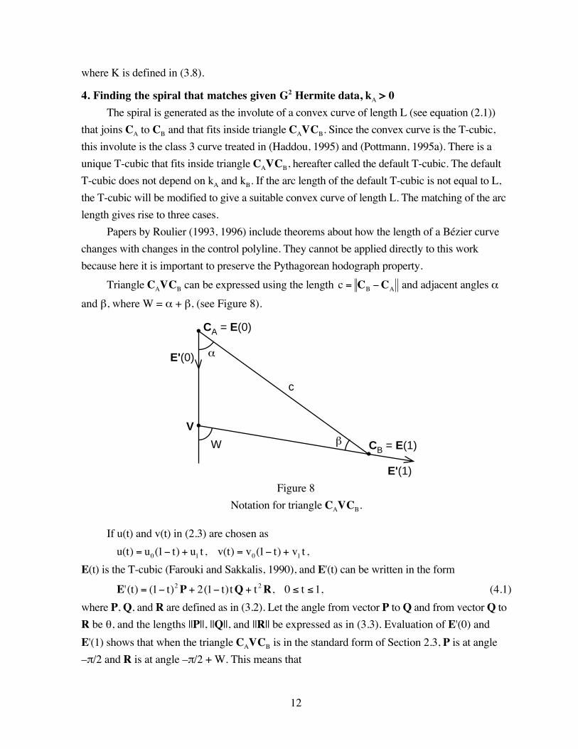
Triangle CAVCB can be expressed using the length c = CB CA and adjacent angles
and , where W = + , (see Figure 8).
W
α
β
CA = E(0)
CB = E(1)
V
E'(0)
E'(1)
c
Figure 8
Notation for triangle CAVCB.
If u(t) and v(t) in (2.3) are chosen as
u(t) = u0(1 t) + u1 t , v(t) = v0(1 t) + v1 t ,
E(t) is the T-cubic (Farouki and Sakkalis, 1990), and E'(t) can be written in the form
E'(t) = (1 t)2P + 2(1 t)tQ + t 2R, 0 t 1, (4.1)
where P, Q, and R are defined as in (3.2). Let the angle from vector P to Q and from vector Q to
R be , and the lengths ||P||, ||Q||, and ||R|| be expressed as in (3.3). Evaluation of E'(0) and
E'(1) shows that when the triangle CAVCB is in the standard form of Section 2.3, P is at angle
– /2 and R is at angle – /2 + W. This means that
Page 13
13
=W
2=
+
2. (4.2)
Although is now known in terms of and , it is convenient to retain in most of the
expressions below. Using (3.4), ||E'(t)|| can be expressed in terms of , , and ||Q||,
E'(t) =(1 t)2
+ 2(1 t)t cos + t 2
Q . (4.5)
The arc length s(t) is from (4.5)
s(t) = E'( ) d0
t
=t 3 3t 2 + 3t
+ ( 2t 3 + 3t2)cos + t 3
Q
3. (4.6)
The arc length of the default T-cubic from CA to CB is
LT = s(1) s(0) =1
+ cos +
Q
3, (4.7)
where, referring to (2.2),
c = CB CA < LT < V CA + CB V . (4.8)
The curve E(t) is
E(t) =1
3(t 3 3t 2 + 3t)P + ( 2t 3 + 3t2)Q + t 3R[ ] +CA, 0 t 1. (4.9)
The involute I(t) of E(t), calculated using (4.5), (4.6), and (4.9) in (2.5), appears to be quintic
divided by a quadratic, but on closer examination, it is seen to be a quartic over a quadratic (as
shown in (Pottmann, 1995a)).
E(t) is to be used as the convex evolute curve that fits inside triangle CAVCB, Figure 8;
hence E(0) = CA and E(1) = CB. Using (4.1) to (4.5) and (3.4),
E'(t) E' '(t) = 2sin E'(t) Q ,
which is positive, showing that E(t) is convex. and ||Q|| will now be found using triangle
CAVCB. From (4.9),
E(1) E(0) =1
3P +Q +R[ ]. (4.10)
The angles and give equations
sin =E'(0) E(1) E(0)( )
P c=
sin
3c
1+ 2cos
Q , (4.11a)
sin =E(1) E(0)( ) E'(1)
c R=sin
3c2cos +( ) Q . (4.11b)
The quotient of the above two equations and use of (4.2) gives a quadratic equation for ,
Page 14
14
sin+ sin
2
sin = 0. (4.12)
Equation (4.12) has one positive root. Once is known, equation (4.11a) gives
Q =3sin
sin
1
1+ 2 cosc . (4.13)
The length of the default T-cubic is from (4.7) and (4.13)
LT =sin
sin
1+ cos +
1+ 2 cosc . (4.14)
When triangle CAVCB is isosceles, = = , the formulas are especially simple:
=1, Q =3c
1+ 2cos, LT =
2 + cos
1+ 2cosc. (4.15)
The above analysis finds the default T-cubic that lies in triangle CAVCB, but the evolute
curve must also have the required length. There are three cases:
4.1 Case a: LT = L
In this case, the default T-cubic has the required length. The involute of the default T-cubic
produces a spiral that matches the given G2 Hermite data. Construct the spiral in (2.5) as the
involute of the default T-cubic E(t) in (4.9) with l = 1
kA (so that the initial curvature is kA) and
parameter range 0 t 1.
4.2 Case b: LT > L
In this case the default T-cubic is too long and a shorter convex curve that fits inside
triangle CAVCB is required. One method to shorten the evolute curve is to find a flatter T-cubic
by allowing the directions of the tangent vectors at the end points to move towards the direction
of CB – CA. The resulting spiral will have circular arcs joining at both ends.
Page 15
15
W
α
β
2α
CA = E(0)
CB = E(1)
c
V
VL
Vi
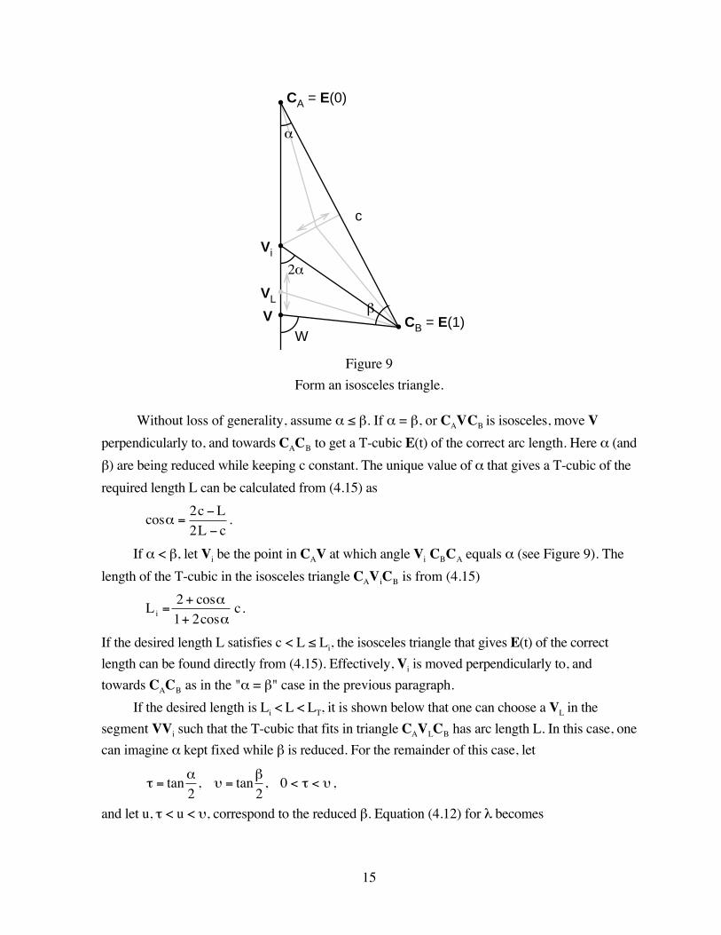
Figure 9
Form an isosceles triangle.
Without loss of generality, assume . If = , or CAVCB is isosceles, move V
perpendicularly to, and towards CACB to get a T-cubic E(t) of the correct arc length. Here (and
) are being reduced while keeping c constant. The unique value of that gives a T-cubic of the
required length L can be calculated from (4.15) as
cos =2c L
2L c.
If < , let Vi be the point in CAV at which angle Vi CBCA equals (see Figure 9). The
length of the T-cubic in the isosceles triangle CAViCB is from (4.15)
Li =2 + cos
1+ 2cosc .
If the desired length L satisfies c < L Li, the isosceles triangle that gives E(t) of the correct
length can be found directly from (4.15). Effectively, Vi is moved perpendicularly to, and
towards CACB as in the " = " case in the previous paragraph.
If the desired length is Li < L < LT, it is shown below that one can choose a VL in the
segment VVi such that the T-cubic that fits in triangle CAVLCB has arc length L. In this case, one
can imagine kept fixed while is reduced. For the remainder of this case, let
= tan2, = tan
2, 0 < < ,
and let u, < u < , correspond to the reduced . Equation (4.12) for becomes
Page 16
16
2
1+2
1+
u
1+2 1+ u2
2u
1+ u2= 0 . (4.16)
Replacing by , where
=1+
2
1+ u2, (4.17)
equation (4.16) becomes,
2+ u 2u = 0 ,
and its positive root is
=u +
2+14 u + u2
4u. (4.18)
Using (4.17), (4.18), the formulas
sin =2
1+2 , sin =
+ u
1+2 1+ u2
, cos =1 u
1+2 1+ u2
,
and replacing LT by L, equation (4.14) for u becomes
L =(1 u)( + u) + (1+ u) 2
+14 u + u2
(1+ u)( + u) + (1 u) 2+14 u + u2
c . (4.19)
Since and u are nonzero, the surd in (4.19) can be cleared to give a quadratic in u; namely,
(r +1) 3(r +1) 2 (r 1)[ ]u2 8 r2 1[ ] u + (r 1) (r +1) 2 + 3(r 1)[ ] = 0,
where r = L/c > 1. Because Li < L < LT, there is one root in ( , ). Notice the discriminant
12(r2 1) (r +1) 2 + (r 1)[ ]2 is almost a perfect square.
4.3 Case c: LT < L
In this case the default T-cubic is too short and a longer convex curve that fits inside
triangle CAVCB is required. One method to lengthen the evolute curve is to cut out an interior
part of the default T-cubic and scale both remaining parts so that they meet. This procedure
keeps the convex curve inside the triangle CAVCB, makes it longer, and gives it a cusp. The
resulting spiral will have a circular arc in its interior.
Page 17
17
CA = E(0)
CB = E(1)
E(t)
E(t)
E(e)
E(1 – e)
V
W
Figure 10
Cut out the interior of E(t).
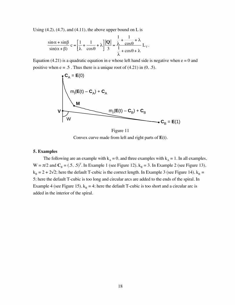
The left part of E(t) has parameter t = 0 to t = e; the right part of E(t) has parameter t = 1
– e to t = 1, where 0 < e < .5 (see Figure 10). Now scale the left part by ml > 1 (about CA) and
the right part by mr > 1 (about CB) so that the two parts meet at M forming a cusp (see Figure
11). Scaling does not change the direction of a tangent vector, so the curve that is produced is a
convex curve with a cusp. Two expressions for M give a vector equation for ml and mr,
M =ml E(e) CA( ) +CA =mr E(1 e) CB( ) +CB ,
from which
ml =CB CA( ) E(1 e) CB( )E(e) CA( ) E(1 e) CB( )
, mr =E(e) CA( ) CB CA( )
E(e) CA( ) E(1 e) CB( ).
The arc length of this convex curve with a cusp must satisfy
ml s(e) s(0)[ ] +mr s(1) s(1 e)[ ] = L . (4.20)
Expressions to help rewrite equation (4.20) are given in the Appendix. Equation (A.1) using
(4.7) to eliminate ||Q|| becomes
L
LT
1
1+ cos +
6sin2=
2e2 3e +1
2e2 + 3e( )1
+
+ 2 2e2 3e + 3( )cos
.
The above equation can be rearranged to
L
LT
1
1+ cos +
6sin2
2e2 + 3e( )1
+
+ 2 2e2 3e + 3( )cos
2e2 3e +1[ ] = 0 . (4.21)
In Case c, L satisfies
LT < L < V CA + CB V =sin + sin
sin( + )c .
Page 18
18
Using (4.2), (4.7), and (4.11), the above upper bound on L is
sin + sin
sin( + )c =
1+
1
cos+
Q
3=
1+
1
cos+
1+ cos +
LT .
Equation (4.21) is a quadratic equation in e whose left hand side is negative when e = 0 and
positive when e = .5 . Thus there is a unique root of (4.21) in (0, .5).
CA = E(0)
CB = E(1)
ml(E(t) – CA) + CA
mr(E(t) – CB) + CB
M
V
W
Figure 11
Convex curve made from left and right parts of E(t).
5. Examples
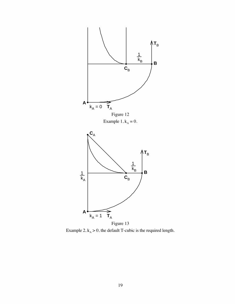
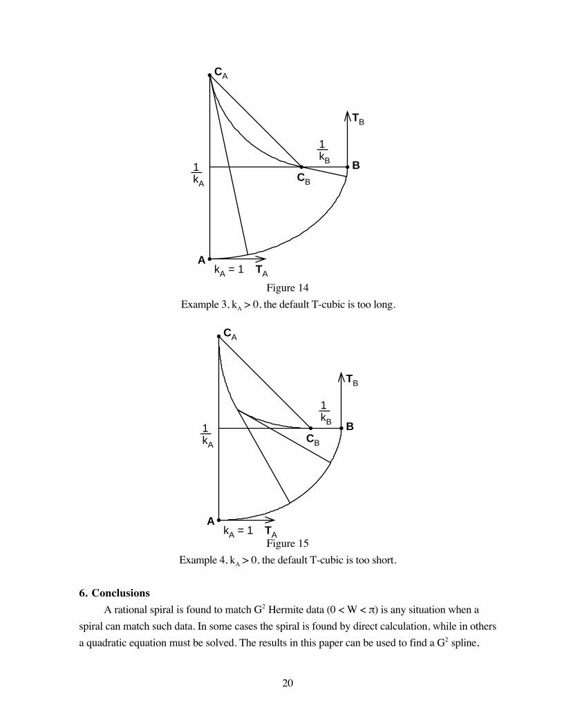
The following are an example with kA = 0, and three examples with kA = 1. In all examples,
W = /2 and CB = (.5, .5)T. In Example 1 (see Figure 12), kB = 3. In Example 2 (see Figure 13),
kB = 2 + 2 2; here the default T-cubic is the correct length. In Example 3 (see Figure 14), kB =
5; here the default T-cubic is too long and circular arcs are added to the ends of the spiral. In
Example 4 (see Figure 15), kB = 4; here the default T-cubic is too short and a circular arc is
added in the interior of the spiral.
Page 19
19
AkA = 0
BCB
1kB
TA
TB
Figure 12
Example 1, kA = 0.
AkA = 1
B
CA
CB
1kA
1kB
TA
TB
Figure 13
Example 2, kA > 0, the default T-cubic is the required length.
Page 20
20
AkA = 1
B
CA
CB
1kA
1kB
TA
TB
Figure 14
Example 3, kA > 0, the default T-cubic is too long.
AkA = 1
B
CA
CB
1kA
1kB
TA
TB
Figure 15
Example 4, kA > 0, the default T-cubic is too short.
6. Conclusions
A rational spiral is found to match G2 Hermite data (0 < W < ) is any situation when a
spiral can match such data. In some cases the spiral is found by direct calculation, while in others
a quadratic equation must be solved. The results in this paper can be used to find a G2 spline,
Page 21
21
each segment of which is a spiral, that matches a sequence of G2 Hermite data when such a curve
is possible.
Acknowledgements
The authors acknowledge the financial support of the Natural Sciences and Engineering
Research Council of Canada for this research. The second author appreciates the hospitality of
the University of Dundee, Dundee, Scotland, and the third author appreciates the hospitality of
the Institute for Biodiagnostics, Winnipeg, Canada. We thank two anonymous referees for
pointing out the references of Pottmann and of Haddou to previous work in this area.
References
Farin, G.E., 1997. Curves and Surfaces for Computer-Aided Geometric Design: A Practical
Guide, Fourth Edition. Academic Press, San Diego.
Farouki, R.T., Sakkalis, T., 1990. Pythagorean hodographs. IBM Journal for Research and
Development 34, 736-752.
Guggenheimer, H.W., 1963. Differential Geometry. McGraw-Hill, Inc., New York.
Haddou, R. A., Biard, L., 1995. G2 Approximation of an offset curve by Tschirnhausen quartics,
in: Daehlen, M., Lyche, T., Schumaker, L. L., (Eds.), Mathematical Methods for Curves
and Surfaces, Vanderbilt University Press, pp.1-10.
Kuroda, M., Mukai, S., 2000. Interpolating involute curves, in: Cohen, A., Rabut, C., Schumaker,
L. L. (Eds.), Curve and Surface Fitting: Saint Malo 1999, Vanderbilt University Press,
Nashville, pp. 1 - 8.
Meek, D.S., Walton, D.J., 1992. Clothoid spline transition spirals. Mathematics of Computation
59, 117-133.
Meek, D.S., Walton, D.J., 1998. Planar spirals that match G2 Hermite data. Computer Aided
Geometric Design 15, 103-126.
Pottmann, H., 1995a. Rational curves and surfaces with rational offsets. Computer Aided
Geometric Design 12, 175-192.
Pottmann, H., 1995b. Curve design with rational Pythagorean-hodograph curves. Advances in
Computational Mathematics 3, 147-170.
Press, W.H., Teukolsky, S.A., Vetterling, W.T., Flannery, B.P., 1992. Numerical Recipes in C,
second ed. Cambridge University Press, Cambridge, England.
Roulier, J.A., 1993. Specifying the arc length of Bézier curves. Computer Aided Geometric
Design 10, 25-56.
Roulier, J.A., Piper, B., 1996. Prescribing the length of parametric curves. Computer Aided
Geometric Design 13, 3-22.
Page 22
22
Appendix - formulas for Section 4.3, Case c
Some formulas based on (4.6), (4.9), and (4.10),
E(e) CA =e
3e2 3e + 3( )P + 2e2 + 3e( )Q + e2R{ },
E(1 e) CB =e
3e2P + 2e2 + 3e( )Q + e2 3e + 3( )R{ },
E(e) CA( ) E(1 e) CB( )
= sin(1 e)e2
3
2e2 3e2 2e2 3e + 3( )cos + 2e2 3e( )
Q
2,
CB CA( ) E(1 e) CB( ) = sin(1 e)e
3
e+ 2cos + (1 e)
Q
2,
E(e) CA( ) CB CA( ) =sin(1 e)e
3
1 e+ 2cos + e
Q
2,
s(e) s(0) =e
3
e2 3e + 3+ 2e2 + 3e( )cos + e2
Q ,
s(1) s(1 e) =e
3
e2+ 2e2 + 3e( )cos + e2 3e + 3( )
Q ,
ml =1
e
e+ 2cos + (1 e)
2e2 3e( )1
+
2 2e2 3e + 3( )cos
,
mr =1
e
1 e+ 2cos + e
2e2 3e( )1
+
2 2e2 3e + 3( )cos
,
L =
2e2+ 3e( )1
+
2
+ 2e2 3e + 6( )1
+
cos + 6 2e2 3e +1( ) + 4 2e2+ 3e( )cos2
2e2+ 3e( )1
+
+ 2 2e2 3e + 3( )cos
Q
3
=1
+ cos + +6 2e2 3e +1( )sin2
2e2+ 3e( )1
+
+ 2 2e2 3e + 3( )cos
Q
3. (A.1)


![involute profile - [email protected]](https://static.documents.pub/doc/80x56/62038846da24ad121e4a82be/involute-profile-emailprotected.jpg)

