1

An Iterative Approach to Estimation with Multiple High-Dimensional Fixed Effects

Siyi Luo, Wenjia Zhu, Randall P. Ellis

March 23, 2017

Department of Economics, Boston University

Abstract

Controlling for multiple high-dimensional fixed effects while estimating the effects of specific policy or treatment variables is common in linear models of health care utilization. Traditional estimation approaches are often infeasible with multiple very high dimension fixed effects. Additional challenges arise if sample sizes are large, data are unbalanced, and when instrumental variables and clustered standard error corrections are also needed. We develop a new estimation algorithm, implemented in SAS, that accommodates all of these practical estimation challenges.

In contrast with most existing algorithms that absorb multiple fixed effects simultaneously, our algorithm sequentially absorbs fixed effects and repeats iterating until fixed effects are asymptotically eliminated. Written in SAS, the main advantage of our approach is that it is easy to use and able to accommodate extremely large datasets without requiring that data be actively stored in memory. The main disadvantage is that our algorithm does not generate parameter estimates of each fixed effect, but only of the parameters of interest.

Monte Carlo simulations confirm that our approach exactly matches Stata’s reghdfe estimation results in all the models, which is itself identical to estimating linear models with fixed effect dummies. We then apply our algorithm to extend Ellis and Zhu (2016) using US employer-based health insurance market data. From a sample of 63 million individual-months we remove fixed effects for 1.4 million individuals, 150,000 distinct primary care physicians (PCPs), 3,000 counties, 465 employer-year-single/family and 47 monthly dummies, and find that narrow network plans (exclusive provider organizations, health maintenance organizations and point-of-service plans) reduce the probabilities of monthly provider contacts (by 11.1%, 5.7%, 3.6%, respectively) relative to preferred provider organization plans (PPOs), while consumer-driven/high-deductible plans are statistically insignificantly different (95% CI: -3.6% to 4.6%).

Keywords: multiple high-dimensional fixed effects, big data, iterative algorithm, Monte Carlo simulations, health care utilization

JEL codes: I11, G22, I13

Acknowledgements: We are grateful to Iván Fernández-Val, Coady Wing, and participants at 2016 Biennial Conference of the American Society of Health Economists, 2015 Annual Health Econometrics Workshop, Boston University Econometrics Reading Group and Boston University Empirical Microeconomics Reading Group for useful comments and insights. All remaining errors belong to the authors.

2

1. Introduction

The simplest way to estimate a two-way fixed effect model is to include fixed effects as dummy variables and obtain the least squares dummy variable (LSDV) estimator. When the numbers of levels for both fixed effects are small, using the LSDV model makes sense and is straightforward. When only one of the fixed effects has a large number of levels (i.e., the fixed effect is high dimensional), it is often feasible to include the other fixed effect as dummies. This leaves one high-dimensional fixed effect to absorb and we can apply the usual method of one-way fixed effect models. In both cases, the LSDV approach will work well regardless of whether data are balanced or not.

The LSDV method, however, can become computationally infeasible as sample sizes and the numbers of high-dimensional fixed effects increase, necessitating the absorption of two or more high-dimensional fixed effects. Although SAS has the capability of handling large sample size estimation, there are challenges in the practical implementation. For example, SAS’s built-in program for estimating OLS fixed effects models is limited in the number of fixed effects levels that it can include in the model due to memory constraint and the ability to internally index variable levels.1

One alternative is to estimate a transformed version of the model in which fixed effects are eliminated. One commonly used method is Within transformation. Note that there can be multiple ways of Within transforming the model, but the one that gives the same parameter estimates as LSDV is the optimal transformation (Balázsi, Mátyás, and Wansbeek 2015). But Balázsi, Mátyás, and Wansbeek (2015) show that in a simple model with two fixed effects and balanced data, the Within transformation has a 1 Two commonly used SAS procedures for fixed effects are PROC GLM and PROC HPMIXED. Sample code for PROC GLM is: PROC GLM DATA=TEST; ABSORB FE1;

CLASS FE2; MODEL Y = X FE2 / SOLUTION;

RUN; Although one high dimensional FE1 can be absorbed, except in special cases a second cannot. Attempting to estimate FE2 as a high dimensional fixed effect results in the following error message: ERROR: Number of levels for some effects > 32767. For more information about this error, see SAS’s online documentation http://support.sas.com/documentation/cdl/en/statug/63033/HTML/default/viewer.htm#statug_glm_sect039.htm/. Sample code for PROC HPMIXED is: PROC HPMIXED DATA=TEST;

CLASS FE1 FE2; MODEL Y = X FE1 FE2 / SOLUTION;

RUN; Note that PROC HPMIXED does not allow ABOSORB statement for including fixed effects. For a model of over 100 million observations and two fixed effects of about 3000 and 2 million levels respectively, running the above codes gives the following error message. ERROR: The HPMIXED procedure stopped because of the insufficient memory.

3

straightforward formula. For models with more than two fixed effects and under common data issues such as unbalanced data, transformation can become intractable.2

In this paper, we propose an alternative approach to transform models featuring large sample sizes and high-dimensional fixed effects. As opposed to the Within transformation which absorbs fixed effects in one step, our proposed method demeans variables with respect to each one of the fixed effects sequentially and clears up fixed effects by iterations. One advantage of our method is that it is easy to implement. Also, this method can be generalized to more complicated models such as those containing more than two high-dimensional fixed effects and instrumental variables without increasing the complexity of the algorithm. Finally, we implement this method in SAS that is particularly capable of handling large data sets. A disadvantage of our approach is that we do not recover the estimated fixed effects, but only of the policy variables of interest.

Our approach is motivated by the Guimaraes and Portugal (2010) algorithm, labeled the GP algorithm that is commonly used to deal with multiple high-dimensional fixed effects. This algorithm is attractive because it uses the iteration and convergence implementation of Least Squared estimation instead of the explicit calculation of the inverse of matrices. Another valuable innovation is that it stores and retrieves each fixed effect as a column vector, which compresses the dimensions of fixed effects to ones. Hence in each iteration, the estimation of each fixed effect merely involves taking simple average of residuals by groups, after which the OLS regression is then run for other regressors along with the updated fixed effect vector as a variable. After convergence of the estimates, the fixed effects remain identifiable.

An efficient GP algorithm has been programmed as a user build-in function in Stata written by Sergio Correia (2015)3 called reghdfe, which we use as a benchmark for this paper. The Correia (2015) algorithm represents a significant enhancement in the GP algorithm in that it is designed to converge more quickly, is flexible about the number of fixed effects, allows for interactions between fixed effects as well as interactions between fixed effects and other categorical variables, and is integrated with IV/2SLS regression.4

2 In terms of implementation, although SAS builds in a convenient program, PROC GLM, to absorb high-dimensional fixed effects, the current version of the program does not allow absorption of multiple fixed effects that would provide the equivalent results of the LSDV estimator. For example, the following procedure estimates the model Y = X + FE1*FE2 + error, which is not equivalent to the model of interest Y = X + FE1 + FE2 + error. PROC GLM DATA=TEST;

ABSORB FE1 FE2; MODEL: Y = X / SOLUTION;

RUN; 3 Sergio Correia built and released a Stata user written package reghdfe in July 2014, and has continually updated it. The last update was on June 19th, 2015. 4 An example of using this command is:

4

The reghdfe also allows cluster-robust variance estimation (CRVE) (Cameron and Miller 2015), which is a nontrivial enhancement.

As shown in Table 1, in terms of functionality, Stata’s reghdfe combines ivregress that allows clustered standard error correction and instruments, and a2reg that accommodates two or more high-dimensional fixed effects. While easy to use and fast, reghdfe is unable to handle extremely large datasets since it relies upon retaining all working data in memory during execution and tends to fail due to a lack of memory on very large datasets on most computers.5 SAS is an attractive language for manipulating very large datasets, whether that be large sample sizes N, large numbers of parameters K or large numbers of fixed effects. While not as efficient as some other programming environments, SAS is an important and convenient environment since SAS is designed to process essentially infinite size datasets without attempting to retain the full dataset in memory while performing calculations.6

Like reghdfe, our ultimate goal is to develop an estimation algorithm that can be used to estimate linear regression models with two or more high-dimensional fixed effects, as well as 2SLS, and CRVE in very large samples. Even though SAS currently provides convenient programs for estimating models with large numbers of fixed effects (PROC GLM), performing 2SLS (PROC SYSLIN), or generating standard errors that correct for clustered errors (PROC SURVEYREG), it does not yet have procedures that allow for all three problems to be corrected simultaneously (Table 1). Moreover, convenient programs for fixed effects, 2SLS estimation, and the correction for clustered errors each involve creating very large temporary files that are a multiple of the size of the original datasets, and can often create storage problems during estimation. Our iterative algorithm (TSLSFECLUS), implemented in SAS, attempts to capture all these various features, and its computation and estimation performance is compared with that of reghdfe to justify the validity of our algorithm (Table 1).

The implementation of our algorithm involves three steps: (1) Absorb fixed effects sequentially from all dependent and explanatory (including instrumental) variables; (2) estimate the model using the standardized variables; (3) repeat and calculate the maximum absolute value of the percentage difference between adjacent iterations among parameters of interest, and report estimates when the percentage difference falls below a pre-specified threshold.

reghdfe outcome x (y=z), absorb (fe1=i.FE1 fe2=i.FE2) vce (cluster cluster) 5 Note that memory is needed by Stata and most packages not only for holding data, but also for workspace for manipulating matrices and storing interim results. 6 SAS was developed at a time when memory was expensive, but tapes could store essentially infinite length datasets. It still relies on sequential data processing more than most statistical packages, and hence can deal with very large N and K samples reasonably well.

5

We perform Monte Carlo simulations to evaluate the performance of our algorithm. A variety of datasets are considered with 95,000 to 100,000 observations and variations in the number of fixed effects, sample balance, correlations between fixed effects and control variables, extent of endogeneity, and interdependence between fixed effects. In some of the models, we feasibly allow standard error corrections to adjust for clustering, by applying the analytical formula described in Section 2.2.

The proposed algorithm is applied to US employer-based health insurance market data to examine how health plan types affect health care utilization. Our analysis sample contains about 63 million observations from which we remove fixed effects for 1.4 million individuals, 3,000 counties, 150,000 primary care doctors, 465 employer*year*single/family coverage, and 47 monthly time dummies to predict plan type effects on monthly health care utilization. By simultaneously controlling for individual, doctor, county, time, and employer*year*single/family fixed effects, our identification comes from consumers’ movement between health plan types. Our iterative algorithm not only controls for these multiple high-dimensional fixed effects, but also uses instrumental variables to control for endogenous plan choice and standard error corrections to adjust for clustering at the employer level. Our estimates show that the breadth of provider networks dominates cost sharing in influencing consumers’ decision to seek care.

The rest of the paper is organized as follows. Section 2 describes our iterative algorithm in a two-way fixed effect model framework, and proves a theorem that under two specific assumptions (Quasi-Balance and Strict Exogeneity), our algorithm converges to the simple least square model with true policy variable parameter values that is equivalent to the original specification with two types of fixed effects. In Section 3, we conduct Monte Carlo simulations to evaluate the validity of our algorithm. We then show in Section 4 that our algorithm is feasible to estimate a model of health care utilization on a real data set that requires controlling simultaneously for patients, providers and counties, each of high dimension. Finally, Section 5 concludes and discusses the next steps.

2. An Iterative Estimation Algorithm

2.1. Model Setup

In this section, we present our iterative algorithm for a simple linear two-way fixed effect model. We show (in progress) that under certain assumptions, remaining fixed effects are asymptotically eliminated, generating converged values which are unbiased and consistent estimates of the LSDV estimator of the parameter of interest.

Consider a two-way fixed effect model:

6

(1)

∈ ⊆ 1, 2, … ,

∈ ⊆ 1,2, … ,

Remark:

When ≡ ,∀ and ≡ , ∀ , the data is a balanced panel. Otherwise, there are missing observations and the panel is unbalanced. Without any loss in generality, assume that , so that the higher dimensionality fixed effect is always absorbed first.

The idea of our algorithm is to sequentially absorb fixed effects and repeats iterating until fixed effects are asymptotically eliminated. Specifically, we employ the following three-step procedure.

Step 1: Demean all dependent and independent variables by each one of the fixed effects sequentially, and estimate the demeaned model.

Step 2: Repeat Step 1 until fixed effects converge to a constant.

Step 3: Model parameters (coefficients and cluster-robust standard errors) are then estimated by least squares regression on the final demeaned model.

Using Model (1), our algorithm can be laid out as the following.

1st iteration:

1) Demean and over i

⋅ ⋅1

‖ ‖∈

⋅

≡ ∙1

‖ ‖∈

2) Demean the resulting and over t

⋅ ⋅1

‖ ‖1

‖ ‖∈∈

⋅

≡ ⋅1

‖ ‖∈

1‖ ‖

1‖ ‖

∈∈

7

where and are the remaining fixed effects after 1st iteration defined as:

≡1

‖ ‖1

‖ ‖∈∈

≡1

‖ ‖∈

Similarly, the regression model after (k+1)th iteration can be written as:

≡ ⋅

where

≡1

‖ ‖1

‖ ‖∈∈

≡1

‖ ‖∈

2

Assumption 1: Quasi-Balance

For any two time periods s and t, there exists an individual who is observed in both periods.

∀ , ∈ , , … , , ∃ . . ∈ ∈

Assumption 1 restricts the extent of unbalance of a dataset, although it is in fact a relatively loose condition which could be commonly observed in most of the datasets. This assumption is saying that for any pair of time periods, we can always observe at least one individual who appears in both periods. In other words, it rules out the type of dataset in which there are two periods where the pools of individuals are completely different. When Assumption 1 fails, for the two periods in which the whole individual sample pools are different, time fixed effects cannot be identified because individual fixed effects are nested within these two-period time fixed effects. The time fixed effects for these two periods would then be equivalent to the sum of individual fixed effects for the corresponding two sample pools.

Note that the way that Assumption 1 is stated depends on the order by which fixed effects are absorbed. In the current case, individual fixed effect is absorbed first and followed by time fixed effect, assuming that . If the order of absorption is reversed because

8

, then Assumption 1 would require that for any two individuals, there exists a time period that is observed for both individuals.

Theorem 1:

For model (1), if the dataset satisfies Assumption 1, then starting from any initial

value of ≡ , the remaining fixed effects converge to a constant vector, i.e.

→ ∀ , as → ∞.

For detailed proof, see Appendix A.

By Theorem 1, → ∀ and we can easily derive from equation (2) that →∀ . So the remaining individual and time fixed effects will be cancelled out with each

other upon convergence. In other words, by iterating the sequential absorption, fixed effects are eliminated asymptotically.

Theorem 2:

For model (1) under Assumption 1, the OLS/2SLS estimator from each iteration also converges, and converges to the LSDV estimator of .

For a detailed proof, see Appendix A.

Corollary 1:

If the OLS/2SLS estimator converges to the LSDV estimator, the remaining fixed effects converge to a constant vector.

For a detailed proof, see Appendix A.

Ideally, once the remaining fixed effects converge, we can then obtain an unbiased and consistent estimator. However, in practice, convergence of remaining fixed effects could not be observed explicitly. From corollary 1, we can instead check the convergence criterion on the estimates of the demeaned variables from each iteration

, , … , , … , ∞ . In practical implementation, we define convergence as when the largest absolute percentage change between two consecutive iterations among parameters of interest is below 10-4. For a detailed description of the implementation, see Appendix B.

9

Assumption 2: Strict Exogeneity

The idiosyncratic error is strictly exogenous.

1) :∀ , ∈ , , … , , , ∈, , … , , , , .

2) and instruments :∀ , ∈ , , … , , , ∈, , … , , , , .

Theorem 3: Under Assumption 2, the estimates from Step 3 are unbiased and consistent.

For a detailed proof, please see Appendix A.

The above algorithm applies to both models with and without endogeneity. With endogeneity, the same predictions are concluded for the 2SLS model, since 2SLS model could be rewritten equivalently as a reduced form where our algorithm applies.

2.2. Clustering Standard Errors

In many economic settings, standard errors are not necessarily independent but correlated within groups (e.g., schools, households, etc.), a phenomenon known as “clustered standard errors”. For example, student performance may be correlated within schools, and health spending is likely to be correlated within households. Suppose we allow errors to cluster at G level. Let g denote gth element in G. Following Cameron and Miller (2015), clustered errors can be expressed as:

| , 0 unless ′

Then the cluster-robust variance estimator (CRVE) can be written as:

where is a ∑ matrix of the demeaned s of the converged model,

∑ ∊ and ′ .

In the empirical estimation, we calculate cluster-robust standard errors by applying the above formula to the converged model where ( , are the demeaned values.

10

3. Monte Carlo Simulations

3.1. Pseudo Data Generating Process

We generate pseudo data sets according to model (1). In particular, we allow correlation between the fixed effects and the control variables x (see Moulton (1990) for a discussion of the importance of this type of correlation). We also allow the flexibility to include clustered errors that introduce correlation of errors within clusters.

Denote = number of individuals; = number of time periods; = correlation between control variable and individual fixed effects; = correlation between control variable and time fixed effects; = number of missing observations

We start by constructing a balanced panel, and then generate an unbalanced one by randomly dropping M observations. Details of data construction are as follows.

Step 1: Generate fixed effects, and from scaled uniform distribution, as follows: 1, 2, … , , ~10 ∗ 0,1

1, 2, … , , ~10 ∗ 0,1

Step 2: For each observation, generate error terms and from a bivariate normal distribution.

1, 2, … , , 1,2, … ,

, ~

For which we can simplify to a standard bivariate normal distribution:

, ~ 00

11

where is the correlation between and for 1, 2, … , , 1, 2, … , 7.

To operate this, we draw , pairs as the following:

1, 2, … , , 1, 2, … ,

~ 0,1 and ~ 0,1

1 8

7 Note that when variable is exogenous, equals 0.

11

To build in clustering of standard errors, we alternatively construct errors , as the

following assuming without loss of generality that errors are clustered within individuals over time:

1, 2, … ,

~ 0,1

, 0,1, 1, 2, … ,

where governs the serial correlation of errors within individuals and is fixed at 0.5 in all the simulations. Note that it is important that is not equal to 0 or 1, because otherwise there would be no variation in errors within individuals and would be completely absorbed in the same manner as the individual fixed effect , in which case no random errors would be left in the model.

For clustered standard errors, we focus on models without endogeneity only, i.e. 0. Then by construction,

, ~ 00

00 1

Step 3: Generate instrumental variable from a uniform distribution, as follows:

1, 2, … , , 1, 2, … , , ~10 ∗ 0,1

Step 4: Generate control variable that is potentially endogenous

1, 2, … , , 1, 2, … ,

∗ ∗ where the control variable is a linear combination of instruments, two fixed effects and an error term, with and indicating the correlation between control variable and each of the two fixed effects.

Step 5: Construct outcome variable according to the following process.

2 ∗

8 Proof: Note that 0, 1

1 1 , , , 1

, 1 , . These elements together constitute a bivariate normal

distribution.

12

Note that is endogenous if (and thus ) and are correlated. Otherwise, is exogenous. In both cases, we construct unbalanced data by randomly selecting M observations to drop from the balanced data.

3.2. Variations in Parameters

Our simulation model according to (1) defines 7 random variables , , , , , , and 6 parameters , , , , , . We estimate both OLS and 2SLS models with multiple fixed effects. We estimate each model using our iteration procedure and compare it with the LSDV estimate or equivalently estimate from the optimal Within transformation output by Stata.9

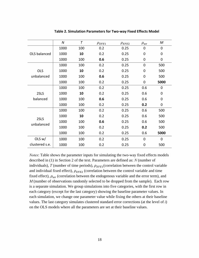
We conduct simulations by varying one parameter at a time while keeping other parameters fixed at the baseline values, as shown in Table 2. The baseline is , , , , , = {1000, 100, 0.2, 0.25, 0, 0} for OLS and , , , , , = {1000, 100, 0.2, 0.25, 0.6, 0} for 2SLS models. We explore

variations along (1) sample size (10, 100), (2) correlation between the control variable and fixed effects (0.2, 0.6), and (3) number of missing observations (0, 500, 5000). For 2SLS models, we additionally simulate the correlation between the endogenous variable and the error term, , at 0.6 and 0.2. Finally, we examine OLS models with and without clustered standard errors. In this ceteris paribus analysis, we test on the robustness of our algorithm and the relationship between each parameter and the convergence speed. The relevant discussion and investigation on improving our algorithm will be presented in our future work.

3.3. Results

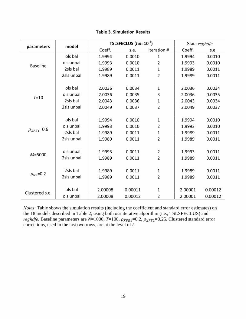
Table 3 shows the simulation results. Consistent with the analytical model, we find that for balanced data, convergence happens after the first iteration. The unbalanced model converges after the second or third iteration depending on the specific data structure. Furthermore, other things being equal, estimates using smaller samples are less precise as evident in bigger standard errors. In our specific data generating process, changing the correlation between control variable and fixed effects does not affect model estimation. Finally, the iterative results match well with the Stata default output, including standard errors that match with the Stata default outputs for all the variations of the model being examined here.

9 We use Stata’s built-in programs reghdfe to output results as our benchmark.

13

4. Empirical Example

4.1. Health Plan Type Effects on Health Care Utilization

We now illustrate the proposed method using US employer-sponsored health insurance market data to extend the analyses in Ellis and Zhu (2016).

We use data from the Truven Health Analytics MarketScan® Research Databases from 2007 to 2011 that contain detailed claims information for individuals insured by large employers in the US. The analysis sample contains 1.4 million individuals, ages 21-64, who are continuously insured from 2007 through 2011, with over 60 million treatment months for which we can assign an employer, a plan type, and a primary care physician (PCP). More details about construction of the analysis sample can be found in Ellis and Zhu (2016). The extension of their results in this paper is that we include 150,000 primary care physician (PCP) fixed effects in addition to the 1.4 million individual and 3,000 county fixed effects, so that plan effects control not only for individual and geographic variation, but also in the specific PCPs seen by each consumer.

We estimate the health plan type effects on the monthly utilization of health care (more specifically, the probability of seeking care in a month) using the following linear specification.

, (3)

where is the dependent variable for consumer i in month t. Five plan dummies, ,

are included one for each plan type {EPO, HMO, POS, COMP, CDHP/HDHP}. The omitted plan type is PPO, and hence the estimated coefficients give the plan type

effects as a difference from PPOs.10 We control for an enrollee’s health status11 , ,

enrollee fixed effects , primary care physician fixed effects , employee county fixed effects , and monthly time fixed effects . In addition, we include employer*year*family coverage fixed effects , in the regression to control for the fact that the underlying employer characteristics may make them more or less likely to offer each plan type.

To deal with endogeneity of plan type choice, we instrument observed individual plan type choice by the simulated probabilities of the plan type chosen by the individual’s household. We estimate household choice of health plans by applying a multinomial logit model separately for each employer*year*family coverage type combination, each

10 Plan type acronyms are: EPO (Exclusive Provider Organization), HMO (Health Maintenance Organization), POS (Point of Service, non-capitated), COMP (Comprehensive), and CDHP/HDHP (Consumer-Driven/High-deductible Health Plan), and PPO (Preferred Provider Organization). 11 We use prospective model risk score predicting total spending estimated from the prior twelve months of diagnoses to capture the patient’s overall health status.

14

controlling for the head-of-household age and gender, family size, whether a spouse is present, whether the household added a new baby in the previous twelve months, and the prospective model risk scores summed up for adults in the household predicting total spending. The predicted values tell us why individual i1 in one household is more or less likely than individual i2 in another household to be in plan type p at employer E in year Y in family coverage type F. It relies on household level variation in choices made, not employer variation in plan types offered or their premiums and benefits.

Finally, the random error term captures unobserved terms. In the estimation, we cluster standard errors at the employer*year*family coverage level to account for the possibility that individuals are likely to have similar risk factors (and thus health care utilization) within each employer*year*family coverage cell (i.e., “cluster”).

Using equation (3), we identify the effects of plan innovations by the change in coverage for continuously eligible households. Individuals who do not change plan types in our sample are uninformative about the effects of plan type on decisions.

4.2. Results

Due to the size of this data, it is impossible to estimate the model unless at least three dimensions of FE are absorbed because apart from individual (about 1.4 million levels) and provider (about 150,000 levels) fixed effects, county fixed effects are also considered high dimensional (about 3,000 levels). Pending a proof, we conjecture that our algorithm laid out in Section 2 can be generalized to models with more than two fixed effects and leads to unbiased estimates.

Choosing how many fixed effects to absorb reflects a tradeoff between number of iterations and runtime. Generally, the more fixed effects absorbed, the more iterations needed for convergence (as convergence is generally harder to attain) while the faster each iteration is (by reducing the number of dummies variables in the model).

Table 4 shows that narrow network plans (exclusive provider organizations, health maintenance organizations and point-of-service plans) reduce the probabilities of monthly provider contacts (by 11.1%, 5.7%, 3.6%, respectively) relative to preferred provider organization plans, suggesting that narrow networks may be more effective than cost sharing in reducing health care utilization.

Figure 1 shows the convergence of estimates of five plan type effects and risk scores from regressing model (3) iteratively, with each iteration sequentially absorbing all five fixed effects. Number of iterations needed for convergence is significantly larger than that in the pseudo data, suggesting the important role of data structure in determining the speed of convergence. Examining the speed of convergence is a natural extension to this paper for future research.

15

5. Conclusion

We have presented a new estimation algorithm programmed in SAS that is particularly designed for models with multiple high-dimensional fixed effects and can accommodate additional data challenges such as large sample sizes and unbalancedness, under which features none of the existing SAS commands can feasibly handle. The core of our algorithm is to absorb fixed effects sequentially until they are asymptotically eliminated, which is straightforward and easy to implement. Monte Carlo simulations show that our approach exactly matches results from estimating with fixed effect dummies in all the models. Furthermore, using our algorithm, it is feasible to estimate a model of health care utilization that involves 63 million observations from which we remove fixed effects for 1.4 million individuals, 150,000 distinct primary care doctors, 3,000 counties, 465 employer-year-single/family coverage dummies and 47 monthly dummies.

Our next steps include proving that our analytical results can be generalized to models with more than two high-dimensional fixed effects that correspond to the structure of our real data. However, the same results may hold under some “mild” conditions, the implications of which can help better understand the convergence process in our real data. Finally, future work will be devoted to investigating the efficiency properties of our algorithm (speed, memory, etc.), particularly in the cases where other existing commands are also feasible.

16

References:

Balázsi, László, László Mátyás, and Tom Wansbeek. (2015). “The Estimation of Multidimensional Fixed Effects Panel Data Models.” Econometric Reviews. Available at: http://dx.doi.org/10.1080/07474938.2015.1032164

Cameron, Colin and Douglas L. Miller. (2015). “A Practitioner’s Guide to Cluster-Robust Inference.” Journal of Human Resources, 50(2): 317-372.

Ellis, Randall P. and Wenjia Zhu. (2016). “Health Plan Type Variations in Spells of Health-Care Treatment.” American Journal of Health Economics, 2(4): 399-430.

Correia, Sergio. (2015). “REGHDFE: Stata Module for Linear and Instrumental-Variable/GMM Regression Absorbing Multiple Levels of Fixed Effects.” Available at: https://ideas.repec.org/c/boc/bocode/s457874.html

Guimaraes, Paulo, and Portugal, Pedro. (2010). “A Simple Feasible Alternative Procedure to Estimate Models with High-Dimensional Fixed Effects,” Stata Journal, 10(4): 628-649.

Moulton, Brent R. (1990). “An Illustration of A Pitfall in Estimating the Effects of Aggregate Variables on Micro Units.” Review of Economics and Statistics. 72: 334-338.

17

Table 1. Comparison of Programs

 

Clustered s.e. IV  One HDFE  2+ HDFE  Big Data

Stata 

ivregress  X  X 

a2reg  X  X 

reghdfe  X  X  X  X 

SAS 

PROC GLM  X  X  X 

PROC SYSLIN  X  X 

PROC SURVEYREG  X  X 

TSLSFECLUS  X  X  X  X  X 

 

Notes: Table summarizes the capability of various existing Stata (i.e., ivregress, a2reg, reghdfe) and SAS (i.e., PROC GLM, PROC SYSLIN, PROC SURVEYREG) commands, in comparison to our iterative algorithm (i.e., TSLSFECLUS), in handling models with the listed features. HDFE stands for high-dimensional fixed effect.

18

 

Table 2. Simulation Parameters for Two‐way Fixed Effects Model 

 

   N  T       M

OLS balanced 

1000  100 0.2 0.25 0  0

1000  10 0.2 0.25 0  0

1000  100 0.6 0.25 0  0

OLS 

unbalanced 

1000  100 0.2 0.25 0  500

1000  10 0.2 0.25 0  500

1000  100 0.6 0.25 0  500

1000  100 0.2 0.25 0  5000

2SLS 

balanced 

1000  100 0.2 0.25 0.6  0

1000  10 0.2 0.25 0.6  0

1000  100 0.6 0.25 0.6  0

1000  100 0.2 0.25 0.2  0

2SLS 

unbalanced 

1000  100 0.2 0.25 0.6  500

1000  10 0.2 0.25 0.6  500

1000  100 0.6 0.25 0.6  500

1000  100 0.2 0.25 0.2  500

1000  100 0.2 0.25 0.6  5000

OLS w/ 

clustered s.e. 

1000  100  0.2  0.25  0  0 

1000  100 0.2 0.25 0  500

Notes: Table shows the parameter inputs for simulating the two-way fixed effects models described in (1) in Section 2 of the text. Parameters are defined as: N (number of individuals), T (number of time periods), (correlation between the control variable and individual fixed effect), (correlation between the control variable and time fixed effect), (correlation between the endogenous variable and the error term), and M (number of observations randomly selected to be dropped from the sample). Each row is a separate simulation. We group simulations into five categories, with the first row in each category (except for the last category) showing the baseline parameter values. In each simulation, we change one parameter value while fixing the others at their baseline values. The last category simulates clustered standard error corrections (at the level of i) on the OLS models where all the parameters are set at their baseline values.   

19

Table 3. Simulation Results 

parameters  model TSLSFECLUS (tol=10‐4)  Stata reghdfe

Coeff.  s.e.  iteration #  Coeff.  s.e. 

Baseline 

ols bal  1.9994   0.0010  1   1.9994   0.0010  

ols unbal  1.9993   0.0010  2   1.9993   0.0010  

2sls bal  1.9989   0.0011  1   1.9989   0.0011  

2sls unbal  1.9989   0.0011  2   1.9989   0.0011  

        

T=10  

ols bal  2.0036   0.0034  1   2.0036   0.0034  

ols unbal  2.0036   0.0035  3   2.0036   0.0035  

2sls bal  2.0043   0.0036  1   2.0043   0.0034  

2sls unbal  2.0049   0.0037  2   2.0049   0.0037  

        

=0.6 

ols bal  1.9994   0.0010  1   1.9994   0.0010  

ols unbal  1.9993   0.0010  2   1.9993   0.0010  

2sls bal  1.9989   0.0011  1   1.9989   0.0011  

2sls unbal  1.9989   0.0011  2   1.9989   0.0011  

        

M=5000 ols unbal  1.9993   0.0011  2   1.9993   0.0011  

2sls unbal  1.9989   0.0011  2   1.9989   0.0011  

        

=0.2 2sls bal  1.9989   0.0011  1   1.9989   0.0011  

2sls unbal  1.9989   0.0011  2   1.9989   0.0011  

        

Clustered s.e. ols bal  2.00008   0.00011 1   2.00001   0.00012  

ols unbal  2.00008   0.00012  2   2.00001   0.00012   Notes: Table shows the simulation results (including the coefficient and standard error estimates) on the 18 models described in Table 2, using both our iterative algorithm (i.e., TSLSFECLUS) and reghdfe. Baseline parameters are N=1000, T=100, =0.2, =0.25. Clustered standard error corrections, used in the last two rows, are at the level of i.

 

 

20

Table 4.  Health Plan Type Effects on Health Care Utilization 

   Pr(any visit)   

EPO  ‐0.111 ** (0.053)

HMO  ‐0.057 *** (0.015)

POS  ‐0.036 ***  (0.009)

COMP  0.051(0.043)

CDHP/HDHP  0.005(0.021)

Prospective risk score  0.024 ***  (0.001)

   Dep. Var. Mean  0.321Observations  62,899,584 

  Notes: Table shows the 2SLS estimates of health plan type effects on the probability of seeking care. Plan acronyms are defined as: EPO (Exclusive Provider Organization), HMO (Health Maintenance Organization), POS (Point of Service, non-capitated), COMP (Comprehensive), and CDHP/HDHP (Consumer-Driven/High-deductible Health Plan). PPO (Preferred Provider Organization) is the omitted plan type. The annual prospective risk score is the predicted total spending using the prior 12 months of diagnoses. Regression also controls for individual fixed effects, PCP fixed effects, employee county fixed effects, employer*year*family coverage fixed effects, and monthly time fixed effects. Standard errors are adjusted for clustering at the level of employer-year-single/family coverage type. *** = p<0.01, ** = p<0.05, * = p<0.10.

21

Figure 1. Convergence of Estimates of Health Plan Type Effects on Health Care Utilization

Notes: Figure shows the convergence of 2SLS estimates of health plan type effects on the probability of seeking care. Each plan type estimate is normalized by its value at the last iteration (i.e., iteration 237). PPO (Preferred Provider Organization) is the omitted plan type. The underlying regression controls for individual fixed effects, PCP fixed effects, employee county fixed effects, employer*year*family coverage fixed effects, and monthly time fixed effects, a prospective model risk score predicting total spending using the prior 12 months of diagnoses.

0

0.1

0.2

0.3

0.4

0.5

0.6

0.7

0.8

0.9

1

1.1

Coefficient estim

ates / Converged estim

ates

Number of Iterations

Plan type effects on any use of medical care. N = 63 million absorb individual, PCP, county, time, employer fixed effects   

(tol=10‐4)

EPO HMO POS COMP CDHP/HDHP Annual Prospective RRS

22

Appendix A: Proof of Theorems and Corollary

Proof of Theorem 1:

Define the T-by-1 vector of remaining time fixed effects at k-th iteration as:

⋮

∀r 1,2, … , T, from equation (2)

≡1

‖ ‖1

‖ ‖∈∈

1∑ 1 ∈

1 ∈ ∙1

∑ 1 ∈1 ∈

1 ∈ 1 ∈∑ 1 ∈ ∑ 1 ∈

Then the linear system of the remaining fixed effect between adjacent iterations is as follow:

Λ

where the linear transformation T-by-T matrix Λ with (r,t) entry:

≡1 ∈ 1 ∈

∑ 1 ∈ ∑ 1 ∈

In other word, the fixed effects at (k+1)th iteration are the weighted averages of fixed effects from k-th iteration and the weights satisfy the following two conditions.

1. Summations within rows are 1, ∀r

23

1 ∈ 1 ∈∑ 1 ∈ ∑ 1 ∈

1 ∈ ∑ 1 ∈∑ 1 ∈ ∑ 1 ∈

1 ∈∑ 1 ∈

1

2. 0 1, ∀ , . Notice that under Assumption 1, this condition converts to 0 1, ∀ , . To see that 0, use the relation 1 ∈ 1 ∈ .

1 ∈ 1 ∈∑ 1 ∈ ∑ 1 ∈

0

By assuming T finite, define

max , … ,

min , … ,∀

Then there exists , a function of k, and ∈ 1,2, … , T s.t.

Inequality holds by condition 2 and the last equality results from condition 1.

Similarly we have

⇒ ⋯ ⋯

So and are both monotonic and bounded. By Monotone Convergence Theorem, their limits exist and are finite.

lim→

and lim→

WTS: M = m, so fixed effects converge to constant.

Proof:

24

By lim → and lim → ,

∀ε, ∃ . . ∀ ,| |3

∃ . . ∀ ,| |3

∃ . . ∀ , ,6

∃ . . ∀ , ,6

where λ ≡ min λ : λ 0 . By T being finite, λ 0. Note that under Assumption 1, λ min λ 0.

Let L max , , , 1, then ∀ ,

3

3

6

6

Without loss of generality, take , 1. If at L-th iteration, time fixed effects are constant, it is trivial that this linear system is stabilized at this specific fixed point.

Otherwise, there are two cases for .

(1) ∃ . .

(2) ∀

In case (1), suppose and are such that ∑ and

∑ .

25

⇒6

⇒6

By these two inequalities:

In case (2), simply let be such that in either one of the inequalities, then

.

| | | | | | | |

3 3 3

So M m.∎

26

Proof of Theorem 2:

Model specification in matrix form:

The estimator of from this regression is the LSDV estimator, .

In 1st iteration of our algorithm:

1) Demean over i, the index of fixed effect

where ∙ denotes the annihilator matrix projecting the variables to the orthogonal space of some corresponding dummy variables, e.g. . By Frisch-Waugh-Lovell (FWL) Theorem, the estimator from this regression model is

identical to .

2) Demean over t, the index of fixed effect

represents the remaining fixed effects after 1 iteration.

Applying FWL Theorem once again on the above model, the estimator of remains

identical to . Due to the remaining two-way fixed effects, we can apply FWL Theorem continuously for each demeaning in our iteration process. The estimator from each iteration with the correct specification of regression model should be the same as

.

In k-th iteration of our algorithm:

The correct specification of model is

27

where

Denote ′ ′ and transform the model to

and by FWL Theorem, the estimator with absorption of remaining fixed effects is

≡ , ∀k.

However, under our regression specification without remaining fixed effects, the OLS estimator from this iteration is as following:

We only need to show → , as k → ∞.

Proof:

The remaining fixed effects → 0 for any

arbitrary , as a result of Theorem 1. It implies that → 0 as k → ∞. Hence → I

and → .∎

28

Proof of Corollary 1:

When the OLS estimator from each iteration converges to the LSDV estimator, the regression model is correctly specified and the OLS estimator is unbiased. The bias of remaining fixed effects is 0, which indicates that the remaining fixed effects are eliminated or equivalently there is no longer omitted fixed effect variables in the regression error. As a result, the remaining fixed effects have converged to constant once the OLS estimator converges to LSDV estimator. This also shows that the convergence of remaining fixed effects is at least as fast as that of OLS estimator.∎

Proof of Theorem 3:

By Theorem 2, estimates from Step 3 are calculated as results of LSDV estimator, which are unbiased, consistent and efficient.∎

29

Appendix B: Practical Implementation of TSLSFECLUS Algorithm

Our algorithm is programmed in SAS for ease of implementation. The main macro that performs the iterative procedure is TSLSFECLUS. This macro can accommodate a wide range of model features such as endogeneity, cluster standard error correction, and multiple high-dimensional fixed effects. In addition, it allows multiple specifications that differ only in their dependent variables to be estimated in a single call. Finally, the macro automatically outputs the number of iterations needed for model convergence together with the model estimates. The macro mainly contains the following four steps.

1): Given model specification, identify multiple high-dimensional fixed effects to absorb. Set the values of maximum number of iteration and the tolerance level .

2): Absorb fixed effects from all dependent and explanatory (including instrumental) variables, one by one until all the fixed effects are absorbed once. Save standardized data

, and the estimated parameters of interest from model , labeled as , ,…, .

3): Repeat step 2) and record , and obtain , ,…, from estimating the model

using .

4): Calculate |∆ | max | | , ,…, , the maximum absolute value of

percentage difference between adjacent iterations among K estimated parameters of

interest. If |∆ | , then stop here and report coefficient estimates , ,…, ;

otherwise, repeat step 2) until |∆ | max | | , ,…, or the maximum

number of iterations have been reached. The reported number of iteration = min||∆ | , .

Below is a sample call of our two macros in SAS. The second macro can be called directly if only one iteration is desired, such as if there is only one high-dimensional fixed effect: Libname junk “directory for storing temporary data sets”; %auto_iter( indsn=in_data, /* input data */ tol=0.0001, /* tolerance level for convergence */ maxiter=100, /* maximum number of iteration */ betasefinal=out_beta, /* output data for storing estimates from all iterations */ fevarcount=2, /* number of absorbed fixed effects */ tempdir=junk /* directory for storing temporary data sets */ );

30

*which calls the following core macro iteratively; %TSLSCLUS_iterFE( runtitle='two-way FE model', /* running title */ indata = &indsn., /* input data for each iteration: &indsn. for the first

iteration, standardized data for subsequent iterations */ depvar = outcome, /* dependent variable */ endog = y, /* endogenous variable */ inst = z, /* instrumental variable */ exog = x, /* exogenous variable */ fe = i c t, /* variables defining absorbed fixed effects */ FE_iter = 1, /* incremental on iteration number */ cluster = c, /* variable defining cluster level */ othervar = w, /* other variables to be carried along to final dataset for

final analysis*/ tempdir = junk, /* directory for storing temporary data sets */ regtype = TSLS, /* TSLS or OLS */ showmeans = no, /* yes or no to showing sample summary statistics */ showrf = no, /* yes or no to showing reduced form results of TSLS

model */ showols = no, /* yes or no to OLS without cluster correction */ dosurveyreg = no, /* yes or no to doing PROC SURVEYREG */ wide = no, /* yes or no to wide format table */ estresult=betasecurr /* data set for outputting estimates from current iteration

*/ );