ⓒ SNAK, 2 Correspondin This is an Ope Attribution No which permits medium, provAn ite ABSTRACT (WIG) effect. applied to a first with oth consumption IBEM domin assessment o with IBEM to KEY WORD NOMENCL h Cl AoA An Pr INTRODUC Effect of that the surfac literature and flying in clos effect propose cold war (Roz Although (WIG) effect vehicles fill th 20 14 ng author: Ome en-Access artic on-Commercial unrestricted no ided the origina erative b Yildiz Tech T : In this pape . IBEM is a f fluid flow pro her methods a s of the direct nates direct BE of a wing in g o evaluate the DS: Iterative bo LATURE learance of the ngle of attack re-described err CTION the ground ha ce serves to the d one of them e proximity to ed a different t zhdestvensky, first built for m t crafts to impr he gap between er Kemal Kina cle distributed u l License (http:/ on-commercial al work is prope boundary hnical Univers er, an iterative fast and accur oblem assessin and the obtain t and iterative EM in terms o ground proxim e WIG effect. oundary elem wing from the ror for the IBE as several impa em, which is na defines it as “ o an underlying t ransportation 2006). militaristic pur rove transport n very efficient aci, e-mail: kina under the terms //creativecomm use, distributio erly cited. y elemen Om sity, Faculty of e boundary el rate method u ng a wing in g ned results wi e methods wer of time consum mity condition ent method; W e ground EM analyses acts on a struct amed as groun “a phenomenon g surface” (Re technique othe rposes, ground tation efficienc t but slow conv a[email protected]u s of the Creativ mons.org/license on, and reprodu nt metho mer Kemal Ki f Naval Archit lement method used in many ground proxim ith the propos re contrasted t mption in all tr n. After all, a Wing-in-groun c N ture flying abo nd effect flight. n of aerodyna eeves, 1993; Ro er than mainl y d effect is a phe cy. Analyzing ventional ships Int. J. Na http u.tr e Commons es/by-nc/3.0) uction in any od for a w inaci tecture and M d (IBEM) was different field mity. The theo sed method a to evaluate th rials. The itera NACA6409 w nd effect; Meth Chord lengt Number of ove the surface Different defin amic, aeroelast ozhdestvensky y used, when t h enomenon that the Von Karm s and not that e v. Archit. Oce p://dx.doi.org/1 pISSN: 20 wing-in- Maritime, Istan s proposed to ds of engineer ry and the dev re found to b e efficiency of ative method s wing section in hod of images t h of the wing discretized pan e. These structu nitions of grou tic and aeroaco y, 2006). Effici he Russians fi r is generally ex man-Gabrielli fficient but ver ean Eng. (201 10.2478/IJNAO 092-6782, eISS -ground nbul, Turkey solve for a wi ring and in th eveloped code be encouragin f IBEM. It is f seems very us in ground vici s; NACA6409 nels tures use the se und effect can b oustic impacts ient utilization rst made use o xploited by W Diagram (see ry fast airplane 4) 6:282~296 OE-2013-0179 SN: 2092-6790 effect ing-in-ground his work; it is are validated ng. Then, time found out that seful for quick inity is solved 9. everal benefits be found in the s on platforms of the ground of it during the Wing-in-Ground e Fig. 1), WIG es. 6 9 0 d s d e t k d s e s d e d G
Transcript
ⓒSNAK, 2
Correspondin
This is an OpeAttribution Nowhich permits medium, provi
An ite
ABSTRACT(WIG) effect.applied to a ffirst with othconsumptionIBEM dominassessment owith IBEM to
KEY WORD
NOMENCL
h Cl
AoA An
Pr
INTRODUC
Effect of
that the surfac
literature and
flying in clos
effect propose
cold war (Roz
Although
(WIG) effect
vehicles fill th
2014
ng author: Ome
en-Access articon-Commercial unrestricted noided the origina
erative b
Yildiz Tech
T: In this pape. IBEM is a ffluid flow pro
her methods as of the direct
nates direct BEof a wing in go evaluate the
DS: Iterative bo
LATURE
learance of the
ngle of attack
re-described err
CTION
the ground ha
ce serves to the
d one of them
e proximity to
ed a different t
zhdestvensky,
first built for m
t crafts to impr
he gap between
er Kemal Kina
cle distributed ul License (http:/on-commercial al work is prope
boundary
hnical Univers
er, an iterativefast and accuroblem assessinand the obtaint and iterativeEM in terms ofground proxime WIG effect.
oundary elem
wing from the
ror for the IBE
as several impa
em, which is na
defines it as “
o an underlying
transportation
2006).
militaristic pur
rove transport
n very efficient
aci, e-mail: kina
under the terms//creativecommuse, distributio
erly cited.
y elemen
Om
sity, Faculty of
e boundary elrate method ung a wing in gned results wie methods werof time consummity condition
lement methodused in many ground proximith the proposre contrasted tmption in all trn. After all, a
Wing-in-groun
c
N
ture flying abo
nd effect flight.
n of aerodyna
eeves, 1993; Ro
er than mainly
d effect is a phe
cy. Analyzing
ventional ships
Int. J. Nahttp
u.tr
e Commons es/by-nc/3.0) uction in any
od for a w
inaci
tecture and M
d (IBEM) wasdifferent field
mity. The theosed method ato evaluate thrials. The iteraNACA6409 w
nd effect; Meth
Chord lengt
Number of
ove the surface
Different defin
amic, aeroelast
ozhdestvensky
y used, when th
enomenon that
the Von Karm
s and not that e
v. Archit. Ocep://dx.doi.org/1
pISSN: 20
wing-in-
Maritime, Istan
s proposed to ds of engineerry and the devre found to be efficiency ofative method s
wing section in
hod of images
th of the wing
discretized pan
e. These structu
nitions of grou
tic and aeroaco
y, 2006). Effici
he Russians fir
is generally ex
man-Gabrielli
fficient but ver
ean Eng. (20110.2478/IJNAO092-6782, eISS
-ground
nbul, Turkey
solve for a wiring and in th
eveloped code be encouraginf IBEM. It is fseems very us
in ground vici
s; NACA6409
nels
tures use the se
und effect can b
oustic impacts
ient utilization
rst made use o
xploited by W
Diagram (see
ry fast airplane
4) 6:282~296OE-2013-0179SN: 2092-6790
effect
ing-in-groundhis work; it isare validated
ng. Then, timefound out thatseful for quickinity is solved
9.
everal benefits
be found in the
s on platforms
of the ground
of it during the
Wing-in-Ground
e Fig. 1), WIG
es.
6 9 0
d s d e t k d
s
e
s
d
e
d
G
Int. J. Nav. Archit. Ocean Eng. (2014) 6:282~296 283
Fig. 1 Von Karman-Gabrielli Diagram for transport efficiency of vehicles (Halloran and O’Meara, 1999).
WIG crafts can be a good alternative for transport over the sea due to their lower fuel consumption. They spend less fuel
than hydrofoil vessels and hovercrafts which are also accepted to be high speed marine vehicles like WIG crafts. The closeness
of WIG crafts to the technology line assures these vehicles’ availability to be widely used.
Up to now, these vehicles have not been built and exploited from their advantages due to a few reasons. On behalf of sta-
bility problems and some safety issues, there is still some way to go to improve their efficiency. The efficiency of a wing is
determined by the lift-drag ratio and these parameters may either be calculated numerically or experimentally. There are many
works on wing-in-ground effect and a large part of these works focus on the augmentation of lift and reduction of drag that the
ground creates over the wing. An optimal design with the goal to achieve maximum lift satisfying the height stability criteria of
a WIG craft was developed by Kim et al. (2009). They have assumed inviscid flow and used vortex lattice method to optimize
WIG by sequential quadratic programming. Wing configurations on a wing-in-ground effect in terms of efficiency were invest-
tigated by Lee et al. (2010). Djavareshkian et al. (2010) have investigated the effects of a smart flap under ground effect and
proved an increase in efficiency by CFD. Ahmed and Sharma (2005) analyzed a symmetrical NACA0015 wing section experi-
mentally and concluded their work with the optimum conditions for maximum lift and minimum drag. Evaluation of a power
augmented ram (PAR) as a lift booster in take-off and landing was made by Zhigang and Wei (2010). Flow around a WIG craft
with and without PAR was analyzed by CFD in their work.
Although WIG analyses are generally made with commercial softwares that use RANSE such as (Abramowski, 2007;
Jamei et al., 2012), potential flow codes are also frequently used to assess a wing-in-ground effect. Other than the work of Kim
et al. (2009), lifting surface theory which adopts the inviscid flow assumption was used in numerous works by Liang and Zong
(2011), Zong et al. (2012) and Liang et al. (2013). Phillips and Hunsaker (2013) have used potential based lifting line theory to
assess the closed-form relations that were offered to assess the effect of the ground over the wing sections. Some benchmark
experimental studies are found in the literature as well, like Luo and Chen’s (2012) work on NACA0015 wing or the work of
Jung et al. (2008) on NACA6409 wing. Daichin (2007) analyzed the near-wake flow of a NACA0012 airfoil above a free
surface experimentally with PIV. It is concluded in his study that as the clearance from the free surface decreases, the wake
flow of the airfoil remarkably changes.
WIG crafts may have complex geometries and solution of the flow around these bodies may be time consuming using
RANSE. Construction of the mesh system and to produce a result takes relatively greater times. Due to this reason, many po-
tential theory based articles implement the boundary element method as a numerical approach. Boundary element methods
panelize the objects inside the fluid rather than meshing the whole fluid domain to calculate the flow characteristics around
them. The number of objects in the fluid does not matter; as there may be single or multiple object(s) inside the fluid. Direct
application of boundary element methods enables solving the whole flow even if there are many objects inside the fluid.
However, a different treatment of the method that leads to the solution iteratively produces faster results. In this article, an itera-
tive boundary element method (IBEM) will be used to solve the two-dimensional fluid flow around a wing in ground proximity.
284 Int. J. Nav. Archit. Ocean Eng. (2014) 6:282~296
The existence of a ground underneath a wing makes up the case of multiple objects inside the fluid; and with boundary element
method, this problem can be solved via an iterative approach.
FORMULATION OF THE PROBLEM
Incompressible and inviscid continuity equation for an irrotational fluid is defined by the Laplace Equation which states that
the total potential * is equal to zero; given by Eq. (1):
2 * 0 (1)
According to the Green’s Identity, a general solution of the Laplace Equation can be given as a sum of source and doublet
distributions on the boundary of a 2-D surface S. This is defined in Eq. (2):
* 1 1, , ln ln ln
2 2B WS Sx y z r r r dS P
n n
(2)
In this equation, and refer to source and dipole respectively. Variable r points to the distance and is the free-stream
potential. n
is a vector normal to the body surface S, pointing inside of the foil. Body surface S includes the wake induced in
the flow as well as the geometry itself.
B WS S S (3)
Neumann boundary condition states that there is zero normal velocity on the body surface which can be written as:
0n
(4)
In this work, Dirichlet type boundary condition is used; therefore, in terms of the velocity potential, direct boundary
condition transforms into the indirect boundary condition:
* consti i (5)
If the indirect boundary condition is applied to the Green Theorem, Eq. (6) is obtained for the Dirichlet type of boundary
condition:
* 1 1, , ln ln ln const
2 2B Wi S S
x y z r r r dS Pn n
(6)
Internal velocity potential is selected to be equal to the free-stream velocity potential, therefore Eq. (7) which is derived
from Eq. (6) becomes:
1 1ln ln ln 0
2 2B WS Sr r r dS
n n
(7)
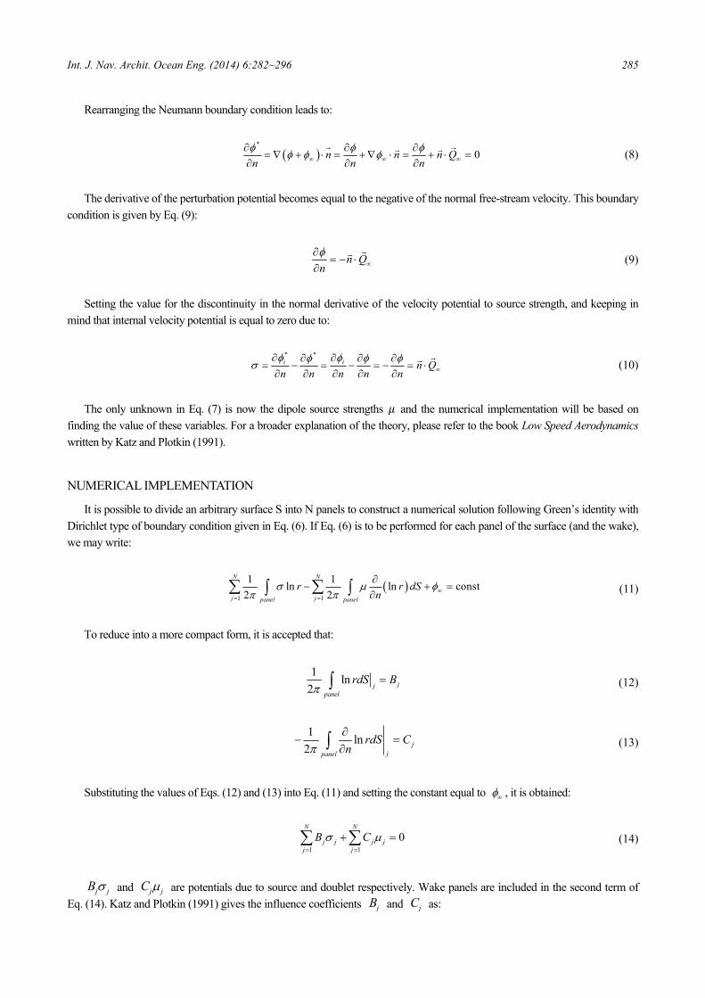
Int. J. Nav. Archit. Ocean Eng. (2014) 6:282~296 285
Rearranging the Neumann boundary condition leads to:
*
0n n n Qn n n
(8)
The derivative of the perturbation potential becomes equal to the negative of the normal free-stream velocity. This boundary
condition is given by Eq. (9):
n Qn
(9)
Setting the value for the discontinuity in the normal derivative of the velocity potential to source strength, and keeping in
mind that internal velocity potential is equal to zero due to:
* *i i n Q
n n n n n
(10)
The only unknown in Eq. (7) is now the dipole source strengths and the numerical implementation will be based on
finding the value of these variables. For a broader explanation of the theory, please refer to the book Low Speed Aerodynamics
written by Katz and Plotkin (1991).
NUMERICAL IMPLEMENTATION
It is possible to divide an arbitrary surface S into N panels to construct a numerical solution following Green’s identity with
Dirichlet type of boundary condition given in Eq. (6). If Eq. (6) is to be performed for each panel of the surface (and the wake),
we may write:
1 1
1 1ln ln const
2 2
N N
j jpanel panel
r r dSn
(11)
To reduce into a more compact form, it is accepted that:
1ln
2 jjpanel
rdS B
(12)
1ln
2 jjpanel
rdS Cn
(13)
Substituting the values of Eqs. (12) and (13) into Eq. (11) and setting the constant equal to , it is obtained:
1 1
0N N
j j j jj j
B C
(14)
j jB and j jC are potentials due to source and doublet respectively. Wake panels are included in the second term of
Eq. (14). Katz and Plotkin (1991) gives the influence coefficients jB and jC as:
286 Int. J. Nav. Archit. Ocean Eng. (2014) 6:282~296
2 2 2 21 1 2 2
1 1
2 1
1{( ) ln[( ) ] ( ) ln[( ) ]
4
2 (tan tan )}
j j j j j
j j
B x x x x z x x x x z
z zz
x x x x
(15)
1 1
2 1
1tan tan
2jj j
z zC
x x x x
(16)
Applying the Neumann boundary condition:
j jn Q (17)
Examining Eq. (14), it may be observed that the only unknown in the equation becomes the doublet strengths j .
Writing this equation N times (for the number of panels), a matrix equation is obtained with the right hand side equal to zero.
Getting j jB to the right hand side together with the inverse of the matrix jC , unknown j will be found of the body
and the wake.
After the derivation of doublet strengths, potential and velocities at each point inside the flow can be found by finite
difference method.
Ground may be represented by the image method as a numerical approximation to the real case. Image method states that if
a ground is present underneath an object inside the flow, the effect of the ground can be calculated by taking into account the
image of the real object (Katz and Plotkin, 1991). Please refer to Fig. 2 for a better presentation. In that Figure, a NACA6409
wing with 0° angle of attack is in ground proximity.
In this study, method of images was implemented to both direct and iterative boundary element methods for the repre-
sentation of the ground effect. It is accepted that ground effect in this article covers land only. WIG crafts can also operate
over water, however; due to approximately 1/800 density ratio of the air to the water, the water behaves like land in this situ-
ation. There may be a small decrease in the lift when operating over water but this is of small importance and can be neglected.
To understand the effects of the free water surface to a wing-in-ground effect, please refer to Liang and Zong (2011) and
Zong et al. (2012). To comprehend the free surface deformation at high Froude numbers for a wing-in-ground effect, please
see Barber’s numerical work (Barber, 2007).
(a) (b)
Fig. 2 NACA6409 wing-in-ground effect (a) and method of images approach for numerical calculations (b).
Int. J. Nav. Archit. Ocean Eng. (2014) 6:282~296 287
Direct boundary element method
The geometries inside the flow will be divided into panels and in each panel, there will be collocation points at which all the
calculations will be made. On each collocation point, constant strength sources and constant strength doublets will be distri-
buted and at all these collocation points Eq. (14) must be satisfied. Let’s say a body inside the fluid has N panels. Due to method
of images, there will be a total of 2N panels to be solved for which in total makes a 2 2N N matrix. Therefore, in this
matrix a total of 24N elements will be stored using computer memory.
Iterative boundary element method
When objects in the flow have complex shapes and must be represented by large amounts of panels, the sufficiency of a com-puter may be questioned. For example, if 1000N , then a total of 2000 panels must be solved to represent the ground effect. In this case, the conventional direct method will cover 4 million elements inside the matrix. The number of elements in the ma-trix will grow with the square of the number of panels and the computer will respond to give a solution to the problem slower.
An alternative method is the iterative boundary element method which suggests solving the problem separately. In the itera-tive approach, the problem is broken into parts to solve for each part separately; and then is reunited to go for a final solution.
With this approach, the real wing which is in ground proximity is solved first as if it is inside an unbounded fluid. The doublet strengths and the induced potentials by the wing in the outer flow are calculated. Then, the image wing is solved as if it is inside an unbounded fluid. However this time, off-body potentials induced by the real wing are added to the potentials induced by the image wing to integrate the effects of the interaction of the real wing with the ground. What is done here is the superposition of the flow around the image wing in an unbounded fluid with the effects induced by the real wing. After this step, attention turns to the real wing. Off-body potentials induced by the image wing on the real wing are added to the flow around the real wing in unbounded fluid. With this step, the effect of ground proximity is reflected to the real wing. Here; 1 jB , 1jC and 2 jC are the influence coefficients; while 1j , 1 j , 2 j and 2 j are the source and doublet strengths of the 1st and 2nd bodies respectively. 1jRHS and 2 jRHS refer to the right hand sides. Doing these calculations a number of times, convergence will be achieved after several iterations (Kinaci et al., 2012). Fig. 3 depicts the procedure of the developed code for the iterative approach to the problem while equation set (18) explains this mathematically.
• 1 1 1j j jC RHS
• 1 1 1j j jRHS B
START ITERATION
• 2 2 2j j jC RHS
• 2 2 2 1
1
j j j j
j
RHS B CI
BI
(Total potential acting on the 2nd body)
• 1 1 1j j jC RHS
• 1 1 1 2
2
j j j j
j
RHS B CI
BI
(Total potential acting on the 1st body)
RESTART ITERATION
STOP IF < (desired error)
(18)
Fig. 3 A scheme of the developed code.
288 Int. J. Nav. Archit. Ocean Eng. (2014) 6:282~296
Iterative boundary element method has a wide range of applicability from electromagnetism to heat transfer. It is also used
for fluid flow problems as Bal (2003; 2007; 2008; 2011) has selected works on the topic. However; the emergence and widely
usage of the IBEM dates back to 1990’s when Lesnic et al. (1997) have proposed the method for the solution of the Cauchy
problem for the Laplace equation, Up to now, IBEM has been used in many different fields and proved its worth in time.
VALIDATION
Validation with the single case
A wing in ground effect loses its advantage as it moves away from the ground. At infinite clearance, the wing will act like as if it is inside an unbounded fluid. If the ground is adequately far enough from the hydrofoil, then we must expect the hydrofoil to have its naked lift (as if there was nothing affecting the flow of the hydrofoil). To validate the results, a wing section of NACA6409 was chosen with the ground clearance selected to be 10h c in this section; which is thought to be far enough for the hydrofoil to interact.
The lift coefficients obtained at various angle of attacks for 10 c clearance and for the single case are given in Table 1.
The error percentage defined here is calculated as;
Singlecase Wingin groundeffect% 100
SinglecaseError
Table 1 Lift coefficients obtained for WIG effect and the single case.
AoA WIG effect Single case Error %
0 0.7329 0.734 0.15
2 0.9649 0.9637 0.12
4 1.1934 1.1982 0.4
6 1.4218 1.4305 0.61
8 1.6458 1.6603 0.87
Table 1 points out the precision the IBEM produces as the maximum error generated is less than 1%. The graphical view of
table 1 is given in Figs. 4-6 shows the negative pressure coefficient distribution for 0° and 8° of angle of attack obtained both
ways respectively.
Fig. 4 Graphical view of lift coefficients obtained both Fig. 5 Negative pressure coefficient distribution
ways (Clearance is 10 c for WIG effect). obtained both ways for 0° of AoA.
x
x
x
x
x
angle of attack
liftc
oeffi
cien
t
0 2 4 6 8
0.6
0.8
1
1.2
1.4
1.6
1.8
2
Single caseWIG effectx
xxxxxxxxxxxxxxxxxxxxxxxxxxxxxxxxxxxxxxxxxxx
xxxx
x
x
x
x
x
x
xxxxxxxxxxx x x x x x x x x x x x x x x x x x x x xxxxxxxxxxxxxx
xxxx
xxxx
xxxxxxxxxxxxxxxxxxxxxxxxxxxxxxxxx
xx
xxx
x
x
x
x
x
xxxxxxxxxxxxxx x x x x x x x x x x x x x x x x x x x xxxxxxxxxxxxxxx
x / c
-Cp
0 0.2 0.4 0.6 0.8 1-1
-0.5
0
0.5
1
Single case - 0 degreesW IG effect - 0 degreesx
Int. J. Nav. Archit. Ocean Eng. (2014) 6:282~296 289
Fig. 6 Negative pressure coefficient distribution obtained both ways for 8° of AoA.
Validation with direct BEM and CFD
As a first step, results derived with the boundary element and the Finite Volume Methods (FVM) were compared for a
single NACA6409 with an angle of attack of 4° in an unbounded fluid. Due to the absence of the ground effect, direct BEM
was used. Obtained lift coefficient values were in good agreement as BEM found 1.1982 while FVM found 1.1857 for the
wing. Fig. 7 shows the negative pressure coefficient distribution derived with BEM and CFD. Except the leading edge region
of the suction side, both methods gave compatible results with each other.
To prove the effectiveness of the IBEM, the obtained results are compared with the results obtained with Direct BEM
and CFD. This time, the same wing section was solved with ground clearance 0.20h c and the obtained results are given
in Fig. 8. IBEM produced 1.405 for the lift coefficient of the wing while Direct BEM and FVM generated 1.398 and 1.325
respectively.
Analyzing Fig. 8 will lead to the conclusion that IBEM is as strong as Direct BEM as the values found with both methods
overlap. Overall, IBEM shows up to be a good alternative to Direct BEM and FVM.
Fig. 7 Results of BEM and FVM in an unbounded fluid. Fig. 8 Results of IBEM, Direct BEM and
FVM for 0.02 c ground clearance.
xxxxxxxxxxxxxxxxxxxxxxxxxxxxxxxxxxxxxxxxxxxxxxxx
x
x
xx
x
xxxxxxxxxxxx x x x x x x x x x x x x x x x x x xxxxxxxxxxxxxxxxxxxx
xxxxxxxxxxxxxxxxxxxxxxxxxxxxxxxxxxxxxxxx
xxx
x
xx
x
x
xxxxx
xxxxxxxxxx x x x x x x x x x x x x x x x x x xxxxxxxxxxxxxxxx
290 Int. J. Nav. Archit. Ocean Eng. (2014) 6:282~296
Validation with results from the literature
Up to now, results found with IBEM seems to be in good agreement with the other methods. At this part of the paper, the
results produced with the iterative method will be compared with the results found in the literature. This will be done in two
steps. First, the lift coefficients produced with IBEM will be compared with Abramowski’s (2007) work and then the pressure
distribution will be compared with the results produced by Firooz and Gadami (2006).
Abramowski (2007) have investigated the ground effect over a NACA/Munk M15 airfoil. Lift coefficients at different
ground clearances have been found. Results found with IBEM is compared with the results in that study and this is given in
Fig. 9.
Fig. 9 Comparison of lift coefficients of Fig. 10 Comparison of pressure coefficient
NACA/Munk M15 airfoil. distribution over NACA4412 airfoil.
Although the results produced by IBEM is slightly lesser than Abramowski’s (2007) results, they pretty seem to be in accordance.
Pressure coefficient distribution along a NACA4412 airfoil is compared with Firooz and Gadami’s (2006) work. Fig. 10
exhibits this comparison and the results are again compatible.
TIME CONSUMPTIONS
Applicability of the iterative method relies on the results of time consumption. Iterative boundary element method will be
preferred in problems containing high number of panels which will give solutions slower. IBEM stores fewer values in the
computer’s memory while the direct boundary element uses more computer memory. This difference between the stored values
of both methods leads to differences in the acquisition of a solution. IBEM responds more quickly and gives faster results
(Kinaci et al., 2011).
To fully comprehend the advantage IBEM offers, a test case of a two dimensional NACA6409 wing with 0° AoA in ground
effect was solved in different clearances from the ground for various numbers of panels. The results of the test case are given in
Table 2.
Distances in Table 2 are dimensionless and given in /h c . The data of elapsed time for a specific panel number and dis-
tance are given in seconds. Both methods are tested under the same conditions in an average computer of Intel Core2 Duo CPU
E8500 @ 3.16GHz (32bit) with 4GB of RAM. /h c increases from 0.10 to 0.30 while panel number increases from 100 to
500. IBEM dominates direct BEM in terms of time consumption in all panel numbers and distances. The solutions are around
the same up to 0.15h with iterative method having a slight advantage against the direct method. However, there becomes a
major advantage after 0.20h . This means that as the clearance from the ground increases, the iterative method saves greater
h / c
Cl
0 0.1 0.2 0.3 0.4 0.5 0.6 0.70
0.2
0.4
0.6
0.8
1
Abramowski, 2007Present Study
xxxxxxxxxxxxxxxxxxxxxxxxxxxxxxxxxxxxxxxxxxxxxxxx
x
x
x
xxxxxxxxxxxxxxx x x x x x x x x x x x x x x x xxxxxxxxxxxxxxxxxxxx
xxxxxx
xxxxxxxxxxxxxxxxxxxxxxxxxxxxxxxxxxx
xxxxx
x
x
x
xxxxxx
xxxxxxxxxxx x x x x x x x x x x x x x x xxxxxxxxxxxxxxxxx
x / c
-Cp
0 0.2 0.4 0.6 0.8 1-1
-0.5
0
0.5
1
1.5
2
2.5
Firooz & GadamiPresent Studyx
Int. J. Nav. Archit. Ocean Eng. (2014) 6:282~296 291
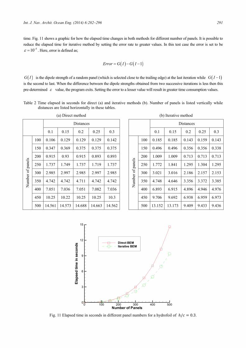
time. Fig. 11 shows a graphic for how the elapsed time changes in both methods for different number of panels. It is possible to
reduce the elapsed time for iterative method by setting the error rate to greater values. In this test case the error is set to be 510 . Here, error is defined as;
1Error G I G I
G I is the dipole strength of a random panel (which is selected close to the trailing edge) at the last iteration while 1G I
is the second to last. When the difference between the dipole strengths obtained from two successive iterations is less then this
pre-determined value, the program exits. Setting the error to a lesser value will result in greater time consumption values.
Table 2 Time elapsed in seconds for direct (a) and iterative methods (b). Number of panels is listed vertically while distances are listed horizontally in these tables.
Int. J. Nav. Archit. Ocean Eng. (2014) 6:282~296 293
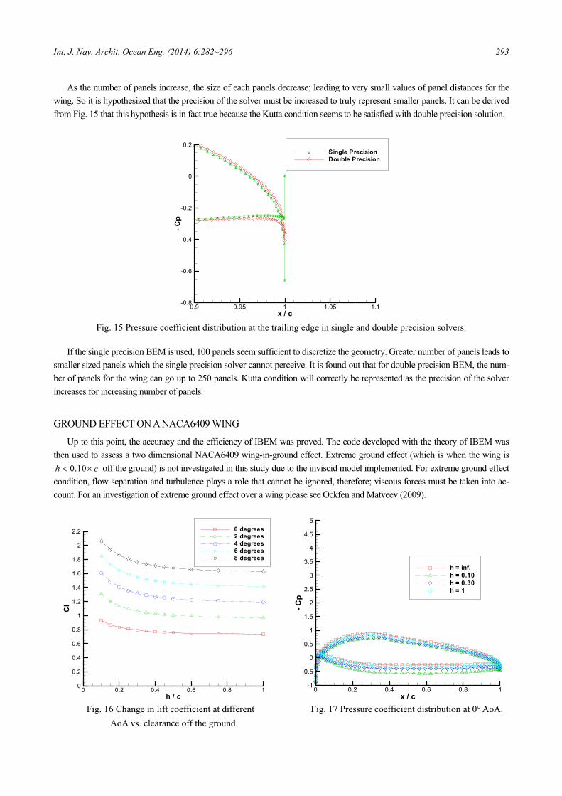
As the number of panels increase, the size of each panels decrease; leading to very small values of panel distances for the
wing. So it is hypothesized that the precision of the solver must be increased to truly represent smaller panels. It can be derived
from Fig. 15 that this hypothesis is in fact true because the Kutta condition seems to be satisfied with double precision solution.
Fig. 15 Pressure coefficient distribution at the trailing edge in single and double precision solvers.
If the single precision BEM is used, 100 panels seem sufficient to discretize the geometry. Greater number of panels leads to
smaller sized panels which the single precision solver cannot perceive. It is found out that for double precision BEM, the num-
ber of panels for the wing can go up to 250 panels. Kutta condition will correctly be represented as the precision of the solver
increases for increasing number of panels.
GROUND EFFECT ON A NACA6409 WING
Up to this point, the accuracy and the efficiency of IBEM was proved. The code developed with the theory of IBEM was
then used to assess a two dimensional NACA6409 wing-in-ground effect. Extreme ground effect (which is when the wing is
0.10h c off the ground) is not investigated in this study due to the inviscid model implemented. For extreme ground effect
condition, flow separation and turbulence plays a role that cannot be ignored, therefore; viscous forces must be taken into ac-
count. For an investigation of extreme ground effect over a wing please see Ockfen and Matveev (2009).
Fig. 16 Change in lift coefficient at different Fig. 17 Pressure coefficient distribution at 0° AoA.
AoA vs. clearance off the ground.
z
zzzzzzzzzzzzzzzzzzzzzzzz
zz
zz
zz
zz
zz
zz
zz
zz
zz
zzzz
zz
z
z
x / c
-Cp
0.9 0.95 1 1.05 1.1-0.8
-0.6
-0.4
-0.2
0
0.2Single PrecisionDouble Precision
z
h / c
Cl
0 0.2 0.4 0.6 0.8 10
0.2
0.4
0.6
0.8
1
1.2
1.4
1.6
1.8
2
2.2 0 degrees2 degrees4 degrees6 degrees8 degrees
x / c
-Cp
0 0.2 0.4 0.6 0.8 1-1
-0.5
0
0.5
1
1.5
2
2.5
3
3.5
4
4.5
5
h = inf.h = 0.10h = 0.30h = 1
294 Int. J. Nav. Archit. Ocean Eng. (2014) 6:282~296
The calculations are made for five different AoA values which are 0°, 2°, 4°, 6° and 8°. The solver is set to single precision, discretizing each wing with 100 panels. The change in lift coefficient at different AoA values is given in Fig. 16 The wing creates more lift as it gets closer to the ground. As the AoA of the wing increases, the wing shows tendency to create more lift in lower ground clearances. The curves get steeper as the AoA increases. Please see Fig. 16 for a better view.
Fig. 18 Pressure coefficient distribution at 4° AoA. Fig. 19 Pressure coefficient distribution at 8° AoA.
Negative pressure coefficient distributions along the NACA6409 wing in different ground clearances are given in Figs. 17,
18 and 19 for 0°, 4° and 8° of AoA respectively. In Figs. 17-19; the difference between the suction and the pressure side of the wing increases as the wing has higher AoA
which explains the reason of higher lift. The pressure coefficient distribution tends to get closer to the condition of unbounded fluid (which is the case of h ). Analyzing these Figs, it may be said that flow velocity over the wing (at both suction and pressure sides), are reduced. However; due to a higher reduction of flow velocity (and therefore a higher increase in the pressure) at the pressure side, the wing obtains more lift in ground proximity.
The increase in AoA sharply leads to an increase in the flow velocity at the leading edge. Ground proximity for a wing also plays a role in the rise of fluid velocity at this part of the wing. Although viscous forces are not included in this study, this explains the flow separation incident. When there is a big difference in velocities (or pressures) at two neighbor points on a body, the flow cannot follow the body surface and separates. Vortex motions may be formed which will lead the case to un-steady flow and an unstable condition for the wing. Therefore; stall may show up earlier in ground proximity and this phenol-menon must especially be avoided in WIG crafts. Stall of the wing will cause the craft to oscillate causing danger and discomfort for the passengers. Please refer to Fig. 20.
Fig. 20 A close up view of Fig. 19 at the leading edge.
x / c
-Cp
0 0.2 0.4 0.6 0.8 1-1
-0.5
0
0.5
1
1.5
2
2.5
3
3.5
4
4.5
5
h = inf.h = 0.10h = 0.30h = 1
x / c
-Cp
0 0.2 0.4 0.6 0.8 1-1
0
1
2
3
4
5
h = inf.h = 0.10h = 0.30h = 1
x / c
-Cp
0.01 0.012 0.0144
4.2
4.4
4.6
4.8
5
h = inf.h = 0.10
Pre
ssur
edi
ffere
nce
forh
=in
f.
Pre
ssur
edi
ffere
nce
forh
=0.
10
Int. J. Nav. Archit. Ocean Eng. (2014) 6:282~296 295
For high AoA conditions of the wing in closer ground proximities, it is suggested that unsteady IBEM to be used to detect
oscillations and vortex formations around the wing. This way, the lift and the pressure around the wing can be retained more
precisely.
CONCLUSION AND FUTURE WORK
In this paper, an iterative boundary element method for a solution of the flow around a wing-in-ground effect was pro-
posed. Compared to RANSE solutions BEM is quite faster; which only discretizes the body inside the fluid rather than the
whole fluid domain. However, as shown in this paper, there are methods to increase the efficiency of BEM. Iterative BEM is
faster and has good precision, therefore; it seems to be more efficient than direct BEM. Iterative method shows good prospect
in dealing with geometries in ground proximity where a higher number of panels must be used. These may include complex
bodies of three dimensions in which case the panels will no longer be represented by lines but surfaces which will increase the
calculation time significantly. Quick assessment of the efficiency of a particular type of wing section for WIG crafts can be
made with IBEM.
When the wing is in extreme ground effect, the wing will possibly oscillate in the air due to vortex separations from the
body. This will create unsteady motions for the wing. Unsteady motions will lead the WIG problem to be solved at each time
step increasing the necessity for quicker solutions. It is thought that IBEM will prove its real worth in unsteady cases where the
solution time is expected to drop significantly. As a future work, the generated code will be developed for solving unsteady
motions to include extreme ground effect cases.
ACKNOWLEDGEMENT
This research has been supported by Yildiz Technical University Scientific Research Projects Coordination Department.
Project No: 2013-10-01-KAP02. The author feels gratitude towards Prof. Sakir BAL due to his generous aids while developing
the code and Prof. Mesut GUNER for supporting the work.
REFERENCES
Abramowski, T., 2007. Numerical investigation of airfoil in ground proximity. Journal of Theoretical and Applied Me-
chanics, 45(2), pp.425-436.
Ahmed, M.R. and Sharma, S.D., 2005. An investigation on the aerodynamics of a symmetrical airfoil in ground effect. Ex-
perimental Thermal and Fluid Science, 29(6), pp.633-647.
Bal, S., 2003. A numerical wave tank model for cavitating hydrofoils. Computational Mechanics, 32(4-6), pp.259-268.
Bal, S., 2007. A numerical method for the prediction of wave pattern of surface piercing cavitating hydrofoils. Proceedings
of the Institution of Mechanical Engineers Part C-Journal of Mechanical Engineering Science, 221(12), pp.1623-1633.
Bal, S., 2008. Prediction of wave pattern and wave resistance of surface piercing bodies by a boundary element method.
International Journal for Numerical Methods in Fluids, 56(3), pp.305-329.
Bal, S., 2011. The effect of finite depth on 2D and 3D cavitating hydrofoils. Journal of Marine Science and Technology,
16(2), pp.129-142.
Barber, T.J., 2007. A study of water surface deformation due to tip vortices of a wing-in-ground effect. Journal of Ship Re-
search, 51(2), pp.182-186.
Daichin, K.W., 2007. PIV measurements of the near-wake flow of an airfoil above a free surface. Journal of Hydrodyna-
mics, 19(4), pp.482-487.
Djavareshkian, M.H., Esmaeli, A. and Parsani, A., 2010. Aerodynamics of smart flap under ground effect. Aerospace Sci-
ence and Technology, 15(8), pp.642-652.
Firooz, A. and Gadami, M., 2006. Turbulence flow for NACA 4412 in unbounded flow and ground effect with different
turbulence models and two ground conditions; fixed and moving ground conditions. BAIL 2006, Germany, 23-28 July
2006, pp.81-84.
296 Int. J. Nav. Archit. Ocean Eng. (2014) 6:282~296
Halloran, M. and O’Meara, S., 1999. Wing in ground effect craft review. [pdf] Melbourne: DSTO Aeronautical and Mari-
time Research Laboratory. Available at: < http://www.dtic.mil/cgi-bin/GetTRDoc?AD=ADA361836 > [Accessed 29
July 2013].
Jamei, S., Maimun, A., Mansor, S., Azwadi, N. and Priyanto, A., 2012. Numerical investigation on aerodynamic charac-
teristics of a compound wing-in-ground effect. Journal of Aircraft, 49(5), pp.1297-1305.
Jung, K.H., Chun, H.H. and Kim, H.J., 2008. Experimental investigation of wing-in-ground effect with a NACA6409 sec-
tion. Journal of Marine Science and Technology, 13(4), pp.317-327.
Katz, J. and Plotkin, A., 1991. Low speed aerodynamics-from wing theory to panel methods. 1st ed. Singapore: Mc-Graw
Hill Inc.
Kim, H.J., Chun, H.H. and Kwang, H.J., 2009. Aeronumeric optimal design of a wing-in-ground-effect craft. Journal of
Marine Science and Technology, 14(1), pp.39-50.
Kinaci, O.K., Kukner, A. and Bal, S., 2011. Interactive effects of 2-D bodies in non-lifting flows. INT-NAM 2011, Turkey,
24-25 October 2011, pp.817-826.
Kinaci, O.K., Kukner, A. and Bal, S., 2012. A parametric study on tandem hydrofoil interaction. HYDMAN 2012, Poland,
19-20 September 2012, pp.145-155.
Lee, J., Han, C.S. and Bae, C.H., 2010. Influence of wing configurations on aerodynamic characteristics of wings in ground
effect. Journal of Aircraft, 47(3), pp.1030-1040.
Lesnic, D., Elliott, L. and Ingham, D.B., 1997. An iterative boundary element method for solving numerically the Cauchy
problem for the Laplace equation. Engineering Analysis with Boundary Elements, 20(2), pp.123-133.
Liang, H. and Zong, Z., 2011. A subsonic lifting surface theory for wing-in-ground effect. Acta Mechanica, 219(3-4),
pp.203-217.
Liang, H., Zhou, L., Zong, Z. and Sun, L., 2013. An analytical investigation of two-dimensional and three-dimensional
biplanes operating in the vicinity of a free surface. Journal of Marine Science and Technology, 18(1), pp.12-31.
Luo, S.C. and Chen, Y.S., 2012. Ground effect on flow past a wing with a NACA0015 cross-section. Experimental Ther-
mal and Fluid Science, 40, pp.18-28.
Ockfen, A.E. and Matveev, K.I., 2009. Aerodynamic characteristics of NACA4412 airfoil section with flap in extreme gro-
und effect. International Journal of Naval Architecture and Ocean Engineering, 1(1), pp.1-12.
Phillips, W.F. and Hunsaker, D.F., 2013. Liftring-line predictions for induced drag and lift in ground effect. Journal of Air-
craft, 50(4), pp.1226-1233.
Reeves, J.M.L., 1993. The case for surface effect research, platform applications and development opportunities. In: NATO-
A-GARD fluid mechanics panel (FMP) symposium in long range and long range endurance operation of aircraft, 24-