AN ITERATIVE SIGNAL DETECTION ALGORITHM BASED ON BAYESIAN BELIEF PROPAGATION IDEAS I. Proudler ∗ QinetiQ Ltd. St Andrews Road, Malvern Worcestershire, WR14 2NJ S. Roberts, S. Reece and I. Rezek Dept. of Engineering Science University of Oxford, Parks Road, Oxford, OX1 3PJ ABSTRACT We investigate the construction of an iterative algorithm for signal detection based on Pearl’s Belief Propagation algorithm. Two main issues arise: the need to modify the graphical model of the problem in order to force the creation of an iterative algorithm, and the need to find suitable approximations to various probability distribution functions so as to allow an efficient implementation of the algorithm. The resulting al- gorithm is similar to a conventional deflation-based approach but it can make soft rather than hard decisions. Index Terms— signal processing, iterative algorithms, Bayesian, belief propagation, Pearl’s algorithm. 1. INTRODUCTION Parameter estimation is at the heart of much of modern adap- tive digital signal processing. However most, if not all, prac- tical estimation problems involve nonlinear functions when expressed in an ideal form. This causes problems because the resulting mathematics is too difficult for a closed form solu- tion to be found. In order to develop an algorithm some sort of compromise in needed. One approach is to develop an itera- tive algorithm for example by spliting the problem into two or more sub-problems each of which can be solved given some estimates from the other sub-problems (deflation). The defi- ciency with this approach is that the resulting algorithm usu- ally only converges to the correct solution if the initial guess is close by. However when it does converge one has a means to solve the difficult nonlinear problem in a very efficient, ro- bust way. A recent example of a highly successful iterative estima- tion algorithm is the Turbo Code decoding algorithm [1]. It has been shown recently that the Turbo Code decoding algo- rithm is an instantiation of Pearl’s Belief Propagation algo- rithm [2]. In the following, we investigate the application of Pearl’s algorithm to a fairly generic, signal detection prob- lem. The motivation being to discover if a similarly powerful, iterative, detection algorithm can be created. ∗ This work was sponsored by the Royal Academy of Engineering, the ES Domain of the UK MOD’s Research Acquisition Organisation, and QinetiQ. 2. SIGNAL DETECTION 2.1. Introduction In this section we consider a problem that involves the de- tection of several signals, of known shape or ‘signature’, in noise. This is a common problem found, for example, in biomedical signal analysis, communications, radar and sonar. The observed data is given by y = T 1 (a 1 ,k 1 )+ T 2 (a 2 ,k 2 )+ w (σ) where w (σ) is Gaussian white noise, T i (a i ,k i )= a i f (k i ) and a i is the (unknown) signal amplitude, f () is the (known) signal response vector and k i is the (unknown) position pa- rameter. For simplicity we consider the case when the noise and the amplitude coefficients a i are real. Note that because a signal can be located at any position in the data and with any amplitude, the priors for this problem are uninformative. 2.2. Pearl’s Algorithm In a Bayesian inference problem one tries to estimate the pos- terior probability distribution of a set of variables given some measurements In general this is a complicated problem to solve but if the problem has structure then the posterior proba- bility distribution will factor into simpler elements. The struc- ture can be represented via a ‘graphica’ model: a directed graph where each node represents a variable and the links show the causal connections between the variables. Pearl’s algorithm calculates the marginal probabilities at the nodes based on ‘messages’ that are passed between the nodes [3]. 2.3. Iterative Algorithm Design The graphical model for the detection problem is shown in figure 1(a). The nodes labelled a i and k i represent the am- plitude and position parameters, respectively, of the two sig- nals. The nodes labelled T 1 and T 2 represent the contribution of each of the two signals to the observed data (i.e. a i f (k i )),
Transcript
AN ITERATIVE SIGNAL DETECTION ALGORITHM BASED ON BAYESIAN BELIEFPROPAGATION IDEAS
ABSTRACTWe investigate the construction of an iterative algorithm forsignal detection based on Pearl’s Belief Propagation algorithm.Two main issues arise: the need to modify the graphical modelof the problem in order to force the creation of an iterativealgorithm, and the need to find suitable approximations tovarious probability distribution functions so as to allow anefficient implementation of the algorithm. The resulting al-gorithm is similar to a conventional deflation-based approachbut it can make soft rather than hard decisions.
Index Terms— signal processing, iterative algorithms,Bayesian, belief propagation, Pearl’s algorithm.
1. INTRODUCTION
Parameter estimation is at the heart of much of modern adap-tive digital signal processing. However most, if not all, prac-tical estimation problems involve nonlinear functions whenexpressed in an ideal form. This causes problems because theresulting mathematics is too difficult for a closed form solu-tion to be found. In order to develop an algorithm some sort ofcompromise in needed. One approach is to develop an itera-tive algorithm for example by spliting the problem into two ormore sub-problems each of which can be solved given someestimates from the other sub-problems (deflation). The defi-ciency with this approach is that the resulting algorithm usu-ally only converges to the correct solution if the initial guessis close by. However when it does converge one has a meansto solve the difficult nonlinear problem in a very efficient, ro-bust way.
A recent example of a highly successful iterative estima-tion algorithm is the Turbo Code decoding algorithm [1]. Ithas been shown recently that the Turbo Code decoding algo-rithm is an instantiation of Pearl’s Belief Propagation algo-rithm [2]. In the following, we investigate the application ofPearl’s algorithm to a fairly generic, signal detection prob-lem. The motivation being to discover if a similarly powerful,iterative, detection algorithm can be created.
∗This work was sponsored by the Royal Academy of Engineering, the ESDomain of the UK MOD’s Research Acquisition Organisation, and QinetiQ.
2. SIGNAL DETECTION
2.1. Introduction
In this section we consider a problem that involves the de-tection of several signals, of known shape or ‘signature’, innoise. This is a common problem found, for example, inbiomedical signal analysis, communications, radar and sonar.
The observed data is given by
y = T 1 (a1, k1) + T 2 (a2, k2) + w (σ)
where w (σ) is Gaussian white noise, T i (ai, ki) = aif (ki)and ai is the (unknown) signal amplitude, f () is the (known)signal response vector and ki is the (unknown) position pa-rameter. For simplicity we consider the case when the noiseand the amplitude coefficients ai are real. Note that because asignal can be located at any position in the data and with anyamplitude, the priors for this problem are uninformative.
2.2. Pearl’s Algorithm
In a Bayesian inference problem one tries to estimate the pos-terior probability distribution of a set of variables given somemeasurements In general this is a complicated problem tosolve but if the problem has structure then the posterior proba-bility distribution will factor into simpler elements. The struc-ture can be represented via a ‘graphica’ model: a directedgraph where each node represents a variable and the linksshow the causal connections between the variables. Pearl’salgorithm calculates the marginal probabilities at the nodesbased on ‘messages’ that are passed between the nodes [3].
2.3. Iterative Algorithm Design
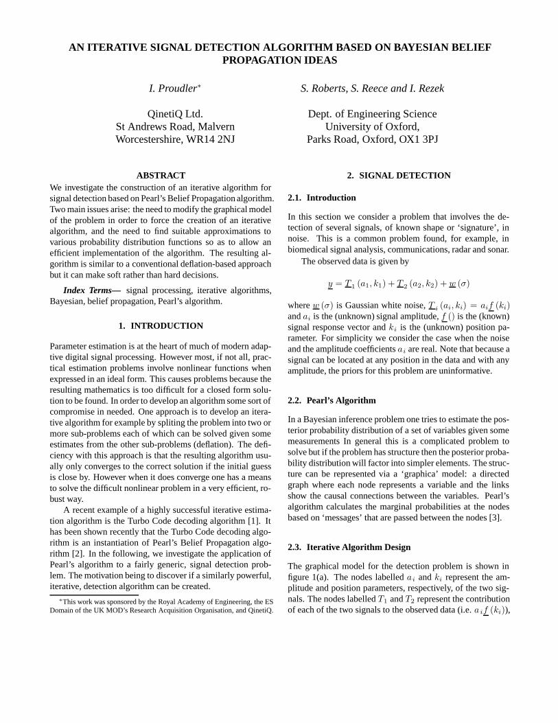
The graphical model for the detection problem is shown infigure 1(a). The nodes labelled ai and ki represent the am-plitude and position parameters, respectively, of the two sig-nals. The nodes labelled T1 and T2 represent the contributionof each of the two signals to the observed data (i.e. a if (ki)),
(a) Basic Model (b) Alternative Model
Fig. 1. Graphical Models for Signal Detection Problem
the node labelled λ represents the noise1 and the node labelledY represents the observed data. It can readily be seen fromfigure 1(a) that the graph is a tree. This means that Pearl’s al-gorithm for this problem is not iterative [3]. Furthermore it isrelatively easy to see that the resulting algorithm is rather triv-ial: The belief in a given signal effectively reduces to a state-ment of Bayes’ rule with the other signals marginalised out ofthe problem. However we do not have informative priors sothe algorithm tries to detect each signal under the assumptionthat it is the only one present.
In contrast we know [2] that Pearl’s algorithm for theTurbo-Code decoding problem produces the iterative algo-rithm of Berrou et al. [1]. The iterative nature of the Berrou’salgorithm is a result of the fact that the graphical model hasloops [4]. By adding a second data node to the graph for thedetection problem (figure 1(b)) we create a ‘loopy’ graphicalmodel similar to that of the Turbo-Code problem [2]. If a sec-ond set of data was avalable it would be attached to this newnode. If not, we duplicate the observed data and ignore thestatistical dependence between the two copies. Despite thepossible dangers with such an approach, as we shall see, itdoes in fact lead to a useful, non-trivial algorithm. The re-sulting algorithm is very similar to that for the Turbo Codedecoder ( [2]) but with the two decoder blocks replaced withestimation operations.
2.4. Computational Issues
Pearl’s algorithm is really a meta-algorithm in that it speci-fies, algebraically, how the probability distribution functionscan be calculated. For example we are required to evaluateintegrals such as∫ (
λ
2π
)N2
e−λ2 ‖(y−a1f(k1)−a2f(k2))‖2
πy (k1) dk1
that have no closed form solution. Furthermore the form ofthe various messages being passed in the algorithm can in
1For arithmetic reasons we deal with the variable λ = 1/σ2 instead of σ- the former being known as the ‘precision’.
principle change with each iteration. Hence the only way toimplement the algorithm correctly is via the use of numericaltechniques like sampling [5].
On the other hand, numerical Bayesian techniques arecomputationally very demanding. Thus it is highly desirableto be able to represent the message distributions by means ofsufficient statistics. For the detection example this is possi-ble provided some approximations are used. In particular, ifwe avoid having to evaluate integrals that involve nonlinearfunctions (see section 4) and require the πy (Ti) messages2 tobe multivariate Normal distributions and the πy (λ) is Gammadistributed, then a consistent allocation of distributions is pos-sible provided we use the approximations shown in section 3.The resulting algorithm is shown in table 1.
3. APPROXIMATE MESSAGE DISTRIBUTIONS
3.1. Introduction
We desire to approximate various parameterised functions byother parameterised functions. In the Bayesian literature theideal way to do this is to minimise the Kullbeck-Leibler di-vergence of the two functions. The KL divergence can bewritten:
KL (f (x|θ) , g (x|φ)) =∫
f (x|θ) ln(
f (x|θ)g (x|φ)
)dx
where the parameters θ are given and φ are to be determinedby the minimisation. Note that we do not need a good func-tional approximation but rather a good ‘information theoretic’one that captures the relevant information.
3.2. Normal-Gamma Approximation to Normal x Gamma
We require to find a Normal-Gamma approximation to theproduct πy (T )πy (λ) i.e. find (µ̄, L, α, β) that minimises
KL(N
(µ | µ̃, L̃
)Ga
(λ | α̃, β̃
), NG (µ, λ | µ̄, L, α, β)
)where N (), Ga () and NG () are Normal, Gamma and Normal-Gamma distributions respectively. It is not clear that a closedform solution to the KL minimisation problem exists. How-ever if we approximate Eλ {ln (λ)} by ln (Eλ {λ}), assumethat the logarithm function is approxiamtely constant, andalign the peak of the Normal-Gamma with that of the Gamma,the KL divergence is approximately minimised when µ̄ = µ̃,
L = Nβ̃L̃/α̃, α = rβ−N2 +1 and β = exp
((α̃β̃− r ln
(α̃β̃
))/r
)where r = α̃−1
β̃. The resulting approximation is good except
in the region where λ is small. The approximation capturesthe mean of µ correctly but the effect of the approximationerror is to underestimate the precision of the contribution of asignal to the observed data at low SNRs.
2The nodes a and b exchange the messages πa (b) and λb (a) - see [3]for definitions
0 50 1000
0.2
0.4
0.6
0.8
1 L=1000PeakApprox
(a) L = 10000 50 100
0
0.2
0.4
0.6
0.8
1
L=20PeakApprox
(b) L = 20
Fig. 2. Example of the Peak Approximation to λyi (λ) fordifferent values of L
3.3. Normal Approximation to Student t distribution
The message λy (T ) is a Student t distribution and we requirea Normal approximation for it. Minimising the KL diver-gence results in an intractable set of equations. On the otherhand, if we equate the mode of both distributions, in terms ofposition and height, and use Stirling’s approximation for thefactorial function, we get a good approximation to the Stu-dent t distribution - this is not surprising given the form of thetwo distributions:
St (x |µ, λ, α) ≈ N
(x |µ,
(λ
α
)e−1N
)
3.4. Gamma Approximation to Integral of a Gamma
We require a Gamma approximation(Ga
(λ | α̃, β̃
))for the
message λy (λ). Consider
λyi (λ) =∫
Ga
(λ | 3
2,∥∥∥x − µ̄ − µ
0
∥∥∥2)
N(µ | µ̄, L
)dµ
Minimising the KL divergence directly does not lead to atractable solution. Instead we set the position of the peak
of Ga(λ | α̃, β̃
)at the same point as the peak of λyi (λ),
and assume that Eλ {f (λ)} ≈ f (Eλ {λ}), the logarithm
function and(λ0β̃+1)
((λ0+L)β̃+1) are approximately constant, then
we have that α̃ = λ0β̃ and β =∥∥∥x −
(µ̄ + µ
0
)∥∥∥2
where
λ0 = NL(Lβ−N) . If L is large, λyi (λ) is very nearly a gamma
distribution (see figure 2-a) as we get a good approximation.Otherwise, λyi (λ) rises from zero to a constant value (seefigure 2-b) and represents little more than a lower bound on λand this is all that needs to be captured in the approximation.Note that there is no peak for the case L = 20 (see figure 2-b).so the position of the peak is limited to some (predetermined)maximum value.
4. SIGNATURE FUNCTION
Each λy (T ) message is represented as Normal distributionand therefore consists of a mean and precision. The mean isa representation of the contribution of this signal to the ob-served data. Ideally it should have the form af (k) where a
Inputs: µ1, λ1, µ2
, λ2, α, β,(µ
10, λ10, µ20
, λ20, α0, β0
)Calculation (j ∈ {1, 2})
Lj = Nβα λj ; c = α−1
β ; α̃ = cβ − N2 + 1
β̃ = exp
(αβ −c ln(α
β )c
); µ
11= y − µ
2
λ11 = L2
β̃(L2+1)
(Γ( 1
2 (2α̃+N))Γ(α̃)
) 2N
µ21
= y − µ1
λ21 = L1
β̃(L1+1)
(Γ( 1
2 (2α̃+N))Γ(α̃)
) 2N
L = λ1λ2λ1+λ2
; r =∥∥∥y − µ
1− µ
2
∥∥∥2
λ0 =
{L0 if (Lr − N) ≤ 0min
(NL
Lr−N , L0
)otherwise
β1 = e−1λ0
; α1 = λ0β1 + 1
(xcj , aj , kj) = xcorr(µ
j, f ()
)(see section 4)
µ̄j
=λjµj+xcjλja[j]f(k[j])
λj+xcjλj; λ̄j = λj + xcjλj
µ′j
=λ̄j µ̄
j+λj1µ
j1+λj0µ
j0
λ̄j+λj1+λj0; λ′
j = λ̄j + λj1 + λj0
α′ = α + α1 + α0; β′ = β + β1 + β0
Outputs: µ′1, λ′
1, µ′2, λ′
2, α′, β′
Table 1. ’Turbo’ Signal Detection Algorithm
and k are as yet unknown. One way in which a and k can beestimated is by correlating the mean with the signature func-tion. The position of the peak of the correlation function givesan estimate of k and an estimate of a can be found from itsmaximum value.
Having generated an estimate of a and k, we now have tomodify the λy (T ) message accordingly. This done via Bayestheorem. That is we consider the original λy (T ) message tobe a likelihood and the estimate of the signal response basedon a and k as the prior, then the updated message is the pos-terior. The prior (p (T )) can be modelled as a Normal distri-bution with mean af (k). If the mean of the original λy (T )message and af (k) are dissimilar then we say that the preci-sion of the prior is low and vice versa. However if the meanof the original λy (T ) was erroneous, giving the time seriesaf (k) a large precision would be wrong even if the correla-tion coefficient were close to unity. Hence we choose to setthe precision of the prior equal to the correlation coefficienttimes the precision of the original λy (T ) message.
5. SIMULATION RESULTS
Some initial simulations were performed using the model de-scribed in section 2. As well as the new ‘Turbo’ algorithm aconventional deflationary algorithm was used. The data con-
0 20 40 60 80 100−0.4
−0.2
0
0.2
0.4
0.6
0.8
1
1.2
1.4
1.6DataTurbo Estimate
(a) Turbo Algorithm
0 20 40 60 80 100−0.4
−0.2
0
0.2
0.4
0.6
0.8
1
1.2
1.4
1.6DataConventional Estimate
(b) Conventional Algorithm
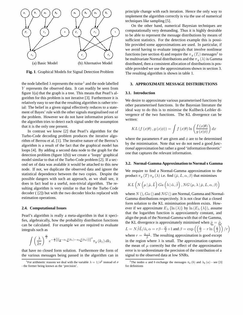
Fig. 3. Data and Signal Responses
sisted of 100 time samples and the signal signature f (k) wasa sinc function truncated to 15 time samples. Three signalswere place close together at time instants 45, 50 and 55 withamplitudes 1.1, 1.8 and 1.3 The noise had a variance of unity.In order to add some realism, two inaccuracies were intro-duced. The algorithms had no knowledge of the number ofsignals present: Both algorithms assumed there were at mostfive signals. The algorithms also used an incorrect signaturefunction: A sinc function was used where the width of thepeak is narrower than the real signatures. In this case the for-mula for the precision of the signal signature prior (see section4) was modified by weighting it by 0.5 to reflect the lack ofconfidence in the function being used.
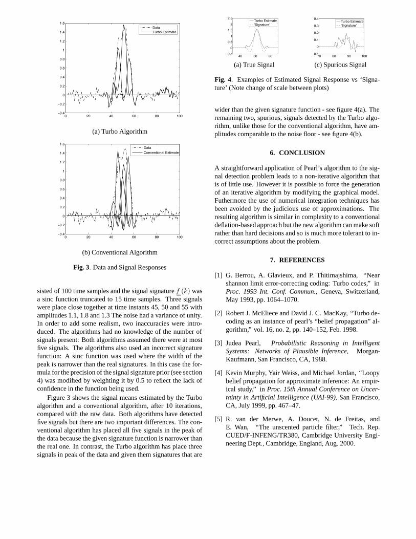
Figure 3 shows the signal means estimated by the Turboalgorithm and a conventional algorithm, after 10 iterations,compared with the raw data. Both algorithms have detectedfive signals but there are two important differences. The con-ventional algorithm has placed all five signals in the peak ofthe data because the given signature function is narrower thanthe real one. In contrast, the Turbo algorithm has place threesignals in peak of the data and given them signatures that are
40 50 60−0.5
0
0.5
1
1.5
2
2.5Turbo Estimate’Signature’
(a) True Signal
70 80 90 100−0.1
0
0.1
0.2
0.3
0.4Turbo Estimate’Signature’
(c) Spurious Signal
Fig. 4. Examples of Estimated Signal Response vs ‘Signa-ture’ (Note change of scale between plots)
wider than the given signature function - see figure 4(a). Theremaining two, spurious, signals detected by the Turbo algo-rithm, unlike those for the conventional algorithm, have am-plitudes comparable to the noise floor - see figure 4(b).
6. CONCLUSION
A straightforward application of Pearl’s algorithm to the sig-nal detection problem leads to a non-iterative algorithm thatis of little use. However it is possible to force the generationof an iterative algorithm by modifying the graphical model.Futhermore the use of numerical integration techniques hasbeen avoided by the judicious use of approximations. Theresulting algorithm is similar in complexity to a conventionaldeflation-based approach but the new algorithm can make softrather than hard decisions and so is much more tolerant to in-correct assumptions about the problem.
7. REFERENCES
[1] G. Berrou, A. Glavieux, and P. Thitimajshima, “Nearshannon limit error-correcting coding: Turbo codes,” inProc. 1993 Int. Conf. Commun., Geneva, Switzerland,May 1993, pp. 1064–1070.
[2] Robert J. McEliece and David J. C. MacKay, “Turbo de-coding as an instance of pearl’s “belief propagation” al-gorithm,” vol. 16, no. 2, pp. 140–152, Feb. 1998.
[3] Judea Pearl, Probabilistic Reasoning in IntelligentSystems: Networks of Plausible Inference, Morgan-Kaufmann, San Francisco, CA, 1988.
[4] Kevin Murphy, Yair Weiss, and Michael Jordan, “Loopybelief propagation for approximate inference: An empir-ical study,” in Proc. 15th Annual Conference on Uncer-tainty in Artificial Intelligence (UAI-99), San Francisco,CA, July 1999, pp. 467–47.
[5] R. van der Merwe, A. Doucet, N. de Freitas, andE. Wan, “The unscented particle filter,” Tech. Rep.CUED/F-INFENG/TR380, Cambridge University Engi-neering Dept., Cambridge, England, Aug. 2000.


![An Iterative Array Signal Segregation Algorithm · 2019-05-22 · niques such as multiple signal classification (MUSIC)[17]–[24] or estimation of signal parameters via rotational](https://static.documents.pub/doc/80x56/5f8ce6481a20566ac6297e84/an-iterative-array-signal-segregation-algorithm-2019-05-22-niques-such-as-multiple.jpg)


![IEEE TRANSACTIONS ON SIGNAL PROCESSING ...arXiv:0812.2324v1 [cs.IT] 12 Dec 2008 IEEE TRANSACTIONS ON SIGNAL PROCESSING (ACCEPTED) 1 The MIMO Iterative Waterfilling Algorithm Gesualdo](https://static.documents.pub/doc/80x56/5e27434f4ba58d386d0b08be/ieee-transactions-on-signal-processing-arxiv08122324v1-csit-12-dec-2008.jpg)

