138
ELEMENTS OF THE THEORY OF FUNCTIONS AND FUNCTIONAL ANALYSIS Volume 2 Measure The Lebesgue Integral Hilbert Space All. Kolmogorov and S. V. Fomin
| Date post: | 12-Jan-2016 |
| Category: |
Documents |
| Upload: | victorbr12 |
| View: | 34 times |
| Download: | 1 times |

ELEMENTS OF THE
THEORY OF
FUNCTIONS AND
FUNCTIONAL
ANALYSIS
Volume 2Measure
The Lebesgue IntegralHilbert Space
All. Kolmogorov and S. V. Fomin
ELEMENTS OF THE THEORY OF FUNCTIONS
AND FUNCTIONAL ANALYSIS
VOLUME
MEASURE. THE LEBESGUE INTEGRAL. HILBERT SPACE
OTHER GRAYLOCK PUBLICATIONS
KHINCHIN: Three Pearls of Number TheoryMathematical Foundations of Quantum Statistics
PONTRYAGIN: Foundations of Combinatorial Topology
NOVOZHILOV: Foundations of the Nonlinear Theory ofElasticity
KOLMOGOROV and FOMIN: Elements of the Theory of Functions andFunctional Analysis. Vol. 1: Metric andNormed Spaces
PETROVSKIT: Lectures on the Theory of Integral Equations
ALEKSANDROV: Combinatorial TopologyVol. 1: Introduction. Complexes. Coverings.DimensionVol. The Betti GroupsVol. 3: Homological Manifolds. The DualityTheorems. Cohomology Groups of Compacta.Continuous Mappings of Polyhedra
Elements of the Theoryof Functions
and Functional Analysis
VOLUME 2
MEASURE. THE LEBESGLTE INTEGRAL.HILBERT SPACE
BY
A. N. KOLMOGOROV AND S. V. FOMIN
TRANSLATED FROM THE FIRST (1960) RUSSIAN EDITIONby
HYMAN KAMEL AND HORACE KOMM
Department of MathematicsRensselaer Polytechnic Institute
GI?A YLOCKALBANY, N. Y.
1961
PRESS

Copyright © 1961
byGRAYLOCK PRESS
Albany, N. Y.
Second Printing—January 1963
All rights reserved. This book, or partsthereof, may not be reproduced in anyform, or translated, without permis-sion in writing from the publishers.
Library of Congress Catalog Card Number 57—4134
Manufactured in the United States of America

CONTENTS
Preface viiTranslators' Note ix
CHAPTER V
MEASURE THEORY
33. The measure of plane sets 1
34. Collections of sets 1535. Measures on semi-rings. Extension of a measure on a semi-ring to
the minimal ring over the semi-ring 2036. Extension of Jordan measure 2337. Complete additivity. The general problem of the extension of
measures 2838. The Lebesgue extension of a measure defined on a semi-ring with
unity 3139. Extension of Lebesgue measures in the general case 36
CHAPTER VI
MEASURABLE FUNCTIONS
40. Definition and fundamental properties of measurable functions.. 3841. Sequences of measurable functions. Various types of convergence. 42
CHAPTER VII
THE LEBESGUE INTEGRAL
42. The Lebesgue integral of simple functions 4843. The general definition and fundamental properties of the Lebesgue
integral 5144. Passage to the limit under the Lebesgue integral 5645. Comparison of the Lebesgue and Riemann integrals 6246. Products of sets and measures 6547. The representation of plane measure in terms of the linear meas-
ure of sections and the geometric definition of the Lebesgue in-tegral 68
48. Fubini's theorem 7249. The integral as a set function 77
V
CONTENTS
CHAPTER VIII
SQUARE INTEGRABLE FUNCTIONS
50. The spaceL2 7951. Mean convergence. Dense subsets of L2 8452. L2 spaces with countable bases 8853. Orthogonal sets of functions. Orthogonalization 9154. Fourier series over orthogonal sets. The Riesz-Fisher theorem. ... 9655. Isomorphism of the spaces L2 and 12 101
CHAPTER IX
ABSTRACT HILBERT SPACE. INTEGRAL EQUATIONSWITH SYMMETRIC KERNEL
56. Abstract Hilbert space 10357. Subspaces. Orthogonal complements. Direct sums 10658. Linear and bilinear functionals in Hilbert space 11059. Completely continuous self adjoint-operators in H 11560. Linear operator equations with completely continuous operators.. 11961. Integral equations with symmetric kernel 120SUPPLEMENT AND CORRECTIONS TO VOLUME 1 123INDEX 127

PREFACEThis book is the second volume of Elements of the Theory of Functions
and Functional Analysis (the first volume was Metric and Normed Spaces,Graylock Press, 1957). Most of the second volume is devoted to an ex-position of measure theory and the Lebesgue integral. These concepts,particularly the concept of measure, are discussed with some degree ofgenerality. However, in order to achieve greater intuitive insight, we beginwith the definition of plane Lebesgue measure. The reader who wishes todo so may, after reading §33, go on at once to Ch. VI and then to theLebesgue integral, if he understands the measure relative to which thisintegral is taken to be the usual linear or plane Lebesgue measure.
The exposition of measure theory and the Lebesgue integral in thisvolume is based on the lectures given for many years by A. N. Kolmogorovin the Department of Mathematics and Mechanics at the University ofMoscow. The final draft of the text of this volume was prepared for pub-lication by S. V. Fomin.
The content of Volumes 1 and 2 is approximately that of the courseAnalysis III given by A. N. Komogorov for students in the Departmentof Mathematics.
For convenience in cross-reference, the numbering of chapters and sec-tions in the second volume is a continuation of that in the first.
Corrections to Volume 1 have been listed in a supplement at the end ofVolume 2.
A. N. KOLMOGOROYS. V. F0MIN
January 1958
vi'


TRANSLATORS' NOTEIn order to enhance the usefulness of this book as a text, a complete
set of exercises (listed at the end of each section) has been prepared byH. Kamel. It is hoped that the exercises will not only test the reader'sunderstanding of the text, but will also introduce or extend certain topicswhich were either not mentioned or briefly alluded to in the original.
The material which appeared in the original in small print has been en-closed by stars (*) in this translation.
ix

Chapter V
MEASURE THEORY
The measure /1(A) of a set A is a natural generalization of the followingconcepts:
1) The length of a segment2) The area 8(F) of a plane figure F.3) The volume V(G) of a three-dimensional figure G.4) The increment çc(b) — çc(a) of a nondecreasing function cc(t) on a
half-open interval [a, b).5) The integral of a nonnegative function over a one-, two-, or three-
dimensional region, etc.The concept of the measure of a set, which originated in the theory of
functions of a real variable, has subsequently found numerous applicationsin the theory of probability, the theory of dynamical systems, functionalanalysis and other branches of mathematics.
Tn §33 we discuss the concept of measure for plane sets, based on thearea of a rectangle. The general theory of measure is taken up inThe reader will easily notice, however, that all the arguments and resultsof §33 are general in character and are repeated with no essential changesin the abstract theory.
§33. The measure of plane sets
We consider the collection of sets in the plane (x, y), each of which isdefined by an inequality of the form
a x �a <x � b,a x <b,
a <x < b,
and by an inequality of the form
c � y d,
c <y d,
c y <d,
c <y <d,

MEASURE THEORY [OH. V
where a, b, c and d are arbitrary real numbers. We call the sets of rec-tangles. A closed rectangle defined by the inequalities
a�x�b;is a rectangle in the usual sense (together with its boundary) if a < b andc < d, or a segment (if a = b and c < d or a < b and c = d), or a point(if a = c = d), or, finally, the empty set (if a > b or c > d). An openrectangle
a<x<b; c<y<dis a rectangle without its boundary or the empty set, depending on therelative magnitudes of a, b, c and d. Each of the rectangles of the remainingtypes (we shall call them half-open rectangles) is either a proper rectanglewith one, two or three sides included, or an interval, or a half-interval, or,finally, the empty set.
The measure of a rectangle is defined by means of its area from ele-mentary geometry as follows:
a) The measure of the empty set 0 is zero.b) The measure of a nonempty rectangle (closed, open or half-open),
defined by the numbers a, b, c and d, is equal to
(b — a)(d — c).
Hence, we have assigned to each rectangle P a number m(P)—the meas-ure of P. The following conditions are obviously satisfied:
1) The measure m(P) is real-valued and nonnegative.2) The measure m(P) is additive, i.e., if P = Pk and n Pk = 0
for i k, then
m(P)
Our problem is to extend the measure m(P), defined above for rectangles,to a more general class of sets, while retaining Properties 1) and 2).
The first step consists in extending the concept of measure to the socalled elementary sets. We shall call a plane set elementary if it can hewritten, in at least one way, as a union of a finite number of pairwise dis-joint rectangles.
In the sequel we shall needTHEOREM 1. The union, intersection, difference and symmetric difference
of two elementary sets is an elementary set.Proof. It is clear that the intersection of two rectangles is again a rec-
tangle. Therefore, if
A=UkPk, B=U,Q,are elementary sets, then
§33] THE MEASURE OF PLANE SETS 3
A n B = (Pk n
is also an elementary set.It is easily verified that the difference of two rectangles is an elementary
set. Consequently, subtraction of an elementary set from a rectangle yieldsan elementary set (as the intersection of elementary sets). Now let A andB be two elementary sets. There is clearly a rectangle P containing bothsets. Then
A uB = P\{(P\A) n (P\B)}is an elementary set. Since
A\B = An (P\B),(AuB)\(AnB),
it follows that the difference and the symmetric difference of two elementarysets are elementary sets. This proves the theorem.
We now define the measure m' (A) of an elementary set A as follows: If
A UkPk,
where the Pk are pairwise disjoint rectangles, then
m'(A) =
We shall prove that m'(A) is independent of the way in which A is repre-sented as a union of rectangles. Let
A = UkPk = U5Q3,
where Pk and Q are rectangles, and n Pk = 0, n Qk = 0 for i kSince Pk n Q3 is a rectangle, in virtue of the additivity of the measure forrectangles we have
= n Q3) =
It is easily seen that the measure of elementary sets defined in this way isnonnegative and additive.
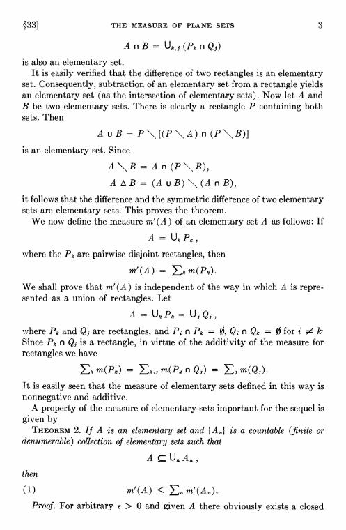
A property of the measure of elementary sets important for the sequel isgiven by
THEOREM 2. If A is an elementary set and { A is a countable (finite ordenumerable) collection of elementary sets such that
A
then
(1) m'(A) <Proof. For arbitrary 0 and given A there obviously exists a closed

4 MEASURE THEORY [cm v
elementary set A contained in A and satisfying the condition
m'(A) � m'(A) — e/2.
[It is sufficient to replace each of the k rectangles whose union is A by aclosed rectangle contained in P1 and having an area greater than —
/ k+1
Furthermore, for each n there is an open elementary set containingand such that
< +It is clear that
A
Since A is compact, by the Heine-Borel theorem (see §18, Theorem 4)contains a finite subsequence ••• , which covers A. Ob-
viously,
m'(A) �[In the contrary case A would be covered by a finite number of rectanglesthe sum of whose areas is less than m' (A), which is clearly impossible.]Therefore,
m'(A) � m'(A) + €/2 < + €/2
� + €/2
+ €/2
= + €.
Since 0 is arbitrary, (1) follows.The class of elementary sets does not exhaust all the sets considered in
elementary geometry and classical analysis. It is therefore natural to posethe question of extending the concept of measure, while retaining itsfundamental properties, to a class of sets wider than the finite unions ofrectangles with sides parallel to the coordinate axes.
This problem was solved, in a certain sense definitively, by Lebesgue inthe early years of the twentieth century.
In presenting the Lebesgue theory of measure it will be necessary toconsider not only finite, but also infinite unions of rectangles.
In order to avoid infinite values of the measure, we restrict ourselves inthe sequel to sets contained in the square E = {O x 1; 0 � y ç i}.
We define two functions, /1*(A) and on the class of all sets Acontained in E.

§33] THE MEASURE OF PLANE SETS
DEFINITION 1. The outer measure of a set A is
= c UPk},
where the lower bound is taken over all coverings of A by countable collectionsof rectangles.
DEFINITION 2. The inner measure of a set A is
= 1 —
It is easy to see that
/.L*(A) �
for every set A.For, suppose that there is a set A C E such that
>
/1*(A) <1.Then there exist sets of rectangles and covering A and E \ A,respectively, such that
+ <1.Denoting the union of the sets and {Qk} by {R5}, we see that
E ç U,R,, m(E)>This contradicts Theorem 2.
DEFINITION 3. A set A is said to be measurable (in the sense of Lebesgue)if
=
The common value /1(A) of the outer and inner measures of a measurableset A is called its Lebesgue measure.
We shall derive the fundamental properties of Lebesgue measure andmeasurable sets, but first we prove the following property of outer measure.
THEOREM 3. If
A
where{ is a countable collection of sets, then
/1*(A) �
Proof. According to the definition of outer measure, for each n and every

MEASURE THEORY {CH. V
0 there is a countable collection of rectangles such that
A
and
/1*(A) � Ekm(Pflk) � +This completes the proof of the theorem.
Theorem 4 below shows that the measure m' introduced for elementarysets coincides with the Lebesgue measure of such sets.
THEOREM 4. Every elementary set A is measurable, and /1(A) = m' (A).Proof. If A is an elementary set and P1, ••• , are rectangles whose
union is A, then by definition
m'(A) =
Since the rectangles cover A,
/1*(A) � = m'(A).
But if is an arbitrary countable set of rectangles covering A, then, byTheorem 2, m'(A) � m(Q,). Consequently, m'(A) � /1*(A). Hence,m'(A) =
Since E \ A is also an elementary set, m'(E \ A) = /1*(E\ A). But
m'(E\A) = 1 — m'(A), = 1 —
Hence,
m'(A) =
Therefore,
m'(A) = = /1*(A) = /1(A).
Theorem 4 implies that Theorem 2 is a special case of Theorem 3.THEOREM 5. In order that a set A be measurable it is necessary and sufficient
that it have the following property: for every 0 there exists an elementaryset B such that
/1*(A <€.In other words, the measurable sets are precisely those which can be
approximated to an arbitrary degree of accuracy by elementary sets. Forthe proof of Theorem 5 we require the following

§33] THE MEASURE OF PLANE SETS 7
LEMMA. For arbitrary sets A and B,
— � B).
Proof of the Lemma. Since
Ac B U (Ait follows that
� +Hence the lemma follows if � < the lemmafollows from the inequality
� +which is proved in the same way as the inequality above.
Proof of Theorem 5.Sufficiency. Suppose that for arbitrary e > 0 there exists an elementary
set B such that,1*(A <e.
Then, according to the Lemma,
(1) — m'(B)I
= —
In the same way, since
(E\A) (E\B) = A
it follows that
(2) — m'(E\B)I <e.Inequalities (1) and (2) and
m'(B) + m'(E\B) = m'(E)
imply that
+!.L*(E\A) — ii <2€.
Since 0 is arbitrary,
+ !1*(E\A) = 1,
and the set A is measurable.Necessity. Suppose that A is measurable, i.e.,
+ = 1.
For arbitrary 0 there exist sets of rectangles and { such that

8 MEASURE THEORY [cii. V
and such that
� + €/3, � + €/3.Since < there is an N such that
< €/3;
set
B=It is clear that the set
P =contains A \ B, while the set
Q = (B n
contains B \ A. Consequently, A B P u Q. Also
� <€/3.Let us estimate /1*(Q). To this end, we note that
u =
and consequently
(3) + � 1.But, by hypothesis,
+ � + + 2€/3
=1+2€/3.From (3) and (4) we obtain
— \ B) = n B) < 2€/3,
< 2€/3.
Therefore,
B) < + !1*(Q) < E
Hence, if A is measurable, for every 0 there exists an elementary set Bsuch that ,L*(A B) < €. This proves Theorem 5.

§33] THE MEASURE OF PLANE SETS 9
THEOREM 6. The union and intersection of a finite number of measurablesets are measurable sets.
Proof. It is clearly enough to prove the assertion for two sets. Supposethat A1 and A2 are measurable sets. Then for arbitrary 0 there areelementary sets B1 and B2 such that
B1) < €/2, B2) < €/2.
Since
(A1 u A2) (B1 u B2) c (A1 B1) u (A2 B2),
it follows that
(5) u A2) (B1 U B2)] � B1) + !1*(A2 B2) <
Since B1 U B2 is an elementary set, it follows from Theorem 4 that A1 u A2is measurable.
But in view of the definition of measurable set, if A is measurable, so isE \ A; hence, A1 n A2 is measurable because of the relation
A1 n A2 = E\ {(E\ A1) u (E \ A2)].
COROLLARY. The difference and symmetric difference of two measurablesets are measurable.
This follows from Theorem 6 and the relations
A1\A2 = A1n (E\A2),
A1 = (A1\A2) u (A2\A1).THEOREM 7. If A1, , are pairwise disjoint measurable sets, then
=
Proof. As in Theorem 6, it is sufficient to consider the case n = 2. Choosean arbitrary 0 and elementary sets B1 and B2 such that
(6) B1) < €,
(7) B2) < €.
Set A = A1 u A2 and B = B1 u B2. According to Theorem 6, the set Ais measurable. Since
B1nB2 u
(8) m'(B1 n B2) � 2€.
In virtue of the Lemma to Theorem 5, (6) and (7) imply that
(9)1
—I

10 MEASURE THEORY [cH. V
(10) m'(B2) —I
<€.
Since the measure is additive on the class of elementary sets, (8), (9) and(10) yield
m'(B) = m'(B1) + m'(B2) — m'(B1 n B2) � + !.L*(A2) — 4€.
Noting that A B (A1 B1) u (A2 B2), we finally have
� m'(B) � m'(B) — 2€ � + !.L*(A2) — 6€.
Since 6€ may be chosen arbitrarily small,
� + !1*(A2).
Inasmuch as the converse inequality
< + !1*(A2)
is always true for A = A1 u A2, we have
= +Since A1 , A2 and A are measurable, can be replaced by /1, and this provesthe theorem.
THEOREM 8. The union and intersection of a countable number of measur-able sets are measurable sets.
Proof. Let
A1 . • , ,
be a countable collection of measurable sets, and let A =A that the sets
are pairwise disjoint. By Theorem 6 and its Corollary, all the sets aremeasurable. According to Theorems 7 and 3,
= ç
for arbitrary finite n. Therefore, the series
converges, and consequently for arbitrary 0 there exists an N such that
(11) < €/2.
Since the set C = is measurable (as a union of a finite number ofmeasurable sets), there exists an elementary set B such that
(12) B) < €/2.
Inasmuch as
A ç (CAB) u (Ufl>NAfl'),
§33] THE MEASURE OF PLANE SETS 11
(11) and (12) imply that
B) <€.Hence, by Theorem 5, the set A is measurable.
Since the complement of a measurable set is measurable, the second halfof the theorem follows from the relation
=
Theorem 8 is a generalization of Theorem 6. The following theorem is thecorresponding generalization of Theorem 7.
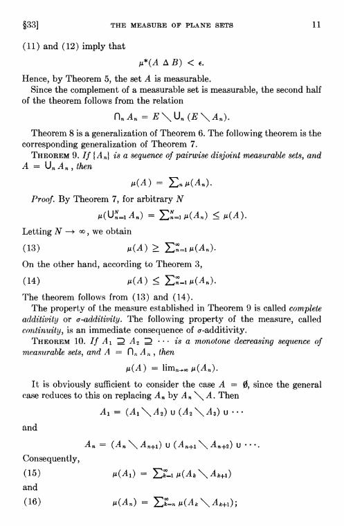
THEOREM 9. If { is a sequence of pairwise disjoint measurable sets, andA =
=
Proof. By Theorem 7, for arbitrary N
= �Letting N —÷ we obtain
(13) ,1(A) �On the other hand, according to Theorem 3,
(14) �The theorem follows from (13) and (14).
The property of the measure established in Theorem 9 is called completeadditivity or cr-additivity. The following property of the measure, calledcontinuity, is an immediate consequence of cr-additivity.
THEOREM 10. If A1 A2 is a monotone decreasing sequence ofmeasurable sets, and A = A , then
=
It is obviously sufficient to consider the case A = 0, since the generalcase reduces to this on replacing by \ A. Then
A1 = (A1\A2) u (A2\A3) uand
= u u
Consequently,
(15) =and
(16) = ,u(Ak\Ak+l);
MEASURE THEORY [OH. V
since the series (15) converges, its remainder (16) approaches zero asn —÷ Hence,
This is what we were to prove.COROLLARY. If A1 A2 is a monotone increasing sequence of meas-
urable sets and A = then
/2(A) =
To prove this it is sufficient to replace the sets by their complementsand then to use Theorem 10.
We have now extended the measure defined on the elementary sets tothe wider class of measurable sets. The latter class is closed with respectto the operations of countable unions and intersections, and the measureon this class is a--additive.
We conclude this section with a few remarks.1. The theorems we have proved characterize the class of Lebesgue
measurable sets.Since every open set contained in E can be written as a union of a count-
able number of open rectangles, that is, measurable sets, Theorem 8 im-plies that every open set is measurable. The closed sets are also measurable,since they are the complements of the open sets. In view of Theorem 8, allsets which can be obtained from the open and closed sets by taking count-able unions and intersections are also measurable. It can be shown, how-ever, that these sets do not exhaust the class of all Lebesgue measurablesets.
2. We have considered only plane sets contained in the unit squareE = {0 x, y 11. It is not hard to remove this restriction. This can bedone, for instance, in the following way. Representing the whole plane asthe union of the squares Enm = {n � x n + 1, m < y < m + 1 (m, nintegers) ,we define a plane set A to be measurable if its intersection AA ii Enm with each of these squares is measurable, and the series
/2(Anm)
converges. We then define
M(Anm).
All the measure properties derived above carry over in an obvious fashionto this case.
3. In this section we have constructed Lebesgue measure for plane sets.Lebesgue measure on the line, in three dimensions, or, in general, in Eucli-dean n-space, can be constructed analogously. The measure in all these

§33] THE MEASURE OF PLANE SETS 13
cases is constructed in the same way: starting with a measure defined fora certain class of simple sets (rectangles in the plane; open, closed andhalf-open intervals on the line; etc.) we first define a measure for finiteunions of such sets, and then extend it to the much wider class of Lebesguemeasurable sets. The definition of measurable set is carried over verbatimto sets in a space of arbitrary (finite) dimension.
4. To introduce Lebesgue measure we started with the usual definitionof area. The analogous construction in one dimension is based on the lengthof an interval. However, the concept of measure can be introduced in an-other, somewhat more general, way.
Let F(t) be a nondecreasing and left continuous function defined on thereal line. We set
m(a, b) = F(b) — F(a + 0),m[a, b] = F(b + 0) —
m(a, b] = F(b + 0) — F(a + 0),m[a, b) = F(b) — F(a).
It is easily verified that the interval function m defined in this way is non-negative and additive. Proceeding in the same way as described above,we can construct a certain "measure" /2p(A). The class of sets measurablerelative to this measure is closed under the operations of countable unionsand intersections, and /2F is cr-additive. The class of MF-measurable sets will,in general, depend on the choice of the function F. However, the open andclosed sets, and consequently their countable unions and intersections,will be measurable for arbitrary choice of F. The measures where Fis arbitrary (except for the conditions imposed above), are called Lebesgue-Stieltjes measures. In particular, the function F(t) t corresponds to theusual Lebesgue measure on the real line.
A measure /2F which is equal to zero on every set whose Lebesgue meas-ure is zero is said to be absolutely continuous. A measure /2F whose set ofvalues is countable [this will occur whenever the set of values of F(t) iscountable] is said to be discrete. A measure /2F is called singular if it is zeroon every set consisting of one point, and if there is a set M whose Lebesguemeasure is zero and such that the /2F measure of its complement is zero.
It can be proved that every measure is a sum of an absolutely con-tinuous, a discrete and a singular measure.
* Existence of nonmeasurable sets. We proved above that the class ofLebesgue measurable sets is very wide. The question naturally ariseswhether there exist nonmeasurable sets. We shall prove that there are suchsets. The simplest example of a nonmeasurable set can be constructed ona circumference.
14 MEASURE THEORY [OH. V
Let C be a circumference of length 1, and let a be an irrational number.Partition the points of C into classes by the following rule: Two points ofC belong to the same class if, and only if, one can be carried into the otherby a rotation of C through an angle na (n an integer). Each class is clearlycountable. We now select a point from each class. We show that the re-sulting set is nonmeasurable. Denote by the set obtained by rotating
through the angle na. It is easily seen that all the sets are pairwisedisjoint and that their union is C. If the set were measurable, the sets
congruent to it would also be measurable. Since
C = = 0 (n m),
the o--additivity of the measure would imply that
(17) = 1.
But congruent sets must have the same measure:
=
The last equality shows that (17) is impossible, since the sum of the serieson the left side of (17) is zero if = 0, and is infinity if > 0.Hence, the set (and consequently every set is nonmeasurable. *
EXERCISES
1. If A is a countable set of points contained in
E = {(x, y):0 x � 1,0 � y � 11,
then A is measurable and /2(A) = 0.2. Let F0 = [0, 1] and let F be the Cantor set constructed on F0 (see
vol. 1, pp. 32—33). Prove that /21(F) = 0, where jii(F) is the (linear)Lebesgue measure of F.
3. Let F be as in Ex. 2. If x E F, then
x = ai/3 + + +where a1 = 0 or 2. Define
cc(x) = ai/22 + + + (x E F)
(see the reference given in Ex. 2). The function cc is single-valued. If a,b E F are such that (a, b) F [i.e., (a, b) is a deleted open interval in theconstruction of F], show that p(a) = p(b). We can therefore define cc on[a, b] as equal to this common value. The function cc so defined on F0 =[0, 1] is nondecreasing and continuous. Show that , the Lebesgue-Stieltjesmeasure generated by cc on the set F0, is a singular measure. The functioncc is called the Cantor function.
§34] COLLECTIONS OF SETS 15
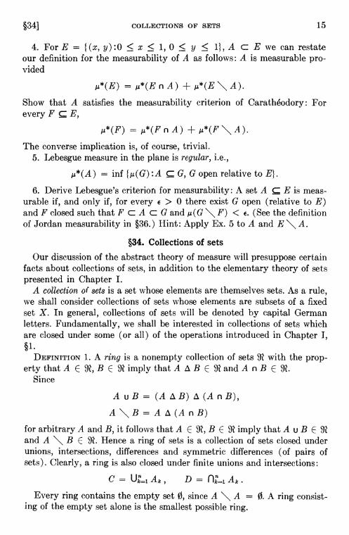
4. For E = { (x, y) :0 x � 1, 0 � y 1}, A C E we can restateour definition for the measurability of A as follows: A is measurable pro-vided
= /1*(EflA)
Show that A satisfies the measurability criterion of Carathéodory: Forevery F
= n A) + M*(F \ A).
The converse implication is, of course, trivial.5. Lebesgue measure in the plane is regular, i.e.,
12*(A) = inf :A G, G open relative to E}.
6. Derive Lebesgue's criterion for measurability: A set A E is meas-urable if, and only if, for every 0 there exist G open (relative to B)and F closed such that F C A C G and /2(G \ F) < €. (See the definitionof Jordan measurability in §36.) Hint: Apply Ex. 5 to A and E \ A.
§34. Collections of sets
Our discussion of the abstract theory of measure will presuppose certainfacts about collections of sets, in addition to the elementary theory of setspresented in Chapter I.
A collection of sets is a set whose elements are themselves sets. As a rule,we shall consider collections of sets whose elements are subsets of a fixedset X. In general, collections of sets will be denoted by capital Germanletters. Fundamentally, we shall be interested in collections of sets whichare closed under some (or all) of the operations introduced in Chapter 1,§1.
DEFINITION 1. A ring is a nonempty collection of sets with the prop-erty that A E B E imply that A B E and A ii B E
Since
AuB=(A nB)
A A Aand B E Hence a ring of sets is a collection of sets closed underunions, intersections, differences and symmetric differences (of pairs ofsets). Clearly, a ring is also closed under finite unions and intersections:
Every ring contains the empty set 0, since A \ A 0. A ring consist-ing of the empty set alone is the smallest possible ring.

16 MEASURE THEORY [cH. V
A set B is called a unit of a collection of sets if it is an element ofand if
AnE=Afor arbitrary A E It is easily seen that if has a unit, it is unique.
Hence, the unit of a collection of sets is the maximal set of the collec-tion, that is, the set which contains every other element of
A ring of sets with a unit is called an algebra of sets. [TRANS. NOTE. Thisdefinition leads to difficulties in the statements and proofs of certain the-orems in the sequel. These difficulties disappear if the usual definition ofan algebra is used: Let X be a set, a collection of subsets of X. The col-lection is called an algebra if is a ring with unit E = X.J
EXAMPLES. 1. If A is an arbitrary set, the collection of all its sub-sets is an algebra of sets with unit E = A.
2. If A is an arbitrary nonempty set, the collection {ø, A} consisting ofthe set A and the empty set 0 is an algebra with unit E A.
3. The set of all finite subsets of an arbitrary set A is a ring. This ringis an algebra if, and only, if A is finite.
4. The set of all bounded subsets of the real line is a ring without a unit.An immediate consequence of the definition of a ring isTHEOREM 1. The intersection = fl a a of an arbitrary number of rings
is a ring.We shall prove the following simple, but important, proposition:THEOREM 2. If is an arbitrary nonempty collection of sets, there exists
precisely one ring ( containing and contained in every ring contain-ing
Proof. It is easy to see that the ring is uniquely determined byTo show that it exists, we consider the union X = UA E A and the ring
of all the subsets of X. Let be the collection of all rings containedin and containing The intersection
=
is obviously the required ringFor, if is a ring containing then = n is a ring in
hence,
that is, is minimal. ( is called the minimal ring over the collectionis also called the ring generated by
The actual construction of the ring over a prescribed collectionis, in general, quite complicated. However, it becomes completely explicitin the important special case when is a semi-ring.
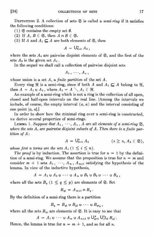
§34] COLLECTIONS OF SETS 17
DEFINITION 2. A collection of sets is called a semi-ring if it satisfiesthe following conditions:
(1) contains the empty set 0.(2) If A, BE then A nB E(3) If A and A1 A are both elements of then
A =
where the sets Ak are pairwise disjoint elements of and the first of thesets Ak is the given set A1.
In the sequel we shall call a collection of pairwise disjoint sets
A1 , • ,
whose union is a set A, a finite partition of the set A.Every ring is a semi-ring, since if both A and A1 A belong to
then A = A1 u A2, where A2 = A \ A1 E
An example of a semi-ring which is not a ring is the collection of all open,closed and half-open intervals on the real line. [Among the intervals weinclude, of course, the empty interval (a, a) and the interval consisting ofone point [a, a].]
In order to show how the minimal ring over a semi-ring is constructed,we derive several properties of semi-rings.
LEMMA 1. Suppose that A1, •••, A are all elements of a semi-ringwhere the sets are pairwise disjoint subsets of A. Then there is a finite par-tition of A:
A = (s � n, Ak Ewhose first n terms are the sets (1 $ i n).
The proof is by induction. The assertion is true for n = 1 by the defini-tion of a semi-ring. We assume that the proposition is true for n = m andconsider m + 1 sets A1, Am, satisfying the hypothesis of thelemma. In view of the inductive hypothesis,
where all the sets (1 � q � p) are elements of Set
= Am+i n Bq.
By the definition of a semi-ring there is a partition
U U U Bqrq,
where all the sets are elements of It is easy to see thatA = A1 U U Am U Am+i U Be,.
Hence, the lemma is true for n = m + 1, and so for all n.
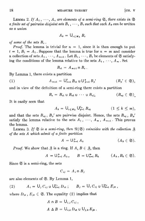
18 MEASURE THEORY [OH. V
LEMMA 2. If A1, •.•, are elements of a semi-ring there exists ina finite set of pairwise disjoint sets B1, • •, Bt such that each Ak can be writtenas a union
Ak U8EMk B.
of some of the sets B8.Proof. The lemma is trivial for n = 1, since it is then enough to put= 1, B1 A1. Suppose that the lemma is true for n = m and consider
a collection of sets A1, , A m+1. Let B1, •••, be elements of satisfy-ing the conditions of the lemma relative to the sets A1, Am. Set
B81 = Am+i B8.
By Lemma 1, there exists a partition
(1) = U (Br' E
and in view of the definition of a semi-ring there exists a partition
B3 = B81 U B82 U U B818 (B8q E
It is easily seen that
and that the sets are pairwise disjoint. Hence, the sets Bsq,satisfy the lemma relative to the sets A1, .. •, Am, A m+1 . This provesthe lemma.
LEMMA 3. If is a semi-ring, then coincides with the collectionof the sets A which admit of a finite partition
A = (Ak E
Proof. We show that is a ring. If A, B E (3,then
Since is a semi-ring, the sets
= A. n B
are also elements of By Lemma 1,
(2) = U u D2k ; B1 = u EJk,
where D2k, E The equality (2) implies that
A n B =
A U1,kD1k u UJ,kEJk.
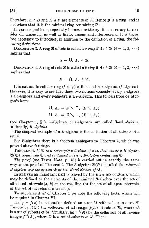
§34] COLLECTIONS OF SETS 19
Therefore, A ii B and A B are elements of 2. Hence is a ring, and itis obvious that it is the minimal ring containing
In various problems, especially in measure theory, it is necessary to con-sider denumerable, as well as finite, unions and intersections. It is there-fore necessary to introduce, in addition to the definition of a ring, the fol-lowing definitions.
DEFINITION 3. A ring of sets is called a o-ring if A2 E (i = 1, 2,implies that
S = Un
A ring of sets is called a s-ring if A E (i = 1, 2,implies that
D = ft, E
It is natural to call a cr-ring (s-ring) with a unit a a-algebra (s-algebra).However, it is easy to see that these two notions coincide: every cr-algebrais a s-algebra and every s-algebra is a cr-algebra. This follows from de Mor-gan's laws:
UflAfl E\ (E\Afl),flflAfl = E\
(see Chapter 1, §1). cr-algebras, or s-algebras, are called Borel algebras;or, briefly, B-algebras.
The simplest example of a B-algebra is the collection of all subsets of aset A.
For B-algebras there is a theorem analogous to Theorem 2, which wasproved above for rings.
THEOREM 4. If is a nonempty collection of sets, there exists a B-algebracontaining and contained in every B-algebra containing
The proof (see Trans. Note, p. 16) is carried out in exactly the sameway as the proof of Theorem 2. The B-algebra is called the minimalB-algebra over the system or the Borel closure of
In analysis an important part is played by the Borel sets or B-sets, whichmay be defined as the elements of the minimal B-algebra over the set ofall closed intervals [a, b] on the real line (or the set of all open intervals,or the set of half-closed intervals).
To supplement §7 of Chapter 1 we note the following facts, which willbe required in Chapter VI.
Let y = f(x) be a function defined on a set M with values in a set N.Denote by the collection of all images f(A) of sets in whereis a set of subsets of M. Similarly, let be the collection of all inverseimages f'(A), where is a set of subsets of N. Then:
20 MEASURE THEORY [OH. V
1. If is a ring, is a ring.2. If is an algebra, is an algebra.3. If is a B-algebra, is a B-algebra.4.5.
* Let be a ring of sets. If the operations A B and A n B are regardedas addition and multiplication, respectively, then is a ring in the usualalgebraic sense. All its elements satisfy the conditions
(*) a+a==O, a2=a.A ring all of whose elements satisfy the conditions (*) is called a Booleanring. Every Boolean ring can be realized as a ring of sets with the opera-tions A B and A ii B (Stone). *
EXERCISES
1. Suppose that is a ring of subsets of a set X and that is the col-lection of those sets E ç X for which either E E or else X \ E E
Show that is an algebra with unit X.2. Determine the minimal ring in each of the following cases:(a) for a fixed subset A ç X, = {A1;(b) for a fixed subset A ç X, = {B:A ç B ç X}.3. Let be a semi-ring in X, and let be the minimal ring overThen the minimal cr-rings over and coincide.
4. For each of the following sets what are the cr-ring and the Borel alge-bra generated by the given class of sets
(a) Let T be a one-to-one onto transformation of X with itself. A sub—set A X is called invariant if x E A implies that T(x) E A and T'(x)E A. Let be the collection of invariant subsets of X.
(b) Let X be the plane and let be the collection of all subsets of theplane which can be covered by countably many horizontal lines.
§35. Measures on semi-rings. Extension of a measure on a semi-ring tothe minimal ring over the semi-ring
In §33, to define a measure in the plane we started with the measure(area) of rectangles and then extended this measure to a more generalclass of sets. The results and methods of §33 are completely general andcan be extended, with no essential changes, to measures defined on ar-bitrary sets. The first step in the construction of a measure in the planeis the extension of the measure of rectangles to elementary sets, that is, tofinite unions of pairwise disjoint rectangles.
We consider the abstract analogue of this problem in this section.DEFINITION 1. A set function /1(A) is called a measure if
§35] MEASURES ON SEMI-RINGS 21
1) its domain of definition is a semi-ring;2) its values are real and nonnegative;3) it is additive, that is, if
A = Uk A,,
is a finite partition of a set A E in sets A,, E then
/1(A) =
REMARK. Since 0 = 0 u 0, it follows that = 2/1(0), i.e., ii(O) = 0.The following two theorems on measures in semi-rings will be applied
repeatedly in the sequel.THEOREM 1. Let be a measure defined on a semi-ring If
A1, • •, A E
where the sets Ak are pairwise disjoint subsets of A, then
�/1(A).Proof. Since is a semi-ring, in view of Lemma 1 of §34 there exists a
partition
A = (s � n, Ak E
in which the first n sets coincide with the given sets A1, An.. Sincethe measure of an arbitrary set is nonnegative,
Ek=l/1(Ak) � Ek=l/1(Ak) = /1(A).
THEOREM 2. If A1, •••, A A Ak, then
/1(A) Ek=l/1(Ak).
Proof. According to Lemma 2 of §34 there exist pairwise disjoint setsB1, ..., E S,. such that each of the sets A, A1, •.., can be writtenas a union of some of the sets B3
A U3 EM0 B3; Ak = USEMk B3 (1 � k � n)where each index s E M0 is an element of some Mk. Consequently, everyterm of the sum
ESEMO /l(B3) =
appears at least once in the double sum
ESEMk /2(B3) =
Hence,
/2(A)

22 MEASURE THEORY [cii. v
In particular, if n = 1, we obtain theCOROLLARY. If A A', then ,u(A)DEFINITION 2. A measure /2(A) is said to be an extension of a measure
m(A) if Sm and if ,u(A) m(A) for every A E Sm.The primary purpose of this section is to prove the following theorem.THEOREM 3. Every measure m(A) has a unique extension /1 whose
domain of definition is the ring Sm).Proof. For each set A E there exists a partition
(1) A = Bk (Bk E Sm)
(§34, Theorem 3). We set, by definition,
(2) m(Bk).
It is easily seen that the value of /2(A) defined by (2) is independent ofthe choice of the partition (1). In fact, let
A_Urn — n / I—i=1 i 5=1 j i m , 5 m
be two partitions of A. Since all the intersections n C5 belong to Sm,in view of the additivity of the measure m,
m(B1) = n = m(C5).
The measure 12(A) defined by (2) is obviously nonnegative and additive.This proves the existence of an extension /1(A) of the measure m. To proveits uniqueness, we note that, according to the definition of an extension,if A = Bk, where the Bk are disjoint elements of Sm, then
= E/1*(B/) = Em(Bk) = /1(A)
for an arbitrary extension /2* of m over This proves the theorem.The relation of this theorem to the constructions of §33 will be fully
clear if we note that the set of all rectangles in the plane is a semi-ring,that the area of the rectangles is a measure in the sense of Def. 1 and thatthe class of elementary plane sets is the minimal ring over the semi-ringof rectangles.
EXERCISES
1. Let X be the set of positive integers, the set of all finite subsets ofX. Suppose that is a convergent series of positive numbers. ForA E define p (A) = u. (n E A). Prove that ji is a measure. Nowsuppose that is the set of all subsets of X and that is defined as abovefor finite subsets of X, but that /2(A) = + if A is infinite. is still fi-nitely additive [although ji(A) may equal + for some sets]. How-ever, is not completely additive (see §37, Def. 1).

§36] EXTENSION OF JORDAN MEASURE 23
2 Let X be the plane, and let = {A : A = the set of all (x, y) suchthat a < x b, y = c}, i.e., consists of all the horizontal right half-closed line segments. Define /2(A) = b — a.
(a) Show that is a semi-ring.(b) Show that /L is a measure on
3. Let /1 be a measure on a ring(a) For A, B E show that /2(A u B) + — /2(A n B).(b) For A, B, C E show that
u B u C) = + +— [,u(A n B) + 12(B fl C) + ,u(C n A)] + /2(A n B n C),
(c) Generalize to the case A1, •••, E
§36. Extension of the Jordan measure
The concept of Jordan measure is of historical and practical interest,but will not be used in the sequel.
In this section we shall consider the general form of the process whichin the case of plane figures is used to pass from the definition of the areasof finite unions of rectangles with sides parallel to the coordinate axes tothe areas of those figures which are assigned definite areas in elementarygeometry or classical analysis. This transition was described with com-plete clarity by the French mathematician Jordan about 1880. Jordan'sbasic idea, however, goes back to the mathematicians of ancient Greeceand consists in approximating the "measurable" sets A by sets A' and A"such that
A' ç A ç A".
Since an arbitrary measure can be extended to a ring (§35, Theorem 3),it is natural to assume that the initial measure m is defined on the ring
= Sm). We shall make this assumption in the rest of this section.DEFINITION 1. We shall say that a set A is Jordan measurable if for every> 0 there are sets A', A" E such that
A' A A", m(A" \ A') <€.
THEOREM 1. The collection of sets which are Jordan measurable is aring.
For, suppose that A, B E then for arbitrary 0 there exist setsA', A", B', B" E such that
A'çAçA", B'çBçB"

24 MEASURE THEORY [cH. V
and
m(A" \ A') < m(B" \ B') <
Hence
(1)
(2)
Since
(A" u B") \ (A' u B') (A" \ A') u (B" \ B'),
m[(A" u B") \ (A' u B')] <m[(A" \ A') u (B" \ B')]
<m(A" \ A') + m(B" \ B')
< + =
Since
(A" \ B') \ (A' \ B") (A" \ A') u (B" \ B'),
m[(A" \ B') \ (A' \ B")] <m(A" \ A') u (B" \ B')](4)
<m(A"\A') + m(B11\B')< + E/2 =
Inasmuch as > 0 is arbitrary and the sets A' u B', A" u B", A' \ B",A" \ B' are elements of (1), (2), (3) and (4) imply that A u B andA \ B are elements of
Let be the collection consisting of the sets A for which there is a setB E such that B A. For arbitrary A E we define
= inf{m(B);BM(A) = sup {m(B); B A}.
The functions jz(A) and M(A) are called the outer and inner measures,respectively, of the set A.
Obviously,
THEOREM 2. The ring coincides with the system of all sets A E suchthatM(A) =
Proof. If
M(A),
then

EXTENSION OF JORDAN MEASURE 25
— M(A) = h > 0,
and
m(A') m(A") > ji(A),
m(A"\A') = m(A") — m(A') � h >0for arbitrary A', A" E such that A' A A". Hence A
Conversely, if
M(A)
then for arbitrary > 0 there exist A', A" E such that
A' A A",
M(A) — m(A') <
m(A") — ji(A) <€/2,
m(A" \ A') m(A") — m(A') <€,i.e., A E
The following theorem holds for sets ofTHEOREM 3. If A Ak, then �Proof. Choose an Ak' such that
Ak Ak', m(Ak') � + 6/2k,
and let A' U Ak'. Then
m(A') � � + €,
,i(A) � ,ü(Ak) +since is arbitrary, �
THEOREM 4. If Ak A (1 � k � n) and A n A ç 0, then
M(A) � M(Aic).
Proof. Choose Ak' such that m(Ak') � — 12k and letA' = Ak'. Then A/ n A5' 0 and
m(A') = � —
Since A' A, M(A) � m(A') � — Since > 0 is ar-bitrary, M(A) � M(Ak).
We now define the function /1 with domain of definition

26 MEASURE THEORY
as the common value of the inner and outer measures:
= M(A) =
Theorems 3 and 4 and the obvious fact that
= = m(A) (A E
implyTHEOREM 5. The function /2(A) is a measure and is an of the
measure m.The construction we have discussed above is applicable to an arbitrary
measure m defined on a ring.The collection Sm2 = of elementary sets in the p'ane is essentially
connected with the coordinate system: the sets of the collection consistof the rectangles whose sides are parallel to the coordinate axes. In thetransition to the Jordan measure
(2)Jthis dependence on the choice of the coordinate system vanishes: if {is a system of coordinates related to the original coordinate system {x1, x21
by the orthogonal transformation
xi cos a + x2 sin a + a1,
—x1 sin a + x2 cos a + a2,
we obtain the same Jordan measurej(2) = j(m2) =
where denotes the measure constructed by means of rectangles withsides parallel to the axes This fact is justified by the following gen-eral theorem:
THEOREM 6. In order that two Jordan extensions /11 = j(m1) and /22 =j(m2) of measures m1 and m2 defined on rings and coincide, it is neces-sary and sufficient that
m1(A) = /22(A) on
m2(A) /21(A) on
The necessity is obvious. We shall prove the sufficiency.Suppose that A E . Then there exist A', A" E such that
A' A A", m1(A") — m1(A') <
and mi(A') � � mi(A"). By hypothesis, 1i2(A') = m1(A') and= mi(A").

§36] EXTENSION OF JORDAN MEASURE 27
In view of the definition of the measure there exist sets B', B" Esuch that
A' D B', — m2(B') < €/3;
B" A", m2(B") — < €/3.
Hence
B' ç A B",
and, obviously,
m2(B") — m2(B')
Since 0 is arbitrary, A E ; and the relations
/li(B') = in2(B') < < in2(B") =
imply that /12 is an extension of Mi. Similarly, one shows that is an ex-tension of M2, and therefore
p2(A) — p1(A).
rfhis proves the theorem.Now, to show the independence of the ,Jordan measure in the plane of
the choice of the coordinate system we need merely show that the set ob-tained from an elementary set by a rotation through an angle a is Jordanmeasurable. It is left to the reader to carry out this proof.
If the original measure m is defined on a semi-ring instead of a ring, itis natural to call the measure
j(m) = j(r(m))obtained by extending m over the ring Sm) and then extending thelatter to a Jordan measure, the Jordan extension of m.
EXERCISES
1. If AB is a line segment in the plane, then = 0.
2. Let ABC be a right triangle in the plane, with AB perpendicular toBC and with AB and BC parallel to the x- and y-axes, respectively.
a) Show that ABC isb) Using the invariance of j(2) under translation and reflection in an
axis, show that j(2) (ABC) = (BC).3. a) It follows from Ex. 2 and the text that any triangle is
urable and that its is the classical area.b) Show, therefore, that a regular polygon is and re-
ceives its classical area.

28 MEASURE THEORY [cH. V
c) It follows now that a circle, i.e., a closed disk, is4. Show that the plane set A = { (x, y) x2 + y2 � 1, x, y rationall is
not j(2) -measurable.
§37. Complete additivity. The general problem of the extension of measures
It is often necessary to consider countable unions as well as finite unions.Therefore, the condition of additivity we imposed on a measure (§34, Def.1) is insufficient, and it is natural to replace it by the stronger conditionof complete additivity.
DEFINITION 1. A measure /L is said to be completely additive (ortive) if A, A1, , , E where is the collection of sets onwhich /L is defined, and
imply that
=
The plane Lebesgue measure constructed in §33 is a-additive (Theorem9). An altogether different example of a a-additive measure may be con-structed in the following way. Let
X={xj,x2,..•1be an arbitrary countable set and let the numbers Pn > 0 be such that
Pn = 1.
The set consists of all the subsets of X. For each A X set
=
It is easy to verify that /2(A) is a a-additive measure and that = 1.
This example appears naturally in many problems in the theory of proba-bility.
We shall also give an example of a measure which is additive, but nota-additive. Let X be the set of all rational points on the closed interval[0, 1] and let SM consist of the intersections of X with arbitrary intervals(a, b), [a, b], [a, b) or (a, bJ. It is easily seen that S,L is a semi-ring. Foreach set Aab E set
/2(Aab) — b — a.
Then /L is an additive measure. It is not a-additive since, for instance,= 1, but X is the union of a countable number of points each of
which has measure zero.In this and the succeeding two sections we shall consider a-additive
measures and their a-additive extensions.
§37] COMPLETE ADDITIVITY. EXTENSION OF MEASURES 29
THEOREM 1. If a measure m defined on a semi-ring Sm is completely addi-tive, then its extension = r(m) to the ring (Sm) is completely additive.
Proof. Suppose that
A E E (n — 1, 2, •..)and that
A =
where B3 n Br = 0 (s r). Then there exist sets A E Sm such that
A = =
where the sets on the right-hand sides of these equalities are pairwise dis-joint and the unions are finite unions Theorem 3).
Let = n A,. It is easy to see that the sets are pairwise dis-joint and that
A,
= U1
Therefore, because of the complete additivity of m on
(1) m(A3) =
(2) =
and because of the definition of r(m) on
(3) /1(A) =
(4) =
Relations (1), (2), (3) and (4) imply that /1(A) = ( Ba). (The sumsover i and j are finite sums, and the series over n converge.)
It could be proved that the Jordan extension of a a-additive measure isa-additive, but it is not necessary to do so because it will follow from thetheory of Lebesgue extensions discussed in the next section.
THEOREM 2. If a measure is a-additive and A, A1, ,
A
implies that
/1(A)
Proof. Because of Theorem 1 it is sufficient to carry out the proof for ameasure defined on a ring, since the validity of Theorem 2 for /L = r(m)immediately implies its applicability to the measure m. If SM is a ring, thesets
30 MEASURE THEORY [OH. v
= (A
are elements of Since
and the sets are pairwise disjoint,
,u(A) <
In the sequel, we shall consider only a-additive measures, without men-tioning this fact explicitly.
* We have considered two ways of extending measures. In extending ameasure m over the ring in §35 we noted the uniqueness of the ex-tension. The same is true for the Jordan extension j(m) of an arbitrarymeasure m. If a set A is Jordan measurable with respect to a measure m(that is, A E Sj(m)), then /1(A) = J(A), where /1 is an arbitrary extensionof m defined on A and J j(m) is the Jordan extension of m. It can beproved that an extension of m to a collection larger than Sj(m) is not unique.More precisely, the following is true. Call a set A a set of unicity for a meas-ure m if
1) there exists an extension of m defined on A;2) for two such extensions pi and P2,
p1(A) = ,12(A).
Then the following theorem holds.The set of sets of unicity of a measure m coincides with the collection
of Jordan measurable sets relative to m, i.e., the collection of sets 85(m)However, if we consider only a-additive measures and their (r-additive)
extensions, then the collection of sets of unicity will, in general, be larger.Since we shall be exclusively occupied with a-additive measures in the
sequel, we introduceDEFINITIoN 2. A set A is said to be a set of for a a-additive
measure /L jf1) there exists a a-additive extension X /1 defined on A (that is, A E Sx);2) if X1, X2 are two such a-additive extensions, then
X1(A) X2(A).
If A is a set of for a a-additive measure p, then the definitionimplies that if there is a a-additive extension X(A) of /1 defined on A, it isunique. *
EXERCISES
1. Suppose is a completely additive measure on the collection of allsubsets of a countable set X. Show that p(A) = 0 for all A X if, and

§38] LEBESGUE EXTENSION OF A MEASURE ON A SEMI-RING 31
only if, /2({x}) = 0 for all x E X, i.e., vanishes on every set consisting ofa single point.
2. If X is a countable set, the class of all subsets of X and a com-pletely additive measure defined on then must necessarily have theform of the second example after Def. 1 in §37, where, however, the Pn needonly satisfy the conditions Pn � 0, Pn <
3. Show that the measure defined in Ex. 2, §35 is completely additive.Hint: Imitate the procedure used in §33, Theorem 2.
4. Let be the semi-ring of left-closed right-open intervals on the line:= { [a, b)}, let F(t) be a nondecreasing left continuous real-valued func-
tion defined on the line and let 12F be the Lebesgue measure defined in Re-mark 4 at the end of §33. Show that is completely additive by followinga procedure analogous to that of Ex. 3 above. It will be necessary to showthe following: Suppose that a < b. For 0 there exist c and d such that
a�c<d<b, [c,d]c[a,b)and
d)) = F(d) — F(c) > F(b) — F(a) — = b)) —
Similarly, there exist e, f such that e < a < b f, [a, b) C (e, f) and= F(f) — F(e) <F(b) — F(a) + E b)) + E.
§38. The Lebesgue extension of a measure defined ona semi-ring with unity
Although the Jordan extension applies to a wide class of sets, it is never-theless inadequate in many cases. Thus, for instance, if we take as the ini-tial measure the area defined on the semi-ring of rectangles and considerthe Jordan extension of this measure, then so comparatively simple a set asthe set of points whose coordinates are rational and satisfy the conditionx2 + y2 < 1 is not Jordan measurable.
The extension of a o-additive measure defined on a semi-ring to a classof sets, which is maximal in a certain sense, can be effected by means of theLebesgue extension. In this section we consider the Lebesgue extension of ameasure defined on a semi-ring with a unit. The general case will be con-sidered in §39.
The construction given below is to a considerable extent a repetition inabstract terms of the construction of the Lebesgue measure for plane setsin §33.
Let m be a i-additive measure defined on a semi-ring Sm with a unit E.We define on the system of all subsets of E the functions /.L*(A) and
as follows.DEFINITIoN 1. The outer measure of a set A ç E is

32 MEASURE THEORY [CII. V
=
where the lower bound is extended over all coverings of A by countable(finite or denumerable) collections of sets E Sm.
DEFINITIoN 2. The inner measure of a set A E is
= m(E) —
Theorem 2 of §35 implies that /.L*(A) �DEFINITION 3. A set A E is said to be (Lebesgue) measurable if
=
If A is measurable, the common value of /.L*(A) = /2*(A) is denoted by12(A) and called the (Lebesgue) measure of A.
Obviously, if A is measurable, its complement E \ A is also measurable.Theorem 2 of §37 immediately implies that
I.L*(A) �
for an arbitrary (i-additive extension of m. Therefore, for a Lebesguemeasurable set A every (i-additive extension /L of m (if it exists) is equal tothe common value of bz*(A) = The Lebesgue measure is thus the(i-additive extension of m to the collection of all sets measurable in thesense of Def. 3. The definition of measurable set can obviously also beformulated as follows:
DEFINITION 3'. A set A E is said to be measurable if
+ = m(E).
It is expedient to use together with the initial measure m its extension= r(m) (see §35) over the ring It is clear that Def. 1 is equiva-
lent toDEFINITIoN 1'. The outer measure of a set A is
= inf { A E [Ba' E
In fact, since m' is (i-additive (§37 rfheorem 1), an arbitrary sumwhere E can be replaced by an equivalent sum
Efl,km(Bflk) (Bflk E Sm),
where
= UkBflk, = 0 (i
The following is fundamental for the sequel.THEOREM 1. If
A

§38] LEBESGUE EXTENSION OF A MEASURE ON A SEMI-RING 33
where { is a countable collection of sets then,
<
E then /.L*(A) = m'(A) = 12*(A), i.e., all the setsof Sm) are measurable and their outer and inner measures coincide with m'.
THEOREM 3. A set A is measurable if, and only if, for arbitrary 0there exists a set B E (Sm) such that
B) <€.These propositions were proved in §33 for plane Lebesgue measure (§33,
Theorems 3—5). The proofs given there carry over verbatim to the generalcase considered here, and so we shall not repeat them.
THEOREM 4. The collection of all measurable sets is a ring.Proof. Since
A1nA2 =
A1 u A2 = E\[(E\A1) n (E\A2)],it is sufficient to prove the following. If A1 , A2 E then
A = A1\A2 E
Let A1 and A2 be measurable; then there exist B1, B2 E such that
B1) < €/2, B2) < E/2.
Setting B = B1 \ B2 E Sm) and using the relation
(A1 \ A2) (B1 \ B2) c (A1 B1) u (A2 B2),
we obtain
B) <€.Hence, A is measurable.
REMARK. It is obvious that E is the unit of the ring so that the latteran algebra.THEOREM 5. 'IThe function /h(A) is additive on the set of measurable
sets.The proof of this theorem is a verbatim repetition of the proof of Theorem
7, §33.THEOREM 6. The function is a-additive on the set of measurable
sets.Proof. Let
A = E A1nA, = 0 if i
By Theorem 1,
34 MEASURE THEORY [CII. V
(1)
and by Theorem 5, for arbitrary N,
�Hence,
(2) �The theorem follows from (1) and (2).
We have therefore proved that the function bz(A) defined on possessesall the properties of a a-additive measure.
This justifies the followingDEFINITION 4. The Lebesgue extension = L(rn) of a measure m(A) is
the function defined on the collection = of measurable setsand coinciding on this collection with the outer measure
In §33, in considering plane Lebesgue measure, we showed that notonly finite, but denumerable unions and intersections of measurable setsare measurable. This is also true in the general case, that is,
THEOREM 7. The collection of Lebesgue measurable sets is a Borel algebrawith unit E.
Proof. Since
and since the complement of a measurable set is measurable, it is sufficientto prove the following: If Ai , A2, , A E
the same as that of Theorem 8, §33, for planesets.
As in the case of plane Lebesgue measure, the i-additivity of the measureimplies its continuity, that is, if is a i-additive measure defined on aB-algebra, and A1 A2 D •.. D D ... is a decreasing sequence ofmeasurable sets, with
A =
then
/2(A)
and if A1 A2 ... C is an increasing sequence of measura-ble sets, with
A =
then

§38] LEBESGUE EXTENSION OF A MEASURE ON A SEMI-RING 35
12(A) =
The proof of this is the same as that of Theorem 10, §33, for plane measure.
* 1. From the results of §37 and §38 we easily conclude that every Jor-dan measurable set A is Lebesgue measurable, and that its Jordan andLebesgue measures are equal. It follows immediately that the Jordan ex-tension of a (i-additive measure is (i-additive.
2. Every Lebesgue measurable set A is a set of unicity for the initialmeasure m. In fact, for arbitrary 0 there exists a set B E such that
B) < €. For every extension X of m defined on A,
X(B) = m'(B),
since the extension of m on = ( is unique. Furthermore,
X(A B) B) <€;consequently,
X(A) — m'(B) <€.Hence,
X1(A) — X2(Afl <2€
for any two extensions X1(A), X2(A) of m. Therefore,
X1(A) = X2(A).
It can be proved that the class of Lebesgue measurable sets includes allthe sets of unicity of an initial measure m.
3. Let m be a (i-additive measure defined on S, and let 9)1 = L(S) bethe domain of definition of its Lebesgue extension. It easily follows fromTheorem 3 of this section that if
S Si
then
L(51) = L(S).*
EXERCISES
1. Show that the collection of subsets A of E for which /2(A) = 0 or\ A) = 0 form a Borel algebra with E as a unit. This algebra is asubalgebra of
2. With the notation of the text for A E let

36 MEASURE THEORY [CII. V
= cA}.Show that =
3. Suppose that A E. Then A E if, and only if, A n B E forall B E Sm.
4. For A E, A E if, and oniy if, for 0 there exist sets B1,B2 E such that B1 c: A C B2 and \ B1) < €. [See §36, Def. 1(Jordan measurability); also compare with §33, Ex. 6.]
5. For any A E we havea)/2*(A)=inf{/2B:ACB,b) ,u*(A) = sup {/LB:B C A, B E
We see therefore that (abstract) Lebesgue measure is (abstractly) regular(see §33, Ex. 5).
6. Let , 5m2 be two semi-rings on X with the same unit E; let m1 , m2be (i-additive measures defined on 5m1 5m2 , respectively; and let p1*, p2*
be the outer measures on the set of all subsets of E defined by using m1 , m2,respectively. Then = p2*(A) for every A E if, and only
= m2(A) for A E 5m2 and p2*(A) = mi(A) for A E Smj. (See§36, Theorem 6 for the analogous theorem on Jordan extensions.)
§39. Extension of Lebesgue measures in the general case
If the semi-ring Sm on which the initial measure m is defined has no unit,the discussion of §38 must be modified. Def. 1 of the outer measure is re-tained, but the outer measure is now defined only on the collectionof the sets A for which there exists a covering of sets of Sm with afinite sum
Def. 2 becomes meaningless. The lower measure can also be defined (inseveral other ways) in the general case, but we shall not do so. It is moreexpedient at this point to define a measurable set in terms of the conditiongiven in Theorem 3.
DEFINITIoN 1. A set A is said to be measurable if for arbitrary 0there exists a set B C such that /2*(A B) <
Theorems 4, 5, 6 and Def. 4 of the preceding section remain true. Theexistence of a unit was used only in the proof of Theorem 4. To reproveTheorem 4 in the general case, it is necessary to show again that A1 , A2 Eimplies that A1 u A2 E The proof of this is carried out in the same wayas for A1 \ A2 on the basis of the relation.
(A1 u A2) (B1 u B2) c (A1 B1) u (A2 B2).
If Sm has no unit, Theorem 7 of §38 changes to
§39] LEBESGIJE EXTENSION IN THE GENERAL CASE 37
THEOREM 1. For arbitrary initial measure m the collection 9)1 = SL(m) ofLebesgue measurable sets is a a set A = , where the setsare measurable, is measurable if, and only if, the measure ,u( U1 isbounded by a constant independent of N.
The proof of this theorem is left to the reader.REMARK. In our exposition the measure is always finite, so that the
necessity of the last condition of the theorem is obvious.Theorem 1 implies theCOROLLARY. The collection of all sets B E which are subsets of
a fixed set A E is a Borel algebra. For instance, the collection of all Le-besgue measurable subsets (in the sense of the usual Lebesgue measure 12(1)on the real line) of an arbitrary closed interval [a, b] is a Borel algebra.
In conclusion we note yet another property of Lebesgue measures.DEFINITIoN 2. A measure /L is said to be complete if ,2(A) = 0 and
A' A imply that A' EIt is clear that in that case ,u(A') 0. It can be proved without difficulty
that the Lebesgue extension of an arbitrary measure is complete. Thisfollows from the fact that A' A and ,2(A) = 0 imply that = 0,and from the fact that an arbitrary set C for which ,u*(C) = 0 is measura-ble, since 0 E R and
0) = 12*(C) = 0.
* Let us indicate a connection between the method of constructing theLebesgue extension of a measure and the method of completing a metricspace. To this end, we note that m'(A B) can be thought of as the dis-tance between the elements A, B of the ring Then becomesa metric space (in general, not complete) and its completion, according toTheorem 3 of §38, consists precisely of all the measurable sets. (In thisconnection, however, the sets A and B are not distinct, as points of ametric space, if 12(A B) = 0.) *
EXERCISES
1. With the notation of the last paragraph of this section show thatis a continuous function on the metric space

Chapter VI
MEASURABLE FUNCTIONS
§40. Definition and fundamental properties of measurable functions
Let X and Y be two sets and suppose that and are classes of sub-sets of X, Y, respectively. An abstract function y = f(x) defined on X,with values in Y, is said to be ('s, if A E implies thatf1(A) E
For instance, if both X and Y are the real line D' (so that f(x) is a real-valued function of a real variable), and are the systems of all open(or closed) subsets of D', then the above definition of measurable functionreduces to the definition of continuous function (see §12). If andare the collections of all Borel sets, then the definition is that of B-meas-urable (Borel measurable) functions.
In the sequel our main interest in measurable functions will be from thepoint of view of integration. Fundamental to this point of view is the con-cept of the /2-measurability of real functions defined on a set X, withthe collection of all ,u-measurable subsets of X, and the class of all B-setson the real line. For simplicity, we shall assume that X is the unit of thedomain of definition of the measure Since, in view of the results of§38, every (i-additive measure can be extended to a Borel algebra, it isnatural to assume that is a Borel algebra to begin with. Hence, for realfunctions we formulate the definition of measurability as follows:
DEFINITION 1. A real function f(x) defined on a set X is said to be /2-measurable if
r1(A) E
for every Borel set A on the real line.We denote by tx: Q} the set of all x E X with property Q. We have the
followingTHEOREM 1. In order that a function f(x) be /2-measurable it is necessary
and sufficient that for every real c the set {x :f(x) < c} be ji-measurable (thatis, that this set be an element of 8k).
Proof. The necessity of the condition is obvious, since the half-line(— c) is a Borel set. To show the sufficiency we note first that the Borelclosure B(s) of the set of all the half-lines (— c) coincides with theset B1 of all Borel sets on the real line. By hypothesis, Butthen
=38

§40] DEFINITION AND FUNDAMENTAL PROPERTIES 39
However, B( since, by hypothesis, is a B-algebra. This provesthe theorem.
THEOREM 2. The pointwise limit function of a sequence of /2-measurablefunctions is /2-measurable.
Proof. Suppose that —> f(x). Then
(1) tx:f(x) <c} Uk Un flm>n tx:fm(x) <c — 1/k}.
For, if f(x) < c, there exists a k such that f(x) < c — 2/k; furthermore,
for this k there is a sufficiently large n such that
fm(X) <C — 1/k
for m � n. This means that x is an element of the set defined by the right-hand side of (1).
Conversely, if x is an element of the right-hand side of (1), then thereexists a k such that
fm(X) <c — 1/k
for all sufficiently large m. But then f(x) < c, that is, x belongs to the seton the left-hand side of (1).
If the functions are measurable, the sets
{x:fm(x) <c — 1/k}
are elements of Since is a Borel algebra, the set
{x:f(x) <c}
also belongs to in virtue of (1). This proves that f(x) is measurable.For the further discussion of measurable functions it is convenient to
represent each such function as the limit of a sequence of simple functions.DEFINITION 2. A function f(x) is said to be simple if it is /2-measurable
and if it assumes no more than a countable set of values.It is clear that the concept of simple function depends on the choice of
the measure /2.The structure of simple functions is characterized by the following the-
orem:THEOREM 3. A function f(x) which assumes no more than a countable set
of distinct values
Yi,
is /2-measurable if, and only if, all the sets
= tx:f(x) —
are /2-measurable.

40 MEASURABLE FUNCTIONS [CH. VI
Proof. The necessity of the condition is clear, since each is the in-verse image of a set consisting of one point yn, and every such set is aBorel set. The sufficiency follows from the fact that, by hypothesis, theinverse image f1 (B) of an arbitrary set B D1 is the union E B ofno more than a countable number of measurable sets that is, it ismeasurable.
The further use of simple functions will be based on the following the-orem:
THEOREM 4. In order that a function f(x) be u-measurable it is necessaryand sufficient that it be representable as the limit of a uniformly convergentsequence of simple functions.
Proof. The sufficiency is clear from Theorem 2. To prove the necessitywe consider an arbitrary measurable function f(x) and set
f(x) < (m + 1)/n (m an integer, n a natural number). Itis clear that the functions (x) are simple; they converge uniformly tof(x) as n —> since
If(x) —
I � 1/n.THEOREM 5. The sum of two /2-measurable functions is /.L-measurable.Proof. We prove the theorem first for simple functions. If f(x) and g(x)
are two simple functions assuming the values
fi, •••,
,
respectively, then their sum f(x) + g(x) can assume only the values h =f' + gi, where each of these values is assumed on the set
(2) {x:h(x) = h} = = = gj}).
The possible number of values of h is countable, and the corresponding set{x: h(x) = h} is measurable, since the right side of (2) is obviously a meas-urable set.
To prove the theorem for arbitrary measurable functions f(x) and g(x)we consider sequences of simple functions and gn(x) } convergingto f(x) and g(x), respectively. Then the simple functions + gn(x)converge uniformly to the function f(x) + g(x). The latter, in view ofTheorem 4, is measurable.
THEOREM 6. A B-measurable function of a u-measurable function is/2-measurable.
Proof. Let f(x) = where co is Borel measurable and is /2-meas-urable. If A D1 is an arbitrary B-measurable set, then its inverse imageA' = co1(A) is B-measurable, and the inverse image A" = iJ1'(A') of A'is bL-measurable. Since f1(A) = A", it follows that f is measurable.
Theorem 6 is applicable, in particular, to continuous functions ço (theyare always B-measurable).
§40] DEFINITION AND FUNDAMENTAL PROPERTIES 41
THEOREM 7. The product of /2-measurable functions is /2-measurable.Proof. Since fg = + g)2 — (f — g)2], the theorem follows from
Theorems 5 and 6 and the fact that co(t) = t2 is continuous.EXERCISE. Show that if f(x) is measurable and nonvanishing, then
1/f(x) is also measurable.In the study of measurable functions it is often possible to neglect the
values of the function on a set of measure zero. In this connection, weintroduce the following
DEFINITION. Two functions f and g defined on the same measurable setE are said to be equivalent (notation: f g) if
/2{x:f(x) 0.
We say that a property is satisfied almost everywhere (abbreviated a.e.)on E if it is satisfied at all points of E except for a set of measure zero.Hence, two functions are equivalent if they are equal a.e.
THEOREM 8. If two functions f and g, continuous on a closed interval E,are equivalent, they are equal.
Proof. Let us suppose that f(xo) g(xo), i.e., f(xo) — g(xo) 0. Sincef — g is continuous, f — g does not vanish in some neighborhood of x0.This neighborhood has positive measure; hence
/2{x:J'(x) g(x)} > 0,
that is, the continuous functions f and g cannot be equivalent if they differeven at a single point.
Obviously, the equivalence of two arbitrary measurable (that is, ingeneral, discontinuous) functions does not imply their equality; for in-stance, the function equal to 1 at the rational points and 0 at the irrationalpoints is equivalent to the function identically zero on the real line.
THEOREM 9. A function f(x) defined on a measurable set E and equivalenton E to a measurable function g(x) is measurable.
In fact, it follows from the definition of equivalence that the sets
{x:f(x) > a}, {x:g(x) > a}
may differ only on a set of measure zero; consequently, if the second set ismeasurable, so is the first.
* The above definition of a measurable function is quite formal. In 1913Luzin proved the following theorem, which shows that a measurable func-tion is a function which in a certain sense can be approximated by a con-tinuous function.
LUzIN'S THEOREM. In order that a function f(x) be measurable on a closedinterval [a, bJ it is necessary and sufficient that for every > 0 there exist a

42 MEASURABLE FUNCTIONS [CII. VI
function co(x) continuous on [a, b] such that
,u{x:f(x) co(x)} � €.
In other words, a measurable function can be made into a continuousfunction by changing its values on a set of arbitrarily small measure. Thisproperty, called by Luzin the C-property, may be taken as the definition ofa measurable function.*
EXERCISES
1. For A X let XA be the characteristic function of A defined byXA(X) = lifx E A,XA(x) = Oifx E X\A.
a) XAnB(X) = XA(X)XB(X),
XAUB(X) = XA(X) + xn(x) — XA(X)XB(X),
= I— XB(X) ,
x0(x) — 0, Xx(X) = 1,
XA(X) � XB(X) (x E X) if, and only if, A B.
b) XA(X) is if, and only if, A E2. Suppose f(x) is a real-valued function of a real variable. If f(x) is
nondecreasing, then f(x) is Borel measurable.3. Let X = [a, bJ be a closed interval on the real line. If f(x) is defined
on X and X = where each is a subinterval of X, ii = 0and f a step function.
Suppose that f is nondecreasing (or nonincreasing) on X. Show thatall the functions of the approximating sequence of simple functions ofTheorem 4 of this section are step functions.
4. Assume that X = [a, b] contains a non-Lebesgue measurable set A.Define a function f(x) on X such that I f(x) is Lebesgue measurable, butf(x) is not.
5. Two real functions f(x) and g(x) defined on a set X are both ji-meas-urable. Show that {x:f(x) = g(x)} is
6. Let X be a set containing two or more points. Suppose that= {O, X}. Describe all measurable functions.
7. Let f(x) be a ji-measurable function defined on X. For t real defineco(t) = ,u({x:f(x) < t}). Show that ço is monotone nondecreasing, continu-ous on the left, co(t) = 0, and co(t) = ço is called thedistribution function of f(x).
§41. Sequences of measurable functions. Various types of convergence
Theorems 5 and 7 of the preceding section show that the arithmeticaloperations applied to measurable functions again yield measurable func-
SEQUENCES OF FUNCTIONS. TYPES OF CONVERGENCE 43
tions. According to Theorem 2 of §40, the class of measurable functions,unlike the class of continuous functions, is also closed under passage to alimit. In addition to the usual pointwise convergence, it is expedient todefine certain other types of convergence for measurable functions. In thissection we shall consider these definitions of convergence, their basicproperties and the relations between them.
DEFINITIoN 1. A sequence of functions defined on a measure spaceX (that is, a space with a measure defined in it) is said to converge to afunction F(x) a.e. if
(1) = F(x)
for almost all x E X [that is, the set of x for which (1) does not hold is ofmeasure zero].
EXAMPLE. The sequence of functions (x) = (— x) converges to thefunction F(x) = 0 a.e. on the closed interval [0, 1] (indeed, everywhereexcept at the point x = 1).
Theorem 2 of §40 admits of the following generalization.THEOREM 1. If a sequence of /2-measurable functions converges to a
function F(x) a.e., then F(x) is measurable.Proof. Let A be the set on which
= F(x).
By hypothesis, ji(E \ A) = 0. The function F(x) is measurable on A byTheorem 2 of §40. Since every function is obviously measurable on a set ofmeasure zero, F(x) is measurable on (E \ A); consequently, it is measur-able on E.
EXERCISE. Suppose that a sequence of measurable functions con-verges a.e. to a limit function f(x). Prove that the sequence convergesa.e. to g(x) if, and only if, g(x) is equivalent to f(x).
The following theorem, known as Egorov's theorem, relates the notionsof convergence a.e. and uniform convergence.
THEOREM 2. Suppose that a sequence of measurable functions f,1(x) con-verges to f(x) a.e. on E. Then for every > 0 there exists a measurable set
E such that1) > —
2) the sequence converges to f(x) uniformly on E6.Proof. According to Theorem 1, f(x) is measurable. Set
= —f(x) I <1/m}.Hence, for fixed m and n is the set of all x for which
—f(x)I <1/m (i�n).Let

44 MEASURABLE FUNCTIONS [cH. VI
Em =
It is clear from the definition of the sets that
for fixed m. Therefore, since a o--additive measure is continuous (see §38),for arbitrary m and > 0 there exists an n(m) such that
,u(Em \En(m)m)
We set
= flmEn(m)m
and prove that E6 is the required set.We shall prove first that the sequence converges uniformly to
f(x) on E6. This follows at once from the fact that if x E then
— f(x)I<1/rn (i � n(m))
for arbitrary m. We now estimate the measure of the set E \ E6. To do sowe note that ji(E \ Em) = 0 for every rn. In fact, if x0 E E \ Em, then
— f(xo)I � 1/rn
for infinitely many values of i, that is, the sequence does not con-verge to f(x) at x = x0. Since converges to f(x) a.e. by hypothesis,
= 0.
Hence,
/1(E\Enmm) =
Therefore,
ji(E \ E8) = ji(E\ flm En(m)m)
= (E\En(m)m))
�< =
This proves the theorem.
* DEFINITION 2. A sequence of measurable functions converges inmeasure to a function F(x) if for every o > 0
— F(x) � = 0.
Theorems 3 and 4 below relate the concepts of convergence a.e. andconvergence in measure.

§41] SEQUENCES OF FUNCTIONS. TYPES OF CONVERGENCE 45
THEOREM 3. If a sequence of measurable functions converges a.e. to afunction F(x), then it converges in measure to F(x).
Proof. Theorem 1 implies that the limit function F(x) is measurable.Let A be the set (of measure zero) on which does not converge toF(x). Furthermore, let
Ek(cT) = {x:Ifk(x) — F(x) I � cT}, Rn(cT)
M =
It is clear that all these sets are measurable. Since
D
and because of the continuity of the measure,
—*ji(M) (n—p oo).
We now verify that
(2) MçA.In fact, if x0 A, that is, if
=
then for every o- > 0 there is an n such that
fn(xo) — F(xo)I
that i x0 hence xo M.But since ,u(A) = 0, it follows from (2) that M(M) = 0. Consequently,
—+0 (n—*
Since ç this proves the theorem.It is easy to see by an example that convergence in measure does not
imply convergence a.e. For each natural number k define k functions(k) (k)
••
on the half-open interval (0, 1] as follows:
(k) Ii (i — 1)/k <x � i/k,(x) =
0 for the remaining Values of x.
Writing these functions in a sequence yields a sequence which, as iseasily verified, converges in measure to zero, but converges nowhere (provethis!).
EXERCISE. Suppose that a sequence of measurable functions con-verges in measure to a limit function f(x). Prove that the sequenceconverges in measure to g(x) if, and only if, g(x) is equivalent to f(x).

46 MEASURABLE FUNCTIONS [cii. vi
Although the above example shows that the full converse of Theorem 3is not true, nevertheless we have the following
THEOREM 4. Suppose that a sequence of measurable functions con-verges in measure to f(x). Then the sequence contains a subsequencefnk(x)} which converges a.e. to f(x).
Proof. Let ••• , ••• be a sequence of positive numbers such that
limn÷o = 0,
and suppose that the positive numbers ••• , ••• are such that theseries
171 + 172 +converges. We construct a sequence of indices
n1 <n2 <
as follows: n1 is a natural number such that
,i{x:Jf711(x) — f(x) �(such an n1 necessarily exists). Then n2 is chosen so that
— f(x) � < (n2 > n1).
In general, nk is a natural number such that
,2{x:(fflk(x) — f(x)I� €kl < 17/c (n/c > nk_1).
We shall show that the subsequence converges to f(x) a.e. Infact, let
= —f(x)I
� €k}, Q =
Since
R1 R3 • •
and the measure is continuous, it follows that —>
On the other hand, it is clear that < whence ,u(Rj) —> 0
as i —* Since ,u(Rj) —* 0,
= 0.
It remains to verify that
fnk(x) —*f(x)
for all x E E \ Q. Suppose that x0 E E \ Q. Then there is an io such thatThen
{x:Ifflk(x) —f(x) �

§41] SEQUENCES OF FUNCTIONS. TYPES OF CONVERGENCE 47
for all k � io, i.e.,
fnk(xo) — f(xo) I <
Since 6k 0 by hypothesis,
limk.OOfflk(xo) = f(xo).
This proves the theorem.*
EXERCISES
1. Egorov's theorem does not yield the result that there exists a subsetE0 E with jiE0 = 0 and that the sequence converges uniformly tof(x) on E \ E0. However, prove that there exists a sequence {E4 ofmeasurable subsets of E such that ji(E \ = 0 and on each E1 theconvergence is uniform.
2. Suppose that f are measurable functions defined on E and for6 > 0 there exists a measurable set F E such that /2F < andconverges uniformly to f(x) in E \ F. Show that converges tof(x) a.e. in E.
3. Let X be the set of positive integers, the class of all subsets of X,and for A E let ji(A) be the number of points in A. Note that we arehere allowing sets of infinite measure. If Xn is the characteristic function of1, ••• , n}, then Xn(X) converges everywhere to Xx (x) = 1, but the con-
clusion of Egorov's theorem does not hold.4. A sequence of measurable functions is said to he fundamental
in measure if for every o > 0,
— fm(X)I
> = 0.
Show that if is fundamental in measure, then there exists a measur-able function f(x) such that converges in measure to f(x). Hint:Use Theorem 4.
5. Let be a sequence of measurable sets and let Xn be the characteris-tic function of Show that the sequence is fundamental in measureif, and only if, Am) = 0.
6. If {gn(x)} converge in measure to f(x) and g(x), respectively.then + gn(x)} converges in measure to f(x) + g(x).
Chapter VII
THE LEBESGUE INTEGRAL
In the preceding chapter we considered the fundamental properties ofmeasurable functions, which are a very broad generalization of continuousfunctions. The classical definition of the integral, the Riemann integral, is,in general, not applicable to the class of measurable functions. For instance,the well known Dirichlet function (equal to zero at the irrational pointsand one at the rational points) is obviously measurable, but not Riemannintegrable. Therefore, the Riemann integral is not suitable for measurablefunctions.
The reason for this is perfectly clear. For simplicity, let us consider func-tions on a closed interval. To define the Riemann integral we divide theinterval on which a function f(x) is defined into small subintervals and,choosing a point in each of these subintervals, form the sum
What we do, essentially, is to replace the value of f(x) at each point ofthe closed interval = [Xk, Xk+1J by its value at an arbitrarily chosenpoint of this interval. But this, of course, can be done only if the valuesof f(x) at points which are close together are also close together, i.e., iff(x) is continuous or if its set of discontinuities is "not too large." (Abounded function is Riemann integrable if, and only if, its set of discon-tinuities has measure zero.)
The basic idea of the Lebesgue integral, in contrast to the Riemann in-tegral, is to group the points x not according to their nearness to each otheron the x-axis, but according to the nearness of the values of the functionat these points. This at once makes it possible to extend the notion of in-tegral to a very general class of functions.
In addition, a single definition of the Lebesgue integral serves for func-tions defined on arbitrary measure spaces, while the Riemann integral isintroduced first for functions of one variable, and is then generalized, withappropriate changes, to the case of several variables.
In the sequel, without explicit mention, we consider a o--additive measure/2(A) defined on a Borel algebra with unit X. The sets A X of the al-gebra are ji-measurable, and the functions f(x)—defined for all x E X—are also ji-measurable.
§42. The Lebesgue integral of simple functions
We introduce the Lebesgue integral first for the simple functions, that is,for measurable functions whose set of values is countable.
48

§42] LEBESGIJE INTEGRAL OF SIMPLE FUNCTIONS 49
Let f(x) be a simple function with values
•••, , • y5 for i j).It is natural to define the integral of f(x) over (on) a set A as
(1) E A,f(x) =
We therefore arrive at the following definition.DEFINITION. A simple function f(x) is over A if the series
(1) is absolutely convergent. If f(x) is integrable, the sum of the series(1) is called the integral of f(x) over A.
In this definition it is assumed that all the are distinct. However, it ispossible to represent the value of the integral of a simple function as a sumof products Ck,u(Bk) without assuming that all the Ck are distinct. This canbe done by means of the
LEMMA. Suppose that A = Uk Bk, ii B, = 0 (i j) and that f(x)assumes only one value on each set Bk. Then
(2) =
where the function f(x) is integrable over A if, and only if, the series (2) isabsolutely convergent.
Proof. It is easy to see that each set
An = tx:x E A,f(x) =
is the union of all the sets Bk for which Ck = Therefore,
= Yn (Bk) = Ck/2(Bk).
Since the measure is nonnegative,
I Yn ii(An) = En Yn I = I Cic I
that is, the series Yn,u(An) and Ek ck,u(Bk) are either both absolutelyconvergent or both divergent.
We shall now derive some properties of the Lebesgue integral of simplefunctions.
A) + fg(x)= L +
where the existence of the integrals on the left side implies the existence ofthe integral on the right side.
To prove A) we assume that f(x) assumes the values f1 on the sets
50 THE LEBESGIJE INTEGRAL [CII. VII
A, and that g(x) assumes the values gj on the sets G A; hence
(3) = Lfx =
(4) J2 = =
Then, by the lemma,
(5)= L {f(x) + g(x)} = + n Gd).
But
=
=
so that the absolute convergence of the series (3) and (4) implies the ab-solute convergence of the series (5). Hence
J = J1 + J2.B) For every constant k,
k ff(x)= L {kf(x)}
where the existence of the integral on the left implies the existence of theintegral on the right. (The proof is immediate.)
C) A simple function f(x) bounded on a set A is integrable over A, and
Lfx dH �M on A. (The proof is immediate.)
EXERCISES
1. If A, B are measurable subsets of X, then
fIxA(X)
2. If the simple function f(x) is integrable over A and B A, thenf(x) is integrable over B.
3. Let F0 = [0, 1]. Define the simple function f(x) on F0 as follows: Onthe open intervals deleted in the nth stage of the construction of the
Cantor set F let f(x) = n. On F let f(x) = 0. Compute f f(x) where
j1 is linear Lebesgue measure.
§43] DEFINITION AND PROPERTIES OF THE LEBESGUE INTEGRAL 51
§43. The general definition and fundamentalproperties of the Lebesgue integral
DEFINITION. We shall say that a function f(x) is integrable over a set Aif there exists a sequence of simple functions integrable over A anduniformly convergent to f(x). The limit
(1) JIA
is denoted by
IA
and is called the integral of f(x) over A.This definition is correct if the following conditions are satisfied:1. The limit (1) for an arbitrary uniformly convergent sequence of
simple functions integrable over A exists.2. This limit, for fixed f(x), is independent of the choice of the sequence
3. For simple functions this definition of integrability and of the integralis equivalent to that of §42.
All these conditions are indeed satisfied.To prove the first it is enough to note that because of Properties A),
B) and C) of integrals of simple functions,
ffn(x) — f fm(X)dH � sup —fm(x) I;x E A).
To prove the second condition it is necessary to consider two sequencesand {f *(x)) and to use the fact that
IA— ff*(x) dH
� — f(z) 1; x E A] + sup [Ifn*(x) — f(x) I; x E
Finally, to prove the third condition it is sufficient to consider the se-= f(x).
We shall derive the fundamental properties of the Lebesgue integral.THEOREM 1.
IA=
Proof. This is an immediate consequence of the definition.THEOREM 2. For every constant k,

52 THE LEBESGUE INTEGRAL [cH. VII
kff(x) = IA{kf(x)J
where the existence of the integral on the left implies the existence of the integralon the right.
Proof. To prove this take the limit in Property B) for simple functions.THEOREM 3.
IA + f g(x) IA {f(x) + g(x)}
where the existence of the integrals on the left implies the existence of the in-tegral on the right.
The proof is obtained by passing to the limit in Property A) of integralsof simple functions.
THEOREM 4. A function f(x) bounded on a set A is integrable over A.The proof is carried out by passing to the limit in Property C).THEOREM 5. If f(x) � 0, then
IA� 0,
on the assumption that the integral exists.Proof. For simple functions the theorem follows immediately from the
definition of the integral. In the general case, the proof is based on thepossibility of approximating a nonnegative function by simple functions(in the way indicated in the proof of Theorem 4, §40).
COROLLARY 1. If f(x) � g(x), then
IA�
COROLLARY 2. If m � f(x) M on A, then
� IA �THEOREM 6. If
IA fAfldii,
where the existence of the integral on the left implies the existence of the inte-grals and the absolute convergence of the series on the right.

§43] DEFINITION AND PROPERTIES OF THE LEBESGUE INTEGRAL 53
Proof. We first verify the theorem for a simple function 1(x) whichassumes the values
Yi, ,Yk,
Let
Bk = {x:x E A,f(x) YkL
Bflk = {x: x E , f(x) = Yk}.
Then
f f(x) = = Yk
(1)A
=fAfl
dii.
Since the series is absolutely convergent if f(x) is integrable,
and the measures are nonnegative, all the other series in (1) also convergeabsolutely.
If f(x) is an arbitrary function, its integrability over A implies that forevery 0 there exists a simple function g(x) integrable over A such that
(2) 11(x) — g(x)I <€.
For g(x),
(3)fA
g(x) g(x)
where g(x) is integrable over each of the sets and the series in (3) isabsolutely convergent. The latter and the estimate (2) imply that f(x) isalso integrable over each , and
f f(x) — f g(x) � �ff(x) — �
This together with (3) yields the absolute convergence of the series
IA,,
and the estimate
f(x) — IA �
54 THE LEBESGUE INTEGRAL [CH. VII
Since 0 is arbitrary,
IA
COROLLARY. If f(x) is integrable over A, then f(x) is integrable over anarbitrary A' A.
THEOREM 7. If a function is integrable over A, and I f(x)I �
then f(x) is also integrable over A.Proof. If f(x) and are simple functions, then A can be written as
the union of a countable number of sets on each of which f(x) andare constant:
f(x) = ( �an).The integrability of implies that
I � = IA
Therefore f(x) is also integrable, and
IA = I �IA'
�Passage to the limit proves the theorem in the general case.
TRANS. NOTE. The proof is as follows: For 0, choose an n0 > 1/€.Let : n � no) be a sequence of integrable simple functions converginguniformly to the function + €, and let � no} be a sequence ofsimple functions converging uniformly to f(x). These sequences are chosenso that they satisfy the inequalities
� 0,I
— + €] I<1/n,
IfTh(x) — f(x)
I< 1/n.
Then and
IA�
IAI �
IA
Since
IA "IA +
each f(x) is integrable, and
IA�
IA
Since 0 is arbitrary, the desired inequality follows.
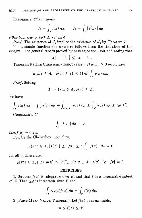
§43] DEFINITION AND PROPERTIES OF THE LEBESGUE INTEGRAL 55
THEOREM 8. The integrals
= IAj2
= L If(x) I
either both exist or both do not exist.Proof. The existence of J2 implies the existence of J1 by Theorem 7.For a simple function the converse follows from the definition of the
integral. The general case is proved by passing to the limit and noting that
hal - Ibtl � Ia - bt.THEoREM 9 (THE CHEBYSHEV INEQUALITY). If cc(x) � 0 on A, then
E A, � c} � (1/c) L
Proof. Setting
A' = Ix:x E � cj,
we have
IA = IA' + � �COROLLARY. If
fAtf(x)f = 0,
thenf(x) = 0 a.e.
For, by the Chebyshev inequality,
E A,If(x)l � 1/ni 0
for all n. Therefore,
b4x:x E A,f(x) O} � E A, f(x) I � 1/n) = 0.
EXERCISES
1. Suppose f(x) is integrable over E, and that F is a measurable subsetof E. Then XFf is integrable over E and
L XF(x)f(x) IFf(x)
2 (FIRST MEAN VALUE THEOREM). Let f(x) be measurable,
m<f(x) �M
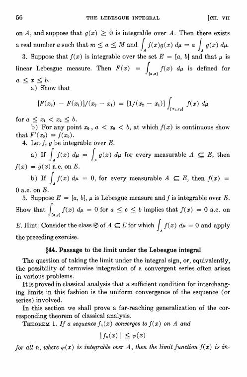
56 THE LEBESGUE INTEGRAL [CH. VII
on A, and suppose that g(x) � 0 is integrable over A. Then there exists
a real number a such that m < a � M and f f(x)g(x) d/2 = aL
g(x)
3. Suppose that f(x) is integrable over the set E = [a, b] and that is
linear Lebesgue measure. Then F(x) = f f(x) is defined for[ax]
a < x < b.
a) Show that
{F(x2) — F(x1)]/(x2 — = [1/(x2 — xi)] f f(x)[x1 ,X2]
for a � x1 < x2 � b.
b) For any point x0, a < xo < b, at which f(x) is continuous showthat F'(xo) = f(xo).
4. Let f, g be integrable over E.
a) If f f(x) = f g(x) for every measurable A E, then
f(x) = g(x) a.e. on E.
b) If f f(x) dji = 0, for every measurable A E, then f(x) =
0 a.e. on E.
5. Suppose E = [a, b], is Lebesgue measure and f is integrable over E.
Show that f f(x) = 0 for a � c b implies that f(x) = 0 a.e. on[ac]
E. Hint: Consider the class of A ç E for which f f(x) dji = 0 and apply
the preceding exercise.
§44. Passage to the limit under the Lebesgue integral
The question of taking the limit under the integral sign, or, equivalently,the possibility of termwise integration of a convergent series often arisesin various problems.
It is proved in classical analysis that a sufficient condition for interchang-ing limits in this fashion is the uniform convergence of the sequence (orseries) involved.
In this section we shall prove a far-reaching generalization of the cor-responding theorem of classical analysis.
THEOREM 1. If a sequence converges to f(x) on A and
I
� cc(x)
for all n, where çc(x) is integrable over A., then the limit function f(x) is in-

§44] PASSAGE TO THE LIMIT UNDER THE INTEGRAL 57
tegrable over A and
fAfnx
Proof. It easily follows from the conditions of the theorem that
If(x) I
LetAk= {x:k— 1 � cc(x) Uk�m+l Ak � m}.
By Theorem 6 of §43,
(*)IA
=fAk
and the series (*) converges absolutely.Hence
Lmçc(x) d/2
'[Ak
dji.
The convergence of the series (*) implies that there exists an m such that
IBm
The inequality cc(x) <m holds on A \ Bm By Egorov's theorem, A \ Bm
can be written as A \ Bm = C u D, where /2(D) < €/5m and the sequenceconverges uniformly to f on C.
Choose an N such that
f(x)I
<€/5/2(C)
for all n > N and x E C. Then
f — f(x)} = IBm -+ — + f[fn(x)
COROLLARY. If I � M and then
Lfnx LfxREMARK. Inasmuch as the values assumed by a function on a set of
measure zero do not affect the value of the integral, it is sufficient to assumein Theorem 1 that converges to f(x) a.e.

58 THE LEBESGUE INTEGRAL [OH. VII
THEOREM 2. Suppose that
fi(x) �f2(x) � �on a set A, where the functions are integrable and their integrals arebounded from above:
IA� K.
(1) f(x)
exists a.e. on A, f(x) is integrable on A and
LfnxClearly, the theorem also holds for a monotone descending sequence of
integrable functions whose integrals are bounded from below.On the set on which the limit (1) does not exist, f(x) can be defined
arbitrarily; for instance, we may set f(x) = 0 on this set.Proof. We assume that f(x) � 0, since the general case is easily reduced
to this case by writing
= — fi(x).We consider the set
= {x:x E
It is easy to see that = flr where
Ix:x E > r}.
By the Chebyshev inequality (Theorem 9, §43),
� K/r.
Since •, it follows that
K/r.
Further, since
cfor every r, K/r. Since r is arbitrary,
= 0.
This also proves that the monotone sequence f(x)a.e. on A.
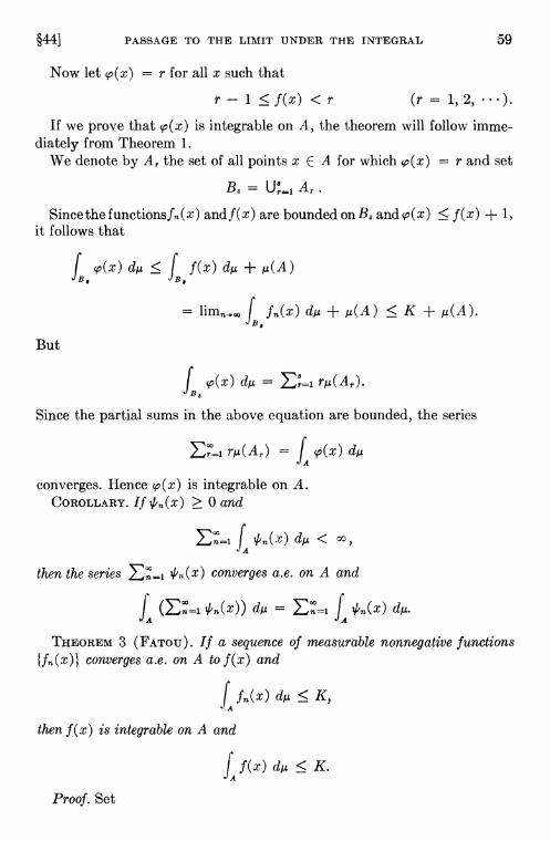
§44] PASSAGE TO THE LIMIT UNDER THE INTEGRAL 59
Now let co(x) = r for all x such that
r — 1 � f(x) < r (r = 1, 2, ).
If we prove that co(x) is integrable on A, the theorem will follow imme-diately from Theorem 1.
We denote by Ar the set of all points x E A for which cc(x) = r and set
B8 = Ar.
Since the functionsfn(x) andf(x) are bounded on B8 and co(x) � f(x) + 1,it follows that
+
= + � K +
But
lBs=
Since the partial sums in the above equation are bounded, the series
= IA
converges. Hence co(x) is integrable on A.COROLLARY. If
L <
then the series converges a.e. on A and
IA=
THEOREM 3 If a sequence of measurable nonnegative functions
converges a.e. on A to f(x) and
L � K,
then f(x) is integrable on A and
IA� K.
Proof. Set
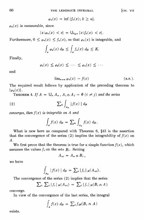
60 THE LEBESGUE INTEGRAL [OH. VII
inf {fk(x); k �is measurable, since
< c} = {x:fk(x) < c}.
Furthermore, 0 � ccn(x) � so that is integrable, and
IA � IA � K.
Finally,
coi(x) � � ... <
and
ccn(x) = f(x) (a.e.).
The required result follows by application of the preceding theorem totccn(x) }.
THEOREM 4. If A = A A 0 (i j) and the series
(2) If(x) I
converges, then f(x) is integrable on A and
IA= f(x)
What is new here as compared with Theorem 6, §43 is the assertionthat the convergence of the series (2) implies the integrability of f(x) onA.
We first prove that the theorem is true for a simple function f(x), whichassumes the values on the sets Setting
=
we have
fAn=
The convergence of the series (2) implies that the series
=converge.
In view of the convergence of the last series, the integral
Lfx = n A)
exists.

§441 PASSAGE TO THE LIMIT UNDER THE INTEGRAL 61
In the general case, we approximate f(x) by a simple function J(x) sothat
(3) f(x) —J(x) <€.
Then
7(x) I 1(x) I +
Since the series
=
converges, the convergence of (2) implies the convergence of
IJ(x) I
that is, in view of what has just been proved, the integrability of the simplefunction j'(x) on A. But then, by (3), 1(x) is also integrable on A.
EXERCISES
1. Let X = [0, fl, let be linear Lebesgue measure and suppose thatf(x) � 0 is measurable.
a) Suppose > > > > ..., —-f 0 and f(x) integrable overfl. Then f is integrable over [0, 1] if, and only if, f(x) d/2
exists, and in that case
f 1(x) = f f(x)10,1]
(This justifies the remark made at the end of §45.)2. For f(x) measurable on the measurable set B define
= 1(x) < (k + x E E}, n = 1, 2,
a) If f is integrable on B, then each is absolutely convergent,exists and
=
b) Conversely, if converges absolutely for some n, then con-verges absolutely for all n, f(x) is integrable over B and the above equalityholds.
c) Let n = 0 in a). It follows that
< oo.

62 THE LEBESGUE INTEGRAL [cH. VII
Show consequently that f integrable over B implies that
rn/i{x: f(x) � m, X E E} = 0.
Hint: Reduce the problem to the case f(x) � 0.3. Let X be measurable, and let (a, b) be an interval of real numbers.
Suppose f(x, t) is real-valued for x E X, t E (a, b) and that it satisfies thefollowing:
(i) For t E (a, b), f(x, t) is integrable over X.(ii) 3f(x, t)/at exists for all t E (a, b) and there exists a function 8(x)
integrable over X for which
3f(x, t)/at � 8(x) [x E X, t E (a, b)].
Show that
d/dtff(x,t) =
Hint: For t0 E (a, b) the limit defining the derivative can be obtained byusing a sequence { in (a, b), to. Apply Theorem 1.
§45. Comparison of the Lebesgue and Riemann integralsWe shall discuss the relation of the Lebesgue integral to the usual Rie-
mann integral. In doing so, we restrict ourselves to the simplest case, linearLebesgue measure on the real line.
THEOREM. If the Riemann integral
J = (R)f
f(x) dx
exists, then f(x) is Lebesgue integrable on [a, b], and
f[a,b]
Proof. Consider the partition of [a, b] into subintervals by the points
xk a+ — a)
and the Darboux sums
= (b —
= (b —
where is the least upper bound of f(x) on the interval
Xk_1 � x � xk,

§45] COMPARISON OF LEBESGUE AND RIEMANN INTEGRALS 63
and is the greatest lower bound of f(x) on the same interval. By defi-nition, the Riemann integral is
J = =
We set
= (Xk_1 X
= (Xk_1 X <Xk).
The functions and can be extended to the point x = b arbitrarily. Itis easily verified that
f =(a,b]
f(a,b]
Since is a nonincreasing sequence and is a nondecreasing sequence,
�f(x),<f(x)
a.e. By Theorem 2 of §44,
f J(x) dM = = J = = f f(x)(a,b] [a,b]
Therefore,
f J(x)= f {J(x)
[a,b] [a,b]
consequently,
J(x) —1(x) =0a.e., i.e.,
J(x) = f(x) =
f[a,b] [a,b]
This proves the theorem.TRANS. NOTE. The following well known characterization of Riemann
integrable functions now follows immediately from the preceding theoremand the observation that f(x) is continuous at x if, and only if, J(x) =

64 THE LEBESGUE INTEGRAL [CH. vii
Let f(x) be bounded on [a, b}. Then f(x) is Riemann integrable if, and onlyif, it is continuous a.e.
It is easy to construct an example of a bounded function which is Lebesgueintegrable but not Riemann integrable (for instance, the Dirichiet functionmentioned above).
An arbitrary functionf(x) for which the Riemann integral
If(x) dx
approaches a finite limit J as 0 is Lebesgue integrable on [0, 1], and
f = f f(x) dx.(0,1]
(See Ex. 4, §44.)In this connection it is interesting to note that the improper integrals
jf(x) dx = 1(x) dx,
where
If(x)
I
dx =
cannot be taken in the sense of Lebesgue: Lebesgue integration is absoluteintegration in the sense of Theorem 8, §43.
EXERCISES
1. Let f(x), g(x) be Rieinann integrable functions on [a, b}. Thenf(x)g(x) is Riemann integrable on [a, b]. This fact can be proved withoutthe characterization of Riemann integrable functions given in the text, buta direct proof is difficult.
2. A nondecreasing (nonincreasing) real-valued function defined on aninterval [a, b} is Riemann integrable on this interval.
3. Show that the function
f(x) = d/dx(x2 sin 1/x2) = 2x sin 1/x2 — (2/x) cos 1/x2
is not Lebesgue integrable over [0, 11, although f(x) is continuous on [€, 1]
for every 0 and f f(x) dx exists; that is, f(x) is improperly
Riemann integrable, the integral being only conditionally convergent.Hint: I f(x)
I� (2/x) cos 1/x2 I — 2x � — 2x on each of the inter-
vals {(2n + � x � {(2n —

§461 PRODIJCTS OF SETS AND MEASURES 65
§46. Products of sets and measuresTheorems on the reduction of double (or multiple) integrals to repeated
integrals play an important part in analysis. The fundamental result in thetheory of multiple Lebesgue integrals is Fubini's theorem, which we shallprove in §48. We first introduce some auxiliary concepts and results which,however, have an interest independent of Fubini's theorem.
The set Z of ordered pairs (x, y), where x E X, y E Y, is called theproduct of the sets X and V and is denoted by X X Y. In the same way,the set Z of finite ordered sequences (xi , ••' , where Xk E Xk , is calledthe product of the sets X1, , and is denoted by
Z = X1 x X2 x x =
In particular, if
x1=x2= ... =xn=x,the set Z is the nth power of the set X:
z =
For instance, the n-dimensional coordinate space is the nth power ofthe real line D'. The unit cube Jfl, that is, the set of points of with co-ordinates satisfying the conditions
is the nth power of the closed unit interval J' = [0, 1].
If , are collections of subsets of the sets Xi, •' , then
is the collection of subsets of the set X = X k Xk representable in the form
A = A1 X x (Ak E
If = = = = then is the nth power of
For instance, the set of all parallelopipeds in is the nth power of the setof closed intervals in D1.
THEOREM 1. If , are semi-rings, then = X k is a semi-ring.Proof. In view of the definition of a semi-ring we must prove that
if A, B E then A n B E and if, moreover, B ç A, then A =
We shall carry out the proof for n = 2.

66 THE LEBESGUE INTEGRAL [cH. VII
I) Suppose that A, B E X Then
B = B1 X B2, B1 E B2 E
Hence
A n B = (A1 n B1) x (A2 n B2),
and since
A nB E X
II) Now, on the same assumptions as in I), suppose that B A. Then
B1çA1, B2c_A2,
and because and are semi-rings, it follows that(1) (k)A1=B1uB u'uB1
(1) (1),
A = A1 X A2 = (B1 X B2) U (Bi X u ••• u (B1 x
u x B2) u x u • • • u (B1u) X
u x B2) u X B2'") U • • U xIn the last relation the first term is B1 X B2 = B and all the other terms
are elements of X (all pairwise disjoint). This proves the theorem.However, if the are rings or Borel rings, it does not follow that X
is a ring or a Borel ring.Suppose that the measures
, (Ak E
are defined on the semi-rings ,
We define the measure
on
by the following condition: If A = A1 X X , then
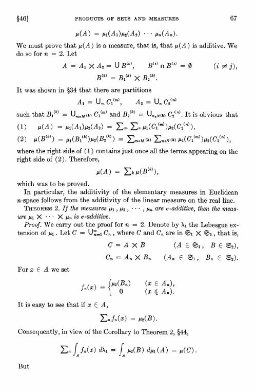
§46] PRODUCTS OF SETS AND MEASURES 67
= •••
We must prove that .4(A) is a measure, that is, that /.4(A) is additive. Wedo so for n = 2. Let
A = A1 X A2 = U B(t) n = 0 (i= X
It was shown in §34 that there are partitionsII cy(m) A — II çy(n)
— '-'1 , — "2
such that = UmEM(k) C1(m) and = UflEN(k) C2. It is obvious that
(1) /.L(A) = = En(2) = = /.Ll(Cl(m)
where the right side of (1) contains just once all the terms appearing on theright side of (2). Therefore,
IA\ / (/c)\— ),
which was to be proved.In particular, the additivity of the elementary measures in Euclidean
n-space follows from the additivity of the linear measure on the real line.THEOREM 2. If the measures , , are r-additive, then the meas-
ure X X is r-additive.Proof. We carry out the proof for n = 2. Denote by Xi the Lebesgue ex-
tension of Let C = where C and are in X that is,
C=AXBCnAnXBn E E
For x E A we set
(x E An),fflX0
It is easy to see that if x E A,
= p2(B).
Consequently, in view of the Corollary to Theorem 2, §44,
dX1= IA
=
But
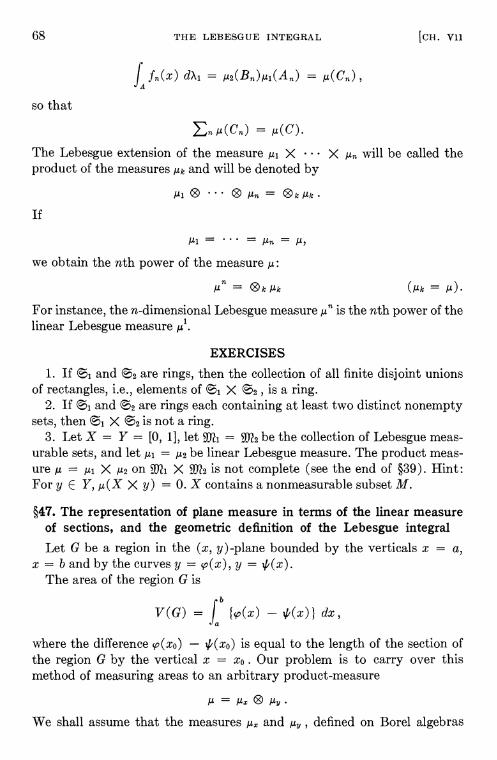
68 THE LEBESGUE INTEGRAL [CH. vii
L dX1 = =
so that
=
The Lebesgue extension of the measure X X will be called theproduct of the measures and will be denoted by
/21®" ®12n=®k/2k.
we obtain the nth power of the measure
/2 = ®k/.4k (/hk =
For instance, the n-dimensional Lebesgue measure is the nth power of thelinear Lebesgue measure
EXERCISES
1. If and are rings, then the collection of all finite disjoint unionsof rectangles, i.e., elements of X is a ring.
2. If and are rings each containing at least two distinct nonemptysets, then x is not a ring.
3. Let X = V = [0, 1], let = be the collection of Lebesgue meas-urable sets, and let = /22 linear Lebesgue measure. The product meas-ure = X /22 on X is not complete (see the end of §39). Hint:For y E Y, p.(X X y) = 0. X contains a nonmeasurable subset M.
§47. The representation of plane measure in terms of the linear measureof sections, and the geometric definition of the Lebesgue integralLet G be a region in the (x, y)-plane bounded by the verticals x = a,
x = band by the curves y = y =The area of the region G is
V(G) = L — dx,
where the difference — is equal to the length of the section ofthe region G by the vertical x = x0. Our problem is to carry over thismethod of measuring areas to an arbitrary product-measure
/2 = ® /2g.
We shall assume that the measures and defined on Borel algebras
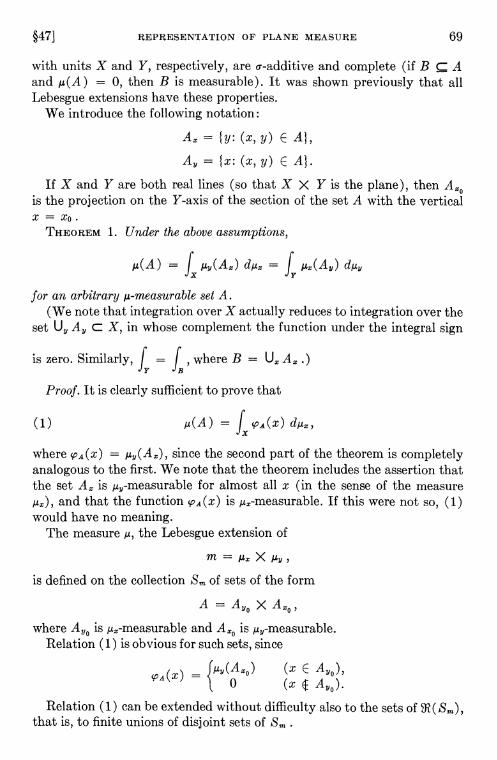
§47] REPRESENTATION OF PLANE MEASURE 69
with units X and Y, respectively, are r-additive and complete (if B ç Aand /.L(A) = 0, then B is measurable). It was shown previously that allLebesgue extensions have these properties.
We introduce the following notation:
ty: (x, y) E A},
= tx: (x, y) E A}.
If X and V are both real lines (so that X X Y is the plane), thenis the projection on the V-axis of the section of the set A with the verticalx = xo.
THEOREM 1. Under the above assumptions,
= = ffor an arbitrary 1.4-measurable set A.
(We note that integration over X actually reduces to integration over theset C X, in whose complement the function under the integral sign
is zero. Similarly, f= fB' where B = As.)
Proof. It is clearly sufficient to prove that
(1) =
where = since the second part of the theorem is completelyanalogous to the first. We note that the theorem includes the assertion thatthe set is for almost all x (in the sense of the measure
and that the function is If this were not 50, (1)would have no meaning.
The measure /2, the Lebesgue extension of
m = 1.4z X
is defined on the collection Sm of sets of the form
A = xwhere is and is
Relation (1) is obvious for such sets, since
— (x E—0 (x
Relation (1) can be extended without difficulty also to the sets ofthat is, to finite unions of disjoint sets of Sm.

70 THE LEBESGIJE INTEGRAL [CH. VII
The proof of (1) in the general case is based on the following lemma,which has independent interest for the theory of Lebesgue extensions.
LEMMA. If A is a 1.4-measurable set, there exists a set B such that
B = B1 B2 D••,Bfl = Uk Bflk,
where the sets are elements of ( Sm), A ç B and
(2) p.(A) = /.4(B).
Proof. The proof is based on the fact that, according to the definition ofmeasurability, for arbitrary n the set A can he included in a union
Cn = Ur
of sets of Sm such that </.4(A) + 1/n.Setting Bfl = Elk , it is easily seen that the sets will have the form
Bfl = , where the sets are elements of Sm. Finally, putting
Bnk — s=1t-1fl8,
we obtain the sets required by the lemma.Relation (1) is easily extended with the aid of the sets Bflk E (Sm) to
the sets B by means of Theorem 2, §44, since
= � �= � �
If = 0, then = 0, and
= = 0
a.e. Since is measurable for almost all x and
= 0,
f = 0 =
Consequently, relation (1) holds for sets A such that = 0. If A isarbitrary, we write it as A = B \ C, where, in view of (2),
= 0.
Since (1) holds for B and C, it is easy to see that it also holds for A.This completes the proof of Theorem 1.We now consider the special case when Y is the real line, is linear
Lebesgue measure and A is the set of points (x, y) such that

§47] REPRESENTATION OF PLANE MEASURE 71
3fxEM,
where M is a set and f(x) is an integrable nonnegative func-tion. Then
'A \ — Jf(x) (x E M),0 (xEEM),
= fM
We have proved the followingTHEOREM 2. The Lebesgue integral of a nonnegative integrable function
f(x) is equal to the measure = of the set A defined by (3).If X is also the real line, the set M a closed interval and the function
f(x) Riemann integrable, this theorem reduces to the usual expression forthe integral as the area under the graph of the function.
EXERCISES
1. The assumption that < and Y) < or more generallythat X and Y are countable unions of sets of finite measure cannot bedropped from Theorem 1. Let X = Y = [0, 1], let be the class of Lebes-gue measurable sets of X, Lebesgue measure, the class of all subsetsof Y, the number of points in A, A Y. If E = { (x, y) x =
show that f = 1, but f = 0.
2. Under the hypotheses of Theorem 2, the graph of a nonnegativemeasurable function, i.e., { (x, f(x)) :x E has /2-measure zero.
3. Let X = Y = [0, 1], let = be linear Lebesgue measure and set= ® Suppose that A X is nonmeasurable and that B ç V is
such that = 0.
a) XAXB(X, y) is /1-measurable.b) XAXB(X, y) is for almost all (but not all) y E Y.
4. If A and B are measurable subsets of X X Y, i.e., = ®measurable, and = for almost every x E X, then
/1(A) =
5. Suppose v = f(u) is a strictly increasing continuous function definedon [0, cia) with f(0) = 0 and = Then u = f1(v) = g(v)also has all these properties. Suppose that 0 u0 < 0 vo <U = [0, uo], V = [0, Vo], and = is linear Lebesgue measure. Let
F(uo) = f f(u) G(vo) = f g(v)(O,u0] (O,v0]
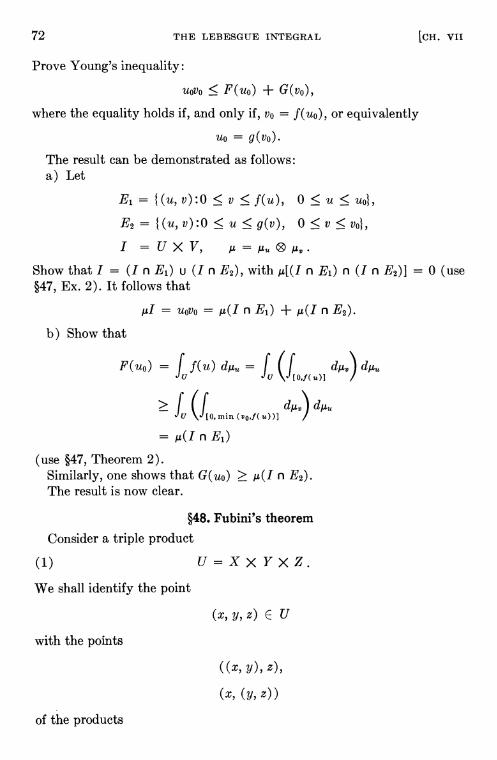
72 THE LEBESGUE INTEGRAL [CH. vii
Prove Young's inequality:
uovo � F(uo) + G(vo),
where the equality holds if, and only if, = f(uo), or equivalently
= g(vo).
The result can be demonstrated as follows:a) Let
B1 = {(u, v):O v � f(u), 0 � u �B2 = {(u, v):O u g(v), 0 � vI =UXV, /.L/2u®/.Lv.
Show that I = (I n B1) u (I n E2), with n Bi) n (I n E2)] = 0 (use§47, Ex. 2). It follows that
= u0v0 = n B1) + /2(1 n E2).
b) Show that
F(uo) = f f(u) = f (fU U [0,1(u)]
� f (fU [0mm (vo,f(u))1
= /2(1 n E1)
(use §47, Theorem 2).Similarly, one shows that G(uo) � n E2).The result is now clear.
§48. Fubini's theorem
Consider a triple product
(1) u=xxyxz.We shall identify the point
(x, y, z) E U
with the points
((x, y), z),
(x, (y, z))
of the products

§48] FTJBINI'S THEOREM 73
(2) (XxY)xZ,(3) XX(YXZ).
We therefore agree to regard the products (1), (2) and (3) as identical.If measures are defined on X, Y, Z, then the measure.
1hz ® /2y ® Mz
may be defined as
= (j.&x ® ®
or as
12u = /1z ® ®
We omit a rigorous proof of the equivalence of these definitions, althoughit is not difficult.
We shall apply these general ideas to prove the fundamental theorem ofthe theory of multiple integrals.
FuBINI's THEOREM. Suppose that a-additive and complete measures andare defined on Borel algebras with units X and Y, respectively; further, sup-
pose that
= 1hz ® 1hy,
and that the function f(x, y) is /2-integrable on
A = X
Then (see the parenthetical remark on p. 69)
= f1(L f(x,y)(4)
= L (Lf(x, y)
Proof. The theorem includes among its assertions the existence of theintegrals in parentheses for almost all values of the variables with respectto which the integrals are taken.
We shall prove the theorem first for the case f(x, y) � 0. To this endconsider the triple product
U=XXYXD1,where the third term is the real line, and the product measure
where is linear Lebesgue measure.

74 THE LEBESGUE INTEGRAL [CII. VII
We define a subset W of U as follows:
(x, y, z) E W
0 z _<f(x,y).
In view of Theorem 2, §47,
(5) x(W)IA
On the other hand, by Theorem 1, §47,
(6) x(W) = fwhere ® and is the set of pairs (y, z) for which (x, y, z) E W.By Theorem 2, §47,
(7) = L y)
Comparing (5), (6), and (7), we obtain
IA = fX(fAf(x,Y)
This completes the proof of the theorem if f(x, y) � 0. The general caseis reduced to the case f(x, y) � 0 by means of the relations
f(x,y) —f(x,y),
f(x, y) f(x, y)], f(x, y) = f(x, I — f(x, y)].
REMARK. It can be shown that if f(x, y) is /h-measurable, then
exists if
L f(x, y) I
exists.EXAMPLES where (4) does not hold.1. Let
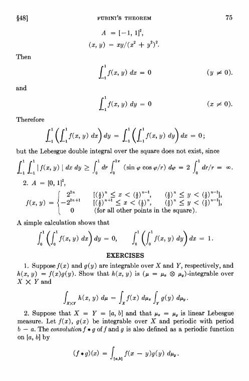
§481 FUBINI'S THEOREM 75
A = [—1, 1]2,
(x, y) = xy/(x2 + y2)2.
Then
ff(x, y) dx = 0 (y 0).
and
ff(x, y) dy = 0 (x 0).
Therefore
(ff(x, y) dx) dy = f (ff(x, y) dy) dx = 0;
but the Lebesgue double integral over the square does not exist, sinceg'l
J J I f(x, y) I dx dy � / dr J (sin cos W/r) = 2 Jdr/r =
—1—1 •0 0 0
2. A = [0, 112,
I < x < <<
f(x, y) = _22n+1 < x <<
<
0 (for all other points in the square).
A simple calculation shows that
f' y) dx) dy = f' y) dy) dx = 1.
EXERCISES
1. Suppose f(x) and g(y) are integrable over X and Y, respectively, andh(x, y) = f(x)g(y). Show that h(x, y) is = ® overX X Y and
h(x, y) = f 1(x) f g(y)
2. Suppose that X = Y = [a, b] and that = is linear Lebesguemeasure. Let f(x), g(x) be integrable over X and periodic with periodb — a. The convolution f * g of f and g is also defined as a periodic functionon [a, b] by
(f*g)(x) = f f(x — y)g(y)[a,bl

THE LEBESGUE INTEGRAL [CH. VII
Show that (f * g)(x) is integrable over X and
L f(f*g)(x)f ff(y)f
I
g demonstrates the existence of (f * g) (x) for almostall x E X. Hint: Use Fubini's theorem.
3. Suppose that f(x) is integrable over [0, b] with respect to Lebesguemeasure. Suppose that a > 0. The ath fractional integral of f is defined by
Ia(f)(X) = [F(a)]' f (x —[Ox]
for x E [0, b], where F(a) is the Gamma function. Show that Ia(f)(X)defined a.e. on [0, b} and is integrable over [0, a] for a E [0, b]. Hint: Dodirectly as in Ex. 2, or use a suitable convolution of f(x) with anotherfunction.
4. Suppose that a > 0, /3 > 0, f(x) is integrable on [0, b] with respectto Lebesgue measure. By Ex. 3, is defined a.e. on [0, b]. Showthat
Hint: Use the result: for p > 0, q > 0,
f— = p(p)p(q)/J1(p +
[0,1]
5. (INTEGRATIoN BY PARTS.) Let X = V [0, b] and let /.L = ® /h11,where is linear Lebesgue measure.
Suppose that f(x), g(x) are integrable over X. If
F(x) =f G(x) = [[Ox] [Ox]
for x E [0, 1], then
f F(x)g(x) = F(b)G(b) L f(x)G(x)
The result may be demonstrated as follows:a) Let E = { (x, y): (x, y) E X X Y, y � Show that E is
urable. Hence XE is /h-measurable and H(x, y) = XE(X, y)g(x)f(y) is also/2-measurable.
b) Show that H(x, y) is integrable over X X Y with respect to(Apply Ex. 1.)
c) Apply Fubini's theorem to obtain

§49] THE INTEGRAL AS A SET FUNCTION 77
f F(x)g(x) = f H(x, y)= f f(y)
(fg(x)
I XXY Y [Ybl
This will yield the stated result.
§49. The integral as a set function
We shall consider the integral F(A)= f f(x) d/2 as a set function on
the assumption that is a Borel algebra with unit X and that I f(x)
exists.Then, as we have already proved:1. F(A) is defined on the Borel algebra ASH.2. F(A) is real-valued.3. F(A) is additive, that is, if
A = E ASH)'
then
F(A) =4. F(A) is absolutely continuous, that is, /1(A) = 0 implies that
F(A) 0.
We state the following important theorem without proof:RADON'S THEOREM. If a set function F(A) has properties 1, 2, 3 and 4, it
is representable in the form
F(A) = fAfxWe shall show that the function f = is uniquely defined a.e. In
fact, if
F(A)= IA fi(x) =
for all A E then
<nf(fi = 0
for arbitrary n, where
= {x:fi(x) — f2(x) > 1/ni.
Similarly,

78 THE LEBESGUE INTEGRAL [CH. VII
= 0
for
= {x:f2(x) — fi(x) > 1/ni.Since
{x:fi(x) UnAnUUmBm,
it. follows that
0.
This proves our assertion.
EXERCISES
1. With the notation of this section, suppose that f(x) � 0 and let
v(A) f f(x) Then the conditions listed before Radon's theorem
can be paraphrased by saying that v(A) is a completely additive, absolutelycontinuous measure on the Borel algebra . Show that if g(x) is integrableover X with respect to ii, then
fAg(x) dv
= f f(x)g(x) (A E Sn).
2. If v(A) is a completely additive measure on the Borel algebrathen v may have the following property: For 0 there exists a > 0such that A E and /2(A) < imply v(A) < It is easy to see that ifv has this property, then ii is absolutely continuous with respect to /1, i.e.,
0 implies v(A) = 0. Show, conversely, that if v is absolutely con-tinuous with respect to then v has the above property.

Chapter VIII
SQUARE INTEGRABLE FUNCTIONS
One of the most important linear normed spaces in Functional Analysisis filbert space, named after the German mathematician David filbert,who introduced this space in his research on the theory of integral equa-tions. It is the natural infinite-dimensional analogue of Euclidean n-space.We became acquainted with one of the important realizations of filbertspace in Chapter Ill—the space 12, whose elements are the sequences
x (x1, •.. )
satisfying the condition
n=lxn <
We can now use the Lebesgue integral to introduce a second, in certainrespects more convenient, realization of filbert space—the space of squareintegrable functions. In this chapter we consider the definition and funda-mental properties of the space of square integrable functions and showthat it is isometric (if certain assumptions are made about the measureused in the integral) to the space 12.
We shall give an axiomatic definition of filbert space in Chapter IX.
§50. The space L2
In the sequel we consider functions f(x) defined on a set R, on which ameasure /2(E) is prescribed, satisfying the condition /h(R) < oo• Thefunctions f(x) are assumed to be measurable and defined a.e. on R. Weshall not distinguish between functions equivalent on R. For brevity,
instead of we write simply f.
DEFINITIoN 1. We say that f(x) is a square integrable (or summable)function on R if the integral
f f2(x)
exists (is finite). The collection of all square integrable functions is denotedby L2.
The fundamental properties of such functions follow.THEOREM 1. The product of two square integrable functions is an integrable
function.
79

80 SQUARE INTEGRABLE FUNCTIONS [CH. VIII
The proof follows immediately from the inequality12 2f(x)g(x) I (x) + g (x)]
and the properties of the Lebesgue integral.COROLLARY 1. A square integrable function f(x) is integrable.For, it is sufficient to set g(x) 1 in Theorem 1.THEOREM 2. The sum of two functions of L2 is an element of L2.Proof. Indeed,
[f(x) + g(x)]2 + 2 f(x)g(x) + g2(x)and Theorem 1 implies that the three functions on the right are summable.
THEOREM 3. If f(x) E L2 and a is an arbitrary number, then a f(x) E L2.Proof. If f E L2, then
f = 2ff2()d <
Theorems 2 and 3 show that a linear combination of functions of L2is an element of L2; it is also obvious that the addition of functions andmultiplication of functions by numbers satisfy the eight conditions of thedefinition of a linear space (Chapter III, §21). Hence L2 is a linear space.
We now define an inner (or a scalar) product in L2 by setting
(1) (f,g)
An inner product is a real-valued function of pairs of vectors of a linearspace satisfying the following conditions:
1) (f,g) = (g,f).2) (fi+f2,g) = (fi,g) + (f2,g).3) (Xf,g) = X(f,g).4) (f,f)The fundamental properties of the integral immediately imply that
Conditions 1 )—3) are satisfied by (1). Inasmuch as we have agreed not todistinguish between equivalent functions (so that, in particular, the nullelement in L2 is the collection of all functions on R equivalent to f = 0),Condition 4) is also satisfied (see the Corollary to Theorem 9, §43). Wetherefore arrive at the following
DEFINITIoN 2. The space L2 is the Euclidean space (a linear space withan inner product) whose elements are the classes of equivalent squareintegrable functions; addition of the elements of L2 and multiplication byscalars are defined in the way usual for functions and the inner product is

§50] THE SPACE L2 81
defined by
(1) (f,g) =
The Schwarz inequality, which in this case has the form
(2) (1 f 12(x) g2(x)
is satisfied in L2, as it is in every Euclidean space (see Ex. 3, §56). Thesame is true for the triangle inequality
(3) [1(x) + g(x)]2 � 12(x)+ {f
In particular, the Schwarz inequality yields the following useful in-equality:
(4) (f 1(x) 5; f 12(x)
To introduce a norm into L2 we set
(5) = = (IEL2).
EXERCISE. Using the properties 1 )—4) of the inner product, prove thatthe norm defined by (5) satisfies Conditions 1—3 of the definition of anorm in §21.
The following theorem plays an important part in many problems ofanalysis:
THEOREM 4. The space L2 is complete.
Proof. a) Let be a fundamental sequence in L2, i.e.,
Then there is a subsequence of indices {nkl such that
II fnk — II 5;(1)k
Hence, in view of inequality (4), it follows that
f — lflk+1(x) I 5; {f— lnk+1(x)}2
<
This inequality and the Corollary to Theorem 2, §44 imply that the series
I I +

82 SQUARE INTEGRABLE FUNCTIONS [CH. VIII
converges a.e. on R. Then the series
+ Lfn2(X) — +
also converges a.e. on R to a function
(6) f(x) =Hence, we have proved that if is a fundamental sequence of func-tions in L2, it contains an a.e. convergent subsequence.
b) We shall now show that the function f(x) defined by (6) is anment of L2 and that
(7) —f(x) (n—*
For sufficiently large k and 1,
f —
In view of Theorem 3, §44, we may take the limit under the integralsign in this inequality as 1 —* We obtain
f �It follows that f E L2 and fflk f. But the convergence of a subsequenceof a fundamental sequence to a limit implies that the sequence itself con-verges to the same limit. [Convergence here means the fulfillment of (7);in this connection see §51.] This proves the theorem.
EXERCISES
1. If we define the distance d(f1 , 12) in L2(R, as
d(f1,f2) = — f211 = {f[fi(x) —
then d satisfies the axioms for a metric space (see vol. 1, §8). Further-more, d is translation invariant, i.e.,
d(f1 + f, f2 + f) = d(f1 , f2)
for f E L2. This result, of course, holds in any normed linear space(see vol. 1, §21).
2. Let R [0, 1] and let be linear Lebesgue measure. Show that{f: f � 1} is closed and bounded, but not compact.
3. With the notation of Ex. 2, show that the set of continuous functionson [0, 1] is a linear manifold in L2, but is not a subspace, i.e., is not closed.(For the terminology, see §57.)

§50] THE SPACE L2 83
4. A measurable function f(x) is said to be essentially bounded (on R)if there exists an a > 0 such that I f(x) < a a.e. on R. The number a iscalled an essential upper bound of f on R. For an essentially bounded func-tion f, let m = inf { a : a an essential upper bound of The number m iscalled the essential supremum of f: m = ess. sup f.
a) Show that ess. sup f is the smallest essential upper bound of f on R.b) Let L00(R, be the collection of essentially bounded functions on
R. If we put f IJ = ess. sup f, show that Lc,3 becomes a normed linearspace.
5. Let LP(R, /2), p � 1, be the set of measurable functions f defined onR for which I f(x) is integrable over R.
a) If a, b are real numbers, show that
(The condition p > 1 is essential here.)b) Show then that is a linear space, i.e., f, g E implies that
f + g E and that f E and a real imply af E Define f =lip
[JR f(x) . We shall shortly see that is a normed space with
f as norm.6. a) Suppose p > 1. Define q by the equation i/p + 1/q = 1. p and q
are called conjugate exponents. Let v = f(u) = Then u = g(v) =Verify that the hypotheses of Young's inequality Ex. 5) are satisfiedand that F(u) = un/p, G(v) = and that therefore
uv � u9p +with equality if, and only if, =
b) (HoLDER INEQUALITY.) Suppose f E g E Lq(R, withp, q conjugate exponents. Show that
f(x)g(x) E L1(R, = L
and
d/2 � JR f(x)g(x)
i/p 1/q
(JR Jf(x) (JRg(x)
=
This result may be obtained as follows: It is trivial ifJJ f 0 or
H g = 0. Otherwise, put

84 SQUARE INTEGRABLE FUNCTIONS {CH. VIII
u = If(x) / If v = g(x) I / IJ Ilq
in the result of a), and integrate over R (see vol. 1, p. 20).c) (MINK0wSKI'S INEQUALITY.) If f, g E ii), then
� Ifor, in terms of integrals,
(fRf(x) + g(x) P � (L I f(x) P
+ (f I g(x) dy).If 1 1 + g = 0, then the result is clear. If f + g 1T > 0, observe
that
If(x) + g(x) � I f(xfl f(x) + g(x)
Ig(x) In',
If(x) + g(x) E Lq.
Apply Holder's inequality to each term on the right to obtain1/q
fRI � (fRIf+ +
It is now clear that with norm f is a normed linear space forp > 1. Note also that if p = 2, then q = 2, and Holder's inequality re-duces to the Schwarz inequality.
§51. Mean convergence. Dense subsets of L2
The introduction of a norm in L2 determines a new notion of convergencefor square integrable functions:
(inL2)
f — f(x)]2 = 0.
This type of convergence of functions is called mean convergence, or,more precisely, mean square convergence.
Let us consider the relation of mean convergence to uniform convergenceand convergence a.e. (see Chapter VI).
THEOREM 1. If a sequence (x)1 of functions of L2 converges uniformlyto f(x), then f(x) E L2, and 'is mean convergent to f(x).
Proof. Suppose that 0. If n is sufficiently large,
f(x) <€,whence

§51] MEAN CONVERGENCE. DENSE SUBSETS OF L2 85
f — f(x)}2 <
The theorem follows at once from this inequality.Theorem 1 implies that if an arbitrary f E L2 can be approximated with
arbitrary accuracy by functions E M L2 in the sense of uniform con-vergence, then it can be approximated by such functions in the sense ofmean convergence.
Hence an arbitrary function f E L2 can be approximated with arbitraryaccuracy by simple functions belonging to L2.
We prove that an arbitrary simple function f E L2, and consequentlyan arbitrary function of L2, can be approximated to any desired degree ofaccuracy by simple functions whose set of distinct values is finite.
Suppose that f(x) assumes the values Yi, , on the setsE1, , Inasmuch as f2 is summable, the series
= ff2()
converges. Choose an N such that
< €,
and set
If(x) (x E � N),fN(X) -
Then
f [f(x) — fN(x)12 — L>N
that is, the function fN(X), which assumes a finite set of values, approxi-mates the function f with arbitrary accuracy.
Let R be a metric space with a measure possessing the following property(which is satisfied in all cases of practical interest): all the open and closedsets of R are measurable, and
(*) = cGIfor all M R, where the lower bound is taken over all open sets G con-taining M. Then we have
THEOREM 2. The set of all continuous functions on R is dense in L2.Proof. In view of the preceding discussion, it is sufficient to prove that
every simple function assuming a finite number of values is the limit, inthe sense of mean convergence, of continuous functions. Furthermore,

SQUARE INTEGRABLE FUNCTIONS {CH. VIII
since every simple function assuming a finite set of values is a linear com-bination of characteristic functions XM(X) of measurable sets, it is enoughto carry out the proof for such functions. Let M be a measurable set inthe metric space R. Then it follows at once from the Condition (*) thatfor every 0 there exists a closed set FM and an open set GM such that
FM ç M C GM, /.L(GM) — /2(FM) < €.
We now define
= p(x, R \ GM)/[p(x, R \ GM) + p(x, FM)].
This function isO on R \ GM and 1 on FM. It is continuous, since p(x, FM),p(x, R \ GM) are continuous and their sum does not vanish. The functionXM(X) — is bounded by 1 on GM \ FM and vanishes in the comple-ment of this set. Consequently,
f [XM(X) —
and the theorem follows.THEOREM 3. If a sequence converges to f(x) in the mean, it con-
lains a subsequence {fflk (x) which converges to f(x) a.e.Proof. If converges in the mean, it is a fundamental sequence in
L2. Therefore, repeating the reasoning in Part a) of the proof of Theorem4, §50, we obtain a subsequence {fflk(x)1 of which converges a.e.to a function Furthermore, Part b) of the same proof shows that{fnk(x)} converges to in the mean. Hence, = f(x) a.e.
* It is not hard to find examples to show that convergence in the meandoes not imply convergence a.e. In fact, the sequence of functionsdefined on p. 45 obviously converges in the mean to f 0, but (as wasshown) does not converge a.e. We shall now show that convergence a.e.(and even everywhere) does not imply mean convergence. Let
In {x E (0, 1/n)],=
0 for all remaining values of x.
It is clear that the sequence (x )} converges to 0 everywhere on [0, 1],but that
ff2() dx = n
The Chebyshev inequality Theorem 9) implies that if a sequenceis mean convergent, it converges in measure. Therefore, Theorem 3, whichwe have proved in this section independently of the Chebyshev inequality,
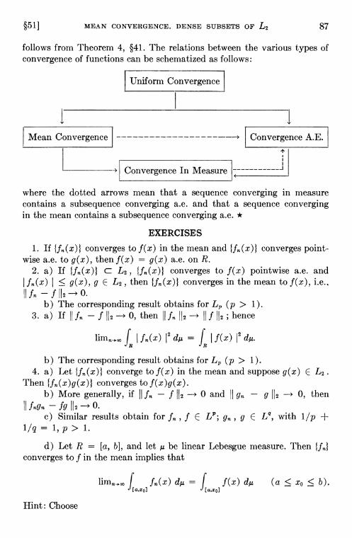
§51] MEAN CONVERGENCE. DENSE SUBSETS OF L2 87
follows from Theorem 4, §41. The relations between the various types ofconvergence of functions can be schematized as follows:
Uniform Convergence
I IMean Convergence - ——---f Convergence A.E.
Convergence In Measure
where the dotted arrows mean that a sequence converging in measurecontains a subsequence converging a.e. and that a sequence convergingin the mean contains a subsequence converging a.e. *
EXERCISES
1. If {fn(x)1 converges to f(x) in the mean and {fn(X)} converges point-wise a.e. to g(x), thenf(x) = g(x) a.e. on R.
2. a) If c: L2, converges to f(x) pointwise a.e. andI I � g(x), g E L2, then {fn(x)} converges in the mean to f(x), i.e.,
b) The corresponding result obtains for (p > 1).3. a) If — f 112 0, then
2 1' 2
J If(x)
b) The corresponding result obtains for (p > 1).4. a) Let converge to f(x) in the mean and suppose g(x) E L2.
Then converges to f(x)g(x).b) More generally, if f 1k 0 and — g 112 0, then
c) Similar results obtain for f E gn, g E J}, with i/p +1/q = 1, p> 1.
d) Let R = [a, b], and let be linear Lebesgue measure. Thenconverges to f in the mean implies that
f f f(x) (a � x0 � b).[ax0] [a,xo]
Hint: Choose

88 SQUARE INTEGRABLE FUNCTIONS ECH. VIII
Ii (a�x<xo),g(x) =
(x > xo).
Show that g E L2.
§52. L2 spaces with countable bases
The space L2 of square integrable functions depends, in general, on thechoice of the space R and the measure To designate it fully it should bewritten as L2(R, /2). The space L2(R, is finite-dimensional only in excep-tional cases. The spaces L2(R, which are most important for analysisare the spaces which have infinite dimension (this term will be explainedbelow).
To characterize these spaces, we need an additional concept from thetheory of measure.
We can introduce a metric in the collection of measurable subsets ofthe space R (whose measure we have assumed to be finite) by setting
p(A, B) = B).
If we identify sets A and B for which /2(A B) = 0 (that is, we considersets which are the same except for a set of measure zero to be indistin-guishable), then the set together with the metric p becomes a metricspace.
DEFINITION. A measure /h is said to have a countable if the metricspace contains a countable dense set.
In other words, a measure /2 has a countable base if there is a countableset
(n= 1,2,...)of measurable subsets of R (a countable base for the measure /2) such thatfor every measurable M R and 0 there is an Ak E for which
<€.In particular, a measure /h obviously has a countable base if it is the exten-sion of a measure defined on a countable collection Sm of sets. Indeed, inthat case the ring (which is obviously countable) is the requiredbase, in view of Theorem 3, §38.
In particular, Lebesgue measure on a closed interval of the real line isinduced by the set of intervals with rational endpoints as elementary sets.Since the collection of all such intervals is countable, Lebesgue measurehas a countable base.
The product /2 = /21 0 of two measures with countable bases also hasa countable base, since, as is easily seen, the finite unions of the products

§52] L2 SPACES WITH COUNTABLE BASES 89
of pairs of elements of the bases of /21 and /22 form a base for = /21 0Therefore, Lebesgue measure in the plane (as well as in n-dimensionalspace) has a countable base.
Suppose that,1* i1*
Lu , n
is a countable base for /2. It is easy to see that the base (1) can be extendedto a base
(2)
of with the following properties:1) The base (2) is closed under differences.2) R is an element of the base (2).Conditions 1) and 2) imply that (2) is closed under finite unions and
intersections. This follows from the following relations:
A1nA2 = A1\(A1\A2),A1 u A2 R \ [(R \ A1) n (R \ A2)].
THEOREM. If a measure /2 has a countable base, then L2(R, /2) contains acountable dense set.
Proof. The finite sums
(3)
where the are rational numbers and the fk(x) are characteristic functionsof the elements of the countable base of /2, form the required base forL2(R, /2).
For, as we have already shown in the preceding section, the set of simplefunctions assuming only a finite number of values, is everywhere dense inL2. Since it is obvious that an arbitrary function of this set can be approxi-mated with arbitrary accuracy by functions of the same form, but assum-ing only rational values, and since the set of functions of the form (3) iscountable, to prove the theorem it is sufficient to show that an arbitrarysimple function f(x), assuming the values
•.., rational)
on the sets
B1, = = Ø(i
can be approximated with arbitrary accuracy by functions of the form(3) in the sense of the metric in L2. In view of this remark, we may assumewithout loss of generality that the base for /2 satisfies 1) and 2).
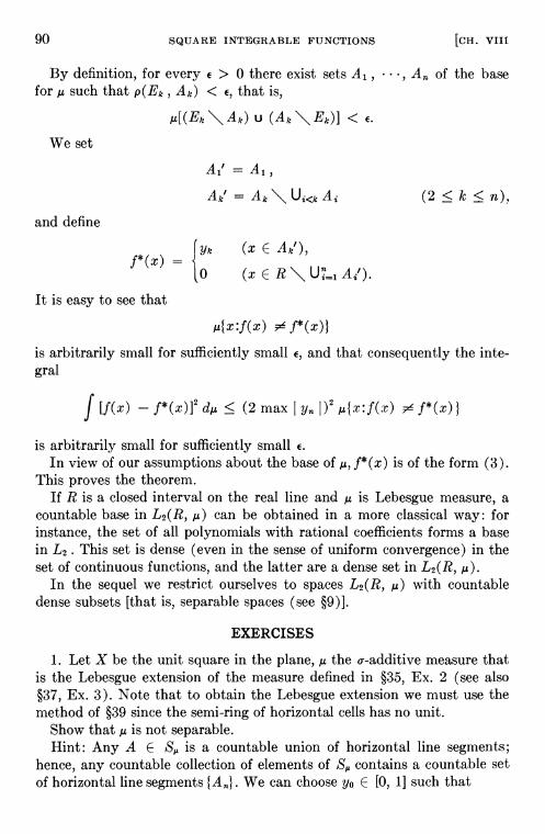
90 SQUARE INTEGRABLE FUNCTIONS {CH. VIII
By definition, for every 0 there exist sets A1, •••, of the basefor i2 such that p(Ek , < €, that is,
U (Ak\Ek)J <€.We set
,4F_ A!11 — tll ,
Ak' = (2 � k � n),and define
IYk (x E Ak'),f*(x) =(x E R \ A2').
It is easy to see that
is arbitrarily small for sufficiently small €, and that consequently the inte-gral
f [f(x) _f*(x)}2d/2 � (2 max I)2{:f()
is arbitrarily small for sufficiently small €.In view of our assumptions about the base of f*(x) is of the form (3).
This proves the theorem.If R is a closed interval on the real line and is Lebesgue measure, a
countable base in L2(R, /2) can be obtained in a more classical way: forinstance, the set of all polynomials with rational coefficients forms a basein L2. This set is dense (even in the sense of uniform convergence) in theset of continuous functions, and the latter are a dense set in L2(R, /2).
In the sequel we restrict ourselves to spaces L2(R, /2) with countabledense subsets [that is, separable spaces (see §9)].
EXERCISES
1. Let X be the unit square in the plane, the o-additive measure thatis the Lebesgue extension of the measure defined in §35, Ex. 2 (see also§37, Ex. 3). Note that to obtain the Lebesgue extension we must use themethod of §39 since the semi-ring of horizontal cells has no unit.
Show that is not separable.Hint: Any A E is a countable union of horizontal line segments;
hence, any countable collection of elements of contains a countable setof horizontal line segments We can choose yo E [0, 1] such that

§53] ORTHOGONAL SETS OF FUNCTIONS. ORTHOGONALIZATION 91
A0 = y):O � x 1, Y YoI
is disjoint from all these. Then show that
p(Ao, = /2(Ao � 1for all n.
2. a) Since 1i(R) < oc, a simp'e measurable function with onty finitelymany distinct values belongs to /2) for every p � 1.
b) The discussion in §51 can be paralleled for the present case to showthat every f E can be approximated in the mean of order p (i.e., inthe metric of by simple functions assuming only finitely many values.
c) The procedure of §52 can now be imitated to show that if has acountable base, then is separable for p � 1.
d) It follows from a) and c) that for r, s � 1, LT(R, is dense in LS(R, /2).
§53. Orthogonal sets of functions. Orthogonalization
In this section we consider functions f E L2 defined on a measurable setR with measure which we assume to have a countable base and to satisfythe condition /2(R) < oc. As before, we do not distinguish between equiva-lent functions.
DEFINITION 1. A set of functions
(1) çci(x),
is said to be linearly dependent if there exist constants e1 , • •, , not allzero, such that
(2) cicoi(x) + e2c02(x) + + cncon(x) = 0
a.e. on R. If, however, (2) implies that
(3) ci — = Cn = 0,
then the set (1) is said to be linearly independent.Clearly, a linearly independent set cannot contain functions equivalent
to&(x)DEFINITION 2. An infinite sequence of functions
(4) coi(x), • •, con(x),
is said to be linearly independent if every finite subset of (4) is linearlyindependent.
We denote by
M , )
the set of all finite linear combinations of functions of (4). This set is

92 SQUARE INTEGRABLE FUNCTIONS [CII. VIII
called the linear hull of (4) (or the linear manifold generated by {cokl). Welet
M , ...) M{cok}
denote the closure of M in L2. M is called the closed linear hull of (4) (orthe subspace generated by {cokl).
It is easily seen that M consists precisely of the functions f E L2 whichcan be approximated by finite linear combinations of functions of (4) witharbitrarily prescribed accuracy.
DEFINITION 3. The set of functions (4) is said to be complete (sometimesclosed) if
= L2.
Suppose that L2 contains a countable dense set of functions
fi,Deleting from this set those functions which are linearly dependent on thepreceding functions in the sequence, we obtain a linearly independent setof functions
gi,
which, as is easily seen, is complete.If L2 contains a finite complete set (1) of linearly independent functions,
then
L2 = , , con) M(coi, , con)
is isomorphic to Euclidean n-space. We say L2 is n-dimensional. Otherwise,we call L2 infinite-dimensional.
The space L2 is infinite-dimensional in all cases of interest in analysis.Obviously, in order that (4) be complete it is sufficient that it be possible
to approximate every function of a dense subset of L2 with arbitrary ac-curacy by linear combinations of functions of (4).
Let R = [a, b] be a closed interval on the real line with the usual Le-besgue measure. Then the set of functions
('5) x, x2,
is complete in L2(R, /2).For, according to the Weierstrass theorem (see Vol. 1, p. 25) the set of
linear combinations of functions (5) is dense in the set of all continuousfunctions. The completeness of the set (5) now follows from this remarkand Theorem 2, §51.
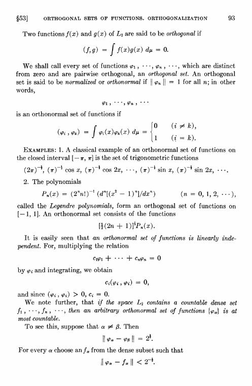
§53] ORTHOGONAL SETS OF FUNCTIONS. ORTHOGONALIZATION 93
Two functions f(x) and g(x) of L2 are said to be orthogonal if
(f,g) - f f(x)g(x) = 0.
We shall call every set of functions coi, , •, which are distinctfrom zero and are pairwise orthogonal, an orthogonal set. An orthogonalset is said to be normalized or orthonormal if = 1 for all n; in otherwords,
coi,
is an orthonormal set of functions if
a, 0cok) = J
1 (i=k).EXAMPLES: 1. A classical example of an orthonormal set of functions on
the closed interval [— ir, 7r] is the set of trigonometric functions
cos x, cos 2x, , sin x, sin 2x,
2. The polynomials
— (n 0, 1, 2, . .
called the Legendre polynomials, form an orthogonal set of functions on[— 1, 1]. An orthonormal set consists of the functions
+
It is easily seen that an orthonormal set of functions is linearly inde-pendent. For, multiplying the relation
Cicoi + ... + = 0
by and integrating, we obtain
0,
and since (cot, çoj) > 0, 0.We note further, that if the space L2 contains a countable dense set
11, • ••, then an arbitrary orthonormal set of functions {coa} is atmost countable.
To see this, suppose that a $. Then
— =
For every a choose an fa from the dense subset such that

94 SQUARE INTEGRABLE FUNCTIONS [CH. VIII
Clearly, fa i's if a Since the set of all fa is countable, the set ofis at most countable.
An orthonormal base is of great importance in studying finite-dimen-sional spaces. In this connection an orthonormal base is a set of orthogonalunit vectors, whose linear hull coincides with the whole space. In theinfinite-dimensional case the analogue of such a base is a complete ortho—normal set of functions, that is, a set
coi,
such that1) (pj,çok) ôik,2) M(coi , • ., , ) L2
We gave examples of orthonormal sets of functions on the intervals [— ir, 7r]
and [—1, 11 above. The existence of a complete orthonormal set of func-tions in an arbitrary separable space L2 is a consequence of the followingtheorem:
THEOREM. Suppose that the set of functions
(6) . .
is linearly independent. Then there exists a set of functions
(7)
satisfying the following conditions:1) The set (7) is orthonormal.2) Every function is a linear combination of the functions f', ,
+ + +with 0.
3) Every function is a linear combination of the functions
— + ... +
with 0.Every function of the set (7) is uniquely determined (except for sign) by
the Conditions 1 )—3).Proof. The function çoi(x) is uniquely determined (except for sign) by
the conditions of the theorem. For,
coi a11f1
(coi,
= a112(fi, fi) = 1,
whence
b11 = 1/au = (fi ,coi = ± (fi ,
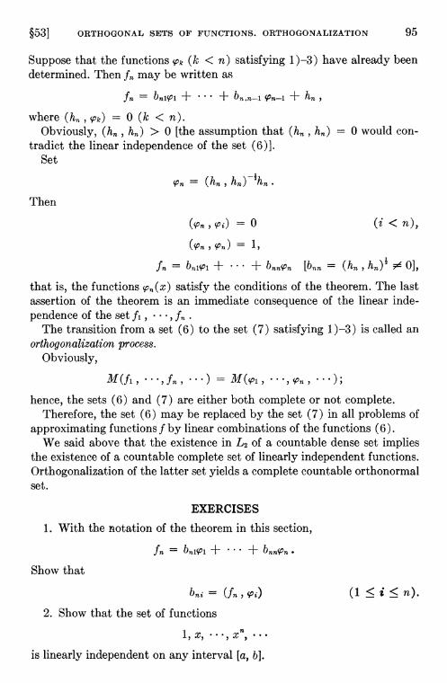
§53] ORTHOGONAL SETS OF FUNCTIONS. ORTHOGONALIZATION 95
Suppose that the functions (k < n) satisfying 1)—3) have already beendetermined. Then fTh may be written as
+ + con—i +
where , 00 [the assumption that (ha, 0 would con-
tradict the linear independence of the set (6)].Set
— (ha,
Then
0 (i < n),
, 1,
= + + , 0],
that is, the functions satisfy the conditions of the theorem. The lastassertion of the theorem is an immediate consequence of the linear inde-pendence of the set Ii, ,
The transition from a set (6) to the set (7) satisfying 1 )—3) is called anorthogonalization process.
Obviously,
M(f1, ...)hence, the sets (6) and (7) are either both complete or not complete.
Therefore, the set (6) may be replaced by the set (7) in all problems ofapproximating functions f by linear combinations of the functions (6).
We said above that the existence in L2 of a countable dense set impliesthe existence of a countable complete set of linearly independent functions.Orthogonalization of the latter set yields a complete countable orthonormalset.
EXERCISES
1. With the notation of the theorem in this section,
= + •.. +Show that
(fn,coj) (1
2. Show that the set of functions
1,x,
is linearly independent on any interval [a, b].

96 SQUARE INTEGRABLE FUNCTIONS [CH. VIII
3. For R = [0, 1] and /2 linear Lebesgue measure, show that L2(R,is infinite-dimensional.
4. Suppose that {fi(x), • . •, C L2. The Grammian of {f4 is thedeterminant
Show that is linearly dependent if, and only if, = 0. Hints: Suppose{ft} is linearly dependent. Multiply the dependency relation by(1 � i � n) and integrate to obtain a system of homogeneous equationswith a nontrivial solution. Conversely, if = 0, then the same systemhas a nontrivial solution a1, •••, Show that 0.
5. a) Show that the Legendre functions given in the text forman orthogonal set.
b) Show that + 1 Hint: is a polynomial ofdegree n. Use integration by parts repeatedly to show that is orthog-onal to (0 � k <n).
§54. Fourier series over orthogonal sets. The Riesz-Fisher theorem
If e2, e,, is an orthonormal base in Euclidean n-space thenevery vector x E can be written in the form
(1) x =
with
= (x, ek).
The purpose of this section is, in a sense, to generalize (1) to the infinite-dimensional case.
Let
(2) coi,
be an orthonormal set and suppose that f E L2.We pose the following problem: For prescribed n determine the coeffi-
cients ak (1 � k � n) so that the distance, in the sense of the metric inL2, between f and the sum
(3) Sn Ek=1 ak'pk
is the least possible.Set Ck = (f, Since the set (2) is orthonormal,
(4) II f — — , f — Ek=1
= (f, f) — 2(f, akcok) + ak'pk,
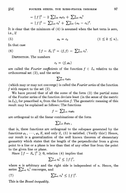
FOURIER SERIES. THE RIESZ-FISHER THEOREM 97
2 n n 2
II f II — 2 k=1 akck + k=1
2 n 2 n 2
= f — k=1 Cic + k=1 (ak — Ck)
It is clear that the minimum of (4) is assumed when the last term is zero,i.e., if
(5) ak—Ck (1�k<n).In that case
(6) = (f,f) —
DEFINITION. The numbers
Ck = (f,are called the Fourier coefficients of the function f E L2 relative to theorthonormal set (2), and the series
k=1
(which may or may not converge) is called the Fourier series of the functionf with respect to the set (2).
We have proved that of all the sums of the form (3) the partial sumsof the Fourier series of the function deviate least (in the sense of the metricin L2), for prescribed n, from the function f. The geometric meaning of thisresult may be explained as follows: The functions
f —
are orthogonal to all the linear combinations of the form
that is, these functions are orthogonal to the subspace generated by thefunctions , • •, if, and only if, (5) is satisfied. (Verify this!) Hence,our result is a generalization of the well known theorem of elementarygeometry which states that the length of the perpendicular from a givenpoint to a line or a plane is less than that of any other line from the pointto the given line or plane.
Since f — 12 � 0, relation (4) implies that
<where n is arbitrary and the right side is independent of n. Hence, theseries Ck2 converges, and
(7) Ek=lck < IfThis is the Bessel inequality.

98 SQUARE INTEGRABLE FUNCTIONS [CII. VIII
We introduce the following importantDEFINITION. An orthonormal set is said to be closed (sometimes com-
plete) if00 2 2(8) k=lck
f E L2. The relation (8) is called Parseval's equality.It is clear from (6) that the set (2) is closed if, and only if, the partial
sums of the Fourier series of every function f E L2 converge to f in themetric of L2 (that is, in the mean).
The notion of a closed orthonormal set is intimately related to the com-pleteness of a set of functions (see §53).
THEOREM 1. In L2 every complete orthonormal set is closed, and conversely.Proof. Suppose that is closed; then the sequence of partial sums
of the Fourier series of every f E L2 is mean convergent. Hence the linearcombinations of the elements of the set are dense in L2, that is,
is complete. Conversely, suppose that is complete, that is, thatevery f E L2 can be approximated with arbitrary accuracy (in the senseof the metric in L2) by linear combinations
of elements of the set then the partial sums
of the Fourier series off yield, in general, a still better approximation of f.Consequently, the series
k==1
converges to f in the mean, and Parseval's equality holds.In §53 we proved the existence of a complete orthonormal set in L2.
Inasmuch as closure and completeness are equivalent for orthonormal setsin L2, the existence of closed orthonormal sets in L2 need not be proved,and the examples of complete orthonormal sets in §53 are also examplesof closed sets.
Bessel's inequality (7) implies that in order that numbers c1, c2, ... bethe Fourier coefficients of a function f E L2 with respect to an orthonormalset it is necessary that the series
k=1 Ck
converge. In fact, this condition is not only necessary, but also sufficient.This result is stated in
THEOREM 2. (THE RIESZ-FISHER THEOREM.) Let be an arbitraryorthonormal set in L2, and let the numbers

§54] FOURIER SERIES. THE RIESZ-FISHER THEOREM 99
Cl, •••,Cn,
be such that the series2(9) k=lCk
converges. Then there exists a function f E L2 such that
ck — (f, cok),
k=lCk = (f,f.Proof. Set
=
Then
I — = + ... + c°n+p 12 ck.
Since the series (9) converges, it follows, in view of the completeness ofL2, that the sequence {fnl converges in the mean to a function f E L2.Furthermore,
(10) (fn,coi) + (f—fn,coi),
where the first term on the right is equal to c (n � i), and the second termapproaches zero as n oc, since
(f — fn , � Ill — fn I'll II.
The left side of (10) is independent of n; hence, passing to the limit asn oc, we obtain
(f, = c.Since, according to the definition of f(x),
(n—*oo),
it follows that
k=lck (f,f).This proves the theorem.
In conclusion, we prove the following useful theorem:THEOREM 3. In order that an orthonormal set of functions (2) be complete
it is necessary and sufficient that there not exist in L2 a function not equiva-lent to çb = 0 which is orthogonal to all the functions of (2).
Proof. Suppose that the set (2) is complete, and hence closed. If f E L2

100 SQUARE INTEGRABLE FUNCTIONS [CII. VIII
is orthogonal to all the functions of (2), then all its Fourier coefficients areequal to zero. Then Parseval's equality implies that
(f,f) = 0,
that is, f(x) is equivalent to 0.Conversely, suppose that is not complete, that is, there exists a
function g E L2 such that
(g, g) > Ck [Ck = (g, cok)].
Then, by the Riesz-Fisher theorem, there exists a function f E L2 such that
(f, = Ck, (f, 1)
The function f — g is orthogonal to all the functions coi.. In view of theinequality
(f, f) = Ck2 < (g, g),
f — g cannot be equivalent to 4'(x) = 0. This proves the theorem.
EXERCISES
1. Let be an orthonormal set in L2 and suppose f E L2. Verifythat f — is orthogonal to all linear combinations if,and only if, ak (1, (1 � k n).
2. Let be an orthonormal set in L2 and let F L2 be dense inL2. If Parseval's equality holds for each f E F, then it holds for all g E L2,i.e., {ccn(x)1 is closed.
This may be proved as follows: Let be the nthpartial sum of the Fourier series of f E L2.
a) 1ff, g E L2, then
— = II — If — g II.
b) Parseval's equality holds for g if, and only if,
II g — sn(g) II = 0.
c) Now use the hypothesis of the exercise.3. Let be complete orthonormal sets in L2(R, /2). Let
/2 /2 and consider L2(R X R,a) The set { Xnm(X, y) :n, m = 1, 2, •} is orthonormal
in L2(R x R, 2)
b) The set { Xnm(X, y) } is complete.Hint: Use Fubini's theorem and the criterion of Theorem 3 for complete-ness.
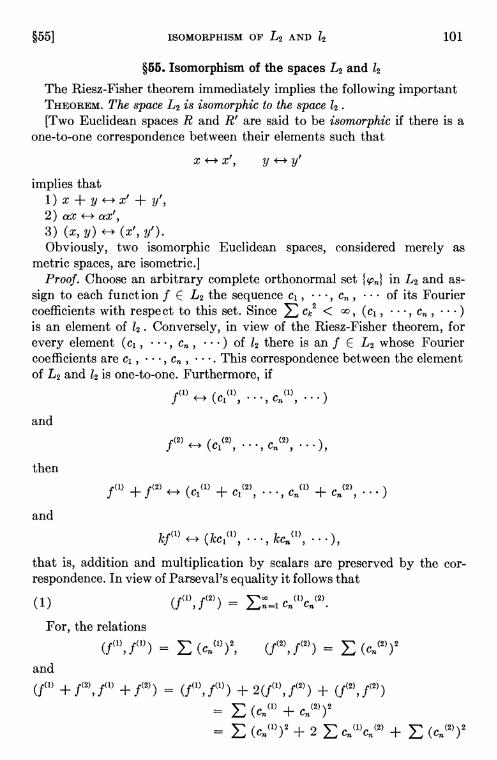
§551 ISOMORPHISM OF L2 AND 12 101
§55. Isomorphism of the spaces L2 and 12
The Riesz-Fisher theorem immediately implies the following importantTHEOREM. The space L2 is isomorphic to the space 12.[Two Euclidean spaces R and R' are said to be isomorphic if there is a
one-to-one correspondence between their elements such that
y<—*y'
implies that1) x + y x' + y',2) ax ax',3) (x, y) (x', y').Obviously, two isomorphic Euclidean spaces, considered merely as
metric spaces, are isometric.]Proof. Choose an arbitrary complete orthonormal set in L2 and as-
sign to each funct ion f E L2 the sequence c1, •••, ... of its Fouriercoefficients with respect to this set. Since < (c1, •, , •
is an element of 12. Conversely, in view of the Riesz-Fisher theorem, forevery element (c1, •..) of 12 there is an f E L2 whose Fouriercoefficients are c1, •'•, •••. This correspondence between the elementof L2 and 12 is one-to-one. Furthermore, if
••')and
f(2) •••, •..),then
f(2)—1— • • •, —I--• • • • )
and
7.e(1) (1) (1), ••, ,
that is, addition and multiplication by scalars are preserved by the cor-respondence. In view of Parseval's equality it follows that/1 \ e(2)\ 00 (1) (2)
,J ) — n=1
For, the relationsf(l)) = (f(2), f(2) =
and(f(1) f(2) f(l) f(2)) (f(l) fW) f(2)) (f(2), f(2))
= += + 2 +

102 SQUARE INTEGRABLE FUNCTIONS [CH. VIII
imply (1). Hence the above correspondence between the elements of L2and 12 is an isomorphism. This proves the theorem.
On the basis of this theorem we may regard 12 as a "coordinate form"of L2. It enables us to carry over to L2 results previously established for12. For instance, we proved in Chapter III that every linear functional in12 is of the form
ço(x) (x,y),
where y is an element of 12 uniquely determined by the functional ço. Inview of this and the isomorphism between L2 and 12, it follows that everyfunctional in L2 is of the form
= (f,g) = f f(x)g(x)
where g(x) is a fixed function of L2. We proved in §24 that 12 = 12. HenceL2 = L2.
The isomorphism between L2 and 12 established above is closely relatedto the theory of quantum mechanics. Quantum mechanics originallysisted of two superficially distinct theories: Heisenberg's matrix mechanicsand Schrodinger's wave mechanics. Schrodinger later showed that thesetwo theories are equivalent. From the mathematical point of view, thedifference between the two theories reduced to the fact that the Heisen-berg theory used the space 12, while the Schrodinger theory used the spaceL2.
EXERCISES
1. Let be an orthonormal set in L2. Then nonequivalent func-tions f, g have distinct Fourier series, i.e., for some n, (f, çcn) (g, ccn)if, and only if, is complete. This result justifies the statement in thetext that f (ci, c2, •, .) is a one-to-one correspondence. Hint:Apply Theorem 3 of §54.
2. Let be a complete orthonormal set in L2(R, /1) and supposef E L2.The Fourier series of f(x) can be integrated term by term over an arbi-trary measurable subset A of R, i.e.,
ff(x) d/2 = ckf
where Ck = (f, is the kth Fourier coefficient of f(x).Hint: Let fW = f, f(2) = XA in equation (1) of the theorem of this sec-
tion.
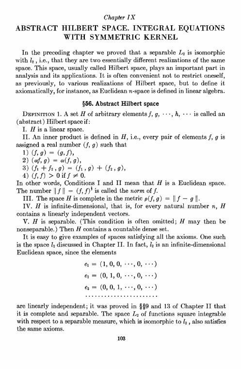
IX
ABSTRACT HILBERT SPACE. INTEGRAL EQUATIONSWITH SYMMETRIC KERNEL
In the preceding chapter we proved that a separable L2 is isomorphicwith 12, i.e., that they are two essentially different realizations of the samespace. This space, usually called Hilbert space, plays an important part inanalysis and its applications. It is often convenient not to restrict oneself,as previously, to various realizations of Hilbert space, but to define itaxiomatically, for instance, as Euclidean n-space is defined in linear algebra.
§56. Abstract Hubert space
DEFINITIoN 1. A set H of arbitrary elements f, g, •••, h, is called an(abstract) Hubert space if:
I. H is a linear space.II. An inner product is defined in H, i.e., every pair of elements f, g is
assigned a real number (f, g) such that1) (f,g) = (g,f),2) (af,g) = a(f,g),3) (fi+f2,g) = (fi,g) + (f2,g),4) (f,f) > Oiff 0.
In other words, Conditions I and II mean that H is a Euclidean space.The number f = (f, is called the norm of f.
III. The space H is complete in the metric p(f, g) = f — g J.
IV. H is infinite-dimensional, that is, for every natural number n, Hcontains n linearly independent vectors.
V. H is separable. (This condition is often omitted; H may then benonseparable.) Then H contains a countable dense set.
It is easy to give examples of spaces satisfying all the axioms. One suchis the space 12 discussed in Chapter II. In fact, 12 is an infinite-dimensionalEuclidean space, since the elements
e1 = (1, 0, 0, . , 0, )
e2 = (0, 1, 0, • • •, 0, • • )
e3 = (0, 0, 1, • , 0, • )
are linearly independent; it was proved in and 13 of Chapter II thatit is complete and separable. The space L2 of functions square integrablewith respect to a separable measure, which is isomorphic to 12, also satisfiesthe same axioms.
103

104 ABSTRACT HILBERT SPACE. INTEGRAL EQUATIONS [CH. IX
The following proposition holds:All Hubert spaces are isomorphic.To prove this, it is obviously sufficient to show that every Hubert space
is isomorphic to the coordinate space 12. The latter assertion is proved byessentially the same arguments as were used in the proof of the isomorphismof L2 and 12
1. The definitions of orthogonality, closure and completeness, whichwere introduced in §53 for elements of L2, can be transferred unchangedto abstract filbert space.
2. Choosing in H a countable dense set and applying to it the process oforthogonalization described (for L2) in §53, we construct in H a completeorthonormal set, that is, a set
(1) h1,
satisfying:a)
10(hi, hk) = (i=k).
b) The linear combinations of the elements of (1) are dense in H.3. Let f be an arbitrary element of H. Set Ck = (f, hid). Then the series
Ck2 converges, and Ck2 (f, f) for an arbitrary complete orthonormalset andf E H.
4. Suppose again that {hkl is a complete orthonormal set in H. If
c1,
is a sequence of numbers such that
<
there exists an f E H such that
= (f, hk),
and
= (ff)5. It is clear from what we have said that an isomorphism between H
and 12 can be realized by setting
f •.'),where
ck = (f, hk)

§56] ABSTRACT fILBERT SPACE 105
and
h1,h2,
is an arbitrary complete orthonormal set in H.The reader may carry out the details of the proof as in
EXERCISES
1. a) The norm f in H satisfies the parallelogram law:
1 + + 1— f2 12 = 2( + H f2 12).
b) Conversely, if X is a complete separable normed linear space inwhich the norm satisfies the parallelogram law, then an inner product maybe defined in X by
1 2 2
(f, g) = H f + g H — If— g H].
Moreover, (f, f) = H 1 and X becomes a Hilbert space. Hints: (i) Es-tablish first that (x, y) is a continuous function of x. (ii) Show by induc-tion that (nx, y) = n(x, y). Itwill then readilyfollow that (ax, y) = a(x, y).(iii) Then establish that (xi + x2, y) = (xi, y) + (x2, y). The otherproperties of an inner product are immediate.
2. Suppose that A H has the property that f, g E A implies that+ g) E A (this is true, in particular, if A is convex). Let
d inf{ :f E A}.
If {f7j c A has the property that H = d, show that {f7j is afundamental sequence in H.
Since H is complete, it follows that f exists in H. If A isclosed, thenf E A.
Hint: The parallelogram law yields
4' \ 2 _L4' 2
2kjn Jm) — 2 Jn F 2 Jm 2'Jn FJm)
3. In Def. 2 of §50 it is stated that the Schwarz inequality:
(f g)2 � H f g 12
holds. The author proves Schwarz's inequality in several concrete cases(see vol. 1, pp. 17, 18). Prove that the inequality holds in H (only AxiomsI and II of §56 are required).
Hint: Suppose that f, g E H and that t is real. The quadratic polynomialwith real coefficients in t: (f + t(f, g)g, f + t(f, g)g) is nonnegative; hence,its discriminant must be nonpositive.

106 ABSTRACT HILBERT SPACE. INTEGRAL EQUATIONS [cH. IX
4. The inner product (f, g) is a continuous function of f and g, i.e., ifH f 1
—÷0 and — g —÷0 for f, g in H, then gn)(f,g).
5. The following is an example of a nonseparable Hubert space. Let Hbe the collection of all real-valued functions defined on [0, 1] with f(x) 0for only countably many x E [0, 1], and such that if 0 forthen < The addition of functions and multiplication byreal numbers is defined in the usual way, i.e., pointwise.
a) Define (f, g) analogously to the scalar product in 12 and showthat H satisfies I, II, III, IV in Def. 1.
b) Show that H is not separable. Hint: Show that H contains un-countably many disjoint open spheres.
6. II in the preceding example we restrict the collection H further tothose f(x) whose values are not zero for only finitely many x, then withthe same operations H is also an incomplete metric space. That is, find afundamental sequence in H whose limit is not in H. Note that the limitof such a sequence will be an element of H in Ex. 5.
§57. Subspaces. Orthogonal complements. Direct sums
In accordance with the general definitions of Chapter III, §21, a linearmanifold in H is a subset L of H such that if f, g E L, then af + E Lfor arbitrary numbers a and A subspace of H is a closed linear manifoldin H.
We give several examples of subspaces of H.1. Suppose that h E H is arbitrary. The set of all f E H orthogonal to
h is a subspace of H.2. Let H = 12, that is, all the elements of H are sequences
(x1,
of numbers such that Xk2 < The elements satisfying the condition= x2 form a subspace.3. Let H be the space L2 of all square summable functions on a closed
interval [a, b] and suppose that a < c < b. We denote byH identically zero on [a, c]. is a subspace of H. If
C1 < C2, then and Ha = H, Hb = (0). Hence we obtain acontinuum of subspaces of H ordered by inclusion. Each of these subspaces(with the exception, of course, of Hb) is infinite-dimensional and isomorphicto H.
The verification of the fact that each of the sets described in 1—3 isindeed a subspace of H is left to the reader.
Every subspace of a Hilbert space is either a finite-dimensional Euclideanspace or itself a Hilbert space. For, Axioms I—Ill are obviously satisfiedby a subspace and the validity of Axiom V follows from the following lemma:

§57J SUBSPACES. ORTHOGONAL COMPLEMENTS. DIRECT SUMS 107
LEMMA. If a metric space R contains a countable dense 8et, every 8ubspaceR' of R contains a countable dense set.
Proof. [TRANS. NOTE. The proof in the original was incorrect. We havetherefore substituted the following proof.]
We assume that R' 0, otherwise there is nothing to prove.Let { be dense in R. For every pair of natural numbers n, k choose a
E R' (if it exists) such that
< 1/2k.
Then ; n, k = 1, 2, . . '1 is dense in R'. To see this, suppose that x E R'and e > 0. Choose an s such that 1/s < Since is dense in R andx E R, there is an m such that p(Em, x) < 1/2s. Hence exists and
p(x, vms) � p(X, Em) + P(Em, vms) < 1/2s + 1/28 = 1/8 <f.The existence in Hubert space of an inner product and the notion of
orthogonality enable us to supplement substantially the results of Vol. 1 onsubspaces of arbitrary Banach spaces.
By orthogonalizing a countable dense sequence of elements of an arbi-trary subspace of a Hubert space, we obtain
THEOREM 1. Every subspace M of H contains an orthogonal set whoselinear closure coincides with M:
M = M(cei,
Let M be a subspace of H. Denote by
M'—HeMthe set of g E H orthogonal to all f E M. We shall prove that M' is alsoa subspace of H. The linearity of M' is obvious, since , f) = , f) = 0implies that (aigi + a2g2 , f) = 0. To prove closure, suppose that gn E M'and that gn converges to g. Then
(g, f) = , f) = 0
for all f E M, and consequently g E M'.M' is called the orthogonal complement of M.From Theorem 1 it easily follows that:THEOREM 2. If M is a 8ub8pace of H, every f E H is uniquely representable
in the form f = h + h', where h E M, h' E M'.Proof. We shall first prove the existence of the decomposition. To this
end, we choose in M a complete orthonormal set such that M =and set
h = = (f, çe'1j.
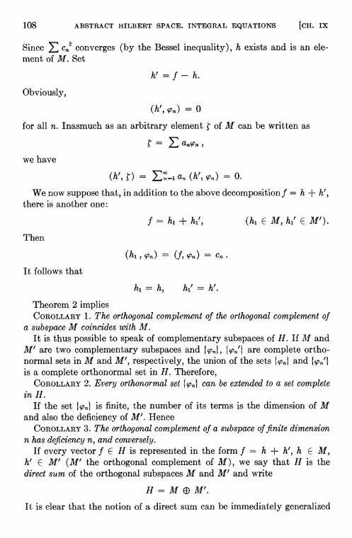
108 ABSTRACT HILBERT SPACE. INTEGRAL EQUATIONS [CH. IX
Since converges (by the Bessel inequality), h exists and is an ele-ment of M. Set
h' = f — h.
Obviously,
(h', = 0
for all n. Inasmuch as an arbitrary element of M can be written as
we have
= = 0.
We now suppose that, in addition to the above decomposition f = h + h',there is another one:
f = + h1', (h1 E M, h1' E M').
Then
(h1, = (f, =
It follows that
h1 = h, h1' = h'.
Theorem 2 impliesCOROLLARY 1. The orthogonal complement of the orthogonal complement of
a subspace M coincides with M.It is thus possible to speak of complementary subspaces of H. If M and
are two complementary subspaces and are complete ortho-normal sets in M and M', respectively, the union of the sets andis a complete orthonormal set in H. Therefore,
COROLLARY 2. Every orthonormal set can be extended to a set completein H.
If the set is finite, the number of its terms is the dimension of Mand also the deficiency of M'. Hence
COROLLARY 3. The orthogonal complement of a subspace of finite dimensionn has deficiency n, and conversely.
If every vector f E H is represented in the form f = h + h', h E M,h' E M' (M' the orthogonal complement of M), we say that H is thedirect sum of the orthogonal subspaces M and M' and write
H=MEJ?M'.It is clear that the notion of a direct sum can be immediately generalized

§57] SUBSPACES.. ORTHOGONAL COMPLEMENTS. DIRECT SUMS 109
to an arbitrary finite or even countable number of subspaces: H is thedirect sum of subspaces M1, ••• ,
H M1 El? El? E13
if1) the subspaces are pairwise orthogonal, that is, an arbitrary vector
in M is orthogonal to an arbitrary vector in Mk (i k);2) every f E H can be written in the form
(1) f=h1+•••where 12 converges if the number of subspaces is infinite.
It is easily verified that the sum (1) is unique and that
If 112 = II12
A notion related to the direct sum of subspaces is that of the direct sumof a finite or countable number of arbitrary Hubert spaces. If H1, H2 areHubert spaces, their direct sum H is defined as follows: the elements of Hare all possible pairs (h1, h2), where h1 E H1, h2 E H2, and the innerproduct of two such pairs is
1/1.. L\ IL, — IL I IL112), , Ft2 ) I — '11 ) 1 ,
The space H obviously contains the orthogonal subspaces consisting ofpairs of the form (h1 , 0) and (0, h2), respectively; the first can be identi-fied in a natural way with the space H1, and the second with H2.
The sum of an arbitrary finite number of spaces is defined in the sameway. The sum H of a countable number of spacesH1, , is defined as follows: the elements of H are all possiblesequences of the form
such that
The inner product (h, g) of h, g E H is equal to
(ha, gn).
EXERCISES
1. Prove Corollary 1 of Theorem 2.2. Prove the remark before Corollary 2: If M, M' are complementary
subspaces and if are complete orthonormal sets in M, M', re-spectively, then their union is a complete orthonormal set in H.

ABSTRACT HILBERT SPACE. INTEGRAL EQUATIONS [CH. IX
3. If M, N are orthogonal subspaces, then
M+N = {f+g:fE M,g E NIis closed, and therefore a subspace. If M, N are not orthogonal, the resultneed not be true. (An example can be found in Halmos, P. R., Introductionto Hubert Space and the Theory of Spectral Multiplicity, New York, 1951.)
Hint: It is enough to show that if + is a fundamental sequence,then and are also fundamental.
It is the purpose of the following exercises to extend some of the resultsof the text to general (i.e., nonseparable) Hilbert spaces.
4. If a subspace M of H is proper, i.e., H \ M 0, then there exists anelement g of H, g 0, such that g is orthogonal to every element of M.
Hint: For h E H \ M, h — M = {h — x : x E is closed and convex.Letd = inf h — x II:x E d = h — x0 x0 E M (see §56, Ex. 2).For arbitrary real c and f E M, show that
0 � h — (Xo + cf) — h —
Show that this holds only if g = h — x0 is orthogonal to M. g will be therequired element.
5. If M, N are subspaces of H, N M, then we denote by M e N theorthogonal complement of N in M (consider M itself as a Hilbert space).Show that M = N (M e N).
Hint: Let L = N (M e N), with L M and L closed (see Ex.3). If L is properly contained in M, apply the result of Ex. 4 to obtain acontradiction.
6. Let F(f) be a bounded linear functional on H. There exists one andonly one element g in H such that F(f) = (f, g) for every f in H [comparewith equation (1) at the beginning of the next section].
a) The uniqueness is easy to establish.b) LetM = = O}. Misa subspace. IfM = H, chooseg = 0.
Otherwise, by Ex. 4 there exists an h 0 such that h is orthogonal to M.Show that g = [F(h)/(h, h)]h will do.
§58. Linear and bilinear functionals in Hubert space
The isomorphism of every Hilbert space with 12 enables us to carry overto an abstract Hilbert space the results established in Chapter III for 12.
Since every linear functional in 12 is of the form
ço(x) = (x, a) (a E 12),
it follows that:An arbitrary linear functional F(h) in H is of the form
(1) F(h) = (h, g),
where g depends only on F.

§58] LINEAR AND BILINEAR FIJNCTIONALS 111
Hence, the definition of weak convergence introduced in Chapter IIIfor an arbitrary linear space, when applied to H can be stated in the fol-lowing way:
A sequence hn E H is weakly convergent to h E H if1) the norms II II are bounded (see p. 90 of vol. 1);2) for every g E H,
(hn, g) —÷ (h, g).
Ex. 4 at the end of the section shows that 2) implies 1).An arbitrary orthonormal sequence
'P1, •••
in H converges weakly to zero, since
en = (n—f oo)
for arbitrary h E H, in view of the fact that
ECn2� (/i,/i) <Such a sequence, of course, does not converge in the norm.
In particular, applying these remarks to the case when H is the space ofsquare integrable functions on a closed interval [a, b] of the real line withthe usual Lebesgue measure, we obtain the following interesting result:Let
,
be an orthonormal set of functions in H, and let
f(t) — 1 (on [ti, t2} c [a, b]),
— 0 (outside [t1, t2]).
Then
(f, = J dt.tl
Hencert2
JLi
for an arbitrary orthonormal set of functions con(t) and arbitrary ti,12 E [a, b].
If the are uniformly bounded,b
f ço(t) dt = 1

112 ABSTRACT HILBERT SPACE. INTEGRAL EQUATIONS [CH. IX
only if the number of sign changes of on [a, b] is unbounded as n(the same is to be observed, for instance, in the case of trigonometricfunctions).
In Chapter III, parallel with the concept of weak convergence of theelements of a linear normed space, we introduced the notion of weak con-vergence of a sequence of functionals. Inasmuch as Hubert space coincideswith its conjugate space, these two types of convergence are identical.Therefore, Theorem 1' of §28 yields the following result for Hubert space H:
The unit sphere in H is weakly compact, that is, every sequence E H,with 1, contains a weakly convergent subsequence.
In the sequel we require in addition the followingTHEOREM 1. If is weakly conifergent to in H, then
Proof. For every complete orthonormal set in H,
ck = Wk) = , (Pk) =
= < SUPn cnm2;
consequently,
cm2 � supn
which proves the theorem.Let B(f, g) be a real-valued function of pairs of elements of H satisfying
the following condition: B(f, g) is a linear functional off for fixed g, and alinear functional of g for fixed f. B(f, g) is called a bilinear functional.A bilinear functional B(f, g) is said to be symmetric if
B(f,g) = B(g,f) (f,g E H).
The theorem on the general form of a linear functional in H implies thatevery bilinear functional in H can be written in the form
B(f, g) = U•, g),
where depends on f. It is easily seen that the correspondence
is a continuous linear operator in H; denote it by A. Hence
(2) B(f, g) = (Af, g).
An alternative form
B(f, g) = (f, A*g',

§58} LINEAR AND BILINEAR FTJNCTIONALS 113
where A* is the adjoint operator of A, can be obtained in a similar fashion.[In Chapter III, in considering linear operators on an arbitrary Banachspace B, we defined the adj oint operator A * of A by means of the relation
(Ax, cc) = (x, A*W) (x E B, E E).
If B is a Hilbert space, then E = B, and the definition of A* in Chapter IIIreduces to the definition given above.] If a functional B(f, g) is symmetric,then
(Af,g) = B(f,g) = B(g,f) = (Ag,f) = (f,Ag),
that is,
(3) A=A*.A linear operator satisfying (3) is said to be self -adjo'int.Formula (2) defines a one-to-one correspondence between the bilinear
functionals and the continuous linear operators on H, with the symmetricbilinear functionals corresponding to the self-adjoint linear operators, andconversely.
Setting f = g in a symmetric bilinear functional, we obtain a quadraticfunctional
Q(f) = B(f,f).According to (2),
Q(f) = (Af,f),where A is a self-adjoint linear operator.
Since the correspondence between the symmetric bilinear functionals andthe quadratic functionals is one-to-one [Q(f) = B(f, f), and conversely:B(f, g) = + g) — Q(f — g)}], the correspondence between thequadratic functionals and the seif-adjoint linear operators is also one-to-one.
EXERCISES
1. Let M be a proper subspace of H, F(h) a (bounded) linear functionalon M with norm F Then there exists a linear functional F* on H suchthat F*(h) = F(h) for h E M and F (See vol. 1, p. 86, theHahn-Banach theorem.) Hint: Apply equation (1) at the beginning of thissection to the Hubert space M.
2. a) Let and f(x) belong to H. If converges strongly to f,then converges weakly to f.
b) The converse is false. Show that for L2(R, where R = [0, 1]
and is linear Lebesgue measure, that { sin nx} is weakly convergent to

ABSTRACT HILBERT SPACE. INTEGRAL EQIJATIONS [CH. IX
f(x) = 0, but {sin nx} is not fundamental in the norm; hence it cannotconverge strongly to any element of L2.
c) The following partial converse is true. If converges weakly tof and converges to f then converges strongly to f. Hint:Show that (f — f — 0.
3. Suppose A H. If A is weakly closed, then A is a norm closed subsetof H. More explicitly: Suppose A and (f, g)g f E that f A impliesfEA.
4. The definition of weak convergence of to h in H lists two condi-tions. We propose to show that the second condition already implies thefirst. This result in a more general setting is known as the Banach-Stein-haus theorem.
a) It is enough to show that there exists a constant M > 0 and asphere S = g — go II � r} such that g E S implies
I, g)
IM.
For if this implication holds and g1� r, then
I I
= + go) — <2M.
Now show that g E H implies
I� (2M/r)
I� 2M/r.
b) It follows that if the result is false, the sequence {I
, g) mustbe unbounded in every sphere, i.e., given a > 0 and S a sphere in H,there is an element ga E S and an index fla for which
I I> a.
Show by continuity of (h, g) in the second argument that S contains aclosed sphere Sa such that g E Sa implies I g) > a.
c) Now construct by induction a sequence of closed spheres { &}and a sequence {flk} such that Sk Sk-1 ; diam Sk < 1/k; n1 <n2 < •.•flk < ; and (hflk, g) > k for g E Sk.
d) Use the completeness of the metric space H to show the existenceof a point go for which I go) > k. This contradicts Condition 2):
, go) (h, go).5. Let M1 and M2 be two subspaces with M1 a proper subset of M2.
Show that there exists an element g of M2 such that g = 1 andII g — I II � 1 for any f E M1. Hint: Consider M2 as a Hilbert space withsubspace M1.
6. a) Let X be a Banach space, M a subspace of X and = M + x ={y + x : y E M} a subset of X defined for each x E X. We can make thecollection : x E = X/M into a vector space, called the quotient space

§59] COMPLETELY CONTINUOUS SELF-ADJOINT LINEAR OPERATORS 115
of X mod M by defining + = {M + (x + y)} and = {M + ax}.Verify that the operations are uniquely defined and that X/M is a vectorspace with zero element = M.
b) A norm is introduced by defining
Show that X/M is a normed linear space. The fact that M is closed isrequired to show that = 0 if, and only if, = ii
c) it is also true that X/M is complete, i.e., X/M is a Banach space.This is more difficult to prove.
7. If X = H and M is a subspace of H, show that H/M and H e M areisomorphic normed vector spaces. In other words, suppose that f E H,f = h + h', with h E M, h' E M'. Suppose that f corresponds to h' andshow that this correspondence is one-to-one, onto and preserves addition,multiplication by scalars, and the norm. Hint: I H2 = h 112 + II h' 112.
§59. Completely continuous seif-adjoint operators in H
In Chapter IV we introduced the notion of a completely continuouslinear operator, acting on a Banach space E. In this section we restrictthe discussion to self-adj oint completely continuous operators acting on aHilbert space, supplemented by the results already established for arbi-trary completely continuous operators.
We recall that we called an operator A completely continuous if itmapped every bounded set into a compact set. Inasmuch as H = 17, thatis, H is conjugate to a separable space, the bounded sets in H are preciselythe weakly compact sets (see Ex. 1 at the end of the section). Therefore,the definition of a completely continuous operator on a filbert space canbe stated as follows:
An operator A acting on a Hilbert space H is said to be completely con-tinuous if it maps every weakly compact set into a compact set (relative tothe norm).
In a Hilbert space this is equivalent to the condition that the operator Amap every weakly convergent sequence into a norm convergent sequence(see Ex. 2 at the end of the section).
In this section we shall prove the following fundamental theorem, ageneralization to completely continuous operators of the theorem on thereduction of the matrix of a self-adjoint linear transformation in n-dimen-sional space to diagonal form:
THEOREM 1. For every completely continuous self-adjo'int linear operator Aon a Hilbert space H there exists an orthonormal set of eigenvectors (characteris-tic vectors; see vol. 1, p. 110) corresponding to eigenvalues (characteristic

116 ABSTRACT HILBERT SPACE. INTEGRAL EQUATIONS [CH. IX
values){
such that every E H can be written uniquely in the form =+ E', where the vector satisfies the condition = 0. Also
= Ek Xkckcok,
and = 0.
For the proof of this fundamental theorem we require the followinglemmas:
LEMMA 1. If { converges weakly to and the self-adjoint linear operatorA is completely continuous, then
= (As, —> (As, =
Proof.
I
— (Au) — + — (Au) I.
But
— = I — I II 1111 —
and
I(As, — (As,
I = I — —
Since the numbersH
are bounded and A — 0,
I— —>0.
This proves the lemma.LEMMA 2. If a functional
I I I,
where A is a bounded self-adjoint linear operator, assumes a maximum at apoint of the unit sphere, then
'1) = 0
implies that
= (Eo,An) = 0.
Proof. Obviously, lEo = 1. Set
= +a is an arbitrary number. From = 1 it follows that
EM = 1.
Since
= (1 + a21 n + +

§59] COMPLETELY CONTINUOUS SELF-ADJOINT LINEAR OPERATORS 117
it follows that
= + + O(a2)
for small values of a. It is clear from the last relation that if (A 0,then a can be chosen so that >
I . This contradicts thehypothesis of the lemma.
It follows immediately from Lemma 2 that if I I assumes a maximumat = then is an eigenvector of the operator A.
Proof of the theorem. We shall construct the elements cok by induction, inthe order of decreasing absolute values of the corresponding eigenvalues:
To construct the element we consider the expression = I (As,and show that it assumes a maximum on the unit sphere. Let
S = sup
and suppose that is a sequence such that II 1 � 1 and
Since the unit sphere in H is weakly compact, { contains a subsequenceweakly convergent to an element In view of Theorem 1, §58,
II � 1,
and by Lemma 1,
I(An, = S.
We take as ce'i. Clearly, II I! = 1. Also
=
whence
Xii = I I(Açci,çoi) = S.
Now suppose that the eigenvectors
••• ,(Pn
corresponding to the eigenvalues
xl, •.. ,Xfl
have already been constructed. We consider the functional
on the elements of
= H e , , pn)

118 ABSTRACT HILBERT SPACE. INTEGRAL EQUATIONS [CH. IX
(that is, the set orthogonal to , and such that I! Ii � 1.
is an invariant subspace (a subspace which is mapped into itself) of A[since M(çoi, , is invariant and A is self-adjoint]. Applying theabove arguments to we obtain an eigenvector Wn+1 of A in Ma'.
Two cases are possible: 1) after a finite number of steps we obtain asubspace in which (As, = 0; 2) (As, 0 on for all n.
In the first case Lemma 2 implies that A maps into zero, that is,consists of the eigenvectors corresponding to X = 0. The set of vec-
tors is finite.In the second case we obtain a sequence {con} of eigenvectors for each of
which 0. We show that 0. The sequence (like every ortho-normal sequence) is weakly convergent to zero. Therefore, =converge to zero in the norm, whence =
1
0.
Let
M' = 0.
If E M' and E 0, then
(AE,
for all n, that is,
(As, = 0.
Hence, applying Lemma 2 (for sup {I
(As, I; 1
1} = 0) to M', weobtain A maps the subspace M' into zero.
From the construction of the set tcon} it is clear that every vector can bewritten in the form
= Eic Ckcok + (As' = 0).
Hence
A be a continuous linear operator of H into H. Suppose thatc H, f E H and converges weakly to f. Show that converges
weakly to Af.2. In the second paragraph of this section it is stated that in H the norm
bounded sets are precisely the weakly compact sets. Show that this is trueas follows:
a) If A H is norm bounded, i.e., there exists an M > 0 such thatIf II < M for allf E A, then Theorem l'of §28 (see vol. 1) shows that A
is weakly compact (see the statement preceding Theorem 1 in §58).
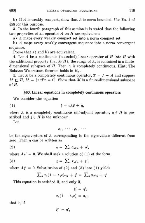
§60] LINEAR OPERATOR EQUATIONS 119
b) If A is weakly compact, show that A is norm bounded. Use Ex. 4 of
§58 for this purpose.3. In the fourth paragraph of this section it is stated that the following
two properties of an operator A on H are equivalent:a) A maps every weakly compact set into a norm compact set.b) A maps every weakly convergent sequence into a norm convergent
sequence.Prove that a) and b) are equivalent.4. Let A be a continuous (bounded) linear operator of H into H with
the additional property that A (H), the range of A, is contained in a finite-dimensional subspace of H. Then A is completely continuous. Hint: TheBolzano-Weierstrass theorem holds in
5. Let A be a completely continuous operator, T = I — A and supposeH, M = {x: Tx = 0}. Show that M is a finite-dimensional subspace
of H.
§60. Linear equations in completely continuous operators
We consider the equation
(1)
where A is a completely continuous self-adjoint operator, E H is pre-scribed and E H is the unknown.
Let
'P1,
be the eigenvectors of A corresponding to the eigenvalues different fromzero. Then can be written as
(2) = + n',where = 0. We shall seek a solution of (1) of the form
(3) = +where A E' = 0. Substitution of (2) and (3) into (1) yields
— + = +This equation is satisfied if, and only if,
= '1',
— =
that is, if
= 77',
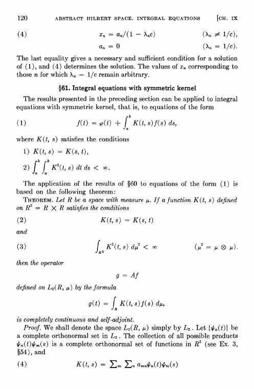
120 ABSTRACT HILBERT SPACE. INTEGRAL EQUATIONS [CH. IX
(4) = — 1/c),
= 0 = 1/c).
The last equality gives a necessary and sufficient condition for a solutionof (1), and (4) determines the solution. The values of corresponding tothose n for which = 1/c remain arbitrary.
§61. Integral equations with symmetric kernel
The results presented in the preceding section can be applied to integralequations with symmetric kernel, that is, to equations of the form
(1) f(t) = +f K(t, s)f(s) ds,
where K(t, s) satisfies the conditions
1) K(t, s) = K(s, t),
2) f1b
K2(t, s) dt ds < oc.
The application of the results of §60 to equations of the form (1) isbased on the following theorem:
THEOREM. Let R be a space with measure If a function K(t, s) definedon R2 = R X R satisfies the conditions
(2) K(t, s) = K(s, t)
(3) f K2(t, s) < oc (M2 = ®
then the operator
g = Af
defined on L2(R, by the formula
g(t) = f K(t, s)f(s) dM3
is completely continuous and seif-adjoint.Proof. We shall denote the space L2(R, simply by L2. Let be
a complete orthonormal set in L2. The collection of all possible products/'n(t)/'m(5) is a complete orthonormal set of functions in R2 (see Ex. 3,§54), and
(4) K(t, s) = Em amn/'n(t)/'m(s)

§611 INTEGRAL EQUATIONS WITH SYMMETRIC KERNEL 121
in the mean [i.e., converges to K in the norm of L2 (R2, where
amn = anm
(in view of (2)), and
>2m =K2(t, s) <
We set
(5) f(s) =
in the mean. Then
(6) g(x) = (Af)(x) = = EmCmhIlm(x)
in the mean. Also2 / 00 00 2 oo 2 2 2
Cm = n=1 amnbn) � n=i amn n=1 = II f II am,
where
am2 =
Since the series
am2 = Em amn2
converges, for every > 0 there is an m0 such that2
m=m0+1 am <2 2 2
II g(x) — Cm HIlL
Now suppose that is weakly convergent to f. Then the correspond-ing converge to Cm for every m. Hence the sum
converges in the mean to the sum
Cm%llm(X)
for arbitrary fixed m0. In view of the inequality (7) and the boundednessof the norm it follows that (x)1 (where g(k) = convergesin the mean to g(x). This proves that A is completely continuous. Multi-plying (4) by (5), integrating with respect to and comparing the resultwith (6), we see that
(Af)(s)= f K(s, t)f(t)

122 ABSTRACT HILBERT SPACE. INTEGRAL EQUATIONS [CH. ix
This and Fubini's theorem imply that
(Af, g) = f (f K(s, t)f(t)
= f f(t) (f K(s, t)g(s)
= (f,Ag),
that is, A is self-adjoint. This proves the theorem.Hence the solution of an integral equation with symmetric kernel satis-
fying conditions (2) and (3) reduces to finding the eigenfunctions andeigenvalues of the corresponding integral operator. The actual solution ofthe latter problem usually requires the use of some approximation method,but such methods are outside the scope of this book.
EXERCISES
1. Let R = [a, b] be an interval on the real line, linear Lebesgue meas-ure, H = L2(R, ia), K(t, s) as in the theorem of §61. Then by Theorem 1 of§59, the operator A determined by K has an orthonormal sequence of eigen-functions {conl corresponding to a sequence { of eigenvalues 0.Further, for f(t) E H, f(t) E=i (f, + h(t) in the mean, with
Ah=0, i.e., f = (Af)(s) =
in the mean.
Suppose now that there is a constant M such that f I K(t, s) 12 <M2
for all I E [a, b]. An example is furnished by K(t, s) =I
I — s a <Show that the series for g(s) will converge uniformly and absolutely
(pointwise) to g(s).Hints: For uniform convergence, apply the condition and Schwarz's
inequality. For absolute convergence, show that mean convergence of aseries with orthogonal terms is equivalent to convergence of the series withpositive terms (Ek 112) and that therefore the convergence is inde-pendent of the order of the terms.
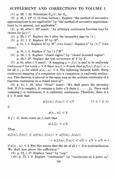
SUPPLEMENT AND CORRECTIONS TO VOLUME 1(1) p. 28, 1. 23. Substitute Ga(X) for Ga.(2) p. 46, 1. 13* (1. 13 from bottom). Replace "the method of successive
approximations is not applicable" by "the method of successive approxima-tions is, in general, not applicable".
(3) p. 49, after 1. 10* insert: "An arbitrary continuous function may bechosen for fo(x) ".
(4) p. 50, 1. 1*. Replace the X after the inequality sign by I X I.
(5) p. 51, 1. 2. Replace M by M2.p. 51, 1. 3. Replace M by (two times). Replace by I (two
times).p. 51, 1. 5. Replace by I
(6) p. 56, 1. 6. Replace "closed region" by "closed bounded region".p. 59, 1. 2*. Replace the first occurrence of V by X.
(7) p. 61, after 1. 9 insert: "A mapping y = f(x) is said to be uniformlycontinuous if for every > 0 there is a 5 > 0 such that p(f(xi),f(x2)) <for all x1, x2 for which p(xi, x2) < & The following theorem holds: Everycontinuous mapping of a compactum into a compactum is uniformly continu-ous. This theorem is proved in the same way as the uniform continuity of afunction continuous on a closed interval".
(8) p. 61, 1. 18. After "Proof" insert: "We shall prove the necessityfirst. If D is compact, D contains a finite fi, ,fN. Since eachmapping is continuous, it is uniformly continuous. Therefore, there is a5 > 0 such that
< (1 i n)
p(x1 , x2) < 5.
If f E D, there exists an such that
Then
p(f(xi),f(x2)) � p(f(xi),f2(xi)) +
+ + + =
if p(xi, x2) < But this means that the set of all f D is equicontinuous.We shall now prove the sufficiency."
(9) p. 72, 1. 3*• Replace "max" by "sup".(10) p. 77, 1. 9. Replace "continuous" by "continuous at a point x0".
123
124 SUPPLEMENT AND CORRECTIONS TO VOL. 1
p. 77, 1. 13. Replace — II by IIx —
p. 77, 1. 11. Replace I f(xi) — f(x2) I byIf(x) — f(xo) I.
p. 77, 1. 20. Replace "continuous" by "uniformly continuous".Delete "everywhere in R".
(11) p. 80, 1. 9*• Replace "x0 L1" by "x0 is a fixed element of thecomplement of Lf".
(12) p. 84, 1. 12. Replace "supn by "5UPn I(13) p. 92, 1. 14*, 13*. The assertion that the functionals generate a
dense subset of C is not true. Replace "satisfies the conditions of Theorem1, i.e. linear combinations of these functionals are everywhere dense inC[a,bl" by "has the property that if a sequence is bounded and
—p for all E then is weakly convergent to x(t)".(14) p. 94, 1. 9* if. The metric introduced here leads to a convergence
which is equivalent to the weak convergence of functionals in every boundedsubset of (but not in all of In 1. 6*, after "so that" insert "in everybounded subset of On p. 95, 1. 10, after "that" insert "for boundedsequences of 1?'.
(15) p. 116. The proof of Theorem 5 contains an error. It should bereplaced by the following:
Proof. 10. We note first that every nonvanishing eigenvalue of a com-pletely continuous operator has finite multiplicity. In fact, the set 14 of alleigenvectors corresponding to an eigenvalue X is a linear subspace whosedimension is equal to the multiplicity of the eigenvalue. If this subspacewere infinite-dimensional for some X 0, the operator A would not becompletely continuous in 14, and hence would not be completely con-tinuous in the whole space.
2°. Now to complete the proof of the theorem it remains to show that ifXnl is a sequence of distinct eigenvalues of a completely continuous op-
erator A, then —p 0 as n —p Let be an eigenvector of A correspond-ing to the eigenvalue The vectors are linearly independent. Let
(n = 1, 2, ...) be the subspace of all the elements of the formn
y
For each y E—1 n n —1 n—i —1y — Ay — j=iajXjXn Xi = i1 (1 — XiXn
whence it is clear that y — Xn1Ay E En_i.Choose a sequence { such that
E En , II yn Ii = 1, p(yn , >
(The existence of such a sequence was proved on p. 118, 1. 6 if.)

SUPPLEMENT AND CORRECTIONS TO VOL. 1 125
We flow suppose that the sequence is bounded. Then the set{A is compact. But this is impossible, since
II— A(yq/Xq)
II
= II — — + A(yq/Xq)] II > (p> q),inasmuch as — + A (yq/Xq) E This contradiction provesthe assertion.
(16) p. 119, 1. 12. The assertion that G0 is a subspace is true, but notobvious. Therefore the sentence "Let G0 be the subspace consisting of allelements of the form x — Ax" should be replaced by the following: "LetG0 be the linear manifold consisting of all elements of the form x — Ax.We shall show that G0 is closed. Let be a one-to-one mapping of thequotient space E/N (where N is the subspace of the elements satisfyingthe condition x — Ax 0) onto G0. (For the definition of quotient spacesee Ex. 5, §57.) We must show that the inverse mapping T' is continuous.It is sufficient to show that it is continuous at y 0. Suppose that this isnot so; then there exists a sequence —p 0 such that p > 0, where
= . Setting fln Sill and = we obtain a sequencesatisfying the conditions:
II fln 11 = 1, 0.
If we choose in each class a representative Xn such that � 2, weobtain a bounded sequence, and = = —
A is completely continuous, contains a fundamental subse-quence The sequence = + (where = andis also fundamental and therefore converges to an element x0. Hence
= —* Tx0, so that Tx0 = 0, that is, x0 E N. But then II I!
— x0 —* 0, which contradicts the condition = 1. This contra-diction proves the continuity of and shows that G0 is closed. Hence G0is a subspace".


Absolutely continuous measure 13abstract Lebesgue measure 32additive measure 20algebra of sets 16almost everywhere (a.e.) 41
B-algebra 19B-measurable function 38B-sets 19Bessel inequality 97bilinear functional 112Boolean ring 20Borel algebra 19Borel closure 19Borel measurable function 38Borel sets 19
INDEX
Cantor function 14characteristic function 42Chebyshev inequality 55closed linear hull 92closed orthonormal set of functions 98closed set of functions 92complete measure 37complete set of functions 92complete set of orthonormal functions 98completely additive measure 11, 28completely continuous operator 115continuous measure 11convergence a.e. 43convergence in measure 44convergence in the mean 84convolution 75countable base for a measure 88
o-algebra 19ô-ring 19direct sum of orthogonal subspaces 108Dirichlet function 48discrete measure 13distribution function 42
Egorov's theorem 43eigenvalues 115eigenvectors 115elementary set 2equivalent functions 41
essentially bounded function 83essential upper bound 83Euclidean space 80extension of a measure 20, 22, 28, 31, 36
Fatou's theorem 59finite partition of a set 17first mean value theorem 55Fourier coefficients 97Fourier series 97fractional integral 76Fubini's theorem 73function integrable over a set 51fundamental in measure 47
Hilbert space 79, 103Holder inequality 83
Infinite-dimensionalspace L2 92inner measure 5, 24, 32inner product 80integral as a set function 77integration by parts 76invariant subset 20isomorphism of 12 and L2 101
Jordan extension of a measure 26, 27Jordan measurable set 23Jordan measure 23
Lebesgue criterion for measurability 15Lebesgue extension of a measure 31, 34Lebesgue integral 48, 51Lebesgue integral of simple functions 48Lebesgue integral as a measure 71Lebesgue measurable set 5, 32Lebesgue measure 8, 32Lebesgue-Stieltjes measures 13Legendre polynomials 93, 96linear functional in Hilbert space 110linear hull 92linear manifold 106linear manifold generated by {cokI 92linearly dependent set of functions 91linearly independent set of functions 91Luzin's theorem 41
127

128 INDEX
Mean convergence 84measurability criterion of Carathéo-
dory 15measurable set 5, 23, 32, 36measure of an elementary set 3measure in Euclidean n-space 12measure 13
measure of a plane set 12measure of a rectangle 2measure on a semi-ring 20minimal B-algebra 19minimal ring 16Minkowski inequality 84,u-integrability for simple functions 49.i-measurable function 38,4F-measurable set 13
n-dimensional space L2 92nonmeasurable sets 13nonseparable Hilbert space 106normalized set of functions 93
Orthogonal complement 107, 110orthogonal set of functions 93orthogonalization process 95orthonormal set of functions 93
Parseval's equality 98, 100plane Lebesgue measure 5product measure 68product of sets 65properties of Lebesgue integral 51ff.
Regular measure 15relation between types of convergence 87Riemann integral 48, 62—64Riesz-Fisher theorem 98ring generated by a collection of sets 16ring of sets 15
function 38scalar product 80Schwarz inequality 105self -adjoint operator 113semi-ring of sets 17set of unicity of a measure 30set of i-unicity 30ti-additive measure 11, 28ti-algebra 19ti-ring 19
simple function 39singular measure 13space 12 79space 79, 80space L9 83space 83space of square integrable functions 79square integrable function 79square summable function 79step function 42subspace 106suhspace generated by 92symmetric bilinear functional 112
Unit of a collection of sets 16Quadratic functional 113quotient space 114 Young's inequality 72


