An m-STAR Model of Dynamic, Endogenous Interdependence – a.k.a. Network-Behavior Coevolution – in the Social Sciences (Prepared for Essex Summer School Wednesday Evening Lecture, 19 August 2009) Jude C. Hays, University of Illinois Aya Kachi, University of Illinois Robert J. Franzese, Jr., University of Michigan
Transcript
An m-STAR Model of Dynamic, Endogenous Interdependence – a.k.a.
Network-Behavior Coevolution – in the Social Sciences
(Prepared for Essex Summer SchoolWednesday Evening Lecture, 19 August 2009)
Jude C. Hays, University of Illinois
Aya Kachi, University of Illinois
Robert J. Franzese, Jr., University of Michigan
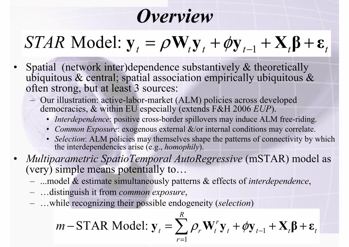
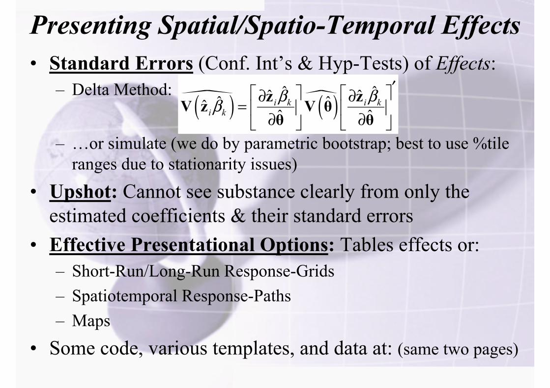
• Spatial (network inter)dependence substantively & theoretically ubiquitous & central; spatial association empirically ubiquitous & often strong, but at least 3 sources:– Our illustration: active-labor-market (ALM) policies across developed
democracies, & within EU especially (extends F&H 2006 EUP).• Interdependence: positive cross-border spillovers may induce ALM free-riding.• Common Exposure: exogenous external &/or internal conditions may correlate.• Selection: ALM policies may themselves shape the patterns of connectivity by which
the interdependencies arise (e.g., homophily).• Multiparametric SpatioTemporal AutoRegressive (mSTAR) model as
(very) simple means potentially to…– ...model & estimate simultaneously patterns & effects of interdependence,– …distinguish it from common exposure,– …while recognizing their possible endogeneity (selection)
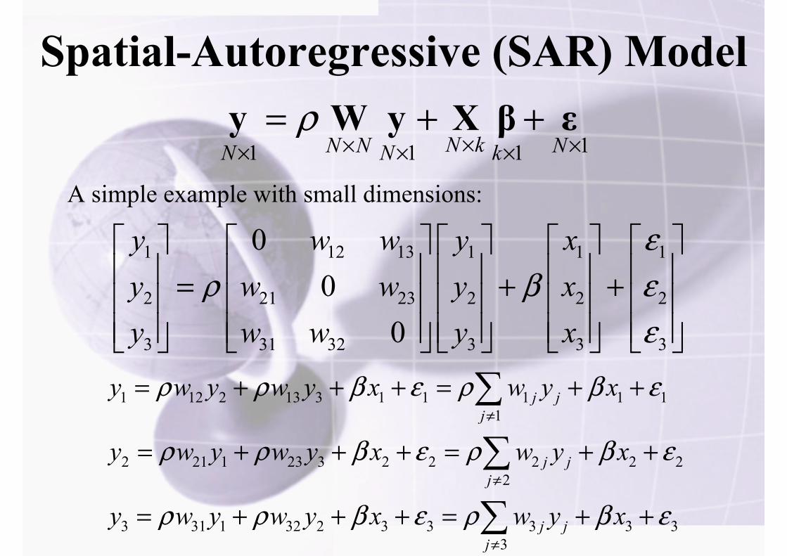
Overview1 Model: t t t t t tSTAR ρ φ −= + + +y W y y X β ε
11
STAR Model: R
rt r t t t t t
rm ρ φ −
=
− = + + +∑y W y y X β ε
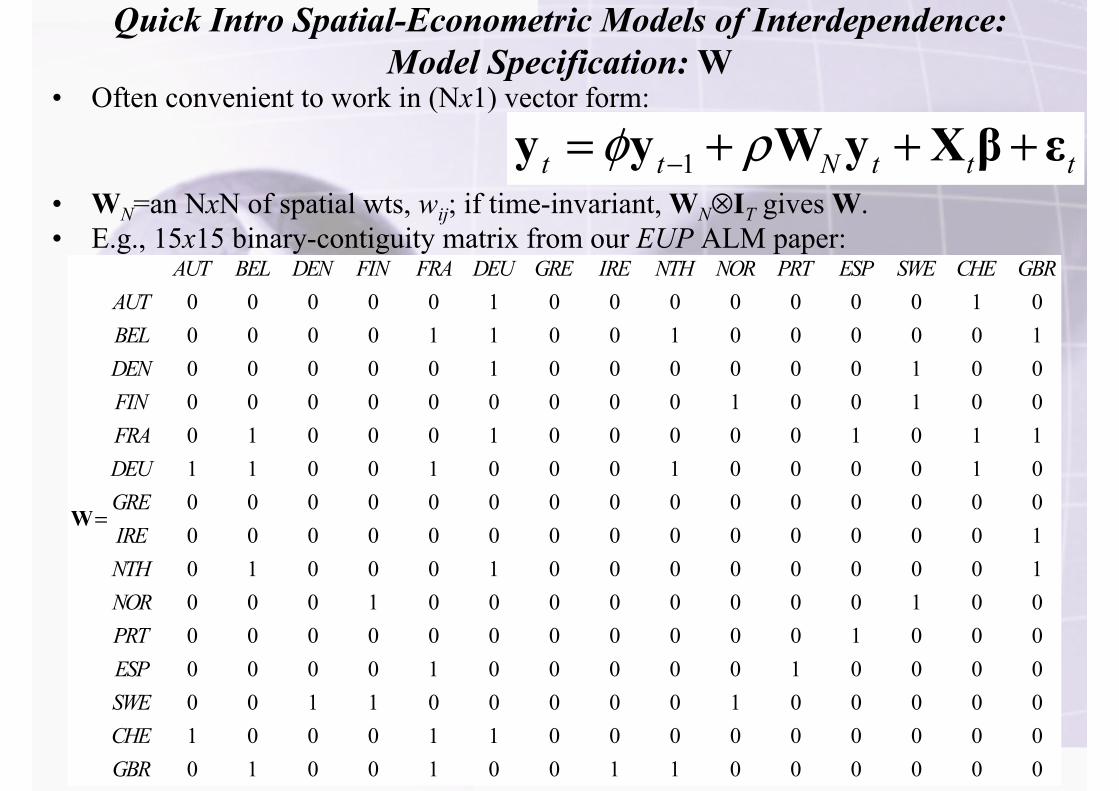
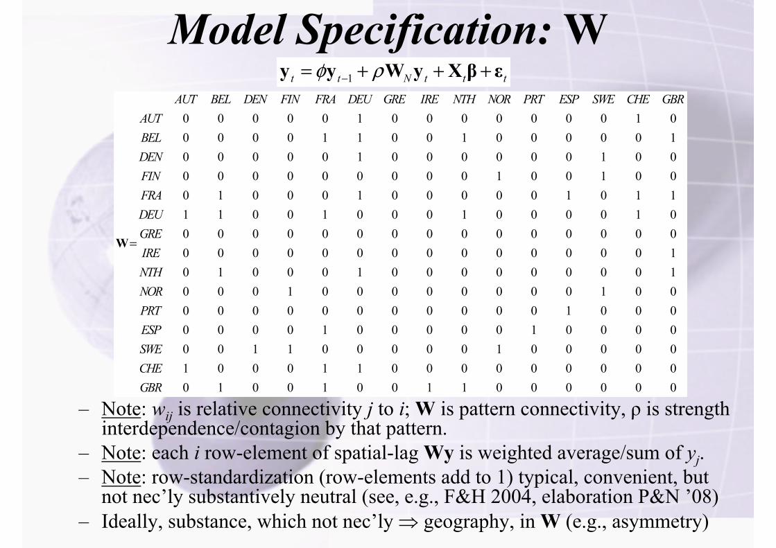
Quick Intro Spatial-Econometric Models of Interdependence:Model Specification: W
• Often convenient to work in (Nx1) vector form:
• WN=an NxN of spatial wts, wij; if time-invariant, WN⊗IT gives W.• E.g., 15x15 binary-contiguity matrix from our EUP ALM paper:
– Note: wij is relative connectivity j to i; W is pattern connectivity, ρ is strength interdependence/contagion by that pattern.
– Note: each i row-element of spatial-lag Wy is weighted average/sum of yj.– Note: row-standardization (row-elements add to 1) typical, convenient, but
not nec’ly substantively neutral (see, e.g., F&H 2004, elaboration P&N ’08)– Ideally, substance, which not nec’ly ⇒ geography, in W (e.g., asymmetry)
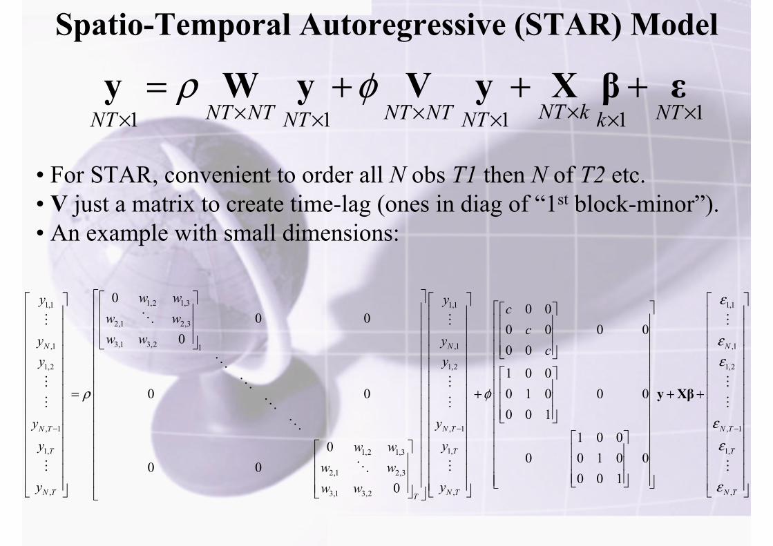
• For STAR, convenient to order all N obs T1 then N of T2 etc.• V just a matrix to create time-lag (ones in diag of “1st block-minor”).• An example with small dimensions:
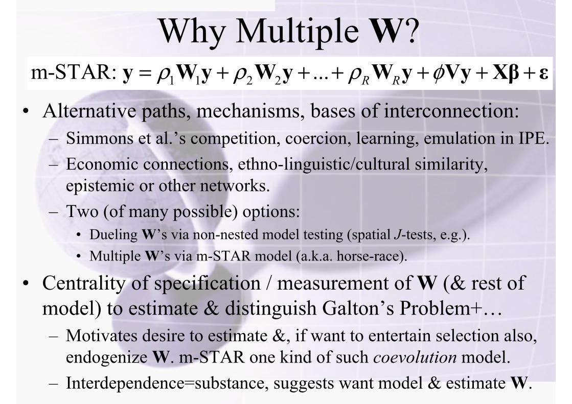
Why Multiple W?
• Alternative paths, mechanisms, bases of interconnection:– Simmons et al.’s competition, coercion, learning, emulation in IPE.– Economic connections, ethno-linguistic/cultural similarity,
epistemic or other networks.– Two (of many possible) options:
• Dueling W’s via non-nested model testing (spatial J-tests, e.g.).• Multiple W’s via m-STAR model (a.k.a. horse-race).
• Centrality of specification / measurement of W (& rest of model) to estimate & distinguish Galton’s Problem+…– Motivates desire to estimate &, if want to entertain selection also,
endogenize W. m-STAR one kind of such coevolution model.– Interdependence=substance, suggests want model & estimate W.
1 1 2 2m-STAR: ... R Rρ ρ ρ φ= + + + + + +y W y W y W y Vy Xβ ε
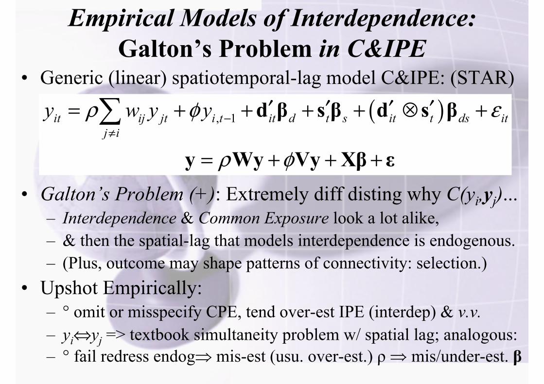
Empirical Models of Interdependence:Galton’s Problem in C&IPE
• Generic (linear) spatiotemporal-lag model C&IPE: (STAR)
• Galton’s Problem (+): Extremely diff disting why C(yi,yj)...– Interdependence & Common Exposure look a lot alike,– & then the spatial-lag that models interdependence is endogenous.– (Plus, outcome may shape patterns of connectivity: selection.)
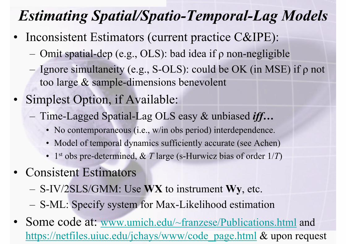
• No contemporaneous (i.e., w/in obs period) interdependence.• Model of temporal dynamics sufficiently accurate (see Achen)• 1st obs pre-determined, & T large (s-Hurwicz bias of order 1/T)
• Consistent Estimators– S-IV/2SLS/GMM: Use WX to instrument Wy, etc.– S-ML: Specify system for Max-Likelihood estimation
• Some code at: www.umich.edu/~franzese/Publications.html and https://netfiles.uiuc.edu/jchays/www/code_page.html & upon request
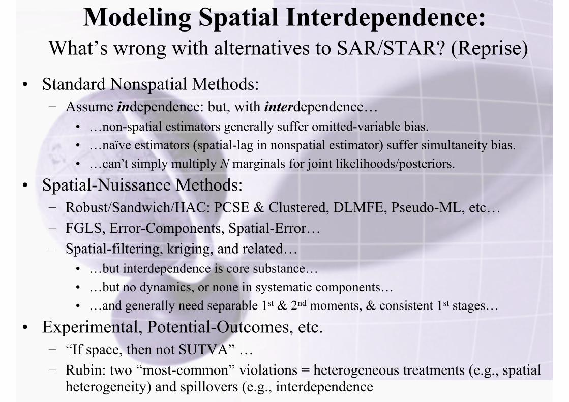
• Standard Nonspatial Methods:– Assume independence: but, with interdependence…
• …non-spatial estimators generally suffer omitted-variable bias.• …naïve estimators (spatial-lag in nonspatial estimator) suffer simultaneity bias.• …can’t simply multiply N marginals for joint likelihoods/posteriors.
• …but interdependence is core substance…• …but no dynamics, or none in systematic components…• …and generally need separable 1st & 2nd moments, & consistent 1st stages…
• Experimental, Potential-Outcomes, etc.– “If space, then not SUTVA” …– Rubin: two “most-common” violations = heterogeneous treatments (e.g., spatial
heterogeneity) and spillovers (e.g., interdependence
Modeling Spatial Interdependence:What’s wrong with alternatives to SAR/STAR? (Reprise)
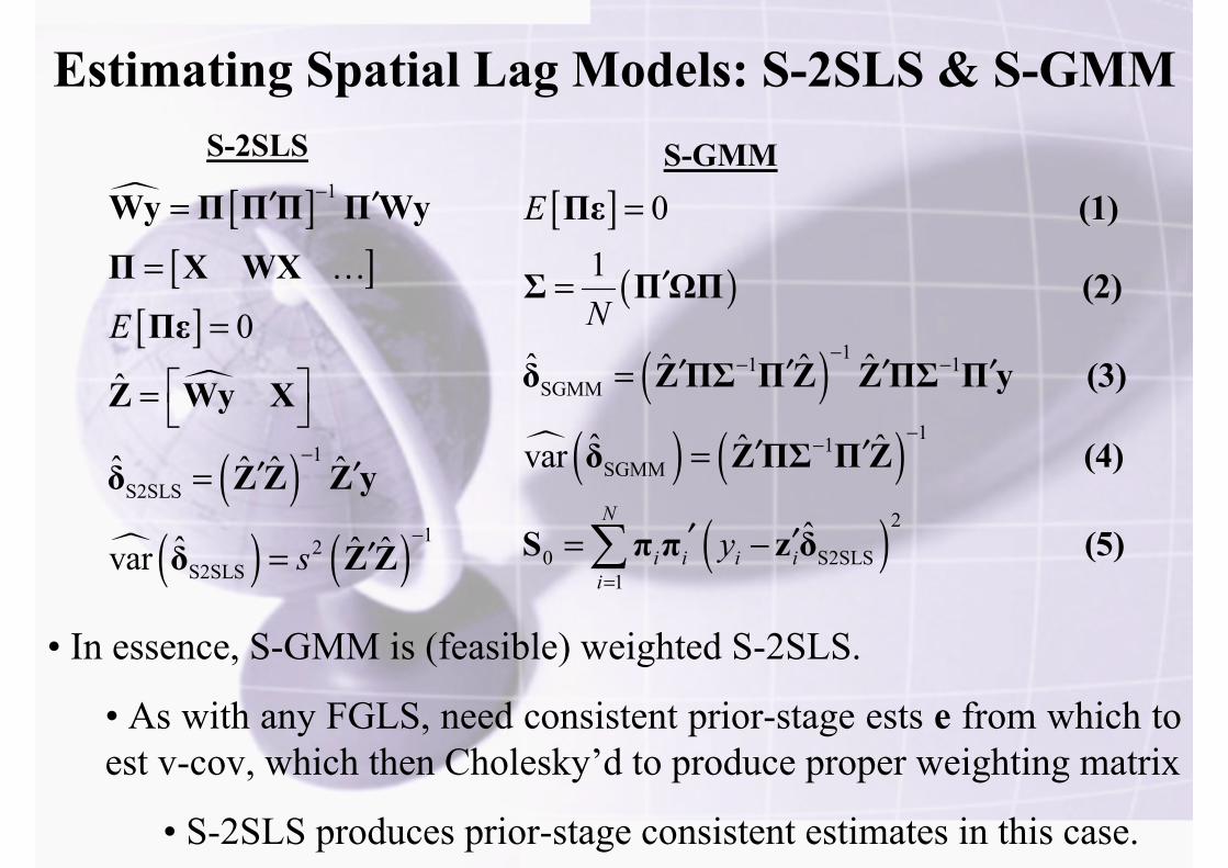
Estimating Spatial Lag Models: S-2SLS & S-GMM
[ ][ ]
[ ]
( )( ) ( )
1
1
S2SLS
12S2SLS
0
ˆ
ˆ ˆ ˆ ˆ
ˆ ˆ ˆvar
E
s
−
−
−
′ ′=
=
=
⎡ ⎤= ⎣ ⎦
′ ′=
′=
Wy Π ΠΠ Π Wy
Π X WX
Πε
Z Wy X
δ Z Z Z y
δ Z Z
…[ ]
( )
( )( ) ( )
11 1SGMM
11SGMM
01
0 1
ˆ ˆ ˆ ˆ
ˆ ˆ ˆvar N
ii
E
N−− −
−−
=
=
′=
′ ′ ′ ′=
′ ′=
=∑
Πε (1)
Σ ΠΩΠ (2)
δ Z ΠΣ Π Z Z ΠΣ Π y (3)
δ Z ΠΣ Π Z (4)
S π π ( )2
S2SLSˆ i i iy′ ′− z δ (5)
• In essence, S-GMM is (feasible) weighted S-2SLS.
• As with any FGLS, need consistent prior-stage ests e from which to est v-cov, which then Cholesky’d to produce proper weighting matrix
• S-2SLS produces prior-stage consistent estimates in this case.
S-2SLS S-GMM
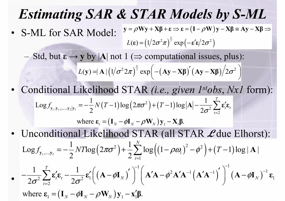
Estimating SAR & STAR Models by S-ML• S-ML for SAR Model:
– Std, but ε→ y by |A| not 1 (⇒ computational issues, plus):
• Conditional Likelihood STAR (i.e., given 1stobs, Nx1 form):
• Unconditional Likelihood STAR (all STAR L due Elhorst):
•
( )
( ) ( )22 2( ) 1 2 exp 2N
L
ρ ρ
σ π σ
= + + ⇒ = − − ≡ − ⇒
′= −
y Wy Xβ ε ε I W y Xβ Ay Xβ
ε ε ε
( ) ( ) ( )22 2( ) | | 1 2 exp 2N
L σ π σ⎛ ⎞′= − − −⎜ ⎟⎝ ⎠
y A Ay Xβ Ay Xβ
( ) ( ) ( )
( )1 2 1
2, ,..., 2
2
1 1Log 1 log 2 1 log2 2
where .
t t
T
t tt
t N N N t t
f N T Tπσσ
φ ρ
−=
′= − − + − −
= − − −
∑y y y y A ε ε
ε I I W y X β
( ) ( )( ) ( )
( ) ( ) ( )
( )
1
22 2,...,
111
12 1 11 12 2
2
1 1 1
1 1Log log 2 log 1 1 log | |2 2
1 12 2
where .
t
N
ii
T
t t N Nt
N N N
f NT Tπσ ρω φ
φ φ φσ σ
φ ρ
=
−−−− −
=
= − + − − + −
⎛ ⎞′⎛ ⎞′′ ′ ′ ′ ′− − − − −⎜ ⎟ ⎜ ⎟⎝ ⎠ ⎝ ⎠′= − − −
∑
∑
y y A
ε ε ε A I A A A A A A A I ε
ε I I W y x β
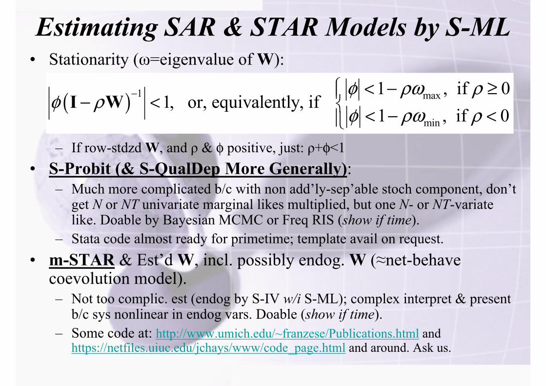
Estimating SAR & STAR Models by S-ML• Stationarity (ω=eigenvalue of W):
– If row-stdzd W, and ρ & φ positive, just: ρ+φ<1• S-Probit (& S-QualDep More Generally):
– Much more complicated b/c with non add’ly-sep’able stoch component, don’t get N or NT univariate marginal likes multiplied, but one N- or NT-variatelike. Doable by Bayesian MCMC or Freq RIS (show if time).
– Stata code almost ready for primetime; template avail on request.• m-STAR & Est’d W, incl. possibly endog. W (≈net-behave
coevolution model).– Not too complic. est (endog by S-IV w/i S-ML); complex interpret & present
b/c sys nonlinear in endog vars. Doable (show if time).– Some code at: http://www.umich.edu/~franzese/Publications.html and
https://netfiles.uiuc.edu/jchays/www/code_page.html and around. Ask us.
( ) 1 max
min
1 , if 01, or, equivalently, if
1 , if 0φ ρω ρ
φ ρφ ρω ρ
− ⎧ < − ≥⎪− < ⎨ < − <⎪⎩I W
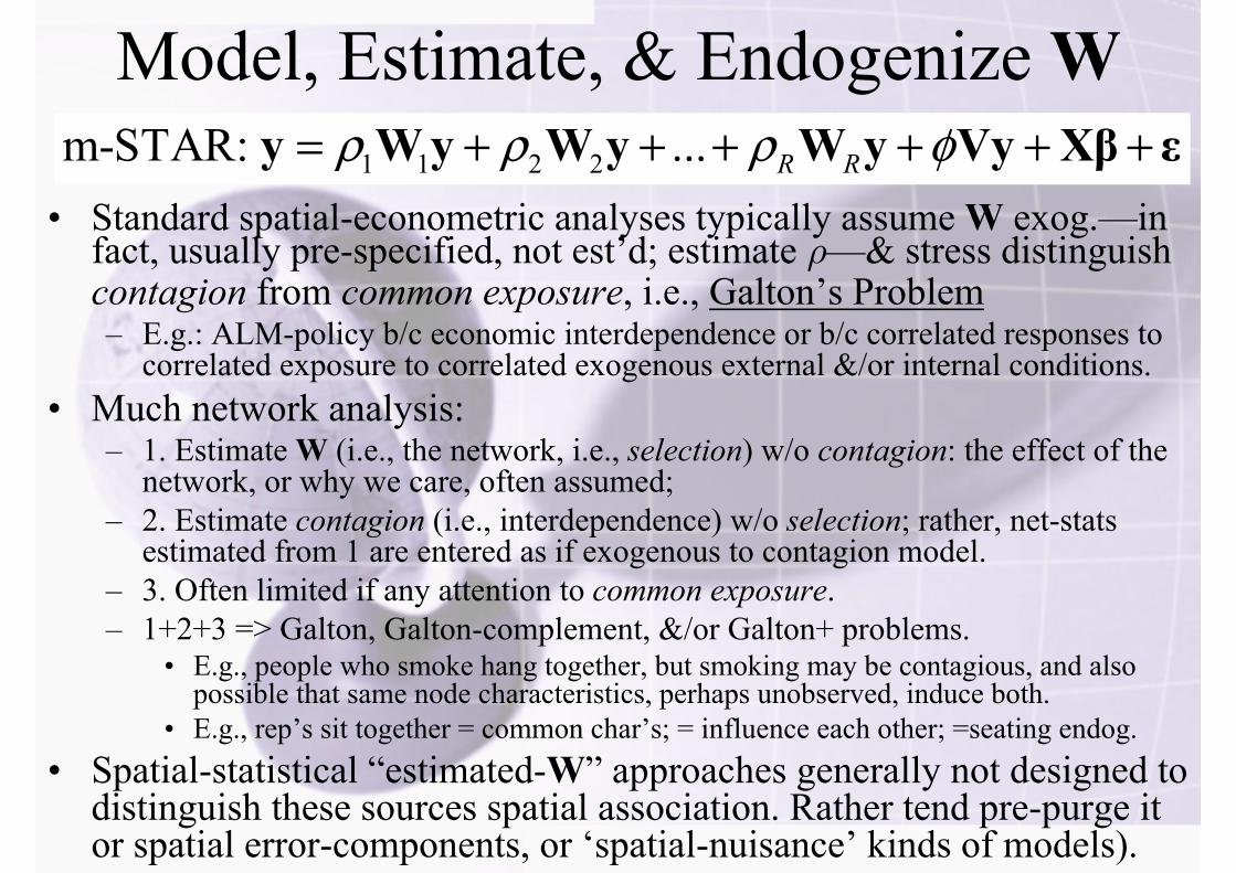
Model, Estimate, & Endogenize W
• Standard spatial-econometric analyses typically assume W exog.—in fact, usually pre-specified, not est’d; estimate ρ—& stress distinguish contagion from common exposure, i.e., Galton’s Problem– E.g.: ALM-policy b/c economic interdependence or b/c correlated responses to
correlated exposure to correlated exogenous external &/or internal conditions.• Much network analysis:
– 1. Estimate W (i.e., the network, i.e., selection) w/o contagion: the effect of the network, or why we care, often assumed;
– 2. Estimate contagion (i.e., interdependence) w/o selection; rather, net-stats estimated from 1 are entered as if exogenous to contagion model.
– 3. Often limited if any attention to common exposure.– 1+2+3 => Galton, Galton-complement, &/or Galton+ problems.
• E.g., people who smoke hang together, but smoking may be contagious, and also possible that same node characteristics, perhaps unobserved, induce both.
• E.g., rep’s sit together = common char’s; = influence each other; =seating endog.• Spatial-statistical “estimated-W” approaches generally not designed to
distinguish these sources spatial association. Rather tend pre-purge it or spatial error-components, or ‘spatial-nuisance’ kinds of models).
1 1 2 2m-STAR: ... R Rρ ρ ρ φ= + + + + + +y W y W y W y Vy Xβ ε
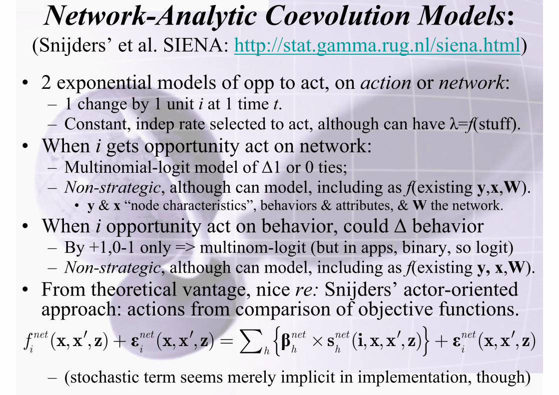
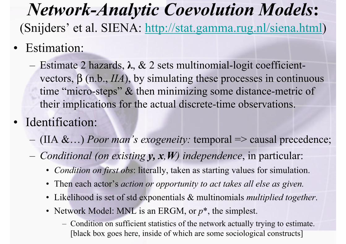
Network-Analytic Coevolution Models:(Snijders’ et al. SIENA: http://stat.gamma.rug.nl/siena.html)
• 2 exponential models of opp to act, on action or network:– 1 change by 1 unit i at 1 time t.– Constant, indep rate selected to act, although can have λ=f(stuff).
• When i gets opportunity act on network:– Multinomial-logit model of Δ1 or 0 ties;– Non-strategic, although can model, including as f(existing y,x,W).
• y & x “node characteristics”, behaviors & attributes, & W the network.• When i opportunity act on behavior, could Δ behavior
– By +1,0-1 only => multinom-logit (but in apps, binary, so logit)– Non-strategic, although can model, including as f(existing y, x,W).
• From theoretical vantage, nice re: Snijders’ actor-oriented approach: actions from comparison of objective functions.
– (stochastic term seems merely implicit in implementation, though)
( , , ) ( , , ) ( , , , ) ( , , )net net net net neti i h h ihf ′ ′ ′ ′+ = × +∑x x z x x z s i x x z x x zε β ε
Network-Analytic Coevolution Models:(Snijders’ et al. SIENA: http://stat.gamma.rug.nl/siena.html)
vectors, β (n.b., IIA), by simulating these processes in continuous time “micro-steps” & then minimizing some distance-metric of their implications for the actual discrete-time observations.
• Identification:– (IIA &…) Poor man’s exogeneity: temporal => causal precedence;– Conditional (on existing y, x,W) independence, in particular:
• Condition on first obs: literally, taken as starting values for simulation.• Then each actor’s action or opportunity to act takes all else as given.• Likelihood is set of std exponentials & multinomials multiplied together.• Network Model: MNL is an ERGM, or p*, the simplest.
– Condition on sufficient statistics of the network actually trying to estimate. [black box goes here, inside of which are some sociological constructs]
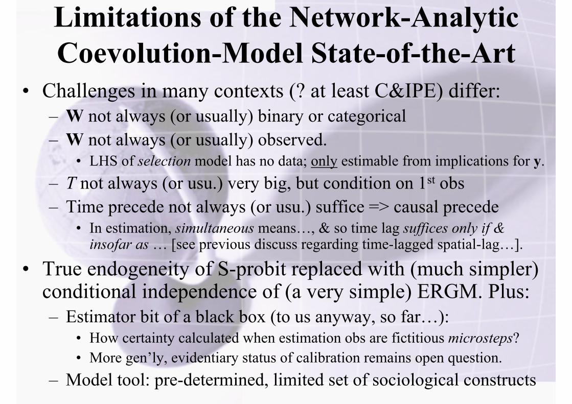
Limitations of the Network-Analytic Coevolution-Model State-of-the-Art
• Challenges in many contexts (? at least C&IPE) differ:– W not always (or usually) binary or categorical– W not always (or usually) observed.
• LHS of selection model has no data; only estimable from implications for y.– T not always (or usu.) very big, but condition on 1st obs– Time precede not always (or usu.) suffice => causal precede
• In estimation, simultaneous means…, & so time lag suffices only if & insofar as … [see previous discuss regarding time-lagged spatial-lag…].
• True endogeneity of S-probit replaced with (much simpler) conditional independence of (a very simple) ERGM. Plus:– Estimator bit of a black box (to us anyway, so far…):
• How certainty calculated when estimation obs are fictitious microsteps?• More gen’ly, evidentiary status of calibration remains open question.
– Model tool: pre-determined, limited set of sociological constructs
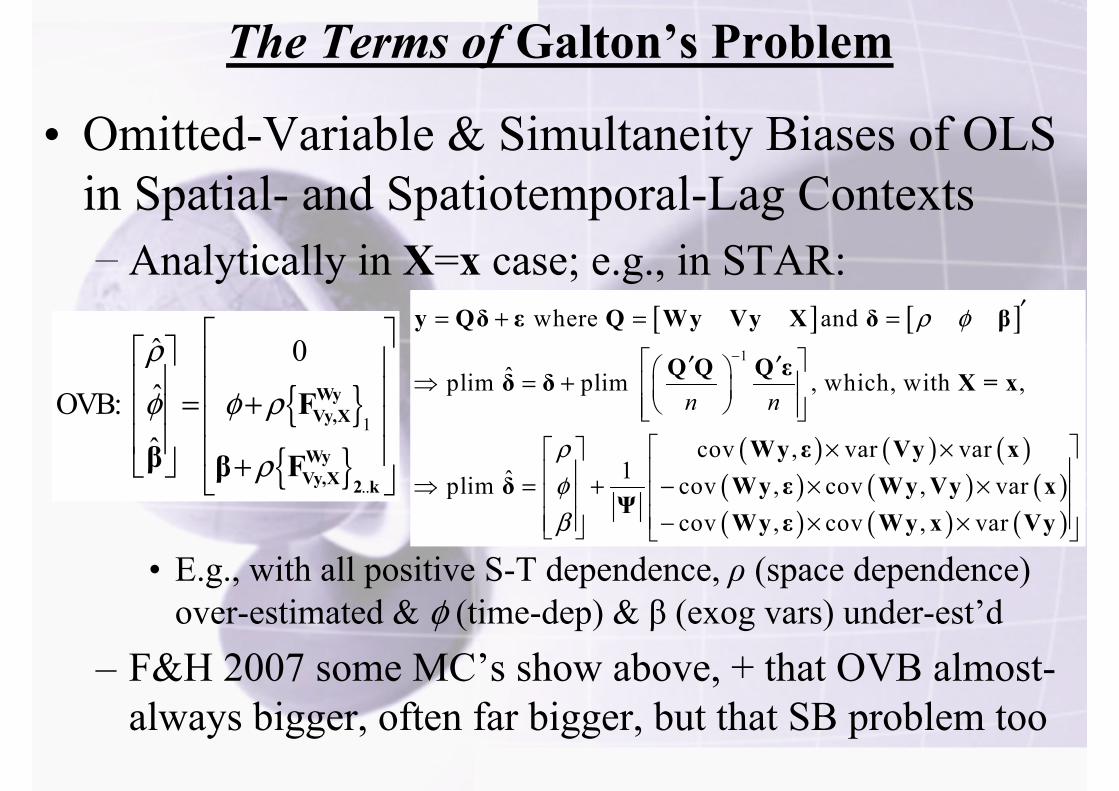
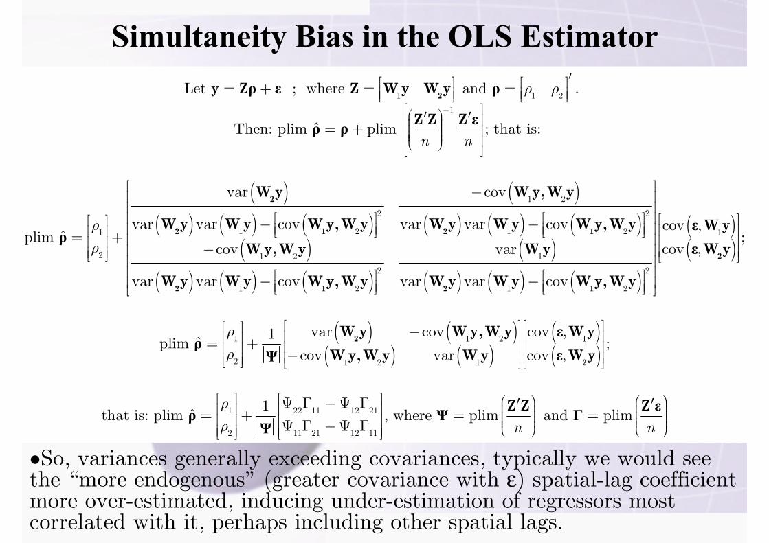
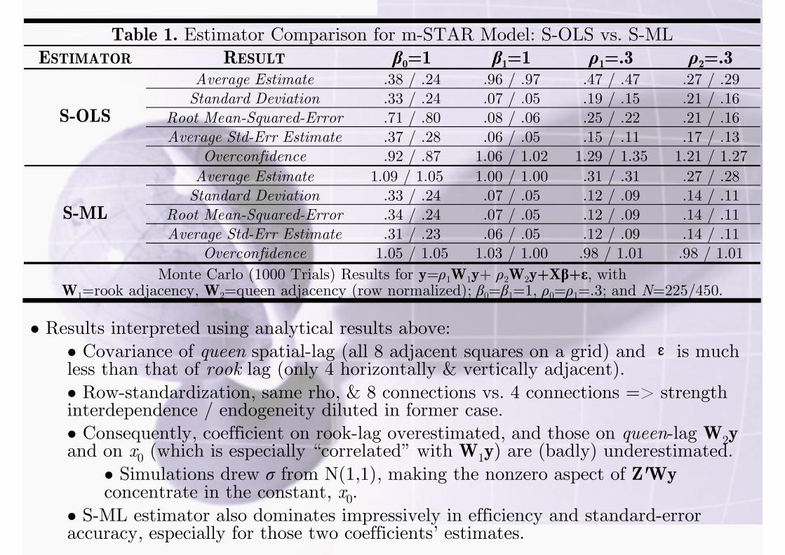
•So, variances generally exceeding covariances, typically we would see the “more endogenous” (greater covariance with ε) spatial-lag coefficient more over-estimated, inducing under-estimation of regressors most correlated with it, perhaps including other spatial lags.
Table 1. Estimator Comparison for m-STAR Model: S-OLS vs. S-ML ESTIMATOR RESULT β0=1 β1=1 ρ1=.3 ρ2=.3
Overconfidence 1.05 / 1.05 1.03 / 1.00 .98 / 1.01 .98 / 1.01 Monte Carlo (1000 Trials) Results for y=ρ1W1y+ ρ2W2y+Xβ+ε, with
W1=rook adjacency, W2=queen adjacency (row normalized); β0=β1=1, ρ0=ρ1=.3; and N=225/450.
• Results interpreted using analytical results above:
• Covariance of queen spatial-lag (all 8 adjacent squares on a grid) and ε is much less than that of rook lag (only 4 horizontally & vertically adjacent).• Row-standardization, same rho, & 8 connections vs. 4 connections => strength interdependence / endogeneity diluted in former case.• Consequently, coefficient on rook-lag overestimated, and those on queen-lag W2yand on x0 (which is especially “correlated” with W1y) are (badly) underestimated.
• Simulations drew σ from N(1,1), making the nonzero aspect of Z'Wyconcentrate in the constant, x0.
• S-ML estimator also dominates impressively in efficiency and standard-error accuracy, especially for those two coefficients’ estimates.
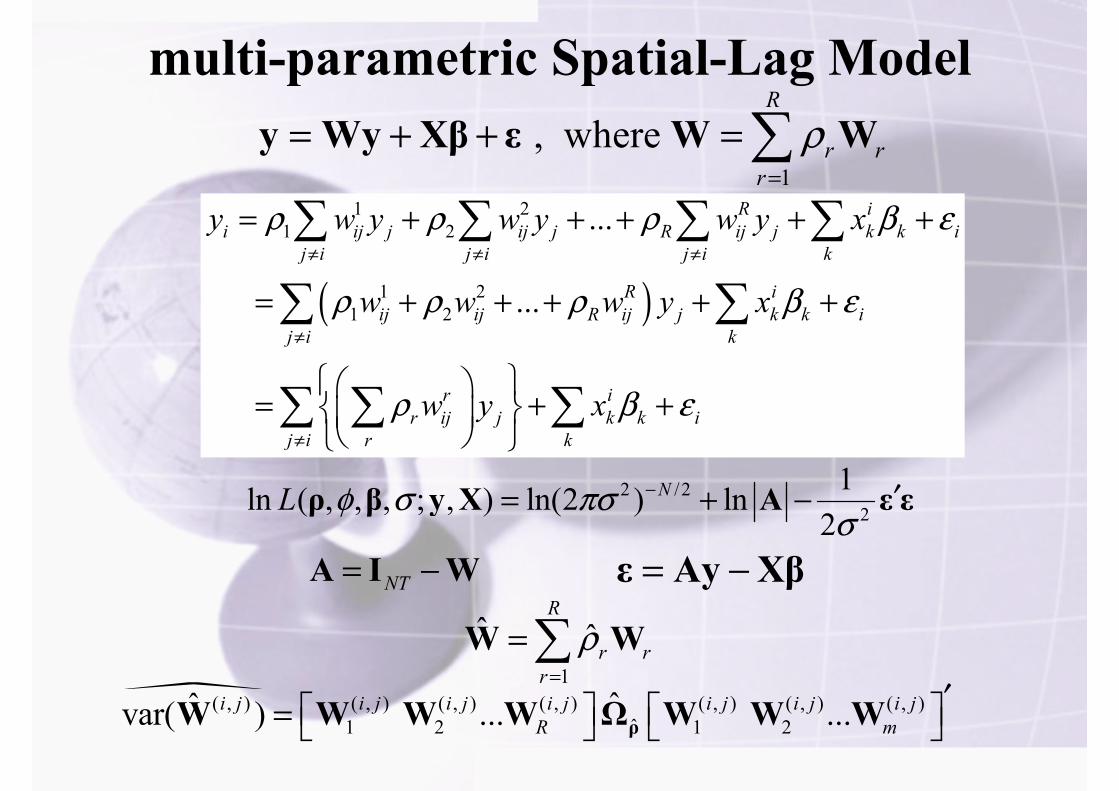
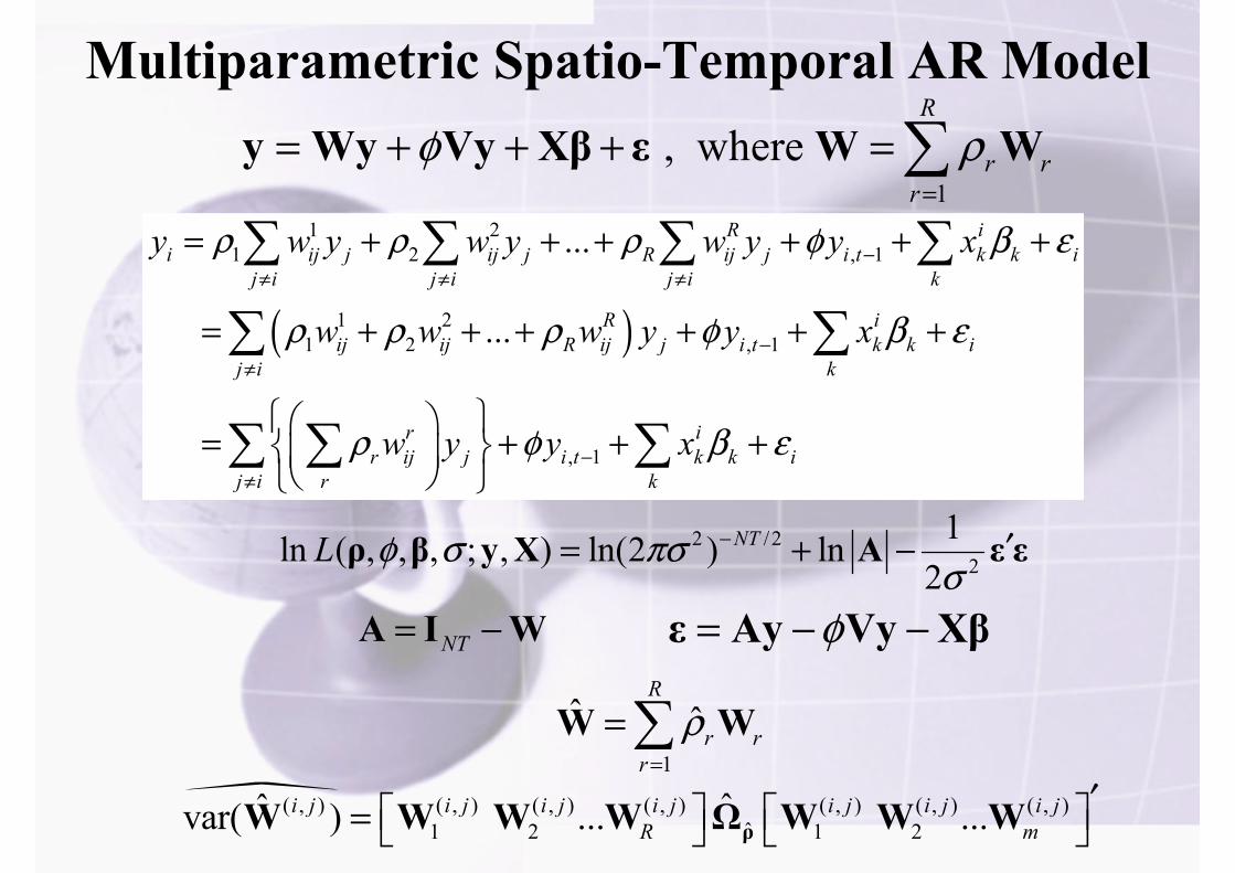
Multiparametric Spatio-Temporal AR Model
1 , where
R
r rr
φ ρ=
= + + + =∑y Wy Vy Xβ ε W W
( , ) ( , ) ( , ) ( , ) ( , ) ( , ) ( , )ˆ1 2 1 2
ˆˆvar( ) ... ...i j i j i j i j i j i j i jR m
′⎡ ⎤ ⎡ ⎤= ⎣ ⎦ ⎣ ⎦ρW W W W Ω W W W
2 /22
1ln ( , , , ; , ) ln(2 ) ln2
NTL φ σ πσσ
− ′= + −ρ β y X A ε ε
NT= −A I W φ= − −ε Ay Vy Xβ
1
ˆ ˆR
r rr
ρ=
=∑W W
( )
1 21 2 , 1
1 21 2 , 1
, 1
...
...
R ii ij j ij j R ij j i t k k i
j i j i j i k
R iij ij R ij j i t k k i
j i k
r ir ij j i t k k i
j i r k
y w y w y w y y x
w w w y y x
w y y x
ρ ρ ρ φ β ε
ρ ρ ρ φ β ε
ρ φ β ε
−≠ ≠ ≠
−≠
−≠
= + + + + + +
= + + + + + +
⎧ ⎫⎛ ⎞= + + +⎨ ⎬⎜ ⎟⎝ ⎠⎩ ⎭
∑ ∑ ∑ ∑
∑ ∑
∑ ∑ ∑
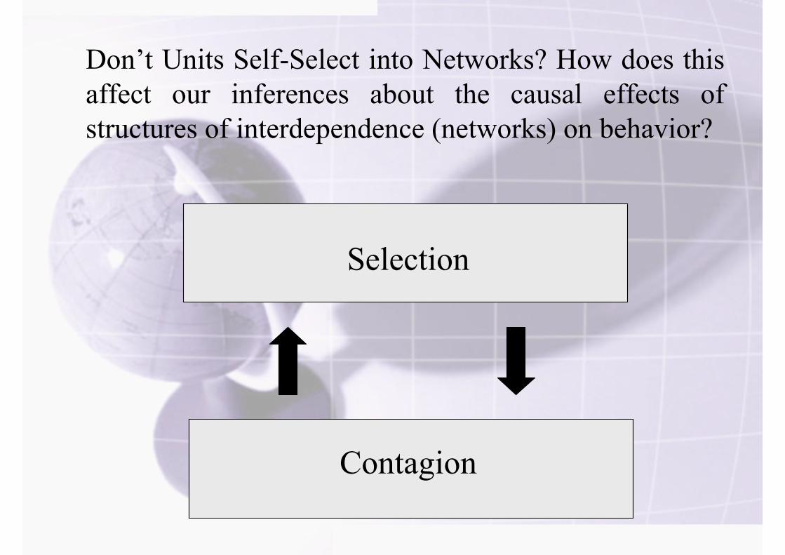
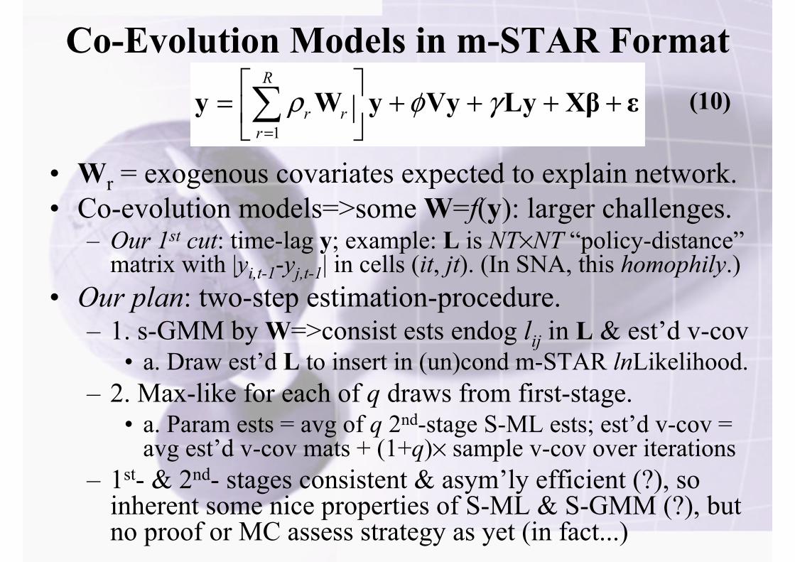
Don’t Units Self-Select into Networks? How does this affect our inferences about the causal effects of structures of interdependence (networks) on behavior?
– Our 1st cut: time-lag y; example: L is NT%NT “policy-distance”matrix with |yi,t-1-yj,t-1| in cells (it, jt). (In SNA, this homophily.)
• Our plan: two-step estimation-procedure.– 1. s-GMM by W=>consist ests endog lij in L & est’d v-cov
• a. Draw est’d L to insert in (un)cond m-STAR lnLikelihood.– 2. Max-like for each of q draws from first-stage.
• a. Param ests = avg of q 2nd-stage S-ML ests; est’d v-cov = avg est’d v-cov mats + (1+q)% sample v-cov over iterations
– 1st- & 2nd- stages consistent & asym’ly efficient (?), so inherent some nice properties of S-ML & S-GMM (?), but no proof or MC assess strategy as yet (in fact...)
1
R
r rr
ρ φ γ=
⎡ ⎤= + + + +⎢ ⎥⎣ ⎦∑y W y Vy Ly Xβ ε (10)
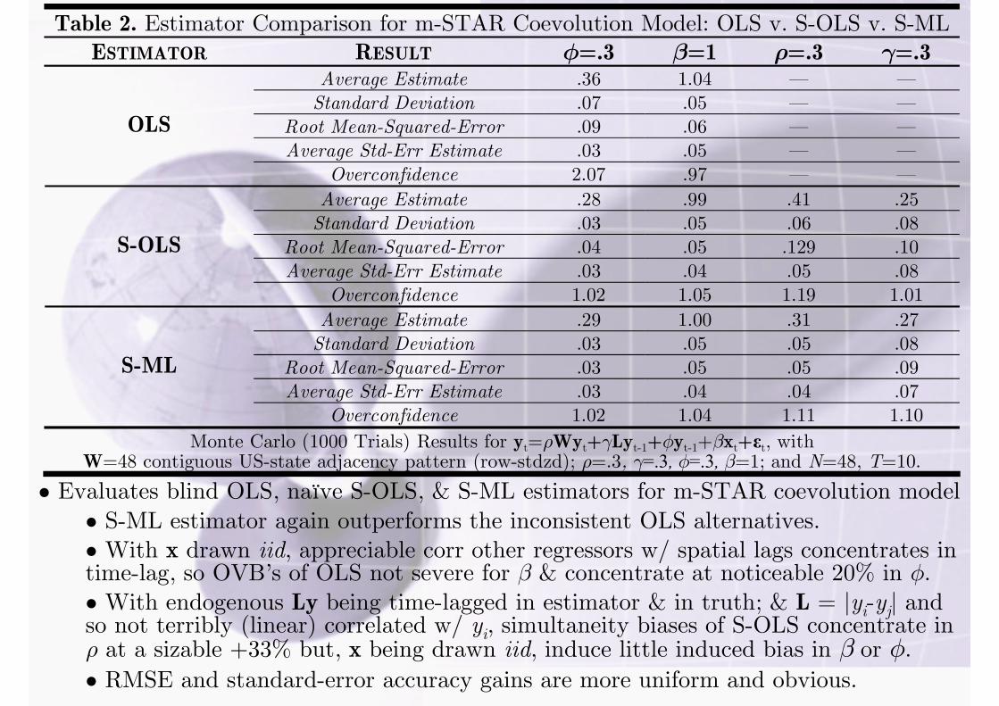
• Evaluates blind OLS, naïve S-OLS, & S-ML estimators for m-STAR coevolution model• S-ML estimator again outperforms the inconsistent OLS alternatives.• With x drawn iid, appreciable corr other regressors w/ spatial lags concentrates in time-lag, so OVB’s of OLS not severe for β & concentrate at noticeable 20% in φ.• With endogenous Ly being time-lagged in estimator & in truth; & L = |yi-yj| and so not terribly (linear) correlated w/ yi, simultaneity biases of S-OLS concentrate in ρ at a sizable +33% but, x being drawn iid, induce little induced bias in β or φ.• RMSE and standard-error accuracy gains are more uniform and obvious.
Table 2. Estimator Comparison for m-STAR Coevolution Model: OLS v. S-OLS v. S-ML ESTIMATOR RESULT φ=.3 β=1 ρ=.3 γ=.3
Average Estimate .36 1.04 — — Standard Deviation .07 .05 — —
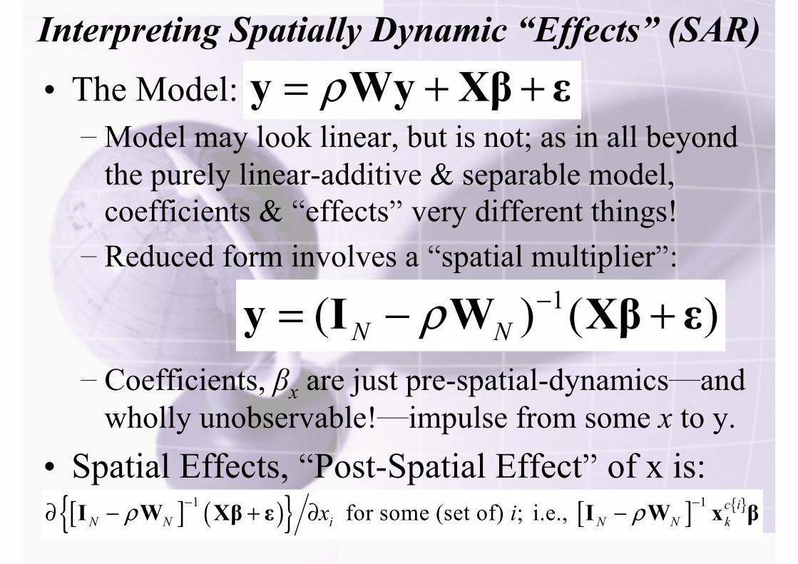
Interpreting Spatially Dynamic “Effects” (SAR)• The Model:–Model may look linear, but is not; as in all beyond
the purely linear-additive & separable model, coefficients & “effects” very different things!– Reduced form involves a “spatial multiplier”:
– Coefficients, βx are just pre-spatial-dynamics—and wholly unobservable!—impulse from some x to y.
• Spatial Effects, “Post-Spatial Effect” of x is:
ρ= + +y Wy Xβ ε
1( ) ( )N Nρ −= − +y I W Xβ ε
[ ] ( ) [ ] 1 1 for some (set of) ; i.e., c iN N i N N kx iρ ρ− −∂ − + ∂ −I W Xβ ε I W x β
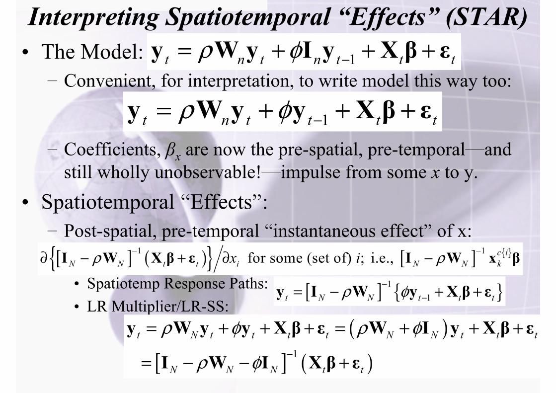
Interpreting Spatiotemporal “Effects” (STAR)• The Model:– Convenient, for interpretation, to write model this way too:
– Coefficients, βx are now the pre-spatial, pre-temporal—and still wholly unobservable!—impulse from some x to y.
• Spatiotemporal “Effects”:– Post-spatial, pre-temporal “instantaneous effect” of x:
• Spatiotemp Response Paths:• LR Multiplier/LR-SS:
1t n t n t t tρ φ −= + + +y W y I y X β ε
1t n t t t tρ φ −= + + +y W y y X β ε
[ ] 11t N N t t tρ φ−
−= − + +y I W y X β ε
[ ] ( ) [ ] 1 1 for some (set of) ; i.e., c iN N t t i N N kx iρ ρ− −∂ − + ∂ −I W X β ε I W x β
( )[ ] ( )1
ρ φ ρ φ
ρ φ −
= + + + = + + +
= − − +
t N t t t t N N t t t
N N N t t
y W y y X β ε W I y X β ε
I W I X β ε
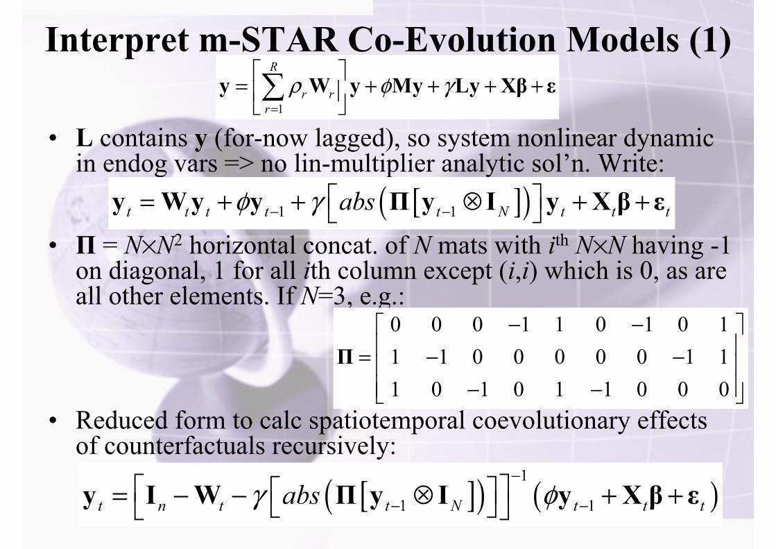
Interpret m-STAR Co-Evolution Models (1)
• L contains y (for-now lagged), so system nonlinear dynamic in endog vars => no lin-multiplier analytic sol’n. Write:
• Π = N%N2 horizontal concat. of N mats with ith N%N having -1 on diagonal, 1 for all ith column except (i,i) which is 0, as are all other elements. If N=3, e.g.:
• Reduced form to calc spatiotemporal coevolutionary effects of counterfactuals recursively:
1
R
r rr
ρ φ γ=
⎡ ⎤= + + + +⎢ ⎥⎣ ⎦∑y W y My Ly Xβ ε
[ ]( )1 1t t t t t N t t tabsφ γ− −⎡ ⎤= + + ⊗ + +⎣ ⎦y W y y Π y I y X β ε
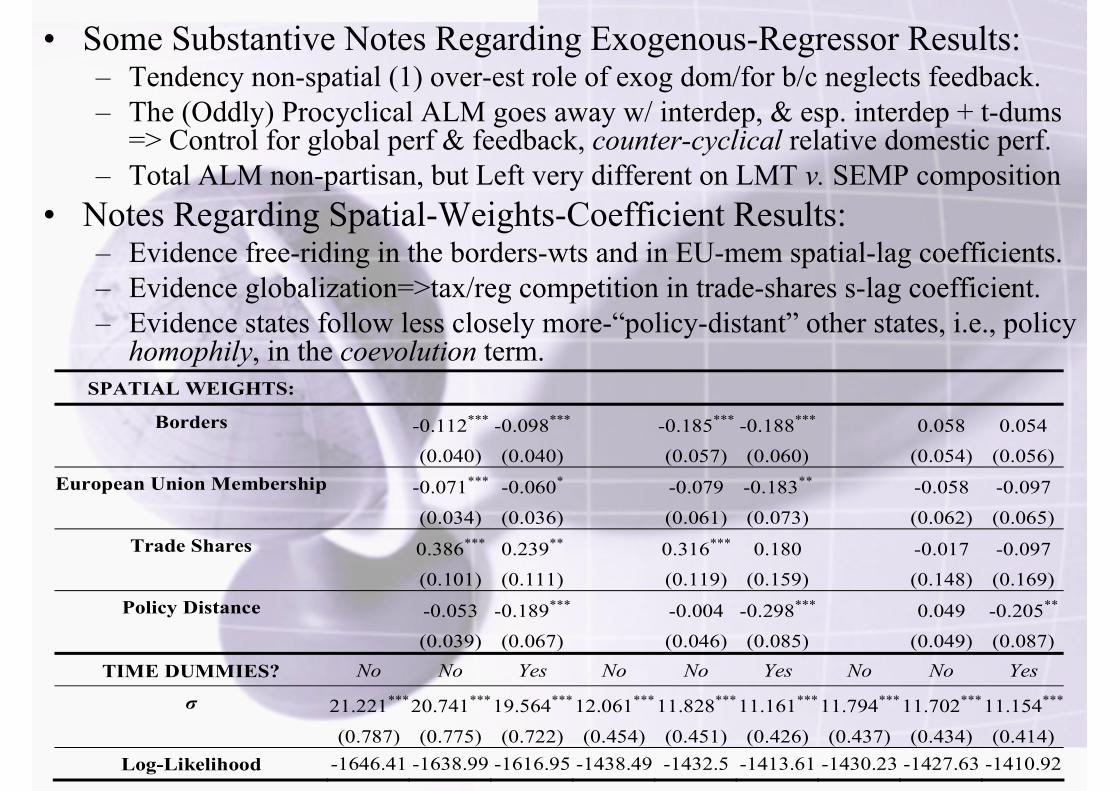
• Some Substantive Notes Regarding Exogenous-Regressor Results:– Tendency non-spatial (1) over-est role of exog dom/for b/c neglects feedback.– The (Oddly) Procyclical ALM goes away w/ interdep, & esp. interdep + t-dums
=> Control for global perf & feedback, counter-cyclical relative domestic perf.– Total ALM non-partisan, but Left very different on LMT v. SEMP composition
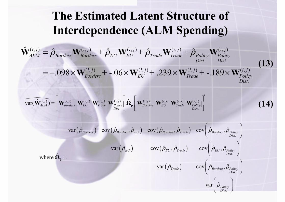
• Notes Regarding Spatial-Weights-Coefficient Results:– Evidence free-riding in the borders-wts and in EU-mem spatial-lag coefficients.– Evidence globalization=>tax/reg competition in trade-shares s-lag coefficient.– Evidence states follow less closely more-“policy-distant” other states, i.e., policy
homophily, in the coevolution term.
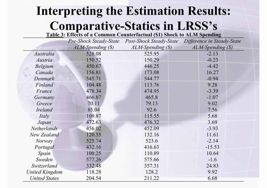
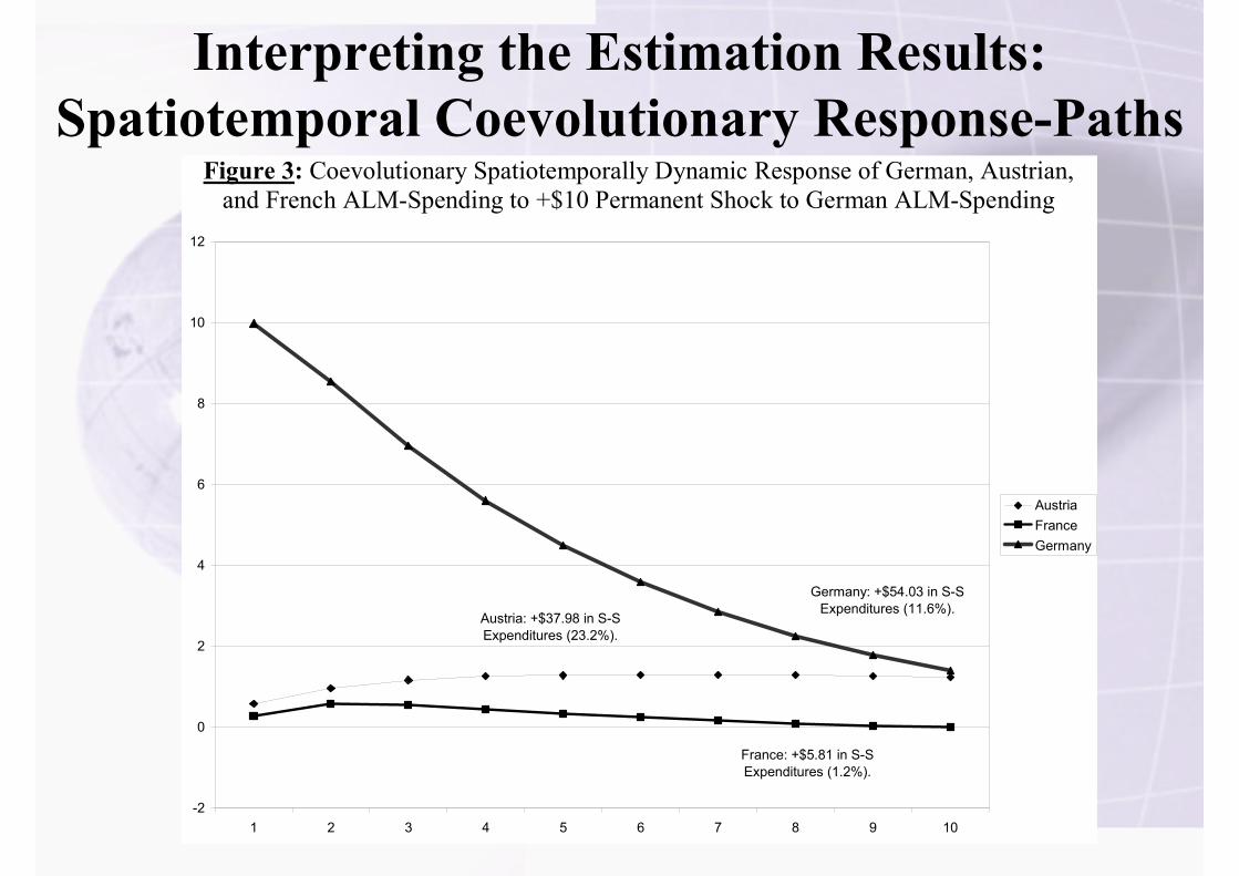
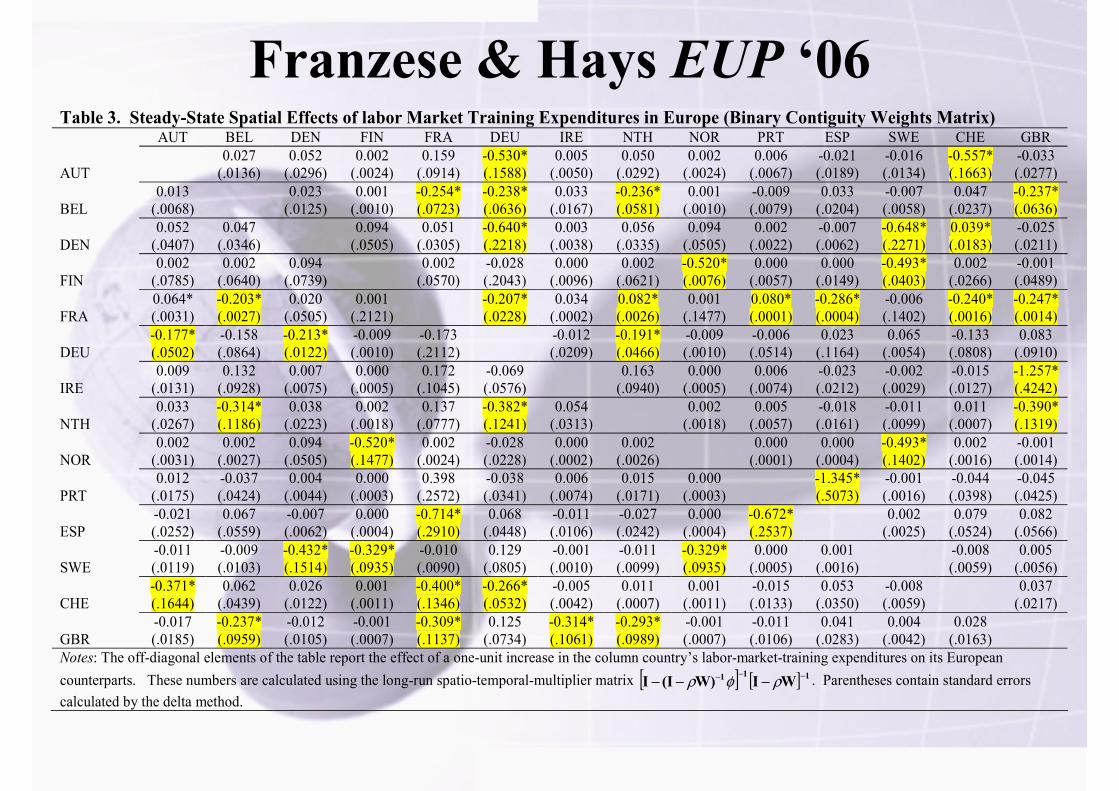
Table 3: Effects of a Common Counterfactual ($1) Shock to ALM Spending
Pre-Shock Steady-State ALM-Spending ($)
Post-Shock Steady-State ALM-Spending ($)
Difference in Steady-State ALM-Spending ($)
Australia 528.08 525.95 -2.13 Austria 150.52 150.29 -0.23 Belgium 450.67 446.25 -4.42 Canada 156.81 173.08 16.27
Denmark 545.71 544.77 -0.94 Finland 104.48 113.76 9.28 France 478.34 474.95 -3.39
– Important & Appreciable & Ubiquitous Substance, not Nuisance.• Therefore: Model them. Interpret them. Don’t purge, correct, or robust them
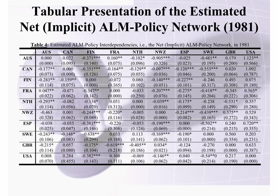
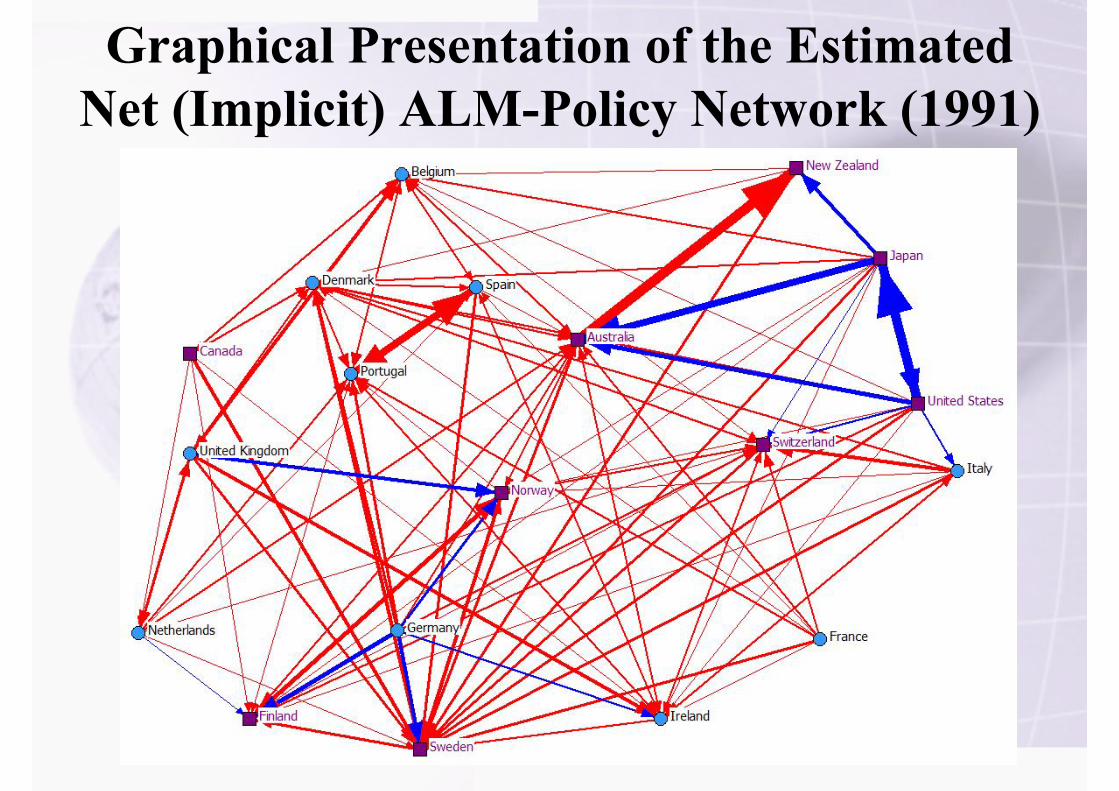
– Can even handle simultaneous estimation W and effect of W and even (we’re getting there) allowing some wij to be endogenous.
• Spatiotemporal Effects not directly read from coefficients: use graphs & response-plots & maps & grids
• S-T Coevolutionary Effects nonlinear in endogenous vars, so another order of difficulty, but nearly there too.
• Info-demands Galton’s Problem big, + Co-evolution uREALLY big. Only real option, at least for our goals, & at least where interdependence is appreciable:– Max effort to theory, measure, specification, & to both C&IPE.– Extant approaches that eschew such structural specification not
typically valid if (insofar as) interdep (appreciable): e.g., if S-interdependence then not SUTVA…
Presenting Effects: Some other Examples
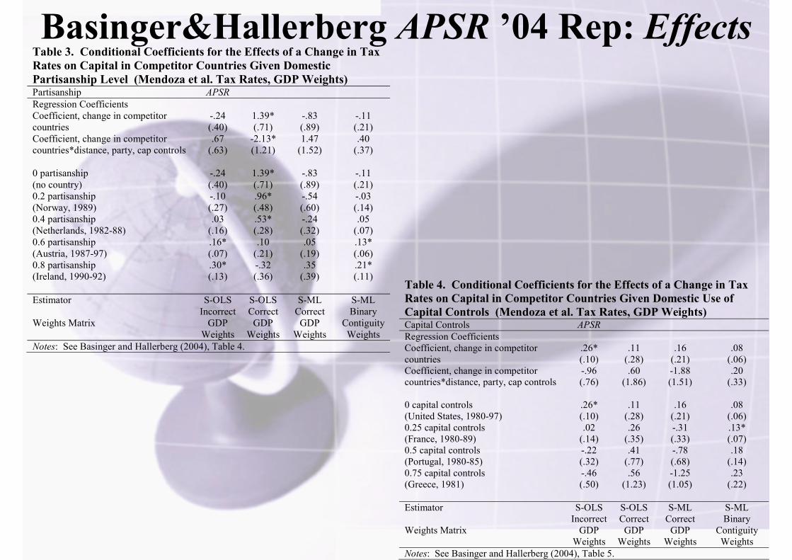
Basinger&Hallerberg APSR ’04 Rep: EffectsTable 2. Conditional Coefficients for the Effects of a Change in Tax Rates on Capital in Competitor Countries Given Domestic Ideological Distance (Mendoza et al. Tax Rates, GDP Weights) Ideological Distance APSR Regression Coefficients Coefficient, change in competitor countries
.24* (.12)
.38 (.28)
-.13 (.29)
.15* (.08)
Coefficient, change in competitor countries*distance, party, cap controls
Notes: See Basinger and Hallerberg (2004), Table 3.
Basinger&Hallerberg APSR ’04 Rep: EffectsTable 3. Conditional Coefficients for the Effects of a Change in Tax Rates on Capital in Competitor Countries Given Domestic Partisanship Level (Mendoza et al. Tax Rates, GDP Weights) Partisanship APSR Regression Coefficients Coefficient, change in competitor countries
-.24 (.40)
1.39* (.71)
-.83 (.89)
-.11 (.21)
Coefficient, change in competitor countries*distance, party, cap controls
.67 (.63)
-2.13* (1.21)
1.47 (1.52)
.40 (.37)
0 partisanship (no country)
-.24 (.40)
1.39* (.71)
-.83 (.89)
-.11 (.21)
0.2 partisanship (Norway, 1989)
-.10 (.27)
.96* (.48)
-.54 (.60)
-.03 (.14)
0.4 partisanship (Netherlands, 1982-88)
.03 (.16)
.53* (.28)
-.24 (.32)
.05 (.07)
0.6 partisanship (Austria, 1987-97)
.16* (.07)
.10 (.21)
.05 (.19)
.13* (.06)
0.8 partisanship (Ireland, 1990-92)
.30* (.13)
-.32 (.36)
.35 (.39)
.21* (.11)
Estimator S-OLS S-OLS S-ML S-ML Weights Matrix
Incorrect GDP
Weights
Correct GDP
Weights
Correct GDP
Weights
Binary Contiguity Weights
Notes: See Basinger and Hallerberg (2004), Table 4.
Table 4. Conditional Coefficients for the Effects of a Change in Tax Rates on Capital in Competitor Countries Given Domestic Use of Capital Controls (Mendoza et al. Tax Rates, GDP Weights) Capital Controls APSR Regression Coefficients Coefficient, change in competitor countries
.26* (.10)
.11 (.28)
.16 (.21)
.08 (.06)
Coefficient, change in competitor countries*distance, party, cap controls
-.96 (.76)
.60 (1.86)
-1.88 (1.51)
.20 (.33)
0 capital controls (United States, 1980-97)
.26* (.10)
.11 (.28)
.16 (.21)
.08 (.06)
0.25 capital controls (France, 1980-89)
.02 (.14)
.26 (.35)
-.31 (.33)
.13* (.07)
0.5 capital controls (Portugal, 1980-85)
-.22 (.32)
.41 (.77)
-.78 (.68)
.18 (.14)
0.75 capital controls (Greece, 1981)
-.46 (.50)
.56 (1.23)
-1.25 (1.05)
.23 (.22)
Estimator S-OLS S-OLS S-ML S-ML Weights Matrix
Incorrect GDP
Weights
Correct GDP
Weights
Correct GDP
Weights
Binary Contiguity Weights
Notes: See Basinger and Hallerberg (2004), Table 5.
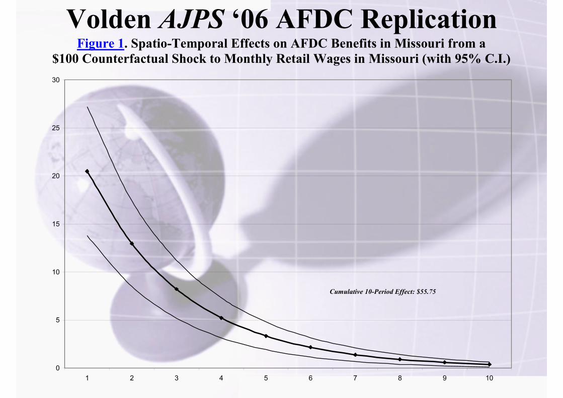
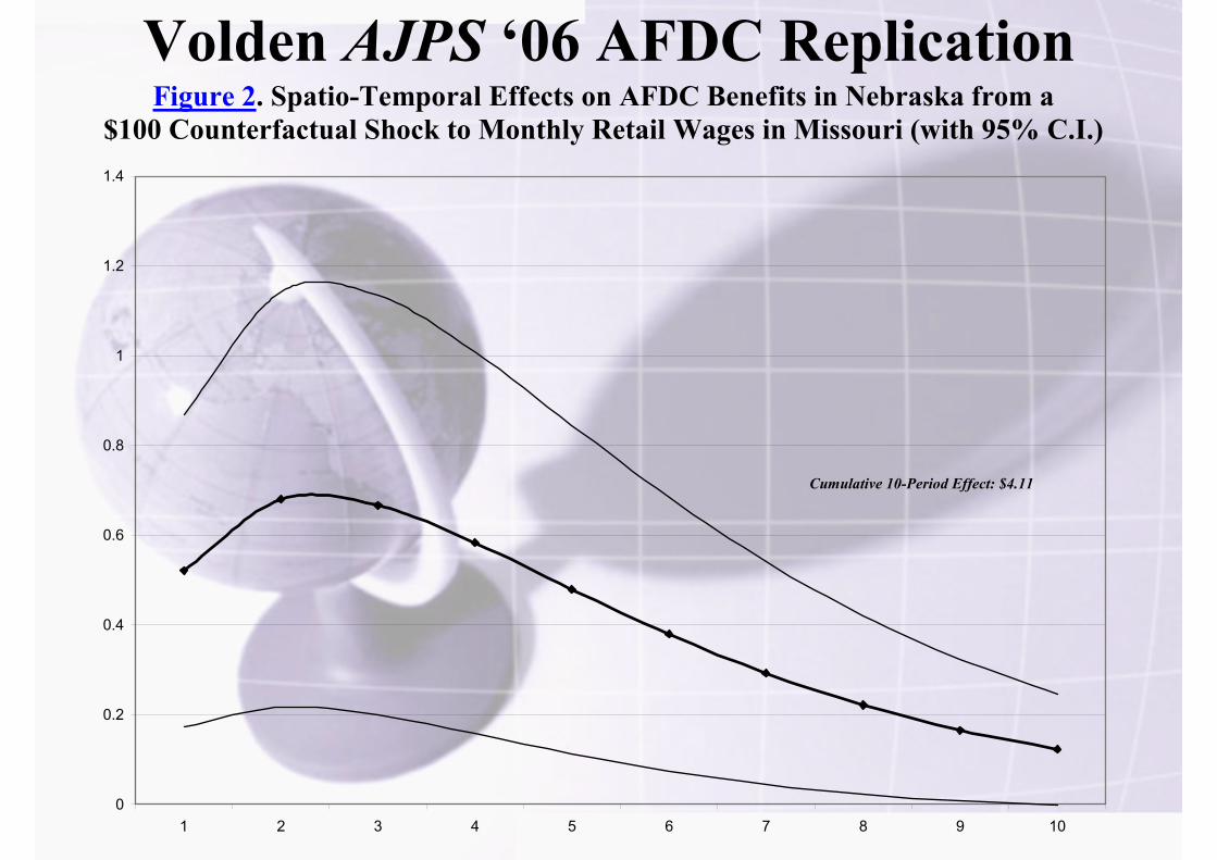
Volden AJPS ‘06 AFDC Rep: EffectsTable 4. Spatial Effects on AFDC Benefits from a $100 Counterfactual Shock to Monthly Retail Wages in Missouri Neighbor
Immediate Spatial Effect
Long-Run Steady State Effect
Arkansas
.51 [.16,.87]
4.26 [1.01,7.52]
Illinois
.62 [.19,1.04]
5.11 [1.25,8.97]
Iowa
0.52 [.15,.88]
4.37 [.99, 7.75]
Kansas
0.77 [.23,1.31]
6.38 [1.60,11.17]
Kentucky
0.44 [.13,.75]
3.68 [.87,6.50]
Nebraska
0.52 [.15,.89]
4.44 [.99,7.90]
Oklahoma
0.52 [.15,.89]
4.47 [.96,7.98]
Tennessee
0.38 [.12,.65]
3.21 [.75,5.67]
Notes: Effects calculated using estimates from the spatial AR lag model in Table 3. Brackets contain a 95% confidence interval.
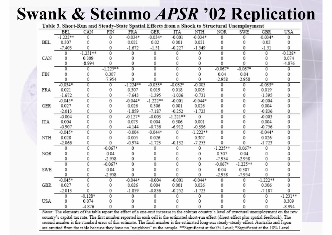
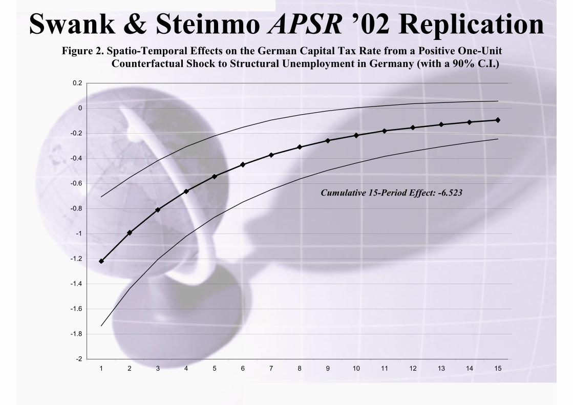
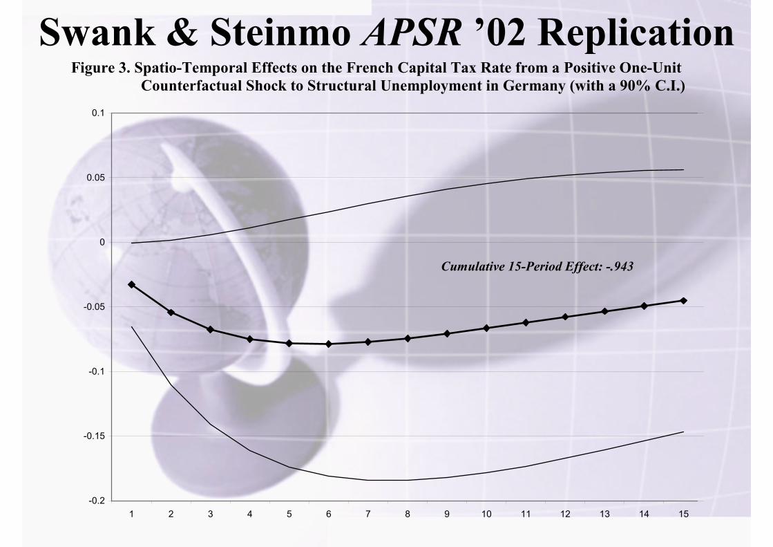
Swank & Steinmo APSR ’02 Replication
Swank & Steinmo APSR ’02 ReplicationFigure 2. Spatio-Temporal Effects on the German Capital Tax Rate from a Positive One-Unit
Counterfactual Shock to Structural Unemployment in Germany (with a 90% C.I.)
-2
-1.8
-1.6
-1.4
-1.2
-1
-0.8
-0.6
-0.4
-0.2
0
0.2
1 2 3 4 5 6 7 8 9 10 11 12 13 14 15
Cumulative 15-Period Effect: -6.523
Swank & Steinmo APSR ’02 ReplicationFigure 3. Spatio-Temporal Effects on the French Capital Tax Rate from a Positive One-Unit
Counterfactual Shock to Structural Unemployment in Germany (with a 90% C.I.)
-0.2
-0.15
-0.1
-0.05
0
0.05
0.1
1 2 3 4 5 6 7 8 9 10 11 12 13 14 15
Cumulative 15-Period Effect: -.943
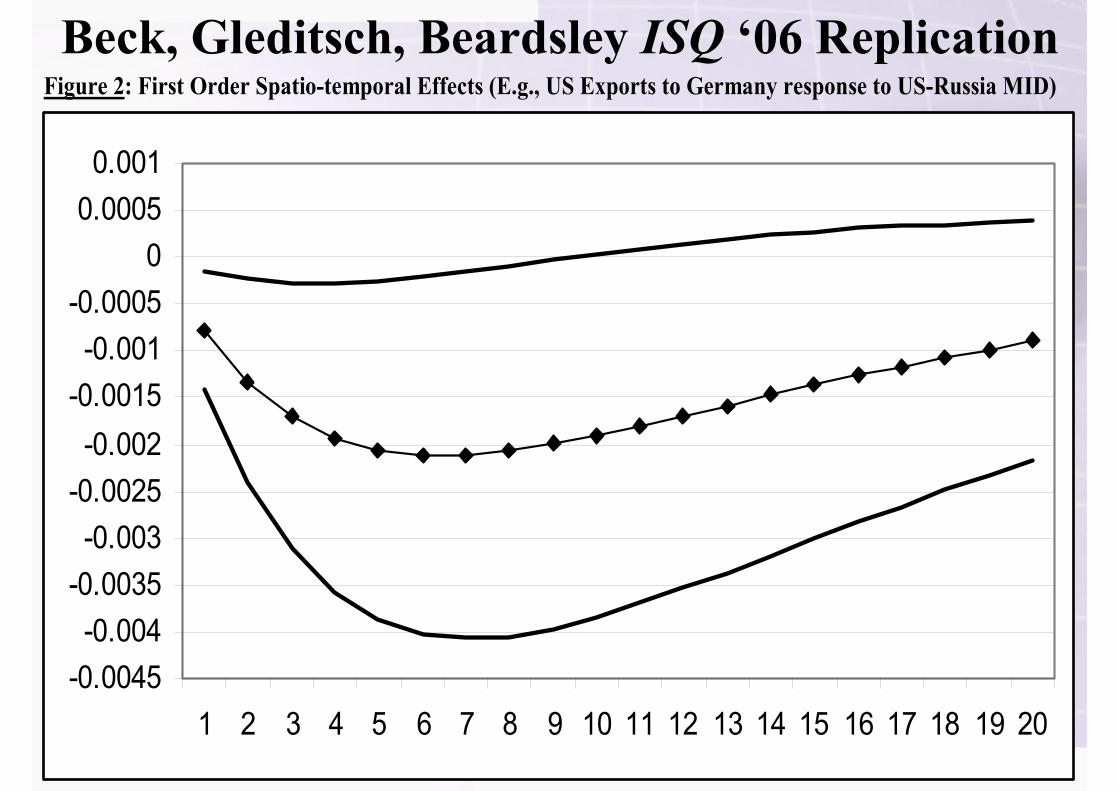
Beck, Gleditsch, Beardsley ISQ ‘06 Replication Figure 1: Temporal Effects with Spatial Feedback (E.g., US Exports to Russia response to US-Russia MID)
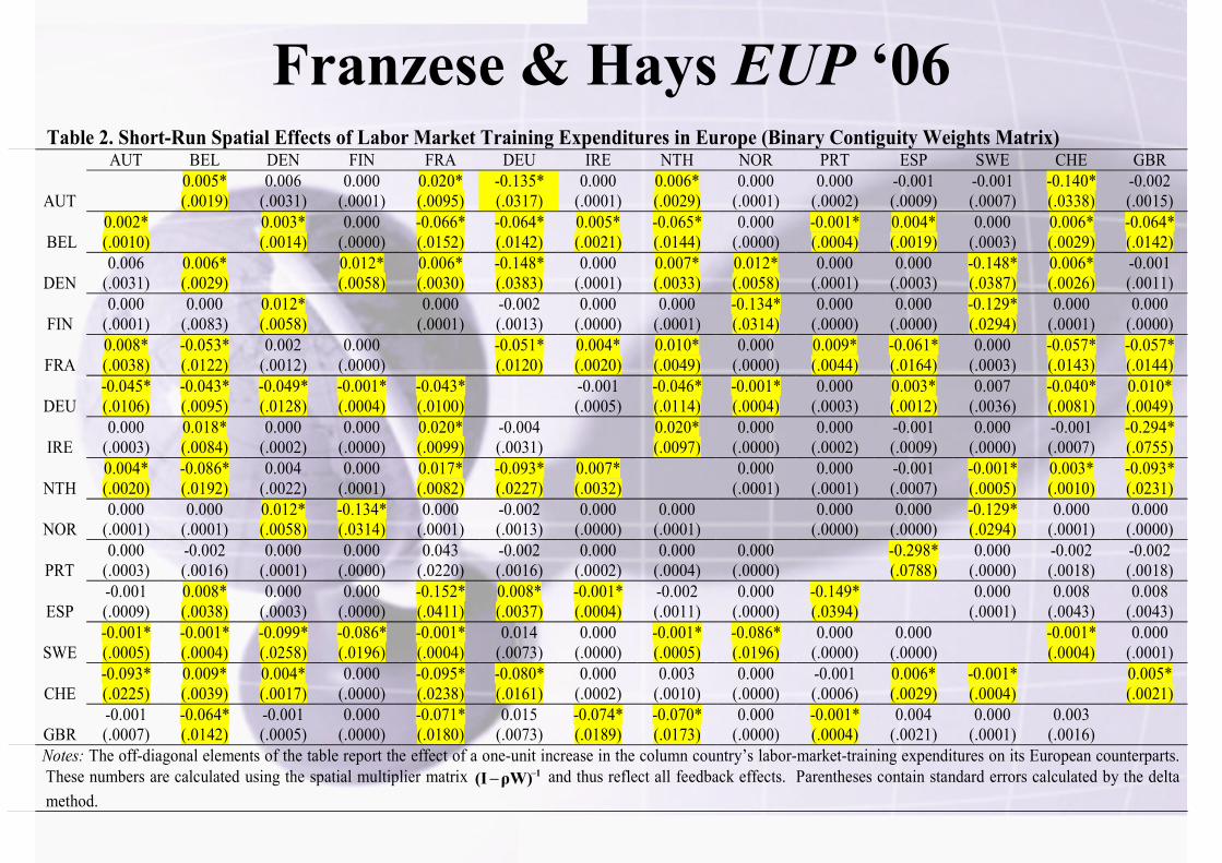
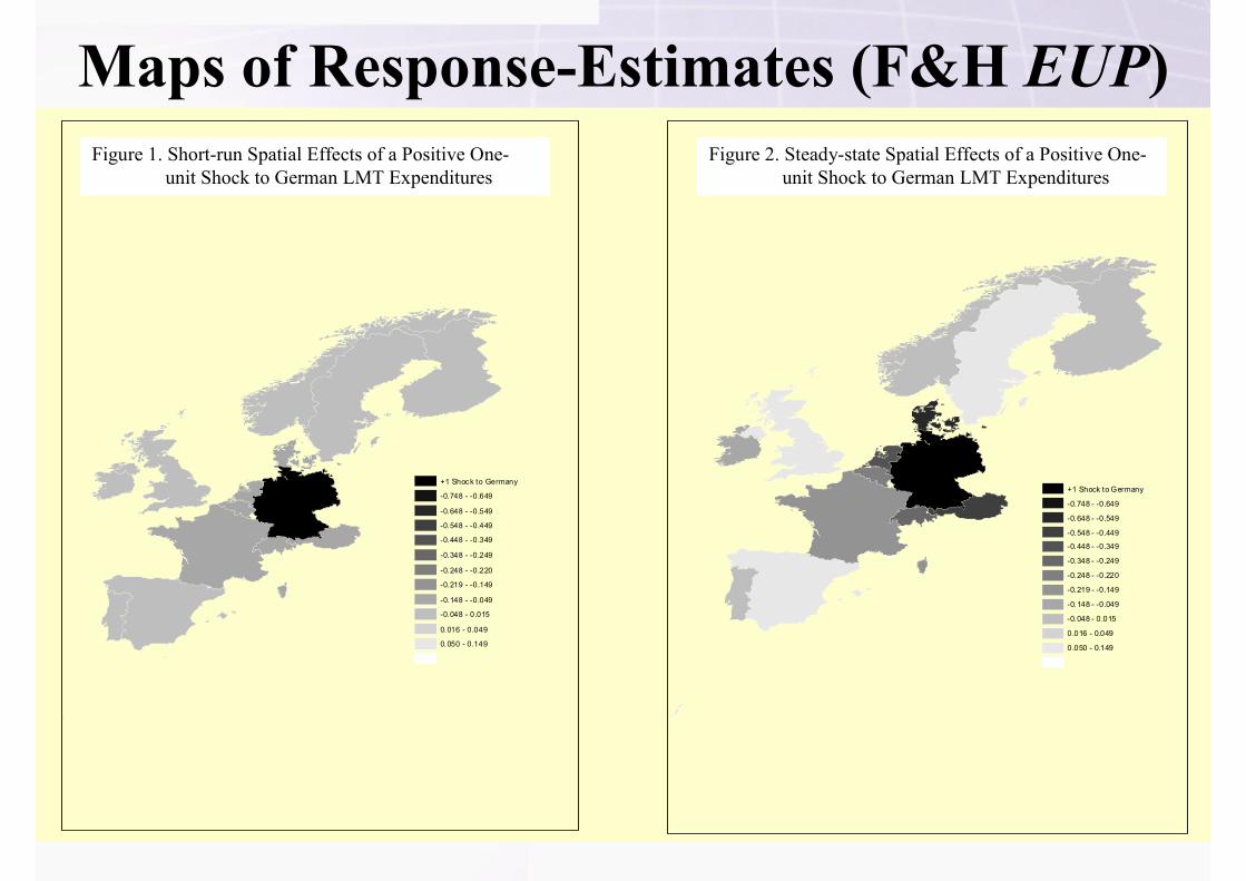
Franzese & Hays EUP ‘06 Table 2. Short-Run Spatial Effects of Labor Market Training Expenditures in Europe (Binary Contiguity Weights Matrix)
AUT BEL DEN FIN FRA DEU IRE NTH NOR PRT ESP SWE CHE GBR
AUT 0.005*
(.0019) 0.006
(.0031) 0.000
(.0001) 0.020* (.0095)
-0.135* (.0317)
0.000 (.0001)
0.006* (.0029)
0.000 (.0001)
0.000 (.0002)
-0.001 (.0009)
-0.001 (.0007)
-0.140* (.0338)
-0.002 (.0015)
BEL
0.002* (.0010)
0.003* (.0014)
0.000 (.0000)
-0.066* (.0152)
-0.064* (.0142)
0.005* (.0021)
-0.065* (.0144)
0.000 (.0000)
-0.001* (.0004)
0.004* (.0019)
0.000 (.0003)
0.006* (.0029)
-0.064* (.0142)
DEN
0.006 (.0031)
0.006* (.0029)
0.012* (.0058)
0.006* (.0030)
-0.148* (.0383)
0.000 (.0001)
0.007* (.0033)
0.012* (.0058)
0.000 (.0001)
0.000 (.0003)
-0.148* (.0387)
0.006* (.0026)
-0.001 (.0011)
FIN
0.000 (.0001)
0.000 (.0083)
0.012* (.0058)
0.000 (.0001)
-0.002 (.0013)
0.000 (.0000)
0.000 (.0001)
-0.134* (.0314)
0.000 (.0000)
0.000 (.0000)
-0.129* (.0294)
0.000 (.0001)
0.000 (.0000)
FRA
0.008* (.0038)
-0.053* (.0122)
0.002 (.0012)
0.000 (.0000)
-0.051* (.0120)
0.004* (.0020)
0.010* (.0049)
0.000 (.0000)
0.009* (.0044)
-0.061* (.0164)
0.000 (.0003)
-0.057* (.0143)
-0.057* (.0144)
DEU
-0.045* (.0106)
-0.043* (.0095)
-0.049* (.0128)
-0.001* (.0004)
-0.043* (.0100)
-0.001 (.0005)
-0.046* (.0114)
-0.001* (.0004)
0.000 (.0003)
0.003* (.0012)
0.007 (.0036)
-0.040* (.0081)
0.010* (.0049)
IRE
0.000 (.0003)
0.018* (.0084)
0.000 (.0002)
0.000 (.0000)
0.020* (.0099)
-0.004 (.0031)
0.020* (.0097)
0.000 (.0000)
0.000 (.0002)
-0.001 (.0009)
0.000 (.0000)
-0.001 (.0007)
-0.294* (.0755)
NTH
0.004* (.0020)
-0.086* (.0192)
0.004 (.0022)
0.000 (.0001)
0.017* (.0082)
-0.093* (.0227)
0.007* (.0032)
0.000 (.0001)
0.000 (.0001)
-0.001 (.0007)
-0.001* (.0005)
0.003* (.0010)
-0.093* (.0231)
NOR
0.000 (.0001)
0.000 (.0001)
0.012* (.0058)
-0.134* (.0314)
0.000 (.0001)
-0.002 (.0013)
0.000 (.0000)
0.000 (.0001)
0.000 (.0000)
0.000 (.0000)
-0.129* (.0294)
0.000 (.0001)
0.000 (.0000)
PRT
0.000 (.0003)
-0.002 (.0016)
0.000 (.0001)
0.000 (.0000)
0.043 (.0220)
-0.002 (.0016)
0.000 (.0002)
0.000 (.0004)
0.000 (.0000)
-0.298* (.0788)
0.000 (.0000)
-0.002 (.0018)
-0.002 (.0018)
ESP
-0.001 (.0009)
0.008* (.0038)
0.000 (.0003)
0.000 (.0000)
-0.152* (.0411)
0.008* (.0037)
-0.001* (.0004)
-0.002 (.0011)
0.000 (.0000)
-0.149* (.0394)
0.000 (.0001)
0.008 (.0043)
0.008 (.0043)
SWE
-0.001* (.0005)
-0.001* (.0004)
-0.099* (.0258)
-0.086* (.0196)
-0.001* (.0004)
0.014 (.0073)
0.000 (.0000)
-0.001* (.0005)
-0.086* (.0196)
0.000 (.0000)
0.000 (.0000)
-0.001* (.0004)
0.000 (.0001)
CHE
-0.093* (.0225)
0.009* (.0039)
0.004* (.0017)
0.000 (.0000)
-0.095* (.0238)
-0.080* (.0161)
0.000 (.0002)
0.003 (.0010)
0.000 (.0000)
-0.001 (.0006)
0.006* (.0029)
-0.001* (.0004)
0.005* (.0021)
GBR
-0.001 (.0007)
-0.064* (.0142)
-0.001 (.0005)
0.000 (.0000)
-0.071* (.0180)
0.015 (.0073)
-0.074* (.0189)
-0.070* (.0173)
0.000 (.0000)
-0.001* (.0004)
0.004 (.0021)
0.000 (.0001)
0.003 (.0016)
Notes: The off-diagonal elements of the table report the effect of a one-unit increase in the column country’s labor-market-training expenditures on its European counterparts. These numbers are calculated using the spatial multiplier matrix 1ρW)(I −− and thus reflect all feedback effects. Parentheses contain standard errors calculated by the delta method.