An O(n log n) algorithm for maximum st-flow in

a directed planar graph∗

Glencora Borradaile† Philip Klein‡

Abstract

We give the first correct O(n log n) algorithm for finding a maximumst-flow in a directed planar graph. After a preprocessing step that consistsin finding single-source shortest-path distances in the dual, the algorithmconsists of repeatedly saturating the leftmost residual s-to-t path.

1 Introduction

Informally, the maximum st-flow problem is as follows: given a graph withpositive arc-capacities, and given a source vertex s and a sink vertex t, thegoal is to find a way to route the maximum amount of a single commodityalong s-to-t paths in such a way that the amount of commodity passing throughan arc is at most the capacity of the arc. In the minimum st-cut problem, thegoal is to find a minimum-capacity set of arcs such that each s-to-t path includesat least one arc in the set. Formal definitions will be given in Section 4.5.

The history of maximum-flow and minimum-cut problems [32] is tied closelyto planar graphs. During the height of the cold war, the United States spent con-siderable effort analyzing the Soviet rail network: “The success of interdictiondepends largely on [the] interdiction-program efforts on the enemy’s capabilityto move men and supplies.” [16] Modeling the Soviet rail network as a planargraph (by taking the dual of the planar graph composed of boundaries of ad-ministrative districts with edges representing transportation capacity betweenthese districts), Harris and Ross, as members of the RAND corporation, studiedthe problem of determining the best way to interdict the Soviet rail network.That is, they found the minimum number of rail lines that must be cut in orderto stop movement of supplies and men between tactically important locations:they found a minimum cut in the graph. Ford and Fulkerson picked up on thisline of research, leading to their landmark paper proving the max-flow, min-cuttheorem and formulating the augmenting-path algorithm [11].

∗A preliminary version of this paper was published as [4].†Department of Combinatorics and Optimization, University of Waterloo. Work done while

at the Department of Computer Science, Brown University. Partially supported by the Roshfoundation, a PGS-D fellowship from NSERC, and NSF Grant CCF-0635089.

‡Department of Computer Science, Brown University. Partially supported by NSF GrantCCF-0635089.

1

Theorem 1.1 (Max-Flow Min-Cut). The value of the maximum st-flow is equalto the capacity of the minimum st-cut.

The Max-Flow Min-Cut Theorem was discovered independently by Ford andFulkerson [11], Kotzig [28], and Elias et al. [8].

2 Maximum flow algorithms

In the same paper that proved the Max-Flow Min-Cut Theorem, Ford andFulkerson suggested an algorithm (actually, a paradigm) for finding a maximumflow called the augmenting path algorithm. The algorithm is iterative: find apath P from the source to the sink and push flow on this path. The residualcapacity of an arc is the capacity less the flow on the arc. That is, the value ofthe flow for each dart in P is increased by an amount ∆ that does not exceedthe residual capacity of any arc on P . A formal description will be given inSection 4.5.

Dinitz [5] and Edmonds and Karp [7] showed that if the shortest (withrespect to number of arcs) augmenting path is chosen then there are at mostnm iterations. Dinitz gave an O(n2m) analysis for this using the notion of ablocking flow. In [14], Goldberg and Rao gave a clever implementation resulting

in an O(min(n2/3, m1/2)m log n2

m log U)-time algorithm (where U is the largestintegral capacity) by using a different, adaptive notion of distance that is relatedto the residual capacities. This is the fastest known algorithm for maximum flowin a general graph and results in an O(n3/2 log n log U)-time algorithm for planargraphs. For a more detailed survey see [13].

We briefly mention another type of maximum flow algorithm: the push-relabel algorithm, alternatively known as the preflow-push algorithm [15]. Ratherthan pushing flow along paths, flow is pushed on individual arcs. This algorithmdoes not maintain a feasible flow during its execution; it augments arcs in orderto bring the flow closer to feasibility.

3 History of planar maximum flow

In [11], Ford and Fulkerson gave a particular augmenting-path algorithm forthe case of finding the maximum st-flow in a planar graph in which the sourceand the sink are on the boundary of a common face, the infinite face. Such agraph is termed st-planar. With the graph viewed with the source embeddedon the left and the sink on the right, the algorithm iteratively augments (infact, saturates) the uppermost residual path. This algorithm has the propertythat the flow on an arc is never decreased. Since each augmentation makes atleast one arc non-residual, the algorithm requires at most m augmentations,where m is the number of arcs. In 1979, Itai and Shiloach [22] showed that eachiteration of the uppermost path algorithm could be implemented in O(log n)time, where n is the number of vertices, using a priority queue of the residual

2

darts. Consequently, the algorithm can be carried out in O(n log n) time (usingthe fact that a simple planar graph with n vertices has at most 3n arcs).

In 1981, Hassin demonstrated that a maximum st-flow in an st-planar graphG could be derived from shortest-path distances in the planar dual G∗ (see Sec-tion 4.3) of G where capacities in G are interpreted as lengths in G∗. With thisinsight, it can be seen that the uppermost-path algorithm can be interpretedin the planar dual as Dijkstra’s algorithm. The fact that the uppermost pathalgorithm can be implemented to run in O(n log n) time corresponds to the ob-servation, due to Johnson [23], that Dijkstra’s algorithm could be implementedto run in O(n log n) time by using a priority queue. Frederickson showed laterthat shortest-path distances in a planar graph with nonnegative lengths couldbe computed in O(n

√log n) time [12], and Henzinger et al. showed subsequently

that the same problem could be solved in O(n) time [21]. Combining this withHassin’s result yields an O(n)-time algorithm for maximum st-flow in st-planargraphs.

There remained, however, the more general and more natural problem ofst-flow in a planar graph in which s and t need not be on the boundary ofa common face. In 1983, Reif [30] showed that the minimum st-cut (and so,via the Max-Flow Min-Cut Theorem, also the value of the max st-flow) couldbe found in O(n log2 n) time for the special case of undirected planar graphs.This algorithm uses the observation that the edges crossing a min st-cut form aminimum length cycle C that separates s from t in the planar dual graph (wheres and t are faces). The algorithm finds a shortest path P in the planar dual froma vertex incident to s to a vertex incident to t. Reif proves that C only crosses Ponce. A divide-and-conquer algorithm is given in which a minimum separatingcycle is found that contains the middle edge e of P : this cycle correspondsto a min cut in the primal separating the endpoints of e. This results in anO(n log2 n)-time algorithm, using the aforementioned O(n log n) st-planar flowalgorithm of Itai and Shiloach. In 1985, Hassin and Johnson [18] drew on Reif’stechnique to show that the flow assignment could also be found within the sametime bound, again for undirected planar graphs. The shortest-path algorithms ofHenzinger et al. [21] or Klein [27] can be used to re-implement these algorithmsin O(n log n) time.

Still the more general problem of st-flow in a planar directed graph remainedopen. This problem is more general since the problem of maximum st-flow inan undirected graph can be converted to a directed problem by introducing twooppositely oriented arcs of equal capacity for each edge. In 1982, Johnson andVenkatesan gave a divide-and-conquer algorithm that finds a flow of input valuev in a directed planar graph in O(n1.5 log n) time [24]. The algorithm dividesthe graph using an O(

√n)-balanced separator, and recursively finds a flow in

each side of value v. The flow on the O(√

n)-boundary edges of each subproblemmight not be feasible; each boundary edge is made feasible via an st-planar flowcomputation.

In 1989, Miller and Naor [29] showed that finding a maximum st-flow canbe reduced to a sequence of shortest-path computations in a graph with pos-itive and negative lengths. In 2001, Fakcharoenphol and Rao [10] presented

3

an O(n log3 n) algorithm for the latter problem, implying an O(n log3 n logC)bound on maximum flow where C is the sum of the integral capacities.

Year Restriction Time Reference

1956 st-planar O(n2) Ford and Fulkerson [11]1979 st-planar O(n log n) Itai and Shiloach [22]1982 fixed value O(n

√n log n) Johnson and Venkatesan [24]

1983 value

undirected O(n log2 n) Reif [30]

1985 undirected O(n log2 n) Hassin and Johnson [18]1987 st-planar O(n

√log n) Hassin [17] using

Frederickson [12]1997 st-planar O(n) Hassin [17] using

Henzinger et al. [21]1997 undirected O(n log n) Hassin and Johnson [18] using

Henzinger et al. [21]

2001 O(n log3 n log C) Miller and Naor [29] usingFakcharoenphol & Rao [10]

Table 1: Planar Maximum-Flow and Minimum-Cut Algorithms

3.1 Toward an O(n log n) algorithm

In 1994, Weihe [36] published an O(n log n) algorithm for planar directed maxi-mum st-flow. The algorithm, though perhaps influenced by Ford and Fulkerson’suppermost-path algorithm, is quite different. From the example included in hispaper, it is clear that an augmenting path is not necessarily an uppermost path(as generalized to non-st-planar graphs). The algorithm and proof of correctnessare quite complicated.

In a preprocessing step of the algorithm, the input graph is transformed intoone satisfying the following three requirements.

1. Each vertex but the source and sink has degree exactly three;

2. there are no clockwise cycles; and

3. each arc uv belongs to a simple s-to-v path and a simple u-to-t path.

Satisfying Requirement 1 involves: splicing together every two successive arcssharing an endpoint of total degree two; and replacing each vertex of high degreeby a cycle, increasing the number of vertices to 2m, which is at most 6n. Re-quirement 2 can be satisfied by using a reduction of Khuller, Naor, and Klein [26]to computing shortest-path distances in the dual (and so can be computed inO(n) time using the algorithm of Henzinger et al. [21]). Details of this step willbe given in Section 5.1.

Requirement 3 is problematic. Weihe states “To satisfy this assumption,simply remove all arcs that violate it. None of these arcs will help us solve

4

our problem.” However, as pointed out by Biedl, Brejova, and Vinar [3], thereis no known O(n log n)-time algorithm to delete all such arcs. They give thebest known algorithm to date, which runs in O(n2) time. To our knowledge,the dependence of Weihe’s proof of correctness on Requirement 3 has not beenresolved. Although Weihe has claimed that his algorithm can be corrected, thishas not been verified.

4 Preliminaries

4.1 Graphs

Let G be a directed graph with arc-set A. For each arc a ∈ A, we define twooppositely directed darts, one in the same orientation as a (which we sometimesidentify with a) and one in the opposite orientation.

We define rev (·) to be the function that takes each dart to the correspond-ing dart in the opposite direction. Formally, the dart set is A × {±1}, andrev (〈a, i〉)) = 〈a,−i〉. The head and tail of a dart d in a graph G (writtenheadG(d) and tailG(d)) are such that the dart is oriented from tail to head. Wemay omit the subscript when doing so introduces no ambiguity. We may useuv to indicate a dart d such that u = tail(d) and v = head(d) when there is noambiguity due to parallel darts.

Walks, Paths and Cycles

A nonempty x-to-y walk is a nonempty sequence of darts d1 . . . dk such thatheadG(d1) = x, tailG(dk) = y and, for i = 2, . . . , k, headG(di−1) = tailG(di).The walk is said to contain a vertex if the vertex is the head or tail of one of thedarts making up the walk. The start vertex of the walk is defined to be the tailof d1, and the end vertex is defined to be the head of dk. We denote the startand end vertices of a walk W by start(W ) and end(W ), respectively. An emptywalk W is specified by a single vertex v such that start(W ) = end(W ) = v.

A walk in which no dart appears more than once is a path. If in additionheadG(dk) = tailG(d1) then the path is a cycle. A path/cycle of darts is simpleif no vertex occurs twice as the head of a dart in the path/cycle. A path/cycleis said to be directed if each of its darts has the same orientation as the corre-sponding arc. We use the term undirected when we wish to emphasize that apath/cycle need not be directed. A graph or subgraph is connected if for everypair u, v of vertices it contains an undirected u-to-v path.

Subpaths and path concatenation

For a walk W containing vertices u and v, W [u, v] denotes the u-to-v subwalkof W . (If u or v occurs more than once in W , we will use this notation onlywhen it is clear which occurrence is intended.) If W is a cycle, W [u, v] denotesa subpath of the cycle.

5

W [·, v] is shorthand for W [start(W ), v], and W [u, ·] is shorthand for W [u, end(W )].We use W [u, v) to denote the walk obtained from W [u, v] by deleting the lastdart; W (u, v] and W (u, v) are defined similarly. The reverse of W = d1 . . . dk,denoted by rev (W ), is the walk rev (dk) rev (dk−1) . . . rev (d1).

If P = d1 . . . dk and Q = e1 . . . eℓ are walks such that end(P ) = start(Q), weuse P ◦ Q to denote the walk d1 . . . dke1 . . . eℓ.

Subgraphs

A subgraph H of a graph G is identified with a subset of arcs.A spanning tree T of G is a connected subgraph of G that contains all

vertices of G and contains no undirected simple cycle. For vertices u and v,T [u, v] denotes the unique (undirected) u-to-v path through T .

If a vertex of T is designated as a root, we use T [u] to denote the u-to-rootpath in T . Let xy be an edge of T where T [x] includes y. Then the correspondingdart, oriented from x to y, is called the parent dart of x in T .

For a graph G and a set S of vertices of G, δ+

G(S) is the set of darts whosetails are in S and whose heads are not. (We omit the subscript when the choiceof graph is clear from the context.) Such a set of darts is called a cut. A cut isa simple cut if both S and V \ S are connected. A simple cut is also known asa bond.

4.2 Vector spaces

The arc space of a graph G = 〈V, A〉 is the vector space RA: a vector δ in arcspace assigns a real number δ[a] to each arc a ∈ A. It is notationally convenientto interpret a vector δ in arc space as assigning real numbers to all darts. Fora dart 〈a, i〉 (i = ±1), we define

δ[〈a, i〉] = i · δ[a].

That is, if d is a dart in the same direction as the corresponding arc a thenδ[d] = δ[a], and if d points in the opposite direction then δ[d] = −δ[a].

For each arc a, we define δ(a) to be the vector in arc space that assigns 1 toa and zero to all other arcs:

∀a′ ∈ A, δ(a)[a′] =

{

1 if a′ = a,0 otherwise.

For a multi-set S of darts, we define δ(S) =∑

d∈S δ(d).The cycle space of G is the subspace of the arc space spanned by

C = {δ(C) : C a cycle of darts in G}.

We will refer to vectors in cycle space alternatively as circulations.

6

4.3 Planar graphs

According to the geometric definition, a planar graph is a graph for which thereexists a planar embedding. A planar embedding of a graph is a drawing of thegraph on the plane (or the surface of a sphere) so that vertices are mappedto distinct points and edges are mapped to non-crossing curves. A face is aconnected component in the set of points that are not in the image of any arcor vertex. For a connected graph embedded on the plane, there is one infiniteface. For a connected graph embedded on the sphere, an arbitrary face can bedesignated as the infinite face. We denote the infinite face by f∞.

One can alternatively define embeddings combinatorially, without referenceto topology [19, 6, 38]. A combinatorial embedding is sometimes called a rotationsystem. A combinatorial embedding is given by a permutation π such that foreach dart d, π(d) is the dart e such that x = tail(d) = tail(e) and e is thedart immediately after d in the counterclockwise ordering of the darts aroundx. While such a formulation frequently makes the implementation of algorithmssimpler, we will only use the permutation π explicitly in a few places throughoutthis work. However, we note that for all the algorithms contained herein, acombinatorial embedding is sufficient for implementation.

Duals of planar graphs

Corresponding to every connected planar embedded graph G there is anotherconnected planar embedded graph denoted G∗. The faces of G are the verticesof G∗ and vice versa. The arcs (and hence darts) of G correspond one-to-onewith those of G∗. If d is a dart of G, the tail of the corresponding dart of G∗

is the face to the left of d, and the head is the face to the right of d. Thusintuitively the geometric orientation in G∗ of the dart corresponding to d isobtained by rotating the embedding of d clockwise roughly 90 degrees. It isnotationally convenient to equate the darts of G with the darts of G∗. We callG the primal graph and G∗ the dual. An example is given in Figure 1. Therotation system for the combinatorial embedding of G∗ is denoted π∗ and isequal to π ◦ rev.

The boundary of a face f of a planar embedded graph is the cycle consistingof darts whose tail in the planar dual is f , ordered according to the cycle of π∗

corresponding to f . Figure 1 gives an example. We denote the boundary of fby ∂f . The boundary of the planar embedded graph G is denoted by ∂G and isdefined to be the boundary of its infinite face. According to our convention, fora face f other than the infinite face, ∂f is oriented counterclockwise, and ∂f∞is oriented clockwise.

We will liberally use the following two classical results on planar graphs.These theorems are illustrated in Figures 2 and 3, respectively.

Theorem 4.1 (Interdigitating Spanning Trees [9, 34]). For a spanning tree Tof G, the set of arcs not in T form a spanning tree of the dual G∗.

We denote the set of arcs not in T by T ∗.

7

a

bc

d

Figure 1: A planar graph and its dual: the primal is given by solid vertices andsolid arcs and the dual is given by open vertices and dotted arcs. The boundaryof one of the faces is the cycle a rev (b) c d.

Figure 2: The primal is given by solid arcs and the dual by dotted arcs. Thedark bold edges form a spanning tree T of the primal. The edges not in T forma spanning tree T ∗ of the dual.

Theorem 4.2 (Cycle-Cut Duality [37]). In a connected planar graph, a set ofdarts forms a simple directed cycle in the primal iff it forms a simple directedcut in the dual.

Circulations

Recall that the cycle space of G is the subspace of the arc space spanned byC = {δ(C) : C a cycle of darts in G}. Recall that ∂f consists of the dartsmaking up the boundary of face f . In a connected planar graph, the set ofvectors

{δ(∂f) : f a face of G, f 6= f∞}is a basis for the cycle space of G. Therefore, any vector η ∈ C can be representedas a linear combination of these basis vectors. We use φ to denote the vector ofcoefficients for this linear combination, so

η =∑

f 6=f∞

φ[f ]δ(∂f)

8

Figure 3: The primal is given by solid edges and the dual by dotted edges.The dark bold (directed) darts form a simple directed cycle in the dual and adirected bond, δ+(S), in the primal, where S is the set of the lower 4 vertices.

We call φ a potential assignment, and we refer to φ[f ] as the potential of face f .This use of potentials was introduced by Hassin [17] for st-planar graphs, andby Miller and Naor [29] for general planar graphs. We adopt the conventionthat φ[f∞] = 0.

Encloses

For a simple cycle C with a geometric embedding, we can say that C strictlyencloses a dart, vertex or face if the dart, vertex or face is embedded inside Cwith respect to f∞. We formalize this definition for any cycle C (not necessarilysimple).

Let C be a cycle and let φ be the potential corresponding to the circulationδ(C). Cycle C encloses a face f if φ[f ] 6= 0. Cycle C strictly encloses a dartd if C encloses the faces to the left and right of d (tailG∗(d) and headG∗(d),respectively). Cycle C encloses a dart d if C strictly encloses d, d ∈ C orrev (d) ∈ C. Cycle C encloses or strictly encloses a vertex v if C encloses orstrictly encloses, respectively) all the darts incident to v.

Clockwise and Counterclockwise

A circulation is defined as counterclockwise (abbreviated c.c.w.) if the potentialof every face is nonnegative [26]. A circulation is defined as clockwise (abbre-viated c.w.) if the potential of every face is non-positive. A directed cycle Cof darts is clockwise if δ(C) is clockwise. A cycle or circulation may be neithercounterclockwise nor clockwise, but a simple cycle is either clockwise or coun-terclockwise. These definitions have geometric interpretations, as illustrated byFigure 4.

For any face f , the boundary of f is a clockwise cycle if f 6= f∞ and acounterclockwise cycle if f = f∞.

9

(a) (b)

Figure 4: (a) A clockwise cycle. (b) A cycle that is neither clockwise norcounterclockwise.

a

b

d

Figure 5: The dart d enters the path a ◦ b from the right because d does notappear among the sequence of darts in counterclockwise order between b andrev (a).

Entering and Crossing

The notions of entering and crossing are illustrated in Figures 5 and 6.Suppose a, b, and d are darts such that head(a) = tail(b) = head(d): we say

d enters a ◦ b at head(a). If in addition rev (d) is not among b, π(b), π(π(b)), . . . ,πk(b)=rev (a) then d is said to enter a ◦ b from the right at head(a). (SeeFigure 5.) A path that contains d is said to enter a walk that contains a◦b fromthe right. Enters from the left, leaves from the right, etc., are defined similarly.

Suppose paths P and Q are such that R is a maximal common subpath ofP and Q. We say that P crosses Q if

• P enters Q from the right at start(R) and P leaves Q from the left atend(R), or

• P enters Q from the left at start(R) and P leaves Q from the right atend(R).

If P and Q are paths that do not cross, then they are non-crossing. Apath/cycle is non-self-crossing if for every pair P and Q of subpaths of thepath, P does not cross Q. Note that, for any face f , the boundary of f is anon-self-crossing cycle.

We will use the following lemma in Section 6 where we will use non-self-crossing cycles (simple cycles are not sufficiently general). This lemma allowsus to build non-self-crossing cycles from other non-self-crossing cycles.

10

PQ

x

y

(a)

P

Q

(b) (c)

v

(d)

Figure 6: (a) P crosses Q: P enters Q on the right at x and P leaves Q on theleft at y. (b) P and Q are non-crossing. (c) This is a self-crossing cycle. (d)This is a non-self-crossing but non-simple cycle, since vertex v occurs twice.

Lemma 4.3 (Composition Lemma). Let C be a non-self-crossing cycle and letA be a non-self-crossing path with endpoints on C such that no part of A isenclosed by C. Then

A ◦ C[end(A), start(A)]

is a non-self-crossing cycle.

Proof. Since no part of A is enclosed by C, A does not cross C. It follows thatA ◦ C[end(A), start(A)] is non-self-crossing.

4.4 Clockwise and leftmost

An x-to-y walk A is left of an x-to-y walk B if δ(A)−δ(B) is a clockwise circu-lation. (This definition was given by [27] for paths, but generalizes naturally towalks.) Likewise A is right of B if δ(A)−δ(B) is a counterclockwise circulation.Left of and right of are transitive, reflexive, antisymmetric relations. An x-to-ypath A is the leftmost x-to-y path in a graph if, for every x-to-y path B, A isleft of B. There is not necessarily a leftmost walk: suppose P = Q ◦ C is theleftmost path where Q is an x-to-y path and C is a c.w. cycle; then R = P ◦C isa walk that is left of P and R ◦C is left of R and so on. However, the followinglemma allows us to consider only simple paths when we are considering graphswith no clockwise cycles.

Lemma 4.4. Let G be a graph with no clockwise cycles. If P is a leftmost walk,then P is a simple path.

Proof. Assume for a contradiction that P is not a simple path. Let x be avertex that occurs at least twice on P . Let x1 be the first occurrence of x on Pand let x2 be the last. Then C = P [x1, x2] is a cycle. Since G has no clockwise

11

cycles, C must be counterclockwise. Let P ′ = P [·, x1]◦P [x2, ·] be the path thatis obtained from P by removing C. The circulation

δ(P ) − δ(P ′) = δ(C)

is counterclockwise, so P is strictly right of P ′. Thus P is not leftmost, acontradiction.

Lemma 4.5. Every subpath of a leftmost path is a leftmost path.

Proof. Let P be a leftmost path. Let Q be an x-to-y subpath of P . Supposethere is another x-to-y path Q′ 6= Q that is left of Q. Let P ′ = P [·, x]◦Q′◦P [y, ·].The circulation

δ(P ′) − δ(P ) = δ(P [·, x] ◦ Q′ ◦ P [y, ·]) − δ(P [·, x] ◦ Q ◦ P [y, ·])= δ(Q′) − δ(Q)

is clockwise since Q′ is left of Q. So P ′ 6= P is left of P , a contradiction.

Theorem 4.6 (Non-Crossing Theorem). If P and Q are disjoint non-self-crossing x-to-y paths that do not cross each other, then P is either right ofor left of Q.

Proof. Let C = Q◦ rev (P ): C is a non-self-crossing cycle. Let GC be the graphconsisting of the edges and vertices of C. Since GC is a connected graph, eachface of GC has a connected boundary. We show that δ(C) is either a clockwiseor counterclockwise circulation.

We claim that each face of GC uses either darts of C or darts of rev (C) (butnot both). Suppose for a contradiction that f is a face that uses darts of bothC and rev (C). Let A and B be maximal subpaths of C such that A ∈ ∂f andrev (B) ∈ ∂f and end(A) = start(rev (B)). Let A′ and B′ be the subpaths ofC such that C = A ◦ A′ ◦ B ◦ B′. Since f is a face, C does not cross ∂f andso A ◦ A′ must leave ∂f from the left (at end(A), by the maximality of A).Likewise, B ◦ B′ leaves ∂f from the left. Since C is non-self-crossing, A ◦ A′

does not cross B ◦ B′. However B′ is an end(B)-to-start(A) path and A′ is aend(A)-to-start(B), so A′ crosses B′, a contradiction, proving the claim. SeeFigure 7 for an illustration.

Consider the following assignment of numbers to faces.

φ[f ] =

{

−1 if ∂f ⊂ C0 if rev (∂f) ⊂ C

By the claim, every face is assigned a number.If φ[f∞] = 0, then φ is a valid potential assignment and corresponds to the

circulation η = δC. Then C is clockwise and Q is left of P .If φ[f∞] = −1, then φ + 1 is a valid potential assignment (where 1 is the

all-ones vector). It follows that C is counterclockwise and Q is right of P .

12

B

B'

A

A'

f

Figure 7: If A ◦ A′ ◦ B ◦ B′ is a cycle and A ∪ rev (B) ∈ ∂f , then A′ must crossB′.

4.5 Maximum flows and minimum cuts

We now give the formal statement of the maximum-flow and minimum-cut prob-lems. Given a graph G, a source vertex s, a sink vertex t, and an assignmentc(·) of real-valued capacities to the arcs of G, the maximum-flow problem is asfollows:

max f · δ(δ+({s}))s.t. f is a vector in arc-space (1)

f · δ(δ+({v})) = 0, ∀v ∈ V \ {s, t} (2)

0 ≤ f [a] ≤ c(a), ∀ arcs a (3)

Constraint (2) is the conservation constraint: the net flow at every non-source-or-sink vertex is zero. Constraint (3) is the capacity constraint.

A flow assignment f or st-flow is called feasible if it satisfies these constraints.The goal is to maximize the value of the flow, f · δ(δ+({s})). A flow of valuezero is called a circulation and is a vector in cycle space.

Given the same input, the minimum st-cut problem is:

min c(δ+(S))

s.t. s ∈ S ⊆ V \ {t} (4)

A set of vertices S satisfying Constraint (4) is called an st-cut. The value of acut is given by the objective function.

The capacity function c(·) assigns capacities to arcs. We extend it to dartsas follows: c(〈a, 1〉) = c(a) and c(〈a,−1〉) = 0 for each arc a. That is, a dart inthe same direction as the corresponding arc has the same capacity as the arc,and a dart in the opposite direction has capacity zero.

A flow f assigns values to arcs. We extend it to darts as follows: f [〈a, 1〉] =f [a] and f [〈a,−1〉] = −f [a].

For any flow f , the residual capacity of a dart d, written cf (d), is c(d)− f [d].A dart d is residual with respect to f and c if its residual capacity is positive.

Otherwise, d is non-residual. A path is residual if all its darts are residual.

13

It follows from the Max-Flow Min-Cut Theorem that a feasible st-flow f ismaximum if and only if there is no residual s-to-t path with respect to f and c.Augmenting an st-flow f along a residual s-to-t path P , means increasing f [d]by the same amount for each dart d in P . We call this path the augmentingpath. Suppose that f is feasible with respect to c. If the amount of the increaseis no more than

∆ = mind∈P

c(d) − f [d],

then after augmentation the st-flow f is still feasible. If the increase is exactly∆, then we say the augmentation saturates the path P . In this case, at leastone dart of P becomes saturated (i.e., non-residual).

5 The max-flow algorithm

We present an algorithm to find a maximum st-flow in a directed planar graphthat runs in O(n log n) time. The algorithm is a direct generalization of theuppermost-path algorithm. Ford and Fulkerson’s algorithm finds the upper-most flow: one in which no flow can be rerouted above the existing flow. Ourgeneralization finds the leftmost flow (which we define in the next section, and isdefined with respect to the infinite face). At the start of the algorithm, we startwith a leftmost flow of value zero, which is achieved via a preprocessing stepequivalent to satisfying Requirement 2 of Weihe’s algorithm. The algorithm,which we call MaxFlow, is as follows:

• Designate a face incident to t as f∞.

• Saturate the clockwise cycles. (LeftmostCirculation)

• While there is a residual s-to-t path, saturate the leftmost suchpath. (LeftmostFlow)

In Section 5.1, we review an algorithm due to Khuller, Naor, and Klein [26]for carrying out the second step, LeftmostCirculation. This algorithm waspreviously used by Weihe [36]. In Section 5.2, we discuss the third step, Left-

mostFlow. We state a theorem, the Unusability Theorem, that implies thatthe third step, LeftmostFlow, takes O(n) iterations. We give an implementa-tion in which each iteration takes O(log n) time. (More precisely, the implemen-tation allows for some degenerate iterations in which zero flow is pushed, butthe Unusability Theorem enables us to show that the total number of iterationsis nevertheless linear.) In Section 6, we prove the Unusability Theorem.

5.1 LeftmostCirculation

The second step of the MaxFlow algorithm, LeftmostCirculation, is im-plemented using the following algorithm, due to Khuller, Naor, and Klein [26]. It

14

computes an assignment of potentials to the faces using single-source shortest-path distances in the dual planar graph, interpreting capacities as distances.(We denote the length of the shortest x-to-y path in G as distG(x, y).)

LeftmostCirculation(G), c(·), f∞)

• Interpret capacities c(d) as lengths of darts in the dual graph G∗.• Let φ[f ] = distG∗(f, f∞) for every face f .• Let η[d] = φ[tailG∗(d)] − φ[headG∗(d)] for every dart d.• Return η.

Lemma 5.1 (Khuller et al. [26]). The graph has no clockwise cycle that isresidual with respect to the circulation returned by LeftmostCirculation.

Proof. Let C be a clockwise cycle of darts in G and let T be the tree representingthe shortest-path distances computed in LeftmostCirculation. There is apath in T to f∞ from every face enclosed by C, so at least one dart of C is inthe shortest-path tree. Let d be such a dart:

cη(d) = c(d) − η[d]

= c(d) − (distG∗(tailG∗(d), f∞) − distG∗(headG∗(d), f∞))

= c(d) − c(d) since d is in the shortest-path tree

= 0

Since d is not residual, the cycle C is not residual.

5.2 LeftmostFlow

Weihe [36] defined a leftmost maximum st-flow. We slightly generalize this. Wesay an st-flow f (not necessarily maximum) is a leftmost flow if the residualgraph with respect to f has no clockwise residual cycles.

Lemma 5.2. Let f be a leftmost flow and let P be the leftmost residual path.The flow f ′ that results from saturating P is a leftmost flow.

Proof. Assume for a contradiction that f ′ is not a leftmost flow. By the defini-tion of leftmost, there must then be a clockwise residual cycle C with respect tof ′. Assume w.l.o.g. that C is simple. Since f was leftmost, C was not residualprior to the augmentation, and so P must have a dart d in common with rev (C).

Let P ′ = P [·, tail(d)]◦C[tail(d), tail(d)]◦P [tail(d), ·] where C[tail(d), tail(d)]is the clockwise cycle starting at tail(d). P ′ is a walk and δ(P ′) − δ(P ) =δ(P ) + δ(C) − δ(P ) = δ(C) is a clockwise circulation and so P ′ is left of P .Therefore P was not the leftmost residual path.

Next we discuss the third step of our MaxFlow algorithm, Leftmost-

Flow: starting with the circulation η output by the second step (Leftmost-

Circulation), repeatedly saturate the leftmost residual s-to-t path until noneremains. It is convenient for the analysis to describe LeftmostFlow as an

15

algorithm that takes as input a new graph G0 and new capacity function c0(·),derived from the original input graph Gin and capacity function cin(·), thatsatisfies the following preconditions.

Precondition 5.3. G0 has no clockwise cycle of arcs.

Precondition 5.4. For every arc a in G0, c0(a) > 0.

To obtain G0 and c0(·) from the original input graph Gin and original capac-ity function cin(·) in the MaxFlow algorithm, we use the leftmost circulationη found in the second step. For each dart of Gin that is residual with respectto η, we include a corresponding arc in G0, and we assign the residual capacityof the dart as the capacity of the new arc in G0. Because Gin has no cycle ofdarts that is residual with respect to η, G0 satisfies Precondition 5.3. Becauseeach arc in G0 arises from a residual dart, G0 satisfies Precondition 5.4.

The algorithm LeftmostFlow finds a maximum st-flow f in G0. By addingη to f , we obtain a maximum st-flow in the original graph Gin.

However, it should be emphasized that this distinction between the inputgraph Gin and G0 is purely for notational convenience; it enables the analysisto use the term arc to refer to a dart that is residual with respect to the left-most circulation. A simpler and equivalent version of LeftmostFlow wouldsimply continue working with the input graph Gin using the circulation foundby LeftmostCirculation as the initial flow assignment.

We start with an abstract version of LeftmostFlow.

(Abstract) LeftmostFlow(G0, c0, s, t, f∞)

• Initialize f = 0.• While there is an s-to-t path that is residual w.r.t. f and c0, sat-

urate the leftmost residual s-to-t path, modifying f .• Return f .

The following invariant of LeftmostFlow follows from Lemma 5.2:

Invariant 5.5. During the execution of LeftmostFlow, G0 has no clockwiseresidual cycles with respect to f .

Corollary 5.6. During the execution of LeftmostFlow, there is no cycle ofdarts all assigned positive flow.

Proof. Assume for contradiction that C is a cycle of darts all assigned positiveflow. If C is counterclockwise, then rev (C) is residual, contradicting Invari-ant 5.5. If C is clockwise, then C contradicts Precondition 5.3.

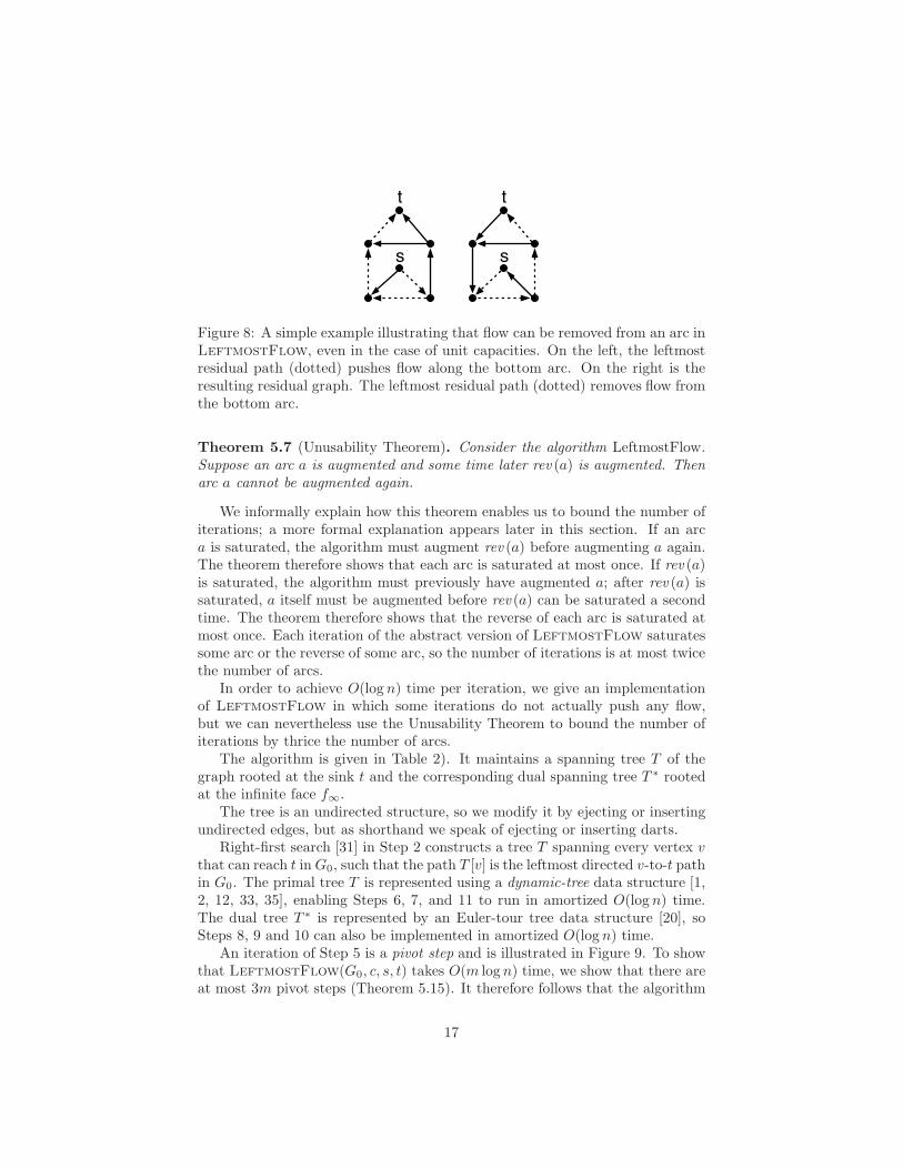
In Ford and Fulkerson’s uppermost-path algorithm for st-planar graphs, onceflow is pushed on an arc, flow can never be removed from that arc. For planargraphs that are not st-planar, such a strong property does not hold, as illustratedin Figure 8. However, we prove a weaker property that suffices for the analysis.

16

s

t

s

t

Figure 8: A simple example illustrating that flow can be removed from an arc inLeftmostFlow, even in the case of unit capacities. On the left, the leftmostresidual path (dotted) pushes flow along the bottom arc. On the right is theresulting residual graph. The leftmost residual path (dotted) removes flow fromthe bottom arc.

Theorem 5.7 (Unusability Theorem). Consider the algorithm LeftmostFlow.Suppose an arc a is augmented and some time later rev (a) is augmented. Thenarc a cannot be augmented again.

We informally explain how this theorem enables us to bound the number ofiterations; a more formal explanation appears later in this section. If an arca is saturated, the algorithm must augment rev (a) before augmenting a again.The theorem therefore shows that each arc is saturated at most once. If rev (a)is saturated, the algorithm must previously have augmented a; after rev (a) issaturated, a itself must be augmented before rev (a) can be saturated a secondtime. The theorem therefore shows that the reverse of each arc is saturated atmost once. Each iteration of the abstract version of LeftmostFlow saturatessome arc or the reverse of some arc, so the number of iterations is at most twicethe number of arcs.

In order to achieve O(log n) time per iteration, we give an implementationof LeftmostFlow in which some iterations do not actually push any flow,but we can nevertheless use the Unusability Theorem to bound the number ofiterations by thrice the number of arcs.

The algorithm is given in Table 2). It maintains a spanning tree T of thegraph rooted at the sink t and the corresponding dual spanning tree T ∗ rootedat the infinite face f∞.

The tree is an undirected structure, so we modify it by ejecting or insertingundirected edges, but as shorthand we speak of ejecting or inserting darts.

Right-first search [31] in Step 2 constructs a tree T spanning every vertex vthat can reach t in G0, such that the path T [v] is the leftmost directed v-to-t pathin G0. The primal tree T is represented using a dynamic-tree data structure [1,2, 12, 33, 35], enabling Steps 6, 7, and 11 to run in amortized O(log n) time.The dual tree T ∗ is represented by an Euler-tour tree data structure [20], soSteps 8, 9 and 10 can also be implemented in amortized O(log n) time.

An iteration of Step 5 is a pivot step and is illustrated in Figure 9. To showthat LeftmostFlow(G0, c, s, t) takes O(m log n) time, we show that there areat most 3m pivot steps (Theorem 5.15). It therefore follows that the algorithm

17

(Implementation) LeftmostFlow(G0, c0, s, t)

1. Initialize f = 0.2. Initialize T to be the right-first search tree searching backwards

from t. (Every arc in T is directed towards t.)3. Let G be the graph obtained from G0 by deleting all vertices not

in T .4. Initialize T ∗ to consist of the edges of G∗ that are not in T .5. Repeat:

6. If T [s] is residual, saturate T [s], modifying f .7. Let d be the last non-residual dart in T [s].8. If tailG∗(d) is a descendent in T ∗ of headG∗(d), return f .9. Let e be the parent dart in T ∗ of headG∗(d).

10. Eject e from T ∗ and insert d into T ∗.11. Eject d from T and insert e into T .

Table 2: A network-simplex type implementation of the LeftmostFlow algo-rithm.

runs in O(m log n) time.First we show that the algorithm does maintain spanning trees of G and G∗.

Invariant 5.8. T is a spanning tree of G and T ∗ is a spanning tree of G∗.

Proof that the algorithm maintains the invariant. Initially, Step 2 establishesthat T is a spanning tree of G and Step 4 establishes that T ∗ is a spanningtree of G∗, by the Interdigitating Spanning Trees Theorem. Ejecting e fromT ∗ in Step 10 breaks T ∗ into two connected component, one consisting of thedescendents of headG∗(d) in T ∗ and one consisting of the non-descendents. Atthe time Step 10 is about to be executed, the condition in Step 8 is false, sotailG∗(d) is not a descendent of headG∗(d) in T ∗. It follows that in T ∗ insertingd joins the two connected components, so T ∗ is a spanning tree of G∗ at theend of Step 10. By the Interdigitating Spanning Trees Theorem, therefore, T isa tree of G after Step 11. 2

Note that Step 11 can result in reversing parent and child in some edges.Specifically, as illustrated in Figure 9, the path in T between tailG(d) andtailG(e) is reversed. However, this is within the scope of the dynamic-tree datastructure.

Invariant 5.9. Let e be an edge of T ∗, and let d be the corresponding dart thatis oriented away from f∞. Then d is non-residual.

Proof that the algorithm maintains the invariant. First we show that the in-variant holds initially. T ∗ is composed of edges not in T . Let a be any arc not inT . By construction of T , the path of arcs a◦T [headG(a)] is right of T [tailG(a)].

18

Before

d

e

t

s

f∞ After

Figure 9: The edges of T are solid, non-tree edges are dashed. The root of T isthe sink t. T ∗ is represented by light edges, and its root is the infinite face f∞.In an iteration of LeftmostFlow, the s-to-t path is saturated and d is therootmost non-residual edge. The shaded face is headG∗(d). This face’s parentdart e in T ∗ is ejected from T ∗ and inserted into T , and rev (d) is inserted intoT ∗ and becomes the new parent dart. The edge that immediately precedes d inthe s-to-t path gets reversed: the parent endpoint becomes the child endpointand vice versa.

Let C = a ◦T [headG(a), tailG(a)]. Then C is a simple c.c.w. cycle. The face tothe left of a is enclosed by C and the face to the right is not. Let S be the setof faces enclosed by C. In G∗, a is directed out of S (i.e. a ∈ δ+

G∗(S)). Sincea is the only arc in C that is not in T and therefore is in T ∗, and since f∞ isnot enclosed by C, 〈a, 1〉 is directed towards f∞ in T ∗ and 〈a,−1〉 is orientedaway from f∞. Since the reverses of arcs have zero capacity, the invariant holdsinitially.

See Figure 9 for an illustration of the next argument. Note that, in eachnonterminating pivot step, tailG∗(d) is not a descendent in T ∗ of headG∗(d).Dart e, the parent of headG∗(d), is removed from T ∗. The component of T ∗−{e}that contains f∞ contains tailG∗(d) and not headG∗(d), so when d is insertedinto T ∗, d is oriented away from f∞. Since d was saturated in Step 6, d isnon-residual.

Let c be a dart that remains in T ∗ during a pivot. The residual capacity ofc does not change and the orientation of c in T ∗ does not change. Therefore theinvariant holds. 2

We say that a dart d is a non-tree dart if the corresponding edge is not in T .

Lemma 5.10. There is no clockwise simple cycle whose non-tree darts are allresidual.

Proof. Suppose for a contradiction that C was such a cycle. Let S be theset of non-tree darts in C. By Invariant 5.8, for every dart d ∈ S, the treeT ∗ contains the edge corresponding to d. Since every dart in S is residual,

19

Invariant 5.9 implies that in T ∗ the darts of S are oriented towards the rootf∞. Since C is clockwise, headG∗(d) is enclosed by C for every dart d in C.Since T is a tree, C contains at least one non-tree dart d. The directed pathT ∗[headG∗(d)] is completely enclosed by C, implying that C also encloses f∞ =end(T ∗[headG∗(d)]), a contradiction.

We show in the next two corollaries that the network-simplex version of Left-

mostFlow implements the abstract version. Corollary 5.11 shows that everyaugmentation is along the leftmost residual s-to-t path and Corollary 5.12 showsthat the algorithm does not terminate until there is no s-to-t residual path.

Corollary 5.11. For every vertex v, there is no residual path strictly left ofT [v].

Proof. Suppose for a contradiction that there is a residual path strictly left ofT [v]. Then the leftmost residual v-to-t path P must be strictly left of T [v]. LetQ be a subpath of P such that the endpoints of Q are on T [v] but Q and rev (Q)are both edge disjoint from T [v]. Since P is leftmost, by Lemma 4.5, Q is leftof T [end(Q), start(Q)], so Q ◦ rev (T [end(Q), start(Q)]) is a simple c.w. cyclewhose non-tree darts are residual, contradicting Lemma 5.10.

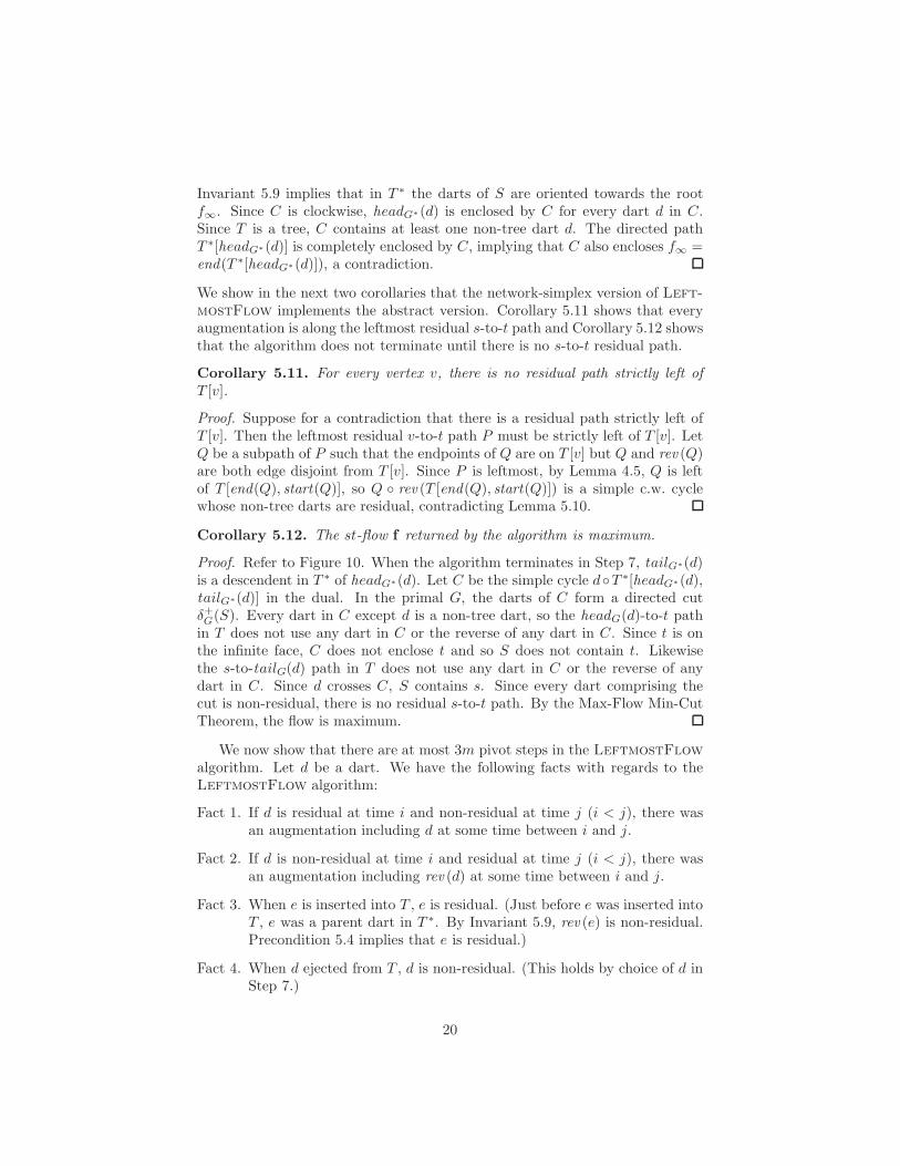
Corollary 5.12. The st-flow f returned by the algorithm is maximum.

Proof. Refer to Figure 10. When the algorithm terminates in Step 7, tailG∗(d)is a descendent in T ∗ of headG∗(d). Let C be the simple cycle d◦T ∗[headG∗(d),tailG∗(d)] in the dual. In the primal G, the darts of C form a directed cutδ+

G(S). Every dart in C except d is a non-tree dart, so the headG(d)-to-t pathin T does not use any dart in C or the reverse of any dart in C. Since t is onthe infinite face, C does not enclose t and so S does not contain t. Likewisethe s-to-tailG(d) path in T does not use any dart in C or the reverse of anydart in C. Since d crosses C, S contains s. Since every dart comprising thecut is non-residual, there is no residual s-to-t path. By the Max-Flow Min-CutTheorem, the flow is maximum.

We now show that there are at most 3m pivot steps in the LeftmostFlow

algorithm. Let d be a dart. We have the following facts with regards to theLeftmostFlow algorithm:

Fact 1. If d is residual at time i and non-residual at time j (i < j), there wasan augmentation including d at some time between i and j.

Fact 2. If d is non-residual at time i and residual at time j (i < j), there wasan augmentation including rev (d) at some time between i and j.

Fact 3. When e is inserted into T , e is residual. (Just before e was inserted intoT , e was a parent dart in T ∗. By Invariant 5.9, rev (e) is non-residual.Precondition 5.4 implies that e is residual.)

Fact 4. When d ejected from T , d is non-residual. (This holds by choice of d inStep 7.)

20

s

td

rev(d)

Figure 10: An illustration of Corollary 5.12. Darts of the dual tree are dark,with darts of T ∗ solid. In the dual, s and t are faces, shown shaded. Upontermination, tailG∗(d) is a descendent in T ∗ of headG∗(d). Since rev (d) is non-residual and the reverses of dual tree darts are non-residual, the cycle shown isa saturated cut separating s from t. The darts of this cut (in the primal) arelight.

Claim 5.13. A dart 〈a, 1〉 where a is an arc of G0 is ejected at most once.

Proof. Let a be an arc and let d = 〈a, 1〉. Suppose for a contradiction that a isejected at time i1 and at time i2 (i1 < i2).

To be ejected at time i1, d must be non-residual by Fact 4. Fact 1 impliesthat there was an augmentation including d at some time k0 where 0 < k0 < i1.

To be ejected at time i2, d must have been inserted at some time j1 wherei1 < j1 < i2. At time j1, d is residual by Fact 3. By Fact 2, there was anaugmentation including rev (d) at some time k1 where i1 < k1 < j1.

Since there was an augmentation including d at time k0 and there was anaugmentation including rev (d) at time k1 > k0, d cannot be augmented aftertime k1 by the Unusability Theorem.

Finally, to be ejected at time i2, d must be non-residual by Fact 4. By Fact2, there was an augmentation including d at some time k2 where j1 < k2 < i2.But d cannot be augmented after time k1. This is a contradiction.

Corollary 5.14. A dart 〈a,−1〉 where a is an arc of G0 is ejected at mosttwice.

Proof. Let a be an arc and let d = 〈a,−1〉.Suppose d is ejected at times i1 and i2. Then d must be inserted at time

i1 < j1 < i2. By Fact 4, d is non-residual at time i1 and by Fact 3, d is residualat time j1. By Fact 2, rev (d) must be part of an augmentation at some time k1

where i1 < k1 < j1.Likewise, by Fact 4, d is non-residual at time i2 and by Fact 1 d must be

augmented at time k2 where j1 < k2 < i2.At time i2, d is out of the tree and non-residual. Since rev (d) cannot be

augmented after time k2 by Claim 5.13, d can never become residual again andso cannot be inserted or ejected again.

As a consequence of the above, we have the following theorem:

21

Theorem 5.15. There are at most 3m pivot steps in the LeftmostFlow

algorithm.

6 Unusability Theorem

In this section, we prove the Unusability Theorem. The structure of the proof isas follows. We show that if an arc a is augmented and later rev (a) is aug-mented, then a structure in the residual graph arises called an obstruction(Lemma 6.11). We show that this structure persists under leftmost augmen-tations (Lemma 6.12). We also prove (Lemma 6.10) that the existence of theobstruction ensures that no leftmost residual path includes arc a, which showsthat a is never augmented again.

The idea of the proof is as follows. We assume for a contradiction thatthe leftmost residual path A does include a. We use a suffix of the s-to-tail(a)subpath of A together with paths comprising the obstruction to construct a cycleC such that the arc a is completely enclosed by C, as shown in Figure 16(b),and we show that the head(a)-to-s subpath of A cannot escape from this cycle(escaping would imply that an invariant failed to hold).

We make use of Preconditions 5.3 (no c.w. cycles) and 5.4 (every arc isinitially residual). We will use the term arc to refer to an arc of G0 (and to thecorresponding dart), and use anti-arc to refer to a dart whose reverse is an arc.

Before commencing the proof, we establish some properties of leftmost resid-ual paths and walks. Recall that since the graphs we consider have no clockwiseresidual cycles (Invariant 5.5), the leftmost walk is a simple path (Lemma 4.4).

Lemma 6.1 (Prohibited augmentations). The following situations are not per-mitted if A is a leftmost augmentation and the given vertex indices are well-defined:

1. A[x, y] is right of a residual walk R[x, y].

2. A[x, y] makes a clockwise cycle with residual walk R[y, x].

3. A has a dart that enters a t-to-s residual walk R from the right.

Proof. We prove each part separately.

1. A[s, x] ◦R[x, y] ◦A[y, t] is left of A. This contradicts the requirement thatA is leftmost residual walk.

2. This contradicts Invariant 5.5.

3. Suppose uv is a dart of a leftmost augmentation path and suppose uventers a t-to-s residual walk R from the right. As such, uv /∈ R andrev (uv) /∈ R. A[s, u] must intersect R at some vertex: let x be the lastintersection of A[s, u] with R (possibly x = s). If x ∈ R(v, s], then A[x, v]◦R[v, x] is clockwise, contradicting Invariant 5.5. If x ∈ R(t, v) then R[x, v]is a residual walk that is left of A[x, v], which is a prohibited augmentationof the first kind.

22

Now we define what it means to be unusable. Unusability is given by astructure in the residual graph called an obstruction.

Definition 6.2 (Unusable Arc). An obstruction is a clockwise non-self-crossingcycle L ◦ M where L is residual and M consists entirely of arcs. We say it isan obstruction for an arc a if 〈a, 1〉 is the first dart of L. We say an arc a isunusable if there is an obstruction for a.

We give a second, equivalent representation for an obstruction which will beuseful in proving the Unusability Theorem. Both are illustrated in Figure 11.

M

(a)

Q2

Q1

R

(b)

Figure 11: (a) An obstruction for arc a as given by Definition 6.2. (b) Theobstruction for arc a as given by Lemma 6.3 with the obstruction from (a)shaded in the background. L, Q2 and R are residual; M , Q1 and Q2 consist ofarcs; a is the first arc of L and Q2.

Lemma 6.3. A clockwise non-self-crossing cycle C satisfies Definition 6.2 iffit can be written as Q1 ◦ Q2 ◦ R where

1. Q1 ◦ Q2 consists entirely of arcs,

2. Q2 ◦ R is residual,

3. a is the first dart of Q2,

4. there is flow through the vertex start(R), and

5. there is flow through the vertex end(R).

Proof. The “if” direction is trivial. To prove the “only if” direction, let L ◦ Mbe an obstruction for a. Since G0 has no clockwise cycle of arcs, L ◦ M cannotconsist entirely of arcs. Let b be the first anti-arc of L. By Invariant 5.5, L ◦Mcannot consist entirely of residual darts and so M cannot consist entirely ofresidual darts. Let c be the first non-residual dart of M .

Let Q1 = M [tail(c), ·], let Q2 = L[·, tail(b)], and let R = L[tail(b), ·] ◦M [·, tail(c)]. By choice of b, L[·, tail(b)] consists entirely of arcs, so property 1holds. By choice of c, M [·, tail(c)] is residual, so property 2 holds. Since a isthe first dart of L, property 3 holds. Since b is a residual anti-arc, rev (b) carriesflow, so property 4 holds. Since c is a non-residual arc, by Precondition 5.4 itcarries flow, so property 5 holds.

23

Definition 6.4. For an unusable arc a, let ∆a denote the obstruction for a thatencloses the minimum number of faces (breaking ties arbitrarily). Write ∆a asQ1

a ◦ Q2a ◦ Ra, and let Qa denote Q1

a ◦ Q2a.

Considering a minimally enclosing obstruction simplifies the proofs becauseit allows us to rule out the existence of certain paths that cross the obstruction.Let C be a non-self-crossing cycle, and let P be a path whose start and end arevertices of C. If P has at least one dart, we say P crosscuts C if every dart ofP is strictly enclosed by C. If P has no darts (i.e. start(P ) = end(P )), we sayP crosscuts C if start(P ) occurs more than once in C. Note that in either casethe path P splits C into two cycles, e.g. containing strictly fewer faces.

A non-trivial path P is a flow path if every dart of P is assigned a positiveflow value. A trivial path P (i.e. having no darts) is a flow path if there is adart incident to start(P ) that is assigned a positive flow value. Note that adart assigned a positive flow value must correspond to an arc, i.e. cannot be ananti-arc.

Property 6.5. Suppose a is unusable. There is no residual path crosscutting∆a from a vertex in Q2

a(·, ·] to a vertex in Q1a.

Proof. Assume for a contradiction that W is such a residual path. Then W ◦Q1

a[end(W ), ·] ◦ Q2a[·, start(W )] is an obstruction for arc a that encloses fewer

faces than ∆a does. That is, W can be used to replace Ra in the obstruction.

Property 6.6. Suppose a is unusable. Q2a belongs to a t-to-s residual path.

Proof. Since ∆a is a clockwise cycle, it cannot be residual, so Q1a cannot be

residual. Let b be the last non-residual dart of Q1a. Since Q1

a contains only arcs,b carries flow and this flow must be routed to t. Let Ft be any head(b)-to-t flowpath and let Fs be any s-to-start(Ra) flow path. Since the reverse of a flow pathis residual, the path rev (Ft) ◦ Q1

a[head(b), ·] ◦ Q2a ◦ rev (Fs) is a residual t-to-s

path.

Property 6.7. There are no flow paths that crosscut ∆a.

Proof. Assume for contradiction that F is such a flow path, and assume withoutloss of generality that F is simple. Let α = start(F ) and β = end(F ). ThenC1 = ∆a[α, β] ◦ rev (F ) and C2 = F ◦ ∆a[β, α] are clockwise non-self-crossingcycles, each enclosing fewer faces than ∆a. See Figure 12.

We will refer to the following:

Argument 1 Note that rev (F ) is residual. If ∆a[α, β] were residual then C1

would be a residual clockwise cycle, contradicting Invariant 5.5.Since all non-residual darts of ∆a are in Q1

a, we infer that ∆a[α, β]must include at least one dart of Q1

a.

Argument 2 Note that F consists entirely of arcs. If ∆a[β, α] consisted entirelyof arcs then C2 would be a clockwise cycle of arcs in G0, contra-dicting Precondition 5.3. Since all anti-arcs of ∆a are in Ra, weinfer that ∆a[β, α] must include at least one dart of Ra.

24

C1

C2

∆a

α

β

F

(a)

α

β

F

R

Q1

Q2

(b)

α

β

F

R

Q1

Q2

(c)

α

β F

R

Q1

Q2

(d)

Figure 12: Property 6.7 (a) An illustration of the cycles C1 and C2 for the theproof of Property 6.7. By Argument 1, there is an arc (bold) of Q1

a in ∆a[α, β].By Argument 2, there is an arc (grey) of Ra in ∆a[β, α]. (b) Case 1, first sub-case. C1 is a smaller obstruction. (c) Case 1, second sub-case. C2 is a smallerobstruction. (d) Case 2. C1 is a smaller obstruction.

There are two cases to consider:

Case 1 start(Ra) is a vertex of ∆a[β, α]: By Argument 1, Q1a is not a subpath

of ∆a[β, α]. If a is in ∆a[α, β] then C1 is an obstruction enclosing fewerfaces than ∆a (Figure 12b). If a is in ∆a[β, α] then C2 is an obstructionenclosing fewer faces than ∆a (Figure 12c).

Case 2 start(Ra) is a vertex of ∆a(α, β): By Argument 2, Ra is not a subpathof ∆a[α, β], so end(Ra) is outside ∆a[α, β]. By Argument 1, Q1

a is nota subpath of ∆a[β, α], so α is a vertex of Q1

a. Therefore the first arc ofQ2

a, which is a, is in ∆a[α, β], so C1 is an obstruction enclosing fewerfaces than ∆a (Figure 12d).

Each case contradicts the minimality condition of ∆a.

Corollary 6.8. If ∆a strictly encloses a flow-carrying dart d, then ∆a strictlyencloses the source s and every s-to-head(d) flow path.

Proof. Suppose for a contradiction that there is a flow-carrying dart d strictlyenclosed by ∆a and an s-to-head(d) flow path P containing a dart e that is not

25

strictly enclosed by ∆a. Let Q be a head(d)-to-t flow path. The path P ◦ Qcontains a subpath that starts at a vertex (head(e)) not strictly enclosed by ∆a,goes through a dart (d) strictly enclosed by ∆a, and ends at a vertex (t) notstrictly enclosed by ∆a. Such a flow path violates Property 6.7.

For an unusable arc a, there is a start(Ra)-to-t flow path and an s-to-end(Ra)flow path by Parts 4 and 5 of Lemma 6.3.

Corollary 6.9. For an unusable arc a, any start(Ra)-to-t flow path does notintersect any s-to-end(Ra) flow path.

Proof. Let Ft be any start(Ra)-to-t flow path and let Fs be any s-to-end(Ra)flow path. By Corollary 5.6, each of these paths is simple. Suppose for acontradiction that Ft and Fs share a vertex. Let w be the first such vertexin Ft. See Figure 13. Let F ′

s be the maximal suffix of Fs that is not strictlyenclosed by ∆a. By Corollary 6.8, F ′

s is the only part of Fs that is not strictlyenclosed by ∆a. Since Ft ends at a vertex that is not strictly enclosed by ∆a,Property 6.7 implies that no arc of Ft is strictly enclosed by ∆a, so w must bea vertex of F ′

s.Let F = Ft[start(Ra), w] ◦Fs[w, end(Ra)]. F is a start(Ra)-to-end(Ra) flow

path that is not internal to ∆a. By the Non-Crossing Theorem, F is either rightof or left of Ra. There are two cases.

Case 1 If F is right of Ra, Ra◦rev (F ) is a clockwise residual cycle, contradictingInvariant 5.5.

Case 2 If F is left of Ra, F is also left of rev (Qa) by transitivity. Hence F ◦Qa

is a clockwise cycle in G0, a contradiction. This case is illustrated inFigure 13.

Qa

Ft

w

Ra

Fs

s

Figure 13: If flows to and from ∆a (dashed), Fs and Ft, share a vertex w, thenwe can construct from them a start(Ra)-to-end(Ra) flow path F (bold). Theshaded area is bounded by a clockwise cycle of arcs.

26

Now we have all the tools needed to prove the Unusability Theorem. We proveit in three parts. First we show that an unusable arc cannot belong to a leftmostresidual path (Lemma 6.10). Next we show that if an arc a satisfies the condi-tion of the Unusability Theorem, there is an obstruction for a in the residualgraph (Lemma 6.11). Finally we show that obstructions persist under leftmostaugmentations (Lemma 6.12). The Unusability Theorem follows.

R

Q1

Q2

s

Fs

A1

a

Figure 14: Lemma 6.10, construction of C1. The obstruction ∆a is shown inbold. It consists of paths R, Q1, and Q2, where a is the first arc of Q2. Thes-to-end(Ra) flow path Fs is indicated by a solid line. The dashed curve A1

denotes a subpath of a leftmost residual path A that is assumed to include thearc a. The interior of the cycle C1 is shaded.

Lemma 6.10 (Unusable Arc Consequence). A leftmost augmenting path con-tains no unusable arcs.

Proof. Let A be the leftmost augmenting path, and assume for a contradictionthat it goes through an unusable arc a.

The goal is to first construct a non-self-crossing cycle C that strictly enclosesa and does not enclose t. A[tail(a), ·] must therefore cross C. We will show thatthis results in a contradiction.

Consider the flow assignment just before augmenting. Refer to Figure 14. Bythe definition of ∆a, there is an s-to-end(Ra) flow path. Let Fs be any such pathand let P1 = Q2

a ◦Ra ◦ rev (Fs). P1 is a residual tail(a)-to-s path. Let A1 be themaximal suffix of A[s, tail(a)] that does not cross P1. Let P ′

1 = P1[·, start(A1)].Let C1 = A1◦P ′

1. Then C1 is a residual cycle and since there are no c.w. residualcycles, it is c.c.w. By construction, C1 is non-self-crossing.

We next define another c.c.w. non-self-crossing cycle, C2. Refer to Figure 15.If P ′

1 does not include start(Ra), define C2 = C1. See Figure 15(a). Note thatin this case P ′

1 is a subpath of Q2a.

Otherwise, we proceed as follows. See Figure 15(b). By the definition of∆a, there is a start(Ra)-to-t flow path. Let Ft be any such path and let F ′

t

be the maximal prefix of Ft that is enclosed by C1 (possibly the empty path).By Corollary 6.9, Ft and Fs do not share any vertices and by Corollary 6.8, no

27

R

Q1 ���

�1 �

1=C

2

(a)

R

Q�Q

�s

Fs

A�F��(b)

Figure 15: Lemma 6.10, the construction of C2. In both cases, the interior ofC2 is shaded. (a) An example where the subpath A1 starts in Q2. In this caseP ′

1 does not include start(Ra), so C2 is defined to be C1. (b) The case where P ′1

includes start(Ra). In addition to the paths in Figure 14, this figure illustratesthe start(Ra)-to-t flow path Ft. The prefix F ′

t that is enclosed by C1 is indicatedin gray.

part of Ft is enclosed by ∆a. We conclude that end(F ′t ) is in A1. We define

C2 = F ′t ◦ A1[end(F ′

t ), ·] ◦ P1[·, start(F ′t )]. Note that P1[·, start(F ′

t )] = Q2a. By

definition, C2 is non-self-crossing.

R

Q�Q

�s

Fs

A�F ����(a)

R

Q�Q

�s

Fs

A�F� ����(b)

Figure 16: Lemma 6.10. (a) The path P2, indicated by the dashed gray curve,is the maximal prefix of R ◦ Q1 not enclosed by C1. The interior of the cycleC2 is shaded. (b) The cycle C is obtained by combining the cycle C2 with thepath rev (P2). Its interior is shaded. Note that C strictly encloses the arc a.The head(a)-to-t subpath of the augmentation path A must escape from C atsome point.

28

Note that, in both cases, Ra is not enclosed by C2. Refer to Figure 16.Let P2 be the maximal subpath of Q2

a ◦ Ra ◦ Q1a that is not enclosed by C2.

By applying the Composition Lemma (Lemma 4.3) to C2 and rev (P2), we geta non-self-crossing cycle, C whose boundary is composed of subpaths of Ft,A, rev (Q1

a), rev (Ra), and possibly rev (Q2a). Further, C is c.c.w. and strictly

encloses a.Let A3 denote the maximal prefix of A[head(a), ·] that does not cross C.

The three cases are illustrated in Figure 17.

Case 1 end(A3) ∈ Q2a◦Ra. Let P3 = Q2

a◦Ra: P3[start(A3), end(A3)] is a bound-ary of C and since A3 is enclosed by C, A3 is right of P3[start(A3), end(A3)],violating Part 1 of Lemma 6.1.

Case 2 end(A3) ∈ rev (F ′t ). Since rev (F ′

t ) is a subpath of a t-to-s residual path,this case contradicts Part 3 of Lemma 6.1.

Case 3 end(A3) ∈ Q1a. Let A4 be the maximal suffix of A3 that is internal to

∆a. The only boundary vertices of ∆a that are not boundary verticesof C are the vertices of Q2

a so start(A4) must be a vertex of Q2a. This

case therefore contradicts Property 6.5.

R

Q

�Q�

s

Fs

F� ���� (a)

R

Q

!Q"

s

Fs

F# $%&'((b)

R

Q

)Q*

s

Fs

F+ ,-. /0(c)

Figure 17: Lemma 6.10. (a) Case 1: The augmenting path leaves C via a vertexof Q2◦R. (b) Case 2: The augmenting path leaves C via a vertex of F ′

t . (c) Case3: The augmenting path leaves C via a vertex of Q1. In this case, a subpathof the augmenting path that is enclosed by ∆a goes from a vertex of Q2 to avertex of Q1.

Lemma 6.11 (Unusable Arc Creation). If augmentation A uses arc a in thereverse direction, a will be unusable after augmentation A.

Proof. See Figure 18. Let a be an arc and let A be the leftmost residual s-to-tpath. Suppose d is a dart in A where d = rev (a). Since d is residual, a mustcarry flow. Let F be any s-to-tail(a) flow path. Let x be the last vertex ofA[·, tail(a)] that is in F . Let L = rev (A[x, tail(a)]) and let M = F [x, tail(a)].

29

Both L and M are simple and by the choice of x, L does not cross M . L isresidual after augmentation and a is the first dart of L. M consists entirely ofarcs. Since rev (M) is residual before augmentation, A[x, tail(a)] must make ac.c.w. cycle with it by Part 2 of Lemma 6.1. Therefore M ◦ L is a c.w. non-selfcrossing cycle, and hence an obstruction for a.

s

x

a

F

Figure 18: Lemma 6.11. The creation of an obstruction (whose interior isshaded) from the flow path (dotted) through a (grey) and the augmentationpath through rev (a) (solid).

Lemma 6.12 (Unusable Arc Persistence). Once an arc becomes unusable, itremains unusable.

Proof. Suppose a is an unusable arc at some point in time, and let A be theleftmost residual s-to-t path at that time. The obstruction ∆a for a remainsan obstruction after augmentation along A unless the augmentation renderssome dart of Q2

a ◦ Ra non-residual. Since every dart of Q2a is an unusable arc,

Lemma 6.10 implies that the augmentation cannot contain a dart of Q2a. We

may therefore assume that A and Ra share a dart.Let b be the first dart of Ra that is in A. Let A1 be the maximal suffix of

A[·, head(b)] that is not strictly enclosed by ∆a. Since A cannot enter Ra fromthe right by Part 2 of Lemma 6.1 and since the left of Ra is not enclosed by ∆a,A1 is not a trivial path.

Case 1: A1 6= A[·, head(b)]. This case is illustrated in Figure 19. Let c be thedart of A just preceding A1. By construction of A1, the dart c is strictly enclosedby ∆a. Both Q2

a and Ra belong to t-to-s residual paths (by Property 6.6 andby consequence of Lemma 6.3, respectively). Since c is strictly enclosed by ∆a

and so enters ∆a from the right, head(c) cannot belong to either Q2a or Ra by

Part 3 of Lemma 6.1. Thus head(c) is on Q1a. Write ∆a = P ◦ P ′ where P is

a head(c)-to-head(b) path that contains b. (That is, P = Q1a[head(c), ·] ◦ Q2

a ◦Ra[·, head(b)].) Since A1 does not cross P , A1 is either left of or right of P .

30

Q1

Q2

b

R

A1

c

(a)

Q1

Q2

b

R

A1

c

1234

(b)

Figure 19: Lemma 6.12, Case 1. The obstruction ∆a is depicted by the solidlines. The path P , on the left, consists of Q1, Q2, and the prefix of R endingwith dart b. The remainder of R, which is denoted P ′, appears on the right. Thesubpath A1 of the augmenting path is represented by the dashed line. (a) A1 isright of P . In this case, combining A1 with part of P yields a new obstructionfor a. (b) A1 is left of P . The flow path W1 is shown as a thick gray arrow.The proof shows that this path ends on a vertex of A1 and is followed in Ft byat least one dart.

First suppose A1 is right of P . This is the situation depicted in Fig-ure 19(a). Since rev (A1) is residual after augmentation, rev (A1[·, tail(b)]) ◦P [head(c), tail(b)] is an obstruction for a after augmentation, proving the lemma.

Suppose therefore that A1 is left of P . This is the situation depicted inFigure 19(b). Let Ft be a start(Ra)-to-t flow path, and let W1 be the maximalprefix of Ft consisting of darts enclosed by the cycle A1 ◦ rev (P ). Let W2 be themaximal prefix of Ft[end(W1), ·] that consists only of darts strictly enclosed by∆a. We claim that W1 ends on a vertex of the cycle A1 ◦ P ′, and W2 containsno darts.

If W1 = Ft then W2 contains no darts, and, since t is incident to the infiniteface, which is not enclosed by A1 ◦ P ′, end(W1) is a vertex of A1 ◦ P ′, provingthe claim. Assume therefore that W1 6= Ft. If W2 were nontrivial then W2

would cross ∆a, contradicting Property 6.7. Therefore W2 contains no darts,and W1 is immediately followed in Ft by a dart d such that d is not enclosed byA1 ◦ rev (P ) and not strictly enclosed by ∆a = P ◦P ′. Since every dart of W1 is

31

A1

d3

d2

c=d4

(a)

A1

567 626

4

(b)

Figure 20: Lemma 6.12. The dart d4 enters d3 ◦ d2 from the right. (a) In thiscase, d4 is the dart c that precedes A1 in A. (b) In this case, d4 is the dart ofA1 whose head is tail(d2).

enclosed by A1 ◦ rev (P ) and therefore by A1 ◦ P ′, we infer that tail(d) belongsto A1 ◦ P ′, proving the claim.

Every dart of W1 is enclosed by A1 ◦ rev (P ), so end(W1) belongs to A1 ◦rev (P ). If end(W1) were not on A1, then end(W1) would be an internal vertexof P and an internal vertex of P ′, again contradicting Property 6.7. Thus W1

ends on A1, as shown in Figure 19(b).Since A is a simple path ending at t, A1 is a subpath of A,and b occurs on A

after A1, it follows that A1 does not include t. Therefore W1 is a proper prefixof Ft. Let d1 be the dart of Ft immediately after W1.

Let D = rev (W1 ◦ d1) ◦Ra[·, head(b)]. We claim that some dart of A1 entersD from the right. This argument is illustrated in Figure 20. Note that Dcontains b, which also belongs to A1. Let d2 be the first dart in D[tail(d1), ·]that is not in rev (A1), and let d3 be its predecessor dart in D.

The dart d3 either is the reverse of a dart of A1 or is not enclosed by A1 ◦rev (P ). The dart d2 is enclosed by A1 ◦ rev (P ) and is not the reverse of a dartof A1. If tail(d2) = start(A1), then let d4 = c; then d4 is strictly enclosed in∆a, and head(c) = tail(d2). Otherwise, let d4 be the dart of A1 whose headis tail(d2). In either case, d4 enters d3 ◦ d2 from the right, as illustrated inFigure 20. This is Situation 3 of Lemma 6.1, contradicting that lemma.

Case 2: A1 = A[·, head(b)]. This case is illustrated in Figure 21. Let Fs beany s-to-end(Ra) flow path. Let A2 be the maximal suffix of A1 that does notcross Fs. Let F ′

s = Fs[start(A2), ·]. Since start(A2) is not strictly enclosed by∆a, F ′

s starts outside the interior of ∆a, and so by Property 6.7 no part of F ′s

is interior to ∆a. Let C = F ′s ◦ rev (Ra[tail(b), ·]) ◦ rev (A2[·, tail(b)]). By the

choice of A2, C is non-self-crossing. By Part 2 of Lemma 6.1, rev (C) is c.c.w.

32

a 82

F'9R

Q1

Q2

Figure 21: Lemma 6.12, Case 2.

and so C is c.w. By applying the Composition Lemma (Lemma 4.3) to ∆a andrev (A2[·, tail(b)]) ◦ F ′

s, we get a non-self-crossing cycle C1. Let Q1 = F ′s ◦ Q1

a

and R′ = Ra[·, tail(b)] ◦ rev (A2). Then C1 = Q1 ◦ Q2a ◦ R′ is an obstruction for

a after augmentation since rev (A2) is residual after augmentation. This provesthe lemma.

This completes the proof of the Unusability Theorem.

7 Closing Remarks

In closing, we mention two more general versions of max-flow. The first ismaximum flow subject to vertex capacities. The best known result is by Khullerand Naor [25]. The second problem is maximum flow with multiple sourcesand/or sinks. As Miller and Naor point out [29], planarity is not preserved by thetraditional reduction from multiple-source/sink max flow to single-source/sinkmax-flow. Is there a planarity-exploiting algorithm for either of these problems?

References

[1] U. Acar, G. Blelloch, R. Harper, J. Vittes, and S. Woo. Dynamizing staticalgorithms, with applications to dynamic trees and history independence.In Proceedings of the 15th Annual ACM-SIAM Symposium on Discrete Al-gorithms, pages 531–540, 2004.

33

[2] S. Alstrup, J. Holm, K. de Lichtenberg, and M. Thorup. Maintaininginformation in fully dynamic trees with top trees. ACM Transactions onAlgorithms, 1(2):243–264, 2005.

[3] T. Biedl, B. Brejova, and T. Vinar. Simplifying flow networks. In Proceed-ings of the 25th International Symposium on Mathematical Foundationsof Computer Science, Lecture Notes in Computer Science, pages 192–201,2000.

[4] G. Borradaile and P. Klein. An O(n log n)-time algorithm for maximumst-flow in a directed planar graph. In Proceedings of the 17th Annual ACM-SIAM Symposium on Discrete Algorithms, pages 524–533, 2006.

[5] E. Dinic. Algorithm for solution of a problem of maximum flow in networkswith power estimation. Soviet Mathematics Doklady, 11:1277–1280, 1970.

[6] J. Edmonds. A combinatorial representation for polyhedral surfaces. No-tices of the American Mathematical Society, 7:646, 1960.

[7] J. Edmonds and R. Karp. Theoretical improvements in algorithmic ef-ficiency for network flow problems. Journal of the ACM, 19(2):248–264,1972.

[8] P. Elias, A. Feinstein, and C. Shannon. A note on the maximum flowthrough a network. IEEE Transactions on Information Theory, 2(4):117–119, 1956.

[9] D. Eppstein, G. Italiano, R. Tamassia, R. Tarjan, J. Westbrook, andM. Yung. Maintenance of a minimum spanning forest in a dynamic pla-nar graph. In Proceedings of the First Annual ACM-SIAM Symposium onDiscrete Algorithms, pages 1 – 11, 1990.

[10] J. Fakcharoenphol and S. Rao. Planar graphs, negative weight edges, short-est paths, near linear time. In Proceedings of the 42th Annual Symposiumon Foundations of Computer Science, pages 232–241, 2001.

[11] C. Ford and D. Fulkerson. Maximal flow through a network. CanadianJournal of Mathematics, 8:399–404, 1956.

[12] G. Frederickson. Fast algorithms for shortest paths in planar graphs withapplications. SIAM Journal on Computing, 16:1004–1022, 1987.

[13] A. Goldberg. Recent developments in maximum flow algorithms. In Pro-ceedings of the 6th Scandinavian Workshop on Algorithm Theory, pages1–10, 1998.

[14] A. Goldberg and S. Rao. Beyond the flow decomposition barrier. Journalof the ACM, 45(5):783–797, 1998.

[15] A. Goldberg and R. Tarjan. A new approach to the maximum-flow problem.Journal of the ACM, 35(4):921–940, 1988.

34

[16] T. Harris and F. Ross. Fundamentals of a method for evaluating rail netcapacities. Research Memorandum RM-1573, The RAND Corporation,Santa Monica, California, 1955.

[17] R. Hassin. Maximum flow in (s, t) planar networks. Information ProcessingLetters, 13:107, 1981.

[18] R. Hassin and D. B. Johnson. An O(n log2 n) algorithm for maximum flowin undirected planar networks. SIAM Journal on Computing, 14:612–624,1985.

[19] L. Heffter. Uber das problem der nachbargebiete. Mathematische Annalen,38:477–508, 1891.

[20] M. Henzinger and V. King. Randomized fully dynamic graph algorithmswith polylogarithmic time per operation. Journal of the ACM, 46(4):502–516, 1999.

[21] M. R. Henzinger, P. N. Klein, S. Rao, and S. Subramanian. Faster shortest-path algorithms for planar graphs. Journal of Computer and System Sci-ences, 55(1):3–23, 1997.

[22] A. Itai and Y. Shiloach. Maximum flow in planar networks. SIAM Journalon Computing, 8:135–150, 1979.

[23] D. B. Johnson. Efficient algorithms for shortest paths in sparse graphs.Journal of the ACM, 24:1–13, 1977.

[24] D. B. Johnson and S. Venkatesan. Using divide and conquer to find flows indirected planar networks in O(n3/2 log n) time. In Proceedings of the 20thAnnual Allerton Conference on Communication, Control, and Computing,pages 898–905, 1982.

[25] S. Khuller and J. Naor. Flow in planar graphs with vertex capacities.Algorithmica, 11(3):200–225, 1994.

[26] S. Khuller, J. Naor, and P. Klein. The lattice structure of flow in planargraphs. SIAM Journal on Discrete Mathematics, 6(3):477–490, 1993.

[27] P. N. Klein. Multiple-source shortest paths in planar graphs. In Proceedingsof the 16th Annual ACM-SIAM Symposium on Discrete Algorithms, pages146–155, 2005.

[28] A. Kotzig. Suvislost a Pravidelna Suvislost Konecnych Grafov. PhD thesis,Vysoka Skola Ekonomicka, Bratislava, 1956.

[29] G. L. Miller and J. Naor. Flow in planar graphs with multiple sources andsinks. SIAM Journal on Computing, 24(5):1002–1017, 1995.

[30] J. Reif. Minimum s-t cut of a planar undirected network in O(n log2 n)time. SIAM Journal on Computing, 12:71–81, 1983.

35

[31] H. Ripphausen-Lipa, D. Wagner, and K. Weihe. Efficient algorithms fordisjoint paths in planar graphs. In W. Cook, L. Lovasz, and P. Sey-mour, editors, Combinatorial Optimization, volume 20 of DIMACS Seriesin Discrete Mathematics and Theoretical Computer Science, pages 295–354.AMS, 1995.

[32] A. Schrijver. On the history of the transportation and maximum flowproblems. Mathematical Programming, 91(3):437–445, 2002.

[33] D. Sleator and R. Tarjan. A data structure for dynamic trees. Journal ofComputer and System Sciences, 26(3):362–391, 1983.

[34] D. Sommerville. An introduction to the geometry of n dimensions. London,1929.

[35] R. Tarjan and R. Werneck. Self-adjusting top trees. In Proceedings of the16th Annual ACM-SIAM Symposium on Discrete Algorithms, pages 813–822, 2005.

[36] K. Weihe. Maximum (s, t)-flows in planar networks in O(|V |log|V |) time.Journal of Computer and System Sciences, 55(3):454–476, 1997.

[37] H. Whitney. Planar graphs. Fundamenta mathematicae, 21:73–84, 1933.

[38] J. Youngs. Minimal imbeddings and the genus of a graph. Journal ofMathematical Mechanic, 12:303–315, 1963.

36