An Oddity—Active Mutual Funds Invest in Passive ETFs

Hsiu-Lang Chen*

College of Business Administration

University of Illinois at Chicago

February 21, 2020

*I am grateful for useful comments from Juhani T. Linnainmaa, Rudi Schadt, Russ Wermers, and Ania Zalewska. I

am thankful for data/information inquiry assistance provided by Eva Nelson and Chloe Fu at the Center for Research

in Security Prices (CRSP) and Bob Grohowski and Doug Richardson at the Investment Company Institute. For

helpful comments, I thank participants at the conference Institutional and Individual Investors: Saving for Old Age

in Bath, UK, June 22-23, 2015, the XXIV Finance Forum in Madrid, Spain, July 7-8, 2016, the 28th European

Financial Management Association conference in Ponta Delgada, Portugal, June 26-29, 2019, and World Finance

Conference in Santiago, Chile, July 24-26, 2019. I also thank Saembyeol Park for research assistance. Financial

support from the Dean’s Summer Research Grant Program at University of Illinois at Chicago is gratefully

acknowledged. This article represents the views of the author only. Address correspondence to Hsiu-Lang Chen,

Department of Finance, 601 South Morgan Street, Chicago, IL 60607, or e-mail: hsiulang@uic.edu.

An Oddity—Active Mutual Funds Invest in Passive ETFs

Abstract

Investing in exchange-traded funds (ETFs) instead of directly in the underlying basket securities

exposes mutual funds to attack. Why then do mutual funds ever invest in ETFs? Actively

managed open-end equity funds (OEFs) that do so tend to take short positions in securities, and

to short ETFs more than other securities if they do short. Investigation of the overlap in portfolio

composition between OEFs and the ETFs they hold allows us to differentiate competing

explanations for such ETF investment. Hedging appears to be the primary reason. Although

equity funds cannot enhance four-factor information ratios by investment in ETFs, they can

reduce overall portfolio volatility relative to the market.

Keywords: Portfolio Divergence; ETFs; Mutual Funds

JEL Classification: G10; G23

1

I. Introduction

The demand for exchange-traded funds (ETFs) has grown markedly in the past decade. With the

increase in demand have come many ETFs targeted to a great variety of investment objectives.

As of year-end 2018, there were 2,057 U.S. ETFs, holding total net assets of more than $3.3

trillion, according to the Investment Company Institute. ETFs allow investors to invest at low

cost in liquid securities. ETF sponsors disseminate net asset values (NAVs) every 15 to 60

seconds throughout the trading day with the aim of minimizing tracking error.1

The explosive growth of ETFs has attracted attention from researchers and regulators, in

an attempt to define hidden risks to which ETF investors are exposed and any potential threat

that ETFs pose to market stability. Ramaswamy (2011) voices a concern that ETFs may

exacerbate systemic risks in the financial system, especially with increased product complexity

and synthetic replication schemes. Low trading costs and the availability of information have

made arbitraging ETFs against the NAV popular. Ben-David, Franzoni, and Moussawi (2018)

show that ETF ownership amplifies stock volatility because of these arbitrage trades. Da and

Shive (2018) find that ETF ownership has a positive effect on the comovement of stocks in the

same basket.

Cheng, Massa, and Zhang (2013) present evidence that ETFs provide cheap funding

resources to affiliated banks, but are then exposed to the risk of bank distress. ETFs might also

help affiliated open-end equity funds to engage in cross-trades with them. Such behavior creates

a potential conflict of interest between ETF investors and the sponsoring financial groups.

Israeli, Lee, and Sridharan (2017) show that increases in ETF ownership undermine

pricing efficiency for the underlying securities. ETFs can offer “transactional utility” to noise

traders in ways that passive index funds cannot. Pan and Zeng (2017) document how a liquidity

mismatch between bond ETFs and the underlying bonds exposes ETF authorized participants to

arbitrage fragile and results in mispricing. Bhattacharya and O’Hara (2017) show that when the

underlying assets of ETFs are hard to trade, the underlying market makers can deduce

information from ETF prices. As a result, imperfect inter-market learning can propagate shocks

unrelated to fundamentals, which causes market instability.

1 See the 2018 Investment Company Fact Book published by the Investment Company Institute. Some market

participants for whom a 15- to 60-second lag is too long use their own computer programs to estimate the underlying

value of an ETF on a more real-time basis.

2

These issues together—excessive volatility, conflicts of interest, and increased market

fragility—constitute the dark side of ETF investing.

Yet some actively managed open-end mutual funds continue to invest in ETFs. Given the

transparency of ETF underlying assets, investing in ETFs rather than directly in the underlying

basket securities is costly for mutual funds, because ETFs charge management fees. More

important, active mutual funds can be open to shareholder challenge if they charge a higher fee

but invest in passive ETFs. One would assume that mutual funds are reluctant to take positions in

ETFs unless they can benefit significantly from ETF investment.

This study posits three hypotheses for the possible benefits to U.S. equity funds of ETF

investment, and makes an attempt to determine the primary reason U.S. equity funds invest in

ETFs. The hypotheses relate to flow management, substitution, and hedging.

An index-based ETF provides a mutual fund a convenient financial vehicle to participate

in broad movements in the stock market or in a particular market sector. In today’s fast-moving

markets, implementing decisions quickly is critical. For giant mutual funds and pension funds

eager to keep assets fully invested, shifting billions around through ETFs might be easier than

trying to identify individual stocks to buy and sell. ETFs give a fund manager fast and cost-

effective exposure to the market while the manager is looking for good investments for the

portfolio. ETFs may also allow a fund manager to manage hot money flow more efficiently. The

flow management hypothesis posits that mutual funds tend to increase positions in ETFs right

after a surge of fund inflows and to reduce positions after a persistent exodus of fund flows.2

According to Subrahmanyam (1991), mutual fund managers satisfying the liquidity needs

of their clients are discretionary liquidity traders. Thus fund managers will trade a basket instead

of individual securities in order to minimize adverse selection costs, particularly when the

underlying assets are hard to trade. Securities and Exchange Commission (SEC) guidelines

require mutual funds to limit their investments in illiquid assets to 15% of a fund’s total net asset

value.3 Thus, a liquidity concern suggests the substitution hypothesis that liquid ETFs are a

preferred venue for mutual funds to invest in hard-to-trade assets that underlie the ETF.

2 Some would argue that mutual fund managers could use ETFs to time the market. Since this study analyzes the

U.S. domestic equity funds that typically fully invest in the stock market, they can time the market when they have

extra cash due to a surge of fund inflows. In this regard, the hypotheses of flow management and timing are not

differentiable. 3 An illiquid asset is defined as one that cannot be sold at or near its carrying value within seven days. See

“Revisions of Guidelines to Form N-1A of SEC Release No. IC-18612” (March 20, 1992).

3

An index-based ETF also provides a convenient and liquid financial instrument for

mutual funds to hedge against adverse movements in the broad stock market or in a particular

market sector. Unlike futures, ETFs do not constantly expire, and they are traded on stock

exchanges. These two unique features make the index-based ETF an ideal instrument to short.

The financial press has reported that short-sellers use ETFs to bet against the market (see

McDonald, 2005). The hedging hypothesis is that mutual funds with positions in ETFs tend to

short securities.4 Short selling is expensive, so a mutual fund will more likely short an ETF

whose underlying securities overlap with the fund’s portfolio securities when the market is down

severely. Conversely, to reduce and control its exposure to downside risk, a fund will more likely

take a long position in an ETF whose underlying securities diverge a lot from the fund’s portfolio

securities.

The three hypotheses are not mutually exclusive. To pin down the main motivation for a

mutual fund to trade ETFs, I look at the degree of overlap in portfolio composition between the

mutual fund and the ETFs that the fund holds. According to the Investment Company Institute

2018 Fact Book, ETF-owning households are more willing to take investment risk than all U.S.

households together or than mutual fund-owning households. ETF-owning households also tend

to have higher education levels and greater financial assets. Thus, it is not unreasonable to expect

that retail investors actively contribute to short interest in ETFs. Looking simply at the aggregate

short interest in an ETF without examining specific mutual fund positions in the ETF, one cannot

be sure whether the mutual fund really shorts the ETF, and cannot differentiate the competing

hypotheses.

If a mutual fund’s ETF investment substitutes for hard-to-trade assets, the fund would

take more long positions in ETFs whose underlying securities overlap less with the fund’s

holdings, regardless of market conditions. If a mutual fund’s ETF investment is motivated by

flow management, its ETF investment vary with fund flows, regardless of the overlapping in

4 A hedge normally consists of taking an offsetting position in a related security. Money managers use hedging

practices to reduce and control their portfolio exposure to risks. Registered investment companies are allowed to

enter into short sales of securities in reliance on the segregation principles outlined in Release 10666. See Securities

Trading Practices of Registered Investment Companies, Investment Company Act Rel. No. 10666, 44 Fed. Reg.

25128, 25129 (April 18, 1979), at https://www.sec.gov/divisions/investment/imseniorsecurities/ic-10666.pdf. In a

no-action letter issued to Robertson Stephens Investment Trust, the SEC did not object to an arrangement in which

the investment company segregated assets equal to the market value of the securities sold short. See Robertson

Stephens Investment Trust, SEC No-Action Letter, 1995 SEC No-Act. LEXIS 682 (Aug. 24, 1995), at

https://www.sec.gov/divisions/investment/imseniorsecurities/robertsonstephens040395.pdf.

4

portfolio composition. If a mutual fund’s ETF investment is motivated by hedging, the fund

would take a long (short) position in ETFs whose underlying securities overlap less (more) with

the fund’s holdings, particularly when markets are down severely.

The evidence is that mutual funds holding securities that overlap less with ETFs tend

subsequently to reduce both long and short positions in ETFs. Thus, the substitution hypothesis

is not supported. When mutual funds experience increased fund flows, they subsequently reduce

long positions in ETFs. When mutual funds experience volatile fund flows, they subsequently

reduce both long and short positions in ETFs. Thus, the flow management hypothesis is not

supported either.

Mutual funds holding securities that overlap more with ETFs tend subsequently to reduce

long positions and increase short positions in ETFs. The analysis of multivariate logistic

regressions further confirms that a fund would take a long (short) position in ETFs whose

underlying securities overlap less (more) with the fund’s holdings, particularly when markets

decline markedly. Thus the results support the assertion that hedging is the primary reason that

equity funds invest in ETFs.

No study has yet documented how professional money managers actually use ETFs.

Huang, O’Hara, and Zhong (2018) try to examine how institutional investors use industry ETFs

to facilitate the hedge of industry-specific risks, but they identify no direct hedging activities in

which a specific institutional investor shorted industry ETFs.5 Why do actively managed equity

funds invest in passively managed equity ETFs? I analyze the bright side of ETF investment by

mutual funds, and present evidence that mutual funds use ETFs to take short positions to hedge

against broad adverse movements in the stock market or in the fund style sector.

The paper proceeds as follows. Section II describes the data. Section III presents

activities of ETF investment by open-end equity funds (OEFs). Section IV tests the three

hypotheses to explain why actively managed OEFs invest in ETFs. Section V examines whether

OEFs can enhance performance or reduce risk by investing in ETFs. Section VI performs

5By simply linking overall short interest in an industry ETF to increases in the ETF constituent stocks held by hedge

funds, Huang et al. (2018) conclude that hedge funds engage in a “long-the-underlying/short-the-ETF” strategy. The

institutional holdings in the Thomson Reuters 13F data that they use include neither ETFs nor short positions in a

stock, however. In its 2018 Fact Book, the Investment Company Institute highlights that retail investors actively

contribute to short interest in ETFs. Therefore, Huang et al. (2018) cannot confirm whether the institutional

investors really short ETFs and if so how significantly.

5

forecasting logistic regressions to further understand why mutual funds invest in ETFs. Section

VII concludes.

II. Data

The Center for Research in Security Prices (CRSP) stock return files and the CRSP Survivor-

Bias-Free Mutual Fund database constitute the main data sources.6 The total net assets under

exchange-traded fund (ETF) management have grown exponentially since 2009, good reason to

ask why mutual funds invest in ETFs. Schwarz and Potter (2016) document that portfolio

positions of mutual funds on CRSP are inaccurate prior to 2008. Eliminating the year 2008

guards against results driven by the financial crisis. As a result, my sample period starts in

January 2009 and ends in March 2018.

I consider only U.S. domestic actively managed open-end equity funds (OEFs) and U.S.

domestic passively managed equity ETFs in this study.7 To identify passively managed equity

ETFs, I use information in the CRSP return files for all securities with the historical share code

of 73 and in the CRSP mutual fund database for all funds with “F” in the variable et_flag and “B,”

“D,” or “E” in the variable of index_fund_flag. I link both data sets by CUSIPs and ticker

symbols, in conjunction with visual confirmation to complete the sample of passively managed

equity ETFs.8

Mutual fund families introduced different share classes in the 1990s. Because different

share classes have the same holdings composition, I aggregate all the observations pertaining to

different share classes into one observation. To describe the qualitative attributes of funds (e.g.,

6 In 2010, CRSP switched its holdings source from Thomson-Reuters and Lipper to Lipper’s Global Holdings Feed

alone. Data irregularity appears in CRSP mutual fund holdings, particularly prior to 2010. Stocks with a change in

CUSIPs in CRSP stock files are commonly duplicated, causing errors in portfolio holdings. I confirm these errors

with examination of actual holdings disclosures available on the SEC Edgar website and correct the data. Thomson

Reuters mutual fund data, another commonly used database of mutual fund holdings, covers only common stocks

held in mutual fund portfolios, and thus cannot be used for this study. 7 Domestic equity funds have “E” and “D” in the first two characters of the CRSP Style Code (variable:

crsp_obj_cd), where CRSP maps the objective codes of Strategic Insights, Wiesenberger, and Lipper into a

continuous series. The third character “S” in the variable—crsp_obj_cd—indicates a sector fund. Some mutual

funds switch between sector funds and non-sector funds. I identify portfolios of non-sector funds using their style

codes at the beginning of each calendar quarter. Although I exclude sector funds from the sample of OEFs, I include

ETFs that might track certain sector indexes in the sample of ETFs. I use the CRSP variable index_fund_flag to

separate actively managed funds from passively managed funds. 8 When the CRSP Mutual Fund Database changed its data provider in 2010, many crsp_portno changed for the same

fund. The CRSP_PORTNO_MAP table is used to link the old CRSP_P crsp_portno to the new crsp_portno for the

same fund in this study.

6

objectives and year of origination), I use the observation of the oldest fund. For total net assets

(TNA) under management, I sum the TNA of the different share classes. Finally, for the

quantitative attributes of funds (e.g., returns and expenses), I take the weighted average of the

attributes of the individual share classes, where the weights are the lagged TNA of the individual

share classes.

To address the incubation bias documented by Elton, Gruber, and Blake (2001) and

Evans (2010), I follow the procedure proposed by Kacperczyk, Sialm, and Zheng (2008) and

exclude observations prior to the reported fund-starting year and observations where names of

funds are missing from the CRSP database. In addition, I include newly established funds in the

calculation only after they first reach at least US$5 million in assets under management. Once

they reach the first threshold of $5 million, they stay in the sample until the end.9

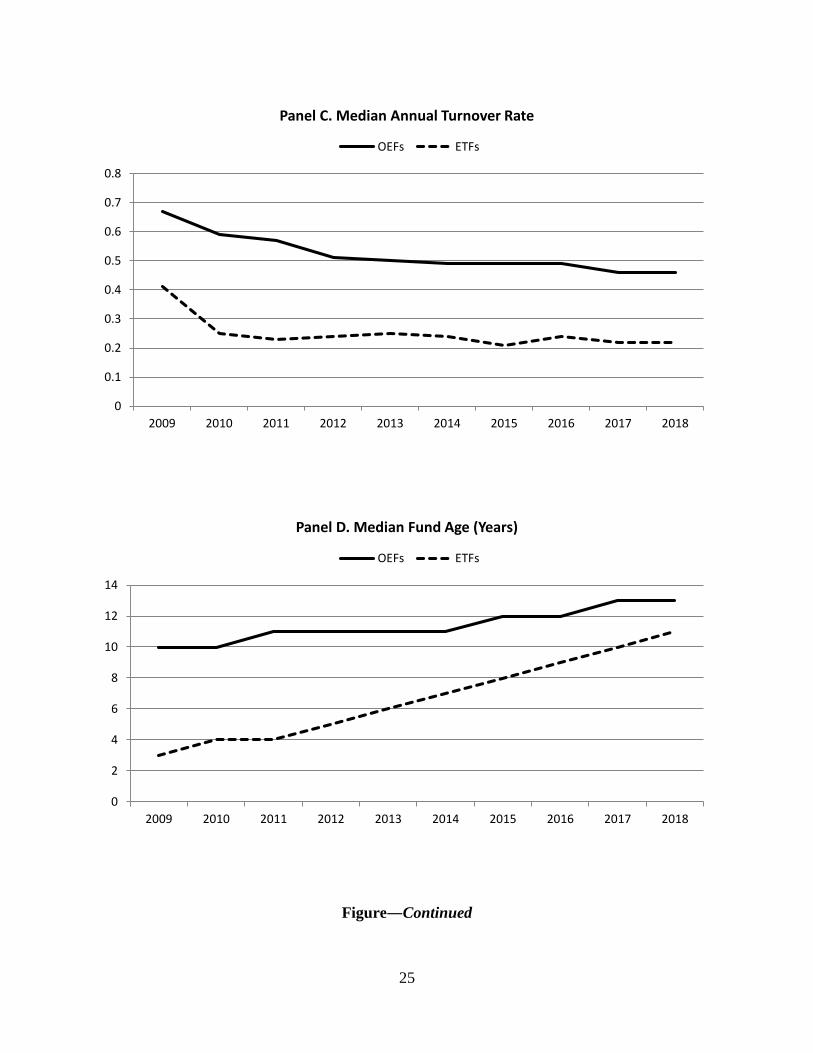
The Figure graphs the quarterly portfolios of all domestic actively managed OEFs and

passively managed equity ETFs in the CRSP database. Although the median OEF was about

$100 million higher in TNA than the median ETF in the early years, the median ETF rose above

the OEF TNA in 2018. The median OEF charges about twice the expense ratios and has double

the turnover rates than its counterpart ETF. While the median OEF was about six years older

than the median ETF in the early years, the age gap is about two years now.

III. ETF Investment by OEFs

Investing in an exchange-traded fund (ETF), which typically tracks a certain index, is costly for

an open-end equity fund (OEF) because the mutual fund can invest directly in the underlying

securities without paying management fees to the ETF. Nor are professional money managers

likely unaware of the dark side of ETF investment that studies document. How often do actively

managed open-end domestic equity funds invest in passively managed domestic equity ETFs?

Panel A of Table 1 shows that on average OEFs that invest in ETFs account for 14% of

the OEF population, while OEFs that do not invest in ETFs account for 86%. In total, U.S. OEFs

manage about $4.52 trillion assets, and those that invest in ETFs account for 9% of the total

assets. OEFs that do not invest in any ETFs hold fewer securities in their portfolios, and are

9 To mitigate the incubation bias, Cici, Gibson, and Moussawi (2010) and Kacperczyk, Sialm, and Zheng (2008)

exclude funds with assets of less than $5 million in the previous month. This filter might unintentionally exclude

Ameritor Security Trust (crsp_fundno: 005371; Ticker: ASTRX) from the calculations in January-May 1996

because its TNA was below $5 million in the previous months, although it was a seasoned fund. Its inception date

was December 1939, and its initial TNA $49 million was first recorded in December 1961.

7

much larger—they manage about $104 million more than their peers that invest in at least one

ETF in the median comparison.

Panel B shows that 28% of OEFs that invest in ETFs short a security, while 18% of OEFs

that do not invest in ETFs short a security. A similar number in terms of percentages of total

assets under management (%AUM) is also shown in Panel B. The difference is statistically

significant in both fraction and %AUM.

Panel C shows that the majority of OEFs that invest in ETFs take a long position in ETFs.

About 13% of OEFs that invest in ETFs short ETFs, and they also hold more securities in their

portfolio.

Panel D reports differences in attributes of total assets under management, expense ratios,

turnover rates, and fund ages of OEFs that invest in at least one ETF versus OEFs that do not.

OEFs that invest in ETFs are typically younger; they manage less assets, and they trade more

actively. OEFs that invest in ETFs could possibly pass the higher cost of ETF investment on to

shareholders by charging higher fees in the early years of the sample period, but that has become

much more difficult recently because of stiff competition in the mutual fund industry.

Furthermore, the median annual turnover rate varies from about 73% for OEFs that invest in

ETFs to about 49% for OEFs that do not invest in ETFs.

Table 2 classifies OEFs by Lipper classification codes. The result clearly shows that

OEFs invest in ETFs have a substantial presence in small-cap core and small-cap value funds (in

terms of both observations and net assets). Since small-cap stocks are more volatile and could be

hard to trade, an index-based ETF gives equity funds that invest primarily in small-cap stocks an

effective financial instrument for managing their portfolios. 10

As holding passive ETFs instead of the underlying securities directly is costly for mutual

funds, the reason might be for hedging. A passive ETF gives mutual funds a convenient and

liquid financial instrument to hedge against adverse movements in the broad stock market or a

market sector. A mutual fund that shorts individual stocks is also likely to take a long position in

10 In each quarter, domestic equity funds are classified into fourteen fund groups according to Lipper classification

codes (CRSP variable: lipper_class): LCCE (Large-Cap Core), LCGE (Large-Cap Growth), LCVE (Large-Cap

Value), MCCE (Mid-Cap Core), MCGE (Mid-Cap Growth), MCVE (Mid-Cap Value), SCCE (Small-Cap Core),

SCGE (Small-Cap Growth), SCVE (Small-Cap Value), MLCE (Multi-Cap Core), MLGE (Multi-Cap Growth),

MLVE (Multi-Cap Value), MAT+MT (Mixed-Asset Target-Date and Target-Allocation), and Other. The percentage

of fund observations in each group is of the total number of all funds each quarter. Total fund net asset value is also

calculated within each group and expressed relative to the total net assets of all funds each quarter.

8

ETFs for hedging. As a result, the hedging hypothesis predicts that mutual funds with positions

in ETFs tend to short securities.

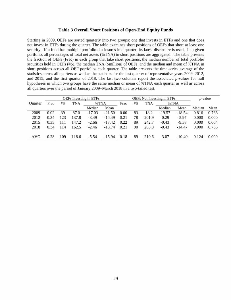
Table 3 reports the aggregate percentage of total net assets (%TNA) in all short positions

in a given OEF portfolio.11 OEFs that invest in ETFs tend to take short positions in a stock.

Table 3 clearly shows that on average 28% of all OEFs that invest in ETFs take short positions,

while about 18% of all OEFs that do not invest in ETFs take short positions. In the fourth quarter

of 2015, for example, 35% of OEFs that invested in ETFs shorted at least one security while 22%

of OEFs that did not invest in ETFs shorted at least one security.

Furthermore, in terms of the median (mean), the total percentage in all short positions in

a given portfolio held by OEFs that invest in ETFs is about two (one and a half) times that of

OEFs that do not invest in ETFs. For example, in the last quarter of 2015, the median overall

short position represents 2.66% of TNA among the OEFs that invest in ETFs compared to 0.43%

of TNA among the OEFs that do not invest in ETFs. The tendency of OEFs that invest in ETFs

to take short positions is significant, and consistent with the hedging hypothesis. This tendency,

together with the fact that OEFs that invest in an ETF and short at least one security have lower

total assets under management, seems to indicate that smaller equity funds use the index basket

provided by the ETF to engage in tactical behavior such as shorting.

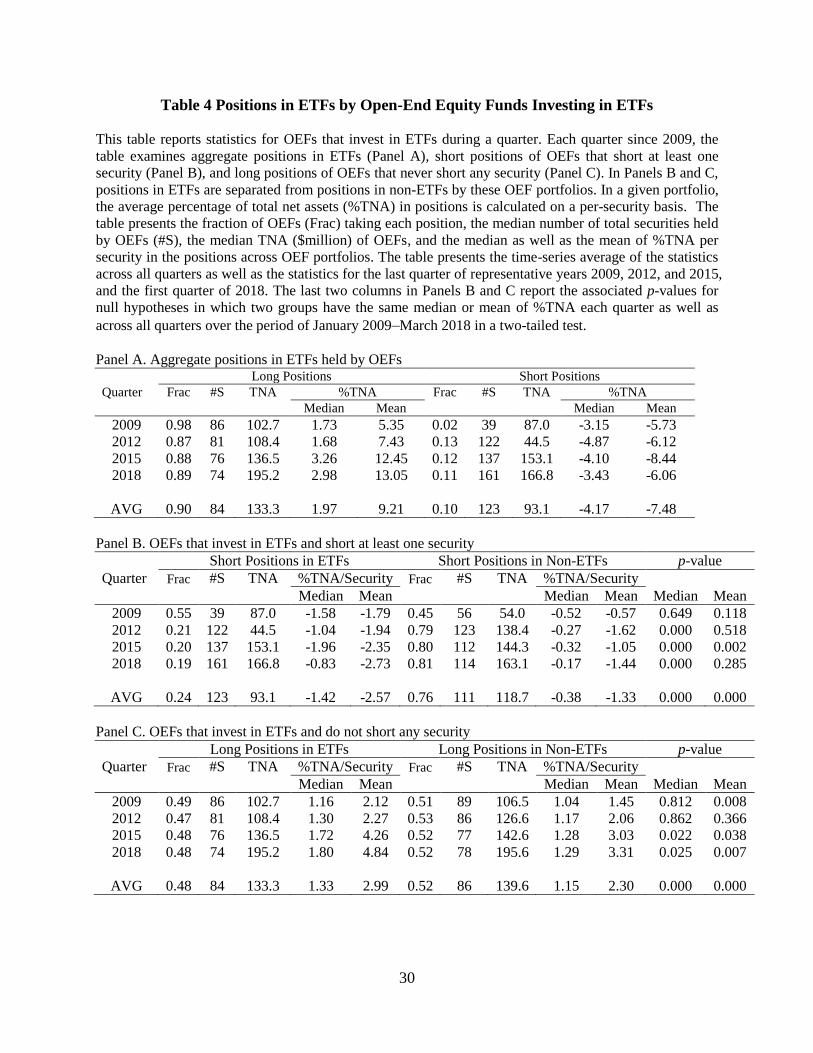
OEFs might also likely engage in active management by shorting individual stocks and

using ETFs as an investment base. Panel A of Table 4 shows that more OEFs take a long but

small position in ETFs, while fewer OEFs take a short but relatively large position in ETFs.

Since 2010, the median aggregate long position in ETFs has ranged from 1.34% in 2014Q2 to

3.26% in 2015Q4 of TNA in a given OEF portfolio; the median aggregate short position in ETFs

has ranged from 2.49% in 2016Q4 to 6.39% in 2015Q2.

To further investigate individual short positions held by OEFs that invest in ETFs, I

separate their short positions in ETFs from short positions in non-ETF securities. In a given

portfolio, I calculate the average percentage of total net assets (%TNA) in short positions on a

per-security basis. The results in Panel B indicate that OEFs that invest in ETFs short ETFs more

11 It is clear that the quality of the data on short positions in mutual fund holdings prior to 2010 Q2 is questionable. I

verified this observation with CRSP. The mutual fund holdings database (S12) from Thomson Reuters does not give

short portfolio holdings and has a limited set of securities other than US equities. Chen, Desai, and Krishnamurthy

(2013) cite the same reason for using the CRSP mutual fund database to examine short positions taken by mutual

funds. They study portfolio holdings of mutual funds that had outstanding short positions in US common stocks

from April 2003 through December 2006.

9

than other securities when they decide to take a short position. For example, in the fourth quarter

of 2015, their median short position in an ETF is 1.96% compared to the median short position in

any non-ETF security of 0.32%.

This evidence, which is strongly significant for both median and mean tests, seems to

support the assertion that OEFs short ETFs in order to protect their portfolios from negative

market shocks. Note the evidence in Panel C that OEFs that invest in ETFs and never short any

security, by comparison, have a similar long position in both ETFs and non-ETF securities.

IV. Tests of Three Competing Hypotheses

Besides using exchange-traded funds (ETFs) to hedge against adverse market movements, open-

end equity funds (OEFs) might use them as a liquid financial vehicle to gain exposure to hard-to-

trade assets or to manage hot fund flows. To differentiate the three competing hypotheses, I

investigate how OEF holdings deviate from ETF holdings, and examine how the degree of

portfolio overlap between the two determines subsequent changes in the ETF positions that

OEFs hold.

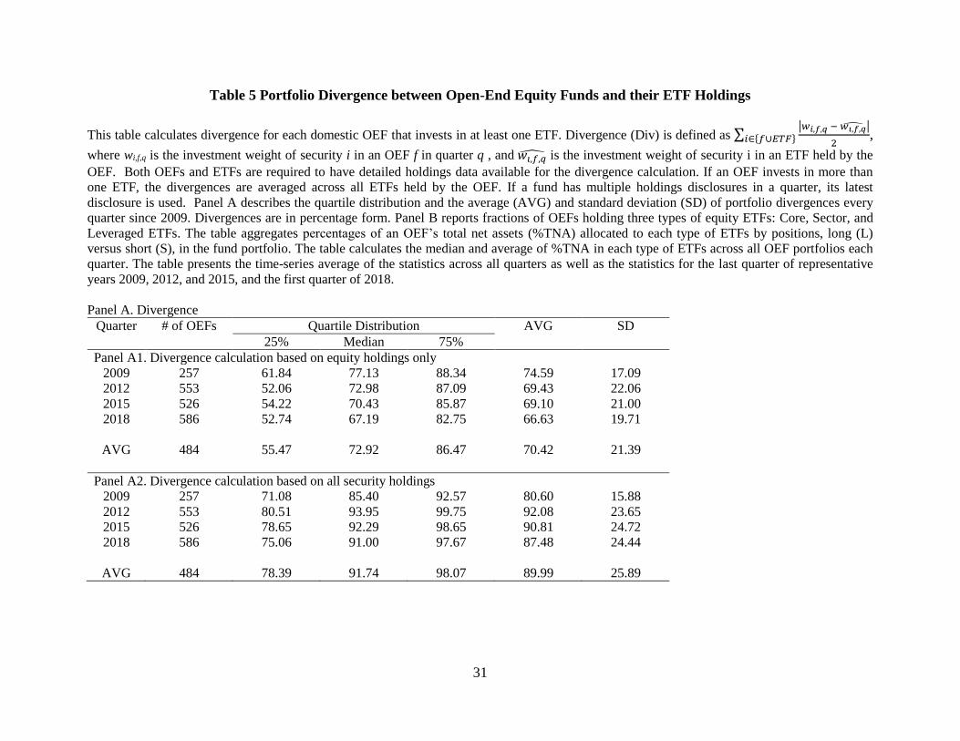
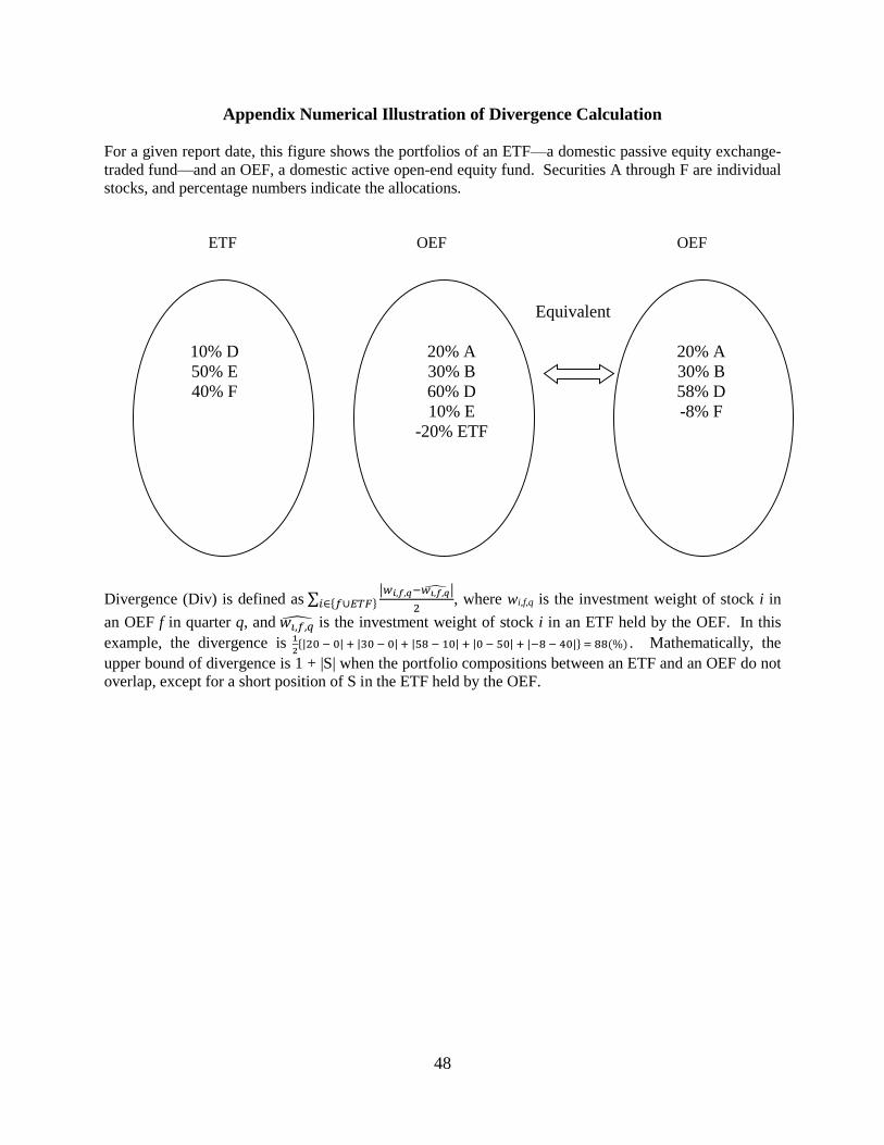
I follow the construction of “divergence” defined by Cheng, Massa, and Zhang (2013) to

quantify the overlap between OEF portfolios and ETF portfolios. Divergence (Div) is defined as

∑|𝑤𝑖,𝑓,𝑞 − 𝑤𝑖,𝑓,�̂�|

2𝑖∈{𝑓∪𝐸𝑇𝐹} , where wi,f,q is the investment weight of security i in OEF f in quarter q ,

and 𝑤𝑖,𝑓,�̂� is the investment weight of security i in an ETF held by the OEF. Both OEFs and

ETFs are required to have detailed holdings data in order to calculate divergence. 12

I calculate divergence for each domestic active OEF that invests in at least one domestic

passive ETF. If an OEF invests in more than one ETF, I calculate the divergence for each ETF it

holds, and average the divergences across all ETFs held. A numerical illustration of divergence

calculation is in the appendix.

If a fund issues multiple holdings disclosures in a quarter, I use its last disclosure for the

quarter. OEFs and ETFs held by the OEFs may not disclose portfolio holdings at the same time,

and most of the time they do not. To make divergence calculations as complete as possible, I use

the latest disclosed portfolio holdings of ETFs held by OEFs in the six months before the OEFs

12 The construction of “divergence” follows that of “active share” defined by Cremers and Petajisto (2009), except

that they calculate the difference in portfolio weights between an OEF and its benchmark.

10

disclose their ETF investment. As mutual funds can invest in non-equity securities such as bonds,

return swaps, or derivatives, I construct two divergence measures, one for equities only and the

other including all holdings.13

Table 5 presents the quartile distribution and the average and standard deviations of

portfolio divergences every quarter since 2009. The quartile distribution of divergences seems

relatively stable over time. In Panel A, when the divergence is calculated for equities (all

securities) held by mutual funds, the time-series average of median portfolio divergences

between OEFs and ETFs is 72.92% (91.74%).

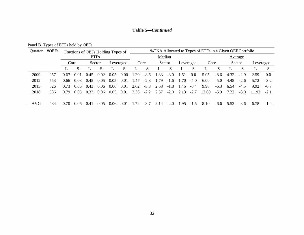
In Panel B, to further understand the types of ETFs that OEFs commonly hold, I classify

equity ETF holdings into three types, Core ETFs, Sector ETFs, and Leveraged ETFs.14 I separate

long positions from short positions in ETFs held by OEFs. The majority of OEFs that invest in

ETFs, about 70%, take a long position in Core ETFs. Among these OEFs, the median

(average) %TNA allocated to Core ETFs is 1.72% (8.1%) in a given portfolio. About 41% of

OEFs that invest in ETFs take a long position in Sector ETFs. Among these OEFs, the median

(average) %TNA allocated to Sector ETFs is 2.14% (5.53%) in a given portfolio. Some OEFs

may invest in multiple types of ETFs, and few OEFs hold leveraged ETFs in their portfolios.

To clarify the main motivation of OEF investment in ETFs, Table 6 reports the degree of

overlap in portfolio holdings between OEFs and the ETFs that they hold, and of subsequent

changes in ETF positions by these OEFs. Each quarter, I sort OEFs into quartiles according to

their divergence. For each OEF in each quarter, I aggregate all %TNA allocated to ETFs in long

and short positions separately, and calculate changes in ETF positions from the portfolio-

formation quarter to the next quarter.

OEFs in the extreme quartiles are the sample funds most involved in differentiating the

hedging hypothesis from the substitution hypothesis. The hedging hypothesis clearly predicts

that OEFs whose portfolio composition most overlaps with a target ETF will increase short

13 In the CRSP Mutual Fund Database, I use “permno” to identify equities and “crsp_company_key” to identify non-

equity securities. Foreign stocks or non-security instruments held by mutual funds are also assigned by

“crsp_company_key.” According to the CRSP website, crsp_company_keys should match up one to one with

portfolio holdings and not be reused. 14 Core ETFs are domestic U.S. equity ETFs excluding all Sector and Leveraged ETFs. Sector ETFs have “EDS” in

the first three characters of the CRSP Style Code (variable: crsp_obj_cd), while Leveraged ETFs have “EDYH” or

“EDYS” in their style codes. According to CRSP, funds with a style code of “EDYH” include long/short equity

funds, equity market neutral funds, absolute return funds, and equity leverage funds. Funds with a style code of

“EDYS” include dedicated short biased funds.

11

positions and reduce long positions in the target ETF subsequently. Indeed, OEFs in quartile 1

behave as the hedging hypothesis predicts. The substitution hypothesis predicts that OEFs in

quartile 4 will increase long positions in ETFs, but the result shows instead that these OEFs

reduce long positions on ETFs significantly. According to the substitution hypothesis, concern

with regard to restrictions on illiquid assets would motivate an OEF to invest in a liquid ETF

instead of its hard-to-trade underlying assets. In this case, there is very little overlap in portfolio

composition between the OEF and the ETF that it holds.

Managers may be reluctant to invest in or actually divest securities immediately if the

timing of cash flows does not correspond to managers’ view of optimal trading. In a model

describing mutual fund managers that satisfy the liquidity needs of their clients as discretionary

liquidity traders, Subrahmanyam (1991) shows that fund managers would trade a basket instead

of individual securities in order to minimize adverse selection costs. Edelen (1999) shows that

mutual fund trades that are related to cash flows are less profitable than trades that are not so

influenced by cash inflows. ETFs may let a fund manager maintain a desired exposure to the

market or to certain sectors while waiting for more information on which to execute individual

stock trades; this might allow for more efficient management of considerable money to and from

a fund. The flow management hypothesis predicts that mutual funds tend to increase positions in

ETFs right after a surge of fund inflows and to reduce positions after a persistent outflow. I argue,

however, that large firms in an industry may give fund managers an investment opportunity,

without paying ETFs management fees, to obtain a similar exposure.

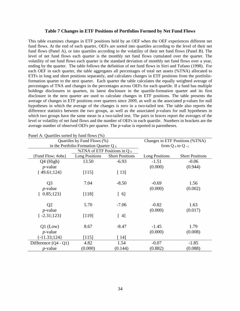
Table 7 examines changes in an OEF’s ETF positions when the OEF experiences

different net fund flows. At the end of each quarter, I sort OEFs into quartiles according to the

level of their net fund flows in Panel A and according to the volatility of their net fund flows in

Panel B. The level each quarter is the monthly net fund flows cumulated over the quarter. The

volatility of net fund flows each quarter is the standard deviation of monthly net fund flows over

the prior year. I use the definition of net fund flows in Sirri and Tufano (1998). For each OEF in

each quarter, I aggregate all %TNA allocated to ETFs in long and short positions separately and

calculate changes in ETF positions from the portfolio-formation quarter to the next quarter.

In Panel A of Table 7, although OEFs that experience surging fund inflows in the current

quarter have overall larger long positions in ETFs (about 4.82% higher) and smaller short

positions (about 1.54% lower) than the positions held by OEFs that experience fund outflows,

12

OEFs in Q4 reduce their long positions but increase short ones in ETFs in the next quarter. When

quartiles are formed according to the volatility of net fund flows in Panel B of Table 7, OEFs

that experience volatile fund flows significantly reduce long positions in ETFs much more in the

next quarter than OEFs that experience stable fund flows.

Overall, Table 7 does not support the assertion of the flow management hypothesis that

fund inflows and outflows prompt OEFs to change their ETF holdings. If there is any indication

that OEFs use ETFs to manage fund flows, we see this in the evidence that OEFs significantly

reduce both long and short positions in ETFs after volatile fund flows.

V. Tests on Performance and Risk of ETF Investment

To further investigate the motivation for an open-end equity fund (OEF) to invest in exchange-

traded funds (ETFs), I examine the performance and risk of OEFs before and after their ETF

investment. For each domestic actively managed OEF, I identify the first month-end (t0) and the

last month-end (t1) in which the OEF invested in domestic passively managed equity ETFs. I

examine the performance and risk of OEFs over three periods: the pre-holding period (Pre-H) of

[t0−36, t0], the holding period (H) of [t0, t1], and the post-holding period (Post-H) of [t1, March

2018]. To eliminate temporary holdings in ETFs, I analyze only OEFs that held ETFs in their

portfolios for at least a year. I use OEF monthly gross returns to estimate the alpha of the Fama-

French (1996) three factors plus a momentum factor for each fund portfolio in each period, and

calculate the fund’s information ratio, the alpha divided by the standard deviation of the four-

factor residuals. In each period, an OEF must have at least 12 monthly returns in order to

estimate its four-factor alpha and to test the null hypothesis that the average of information ratios

is equal to zero in a two-tailed test.

Panel A of Table 8 shows that OEFs cannot enhance the four-factor information ratios

simply by investing in passive ETFs. For example, the four-factor information ratio of OEFs is

−0.077% per month over the holding period, which represents a 0.061% decline per month from

the pre-holding period to the holding period. The average length of the holding periods across all

OEFs investing in ETFs is 56 months; the average length of the pre-holding periods is about 32

months. That the holding period is longer than four years seems to indicate that OEFs use ETFs

systematically for portfolio management, instead of just occasional investment.

13

Although most of the parametric tests on the four-factor information ratios are

significantly negative in Panel A, the results may not be robust when the underlying data exhibit

unknown forms of conditional and unconditional heteroscedasticity. In a robustness check, I

present statistics based on a bootstrap simulation. The simulation design follows that of Fama

and French (2010). A simulation run is a random sample (with replacement) of 111 months,

drawn from the 111 calendar months of January 2009 through March 2018. I estimate, fund by

fund, the four-factor alpha on the simulation draw of months of fund gross returns, eliminating

funds that are in the simulation run for under 12 months. Each run thus produces cross-sections

of information ratio estimates using the same random sample of months from populations of

OEFs that invest in an ETF.

Fama and French (2010) document that such a simulation approach can capture the cross-

correlation of fund returns and its effects on the distribution of alpha estimates. Furthermore, it

also captures any correlated heteroscedasticity of the explanatory returns and disturbances of a

factor model, because the approach jointly samples fund and explanatory returns. I present the

percentage of 10,000 simulation runs that produce the average of cross-sectional information

ratios below the actual four-factor average in the third line of Panel A. For example, the average

four-factor information ratio of −0.077% over holding period H in which the OEFs invested in

ETFs exceeds the simulated fund return cross-sectional average in 4,693 of 10,000 simulation

runs, as indicated by 46.93% in brackets.15

Panel B reports the statistics for OEFs with high divergence (86% above) and OEFs with

low divergence (55% and below), where the divergence is calculated on the basis of equity

holdings only. These divergences closely correspond to the 75th and 25th percentiles of

divergence distribution in Table 5. Compared to OEFs that exhibit low divergence with ETFs,

OEFs that exhibit higher divergence show a better (but insignificant) information ratio, 0.012%

per month over the holding period.

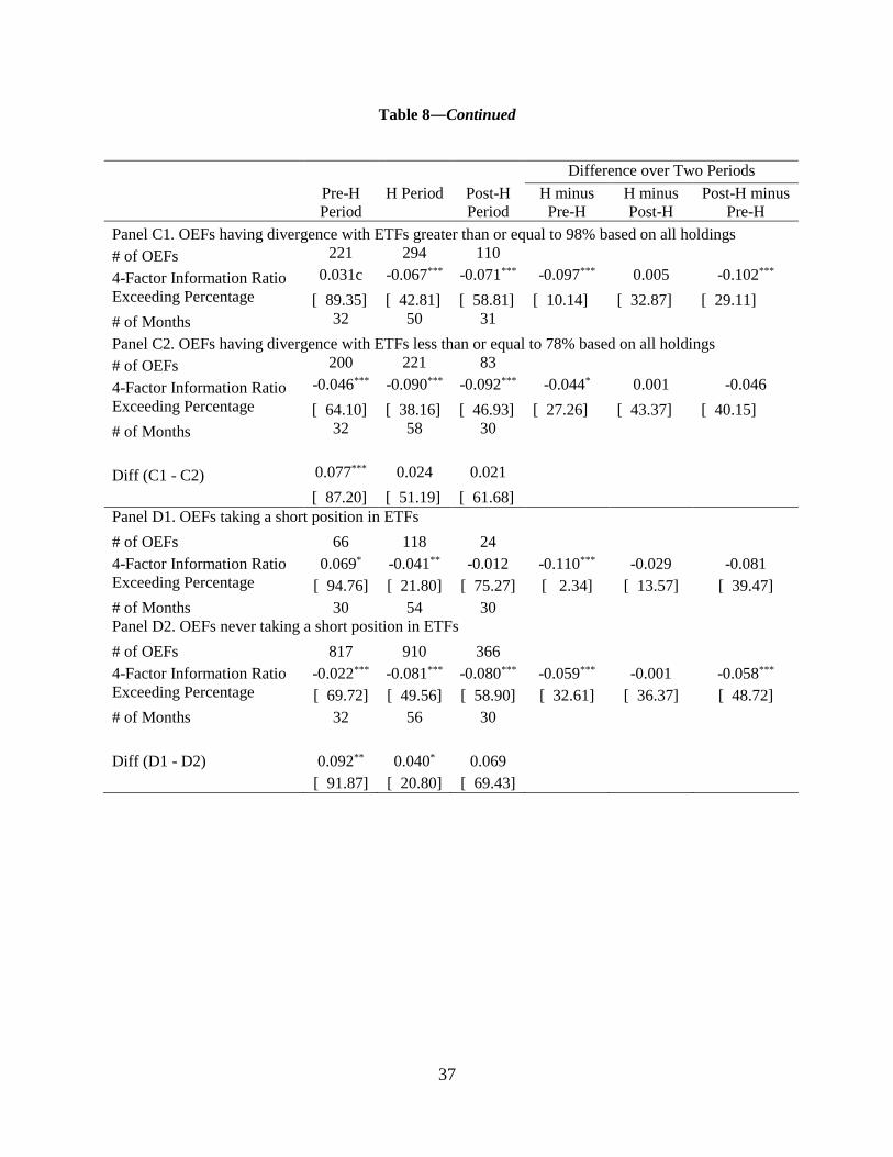
When the divergence is calculated for all holdings, the corresponding 75th and 25th

percentiles of divergence distribution are at 98% and 78%, respectively, as displayed in Panel C.

Compared to OEFs that exhibit low divergence with ETFs, OEFs that exhibit higher divergence

show a better (but insignificant) information ratio, 0.024% per month over the holding period.

15 In a robustness check of the simulation, I jointly sample fund and explanatory returns as well as the month a fund

begins and ends a position in an ETF. The results are similar (available upon request).

14

Panel D reports the statistics for OEFs that take at least a short position in ETFs and

OEFs that never take a short position in any ETF during the holding period. While Panels B and

C show that OEFs that engage in passive ETF investment cannot improve their performance,

Panel D shows that OEFs that short ETFs have significantly higher information ratios than OEFs

that do not short ETFs in both pre-holding and holding periods. The result holds when the four-

factor alphas are estimated on net-of-expense returns.

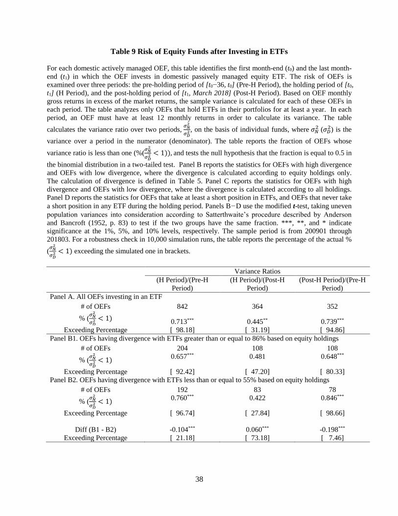
One reason an OEF might use ETFs is to hedge against adverse market moves or to

participate in the broad movement of the stock market and thus potentially reduce overall

portfolio volatility. To quantify the reduction in active risk, Table 9 examines the risk of OEFs

relative to the market after they invest in ETFs. Panel A shows that, overall, 71.3% of OEFs that

invest in ETFs reduce the volatility of their returns in excess of market returns from the pre-

holding period to the holding period, and 73.9% of OEFs reduce their relative return volatility

from the pre-holding to the post-holding period. Both percentages of the variance ratio indicate

significant rejection of the null hypothesis (at the 1% level) that the fraction is equal to 0.5 in the

binomial distribution in a two-tailed test.16

In a robustness check using the bootstrap simulation proposed by Fama and French

(2010), in 9,818 of 10,000 simulation runs funds reduced their relative return volatility from the

pre-holding period to the holding period less than 0.713. Thus, it is not random that 71.3% of

OEFs investing in ETFs reduced the relative return volatility.

Once OEFs implement a risk-reduction strategy using ETFs, they seem to pursue it

constantly to manage risk in the post-holding period. It may be due to construction of the holding

period, which does not rule out that OEFs might hold ETFs on and off during the holding period,

that 44.5% of OEFs that invest in ETFs have low relative return volatility in the holding period

over the post-holding period. Also, there are many fewer OEFs with at least 12 monthly returns

in the post-holding period, which might diminish the reliability of comparisons for the post-

holding period.

Panels B through D further examine the risk reduction of OEFs relative to high or low

divergence with ETFs as well as short or long positions in ETFs. These results support a similar

16 In a related study, Koski and Pontiff (1999) document that the difference in performance as measured by alpha

between funds that use derivatives and those that do not is insignificant, but fund managers might be using

derivatives to reduce the impact of prior performance on risk taking. When I extend the analysis using 60 months

instead of 36 months as the pre-holding period, I obtain a similar result.

15

conclusion as in Panel A. Additionally, a significantly higher percentage of OEFs reduce return

volatility from the pre-holding to the holding period with regard to low divergence with ETFs

than high divergence with ETFs.

There is no way an equity fund can improve its performance simply by holding ETFs. At

the aggregate level, can OEFs investing in ETFs perform better than OEFs not investing in ETFs,

given that index-based ETFs provide a convenient and liquid financial instrument for mutual

funds? To investigate this issue, each quarter I classify OEFs into two portfolios: one that

includes funds that invest in ETFs, and one that includes funds that do not invest in any ETF. I

calculate the value-weighted gross returns of these two portfolios over three months following

portfolio formation, using as a weight the TNA value of a fund at the beginning of each month.

At the end of the sample period, I regress monthly excess returns of each portfolio on the Fama-

French three factors plus a momentum factor.

Panel A of Table 10 shows that the four-factor alphas of these two portfolios cannot be

differentiated. This finding further confirms that OEFs as a whole cannot perform better by

including ETFs in their portfolio strategies.

While OEFs short ETFs for hedging against adverse market movements, they might also

take a long position in ETFs to gain quick market exposure and benefit from the active stock

selection. This would require that the OEFs allocate a significant position to stocks outside the

ETF basket to gain meaningful performance improvement over the ETF.

Panel B of Table 10 clearly shows that OEFs taking a long position only in ETFs are

greatly exposed to the market (RMRF) and the small-minus-big (SMB) factor, but this results in

a significantly negative four-factor alpha. OEFs shorting ETFs indeed outperform OEFs taking

long positions in ETFs by 15.1 basis points per month, although the difference is insignificant.

Given that OEFs shorting ETFs are exposed much less to RMRF and more negatively to

momentum (MOM), this indicates that OEFs short ETFs to hedge against adverse movement of

the stock market.

VI. Multivariate Analyses

So far, I have explored several variables that might individually explain why active open-end

equity funds (OEFs) take positions in passive exchange-traded funds (ETFs). Yet these variables

are not mutually exclusive, and some might be more important than others. The variables might

16

moreover have different explanatory power under different market conditions. Accordingly, I

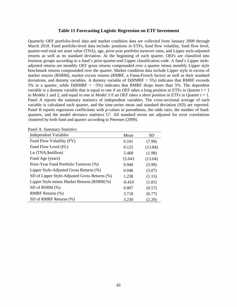
examine the variables simultaneously in a forecasting logistic panel regression.

Although we cannot know ex-ante what triggers an OEF to invest in an ETF, I make

several attempts in forecasting logistic panel regressions in the hope of understanding the reason.

First, I link fund flows, performance, risk, and characteristics of OEFs as well as market

conditions to the ETF investment decision. The forecasting logistic panel regression is:

𝑌𝑖,𝑡+1 = 𝛼 + 𝛽1𝐹𝑙𝑜𝑤𝑖,𝑡 + 𝛽2𝑃𝑒𝑟𝑓𝑜𝑟𝑚𝑎𝑛𝑐𝑒𝑖,𝑡 + 𝛽3𝑅𝑖𝑠𝑘𝑖,𝑡 + 𝐶𝑜𝑛𝑡𝑟𝑜𝑙𝑠 + 𝜀𝑖,𝑡+1 (1)

where Yi,t+1 is a binary variable for Fund i in Quarter t+1.

In Models 1 and 2 of Table 11, the dependent variable takes a value of one if an OEF

takes a long position in ETFs in Quarter t+1; in Model 3 the dependent variable takes a value of

one if an OEF takes a short position in ETFs in Quarter t+1. Flowi,t is the lagged net fund flow

measure for i. The level (volatility) of net fund flows each quarter is the sum (standard deviation)

of monthly net fund flows over the quarter. A fund’s performance is measured by the difference

in returns between the fund and its style benchmark. At the beginning of each quarter, OEFs are

sorted into 14 groups according to the fund’s prior-quarter-end Lipper classification code defined

in Table 2, and the value-weighted Lipper style benchmark returns are calculated each month

using a fund’s TNA at the beginning of each month as a weight. Quarterly cumulative abnormal

returns are monthly OEF gross returns compounded over a quarter minus monthly Lipper style

benchmark returns compounded over the quarter. A fund’s risk is measured by the standard

deviation of monthly abnormal returns.

The controls in Quarter t include quarter-end fund total net asset value (TNA), fund age,

prior-year fund portfolio turnover rate, a fund’s style returns in excess of the market returns

(RSRM), the standard deviation of monthly RSRM, cumulative market excess return (RMRF, a

Fama-French factor), the standard deviation of monthly RMRF, and dummy variables. Monthly

RSRM are returns on a fund’s Lipper style benchmark minus returns on the market, the value-

weighted CRSP stock index. Quarterly cumulative RSRM and RMRF are calculated in a way

similar to calculation of the fund’s cumulative abnormal returns. A dummy variable of

D(RMRF>5%) indicates that RMRF exceeds 5% in a quarter while D(RMRF< −5%) indicates

17

that RMRF drops more than 5% in a quarter. 17 All standard errors are adjusted for error

correlations clustered by fund and quarter according to Petersen (2009).

Table 11 shows OEFs that experienced fund outflows, underperformed their style

benchmark, or showed less volatility of tracking errors will likely take a long position in ETFs

next quarter, particularly following a quarter when the OEFs’ Lipper style benchmark

underperformed the stock market. That mutual funds would take a long position in ETFs after an

exodus of fund flows is contrary to the prediction of the flow management hypothesis.

Model 3 in Panel B of Table 11 shows OEFs that were newly established,

underperformed their style benchmark, or showed higher volatility of tracking errors will likely

take a short position in ETFs next quarter, particularly following a quarter when the OEFs’

Lipper style benchmark underperformed the stock market and their style benchmark was more

volatile than the stock market. Furthermore, OEFs will likely take a short position in ETFs

following a quarter when the stock market underperformed the T-bill and the stock market was

not very volatile, but OEFs are unlikely to take a short position in ETFs following a quarter of

severe market downturn, for example, when the RMRF drops more than 5%.

One caveat for this interpretation, particularly in examining OEFs’ short positions in

ETFs: OEFs that do not invest in ETFs account for 86% of the OEF population, and only 13% of

OEFs that do invest in ETFs short them. The fund-quarter observations in the regressions are

dominated by OEFs that do not invest in ETFs. As a result, the fact that very few OEFs short

ETFs makes parameter estimates unconverged when we include the fund flow level in the

explanatory variables.

An OEF not intending to invest in an ETF or temporarily holding an ETF does not

provide much information about why OEFs in general invest in ETFs. Therefore, I next focus on

OEFs that owned ETFs in prior quarters, and examine their strategies with respect to their ETF

holdings. By gaining information on how an OEF takes positions in ETFs in response to changes

in fund flows, the degree of composition overlap between the OEF and its ETF holdings, and

extreme market conditions in a logistic panel regression, we might be able to differentiate the

three hypotheses. The forecasting logistic panel regression is:

17 In a robustness check, an extreme market with a big swing is defined using the cut-off return of 2% for RMRF in

a quarter. The result is similar, except for the significance of coefficients associated with RMRF (available upon

request).

18

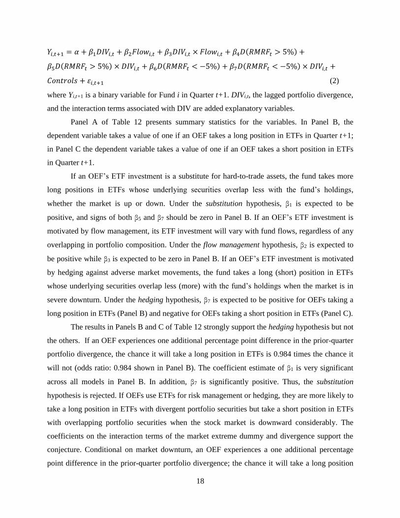
𝑌𝑖,𝑡+1 = 𝛼 + 𝛽1𝐷𝐼𝑉𝑖,𝑡 + 𝛽2𝐹𝑙𝑜𝑤𝑖,𝑡 + 𝛽3𝐷𝐼𝑉𝑖,𝑡 × 𝐹𝑙𝑜𝑤𝑖,𝑡 + 𝛽4𝐷(𝑅𝑀𝑅𝐹𝑡 > 5%) +

𝛽5𝐷(𝑅𝑀𝑅𝐹𝑡 > 5%) × 𝐷𝐼𝑉𝑖,𝑡 + 𝛽6𝐷(𝑅𝑀𝑅𝐹𝑡 < −5%) + 𝛽7𝐷(𝑅𝑀𝑅𝐹𝑡 < −5%) × 𝐷𝐼𝑉𝑖,𝑡 +

𝐶𝑜𝑛𝑡𝑟𝑜𝑙𝑠 + 𝜀𝑖,𝑡+1 (2)

where Yi,t+1 is a binary variable for Fund i in Quarter t+1. DIVi,t, the lagged portfolio divergence,

and the interaction terms associated with DIV are added explanatory variables.

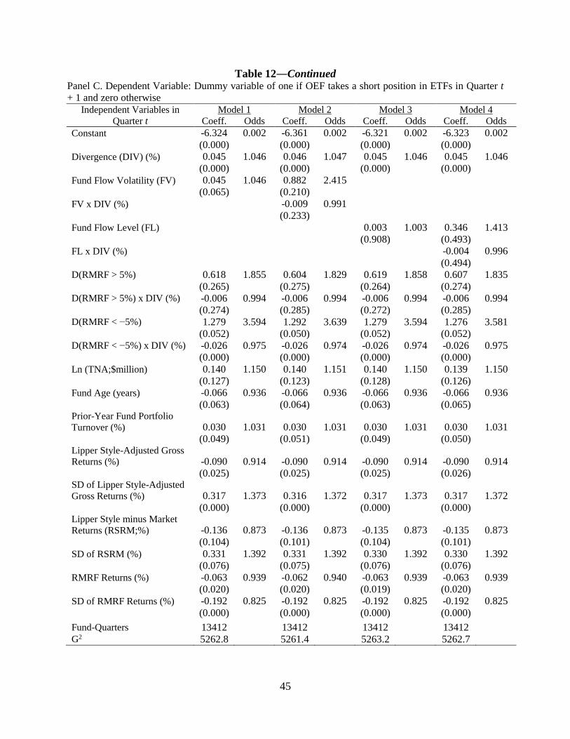
Panel A of Table 12 presents summary statistics for the variables. In Panel B, the

dependent variable takes a value of one if an OEF takes a long position in ETFs in Quarter t+1;

in Panel C the dependent variable takes a value of one if an OEF takes a short position in ETFs

in Quarter t+1.

If an OEF’s ETF investment is a substitute for hard-to-trade assets, the fund takes more

long positions in ETFs whose underlying securities overlap less with the fund’s holdings,

whether the market is up or down. Under the substitution hypothesis, β1 is expected to be

positive, and signs of both β5 and β7 should be zero in Panel B. If an OEF’s ETF investment is

motivated by flow management, its ETF investment will vary with fund flows, regardless of any

overlapping in portfolio composition. Under the flow management hypothesis, β2 is expected to

be positive while β3 is expected to be zero in Panel B. If an OEF’s ETF investment is motivated

by hedging against adverse market movements, the fund takes a long (short) position in ETFs

whose underlying securities overlap less (more) with the fund’s holdings when the market is in

severe downturn. Under the hedging hypothesis, β7 is expected to be positive for OEFs taking a

long position in ETFs (Panel B) and negative for OEFs taking a short position in ETFs (Panel C).

The results in Panels B and C of Table 12 strongly support the hedging hypothesis but not

the others. If an OEF experiences one additional percentage point difference in the prior-quarter

portfolio divergence, the chance it will take a long position in ETFs is 0.984 times the chance it

will not (odds ratio: 0.984 shown in Panel B). The coefficient estimate of β1 is very significant

across all models in Panel B. In addition, β7 is significantly positive. Thus, the substitution

hypothesis is rejected. If OEFs use ETFs for risk management or hedging, they are more likely to

take a long position in ETFs with divergent portfolio securities but take a short position in ETFs

with overlapping portfolio securities when the stock market is downward considerably. The

coefficients on the interaction terms of the market extreme dummy and divergence support the

conjecture. Conditional on market downturn, an OEF experiences a one additional percentage

point difference in the prior-quarter portfolio divergence; the chance it will take a long position

19

in ETFs is 1.010 times the chance it will not, and the chance it will take a short position in ETFs

is about 0.975 times the chance it will not. Thus, the hedging hypothesis is supported.

The coefficient estimates of fund flow volatility and level are insignificant. This implies

that fund flow management is not the main consideration for an OEF to take a position in ETFs.

When the interaction between the fund flow volatility and the portfolio divergence is considered

in Model 2, OEFs experiencing volatile fund flows are unlikely to take a long position in ETFs

as shown in Panel B.

An OEF experiencing higher portfolio turnover tends to take a short but not a long

position in ETFs. When OEFs have outperformed their style peers, they are likely to take a long

position in ETFs but unlikely to take a short position. OEFs tracking their style benchmark well

(i.e., experiencing low volatility of relative performance) are better able to engage in tactical

asset allocation using ETFs, so these OEFs are more likely to take a long but not a short position

in ETFs. When an OEF investment style has experienced more performance volatility than the

market, the OEF is unlikely to take a long position in ETFs but more likely to take a short

position. Shorting becomes more expensive in a volatile stock market, so OEFs aiming to hedge

are unlikely to take a short position in ETFs. Furthermore, when the market has underperformed

the Treasury bill, OEFs are more likely to take a short position in ETFs.

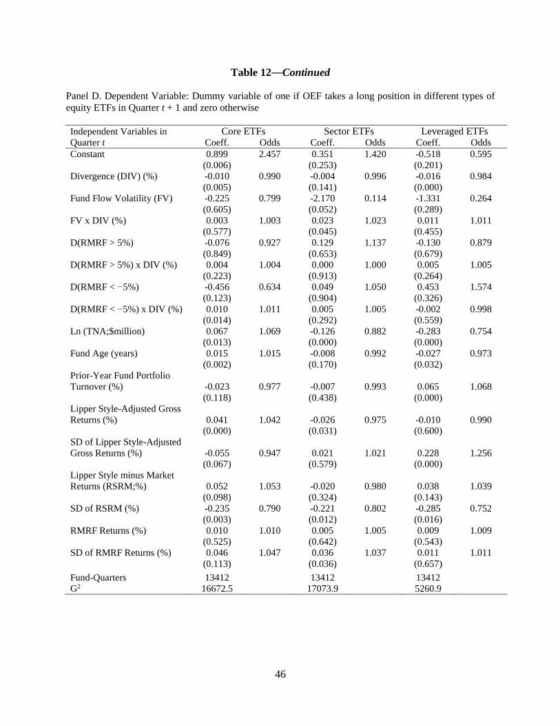
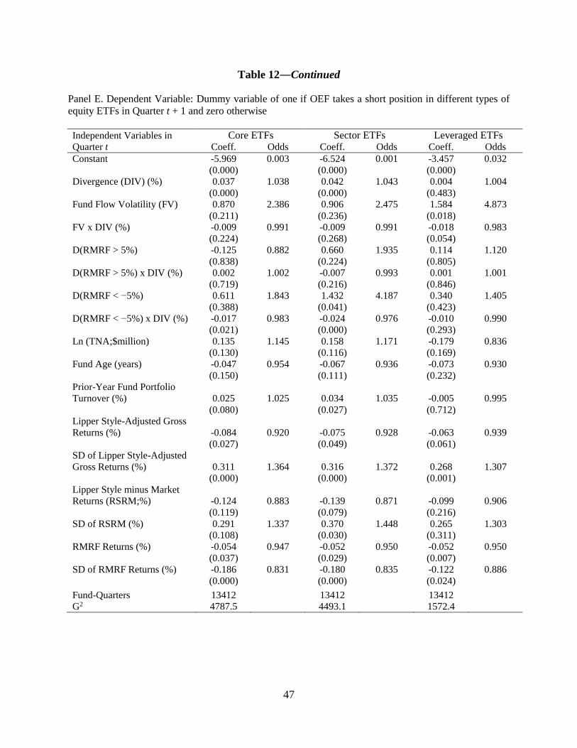
To understand whether this behavior applies only to a certain type of ETF, in Panels D

and E of Table 12 I further examine the types of ETFs in which OEFs are more likely to invest.

An advocate of the substitution hypothesis might argue that mutual funds most likely use sector

ETFs as a substitute for less liquid assets underlying the sector ETFs. Still, there is no evidence

for Sector ETFs shown in Panel D to support the substitution hypothesis. Nor is there evidence

supporting the flow management hypothesis across different types of ETF investment in Panels

D and E.

The hedging hypothesis, however, is supported in the case of Core ETF investment. Core

ETFs typically track a broad market index such as the S&P 500 Index. When the market is in

turmoil, OEFs are more likely to take a long position in a Core ETF with divergent portfolio

securities but take a short position in a Core ETF with overlapping portfolio securities.

Furthermore, shorting securities is very expensive, particularly in a bull or very volatile market.

Under such a scenario, OEFs are less likely to take a short position in any type of ETFs as shown

in the coefficients of RMRF and its standard deviation in Panel E.

20

VII. Conclusion

Given the transparency of the underlying assets in an exchange-traded fund, fees make it costly

for a mutual fund to hold an ETF rather than directly hold the underlying securities. Moreover,

an ETF investment by a mutual fund is surely open to criticism—why should fund shareholders

pay an extra fee when a mutual fund engages in passive ETF investment? Investors can simply

invest in passive ETFs by themselves. Why then do active mutual funds invest in passive ETFs?

First, this study shows that open-end equity funds (OEFs) that invest in ETFs tend to take

short positions in securities. They take about twice the number of short positions in general than

OEFs that do not invest in an ETF. This tendency to take a short position is very significant and

consistent with a hedging hypothesis. OEFs that invest in ETFs also short ETFs more than other

securities when they decide to take a short position. Furthermore, OEFs with overlapping

portfolio positions with a target ETF significantly reduce long positions and increase short

positions in the target ETF in subsequent investments. This piece of evidence seems to support

an assertion that OEFs short ETFs in order to protect their portfolios against negative market

shocks.

This study finds little evidence that OEFs change their ETF holdings in response to fund

inflows and outflows. If there is any evidence that OEFs use ETFs to manage fund flows, it is

that OEFs significantly reduce long positions in ETFs in response to volatile fund flows. Nor

does this study find evidence that liquid ETFs are a preferred venue for equity funds to invest in

hard-to-trade stocks that underlie the ETFs.

Although there is no way for equity funds to enhance the four-factor information ratios

simply by holding ETFs, they can reduce overall portfolio volatility significantly according to

results of both parametric tests and bootstrap simulations. While the funds that invest in ETFs

generally do not perform better, there is some evidence that OEFs that take short positions only

in ETFs outperform those that take long positions only in ETFs.

Finally, results of a multivariate logistic regression strongly support the hedging

hypothesis and not the substitution or the flow management hypotheses. The analysis also shows

that an OEF with more assets under management is unlikely to take long positions in ETFs. A

large established equity fund has enough assets to implement a dynamic investment strategy

using individual securities in order to maintain a desired exposure to the market, so ETF

investment is unnecessary.

21

OEFs that have underperformed their style benchmark, and have experienced higher

volatility of tracking errors, will likely take a short position in ETFs next quarter, particularly

following a quarter when their Lipper style benchmark underperformed the stock market and was

more volatile than the stock market. OEFs will likely take a short position in ETFs following a

quarter when the stock market underperformed the T-bill and the market was not very volatile.

OEFs not intending to invest in an ETF do not provide much information about why an

OEF invests in ETFs. It is instructive to focus on OEFs that have owned ETFs in prior quarters,

and examine how these OEFs pursue strategies shown in their ETF holdings. If an OEF’s ETF

investment is motivated by hedging against adverse market movements, the fund takes a long

(short) position in ETFs whose underlying securities overlap less (more) with its own holdings

when the market declines considerably. Results overall strongly support the hedging hypothesis,

and reject both the substitution hypothesis and the flow management hypothesis.

22

References

Anderson, Richard Loree, and Theodore Alfonso Bancroft, 1952, Statistical Theory in Research,

McGraw-Hill Book Company, New York.

Ben-David, Itzhak, Francesco A. Franzoni, and Rabih Moussawi, 2018, Do ETFs increase

volatility? Journal of Finance 73, 2471–2535.

Bhattacharya, Ayan, and Maureen O’Hara, 2017, Can ETFs increase market fragility? Effect of

information linkages in ETF markets, working paper, Cornell University.

Chen, Honghui, Hemang Desai, and Srinivasan Krishnamurthy, 2013, A first look at mutual

funds that use short sales, Journal of Financial and Quantitative Analysis 48, 761–787.

Cheng, Si, Massimo Massa, and Hong Zhang, 2013, The dark side of ETF investing: A world-

wide analysis, INSEAD working paper.

Cici, Gjergji, Scott Gibson, and Rabih Moussawi, 2010, Mutual fund performance when parent

firms simultaneously manage hedge funds, Journal of Financial Intermediation 19, 169–187.

Cremers, K. J. Martijn, and Antti Petajisto, 2009, How active is your fund manager? A new

measure that predicts performance, Review of Financial Studies 22, 3329–3365.

Da, Zhi, and Sophie Shive, 2018, Exchange traded funds and asset return correlations, European

Financial Management 24, 136–168.

Edelen, Roger, 1999, Investor flows and the assessed performance of open-end fund managers,

Journal of Financial Economics 53, 439–466.

Elton, Edwin J., Martin J. Gruber, and Christopher R. Blake, 2001, A first look at the accuracy of

the CRSP mutual fund database and a comparison of the CRSP and Morningstar mutual fund

databases, Journal of Finance 56, 2415–2430.

Evans, Richard B., 2010, Mutual fund incubation, Journal of Finance 65, 1581–1611.

Fama, Eugene F., and Kenneth R. French, 2010, Luck versus skill in the cross-section of mutual

fund returns, Journal of Finance 65, 1915–1947.

Fama, Eugene F., and Kenneth R. French, 1996. Multifactor explanations of asset pricing

anomalies, Journal of Finance 51, 55–84.

Huang, Shiyang, Maureen O’Hara, and Zhuo Zhong, 2018, Innovation and informed trading:

Evidence from industry ETFs, working paper, Cornell University.

Israeli, Doron, Charles M. C. Lee, Suhas A. Sridharan, 2017, Is there a dark side to exchange

traded funds? An information perspective, Review of Accounting Studies 22, 1048–1083.

23

Kacperczyk, Marcin, Clemens Sialm, and Lu Zheng, 2008, Unobserved actions of mutual funds,

Review of Financial Studies 21, 2379–2416.

Koski, Jennifer Lynch, and Jeffrey Pontiff, 1999, How are derivatives used? Evidence from the

mutual fund industry, Journal of Finance 54, 791–816.

McDonald, Ian, 2005, Short sellers flock to ETFs for bearish bets, Wall Street Journal, August

31, B1.

Pan, Kevin, and Yao Zeng, 2017, ETF arbitrage under liquidity mismatch, working paper,

Harvard University.

Petersen, Mitchell A., 2009, Estimating standard errors in finance panel data sets: Comparing

approaches, Review of Financial Studies 22, 435–480.

Ramaswamy, Srichander, 2011, Market structures and systemic risks of exchange-traded funds,

working paper, Bank for International Settlements.

Schwarz, Christopher G., and Mark E. Potter, 2016, Revisiting mutual fund portfolio disclosure,

Review of Financial Studies 29, 3519–3544.

Sirri, Erik R., and Peter Tufano, 1998, Costly search and mutual fund flows, Journal of Finance

53, 1589–1622.

Subrahmanyam, Avanidhar, 1991, A theory of trading in stock index futures, Review of

Financial Studies 4, 17–51.

24

Figure

Active Open-End Equity Funds (OEFs) and Passive Equity Exchange-Traded Funds (ETFs)

Panel A in this figure shows the number of funds and the median of total net assets (TNA) under

management quarterly since 2009. Panels B–D report the median of funds’ annual expense ratio, turnover

rate, and fund age. The data come from the CRSP Mutual Fund Database. Because funds with multiple

share classes have the same holdings composition, all the observations pertaining to different share

classes are aggregated into one observation. For TNA under management, the table sums the TNA of the

different share classes. For expense ratios, the table takes the weighted average of the expense ratios of

the individual share classes, where the weights are the lagged TNA of the individual share classes. For the

qualitative attributes of funds (e.g., name, objectives, year of origination), the figure uses the observation

of the oldest fund. Newly established funds are included in the calculation only after they first reach at

least US$5 million in assets under management. This figure excludes OEFs classified as sector funds at

the beginning of a quarter (year) from the quarterly (yearly) calculation. A fund’s age is the year

difference between the calculation year and the fund’s year of establishment.

0

50

100

150

200

250

300

0

500

1000

1500

2000

2500

3000

3500

4000

TNA

($

mill

ion

)

Nu

mb

er

of

Fun

ds

Panel A. Number of Funds and Median Total Net Asset Value

OEFs_Numbers ETFs_Numbers OEFs_TNA ETFs_TNA

0

0.2

0.4

0.6

0.8

1

1.2

1.4

2009 2010 2011 2012 2013 2014 2015 2016 2017 2018

Panel B. Median Annual Expense Ratio (%)

OEFs ETFs

25

Figure―Continued

0

0.1

0.2

0.3

0.4

0.5

0.6

0.7

0.8

2009 2010 2011 2012 2013 2014 2015 2016 2017 2018

Panel C. Median Annual Turnover Rate

OEFs ETFs

0

2

4

6

8

10

12

14

2009 2010 2011 2012 2013 2014 2015 2016 2017 2018

Panel D. Median Fund Age (Years)

OEFs ETFs

26

Table 1 Summary Statistics of Actively Managed Open-End Equity Funds

This table covers portfolios of domestic actively managed open-end equity funds (OEFs) and domestic passively managed equity exchange-traded

funds (ETFs) in the CRSP Mutual Fund Database. Each quarter from January 2009 through March 2018, OEFs are sorted into two groups: one that

invests in at least one ETF, and one that does not invest in any ETF. Funds must have the total net asset value (TNA) figures available at the

beginning of each quarter to be included for the quarter. Each quarter the table records the number of OEFs (#Funds), the total asset under

management (AUM $Trillion), the fraction of funds (Fraction) and the percentage of AUM (%AUM) in each group, the median number of total

portfolio securities held in OEFs (#S), and the median TNA ($million) of OEFs. If a fund makes multiple portfolio disclosures in a quarter, its

latest disclosure is used. The time-series average of quarterly statistics is reported in Panels A–C. Panel A examines the entire sample of OEFs,

while Panel B examines OEFs that short at least one security within each group. Panel C examines how OEFs investing in ETFs take positions in

ETFs. Panel D examines four attributes of OEFs, TNA, Expense Ratio, Turnover Rate, and Age, as described in the Figure. Medians and means of

annual attributes are measured at the end of each year, and the group classification is as of the last quarter of each year with one exception; it is as

of the first quarter in 2018. The panel presents the time-series average of the attributes across all years as well as the attributes for representative

years 2009, 2012, 2015, and 2018. The last two columns report the associated p-values in parentheses for null hypotheses in which two groups

have the same statistics in a two-tailed test.

Panel A. Sample OEFs Investing in ETFs OEFs Not Investing in ETFs Difference

#OEFs AUM Fraction %AUM #S TNA Fraction %AUM #S TNA Fraction %AUM #S TNA

3552 $4.52 0.14 9% 91 131.0 0.86 91% 61 234.9 -0.72 -83% 30 -103.9

(0.000) (0.000) (0.000) (0.000)

Panel B. Within each group, OEFs that short at least one security OEFs Investing in ETFs OEFs Not Investing in ETFs Difference

Fraction %AUM #S TNA Fraction %AUM #S TNA Fraction %AUM #S TNA

0.28 27% 109 118.6 0.18 18% 89 210.6 0.10 9% 19 -92.0

(0.000) (0.001) (0.000) (0.000)

Panel C. OEFs investing in ETFs Taking Only a Long Position in ETFs Taking at Least a Short Position in ETFs Difference

Fraction %AUM #S TNA Fraction %AUM #S TNA Fraction %AUM #S TNA

0.87 89% 87 129.5 0.13 11% 116 137.5 0.73 79% -29 -8.0

(0.000) (0.000) (0.000) (0.253)

27

Table 1―Continued

Panel D. Attributes of sample Year OEFs Investing in ETFs OEFs Not Investing in ETFs Difference

#OEFs Median Mean #OEFs Median Mean Median Mean

Panel D1. TNA ($million)

2009 301 107.4 656.9 3074 176.6 989.8

2012 554 134.7 699.3 2957 224.9 1258.0

2015 526 128.6 843.8 3209 260.4 1481.6

2018 579 180.0 1083.4 3028 261.4 1696.9

AVG 510 139.5 833.8 3050 236.8 1383.1 -97.3 -549.3

(0.000) (0.000)

Panel D2. Annual expense ratio (%)

2009 287 1.25 1.30 2202 1.15 1.18

2012 431 1.18 1.23 2121 1.11 1.11

2015 405 1.07 1.11 2381 1.07 1.06

2018 437 1.03 1.02 2276 1.00 1.00

AVG 397 1.12 1.16 2237 1.08 1.08 0.04 0.07

(0.165) (0.068)

Panel D3. Annual turnover rate

2009 283 0.89 1.45 2169 0.65 0.95

2012 422 0.76 2.11 2044 0.48 0.72

2015 400 0.72 1.58 2281 0.46 1.09

2018 425 0.68 1.60 2182 0.42 0.67

AVG 388 0.73 1.61 2157 0.49 0.80 0.24 0.81

(0.000) (0.000)

Panel D4. Fund age (years)

2009 301 10.00 11.59 3074 10.00 12.54

2012 554 9.00 12.15 2957 11.00 13.44

2015 526 10.00 12.27 3209 12.00 14.37

2018 579 11.00 13.92 3028 14.00 16.35

AVG 510 9.65 12.19 3050 11.90 14.13 -2.25 -1.94

(0.000) (0.001)

28

Table 2 Investment Styles of Open-End Equity Funds by Lipper Classification Codes

Domestic actively managed open-end equity funds (OEFs) are sorted quarterly into two groups: one that invests in at least one ETF, and one that

does not invest in any ETF during the quarter. In each quarter, OEFs in each group are further sorted into 14 groups according to a fund’s Lipper

classification code (CRSP variable: lipper_class): LCCE (Large-Cap Core Funds), LCGE (Large-Cap Growth Funds), LCVE (Large-Cap Value

Funds), MCCE (Mid-Cap Core Funds), MCGE (Mid-Cap Growth Funds), MCVE (Mid-Cap Value Funds), SCCE (Small-Cap Core Funds), SCGE

(Small-Cap Growth Funds), SCVE (Small-Cap Value Funds), MLCE (Multi-Cap Core Funds), MLGE (Multi-Cap Growth Funds), MLVE (Multi-

Cap Value Funds), MAT+MT (Mixed-Asset Target-Date and Target-Allocation Funds), and Other. Lipper classification codes are described at

http://www.crsp.com/products/documentation/lipper-objective-and-classification-codes. The percentage of fund observations in each group is

relative to the total number of all funds each quarter. Total fund net asset value is also calculated across all funds assigned to each group and

expressed relative to the total net assets of all funds each quarter. The table reports the average of percentages across quarters for each style group;

the difference in percentages between two fund groups; and the p-value associated with the null hypothesis that the difference is zero. The sample

period is from the 1st quarter of 2009 through the 1st quarter of 2018.

Open-End Equity Funds Lipper Classification Codes

LCGE LCCE LCVE MCGE MCCE MCVE SCGE SCCE SCVE MLGE MLCE MLVE MAT+MT Other

Panel A. Style distribution by percentages of fund observations

OEFs Investing in ETFs 17.59 5.55 9.39 4.11 3.61 3.37 1.89 7.81 10.71 3.96 4.19 8.97 3.52 15.33 OEFs Not Investing in

ETFs 12.45 10.02 11.29 5.87 5.82 4.19 2.41 6.46 7.98 3.48 6.59 10.06 3.67 9.74 Difference 5.14 -4.47 -1.90 -1.76 -2.20 -0.82 -0.52 1.35 2.74 0.48 -2.39 -1.09 -0.15 5.59 p-value (0.00) (0.00) (0.00) (0.00) (0.00) (0.00) (0.02) (0.00) (0.00) (0.01) (0.00) (0.02) (0.41) (0.00)

Panel B. Style distribution by percentages of fund net assets

OEFs Investing in ETFs 9.94 7.02 9.77 15.78 3.23 2.38 1.70 6.78 10.16 2.51 5.11 4.68 6.97 13.95 OEFs Not Investing in

ETFs 11.25 16.46 18.64 7.90 4.40 3.03 1.94 2.70 3.72 1.38 8.11 9.42 2.97 8.06 Difference -1.31 -9.44 -8.88 7.88 -1.17 -0.65 -0.24 4.08 6.44 1.13 -2.99 -4.74 4.00 5.89 p-value (0.25) (0.00) (0.00) (0.00) (0.00) (0.00) (0.30) (0.00) (0.00) (0.00) (0.00) (0.00) (0.00) (0.00)

29

Table 3 Overall Short Positions of Open-End Equity Funds

Starting in 2009, OEFs are sorted quarterly into two groups: one that invests in ETFs and one that does

not invest in ETFs during the quarter. The table examines short positions of OEFs that short at least one

security. If a fund has multiple portfolio disclosures in a quarter, its latest disclosure is used. In a given

portfolio, all percentages of total net assets (%TNA) in short positions are aggregated. The table presents

the fraction of OEFs (Frac) in each group that take short positions, the median number of total portfolio

securities held in OEFs (#S), the median TNA ($million) of OEFs, and the median and mean of %TNA in

short positions across all OEF portfolios each quarter. The table presents the time-series average of the

statistics across all quarters as well as the statistics for the last quarter of representative years 2009, 2012,

and 2015, and the first quarter of 2018. The last two columns report the associated p-values for null

hypotheses in which two groups have the same median or mean of %TNA each quarter as well as across

all quarters over the period of January 2009–March 2018 in a two-tailed test.

OEFs Investing in ETFs OEFs Not Investing in ETFs p-value

Quarter Frac #S TNA %TNA Frac #S TNA %TNA

Median Mean

Median Mean Median Mean

2009 0.02 39 87.0 -17.03 -21.50 0.00 83 18.2 -19.57 -18.54 0.816 0.766

2012 0.34 123 137.8 -3.49 -14.49 0.21 78 201.9 -0.29 -5.97 0.000 0.000

2015 0.35 111 147.2 -2.66 -17.42 0.22 89 242.7 -0.43 -9.58 0.000 0.004

2018 0.34 114 162.5 -2.46 -13.74 0.21 90 263.8 -0.43 -14.47 0.000 0.766

AVG 0.28 109 118.6 -5.54 -15.94 0.18 89 210.6 -3.07 -10.40 0.124 0.000

30

Table 4 Positions in ETFs by Open-End Equity Funds Investing in ETFs

This table reports statistics for OEFs that invest in ETFs during a quarter. Each quarter since 2009, the

table examines aggregate positions in ETFs (Panel A), short positions of OEFs that short at least one

security (Panel B), and long positions of OEFs that never short any security (Panel C). In Panels B and C,

positions in ETFs are separated from positions in non-ETFs by these OEF portfolios. In a given portfolio,

the average percentage of total net assets (%TNA) in positions is calculated on a per-security basis. The

table presents the fraction of OEFs (Frac) taking each position, the median number of total securities held

by OEFs (#S), the median TNA ($million) of OEFs, and the median as well as the mean of %TNA per

security in the positions across OEF portfolios. The table presents the time-series average of the statistics

across all quarters as well as the statistics for the last quarter of representative years 2009, 2012, and 2015,

and the first quarter of 2018. The last two columns in Panels B and C report the associated p-values for

null hypotheses in which two groups have the same median or mean of %TNA each quarter as well as

across all quarters over the period of January 2009–March 2018 in a two-tailed test.

Panel A. Aggregate positions in ETFs held by OEFs Long Positions Short Positions

Quarter Frac #S TNA %TNA Frac #S TNA %TNA

Median Mean Median Mean

2009 0.98 86 102.7 1.73 5.35 0.02 39 87.0 -3.15 -5.73

2012 0.87 81 108.4 1.68 7.43 0.13 122 44.5 -4.87 -6.12

2015 0.88 76 136.5 3.26 12.45 0.12 137 153.1 -4.10 -8.44

2018 0.89 74 195.2 2.98 13.05 0.11 161 166.8 -3.43 -6.06

AVG 0.90 84 133.3 1.97 9.21 0.10 123 93.1 -4.17 -7.48

Panel B. OEFs that invest in ETFs and short at least one security

Short Positions in ETFs Short Positions in Non-ETFs p-value

Quarter Frac #S TNA %TNA/Security Frac #S TNA %TNA/Security

Median Mean

Median Mean Median Mean

2009 0.55 39 87.0 -1.58 -1.79 0.45 56 54.0 -0.52 -0.57 0.649 0.118

2012 0.21 122 44.5 -1.04 -1.94 0.79 123 138.4 -0.27 -1.62 0.000 0.518

2015 0.20 137 153.1 -1.96 -2.35 0.80 112 144.3 -0.32 -1.05 0.000 0.002

2018 0.19 161 166.8 -0.83 -2.73 0.81 114 163.1 -0.17 -1.44 0.000 0.285

AVG 0.24 123 93.1 -1.42 -2.57 0.76 111 118.7 -0.38 -1.33 0.000 0.000

Panel C. OEFs that invest in ETFs and do not short any security

Long Positions in ETFs Long Positions in Non-ETFs p-value

Quarter Frac #S TNA %TNA/Security Frac #S TNA %TNA/Security

Median Mean

Median Mean Median Mean

2009 0.49 86 102.7 1.16 2.12 0.51 89 106.5 1.04 1.45 0.812 0.008

2012 0.47 81 108.4 1.30 2.27 0.53 86 126.6 1.17 2.06 0.862 0.366

2015 0.48 76 136.5 1.72 4.26 0.52 77 142.6 1.28 3.03 0.022 0.038

2018 0.48 74 195.2 1.80 4.84 0.52 78 195.6 1.29 3.31 0.025 0.007

AVG 0.48 84 133.3 1.33 2.99 0.52 86 139.6 1.15 2.30 0.000 0.000

31

Table 5 Portfolio Divergence between Open-End Equity Funds and their ETF Holdings

This table calculates divergence for each domestic OEF that invests in at least one ETF. Divergence (Div) is defined as ∑|𝑤𝑖,𝑓,𝑞 − 𝑤𝑖,𝑓,�̂�|

2𝑖∈{𝑓∪𝐸𝑇𝐹} ,

where wi,f,q is the investment weight of security i in an OEF f in quarter q , and 𝑤𝑖,𝑓,�̂� is the investment weight of security i in an ETF held by the

OEF. Both OEFs and ETFs are required to have detailed holdings data available for the divergence calculation. If an OEF invests in more than

one ETF, the divergences are averaged across all ETFs held by the OEF. If a fund has multiple holdings disclosures in a quarter, its latest

disclosure is used. Panel A describes the quartile distribution and the average (AVG) and standard deviation (SD) of portfolio divergences every

quarter since 2009. Divergences are in percentage form. Panel B reports fractions of OEFs holding three types of equity ETFs: Core, Sector, and

Leveraged ETFs. The table aggregates percentages of an OEF’s total net assets (%TNA) allocated to each type of ETFs by positions, long (L)

versus short (S), in the fund portfolio. The table calculates the median and average of %TNA in each type of ETFs across all OEF portfolios each

quarter. The table presents the time-series average of the statistics across all quarters as well as the statistics for the last quarter of representative

years 2009, 2012, and 2015, and the first quarter of 2018.

Panel A. Divergence

Quarter # of OEFs Quartile Distribution AVG SD

25% Median 75%

Panel A1. Divergence calculation based on equity holdings only

2009 257 61.84 77.13 88.34 74.59 17.09

2012 553 52.06 72.98 87.09 69.43 22.06

2015 526 54.22 70.43 85.87 69.10 21.00

2018 586 52.74 67.19 82.75 66.63 19.71

AVG 484 55.47 72.92 86.47 70.42 21.39

Panel A2. Divergence calculation based on all security holdings

2009 257 71.08 85.40 92.57 80.60 15.88

2012 553 80.51 93.95 99.75 92.08 23.65

2015 526 78.65 92.29 98.65 90.81 24.72

2018 586 75.06 91.00 97.67 87.48 24.44

AVG 484 78.39 91.74 98.07 89.99 25.89

32

Table 5―Continued

Panel B. Types of ETFs held by OEFs

Quarter #OEFs Fractions of OEFs Holding Types of

ETFs

%TNA Allocated to Types of ETFs in a Given OEF Portfolio

Median Average

Core Sector Leveraged Core Sector Leveraged Core Sector Leveraged

L S L S L S L S L S L S L S L S L S

2009 257 0.67 0.01 0.45 0.02 0.05 0.00 1.20 -8.6 1.83 -3.0 1.51 0.0 5.05 -8.6 4.32 -2.9 2.59 0.0

2012 553 0.66 0.08 0.45 0.05 0.05 0.01 1.47 -2.8 1.79 -1.6 1.70 -4.0 6.00 -5.0 4.48 -2.6 5.72 -3.2

2015 526 0.73 0.06 0.43 0.06 0.06 0.01 2.62 -3.8 2.68 -1.8 1.45 -0.4 9.98 -6.3 6.54 -4.5 9.92 -0.7

2018 586 0.79 0.05 0.33 0.06 0.05 0.01 2.36 -2.2 2.57 -2.0 2.13 -2.7 12.60 -5.9 7.22 -3.0 11.92 -2.1

AVG 484 0.70 0.06 0.41 0.05 0.06 0.01 1.72 -3.7 2.14 -2.0 1.95 -1.5 8.10 -6.6 5.53 -3.6 6.78 -1.4

33

Table 6 Subsequent Changes in ETF Positions of Quartile Portfolios Formed by Divergence

This table examines position changes in ETFs held by an OEF. Each quarter OEFs are sorted by their

divergence into quartiles. The divergence calculation is described in Table 5. For each OEF in each

quarter, the table aggregates all percentages of total net assets (%TNA) allocated to ETFs in long and

short positions separately and calculates changes in ETF positions from the portfolio-formation quarter to

the next quarter. Each quarter the table calculates the equally weighted average of percentages of TNA

and changes in the percentages across OEFs for each quartile. If a fund has multiple holdings disclosures

in quarters, its latest disclosure in the quartile-formation quarter and its first disclosure in the next quarter

are used to calculate changes in ETF positions. The table presents the average of changes in ETF

positions over quarters since 2009, as well as the associated p-values for null hypotheses in which the

average of the changes is zero in a two-tailed test. The table also reports the difference statistics between

the top and bottom quartiles, as well as the associated p-values for null hypotheses in which two quartiles

have the same mean in a two-tailed test. Numbers in brackets are the average number of observed OEFs

per quarter. The pairs in braces report the average of divergences and the number of OEFs in each quartile.

The p-value is reported in parentheses.

Quartiles by Divergence

in Portfolio-Formation Quarter Q 0

Changes in ETF Positions (%TNA)

from Q 0 to Q +1

%TNA of ETF Positions in Q 0

{Divergence%; #obs} Long Positions Short Positions Long Positions Short Positions

Q1 (Low) 7.52 -2.68 -0.83 -1.22

p-value (0.000) (0.279)

{ 42.70; 122} [120] [ 2]

Q2 7.60 -3.98 -0.88 0.03

p-value (0.000) (0.929)

{ 64.75; 121} [117] [ 7]

Q3 10.81 -5.47 -1.57 1.33

p-value (0.000) (0.004)

{ 79.91; 121} [115] [ 8]

Q4 (High) 9.32 -9.89 -1.24 2.14

p-value (0.001) (0.000)

{ 94.51; 121} [105] [ 20]

Difference (Q1 - Q4) -1.80 7.21 0.40 -3.36

p-value (0.022) (0.000) (0.310) (0.008)

34

Table 7 Changes in ETF Positions of Portfolios Formed by Net Fund Flows

This table examines changes in ETF positions held by an OEF when the OEF experiences different net

fund flows. At the end of each quarter, OEFs are sorted into quartiles according to the level of their net

fund flows (Panel A), or into quartiles according to the volatility of their net fund flows (Panel B). The

level of net fund flows each quarter is the monthly net fund flows cumulated over the quarter. The

volatility of net fund flows each quarter is the standard deviation of monthly net fund flows over a year,

ending by the quarter. The table follows the definition of net fund flows in Sirri and Tufano (1998). For

each OEF in each quarter, the table aggregates all percentages of total net assets (%TNA) allocated to

ETFs in long and short positions separately, and calculates changes in ETF positions from the portfolio-

formation quarter to the next quarter. Each quarter the table calculates the equally weighted average of

percentages of TNA and changes in the percentages across OEFs for each quartile. If a fund has multiple

holdings disclosures in quarters, its latest disclosure in the quartile-formation quarter and its first

disclosure in the next quarter are used to calculate changes in ETF positions. The table presents the

average of changes in ETF positions over quarters since 2009, as well as the associated p-values for null

hypotheses in which the average of the changes is zero in a two-tailed test. The table also reports the

difference statistics between the two groups, as well as the associated p-values for null hypotheses in

which two groups have the same mean in a two-tailed test. The pairs in braces report the averages of the

level or volatility of net fund flows and the number of OEFs in each quartile. Numbers in brackets are the

average number of observed OEFs per quarter. The p-value is reported in parentheses.

Panel A: Quartiles sorted by fund flows (%)

Quartiles by Fund Flows (%)

in the Portfolio-Formation Quarter Q 0

Changes in ETF Positions (%TNA)

from Q 0 to Q +1

%TNA of ETF Positions in Q 0

{Fund Flow; #obs} Long Positions Short Positions Long Positions Short Positions

Q4 (High) 13.50 -6.93 -1.51 -0.06

p-value

(0.000) (0.944)

{ 49.61;124} [115] [ 13]

Q3 7.04 -8.50 -0.69 1.56

p-value

(0.000) (0.002)

{ 0.85;123} [118] [ 6]

Q2 5.70 -7.06 -0.82 1.63

p-value

(0.000) (0.017)

{ -2.31;123} [119] [ 4]

Q1 (Low) 8.67 -8.47 -1.45 1.79

p-value

(0.000) (0.008)

{-11.33;124} [115] [ 14]

Difference (Q4 - Q1) 4.82 1.54 -0.07 -1.85

p-value (0.000) (0.144) (0.882) (0.088)

35

Table 7―Continued

Panel B: Quartiles sorted by volatility of fund flows (%)

Quartiles by Volatility of Fund Flows (%)

in the Portfolio-Formation Quarter Q 0

Changes in ETF Positions (%TNA)

from Q 0 to Q +1

%TNA of ETF Positions in Q 0

{Flow Volatility;

#obs} Long Positions Short Positions Long Positions Short Positions

Q4 (High) 13.61 -7.90 -1.83 1.02

p-value

(0.000) (0.050)

{232.04;124} [111] [ 18]

Q3 9.95 -7.98 -1.37 1.54

p-value

(0.000) (0.001)

{ 3.42;123} [116] [ 11]

Q2 7.35 -6.19 -0.85 0.90

p-value

(0.000) (0.094)

{ 1.55;123} [119] [ 6]

Q1 (Low) 4.26 -5.41 -0.46 1.19

p-value

(0.000) (0.140)

{ 0.59;124} [121] [ 3]

Difference (Q4 - Q1) 9.36 -2.48 -1.37 -0.18

p-value (0.000) (0.020) (0.000) (0.852)

36

Table 8 Performance of Equity Funds after Investing in ETFs

For each domestic actively managed open-end equity fund (OEF), this table identifies the first month-end

(t0) and the last month-end (t1) in which the OEF invests in domestic passively managed ETFs. The

performance of OEFs is examined over three periods: the pre-holding period of [t0−36, t0] (Pre-H Period),

the holding period of [t0, t1] (H Period), and the post-holding period of [t1, March 2018] (Post-H Period).

Based on OEF monthly gross returns, the table estimates the alpha of the Fama-French three factors plus a

momentum factor for each portfolio in each period, and calculates the fund’s information ratio, the alpha

divided by the standard deviation of the four-factor residuals. The table analyzes only OEFs that hold

ETFs in their portfolios for at least a year. In each period, an OEF must have at least 12 monthly returns

in order to estimate its four-factor alpha and test the null hypothesis that the average of cross-sectional

information ratios is equal to zero in a two-tailed test. Panel B reports statistics for OEFs with high

divergence and OEFs with low divergence, where the divergence is calculated according to equity

holdings only. The calculation of divergence is defined in Table 5. Panel C reports statistics for OEFs

with high divergence and OEFs with low divergence, where the divergence is calculated according to all

holdings. Panel D reports the statistics for OEFs that take at least a short position in ETFs, and OEFs that

never take a short position in any ETF during the holding period. The statistics of the difference of

performance measures in two groups are reported. Panels B−D use the modified t-test, taking uneven

population variances into consideration according to Satterthwaite’s procedure described by Anderson

and Bancroft (1952, p. 83) to test whether the two groups have the same mean in performance. ***, **,

and * indicate significance at the 1%, 5%, and 10% levels, respectively. The four-factor information

ratios are in percent. The sample period is from 200901 through 201803. For a robustness check in 10,000

simulation runs, the table reports the percentage of the actual four-factor information ratio exceeding the

simulated one in brackets.

Difference over Two Periods

Pre-H

Period

H Period Post-H

Period

H minus

Pre-H

H minus

Post-H

Post-H minus

Pre-H

Panel A. All OEFs investing in an ETF

# of OEFs 883 1028 390

4-Factor Information Ratio -0.016** -0.077*** -0.076*** -0.061*** 0.000 -0.061***

Exceeding Percentage [ 74.08] [ 46.93] [ 60.78] [ 25.86] [ 31.52] [ 47.84]

# of Months 32 56 30

Panel B1. OEFs having divergence with ETFs greater than or equal to 86% based on equity holdings

# of OEFs 218 248 118

4-Factor Information Ratio 0.001 -0.056*** -0.096*** -0.056** 0.041 -0.097***

Exceeding Percentage [ 63.26] [ 37.94] [ 38.39] [ 26.78] [ 52.89] [ 32.76]

# of Months 33 54 30

Panel B2. OEFs having divergence with ETFs less than or equal to 55% based on equity holdings

# of OEFs 201 244 91

4-Factor Information Ratio -0.002 -0.068*** -0.070*** -0.066*** 0.002 -0.068**

Exceeding Percentage [ 81.75] [ 65.75] [ 57.53] [ 34.85] [ 57.50] [ 35.40]

# of Months 32 51 30

Diff (B1 - B2) 0.002 0.012 -0.026

[ 21.51] [ 26.06] [ 34.49]

37

Table 8―Continued

Difference over Two Periods

Pre-H

Period

H Period Post-H

Period

H minus

Pre-H

H minus

Post-H

Post-H minus

Pre-H

Panel C1. OEFs having divergence with ETFs greater than or equal to 98% based on all holdings

# of OEFs 221 294 110

4-Factor Information Ratio 0.031c -0.067*** -0.071*** -0.097*** 0.005 -0.102***

Exceeding Percentage [ 89.35] [ 42.81] [ 58.81] [ 10.14] [ 32.87] [ 29.11]

# of Months 32 50 31

Panel C2. OEFs having divergence with ETFs less than or equal to 78% based on all holdings

# of OEFs 200 221 83

4-Factor Information Ratio -0.046*** -0.090*** -0.092*** -0.044* 0.001 -0.046

Exceeding Percentage [ 64.10] [ 38.16] [ 46.93] [ 27.26] [ 43.37] [ 40.15]

# of Months 32 58 30

Diff (C1 - C2) 0.077*** 0.024 0.021

[ 87.20] [ 51.19] [ 61.68]

Panel D1. OEFs taking a short position in ETFs

# of OEFs 66 118 24

4-Factor Information Ratio 0.069* -0.041** -0.012 -0.110*** -0.029 -0.081

Exceeding Percentage [ 94.76] [ 21.80] [ 75.27] [ 2.34] [ 13.57] [ 39.47]

# of Months 30 54 30

Panel D2. OEFs never taking a short position in ETFs

# of OEFs 817 910 366

4-Factor Information Ratio -0.022*** -0.081*** -0.080*** -0.059*** -0.001 -0.058***

Exceeding Percentage [ 69.72] [ 49.56] [ 58.90] [ 32.61] [ 36.37] [ 48.72]

# of Months 32 56 30

Diff (D1 - D2) 0.092** 0.040* 0.069

[ 91.87] [ 20.80] [ 69.43]

38

Table 9 Risk of Equity Funds after Investing in ETFs

For each domestic actively managed OEF, this table identifies the first month-end (t0) and the last month-

end (t1) in which the OEF invests in domestic passively managed equity ETF. The risk of OEFs is

examined over three periods: the pre-holding period of [t0−36, t0] (Pre-H Period), the holding period of [t0,

t1] (H Period), and the post-holding period of [t1, March 2018] (Post-H Period). Based on OEF monthly

gross returns in excess of the market returns, the sample variance is calculated for each of these OEFs in

each period. The table analyzes only OEFs that hold ETFs in their portfolios for at least a year. In each

period, an OEF must have at least 12 monthly returns in order to calculate its variance. The table

calculates the variance ratio over two periods, 𝜎𝑁

2

𝜎𝐷2 , on the basis of individual funds, where 𝜎𝑁

2 (𝜎𝐷2) is the

variance over a period in the numerator (denominator). The table reports the fraction of OEFs whose

variance ratio is less than one (%(𝜎𝑁

2

𝜎𝐷2 < 1)), and tests the null hypothesis that the fraction is equal to 0.5 in

the binomial distribution in a two-tailed test. Panel B reports the statistics for OEFs with high divergence

and OEFs with low divergence, where the divergence is calculated according to equity holdings only.

The calculation of divergence is defined in Table 5. Panel C reports the statistics for OEFs with high

divergence and OEFs with low divergence, where the divergence is calculated according to all holdings.

Panel D reports the statistics for OEFs that take at least a short position in ETFs, and OEFs that never take

a short position in any ETF during the holding period. Panels B−D use the modified t-test, taking uneven

population variances into consideration according to Satterthwaite’s procedure described by Anderson

and Bancroft (1952, p. 83) to test if the two groups have the same fraction. ***, **, and * indicate

significance at the 1%, 5%, and 10% levels, respectively. The sample period is from 200901 through

201803. For a robustness check in 10,000 simulation runs, the table reports the percentage of the actual %

(𝜎𝑁

2

𝜎𝐷2 < 1) exceeding the simulated one in brackets.

Variance Ratios

(H Period)/(Pre-H

Period)

(H Period)/(Post-H

Period)

(Post-H Period)/(Pre-H

Period)

Panel A. All OEFs investing in an ETF

# of OEFs 842 364 352

% (𝜎𝑁

2

𝜎𝐷2 < 1)

0.713*** 0.445** 0.739***

Exceeding Percentage [ 98.18] [ 31.19] [ 94.86]

Panel B1. OEFs having divergence with ETFs greater than or equal to 86% based on equity holdings

# of OEFs 204 108 108

% (𝜎𝑁

2

𝜎𝐷2 < 1)

0.657*** 0.481 0.648***

Exceeding Percentage [ 92.42] [ 47.20] [ 80.33]

Panel B2. OEFs having divergence with ETFs less than or equal to 55% based on equity holdings

# of OEFs 192 83 78

% (𝜎𝑁

2

𝜎𝐷2 < 1)

0.760*** 0.422 0.846***

Exceeding Percentage [ 96.74] [ 27.84] [ 98.66]

Diff (B1 - B2) -0.104*** 0.060*** -0.198***

Exceeding Percentage [ 21.18] [ 73.18] [ 7.46]

39

Table 9―Continued

Variance Ratios

(H Period)/(Pre-H

Period)

(H Period)/(Post-H

Period)

(Post-H Period)/(Pre-H

Period)

Panel C1. OEFs having divergence with ETFs greater than or equal to 98% based on all holdings

# of OEFs 210 101 94

% (𝜎𝑁

2

𝜎𝐷2 < 1)

0.767*** 0.356*** 0.840***

Exceeding Percentage [ 98.26] [ 10.99] [ 98.85]

Panel C2. OEFs having divergence with ETFs less than or equal to 78% based on all holdings

# of OEFs 189 76 75

% (𝜎𝑁

2

𝜎𝐷2 < 1)

0.778*** 0.553 0.733***

Exceeding Percentage [ 99.83] [ 70.47] [ 95.32]

Diff (C1 - C2) -0.011*** -0.196*** 0.107***

Exceeding Percentage [ 39.69] [ 2.61] [ 66.47]

Panel D1. OEFs taking a short position in ETFs

# of OEFs 65 24 15

% (𝜎𝑁

2

𝜎𝐷2 < 1)

0.723*** 0.250*** 0.733

Exceeding Percentage [ 89.12] [ 6.88] [ 79.80]

Panel D2. OEFs never taking a short position in ETFs

# of OEFs 777 340 337

% (𝜎𝑁

2

𝜎𝐷2 < 1)

0.712*** 0.459 0.739***

Exceeding Percentage [ 98.19] [ 36.66] [ 94.61]

Diff (D1 - D2) 0.011 -0.209*** -0.006

Exceeding Percentage [ 51.94] [ 6.55] [ 37.21]

40

Table 10 Performance of Portfolios Formed by Equity Funds Investing in ETFs or Not

OEFs are sorted into two portfolios at the end of each calendar quarter starting in 2009 and ending in the

first quarter of 2018: one that includes funds that invested in ETFs and one that includes funds that did

not invest in any ETF during the quarter. Equity funds that invested in ETFs are further classified into

two portfolios, ones that took a short position only in ETFs during the quarter and ones that took a long

position only in ETFs. This table calculates the value-weighted gross monthly returns of these four

portfolios over the three months following the portfolio formation, using as a weight the total net asset

value of a fund at the beginning of each month. Monthly excess returns of each portfolio are regressed on

the Fama-French three factors plus a momentum factor over the entire sample period. The table reports

the parameter estimates and their p-value associated with the null hypothesis that the parameter is equal to

zero with an exception: the coefficient of RMRF is equal to one. Return differences of a pair of two

portfolios are also regressed on the Fama-French three factors plus a momentum factor. The number of

monthly observations in a regression is reported in brackets, and the p-value is reported in parentheses.

The average of the number of funds in each portfolio is also reported. The four-factor alphas are in

percent.

# Funds α βRMRF βSMB βHML βMOM Adj. R2

Panel A.

(1) OEFs Investing in ETFs 499 -0.070 0.895 0.101 0.017 -0.037 98.91

( 0.060) ( 0.000) ( 0.000) ( 0.286) ( 0.000)

(2) OEFs not Investing in

ETFs 3071 -0.054 0.927 0.020 -0.072 -0.037 98.70

( 0.182) ( 0.000) ( 0.238) ( 0.000) ( 0.000)

(1) – (2)

-0.016 -0.032 0.082 0.090 0.000 53.80

( 0.552) ( 0.000) ( 0.000) ( 0.000) ( 0.952)

Panel B.

(3) OEFs taking at least a

short position in ETFs 38 0.080 0.351 0.026 0.007 -0.112 75.34

( 0.374) ( 0.000) ( 0.491) ( 0.870) ( 0.000)

(4) OEFs taking a long

position only in ETFs 461 -0.071 0.922 0.108 0.015 -0.032 98.88

( 0.065) ( 0.000) ( 0.000) ( 0.364) ( 0.000)

(3) – (4)

0.151 -0.571 -0.082 -0.009 -0.081 82.94

( 0.118) ( 0.000) ( 0.045) ( 0.835) ( 0.000)

41

Table 11 Forecasting Logistic Regression on ETF Investment

Quarterly OEF portfolio-level data and market condition data are collected from January 2009 through

March 2018. Fund portfolio-level data include: positions in ETFs, fund flow volatility, fund flow level,

quarter-end total net asset value (TNA), age, prior-year portfolio turnover rates, and Lipper style-adjusted

returns as well as its standard deviation. At the beginning of each quarter, OEFs are classified into

fourteen groups according to a fund’s prior-quarter-end Lipper classification code. A fund’s Lipper style-

adjusted returns are monthly OEF gross returns compounded over a quarter minus monthly Lipper style

benchmark returns compounded over the quarter. Market condition data include Lipper style in excess of

market returns (RSRM), market excess returns (RMRF, a Fama-French factor) as well as their standard

deviations, and dummy variables. A dummy variable of D(RMRF > 5%) indicates that RMRF exceeds

5% in a quarter, while D(RMRF < −5%) indicates that RMRF drops more than 5%. The dependent

variable is a dummy variable that is equal to one if an OEF takes a long position in ETFs in Quarter t + 1

in Models 1 and 2, and equal to one in Model 3 if an OEF takes a short position in ETFs in Quarter t + 1.

Panel A reports the summary statistics of independent variables. The cross-sectional average of each

variable is calculated each quarter, and the time-series mean and standard deviation (SD) are reported.

Panel B reports regression coefficients with p-values in parentheses, the odds ratio, the number of fund-

quarters, and the model deviance statistics G2. All standard errors are adjusted for error correlations

clustered by both fund and quarter according to Petersen (2009).

Panel A. Summary Statistics

Independent Variables Mean SD

Fund Flow Volatility (FV) 0.101 (7.99)

Fund Flow Level (FL) 0.125 (13.84)

Ln (TNA;$million) 5.468 (1.98)

Fund Age (years) 15.043 (13.04)

Prior-Year Fund Portfolio Turnover (%) 0.940 (5.99)

Lipper Style-Adjusted Gross Returns (%) 0.046 (3.07)

SD of Lipper Style-Adjusted Gross Returns (%) 1.238 (1.15)

Lipper Style minus Market Returns (RSRM;%) -0.410 (1.81)

SD of RSRM (%) 0.807 (0.57)

RMRF Returns (%) 3.718 (6.77)

SD of RMRF Returns (%) 3.230 (2.20)

42

Table 11―Continued

Panel B. Logistic Regressions

Independent Variables in

Quarter t

Dependent Variable: Dummy variable of one in Quarter t + 1

Long Position in ETFs Short Position in ETFs

Model 1 Model 2 Model 3

Coeff. Odds Coeff. Odds Coeff. Odds

Constant -1.108 0.330 -1.109 0.330 -3.690 0.025

(0.000) (0.000) (0.000)

Fund Flow Volatility (FV) -0.009 0.991 -0.005 1.000

(0.307) (0.257)

Fund Flow Level (FL) -0.002 0.998

(0.018)

Ln (TNA;$million) -0.133 0.875 -0.133 0.875 0.022 1.023

(0.000) (0.000) (0.733)

Fund Age (years) -0.005 0.995 -0.005 0.995 -0.083 0.920

(0.176) (0.176) (0.007) Prior-Year Fund Portfolio

Turnover (%) 0.025 1.026 0.025 1.026 0.002 1.002

(0.454) (0.454) (0.633) Lipper Style-Adjusted Gross

Returns (%) -0.014 0.986 -0.014 0.986 -0.085 0.919

(0.057) (0.057) (0.001) SD of Lipper Style-Adjusted

Gross Returns (%) -0.075 0.928 -0.075 0.928 0.250 1.284

(0.024) (0.024) (0.000) Lipper Style minus Market

Returns (RSRM;%) -0.030 0.970 -0.030 0.970 -0.132 0.876

(0.040) (0.040) (0.090)

SD of RSRM (%) 0.018 1.018 0.018 1.018 0.330 1.391

(0.733) (0.733) (0.050)

RMRF Returns (%) -0.003 0.997 -0.003 0.997 -0.061 0.941

(0.780) (0.780) (0.030)

SD of RMRF Returns (%) 0.005 1.005 0.005 1.005 -0.161 0.851 (0.745) (0.745) (0.000) D(RMRF > 5%) 0.055 1.057 0.055 1.057 0.173 1.189 (0.669) (0.669) (0.454) D(RMRF < −5%) 0.044 1.045 0.044 1.045 -0.863 0.422 (0.745) (0.745) (0.065) Fund-Quarters 93878 93878 93878 G2 72246.2 72247.2 11053.6

43

Table 12 Forecasting Logistic Regression on ETF Investment Conditional on Divergence

Quarterly OEF portfolio-level data and market condition data are collected. Fund portfolio-level data in

Quarter t include: positions in ETFs, divergence measure, fund flow volatility, fund flow level, quarter-

end total net asset value (TNA), age, prior-year portfolio turnover rates, and Lipper style-adjusted returns

as well as standard deviation. At the beginning of each quarter, OEFs are sorted into fourteen groups

according to a fund’s prior-quarter-end Lipper classification code. A fund’s Lipper style-adjusted returns

are monthly OEF gross returns compounded over a quarter minus monthly Lipper style benchmark

returns compounded over the quarter. Market condition data include Lipper style in excess of market

returns (RSRM), market excess returns (RMRF, a Fama-French factor) as well as standard deviations, and

dummy variables. A dummy variable of D(RMRF > 5%) indicates that RMRF exceeds 5% in a quarter

while D(RMRF < −5%) indicates that RMRF drops more than 5% in a quarter. Interaction variables of

divergence with either a fund flow variable or a dummy variable for market extreme are considered. Panel

A reports the summary statistics of independent variables. The cross-sectional average of each variable is

calculated each quarter, and the time-series mean and standard deviation (SD) are reported. In Panel B the

dependent variable is one if an OEF takes a long position in ETFs in Quarter t + 1, while in Panel C it is

one if an OEF takes a short position in ETFs in Quarter t + 1. The table reports regression coefficients

with p-values in parentheses, the odds ratio, the number of fund-quarters, and the model deviance

statistics G2. All standard errors are adjusted for error correlations clustered by both fund and quarter

according to Petersen (2009). The sample period is from January 2009 through March 2018. In Panels D

and E, the table applies forecasting logistic regressions to OEFs separately depending on types of ETFs

held by the OEFs. The table examines three types of equity ETF investment by OEFs, which are Core

ETFs, Sector ETFs, and Leveraged ETFs. OEFs might hold multiple types of ETFs.

Panel A. Summary Statistics

Independent Variables Mean SD

Divergence (DIV) (%) 70.200 (22.33)

Fund Flow Volatility (FV) 0.037 (0.41)

FV x DIV (%) 2.685 (39.51)

Fund Flow Level (FL) 0.016 (0.73)

FL x DIV (%) 1.088 (68.95)

Ln (TNA;$million) 4.985 (1.89)

Fund Age (years) 12.994 (11.84)

Prior-Year Fund Portfolio Turnover (%) 1.544 (4.25)

Lipper Style-Adjusted Gross Returns (%) -0.184 (3.12)

SD of Lipper Style-Adjusted Gross Returns (%) 1.235 (1.21)

Lipper Style minus Market Returns (RSRM;%) -0.555 (1.85)

SD of RSRM (%) 0.833 (0.58)

RMRF Returns (%) 3.758 (6.61)

SD of RMRF Returns (%) 3.172 (2.16)

44

Table 12―Continued Panel B. Dependent Variable: Dummy variable of one if OEF takes a long position in ETFs in Quarter t +

1 and zero otherwise

Independent Variables in

Quarter t

Model 1 Model 2 Model 3 Model 4 Coeff. Odds Coeff. Odds Coeff. Odds Coeff. Odds

Constant 2.314 10.119 2.352 10.503 2.312 10.093 2.311 10.089

(0.000) (0.000) (0.000) (0.000)

Divergence (DIV) (%) -0.016 0.984 -0.016 0.984 -0.016 0.984 -0.016 0.984

(0.000) (0.000) (0.000) (0.000)

Fund Flow Volatility (FV) -0.014 0.986 -0.870 0.419

(0.736) (0.031)

FV x DIV (%) 0.009 1.009

(0.028)

Fund Flow Level (FL) 0.090 1.094 0.114 1.121

(0.529) (0.791)

FL x DIV (%) 0.000 1.000

(0.940) D(RMRF > 5%) 0.309 1.362 0.314 1.369 0.306 1.358 0.306 1.358 (0.582) (0.574) (0.586) (0.585) D(RMRF > 5%) x DIV (%) -0.001 0.999 -0.001 0.999 -0.001 0.999 -0.001 0.999 (0.822) (0.813) (0.830) (0.829) D(RMRF < −5%) -0.368 0.692 -0.377 0.686 -0.365 0.694 -0.365 0.694 (0.338) (0.324) (0.341) (0.338) D(RMRF < −5%) x DIV (%) 0.009 1.010 0.010 1.010 0.009 1.010 0.009 1.010 (0.028) (0.028) (0.028) (0.028)

Ln (TNA;$million) -0.003 0.997 -0.004 0.996 -0.003 0.997 -0.003 0.997

(0.888) (0.858) (0.886) (0.885)

Fund Age (years) 0.004 1.004 0.004 1.004 0.004 1.004 0.004 1.004

(0.371) (0.380) (0.352) (0.350) Prior-Year Fund Portfolio

Turnover (%) -0.018 0.982 -0.017 0.983 -0.018 0.982 -0.018 0.982

(0.062) (0.064) (0.063) (0.063) Lipper Style-Adjusted Gross

Returns (%) 0.044 1.045 0.044 1.045 0.043 1.044 0.043 1.044

(0.000) (0.000) (0.000) (0.000) SD of Lipper Style-Adjusted

Gross Returns (%) -0.143 0.867 -0.142 0.867 -0.143 0.867 -0.143 0.867

(0.000) (0.000) (0.000) (0.000) Lipper Style minus Market

Returns (RSRM;%) 0.005 1.005 0.005 1.005 0.005 1.005 0.005 1.005

(0.888) (0.887) (0.897) (0.897)

SD of RSRM (%) -0.203 0.816 -0.203 0.816 -0.203 0.816 -0.203 0.816

(0.017) (0.017) (0.017) (0.017)

RMRF Returns (%) 0.010 1.010 0.009 1.009 0.010 1.010 0.010 1.010

(0.668) (0.674) (0.668) (0.666)

SD of RMRF Returns (%) 0.054 1.056 0.054 1.056 0.054 1.055 0.054 1.055 (0.155) (0.149) (0.157) (0.153) Fund-Quarters 13412 13412 13412 13412 G2 14405 14401 14403 14403

45

Table 12―Continued Panel C. Dependent Variable: Dummy variable of one if OEF takes a short position in ETFs in Quarter t

+ 1 and zero otherwise

Independent Variables in

Quarter t

Model 1 Model 2 Model 3 Model 4

Coeff. Odds Coeff. Odds Coeff. Odds Coeff. Odds

Constant -6.324 0.002 -6.361 0.002 -6.321 0.002 -6.323 0.002

(0.000) (0.000) (0.000) (0.000)

Divergence (DIV) (%) 0.045 1.046 0.046 1.047 0.045 1.046 0.045 1.046

(0.000) (0.000) (0.000) (0.000)

Fund Flow Volatility (FV) 0.045 1.046 0.882 2.415

(0.065) (0.210)

FV x DIV (%) -0.009 0.991

(0.233)

Fund Flow Level (FL) 0.003 1.003 0.346 1.413

(0.908) (0.493)

FL x DIV (%) -0.004 0.996

(0.494) D(RMRF > 5%) 0.618 1.855 0.604 1.829 0.619 1.858 0.607 1.835 (0.265) (0.275) (0.264) (0.274) D(RMRF > 5%) x DIV (%) -0.006 0.994 -0.006 0.994 -0.006 0.994 -0.006 0.994 (0.274) (0.285) (0.272) (0.285) D(RMRF < −5%) 1.279 3.594 1.292 3.639 1.279 3.594 1.276 3.581 (0.052) (0.050) (0.052) (0.052) D(RMRF < −5%) x DIV (%) -0.026 0.975 -0.026 0.974 -0.026 0.974 -0.026 0.975 (0.000) (0.000) (0.000) (0.000)

Ln (TNA;$million) 0.140 1.150 0.140 1.151 0.140 1.150 0.139 1.150

(0.127) (0.123) (0.128) (0.126)

Fund Age (years) -0.066 0.936 -0.066 0.936 -0.066 0.936 -0.066 0.936

(0.063) (0.064) (0.063) (0.065) Prior-Year Fund Portfolio

Turnover (%) 0.030 1.031 0.030 1.031 0.030 1.031 0.030 1.031

(0.049) (0.051) (0.049) (0.050) Lipper Style-Adjusted Gross

Returns (%) -0.090 0.914 -0.090 0.914 -0.090 0.914 -0.090 0.914

(0.025) (0.025) (0.025) (0.026) SD of Lipper Style-Adjusted

Gross Returns (%) 0.317 1.373 0.316 1.372 0.317 1.373 0.317 1.372

(0.000) (0.000) (0.000) (0.000) Lipper Style minus Market

Returns (RSRM;%) -0.136 0.873 -0.136 0.873 -0.135 0.873 -0.135 0.873

(0.104) (0.101) (0.104) (0.101)

SD of RSRM (%) 0.331 1.392 0.331 1.392 0.330 1.392 0.330 1.392

(0.076) (0.075) (0.076) (0.076)

RMRF Returns (%) -0.063 0.939 -0.062 0.940 -0.063 0.939 -0.063 0.939

(0.020) (0.020) (0.019) (0.020)

SD of RMRF Returns (%) -0.192 0.825 -0.192 0.825 -0.192 0.825 -0.192 0.825 (0.000) (0.000) (0.000) (0.000) Fund-Quarters 13412 13412 13412 13412 G2 5262.8 5261.4 5263.2 5262.7

46

Table 12―Continued

Panel D. Dependent Variable: Dummy variable of one if OEF takes a long position in different types of

equity ETFs in Quarter t + 1 and zero otherwise

Independent Variables in

Quarter t

Core ETFs Sector ETFs Leveraged ETFs Coeff. Odds Coeff. Odds Coeff. Odds

Constant 0.899 2.457 0.351 1.420 -0.518 0.595

(0.006) (0.253) (0.201)

Divergence (DIV) (%) -0.010 0.990 -0.004 0.996 -0.016 0.984

(0.005) (0.141) (0.000)

Fund Flow Volatility (FV) -0.225 0.799 -2.170 0.114 -1.331 0.264

(0.605) (0.052) (0.289)

FV x DIV (%) 0.003 1.003 0.023 1.023 0.011 1.011

(0.577) (0.045) (0.455)

D(RMRF > 5%) -0.076 0.927 0.129 1.137 -0.130 0.879

(0.849) (0.653) (0.679)

D(RMRF > 5%) x DIV (%) 0.004 1.004 0.000 1.000 0.005 1.005

(0.223) (0.913) (0.264)

D(RMRF < −5%) -0.456 0.634 0.049 1.050 0.453 1.574

(0.123) (0.904) (0.326)

D(RMRF < −5%) x DIV (%) 0.010 1.011 0.005 1.005 -0.002 0.998

(0.014) (0.292) (0.559)

Ln (TNA;$million) 0.067 1.069 -0.126 0.882 -0.283 0.754

(0.013) (0.000) (0.000)

Fund Age (years) 0.015 1.015 -0.008 0.992 -0.027 0.973

(0.002) (0.170) (0.032)

Prior-Year Fund Portfolio

Turnover (%) -0.023 0.977 -0.007 0.993 0.065 1.068

(0.118) (0.438) (0.000)

Lipper Style-Adjusted Gross

Returns (%) 0.041 1.042 -0.026 0.975 -0.010 0.990

(0.000) (0.031) (0.600)

SD of Lipper Style-Adjusted

Gross Returns (%) -0.055 0.947 0.021 1.021 0.228 1.256

(0.067) (0.579) (0.000)

Lipper Style minus Market

Returns (RSRM;%) 0.052 1.053 -0.020 0.980 0.038 1.039

(0.098) (0.324) (0.143)

SD of RSRM (%) -0.235 0.790 -0.221 0.802 -0.285 0.752

(0.003) (0.012) (0.016)

RMRF Returns (%) 0.010 1.010 0.005 1.005 0.009 1.009

(0.525) (0.642) (0.543)

SD of RMRF Returns (%) 0.046 1.047 0.036 1.037 0.011 1.011

(0.113) (0.036) (0.657)

Fund-Quarters 13412 13412 13412

G2 16672.5 17073.9 5260.9

47

Table 12―Continued

Panel E. Dependent Variable: Dummy variable of one if OEF takes a short position in different types of

equity ETFs in Quarter t + 1 and zero otherwise

Independent Variables in

Quarter t

Core ETFs Sector ETFs Leveraged ETFs Coeff. Odds Coeff. Odds Coeff. Odds

Constant -5.969 0.003 -6.524 0.001 -3.457 0.032

(0.000) (0.000) (0.000)

Divergence (DIV) (%) 0.037 1.038 0.042 1.043 0.004 1.004

(0.000) (0.000) (0.483)

Fund Flow Volatility (FV) 0.870 2.386 0.906 2.475 1.584 4.873

(0.211) (0.236) (0.018)

FV x DIV (%) -0.009 0.991 -0.009 0.991 -0.018 0.983

(0.224) (0.268) (0.054)

D(RMRF > 5%) -0.125 0.882 0.660 1.935 0.114 1.120

(0.838) (0.224) (0.805)

D(RMRF > 5%) x DIV (%) 0.002 1.002 -0.007 0.993 0.001 1.001

(0.719) (0.216) (0.846)

D(RMRF < −5%) 0.611 1.843 1.432 4.187 0.340 1.405

(0.388) (0.041) (0.423)

D(RMRF < −5%) x DIV (%) -0.017 0.983 -0.024 0.976 -0.010 0.990

(0.021) (0.000) (0.293)

Ln (TNA;$million) 0.135 1.145 0.158 1.171 -0.179 0.836

(0.130) (0.116) (0.169)

Fund Age (years) -0.047 0.954 -0.067 0.936 -0.073 0.930

(0.150) (0.111) (0.232)

Prior-Year Fund Portfolio

Turnover (%) 0.025 1.025 0.034 1.035 -0.005 0.995

(0.080) (0.027) (0.712)

Lipper Style-Adjusted Gross

Returns (%) -0.084 0.920 -0.075 0.928 -0.063 0.939

(0.027) (0.049) (0.061)

SD of Lipper Style-Adjusted

Gross Returns (%) 0.311 1.364 0.316 1.372 0.268 1.307

(0.000) (0.000) (0.001)

Lipper Style minus Market

Returns (RSRM;%) -0.124 0.883 -0.139 0.871 -0.099 0.906

(0.119) (0.079) (0.216)

SD of RSRM (%) 0.291 1.337 0.370 1.448 0.265 1.303

(0.108) (0.030) (0.311)

RMRF Returns (%) -0.054 0.947 -0.052 0.950 -0.052 0.950

(0.037) (0.029) (0.007)

SD of RMRF Returns (%) -0.186 0.831 -0.180 0.835 -0.122 0.886

(0.000) (0.000) (0.024)

Fund-Quarters 13412 13412 13412

G2 4787.5 4493.1 1572.4

48

Appendix Numerical Illustration of Divergence Calculation

For a given report date, this figure shows the portfolios of an ETF—a domestic passive equity exchange-

traded fund—and an OEF, a domestic active open-end equity fund. Securities A through F are individual

stocks, and percentage numbers indicate the allocations.

ETF OEF OEF

Divergence (Div) is defined as ∑|𝑤𝑖,𝑓,𝑞−𝑤𝑖,𝑓,�̂�|

2𝑖∈{𝑓∪𝐸𝑇𝐹} , where wi,f,q is the investment weight of stock i in

an OEF f in quarter q, and 𝑤𝑖,𝑓,�̂� is the investment weight of stock i in an ETF held by the OEF. In this

example, the divergence is 1

2{|20 − 0| + |30 − 0| + |58 − 10| + |0 − 50| + |−8 − 40|} = 88(%) . Mathematically, the

upper bound of divergence is 1 + |S| when the portfolio compositions between an ETF and an OEF do not

overlap, except for a short position of S in the ETF held by the OEF.

10% D

50% E

40% F

20% A

30% B

60% D

10% E

-20% ETF

20% A

30% B

58% D

-8% F

Equivalent