data

Article

An On-Demand Service for Managing and AnalyzingArctic Sea Ice High Spatial Resolution Imagery

Dexuan Sha 1, Xin Miao 2, Mengchao Xu 1, Chaowei Yang 1,* , Hongjie Xie 3 ,Alberto M. Mestas-Nuñez 3 , Yun Li 1 , Qian Liu 1 and Jingchao Yang 1

1 Department of Geography and Geoinformation Science, George Mason University, Fairfax, VA 22030, USA;dsha@gmu.edu (D.S.); mxu6@gmu.edu (M.X.); yli38@gmu.edu (Y.L.); qliu6@gmu.edu (Q.L.);jyang43@gmu.edu (J.Y.)

2 Department of Geography, Geology and Planning, Missouri State University, Springfield, MO 65897, USA;xinmiao@missouristate.edu

3 Center for Advanced Measurements in Extreme Environments and Department of Geological Sciences,University of Texas at San Antonio, San Antonio, TX 78249, USA; hongjie.xie@utsa.edu (H.X.);alberto.mestas@utsa.edu (A.M.M.-N.)

* Correspondence: cyang3@gmu.edu

Received: 9 March 2020; Accepted: 14 April 2020; Published: 17 April 2020�����������������

Abstract: Sea ice acts as both an indicator and an amplifier of climate change. High spatial resolution(HSR) imagery is an important data source in Arctic sea ice research for extracting sea ice physicalparameters, and calibrating/validating climate models. HSR images are difficult to process andmanage due to their large data volume, heterogeneous data sources, and complex spatiotemporaldistributions. In this paper, an Arctic Cyberinfrastructure (ArcCI) module is developed that allowsa reliable and efficient on-demand image batch processing on the web. For this module, availableassociated datasets are collected and presented through an open data portal. The ArcCI moduleoffers an architecture based on cloud computing and big data components for HSR sea ice images,including functionalities of (1) data acquisition through File Transfer Protocol (FTP) transfer, front-enduploading, and physical transfer; (2) data storage based on Hadoop distributed file system andmatured operational relational database; (3) distributed image processing including object-basedimage classification and parameter extraction of sea ice features; (4) 3D visualization of dynamicspatiotemporal distribution of extracted parameters with flexible statistical charts. Arctic researcherscan search and find arctic sea ice HSR image and relevant metadata in the open data portal, obtainextracted ice parameters, and conduct visual analytics interactively. Users with large number ofimages can leverage the service to process their image in high performance manner on cloud, andmanage, analyze results in one place. The ArcCI module will assist domain scientists on investigatingpolar sea ice, and can be easily transferred to other HSR image processing research projects.

Keywords: big spatiotemporal data; sea ice classification; earth science gateway; cloud computing

1. Introduction

Arctic sea ice has become increasingly important to climate change since it is not only a keydriver of the Earth’s climate, but also a sensitive climate indicator. The past 13 years (2007–2019) havemarked the lowest Arctic summer sea ice extents in the modern era, with a record summer minimum(3.57 million km2) set in 2012, followed by 2019 (4.15 million km2), and 2007 (4.27 million km2) [1].Some climate models predict that the shrinking summer sea ice extent could lead to the Arctic beingfree of summer ice within the next 20 years [2]. If the trend continues, some serious consequenceswill appear, such as higher water temperature, more powerful and frequent storms [3], diminished

Data 2020, 5, 39; doi:10.3390/data5020039 www.mdpi.com/journal/data

Data 2020, 5, 39 2 of 18

habitats for polar animals, increased above ground biomass [4], and more pollution due to fossil fuelexploitation, and increased ship traffic [5].

Remote sensing is a valuable technique in Arctic sea ice research by helping detect sea ice physicalparameters and calibrate/validate climate models [6]. Big remote sensing image data are collected frommultiple platforms in the Arctic region on a daily basis, which poses a serious challenge of discoveringthe spatiotemporal patterns from this big data in a timely manner [7]. This demand is driving thedevelopment of data CI, data mining, and machine learning technologies.

Most of the existing Arctic CI systems focus on low spatial resolution imagery without generallyincluding high spatial resolution (HSR) images. Compared to low resolution imagery, HSR can provideincomparable details of small-scale sea ice features. One of these features is melt ponds, which developon Arctic sea ice due to the melting of snow and upper layers of sea ice in summer. Once developed,melt ponds have a lower albedo than the surrounding ice, absorbing a greater fraction of incident solarradiation and increasing the melt rate beneath pond-covered ice by two to three times compared tothat below bare ice [8]. Therefore, an accurate estimate of the fraction of melt ponds is essential for arealistic estimate of the albedo for global climate modeling, improving our understanding of the futureof Arctic sea ice. Unfortunately, a typical melt pond cannot be seen in low spatial resolution imagesdue to its relatively small size. Only HRS images can provide detailed spatial distribution informationof melt ponds and other fine sea ice features.

HSR images are difficult to process and manage due to three factors: (1) the data and/or file size isusually very large compared to coarse resolution images; (2) HSR images are collected from multiplesources (e.g., airborne and satellite-borne) with varied spatial and temporal resolutions; (3) HSRusually has a complex and heterogeneous nature in both space and time. Unlike other moderate orlow-resolution satellite images such as Moderate Resolution Imaging Spectroradiometer (MODIS) orAdvanced Very High Resolution Radiometer (AVHRR), the HSR images such as aerial photos usuallycover only a small area without any overlap with other images and their time intervals vary betweena few seconds and several months. Therefore, it is difficult to weave these small pieces of sparseinformation into a coherent large-scale picture, which is important for sea ice and climate modelingand verification.

This paper introduces our efforts to develop a reliable and efficient on-demand image batchprocessing web service CI module (ArcCI) and its associated data sets. ArcCI as a data platform iscapable of extracting accurate spatial information of water, submerged ice, bare ice, melt ponds, andridge shadows from a large volume of HSR image data set with limited human intervention. It also hasa 3D visualization function to explore the spatiotemporal evolution of sea ice features. Furthermore,the approach can be used in other polar CIs as an open plug-in module.

2. Data and Cyberinfrastructures Description

2.1. Available HSR Imagery Dataset for Sea Ice Research

ArcCI is designed to process large volumes of HSR image data including aerial photos and highspatial resolution satellite images. The available sea ice HSR image datasets can be divided into publicand longtail sectors based on permission levels. Depending on the size of the dataset and the levelof license permission, HSR imagery data can be acquired in three different strategies or approaches:1) transferred from a remote FTP (File Transfer Protocol) server; 2) uploaded from an internet portalusing a web browser; and 3) physically copied in a hard drive and transferred via mail.

2.1.1. Public Dataset

Public datasets are publicly available data usually collected by federal agencies, scientificcommunities, or non-governmental organizations, accessible to all visitors/ users, and can be discoveredthrough the site-wide data catalog in a data portal. Public data has three characteristics: (1) the datasetsare usually collected by large funded projects or missions, (2) the data volume is usually at TB (Terabyte)

Data 2020, 5, 39 3 of 18

level, and (3) they are usually well-designed, managed and operated in a web server by professionaldata management teams.

Three public datasets are used for training and building this CI module. First, the recently releaseddeclassified intelligence satellite images is one of the historical high spatial resolution image datasources for arctic sea ice research. In 1995, a group of government and academic scientists startedto review and advise on acquisitions of imagery obtained by classified intelligence satellites and torecommend the declassification of certain data sets for the benefit of science [9]. As a result, numerousHSR declassified arctic sea ice images have become publicly available through the USGS GlobalFiducials Library (GFL). The library includes two types of panchromatic images: (1) Literal ImageDerived Products (LIDPs) acquired since 1999 at six fiducial sites in the Arctic Basin (Beaufort Sea,Canadian Arctic, Fram Strait, East Siberian Sea, Chukchi Sea, and Point Barrow), with spatial-resolutionof 1 m. (2) Repeated imaging of numerous ice floes tracked by data buoys since summer 2009, with aspatial resolution of 1.3 m (Figure 1). The data shows unprecedented values for tracking the sea ice/

melt pond evolutions, and for estimating sea ice ridge heights, ice concentration, floe size, and lateralmelting [9].

Data 2020, 5, x FOR PEER REVIEW 3 of 19

Three public datasets are used for training and building this CI module. First, the recently released declassified intelligence satellite images is one of the historical high spatial resolution image data sources for arctic sea ice research. In 1995, a group of government and academic scientists started to review and advise on acquisitions of imagery obtained by classified intelligence satellites and to recommend the declassification of certain data sets for the benefit of science [9]. As a result, numerous HSR declassified arctic sea ice images have become publicly available through the USGS Global Fiducials Library (GFL). The library includes two types of panchromatic images: (1) Literal Image Derived Products (LIDPs) acquired since 1999 at six fiducial sites in the Arctic Basin (Beaufort Sea, Canadian Arctic, Fram Strait, East Siberian Sea, Chukchi Sea, and Point Barrow), with spatial-resolution of 1 m. (2) Repeated imaging of numerous ice floes tracked by data buoys since summer 2009, with a spatial resolution of 1.3 m (Figure 1). The data shows unprecedented values for tracking the sea ice/ melt pond evolutions, and for estimating sea ice ridge heights, ice concentration, floe size, and lateral melting [9].

Figure 1. Examples of Global Fiducials Library (GFL) sea ice and melt-pond evolution: images of Buoy 42597 taken on June 6 (a), June 24 (b), and July 1 (c) of 2010, and images of Buoy 586420 taken on August 30 (d) and September 1 (e) of 2010, with the geographic positions of the two buoys shown in (f).

Second, Polar Geospatial Center (PGC) provides National Science Foundation (NSF) funded projects with high-resolution imagery from DigitalGlobe, including WorldView series satellite. WorldView-1, -2, and -3 satellites were launched in 2007, 2009, and 2014, respectively. The most recent WorldView-3 satellite provides one panchromatic image band with a spatial resolution of 0.31 m, eight multispectral bands with a spatial resolution of 1.24 m, and it has become a major source of polar sea ice research.

Finally, Operation IceBridge Digital Mapping System (DMS) is a large collection of digital color aerial photos for polar regions sponsored by the National Aeronautics and Space Administration (NASA) [10]. The DMS spatial resolution ranges from 0.015 to 2.5 m, depending on flight altitude and digital elevation model used. The DMS data has been broadly used by the sea ice community to detect leads of open water in sea ice, melt ponds, and other sea ice features. Table 1 shows the characteristics of image type and spatial resolution for the dataset, as well as their applications. The public available dataset is well-processed in good quality based on remote sensing data format and geospatial database normal form by professional data lab.

Figure 1. Examples of Global Fiducials Library (GFL) sea ice and melt-pond evolution: images ofBuoy 42597 taken on June 6 (a), June 24 (b), and July 1 (c) of 2010, and images of Buoy 586420 taken onAugust 30 (d) and September 1 (e) of 2010, with the geographic positions of the two buoys shown in (f).

Second, Polar Geospatial Center (PGC) provides National Science Foundation (NSF) fundedprojects with high-resolution imagery from DigitalGlobe, including WorldView series satellite.WorldView-1, -2, and -3 satellites were launched in 2007, 2009, and 2014, respectively. The mostrecent WorldView-3 satellite provides one panchromatic image band with a spatial resolution of 0.31 m,eight multispectral bands with a spatial resolution of 1.24 m, and it has become a major source of polarsea ice research.

Finally, Operation IceBridge Digital Mapping System (DMS) is a large collection of digital coloraerial photos for polar regions sponsored by the National Aeronautics and Space Administration(NASA) [10]. The DMS spatial resolution ranges from 0.015 to 2.5 m, depending on flight altitude anddigital elevation model used. The DMS data has been broadly used by the sea ice community to detectleads of open water in sea ice, melt ponds, and other sea ice features. Table 1 shows the characteristicsof image type and spatial resolution for the dataset, as well as their applications. The public available

Data 2020, 5, 39 4 of 18

dataset is well-processed in good quality based on remote sensing data format and geospatial databasenormal form by professional data lab.

Table 1. Public high spatial resolution (HSR) images collected for ArcCI.

Dataset (Provider) Image Type Spatial Resolution Applications

Literal Image DerivedProducts (USGS Global

Fiducials Library)

Panchromatic satelliteimages 1.3 m

Tracking the sea ice/melt pondevolutions, and estimating sea ice ridgeheights, ice concentration, floe size, and

lateral melting.

Operation IceBridge DMS(NSIDC)

Multispectral (RGB)aerial photo 0.1 m (0.015 to 2.5 m) Leads detection of open water in sea ice,

melt ponds, and other sea ice features.

WorldView-3(Polar Geospatial Center)

Panchromatic andmultispectral (8 bands)

satellite images

0.31 m for Panchromatic,1.24 m for multispectral

A major source of polar sea ice researchwith wide spatial coverage.

2.1.2. Longtail Dataset

Longtail datasets are usually collected and managed by independent scientists, research firms, orlongtail companies. They can only be accessed by the dataset owner and users with the appropriatesharing permissions. In operation manner, the longtail or individual captured dataset or data withnon-open license could be archived and found by their metadata in ArcCI open data portal, researchersare able to contact the data owner for data access. ArcCI online service provides storage or sharingservice if the data owner authorizes the platform with a standard open data license. Most longtaildatasets have smaller size and/or volume, and they are not well documented or published in any datacenter—only mentioned in regional analysis publications. Three different types of longtail HSR seaice images are used for building the CI module. The first one is the aerial photos collected duringthe ship-based expeditions to the Arctic sea ice zone, such as from SHEBA (Surface Heat Budget ofthe Arctic Ocean) 1998 [11], HOTRAX (Healy-Oden Trans-Arctic Expedition) 2005 [12], CHINARE(China’s Antarctic Research Expedition) 2008, 2010, 2012 [13–17]. The second type of longtail HSRimagery is the time lapse images. For example, the time lapse images (one per 30 min) taken by a fixedcamera in Cape Joseph Henry were collected by Christian Haas (Table 2). The images cover two meltonset May–July 2011 and May–July 2012, and one sea ice onset August–November 2011.

The longtail HSR imagery is our initial motivation for developing ArcCI. The in-house HSRimages are summarized in Table 2. Many other Arctic HSR images are held by different agencies andresearch teams and will be collected and processed during the operation period.

Table 2. Longtail HSR images collected for ArcCI.

Data Size Description

Declassified GFL data 450 GB The six fiducial sites and repeated images tracking databuoys/floes.

SHEBA 1998 (Perovich) 16.5 GBBeaufort Sea, 13 flights between May 17, 1998 and October 4,

1998. Additionally, a few National Technical Means highresolution satellite photographs.

HOTRAX 2005 (Perovich) 31.3 GB TransArctic cruise from Alaska to Norway, 10 flights fromAugust 14, 2005 to September 26, 2005.

CHINARE 2008 (Xie) 20.0 GB Pacific Arctic sector (between 140 ◦W and 180 ◦W up to 86 ◦N),August 17 to September 5, 2008.

CHINARE 2010 (Xie) 23.7 GB Pacific Arctic sector (between 150 ◦W and 180 ◦W up to88.5 ◦N), July 21 to August 28, 2010

CHINARE 2012 (Xie) 21.2 GB Transpolar section, (Iceland to Bering Strait), August toSeptember, 2012

The time lapse camera (Haas) 40.5 GB Cape Joseph Henry (82.8 ◦N, 63.6 ◦W), May 2011 to July 2012.EM-bird thickness and aerial

photos (Haas) 21.2 GB April 2009, 2011, and 2012, between 82.5 ◦N and 86 ◦N, and60 ◦W and 70 ◦W.

Data 2020, 5, 39 5 of 18

2.2. Arctic Data Web Services

2.2.1. Data Archive

Polar Cyberinfrastructures (CI) have evolved quickly in the past decade. The first generationof polar CIs consist of static data infrastructure, focusing on interoperability at data level, and onlyproviding comprehensive data deposits in static web pages. Data archive web services are usuallyattached under the homepage of the research institution or research project. A data archive is capableof displaying information including metadata and allows users to download stored raw datasetsfrom backend servers, and also provides search, query, visualization, and interactive data discoveryfunctionalities based on attributes of the metadata.

For example, The Arctic Research Mapping Application (ARMAP) was designed to access, query,and browse the Arctic Research Logistics Support Service database [18]. The Arctic Data Repository(ACADIS) is a joint effort by the National Snow and Ice Data Center (NSIDC), the University Corporationfor Atmospheric Research (UCAR), UNIDATA, and the National Center for Atmospheric Research(NCAR) to provide a portal of the Arctic Observing Network (AON) data and is being expanded toinclude all National Science Foundation Applied Research Center (NSF-ARC) data [19]. The PolarGeospatial Center collects the Alaska High Altitude Photography, Landsat and MODIS images, andprovides geospatial mapping services. The Norwegian Polar Data Centre provides a dataset serviceunder its homepage with all published and unpublished datasets created by the Norwegian PolarInstitute [20]. The Ice Archive from the Government of Canada allows users to search for archivedcharts and data, view individual dataset online, and download zipped files by self-packages throughweb services.

2.2.2. Data Portal

The second generation of CIs start to consider the intelligent data discovery and access throughweb crawler, Internet mining, and advanced functionalities of data integration and visualizationapproaches [21,22].

The data portal website not only provides data archiving, indexing, searching, downloading,and other services, but also provides more vivid data visualization through the use of front-enddynamic interaction and other website development technologies, including interactive WebGIS mapsand statistical data charts. Data portals interactively display different thematic data in the same areathrough dynamic map services, and provide one-stop query service by aggregating raw data andmetadata through a web data portal, collecting and storing more data from researchers.

For example, Arctic Portal (http://portal.inter-map.com/) is one such best practice by variousArctic-related organizations, affiliations, initiatives and projects. The Arctic Data Interface is designed toprovide retrieval and interfacing services of observational metadata and consequently the interpretationand data accessing tools for customers on demand. Multiple layers of location-based informationare available to flexibly display in a WebGIS interface. Relevant documents, project database, virtuallibrary, events links, and multimedia material are integrated and posted on this one-stop data portal.

The Swedish Polar Research Portal (https://polarforskningsportalen.se/en/arctic) presents onsitephotos, cruise reports, and expedition blogs about polar research expeditions by polar researchers since1999. This portal gives a unique insight into work and daily life of researchers during their expeditionsin the Arctic and Antarctica. Researchers could take advantage of this platform as a metadata serviceand as an index for specific spatiotemporal records.

Ice Watch (https://icewatch.met.no/), coordinated by the International Arctic Research Center, isan open source portal for sharing shipborne Arctic sea ice observation data, ship-captured images, andextracted geophysical attribute could be uploaded and shared on the web service.

NSF funded Arctic Data Center (https://arcticdata.io/) allows researchers to document and archivediverse data formats as part of scientists’ normal workflows using a convenient submission tool.This infrastructure counts with a set of community services, including data discovery tools, metadata

Data 2020, 5, 39 6 of 18

assessment and editing, data cleansing and integration, data management consulting, and userhelp-desk services based on dataset sharing.

Polar Geospatial Center (PGC) collects the Alaska High Altitude Photography, Landsat andMODIS images, and provides geospatial mapping services.

2.2.3. Data Platform

The emerging third generation of CIs can be defined as a knowledge infrastructure, providingrudimentary interactive analysis and reasoning modules. For example, a multi-faceted visualizationmodule for complex climate patterns with an intelligent spatiotemporal reasoning system has beenproposed recently [23]. Knowledge discovery can be implemented through an on-demand cloudcomputing system, and data processing could be done on the fly in the back end.

Data platform web services extend the function features of the previous two generations of dataweb services, and provide more possibilities for data analysis and mining. In terms of functions, userswill be able to upload data from a web browser and store them into a backend storage system ordatabase, and provide real-time analysis workflow to discover and share customized analytical resultsand mined knowledge.

With the advancement of technology, cloud computing has become a new and advantageouscomputing paradigm to solve scientific problems which traditionally required a large-scalehigh-performance cluster, since it provides a flexible, elastic, and virtualized pool of computationalresources [24]. Cloud computing is suitable for supporting the on-demand services of ArcCI withthe following advantages: (1) it can manage distributed storage for big data; (2) it leverages scalablecomputing resources for the dynamic on-demand web service, which often cause computing spikes;and (3) it provides a transparent implementation for running models so that scientists can focus onresearch without considering the underlying computational mechanism.

The distributed file system (DFS) and distributed computing framework are two core componentsin big data processing systems. The DFS provides the capability for transparent replication and faulttolerance to enhance reliability. The backup storage automatically makes a secondary copy (or evenmore copies) of the data so that it can be available for recovery if the original data is damaged [25].On the other hand, the distributed computing techniques enable high-performance computing onbig data.

Google Earth Engine (GEE) is a data platform serving remote sensing images. GEE is a cloud-basedcomputing platform allowing planetary-scale analysis capabilities through a combination of petabyteof satellite imagery and geospatial datasets on a global spatial scale. Scientists, researchers, anddevelopers can get free access for detecting changes, mapping trends, and quantifying differences onvarious properties of the Earth’s surface based on GEE services [26].

There is no highly specialized Arctic cyberinfrastructure building block that emphasizes (1)HSR sea ice image collection, (2) on-demand value-added services such as automatic batch imageclassification and physical parameter extraction, and (3) spatial-temporal visual analytics of sea iceevolution. This is the motivation for us to develop such a CI building block for serving the Arctic seaice community and the polar science community in general.

3. Methods

ArcCI is designed and developed to support on demand arctic HSR image processing. We detaileach part of the architecture for ArcCI: Section 3.1 provides an overview and key techniques usedin each layer. Section 3.2 describes the methodologies used in data storage and metadata extraction.Section 3.3 introduces the workflow and algorithms used in image processing and analysis.

3.1. ArcCI Architecture and Database Design

The ArcCI architecture (Figure 2) consists of three layers. The distributed physical infrastructure layer(bottom layer) provides the physical computing resources for supporting all computing requirements of

Data 2020, 5, 39 7 of 18

the system. Above the physical infrastructure layer is a software layer that includes the operating system,cloud software, and database management system, providing cloud advantageous services such aselasticity and on demand. Virtualized machines are utilized to ease the system development, integration,and deployment. Software layer includes the community private cloud computing environment atGorge Mason University (GMU), and the public cloud computing environment at Amazon, both ofwhich are serving the public [25] through the NSF spatiotemporal innovation center, with integrationto best leverage the cloud computing environment for sea ice research. The top layer is developed toprovide different types of on-demand services including Extract-Transform-Load (ETL) process anddata storage, image processing, parameter extraction, and spatiotemporal visual analyses. This layeralso provides a graphical user interface (GUI) for geo-search and query functions, and it can be remotelyused by desktop computers or mobile computing devices [27], so as to support the data life cycleof generation/discovery, processing, analyses, and visualization for end users [28]. On the top of thethree-layer architecture, many applications can be customized by end users based on specific polarscience research requirements.

Data 2020, 5, x FOR PEER REVIEW 7 of 19

Section 3.3 introduces the workflow and algorithms used in image processing and analysis. Lastly, Section 3.4 presents the methodologies utilized in the 3D visualization module.

3.1. ArcCI Architecture and Database Design

The ArcCI architecture (Figure 2) consists of three layers. The distributed physical infrastructure layer (bottom layer) provides the physical computing resources for supporting all computing requirements of the system. Above the physical infrastructure layer is a software layer that includes the operating system, cloud software, and database management system, providing cloud advantageous services such as elasticity and on demand. Virtualized machines are utilized to ease the system development, integration, and deployment. Software layer includes the community private cloud computing environment at Gorge Mason University (GMU), and the public cloud computing environment at Amazon, both of which are serving the public [25] through the NSF spatiotemporal innovation center, with integration to best leverage the cloud computing environment for sea ice research. The top layer is developed to provide different types of on-demand services including Extract-Transform-Load (ETL) process and data storage, image processing, parameter extraction, and spatiotemporal visual analyses. This layer also provides a graphical user interface (GUI) for geo-search and query functions, and it can be remotely used by desktop computers or mobile computing devices [27], so as to support the data life cycle of generation/discovery, processing, analyses, and visualization for end users [28]. On the top of the three-layer architecture, many applications can be customized by end users based on specific polar science research requirements.

Figure 2. Concept model of ArcCI architecture.

ArcCI hosts a big data platform in the cloud with comprehensive components to support web services. All components were deployed on an elastic number of virtual machines from a resource pool that combine CPU cores, RAM (random-access memory) for computing, and hard drive arrays

Figure 2. Concept model of ArcCI architecture.

ArcCI hosts a big data platform in the cloud with comprehensive components to support webservices. All components were deployed on an elastic number of virtual machines from a resource poolthat combine CPU cores, RAM (random-access memory) for computing, and hard drive arrays for datastorage. Four key components form the skeleton of ArcCI. The first component is the distributed filesystem. As a fundamental component of the proposed infrastructure, the distributed data managementsystem provides scalable storage to store large amount of HSR raster data upon Hadoop DistributedFile System (HDFS). The files with GeoTiff, JPEG and PNG formats can be directly uploaded intoHDFS without conversion. The second component of ArcCI is Apache Spark, a distributed computingengine to process large amount of HSR imagery data. A Resilient Distributed Dataset (RDD) baseddata frame structure is used to represent image elements in the distributed cluster. RDD is the

Data 2020, 5, 39 8 of 18

basic data structure for data transformation, image processing, and image analysis, such as imagereading, segmentation, and classification, in Spark. Hadoop distributed file system and Spark are themost popular implementations of distributed file system and distributed memory-based computingframework of the apache big data ecosystem. The learning curve is low based on documents andtutorials provided by open-source community. For the supporting tools of data storage and webservice, PostGIS. The third component of ArcCI is a relational database which is embedded in theproposed framework to storage metadata and extract features from HSR imagery. The output resultsfrom the distributed computing engine are exported to a relational database, and upon it GeoServerwill provide WMS/WFS APIs for further web services. GeoServer is deployed to serve as an online mapserver for 3D visualization. PostgreSQL and GeoServer is a mature and popular combination for opensource WebGIS project supporting Open Geospatial Consortium (OGC) standard and a wide rangeof users. The fourth component is the web portal and services. Comprehensive Knowledge ArchiveNetwork (CKAN) based open data portal is deployed on web server to provide data landscape forsea ice research. Based on GeoServer API, 3D visualization tool is created for visual exploration ofextracted features in an interactive manner. Jupyter Notebook, an open-source web application is setupas a programming platform for developing new workflow or image analysis algorithms requestedby users. The distributed computing task could be created and shared in a Jupyter-based interactivecode editor.

The ArcCI system is designed for processing multi-source HSR image data for multiple users.Figure 3 demonstrates the Unified Modeling Language (UML) diagram of the database design forthe ArcCI system, including metadata for single image and image collection, profile information foruser, organization, and project. All tables are created and stored in a relational database, as shownin Figure 3.

Data 2020, 5, x FOR PEER REVIEW 9 of 19

Figure 3. Unified Modeling Language (UML) diagram of the database scheme.

The “image” attributes table is a big table that records all valid information related to single HSR images. A unique id, update time, and HDFS path for each image is automatically generated when data is uploaded. Supplementary metadata information including GPS date and time, spatial information in latitude, longitude, and altitude, as well as shuttle (lag speed, pitch, roll, and yaw) and photographic (shutter speed and f-stop) information were collected from GPS devices during flight. Image parameters are extracted from raw image metadata, including image format, data size, width, height, resolution on x and y, band number and processed output path for image snapshot and vector shapefile. Extracted geophysical attributes based on the image are also created in the image table, including the concentration value for sea ice, open water, melt pond and shadow. More information can be general attributes created for additional unstructured information for heterogeneous data sources.

The “image-collection” table stores all the essential attributes of one-time data uploading or transfer operation to the system by users. Each image collection contains images from the same collection mission with continuous timestamps. The attributes for image collection include id number, related device and project id, image capture time range, mission and campaign name, spatial extent in bounding box, description, tags, etc. Other data management information is kept in this table, including created and last modified time, data size, image number and data source. Considering data license and usage policies, raw data could only be viewed, edited, analyzed or downloaded with permission from the data owner. Attribute edit permission is created in the image collection table to store the privilege of a data editor based on the user’s id.

The “device” table contains sensor information including manufacturer brands (e.g., Nikon and Canon), and model, such as EOS 5D Mark Ⅱ utilized in the Operation IceBridge DMS dataset.

The “user_profile” and “organization_profile” tables are designed for data upload management, which means the original data owner might be different from the data upload user. Each organization may have multiple users while one user belongs to a specific organization. The user profile table records users’ email address as their unique ids and other profile information such as full name,

Figure 3. Unified Modeling Language (UML) diagram of the database scheme.

Data 2020, 5, 39 9 of 18

The “image” attributes table is a big table that records all valid information related to singleHSR images. A unique id, update time, and HDFS path for each image is automatically generatedwhen data is uploaded. Supplementary metadata information including GPS date and time, spatialinformation in latitude, longitude, and altitude, as well as shuttle (lag speed, pitch, roll, and yaw) andphotographic (shutter speed and f-stop) information were collected from GPS devices during flight.Image parameters are extracted from raw image metadata, including image format, data size, width,height, resolution on x and y, band number and processed output path for image snapshot and vectorshapefile. Extracted geophysical attributes based on the image are also created in the image table,including the concentration value for sea ice, open water, melt pond and shadow. More information canbe general attributes created for additional unstructured information for heterogeneous data sources.

The “image-collection” table stores all the essential attributes of one-time data uploading ortransfer operation to the system by users. Each image collection contains images from the samecollection mission with continuous timestamps. The attributes for image collection include id number,related device and project id, image capture time range, mission and campaign name, spatial extentin bounding box, description, tags, etc. Other data management information is kept in this table,including created and last modified time, data size, image number and data source. Considering datalicense and usage policies, raw data could only be viewed, edited, analyzed or downloaded withpermission from the data owner. Attribute edit permission is created in the image collection table tostore the privilege of a data editor based on the user’s id.

The “device” table contains sensor information including manufacturer brands (e.g., Nikon andCanon), and model, such as EOS 5D Mark II utilized in the Operation IceBridge DMS dataset.

The “user_profile” and “organization_profile” tables are designed for data upload management,which means the original data owner might be different from the data upload user. Each organizationmay have multiple users while one user belongs to a specific organization. The user profile tablerecords users’ email address as their unique ids and other profile information such as full name,organization, create and modify time, etc. User’s passwords are stored as an encrypted string forprivacy and security protection. The organization profile table records id, name, type, address andcountry information, user and project list for user’s organizations.

The “project” table contains metadata for a research project with several image collection tasksbased on flight mission. As an overview table for arctic research, the attribute is designed forcommunities to review and cite related work and data. The attributes include information on projectid, name, metadata creation time, description, citation information, homepage link, publisher andmaintainer information and data permission information, such as data license type and public accesslevel. The project metadata can easily be utilized in a CKAN-based open data portal.

3.2. ArcCI Data Pipeline

3.2.1. Data Acquisition and ETL Process

In the ArcCI system, heterogeneous raw datasets from different sources are collected throughthree principle approaches, including FTP server transfer from a current arctic sea ice image achieveand portal, physical copy, and browser uploading from data owners. These data transfer approachesdepend on data volume and usage license by open-source policies. The acquired data could be classifiedinto three types of formats:

1. Packaged and georeferenced image products in TIFF and PDF file formats, including raster imageand all available metadata saved in the file header.

2. Raw image files, in JPEG and PNG formats, with supplementary metadata files related to eachimage in CSV and TXT formats. Image files only record raster-based information and imagemetadata, other location and flight information is recorded by CSV and TXT.

Data 2020, 5, 39 10 of 18

3. Raw image files with qualitative description. For example, in early arctic exploration surveys, fewphotos were taken in each mission and these photos generally have brief simple records. Obviously,these images would not be available for Point of Interest (POI) based quantitative research.

Once data is transferred into the system, an Extract-Transform-Load (ETL, Figure 4) process isautomatically activated to process raw data into a data format for final client usage. In traditional ETLworkflow, data is extracted from online transaction processing databases, and then transformed into astaging area. These transformations cover both data cleaning and optimization. Finally, the transformeddata is loaded into an online analytical processing database. Figure 4 shows the data acquisition andETL process which is customized based on application logic of HSR imagery in ArcCI.

1. Location and flight metadata are extracted from formatted csv and txt files into arelational database.

2. Image is stored in HDFS first as a binary file, then image metadata extraction script is developedbased on file format to read file header and extract image metadata, such as data size, imageshape and resolution, into relational database.

3. Heterogeneous data from multiple sensors, sources, formats is converted and transformed intodesigned data structure and loaded into image table.

Data 2020, 5, x FOR PEER REVIEW 11 of 19

Figure 4. Extract-Transform-Load (ETL) workflow for ArcCI.

3.2.2. Distributed Image Analysis Tool

The distributed image analysis tool is based on the Spark computing architecture. After the ETL process, each image file is stored in HDFS as non-structured binary files. Binary image files are read into memory and represented as RDD format for transformation and operation. Through function transfer and integration into spark environment, the developed algorithm is packaged as image processing API function to be utilized in RDD transformation process. After operation, RDD instance will be processed on each work note based on cluster configuration and task allocation strategy. Then, each node will return processed RDD into memory and write the result into HDFS or other databases.

Figure 5 shows the Jupiter-based data processing ecosystem setup within cloud computing virtual machines. For the bottom part, Python version 3.7.3 is selected as the basic programming language, and the PySpark library is used as the distributed computing framework. The Anaconda platform is used to configure all Python related components, including the Jupyter notebook for on-demand analysis and the Spyder scientific environment for development process. GitHub is a code repository on the public cloud for real-time algorithm testing and deployment on clusters. Above the Python fundamental configuration part, many third-party libraries are installed and imported, including Geospatial Data Abstraction Library (GDAL) for raster format reading, NumPy for multi-dimensional array data structure, OpenCV for standard image preprocessing, the scikit-image package for segmentation algorithm, the scikit-learn for classification training and production, and other python libraries for auxiliary tools in development workflow. This Jupyter notebook engine plays the core role in image analysis which connects remote users, data storage system, and data processing functions. All third-party libraries are configured on each of the compute nodes in a cluster mode, and the developed image classification and parameter extraction software are packaged with user friendly GUIs. Users can easily call the function to process their data using simple scripting in the Jupiter notebook.

Figure 4. Extract-Transform-Load (ETL) workflow for ArcCI.

3.2.2. Distributed Image Analysis Tool

The distributed image analysis tool is based on the Spark computing architecture. After the ETLprocess, each image file is stored in HDFS as non-structured binary files. Binary image files are read intomemory and represented as RDD format for transformation and operation. Through function transferand integration into spark environment, the developed algorithm is packaged as image processing APIfunction to be utilized in RDD transformation process. After operation, RDD instance will be processedon each work note based on cluster configuration and task allocation strategy. Then, each node willreturn processed RDD into memory and write the result into HDFS or other databases.

Figure 5 shows the Jupiter-based data processing ecosystem setup within cloud computing virtualmachines. For the bottom part, Python version 3.7.3 is selected as the basic programming language, andthe PySpark library is used as the distributed computing framework. The Anaconda platform is used toconfigure all Python related components, including the Jupyter notebook for on-demand analysis andthe Spyder scientific environment for development process. GitHub is a code repository on the publiccloud for real-time algorithm testing and deployment on clusters. Above the Python fundamentalconfiguration part, many third-party libraries are installed and imported, including Geospatial DataAbstraction Library (GDAL) for raster format reading, NumPy for multi-dimensional array data

Data 2020, 5, 39 11 of 18

structure, OpenCV for standard image preprocessing, the scikit-image package for segmentationalgorithm, the scikit-learn for classification training and production, and other python librariesfor auxiliary tools in development workflow. This Jupyter notebook engine plays the core role inimage analysis which connects remote users, data storage system, and data processing functions.All third-party libraries are configured on each of the compute nodes in a cluster mode, and thedeveloped image classification and parameter extraction software are packaged with user friendly GUIs.Users can easily call the function to process their data using simple scripting in the Jupiter notebook.Data 2020, 5, x FOR PEER REVIEW 12 of 19

Figure 5. Jupyter notebook ecosystem for image analysis.

3.2.3. 3D Visualization Tool

The objective of 3D visualization is to use an effective way to visualize multidimensional geophysical data or features extracted from raw HSR imagery. Specifically, it selects and illustrates Arctic sea ice features in 3D spatiotemporal space in an interactive manner. The module is developed using JavaScript front-end technique, and deployed on GeoServer publishing WFS GeoJSON format data.

The embedded 3D virtual globe is built upon Cesium, an open-source virtual globe made with Web Graphics Library (WebGL) technology. This technique utilizes graphic resources at the client side by using JavaScript based library and WebGL to accelerate client-side visualization. The virtual globe has the capability of representing many different views of the geospatial features on the surface of the Earth, and can support the exploration of a variety of geospatial data. It can dynamically load and visualize different kinds of geospatial data, including tiled maps, raster maps, vector data, high-resolution worldwide terrain data, and 3D models. By running on a Web browser and integrating distributed geospatial services worldwide, the virtual globe provides an effective way to explore the 3D spatiotemporal correlations between heterogeneous datasets, and discover the evolution patterns in the 3D space-time domain.

The main functions supported by the 3D visualization module are listed as follows. (1) The base map of the virtual globe is formed by georeferenced and pre-rendered low spatial resolution imagery and related terrain data in the Arctic region. All available tiled map services, such as the Web Map Tile Service (WMTS) developed by the OGC, the Tile Map Service developed by the Open Source Geospatial Foundation, ESRI ArcGIS Map Server imagery service, OpenStreetMap, MapBox, and Bing maps, can be easily loaded into the virtual globe as base map. (2) The virtual globe can support real-time rendered WMS map services, and georeferenced web features service (WFS) as geodata layers on top of the base map. Therefore, the added geometry data, such as GPS point and expedition route, can be layered in an order, and blended smoothly in the scene. Each layer’s brightness, contrast, gamma, hue, and saturation can be controlled by the end user and dynamically changed. (3) A plug-in filter tool allows user to select specific geoinformation to illustrate, and filter data by metadata attribute, such as time range, project ID, or owner’s information.

3.3. Image Processing Method—Object Based Image Analysis (OBIA)

Figure 5. Jupyter notebook ecosystem for image analysis.

3.2.3. 3D Visualization Tool

The objective of 3D visualization is to use an effective way to visualize multidimensionalgeophysical data or features extracted from raw HSR imagery. Specifically, it selects and illustrates Arcticsea ice features in 3D spatiotemporal space in an interactive manner. The module is developed usingJavaScript front-end technique, and deployed on GeoServer publishing WFS GeoJSON format data.

The embedded 3D virtual globe is built upon Cesium, an open-source virtual globe made withWeb Graphics Library (WebGL) technology. This technique utilizes graphic resources at the clientside by using JavaScript based library and WebGL to accelerate client-side visualization. The virtualglobe has the capability of representing many different views of the geospatial features on the surfaceof the Earth, and can support the exploration of a variety of geospatial data. It can dynamicallyload and visualize different kinds of geospatial data, including tiled maps, raster maps, vector data,high-resolution worldwide terrain data, and 3D models. By running on a Web browser and integratingdistributed geospatial services worldwide, the virtual globe provides an effective way to explore the3D spatiotemporal correlations between heterogeneous datasets, and discover the evolution patternsin the 3D space-time domain.

The main functions supported by the 3D visualization module are listed as follows. (1) The basemap of the virtual globe is formed by georeferenced and pre-rendered low spatial resolution imageryand related terrain data in the Arctic region. All available tiled map services, such as the Web Map TileService (WMTS) developed by the OGC, the Tile Map Service developed by the Open Source GeospatialFoundation, ESRI ArcGIS Map Server imagery service, OpenStreetMap, MapBox, and Bing maps,can be easily loaded into the virtual globe as base map. (2) The virtual globe can support real-time

Data 2020, 5, 39 12 of 18

rendered WMS map services, and georeferenced web features service (WFS) as geodata layers on topof the base map. Therefore, the added geometry data, such as GPS point and expedition route, can belayered in an order, and blended smoothly in the scene. Each layer’s brightness, contrast, gamma, hue,and saturation can be controlled by the end user and dynamically changed. (3) A plug-in filter toolallows user to select specific geoinformation to illustrate, and filter data by metadata attribute, such astime range, project ID, or owner’s information.

3.3. Image Processing Method—Object Based Image Analysis (OBIA)

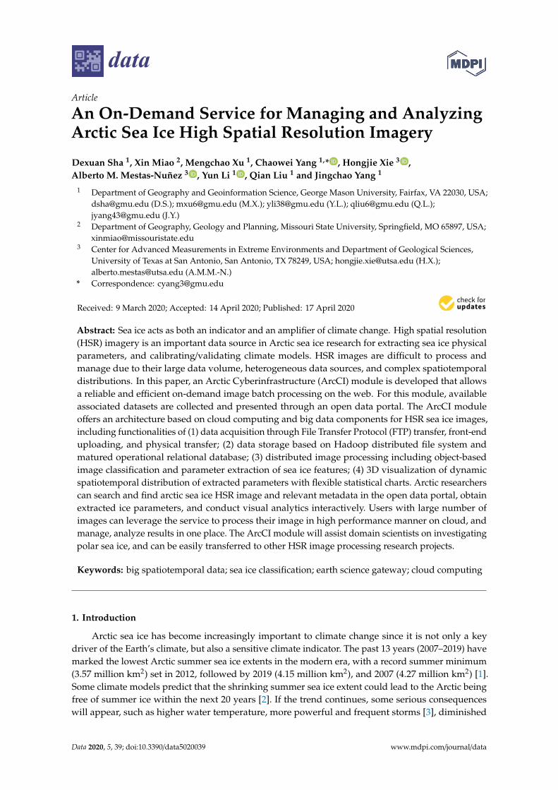
High spatial resolution image processing service is one of the major components in ArcCI.The algorithm is based on object-based classification of HSR sea ice images [29]. Our approach canextract all necessary sea ice features efficiently with limited human intervention, and the overallclassification accuracy can be as high as 95.5%. Three major steps of this algorithm (Figure 6) are listedas follows.

Data 2020, 5, x FOR PEER REVIEW 13 of 19

High spatial resolution image processing service is one of the major components in ArcCI. The algorithm is based on object-based classification of HSR sea ice images [29]. Our approach can extract all necessary sea ice features efficiently with limited human intervention, and the overall classification accuracy can be as high as 95.5%. Three major steps of this algorithm (Figure 6) are listed as follows.

Figure 6. Object-based Image Analysis (OBIA) workflow for sea ice classification.

Object-Based Image Segmentation

Most of the high-resolution sea ice photos were analyzed through pixel-based methods [15,16,30]. This method is based on pixel brightness values or spectral values, ignoring spatial autocorrelation, and generates ‘salt-and-pepper’ noise in the classification [31,32]. In contrast, object-based classification has been developed based on image segmentation, the process of partitioning an image into multiple objects or groups of pixels, making it more meaningful and easier to analyze [33,34]. This method not only considers spectral values but also spatial measurements that characterize the shape, texture, and contextual properties of the region so as to potentially improve classification accuracy [31]. The watershed segmentation algorithm is chosen for sea ice HSR images, followed by object merging through Region Adjacency Graphs (RAG). We developed a batch processing package in Python to handle large amounts of images.

Random Forest Classification

The outputs from the image segmentation above are individual objects or polygons. Spectral, texture, and shape features of each object can then be derived for each object and be imported into a random forest classifier for object-based classification. The random forest classifier is essentially a variant of the bagging tree ensemble classifier [35,36] through randomly selecting a subset of input features for each decision split. In this way, classification accuracy and feature importance can be evaluated by out-of-bag (OOB) estimations. This method is suitable for small sample problem such as object-based classification, and cloud-based multi-core parallel computing. A flexible classification scheme is the key to multitasking polar applications. We have defined a suitable classification scheme for high spatial resolution multi-band photos (Table 3).

Figure 6. Object-based Image Analysis (OBIA) workflow for sea ice classification.

Object-Based Image Segmentation

Most of the high-resolution sea ice photos were analyzed through pixel-based methods [15,16,30].This method is based on pixel brightness values or spectral values, ignoring spatial autocorrelation,and generates ‘salt-and-pepper’ noise in the classification [31,32]. In contrast, object-based classificationhas been developed based on image segmentation, the process of partitioning an image into multipleobjects or groups of pixels, making it more meaningful and easier to analyze [33,34]. This methodnot only considers spectral values but also spatial measurements that characterize the shape, texture,and contextual properties of the region so as to potentially improve classification accuracy [31].The watershed segmentation algorithm is chosen for sea ice HSR images, followed by object mergingthrough Region Adjacency Graphs (RAG). We developed a batch processing package in Python tohandle large amounts of images.

Random Forest Classification

The outputs from the image segmentation above are individual objects or polygons. Spectral,texture, and shape features of each object can then be derived for each object and be imported intoa random forest classifier for object-based classification. The random forest classifier is essentially avariant of the bagging tree ensemble classifier [35,36] through randomly selecting a subset of inputfeatures for each decision split. In this way, classification accuracy and feature importance can beevaluated by out-of-bag (OOB) estimations. This method is suitable for small sample problem such asobject-based classification, and cloud-based multi-core parallel computing. A flexible classificationscheme is the key to multitasking polar applications. We have defined a suitable classification schemefor high spatial resolution multi-band photos (Table 3).

Data 2020, 5, 39 13 of 18

Table 3. Classification scheme for object-based classification of sea ice photos.

# Class Name Class Description

1 Water Arctic ocean, objects are rather dark and smooth.

2 Submerged iceIce submerged under water along the edge, usually shown as color cyan or blue due to

mixed reflection from ice surface and water. Submerged ice and melt pond will becombined into ice/snow class for calculation of ice concentration.

3 Shadow

Darker objects on the ice/snow caused by ridges and low solar elevation angle. Mostly,shadow is usually on ice/snow and can be combined into ice/snow for calculation of iceconcentration. However, in some cases, shadows could also be on ponds that often are

adjacent to ridges. Therefore, further treatment about shadow on ice or ponds areneeded. Shadows will also be used for the calculation of ridge height.

4 Ice/snow Bright white objects due to high reflectance of ice/snow.

5 Melt pondPools of open water formed on sea ice. Melt pond will be used for calculation of fresh

water volume. Empirical equation to relate pond depth with pond area and distributionwill be examined based on our existing field data and ongoing field studies.

Polygon Neighbor Analysis

A major challenge is that submerged ice cannot be separated from melt ponds spectrally, sincethey have the same physical structure: water on the top, ice at the bottom. We can use polygon neighboranalysis to separate melt pond from submerged ice [29]. Additionally, submerged ice combined withwater can be used for sea-ice lead detection [37]. In this flexible classification scheme, submerged iceand melt ponds can be combined for albedo estimation if needed.

The functions could be easily expended with demands from the communities.The cyberinfrastructure and computing framework could support new functions with good compatibility.

4. Results

4.1. System Implementation

The ArcCI system leverages essential cloud computing resources including virtual machine (VM),storage/file system, and networking. The system incorporates web-based geoscience informationservices and analysis programming tools to customize the user interface for the Arctic sea ice study.The Openstack private cloud at GMU with 504-node computer cluster is used to support physical andcloud environment. 21 VM nodes of this cloud have been utilized to deploy a Spark cluster (v2.4.0 +

Hadoop v2.6.0) with one master node and 20 worker nodes, and the cluster resource is managed byYarn. Each VM is configured with 24 GPU cores, 4 TB storage, and 64 GB RAM on Centos 7.7 operatingsystem (OS). A public VM on AWS is utilized for providing data portal to integrate all web services onprivate cloud. All components on system can be extracted as cloud VM image resource to transfer so asto benefit other polar CI and polar science research.

On the Software as a Service (SaaS) level, the ArcCI portal Gateway has multiple loosely-coupledfunctionalities, so as to provide a life cycle service for HSR images from data uploading, storage,management, analysis, visualization, and sharing.

4.1.1. ArcCI Portal

We created the Arctic High Spatial Resolution (ArcHSR) Imagery Portal (Figure 7) to providemetadata for the sea ice community (http://archsri.stcenter.net/). Both collected and processed publicand longtail datasets are prepared for querying, browsing, and sharing. ArcHSR data portal also enabledata owner to register user account, organization page, and create dataset page. Multiple data licensesare used for data reusing, coping, publishing, distributing, transmitting, and adapting. All datasets canbe accessed and cited for non-commercial purposes. More importantly, a well-designed tagging andgrouping system is designed based on toponymy and sensor types, and it could be used to filter outthe most relevant dataset for researchers.

Data 2020, 5, 39 14 of 18

Data 2020, 5, x FOR PEER REVIEW 15 of 19

enable data owner to register user account, organization page, and create dataset page. Multiple data licenses are used for data reusing, coping, publishing, distributing, transmitting, and adapting. All datasets can be accessed and cited for non-commercial purposes. More importantly, a well-designed tagging and grouping system is designed based on toponymy and sensor types, and it could be used to filter out the most relevant dataset for researchers.

Figure 7. Screenshot of ArcHSR imagery open portal.

So far, 35 sea ice image collections were created and kept in ArcHSR open data portal from multiple data sources, including USGS, NASA, NSIDC, etc. Each collection is presented under individual page with description paragraph and metadata of author name, contact method, created time, data size and linkage and samples of raw data. The raw data format related to sea ice metadata includes HTML webpages, CSV tables with Point of Interest (POI) level records, unstructured text-based document, such PDF files and Word docs, and image example in TIFF and JPEG format.

4.1.2. Data Workflow for Multiple users

The workflow for users with different demands for sea ice research is shown in Figure 8. We defined three typical users with different motivations to use this service. First, the data owners have comprehensive control for uploading image data into data storage server, managing datasets under permissions, and processing images based on provided services. Second, researchers can upload metadata or extract geophysical parameter through visual image interpretation. Third, users without data can still access sea ice geophysical parameters for climate model validation, simulation and multi-platform data fusion. All visitors or users will be able to download extracted ice layers in geospatial data format for further data analysis and fusion process.

Figure 7. Screenshot of ArcHSR imagery open portal.

So far, 35 sea ice image collections were created and kept in ArcHSR open data portal from multipledata sources, including USGS, NASA, NSIDC, etc. Each collection is presented under individual pagewith description paragraph and metadata of author name, contact method, created time, data sizeand linkage and samples of raw data. The raw data format related to sea ice metadata includes HTMLwebpages, CSV tables with Point of Interest (POI) level records, unstructured text-based document,such PDF files and Word docs, and image example in TIFF and JPEG format.

4.1.2. Data Workflow for Multiple Users

The workflow for users with different demands for sea ice research is shown in Figure 8. We definedthree typical users with different motivations to use this service. First, the data owners have comprehensivecontrol for uploading image data into data storage server, managing datasets under permissions, andprocessing images based on provided services. Second, researchers can upload metadata or extractgeophysical parameter through visual image interpretation. Third, users without data can still access seaice geophysical parameters for climate model validation, simulation and multi-platform data fusion.All visitors or users will be able to download extracted ice layers in geospatial data format for furtherdata analysis and fusion process.

Data 2020, 5, x FOR PEER REVIEW 15 of 19

enable data owner to register user account, organization page, and create dataset page. Multiple data licenses are used for data reusing, coping, publishing, distributing, transmitting, and adapting. All datasets can be accessed and cited for non-commercial purposes. More importantly, a well-designed tagging and grouping system is designed based on toponymy and sensor types, and it could be used to filter out the most relevant dataset for researchers.

Figure 7. Screenshot of ArcHSR imagery open portal.

So far, 35 sea ice image collections were created and kept in ArcHSR open data portal from multiple data sources, including USGS, NASA, NSIDC, etc. Each collection is presented under individual page with description paragraph and metadata of author name, contact method, created time, data size and linkage and samples of raw data. The raw data format related to sea ice metadata includes HTML webpages, CSV tables with Point of Interest (POI) level records, unstructured text-based document, such PDF files and Word docs, and image example in TIFF and JPEG format.

4.1.2. Data Workflow for Multiple users

The workflow for users with different demands for sea ice research is shown in Figure 8. We defined three typical users with different motivations to use this service. First, the data owners have comprehensive control for uploading image data into data storage server, managing datasets under permissions, and processing images based on provided services. Second, researchers can upload metadata or extract geophysical parameter through visual image interpretation. Third, users without data can still access sea ice geophysical parameters for climate model validation, simulation and multi-platform data fusion. All visitors or users will be able to download extracted ice layers in geospatial data format for further data analysis and fusion process.

Figure 8. Users’ views on functionalities.

Data 2020, 5, 39 15 of 18

4.1.3. Visualization Tool

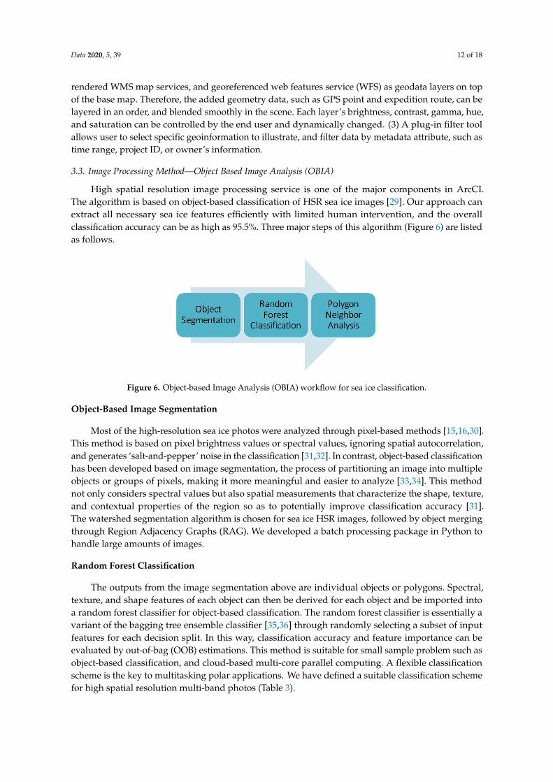
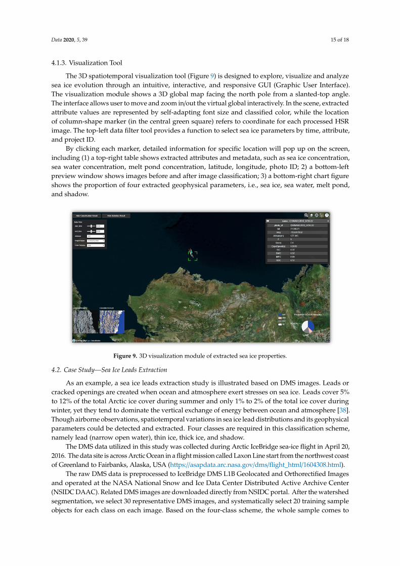
The 3D spatiotemporal visualization tool (Figure 9) is designed to explore, visualize and analyzesea ice evolution through an intuitive, interactive, and responsive GUI (Graphic User Interface).The visualization module shows a 3D global map facing the north pole from a slanted-top angle.The interface allows user to move and zoom in/out the virtual global interactively. In the scene, extractedattribute values are represented by self-adapting font size and classified color, while the locationof column-shape marker (in the central green square) refers to coordinate for each processed HSRimage. The top-left data filter tool provides a function to select sea ice parameters by time, attribute,and project ID.

By clicking each marker, detailed information for specific location will pop up on the screen,including (1) a top-right table shows extracted attributes and metadata, such as sea ice concentration,sea water concentration, melt pond concentration, latitude, longitude, photo ID; 2) a bottom-leftpreview window shows images before and after image classification; 3) a bottom-right chart figureshows the proportion of four extracted geophysical parameters, i.e., sea ice, sea water, melt pond,and shadow.

Data 2020, 5, x FOR PEER REVIEW 16 of 19

Figure 8. Users’ views on functionalities.

4.1.3. Visualization Tool

The 3D spatiotemporal visualization tool (Figure 9) is designed to explore, visualize and analyze sea ice evolution through an intuitive, interactive, and responsive GUI (Graphic User Interface). The visualization module shows a 3D global map facing the north pole from a slanted-top angle. The interface allows user to move and zoom in/out the virtual global interactively. In the scene, extracted attribute values are represented by self-adapting font size and classified color, while the location of column-shape marker (in the central green square) refers to coordinate for each processed HSR image. The top-left data filter tool provides a function to select sea ice parameters by time, attribute, and project ID.

By clicking each marker, detailed information for specific location will pop up on the screen, including (1) a top-right table shows extracted attributes and metadata, such as sea ice concentration, sea water concentration, melt pond concentration, latitude, longitude, photo ID; 2) a bottom-left preview window shows images before and after image classification; 3) a bottom-right chart figure shows the proportion of four extracted geophysical parameters, i.e., sea ice, sea water, melt pond, and shadow.

Figure 9. 3D visualization module of extracted sea ice properties.

4.2. Case Study—Sea Ice Leads Extraction

As an example, a sea ice leads extraction study is illustrated based on DMS images. Leads or cracked openings are created when ocean and atmosphere exert stresses on sea ice. Leads cover 5% to 12% of the total Arctic ice cover during summer and only 1% to 2% of the total ice cover during winter, yet they tend to dominate the vertical exchange of energy between ocean and atmosphere [38]. Though airborne observations, spatiotemporal variations in sea ice lead distributions and its geophysical parameters could be detected and extracted. Four classes are required in this classification scheme, namely lead (narrow open water), thin ice, thick ice, and shadow.

The DMS data utilized in this study was collected during Arctic IceBridge sea-ice flight in April 20, 2016. The data site is across Arctic Ocean in a flight mission called Laxon Line start from the northwest coast of Greenland to Fairbanks, Alaska, USA (https://asapdata.arc.nasa.gov/dms/flight_html/1604308.html).

The raw DMS data is preprocessed to IceBridge DMS L1B Geolocated and Orthorectified Images and operated at the NASA National Snow and Ice Data Center Distributed Active Archive Center (NSIDC DAAC). Related DMS images are downloaded directly from NSIDC portal. After the watershed segmentation, we select 30 representative DMS images, and systematically select 20

Figure 9. 3D visualization module of extracted sea ice properties.

4.2. Case Study—Sea Ice Leads Extraction

As an example, a sea ice leads extraction study is illustrated based on DMS images. Leads orcracked openings are created when ocean and atmosphere exert stresses on sea ice. Leads cover 5%to 12% of the total Arctic ice cover during summer and only 1% to 2% of the total ice cover duringwinter, yet they tend to dominate the vertical exchange of energy between ocean and atmosphere [38].Though airborne observations, spatiotemporal variations in sea ice lead distributions and its geophysicalparameters could be detected and extracted. Four classes are required in this classification scheme,namely lead (narrow open water), thin ice, thick ice, and shadow.

The DMS data utilized in this study was collected during Arctic IceBridge sea-ice flight in April 20,2016. The data site is across Arctic Ocean in a flight mission called Laxon Line start from the northwest coastof Greenland to Fairbanks, Alaska, USA (https://asapdata.arc.nasa.gov/dms/flight_html/1604308.html).

The raw DMS data is preprocessed to IceBridge DMS L1B Geolocated and Orthorectified Imagesand operated at the NASA National Snow and Ice Data Center Distributed Active Archive Center(NSIDC DAAC). Related DMS images are downloaded directly from NSIDC portal. After the watershedsegmentation, we select 30 representative DMS images, and systematically select 20 training sampleobjects for each class on each image. Based on the four-class scheme, the whole sample comes to

Data 2020, 5, 39 16 of 18

2400 objects. These training samples are fed in the random forest classifier to classify all four leadrelated classes in ArcCI. The ArcCI module is run under the distributed computing environment onspark cluster (v2.2.0 + Hadoop V2.6.0) which consists of one master node and 4 worker nodes, andYarn is used as the cluster resource manager. Each node is configured with 24 CPU cores (2.35 GHz)and 24 GB RAM on CentOS 7.2 and connected with 20 GB InfiniBand (GPS).

Six example classification results are shown in Figure 10. Comparing to visual examination, weconclude that 1) the object-based classification model is effective for sea ice classification for HSR images;and 2) distributed computing framework enables the image analysis pipeline viable in cloud-based bigdata system.

Data 2020, 5, x FOR PEER REVIEW 17 of 19

training sample objects for each class on each image. Based on the four-class scheme, the whole sample comes to 2400 objects. These training samples are fed in the random forest classifier to classify all four lead related classes in ArcCI. The ArcCI module is run under the distributed computing environment on spark cluster (v2.2.0 + Hadoop V2.6.0) which consists of one master node and 4 worker nodes, and Yarn is used as the cluster resource manager. Each node is configured with 24 CPU cores (2.35 GHz) and 24 GB RAM on CentOS 7.2 and connected with 20 GB InfiniBand (GPS).

Six example classification results are shown in Figure 10. Comparing to visual examination, we conclude that 1) the object-based classification model is effective for sea ice classification for HSR images; and 2) distributed computing framework enables the image analysis pipeline viable in cloud-based big data system.

Figure 10. Visual classification results for four-class schema.

5. Conclusions

Sea ice plays an important role in climate change. HSR sea ice images captured by satellites or airplanes provide detailed observational data for extracting geophysical attributes of sea ice features, such as floe or melt pond shape, distribution, and coverage. HSR images, however, pose a serious challenge for discovering spatiotemporal patterns of sea ice from this heterogeneous big data in a timely manner [39]. We design and build the ArcCI system based on cloud computing to handle this big data challenge. The ArcCI web service provide a one-stop platform for HSR image management (storage, archival retrieval/access, and backup), analysis (image processing, classification, and statistics), and visualization.

In the future, the ArcCI system will be enhanced [40] by (1) including more scalable computing resources for the dynamic on-demand Web service, which would enable users to process and analyze HSR images using pixel-based or object-based methods; (2) integrating data fusion analysis by combining low spatial resolution satellite images to extract geophysical properties at different scales; (3) integrating more data visualization functions for data exploratory analysis; and (4) optimizing high performance computing for big data processing by taking advantage of Spark in distributed memory or other advantage processing framework.

Author Contributions: Conceptualization, A.M.M-N., X.M., H.X., and C.Y.; methodology, D.S., X.M. and M.X., C.Y.; software, D.S. and X.M.; investigation, D.S. and M.X.; resources, Y.L., Q.L. and J.Y.; data curation, D.S.; writing—original draft preparation, D.S. and X.M.; writing—review and editing, H.X. and C.Y.; visualization, D.S.; project administration, H.X.; funding acquisition, C.Y. All authors have read and agreed to the published version of the manuscript.

Figure 10. Visual classification results for four-class schema.

5. Conclusions

Sea ice plays an important role in climate change. HSR sea ice images captured by satellites orairplanes provide detailed observational data for extracting geophysical attributes of sea ice features,such as floe or melt pond shape, distribution, and coverage. HSR images, however, pose a seriouschallenge for discovering spatiotemporal patterns of sea ice from this heterogeneous big data in atimely manner [39]. We design and build the ArcCI system based on cloud computing to handle thisbig data challenge. The ArcCI web service provide a one-stop platform for HSR image management(storage, archival retrieval/access, and backup), analysis (image processing, classification, and statistics),and visualization.

In the future, the ArcCI system will be enhanced [40] by (1) including more scalable computingresources for the dynamic on-demand Web service, which would enable users to process and analyzeHSR images using pixel-based or object-based methods; (2) integrating data fusion analysis bycombining low spatial resolution satellite images to extract geophysical properties at different scales;(3) integrating more data visualization functions for data exploratory analysis; and (4) optimizing highperformance computing for big data processing by taking advantage of Spark in distributed memoryor other advantage processing framework.

Author Contributions: Conceptualization, A.M.M.-N., X.M., H.X., and C.Y.; methodology, D.S., X.M. and M.X.,C.Y.; software, D.S. and X.M.; investigation, D.S. and M.X.; resources, Y.L., Q.L. and J.Y.; data curation, D.S.;writing—original draft preparation, D.S. and X.M.; writing—review and editing, H.X. and C.Y.; visualization, D.S.;project administration, H.X.; funding acquisition, C.Y. All authors have read and agreed to the published versionof the manuscript.

Data 2020, 5, 39 17 of 18

Funding: This research was funded by NSF under “Collaborative Research: Elements: Data: HDR: DevelopingOn-Demand Service Module for Mining Geophysical Properties of Sea Ice from High Spatial Resolution Imagery”,grant number 1835507 (GMU), 1835784 (UTSA), 1835512 (MSU).

Acknowledgments: The authors are thankful with Timothy Wu for providing technical support on data andliterature collection and online data services, Victoria Dombrowik for analyzing open-source packages available inthe market and the community, and Zifu Wang for assisting with front-end development.

Conflicts of Interest: The authors declare no conflict of interest.

References

1. Parkinson, C.L. A 40-y record reveals gradual Antarctic sea ice increases followed by decreases at ratesfar exceeding the rates seen in the Arctic. Proc. Natl. Acad. Sci. USA 2019, 116, 14414–14423. [CrossRef][PubMed]

2. Marshall, M. Arctic ice low kicks off a cascade of tipping points. New Sci. 2013, 217, 6–7. [CrossRef]3. Parkinson, C.L.; Comiso, J.C. On the 2012 record low Arctic sea ice cover: Combined impact of preconditioning

and an August storm. Geophys. Res. Lett. 2013, 40, 1356–1361. [CrossRef]4. Jeffries, M.O.; Overland, J.E.; Perovich, D.K. The Arctic shifts to a new normal. Phys. Today 2013, 66, 35–40.

[CrossRef]5. Silverman, J. Why Is Arctic Ice Melting 50 Years Too Fast? Available online: http://science.howstuffworks.

com/environmental/earth/geophysics/arctic-ice.htm (accessed on 5 September 2019).6. NRC. Earth Science and Applications from Space: National Imperatives for the Next Decade and beyond; The National

Academies Press: Washington, DC, USA, 2007.7. Wu, X.; Zhu, X.; Wu, G.-Q.; Ding, W. Data mining with big data. IEEE Trans. Knowl. Data Eng. 2014, 26,

97–107.8. Flocco, D.; Feltham, D.L. A continuum model of melt pond evolution on Arctic sea ice. J. Geophys. Res.

Space Phys. 2007, 112, C08016. [CrossRef]9. Kwok, R.; Untersteiner, N. New High-Resolution Images of Summer Arctic Sea Ice. EOS 2011, 92, 53–54.

[CrossRef]10. Dominguez, R. IceBridge DMS L1B Geolocated and Orthorectified Images; NASA National Snow and Ice Data

Center Distributed Active Archive Center: Boulder, CO, USA, 2010.11. Perovich, D.K.; Grenfell, T.C.; Richter-Menge, J.A.; Light, B.; Tucker, W.B.; Eicken, H. Thin and thinner:

Sea ice mass balance measurements during SHEBA. J. Geophys. Res. Space Phys. 2003, 108. [CrossRef]12. Perovich, D.K.; Grenfell, T.C.; Light, B.; Elder, B.C.; Harbeck, J.; Polashenski, C.; Tucker, W.B., III; Stelmach, C.

Transpolar observations of the morphological properties of Arctic sea ice. J. Geophys. Res. Space Phys. 2009,114. [CrossRef]

13. Ruibo, L.; Zhijun, L.; Bin, C.; QingHua, Y.; Na, L. Investigation of the thermodynamic processes of a floe-leadsystem in the central Arctic during later summer. Polar Res. 2011, 22, 10–16.

14. Lei, R.; Zhang, Z.; Matero, I.; Cheng, B.; Li, Q.; Huang, W. Reflection and transmission of irradiance by snowand sea ice in the central Arctic Ocean in summer 2010. Polar Res. 2012, 31, 17325. [CrossRef]

15. Lu, P.; Li, Z.; Cheng, B.; Lei, R.; Zhang, R. Sea ice surface features in Arctic summer 2008: Aerial observations.Remote. Sens. Environ. 2010, 114, 693–699. [CrossRef]

16. Renner, A.H.; Dumont, M.; Beckers, J.; Gerland, S.; Haas, C. Improved characterisation of sea ice usingsimultaneous aerial photography and sea ice thickness measurements. Cold Reg. Sci. Technol. 2013, 92, 37–47.[CrossRef]

17. Xie, H.; Lei, R.; Ke, C.; Wang, H.; Li, Z.; Zhao, J.; Ackley, S.F. Summer sea ice characteristics and morphologyin the Pacific sector as observed during the CHINARE 2010 cruise. Cryosphere 2013, 7, 1057–1072. [CrossRef]

18. Johnson, G.W.; Gaylord, A.G.; Franco, J.C.; Cody, R.P.; Brady, J.J.; Manley, W.; Dover, M.; Garcia-Lavigne, D.;Score, R.; Tweedie, C.E. Development of the Arctic Research Mapping Application (ARMAP): Interoperabilitychallenges and solutions. Comput. Geosci. 2011, 37, 1735–1742. [CrossRef]

19. Khalsa, S.J.; Parsons, M.; Yarmey, L.; Truslove, I.; Pearlman, J.; Boldrini, E. The Advanced Cooperative ArcticData and Information Service (ACADIS). In Proceedings of the EGU General Assembly Conference Abstracts,Vienna, Austria, 7–12 April 2013.

Data 2020, 5, 39 18 of 18

20. Institute, N.P. Norwegian Polar Data Centre. Available online: https://data.npolar.no/ (accessed on5 February 2020).

21. Jiang, Y.; Li, J.; Yang, C.; Huang, Q. Visualizing 5D environmental data, Environmental Modeling andSoftware. Environ. Model. Softw. 2014, in press.

22. Li, Z.; Yang, C.; Liu, K.; Sun, M. MaaS: Model as a Service. Comput. Environ. Urban Syst. 2014, 61, 141–152.[CrossRef]

23. Yang, C.; Sun, M.; Liu, K.; Huang, Q.; Li, Z.; Gui, Z.; Jiang, Y.; Xia, J.; Yu, M.; Xu, C. Contemporary computingtechnologies for processing big spatiotemporal data. In Space-Time Integration in Geography and GIScience;Springer: Berlin/Heidelberg, Germany, 2015; pp. 327–351.

24. Huang, Q.; Yang, C.; Benedict, K.; Chen, S.; Rezgui, A.; Xie, J. Utilize cloud computing to support dust stormforecasting. Int. J. Digit. Earth 2013, 6, 338–355. [CrossRef]

25. Yang, C.; Huang, Q. Spatial Cloud Computing: A Practical Approach; CRC Press: Boca Raton, FL, USA, 2013.26. Gorelick, N.; Hancher, M.; Dixon, M.; Ilyushchenko, S.; Thau, D.; Moore, R. Google Earth Engine:

Planetary-scale geospatial analysis for everyone. Remote. Sens. Environ. 2017, 202, 18–27. [CrossRef]27. Gui, Z.; Yang, C.; Xia, J.; Li, J.; Rezgui, A.; Sun, M.; Xu, Y.; Fay, D. A visualization-enhanced graphical user

interface for geospatial resource discovery. Ann. GIS 2013, 19, 109–121. [CrossRef]28. Li, Z.; Yang, C.P.; Wu, H.; Li, W.; Miao, L. An optimized framework for seamlessly integrating OGC Web

Services to support geospatial sciences. Int. J. Geogr. Inf. Sci. 2011, 25, 595–613. [CrossRef]29. Miao, X.; Xie, H.; Ackley, S.F.; Perovichcd, D.K.; Ke, C. Object-Based Detection of Arctic Sea Ice and Melt

Ponds Using High Spatial Resolution Aerial Photographs. Cold Reg. Sci. Technol. 2015, 119, 211–222.[CrossRef]

30. Weissling, B.; Ackley, S.; Wagner, P.; Xie, H. EISCAM—Digital image acquisition and processing for sea iceparameters from ships. Cold Reg. Sci. Technol. 2009, 57, 49–60. [CrossRef]

31. Liu, D.; Xia, F. Assessing object-based classification: Advantages and limitations. Remote. Sens. Lett. 2010, 1,187–194. [CrossRef]

32. Xie, H.; Tian, Y.Q.; Granillo, J.A.; Keller, G.R. Suitable remote sensing method and data for mapping andmeasuring active crop field. Int. J. Remote Sens. 2007, 28, 395–411. [CrossRef]

33. Shapiro, L.; Stockman, G. Computer Vision. Prentice Hall. Inc.: Upper Saddle River, NJ, USA, 2001.34. Hussain, M.; Chen, D.M.; Cheng, A.; Wei, H.; Stanley, D. Change detection from remotely sensed images:

From pixel-based to object-based approaches. ISPRS J. Photogramm. Remote Sens. 2013, 80, 91–106. [CrossRef]35. Breiman, L.; Friedman, J.H.; Olshen, R.A.; Stone, C.J. Classification and regression trees. Belmont, CA:

Wadsworth. Int. Group 1984, 432, 151–166.36. Breiman, L. Random forests. Mach. Learn. 2001, 45, 5–32. [CrossRef]37. Onana, V.D.; Kurtz, N.T.; Farrell, S.L.; Koenig, L.S.; Studinger, M.; Harbeck, J.P. A Sea-Ice Lead Detection

Algorithm for Use With High-Resolution Airborne Visible Imagery. IEEE Trans. Geosci. Remote. Sens 2013, 51,38–56. [CrossRef]

38. Wang, Q.; Danilov, S.; Jung, T.; Kaleschke, L.; Wernecke, A. Sea ice leads in the Arctic Ocean: Model assessment,interannual variability and trends. Geophys. Res. Lett. 2016, 43, 7019–7027. [CrossRef]

39. Yu, M.; Bambacus, M.; Cervone, G.; Clarke, K.; Duffy, D.; Huang, Q.; Li, J.; Li, W.; Li, Z.; Liu, Q.; et al.Spatiotemporal event detection: A review. Int. J. Digit. Earth 2020, 1–27. [CrossRef]

40. Yang, C.; Clarke, K.; Shekhar, S.; Tao, C.V. Big Spatiotemporal Data Analytics: A research and innovationfrontier. Int. J. Geogr. Inf. Sci. 2019, 1–14. [CrossRef]

© 2020 by the authors. Licensee MDPI, Basel, Switzerland. This article is an open accessarticle distributed under the terms and conditions of the Creative Commons Attribution(CC BY) license (http://creativecommons.org/licenses/by/4.0/).