IPN Progress Report 42-154 August 15, 2003

An Optical Array Receiver for Deep-SpaceCommunication through Atmospheric

TurbulenceV. Vilnrotter,1 C.-W. Lau,1 M. Srinivasan,1 R. Mukai,1 and K. Andrews1

The theoretical foundations of an optical array receiver consisting of relativelysmall telescopes are developed and analyzed. It is shown that optical array re-ceivers can be designed to perform as well as a large single-aperture receiver onthe ground, while enjoying significant advantages in terms of operational reliabil-ity, ease of future expansion to achieve greater capacity, and further advantages interms of cost and implementation due to the highly parallel architecture inherentin the array design. Optical array receivers for deep-space communication appli-cations are analyzed using the accepted modal analysis for background radiation;however, the signal fields are represented using a novel aperture-plane expansionthat takes into account the characteristics of atmospheric turbulence. It is shown,based on this analysis, that for ground-based reception the number of array ele-ments can be increased without suffering any performance degradation, as long asthe telescope diameters exceed the coherence length of the atmosphere. Maximum-likelihood detection of turbulence-degraded signal fields using an array of telescopes,each equipped with its own focal-plane detector array to mitigate turbulence effects,is developed for the case of pulse-position modulated signals observed in the pres-ence of background radiation. The performance of optical array receivers then iscompared to single-aperture receivers with diameters ranging from 4 to 8 meters,both in the presence of turbulence relevant to ground-based reception and in ahypothetical turbulence-free environment; it is shown that without atmosphericturbulence to break up the signal fields prior to detection, as would be the casein space, single-aperture receivers outperform receiver arrays whenever significantbackground radiation is present. However, for ground-based reception of deep-spacesignals, we demonstrate that the number of array elements can be as great as sev-eral thousand without incurring any performance degradation relative to a largesingle-aperture optical receiver.

1 Communications Systems and Research Section.

The research described in this publication was carried out by the Jet Propulsion Laboratory, California Institute ofTechnology, under a contract with the National Aeronautics and Space Administration.

1

I. Introduction

Earth-based reception of deep-space optical signals using an array of relatively small telescopes togetherwith high-speed digital signal processing is a viable alternative to large-aperture telescopes for receivingdeep-space optical signals. Large-aperture telescopes are costly to build and operate, and inherently sufferfrom single-point failure in case of malfunction, thus jeopardizing precious data. Performance of a properlydesigned array tends to degrade gracefully in case of element failures, even without replacement, but thearray approach also provides the option to switch in spare telescopes in case of failure, without a significantincrease in cost. However, the equivalence of the array receiver and the single large telescope underoperating conditions of interest remains to be demonstrated; establishing that theoretical equivalenceand clarifying the similarities and differences between the two approaches is the goal of this article.

The premise of a single-aperture optical receiver for deep-space telemetry is to employ one large(approximately 10-meter) primary reflector, possibly segmented, with custom optics designed to focusthe turbulence-degraded optical fields onto a large-area detector. Due to the large mirror size, diffraction-limited performance is difficult to attain at reasonable cost, and in addition the large optics require amassive and costly mechanical support and tracking system. If, instead, we consider building an opticalreceiver array using relatively small but high-quality off-the-shelf telescopes, we will be able to meetrequirements in a cost-effective manner with the added benefit that development, testing, and evaluationcosts can be greatly reduced. This follows because with an array all the elements are identical, and thefundamental interconnectivity and arraying concepts can be demonstrated with just a few elements; forexample, a small array consisting of two or three telescopes can be used to demonstrate virtually all ofthe necessary arraying concepts relatively cheaply, and the results can be extrapolated with confidenceto a much larger array. Not so with a receiver relying on a single huge reflector; a single large-aperturetelescope has additional unique features and problems that a small telescope prototype will not reveal.The difficulty of constructing and aligning a large optical telescope, segmented aperture or otherwise, isin itself a daunting task, exacerbated by the additional problems that gravitational loading produces onthe backup structure and drive mechanism.

In addition to a favorable cost and risk trade-off, the optical array receiver approach has advantages interms of implementation complexity and performance for several key communications functions that needto be clarified and evaluated. These characteristics can best be explained in terms of an array receivermodel that emphasizes the communications aspects of the optical array. We begin by developing theunderlying concepts governing the behavior of optical arrays. Next, similarities and differences betweensingle-aperture and array telescopes designed for reception of deep-space telemetry will be explored,followed by a detailed investigation of communications performance. We conclude with a comparisonof array receivers with the more conventional large-aperture optical receiver under realistic operatingconditions.

II. The Optical Array Receiver Concept

The essential difference between a single-aperture optical communications receiver and an opticalarray receiver is that a single aperture focuses all of the light energy it collects onto the surface ofan optical detector before detection, whereas an array receiver focuses portions of the total collectedenergy onto separate detectors, optically detects each fractional energy component, and then combinesthe electrical signal from the array of detector outputs to form the observable, or “decision statistic”used to decode the telemetry signal. Thus, an optical interferometer that attempts to synthesize a hugeaperture with a few sparsely spaced elements to increase resolution really counts as a single-aperturereceiver according to this definition, even though it appears to be composed of disconnected elementsmuch like an array. The point is that with an interferometer the light from the interferometer elementsis combined coherently before detection, whereas in a communications array, according to our definition,light is detected at each element first, followed by post-detection processing to construct the desiredsignal. A single-aperture receiver need not be constructed from a single monolithic glass lens or reflector

2

element; large modern telescopes generally are constructed from hexagonal segments with each surfaceplaced near its neighbors and monitored to form a single parabolic surface. Alternatively, this type ofconstruction can be thought of as a “dense interferometer,” where the high-resolution partial image dueto the distant outer elements is filled in completely to reconstruct the image in real time (instead of theconventional “sparse interferometer,” where post-processing typically is required to reconstruct the imageafter the observation). If the image of a point source were formed using every segment of the surface andthen detected, that collection of segments would be considered a single-aperture receiver. However, if thefocal spot of each segment were separated from the rest and detected with a separate detector element orfocal-plane detector array, that would constitute an array receiver in the framework of our definition. Notethat a focal-plane array in a single telescope might be construed as an optical array receiver under thisdefinition, but the intent is for there to be multiple apertures. This construction serves as a convenientconceptual vehicle to illustrate the similarities and differences between single-aperture and multi-aperturearray receivers.

A conceptual block diagram of an optical array receiver suitable for deep-space telemetry reception isshown in Fig. 1, intended to identify the key components required for array receiver operation. The mostconspicuous feature of an optical array receiver is a large number of small- to medium-sized telescopes,with the individual apertures and number of telescopes designed to make up the desired total collectingarea. This array of telescopes is envisioned to be fully computer controlled via the user interface, andpredict-driven to achieve rough pointing and tracking of the desired spacecraft. Fine-pointing and trackingfunctions then take over to keep each telescope pointed towards the source despite imperfect pointingpredicts, telescope drive errors, and vibration caused by light wind.

The optical signal collected by each telescope is focused onto a detector array located in the focal plane,designated as the focal-plane array, or FPA. Despite atmospheric turbulence degrading the coherence ofthe received signal fields and interfering background radiation entering the receiver along with the signalwithin the passband of the optical pre-detection filter, the FPA and associated digital signal-processingelectronics extract real-time pointing information, keeping the centroid of the turbulent time-varying

Real-Time DelayCompensation

Array Combining,Sync, Tracking

Symbol Detection,Decoding

REAL-TIME TRACKING UPDATES Drive Correction Tip-Tilt Mirror Assembly

ADAPTIVE SUBARRAYS

ARRAY SIGNAL PROCESSING

TELESCOPE ARRAY

USER INTERFACE:DECODED DATA

FEEDBACK

FPA SIGNAL PROCESSING:

Fig. 1. Conceptual design of an optical array receiver, illustrating key functions required for array reception: thetelescope array; focal-plane pre-processing of the signal at each telescope; and the additional array processingneeded to combine the pre-processed signals and decode the received data.

PREDICTS

DSP CONTROL

3

signal centered over the FPA. This is accomplished in two steps: first, large accumulated pointing errorsare fed back to the telescope drive assembly, repointing the entire instrument; and second, small excursionsof the signal distribution from the center of the array are corrected via a fast-response tip–tilt mirror thatresponds to real-time pointing updates generated by the FPA electronics. In addition, the short-termaverage signal energy over each detector element is measured and used to implement various adaptivebackground-suppression algorithms to improve or optimize the communications performance of the entirearray.

The electrical signals generated at each telescope by the FPA signal-processing assembly are collected ata central array signal-processing station, where the final operations necessary for data decoding are carriedout. The relative time delay between signals from various telescopes is measured and removed, effectivelyaligning each signal stream in time before further processing is carried out. The delay-compensatedsignals then are combined in a manner to optimize array performance, and further processed to affectsymbol synchronization, frame synchronization, Doppler compensation, and to effectively maintain lockbetween the combined signal and the receiver time frame. At this point, the transmitted channel symbolsare detected, and the decoding operation begins. The detected channel symbols now could be handedover to a hard-decision decoder or various forms of soft-decision decoding could be implemented throughthe use of additional side information along with the detected symbols. The channel symbols detected bythe array receiver also may be used to aid the delay compensation, array combining, and synchronizationoperations.

III. Aperture-Plane Expansions

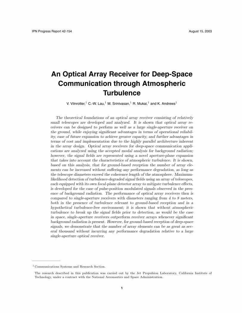
It is common practice in the optical communications literature to expand random fields at the telescopeaperture into spatial modes that are closely related to diffraction-limited fields of view, clustered to forma complete orthonormal set of functions that essentially samples the field of view (FOV) of the receiver.This concept is illustrated in Fig. 2, where a cluster of diffraction-limited fields of view (denoted Ωdl) isshown collecting light energy from both signal and background radiation with slightly different angles ofarrival. If it can be shown that each element of the set of spatial modes satisfies an integral equationwhose kernel is the field coherence function over the aperture, then each sample function of the field canbe expanded into an orthonormal series with uncorrelated coefficients, also known as a Karhounen–Loeveexpansion [1].

Fig. 2. Plane-wave expansion of aperture-plane fields: diffraction-limitedFOV interpretation.

BACKGROUNDFIELDS

SIGNALFIELDS

D

dlΩ

dlK Ω

4

When applying this model to the array receiver, it is more appropriate to view the received turbulence-degraded optical fields as “frozen” over time scales of milliseconds, the characteristic time scale of tur-bulence, during which time a great many optical data symbols are received. It is advantageous to vieweach sample function of the received field as a frozen realization of a two-dimensional field, representing acertain epoch in time over which the stationary model applies, as a deterministic two-dimensional func-tion defined over the aperture plane of the receiver. This enables the application of well-known samplingtheory to the fields, resulting in a model that clarifies the array receiver concept and contributes to thedevelopment of a useful engineering model.

Plane-wave expansions are especially useful for characterizing the effects of background radiation. InFig. 2, both signal and background power are shown entering the receiver through each diffraction-limitedFOV. If the diameter of the receiver is smaller than the coherence length of the signal field (a conditionthat can be met in the vacuum of space or even on the ground with very small apertures), then allof the signal energy is concentrated into a diffraction-limited point-spread function (PSF) in the focalplane. In effect, the signal appears to originate from a point source an infinite distance from the receiver.For the case of receiving spatially coherent signal fields, the signal power collected by a diffraction-limited telescope under ideal conditions is therefore proportional to the collecting area. The model forbackground radiation is somewhat more complicated, since background radiation is an extended sourcewith respect to the narrow FOV of typical optical receivers. Surprisingly, the background power collectedby a diffraction-limited telescope does not depend on the collecting area, but instead is a constant thatdepends only on the brightness of the source and the bandwidth of the optical filter at the wavelengthof interest, λ. This can be shown by examining the units of the spectral radiance function, N(λ), usedto quantify background radiation: the units of the spectral radiance functions are power (microwatts)per receiver area (square meters), field of view (steradians), and optical filter bandwidth (angstroms ornanometers). The background power collected by a diffraction-limited receiver is given by [3]

Pb = N(λ)∆λΩdlAr

where ∆λ is the optical filter bandwidth and Ar is the collecting area. Since the diffraction-limited fieldof view is inversely related to area, i.e., Ωdl ≈ λ2/Ar, we have

P ∗b ≈ N(λ)∆λλ2

and therefore the background power collected by a diffraction-limited receiver, P ∗b , is independent of

receiver area. Therefore, all diffraction-limited receivers of whatever size collect the same backgroundpower when observing a given background distribution, independent of receiver collecting area.

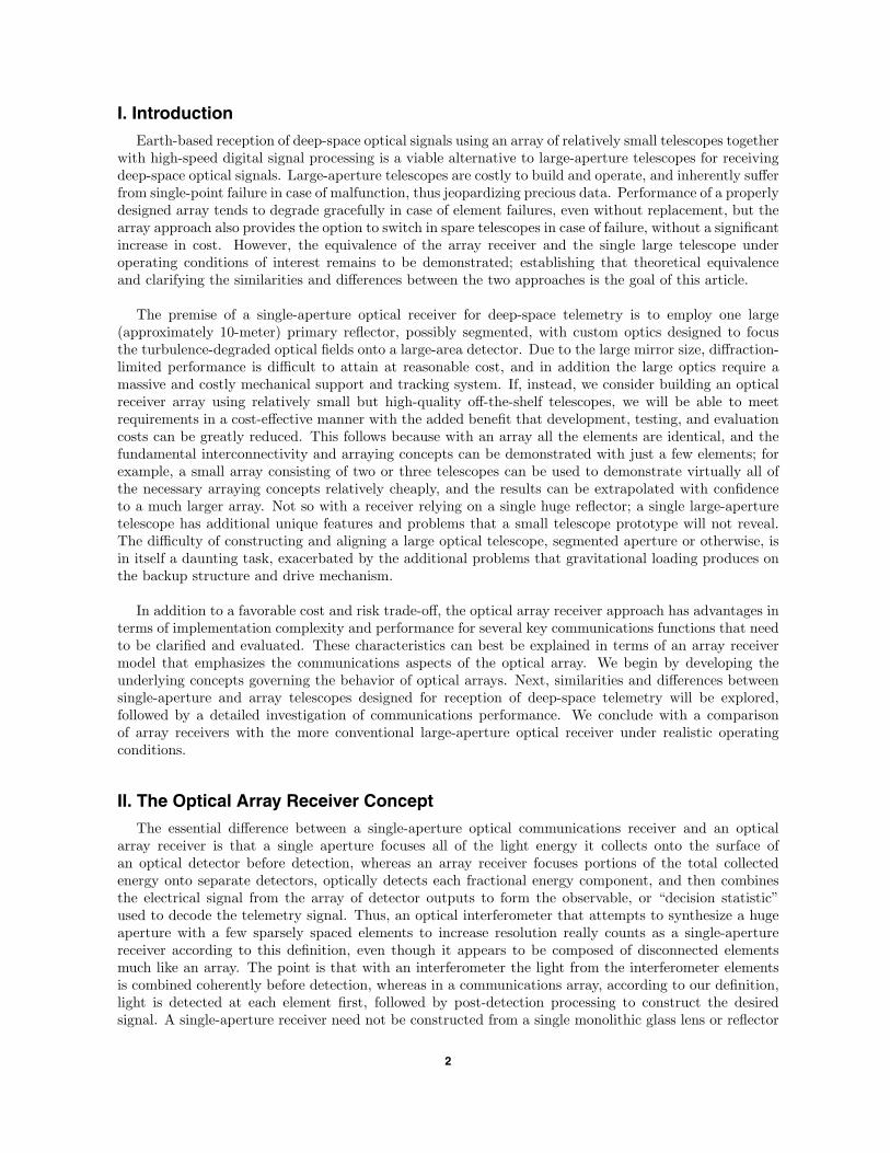
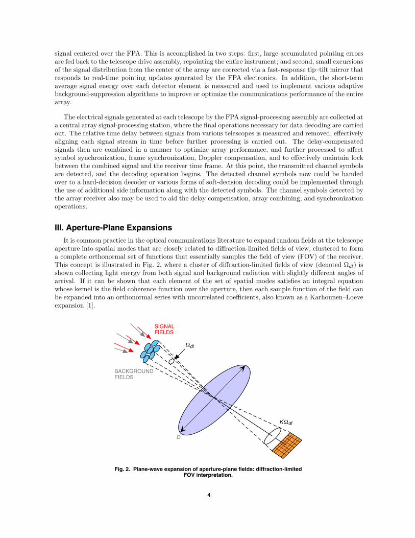
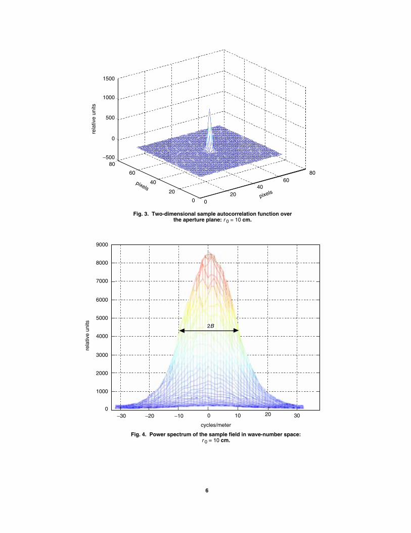
The distorted optical fields resulting from atmospheric turbulence are necessarily bandlimited, sincethe “image” of a point source observed through turbulence is of finite extent. This conclusion is based onthe observation that any complex field distribution over the aperture plane is the Fourier transform of thecomplex “image” function generated in the focal plane [4,5], which therefore represents the wave-numberspace of the aperture. In order to determine the extent of significant wave numbers of representativeoptical field distributions, sample functions generated from Kolmogorov phase screens were analyzed.Representative examples of the resulting aperture-plane coherence function and its Fourier transform,representing the two-dimensional power spectrum of the field in wave -number space, are shown in Figs. 3and 4, for the case of 10-cm atmospheric coherence length, or r0 = 0.1 meter.

If we can show that the received fields over the aperture are wavenumber-limited two-dimensionalfunctions, then we can invoke a two-dimensional version of the sampling theorem, as described in [5].This enables the expansion of the received fields using two-dimensional sampling functions, analogous to

5

1500

1000

500

0

−50080

60

40

20

0

8060

4020

0

rela

tive

units

pixels

pixels

Fig. 3. Two-dimensional sample autocorrelation function overthe aperture plane: r 0 = 10 cm.

9000

8000

7000

6000

5000

4000

3000

2000

1000

0−10 0 10 20 30

Fig. 4. Power spectrum of the sample field in wave-number space:r 0 = 10 cm.

cycles/meter

rela

tive

units 2B

−20−30

6

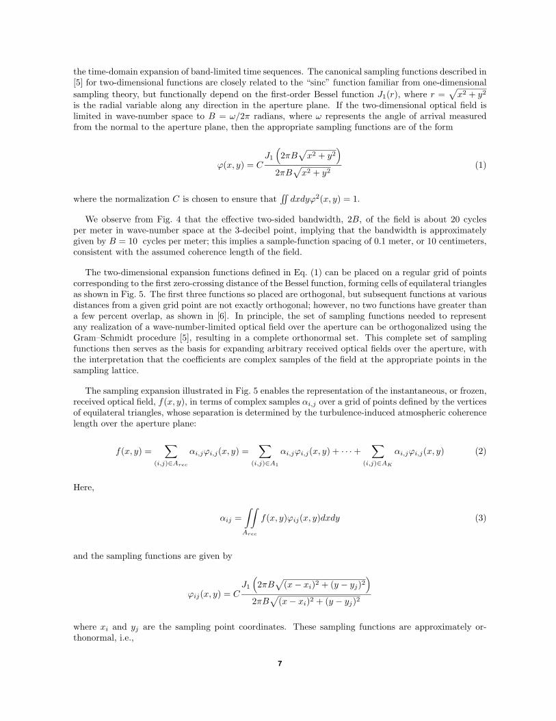
the time-domain expansion of band-limited time sequences. The canonical sampling functions described in[5] for two-dimensional functions are closely related to the “sinc” function familiar from one-dimensionalsampling theory, but functionally depend on the first-order Bessel function J1(r), where r =

√x2 + y2

is the radial variable along any direction in the aperture plane. If the two-dimensional optical field islimited in wave-number space to B = ω/2π radians, where ω represents the angle of arrival measuredfrom the normal to the aperture plane, then the appropriate sampling functions are of the form

ϕ(x, y) = CJ1

(2πB

√x2 + y2

)2πB

√x2 + y2

(1)

where the normalization C is chosen to ensure that∫∫

dxdyϕ2(x, y) = 1.

We observe from Fig. 4 that the effective two-sided bandwidth, 2B, of the field is about 20 cyclesper meter in wave-number space at the 3-decibel point, implying that the bandwidth is approximatelygiven by B = 10 cycles per meter; this implies a sample-function spacing of 0.1 meter, or 10 centimeters,consistent with the assumed coherence length of the field.

The two-dimensional expansion functions defined in Eq. (1) can be placed on a regular grid of pointscorresponding to the first zero-crossing distance of the Bessel function, forming cells of equilateral trianglesas shown in Fig. 5. The first three functions so placed are orthogonal, but subsequent functions at variousdistances from a given grid point are not exactly orthogonal; however, no two functions have greater thana few percent overlap, as shown in [6]. In principle, the set of sampling functions needed to representany realization of a wave-number-limited optical field over the aperture can be orthogonalized using theGram–Schmidt procedure [5], resulting in a complete orthonormal set. This complete set of samplingfunctions then serves as the basis for expanding arbitrary received optical fields over the aperture, withthe interpretation that the coefficients are complex samples of the field at the appropriate points in thesampling lattice.

The sampling expansion illustrated in Fig. 5 enables the representation of the instantaneous, or frozen,received optical field, f(x, y), in terms of complex samples αi,j over a grid of points defined by the verticesof equilateral triangles, whose separation is determined by the turbulence-induced atmospheric coherencelength over the aperture plane:

f(x, y) =∑

(i,j)∈Arec

αi,jϕi,j(x, y) =∑

(i,j)∈A1

αi,jϕi,j(x, y) + · · · +∑

(i,j)∈AK

αi,jϕi,j(x, y) (2)

Here,

αij =∫∫Arec

f(x, y)ϕij(x, y)dxdy (3)

and the sampling functions are given by

ϕij(x, y) = CJ1

(2πB

√(x − xi)2 + (y − yj)2

)2πB

√(x − xi)2 + (y − yj)2

where xi and yj are the sampling point coordinates. These sampling functions are approximately or-thonormal, i.e.,

7

⟨

⟨

⟨

⟨

⟨

⟨

⟨⟨

Arec

A2

A1

Fig. 5. Sampling grid over the receiver aperture definingplacement of sampling functions and illustrating the interpre-tation of the field as samples over the entire aperture and overtwo subapertures.

r0

∫∫Arec

ϕ2ij(x, y)dxdy ≈ 1

and

∫∫Arec

ϕij(x, y)ϕkl(x, y)dxdy ≈ 0, i = k, j = l

As shown in Fig. 5, the coefficients αij represent samples of the field over the (i, j)th grid point. Due tothe circular symmetry and unimodal nature of the two-dimensional sampling functions defined in Eq. (1),these samples may be interpreted as effective coherent areas of radius r0 centered over each grid pointshown by the dashed circle in Fig. 5. Note that we have not taken into account boundary conditions at theedge of the aperture; nor have we formally applied the Gram–Schmidt procedure to fully orthogonalizethe basis functions. Therefore, this representation is somewhat approximate but is sufficiently accurateto motivate the development of optical array receiver theory starting with a single large aperture.

If we take the magnitude squared of the complex received field and integrate it spatially over the entireaperture, we obtain the power of the signal field through the aperture. Applying this operation to bothsides of Eq. (2) yields

∫∫Arec

dxdy∣∣f(x, y)

∣∣2 =∫∫

Ared

dxdy

∣∣∣∣∣∣∑

(i,j)∈Arec

αijϕij(x, y)

∣∣∣∣∣∣2

∼=∑

(i,j)∈Arec

∣∣αij

∣∣2 (4)

where the last expression follows from the approximate orthonormality of the sampling functions. Sincethe left side of Eq. (4) represents the total power of the signal, so does the right-hand side, with theinterpretation that the signal power over the receiver aperture can be built up from the sum of the

8

individual sample powers. Equivalently, the total power through the aperture can be viewed as the sumof powers collected by small effective apertures centered over each grid point. Note that if the fieldcoherence length is equal to or greater than the diameter of the receiver aperture, then a single samplingfunction suffices to represent the field: in this case, there is only one coefficient in the expansion, andthe total signal power through the aperture equals the squared magnitude of the sample representing theentire received optical field.

Summarizing the key features of the array model, we conclude the following:

(1) The amount of background power collected by any diffraction-limited receiver aperture isa constant independent of the aperture dimensions, because the diffraction-limited fieldof view (steradians) is inversely related to the receiver area.

(2) The amount of coherent signal power collected by a diffraction-limited receiver is directlyproportional to the collecting area. For the case of free-space (not turbulent) reception,the signal is in the form of a plane wave that represents a uniform power density in unitsof power per unit area; for the turbulent case, the plane wave is broken up into smallcoherence areas over the collecting aperture, but the total average signal power collectedby the receiver remains the same.

Based on the above model, the following general conclusion follows:

(3) A necessary condition to ensure that total signal and noise powers collected by an arrayof subapertures is of the same total area as a single large receiver is that each subaperturecontain at least one sampling coefficient.

This conclusion follows from the interpretation of the sample coefficients as small coherence areassurrounding the center of each sampling function, with effectively constant (complex) value throughout.This model effectively replaces the continuous field model with a discrete representation, where now thetotal power through the aperture is the sum of the squares of the coefficients. In effect, we have replacedintegration over a continuous area with a sum of discrete terms, where each coefficient represents powerflowing through a small area over the aperture; these equivalent areas are disjoint and cover the entireaperture. Subapertures containing more than one sample of the field can be constructed in a similarmanner, as shown in Fig. 5, conserving energy since the total power flowing through a given subaperturecan be estimated by counting the number of discrete signal-field samples it contains.

Whereas the signal energy per sample collected by a coherence area can be estimated directly from thecoefficients, the background power cannot, since it is not coherent over the same area as the turbulence-degraded signal field; the background energy is more easily estimated from the conventional plane-wave de-composition illustrated in Fig. 2. However, since the total background power collected by any diffraction-limited receiver is the same, it follows that each coherence area represented by an aperture-plane samplecollects P ∗

b microwatts of background power. Therefore, according to this model, the total signal powercollected by a subaperture containing K samples is proportional to

∑Kk=1 |αk|2, whereas the total back-

ground power is proportional to K P ∗b . This conclusion is correct for any subaperture containing at least

one sample, from the smallest area with diameter equal to a coherence length to the largest single-aperturereceiver containing a great many coherence areas. We conclude that, as long as each subaperture containsat least one signal sample, the total amount of signal and background energy can be built up from theprimitive coherence-area samples, and therefore a single large aperture can be constructed as the sum ofnon-overlapping subapertures with an equivalent collecting area. This model holds over any region onthe ground where the turbulence parameters are constant, typically on the order of hundreds of meters ormore, and hence over areas much greater than any single-aperture receiver under consideration. There-fore, the centers of the subapertures can be separated by relatively large distances, creating an arrayfrom the single large aperture receiver, without affecting the collected signal power and the collected

9

background power. Arrays of receivers therefore are equivalent to a single-aperture receiver of the samecollecting area in the sense that both collect the same total signal and background power, as asserted inconclusion (3), stated above.

However, these conclusions do not extend to the case where the diameters of the array elements becomesmaller than the atmospheric coherence length. The reason is that, as the coherence area is subdividedinto smaller apertures while holding the total area constant, creating in effect subsample apertures, thesignal power flowing through each subsample aperture remains proportional to the subsample area, thusconserving signal power, but the background noise power flowing into each subsample aperture is a con-stant independent of collecting area. This means that each subsample aperture collects less signal powerwhile collecting the same background power; therefore, receiver performance suffers. Alternatively, thetotal signal power collected by a full-sample aperture and the equivalent array of subsample aperturesremains constant as the number of array elements increases, but the total noise power increases propor-tionally with the number of array elements. A direct consequence of this behavior is the observation thatin the absence of turbulence, so that the field coherence length is equal to or greater than the collectingarea, subdividing the single aperture into subapertures results in degraded performance when backgroundnoise is present. This, of course, is merely a restatement of the fact that coherence areas cannot be sub-divided without collecting more noise power than signal power and so incurring a performance loss. Wemay conclude, therefore, that single-aperture receivers of any diameter can be subdivided into arrays ofsmaller apertures only if the number of array elements remains smaller than the number of signal samplesneeded to represent the signal field over the receiver aperture. The above concepts can be restated interms of the largest single receiver aperture diameter, D, and atmospheric coherence length, r0:

(4) The performance of an array of small telescopes is equivalent to that of a single-aperturereceiver of the same collecting area and diameter, D, provided the number of arrayelements, N = KL (K detector elements per telescope, L telescopes), obeys the conditionN ≤ (D/r0)2 ≡ N∗.

Since the only cause of performance degradation is background radiation, it follows that in the absenceof background radiation the total number of array elements, N , is not constrained to be less than N∗.Therefore, in situations where the background radiation is not significant—such as might be the case atnight with appropriate narrowband optical filtering—any number of elements could be used to constructan array without suffering performance degradation. However, as a practical matter, the constraint onthe number of array elements is not a serious impediment to array design, as the following exampleillustrates.

Example. It is generally accepted that even under the best possible seeing conditions on the ground,the Fried parameter typically does not exceed 20 centimeters at an operating wavelength of 1 micrometerduring the day. If a 10-meter aperture is needed to communicate from deep space, then the maximumnumber of elements permissible for an array receiver is N ≤ (D/r0)2 = (10/0.2)2 = 2500. This numberis far greater than what is needed to synthesize a 10-meter aperture with reasonably sized telescopes; infact, with 1-meter apertures, only 100 telescopes would be needed.

We may conclude from this example that, since turbulence is always present during ground reception,an array of telescopes can be constructed with a reasonable number of elements to synthesize a singlelarge-aperture receiver for communications applications.

IV. Array Receiver Performance

In the following analyses, we shall assume that the optical bandwidth of the receiver is great comparedto its electrical bandwidth, so that a multimode assumption can be applied to both the signal andbackground fields. It has been shown that multimode Gaussian fields with suitably small average modalnoise count generate approximately Poisson-distributed random-point processes at the output of an ideal

10

photon-counting detector [2]. This model is reasonable for communications systems operating even atgigabit-per-second rates, and justifies the use of the relatively simple Poisson model which, in turn, oftenleads to mathematically tractable solutions.

A. Array Detector Model

Consider an array of detectors consisting of K×L detector elements, representing K detector elementsper telescope (FPA) and L telescopes. Assuming a frozen-atmosphere model, the sample-function densityof the array of count observables from a particular focal-plane detector element of a given telescope can bewritten as p[Nmn(t)|λmn(t); 0 ≤ t < T ], where λmn(t) and Nmn(t) represent the Poisson count intensityand number of counts, respectively, over the mnth detector element, and where m indexes a detectorelement in the focal plane of the nth telescope [2]. This represents the output of a particular elementof the array. Note that if the spatial intensity distribution is known, and the location and size of eachdetector element are also known, then conditioning on the spatial intensity distribution is equivalent toconditioning on the array of intensity components, each of which is still a function of time. Assumingthat each detector element observes the sum of a signal field plus multimode Gaussian noise field, thearray outputs can be modeled as conditionally independent Poisson processes, conditioned on the averagesignal intensity over each detector element. The joint conditional sample-function density over the entirearray can be expressed in terms of the KL dimensional vector N(t) as

p[N(t)|λ(t); 0 ≤ t ≤ T

]=

K∏m=1

L∏n=1

p[Nmn(t)|λmn(t); 0 ≤ t < T

](5)

where N(t) ≡(N11(t), N12(t), · · · , NKL(t)

). This detection model can be used as a starting point for prob-

lems involving hypothesis testing and parameter estimation, where the desired information is containedin the intensity distribution but only the array of count accumulator functions can be observed.

B. Hypothesis Testing with Poisson Processes

Consider M -ary pulse-position modulation (PPM) in which one of M intensity functions is received,and the receiver attempts to determine the correct symbol based on observations of the array of countaccumulator functions over each of M time slots. It is assumed that the symbol boundaries are knownand that the arrival time of each detected photon and the total number of detected photons can be storedfor a limited duration of time necessary for processing.

With M -ary PPM modulation, a signal pulse of duration τ seconds is transmitted in one of M con-secutive time slots, resulting in a PPM symbol of duration T = τM seconds. As shown in [2], thelog-likelihood function can be expressed as

Λi(T ) =K∑

m=1

L∑n=1

∑wj,mn∈((i−1)τ,iτ ]

ln(

1 +λs,mn(wj,mn)

λb

)

=K∑

m=1

L∑n=1

ln(

1 +λs,mn

λb

)N (i)

mn (6)

where wj,mn is the occurrence time of the jth photon over the mnth detector element within the ithtime slot, N

(i)mn is defined as the total number of photons occurring over the mth detector element in

the focal plane of the nth telescope during the ith time slot, λs,mn is the count intensity due to signalover the mnth detector element, and λb is the count intensity due to background noise. Note that with

11

constant signal intensities the actual arrival times of photons within each slot do not contribute to thedecision, hence only the total number of detected photons, N

(i)mn, matters. Given that we know the

intensity over each detector element, the ith log-likelihood function consists of the sum of a logarithmicfunction of the ratio of signal and background intensities from all detector elements over the ith pulseinterval, multiplied by the total number of detected photons; the optimum detection strategy is to selectthe symbol corresponding to the greatest log-likelihood function.

C. Performance of the Optimum Detector-Array Receiver

The probability of a correct decision is the probability that the log-likelihood function associated withthe transmitted symbol exceeds all other log-likelihood functions. Thus, when the qth symbol is sent,then a correct decision is made if Λq(T ) > Λi(T ) for all i = q. Denoting the logarithmic functions, orweights, in Eq. (6) by u

(i)mn, the log-likelihood function can be rewritten as

Λi(T ) =K∑

m=1

L∑n=1

u(i)mnNmn (7)

In this form, we can see that the log-likelihood function is composed of sums of a random numberof weights from each detector element; for example, the mth detector element in the nth telescopecontributes an integer number of its own weight to the sum. Note that detectors containing much morebackground than signal intensity do not contribute significantly to the error probability, since the outputsof these detector elements are multiplied by weights that are close to zero. This observation suggests thefollowing suboptimum decoder concept with greatly simplified structure: list the detector elements fromall telescopes simultaneously, starting with the one containing the most signal energy, followed by everyother detector ordered according to decreasing signal intensities. In effect, the logarithmic weights arepartitioned into two classes: large weights are assigned the value one, while small weights are assignedthe value zero. It was shown previously that this simple partitioning achieves near-optimum performancein low- to moderate-background environments, but with greatly reduced decoder complexity.

The processing to determine which detector elements to use from the array to achieve best perfor-mance can be explained as follows: compute the probability of error for the first detector element plusbackground, then form the sum of signal energies from the first two detector elements (plus backgroundfor two detector elements), and so on, until the minimum error probability is reached. The set of detectorelements over all telescopes that minimizes the probability of error for the entire array is selected, as thisset achieves best performance. However, this straightforward process of performing the optimization isnot practical for an array of telescopes, since the output of each detector element must be sent to a centralprocessing assembly, where the computations are performed; while this is conceptually straightforward,the complexity required to achieve this processing with a large number of wideband channels quicklybecomes prohibitive.

For the adaptively synthesized array detector, the probability of correct decision given hypothesis q, orHq, can be obtained by assuming constant signal and background intensities over each time slot, yieldingthe conditional Poisson densities

pq(k|Hq) =(λsτ + λbτ)k

k!e−(λsτ+λbτ) (8a)

and

pi(k|Hq) =(λbτ)k

k!e−λbτ (8b)

12

Here we interpret λsτ as the total average signal count per PPM slot over the selected set of detectorelements when a signal is present, and λbτ as the total average background count over the same set ofdetector elements, per PPM slot. As shown in [2], the probability of correct symbol decision is given by

PM (C) =

M−1∑r=0

(1

r + 1

) (M − 1

r

) ∞∑k=1

(λsτ + λbτ)k

k!e−(λsτ+λbτ)

[(λbτ)k

k!e−λbτ

]rk−1∑

j=0

(λbτ)j

j!e−λbτ

M−1−r

+ M−1e−(λs+Mλb)τ (9)

and the probability of symbol error follows as PM (E) = 1 − PM (C).

Performance of the array receiver was evaluated via simulated phase disturbances over each telescopeof the array, using Kolmogorov phase screens as described in [7]. A sample field was generated usingthe distorted phase distribution, resulting in a matrix of complex signal amplitudes over each aperture.For these simulations, an atmospheric correlation length of r0 = 10 centimeters was assumed. Thefield intensity generated in the detector plane of each telescope was integrated over the elements of a128× 128 pixel detector array, which is assumed to encompass the extent of the signal distribution in thefocal plane of each telescope.

The performance of an entire sequence of arrays, starting with one large element representing thesingle-element receiver implementation and subdividing it into 4, 16, and 64 smaller elements of constanttotal collecting area, was evaluated in the following manner. Error probability was computed for both idealturbulence-free conditions and for turbulence characterized by Fried parameter (or coherence length) ofr0 = 10 centimeters and an outer scale of turbulence corresponding to 64 meters. In a typical computation,the 128 × 128 = 16, 384 pixel energies representing the output of a single 4-meter aperture were sortedin decreasing order of average signal energy, and M -ary PPM symbol-error probabilities were calculatedfor increasing numbers of detectors, starting with the first detector. Let Ks denote the average numberof signal photons per PPM slot collected by the entire array aperture when a signal is present, and let kb

denote the average number of background photons per PPM slot collected by a diffraction-limited detectorelement (generally made up from several contiguous pixels). We also define the total average number ofbackground photons collected by the entire array aperture as Kb = (D/r0)2kb, where D is the diameter ofthe large single-aperture receiver. However, we should keep in mind that the adaptively synthesized focal-plane detector array typically rejects most of the background radiation, collecting background photonsselectively from those detector elements that contain significant signal energy. Figure 6 shows the symbol-error probability for 16-dimensional PPM (M = 16) as a function of the number of detector elementsused, for the case Ks = 10 photons per slot and kb = 0.01 photon per slot per diffraction-limited FOVor, equivalently, Kb = 4. It can be seen that for this case the smallest error probability of 10−2.7 ≈ 0.002is achieved by assigning unity weight to the first 50 pixels containing the greatest signal intensities andzero to all the rest.

The same approach was used to determine array receiver performance in the presence turbulence, asshown in Fig. 7. However, in this case the minimum-error probability is obtained with 1200 pixels sortedaccording to signal energy, instead of 50 as for the diffraction-limited case. In the presence of noise, thismeans that performance suffers, because 1200 pixels collect approximately 24 times as much backgroundnoise as the 50 sorted pixels that attained the minimum-error probability in the absence of turbulence.

13

0.0

−0.5

−1.0

−1.5

−2.0

−3.00 200 400 600 800 1000

pixels

log 1

0 P

M (

E )

Fig. 6. Probability of error as a function of the number of sortedpixels: no turbulence.

4 APERTURES, 1-m diameterNO TURBULENCEM = 16, Ks = 10, Kb = 4

−2.5

log 1

0 P

M (

E )

0.0

−0.2

−0.4

−0.6

−0.8

−1.0

−1.40 500 1000 1500 2000 2500 3000

pixels

Fig. 7. Probability of error as a function of the number of sortedpixels: moderate turbulence, r0 = 10 cm.

−1.2

4 APERTURES, 1-m diameterMODERATE TURBULENCEM = 16, Ks = 10, Kb = 4

14

The performance of the optical arrays was evaluated using the procedure described above to determinethe error probability of the adaptive “1-0” receiver. Arrays of various sizes, consisting of increasingnumbers of telescopes with proportionally smaller apertures to keep the total collecting area constant,were evaluated. Independent samples of Kolmogorov phase screens were generated for each telescope, andthe signal intensity distributions in the focal plane were determined for each sample function, using two-dimensional Fourier transforms. The focal plane of each telescope was assumed to contain a focal-planearray, of dimensions consistent with the telescope diameter and the expected level of turbulence.

In a typical simulation, a large telescope is analyzed first, by determining its performance accordingto the sorting procedure described above. The probability of error is calculated for increasing amountsof signal energy passing through the aperture, and distributed in the focal plane according to the two-dimensional Fourier transform of the aperture-field distribution generated using the Kolmogorov phase-screen program. Next, the diameter of each telescope was divided by two, generating four smaller tele-scopes with the same total area as the previous array, and the performance of the new larger array wascomputed as before. The process of dividing telescope diameters by a factor of two in order to generatethe next larger array was continued four times, generating arrays of 4, 16, and 64 elements from a singlelarge telescope. Different realizations of the signal intensity distribution were generated for each elementof the new array; thus, a single telescope used a single phase-screen realization over the aperture plane,whereas an array of N ×N telescopes of the same area as the single telescope used a total of N2 differentphase-screen realizations. The intensity distributions were then scaled such that the total signal energyentering the single large-aperture receiver and the array were equal.

An example of the phase distributions generated for analyzing array performance is shown in Figs. 8(a)and 8(b). The variation of optical phase over each telescope, when operating in turbulence with a Friedparameter of r0 = 0.1 meter (or 10 centimeters) and an outer scale of turbulence of 64 meters, is shown in

Fig. 8. A single 1-m-diameter telescope, 10-cm atmospheric-coherencelength: (a) aperture-plane phase distribution and (b) corresponding focal-plane intensity distribution .

80

60

40

6040

200

80

8060

4020

0

100

500

0

10050

0

150

050

100150

(a)

(b)

1-mRECEIVERAPERTURE

FOCAL-PLANEINTENSITYDISTRIBUTION

15

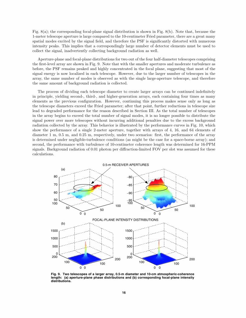
Fig. 8(a); the corresponding focal-plane signal distribution is shown in Fig. 8(b). Note that, because the1-meter telescope aperture is large compared to the 10-centimeter Fried parameter, there are a great manyspatial modes excited by the signal field, and therefore the PSF is significantly distorted with numerousintensity peaks. This implies that a correspondingly large number of detector elements must be used tocollect the signal, inadvertently collecting background radiation as well.

Aperture-plane and focal-plane distributions for two out of the four half-diameter telescopes comprisingthe first-level array are shown in Fig. 9. Note that with the smaller apertures and moderate turbulence asbefore, the PSF remains peaked and highly concentrated in the focal plane, suggesting that most of thesignal energy is now localized in each telescope. However, due to the larger number of telescopes in thearray, the same number of modes is observed as with the single large-aperture telescope, and thereforethe same amount of background radiation is collected.

The process of dividing each telescope diameter to create larger arrays can be continued indefinitelyin principle, yielding second-, third-, and higher-generation arrays, each containing four times as manyelements as the previous configuration. However, continuing this process makes sense only as long asthe telescope diameters exceed the Fried parameter; after that point, further reductions in telescope sizelead to degraded performance for the reason described in Section III. As the total number of telescopesin the array begins to exceed the total number of signal modes, it is no longer possible to distribute thesignal power over more telescopes without incurring additional penalties due to the excess backgroundradiation collected by the array. This behavior is illustrated by the performance curves in Fig. 10, whichshow the performance of a single 2-meter aperture, together with arrays of 4, 16, and 64 elements ofdiameter 1 m, 0.5 m, and 0.25 m, respectively, under two scenarios: first, the performance of the arrayis determined under negligible-turbulence conditions (as might be the case for a space-borne array); andsecond, the performance with turbulence of 10-centimeter coherence length was determined for 16-PPMsignals. Background radiation of 0.01 photon per diffraction-limited FOV per slot was assumed for thesecalculations.

FOCAL-PLANE INTENSITY DISTRIBUTIONS

1500

(b)

1000

500

0200

100

0 0100

200

1500

1000

500

0200

100

0 0100

200

80

(a)0.5-m RECEIVER APERTURES

70

60

50100

50

0 050

100

−80

−85

−90

−95100

50

0 050

100

Fig. 9. Two telescopes of a larger array, 0.5-m diameter and 10-cm atmospheric-coherencelength: (a) aperture-plane phase distributions and (b) corresponding focal-plane intensitydistributions.

16

log 1

0 P

M (

E )

0

−1

−2

−4

−5

−6

−70 10 15 20

AVERAGE NUMBER OF SIGNAL PHOTONS, Ks

Fig. 10. Performance of a single 2-m telescope and an equivalent-aperture array receiver,with and without turbulence.

TURBULENCE, 10-cm COHERENCE LENGTH

−3

NO TURBULENCE

TELESCOPE DIAMETER: 2 mERROR PROBABILITY PM (E ):Kb = 4, r 0 = 10 cm, M = 16

0.25 m

0.5 m

1 mPHOTON-COUNTING

Figure 10 shows that with little or no turbulence, such that ro > D, the single large receiver performsbest. However, with significant turbulence, ro << D, the array performance is comparable to that of asingle large receiver.

Note that in the absence of turbulence a single large-aperture receiver performs best because the signalis in the form of an undistorted plane wave, and therefore a single detector element with diffraction-limitedFOV suffices to collect essentially all of the signal energy. At the same time, background radiation enteringthe receiver from all directions within the FOV can be maximally suppressed, only the minimal amountwithin the small diffraction-limited cone of angles contributing to background interference within the re-ceiver. Since diffraction-limited FOV and collecting area are inversely related, the amount of backgroundradiation in a diffraction-limited FOV is independent of receiver aperture; this means that N diffraction-limited receivers collect N times as much background energy as a single receiver, regardless of telescopediameter. Therefore, arrays of diffraction-limited receivers collect background energy proportional to thenumber of elements, not proportional to the total collecting area. The performance of diffraction-limitedarrays observing a signal in the absence of turbulence but with moderate background radiation in thediffraction-limited FOV of each telescope is illustrated in Fig. 10; note that performance degrades signifi-cantly as the number of array elements increases from a single 2-meter-diameter telescope to 4 telescopesof 1-meter aperture, then to 16, and finally to 64 telescopes of 0.25-meter diameter.

However, turbulence is ever present; even in good seeing (corresponding to a Fried parameter of10 centimeters or more), the performance of the first-generation array (of 4 telescopes) is virtually in-distinguishable from the performance of the single aperture, as the performance curves correspondingto turbulent conditions indicate. This occurs because in the presence of turbulence the single telescopemust increase its FOV well beyond the diffraction limit to collect sufficient signal energy to minimize theprobability of symbol error, and in the process collects more background energy as well. In effect, thesingle-aperture receiver must observe more than one (typically, a great many) spatial modes, each modeapproximated by a diffraction-limited FOV collecting both signal and background energy from slightlydifferent directions. The array of small telescopes observes the same total number of spatial modes, andhence collects the same amount of background energy by the above argument. Since the total collecting

17

area of the array is the same as that of the single receiver, it also collects the same amount of signalenergy; therefore, the performance of the array is essentially the same as that of the single-aperturereceiver. Small variations in the array performance curves with turbulence are due to slight variations ofthe random phase distributions generated by the Kolmogorov phase-screen program.

D. Extrapolating to Determine the Performance of Large Arrays

In order to determine if there is a “best” array telescope diameter, array performance was evaluatedfor a given value of total signal energy, background intensity, and turbulence parameter for a largenumber of arrays. As originally developed, computations for array performance can be carried out in areasonable amount of time (approximately 1 hour per run) for arrays of no more than 64 elements. Thisallows analysis of arrays consisting of up to 4 different telescope sizes (for example, 2 meter, 1 meter,0.5 meter, and 0.25 meter). It was found that increasing the array size beyond 64 elements, with eacharray containing its own focal-plane array of detectors, began to incur unacceptably great computationalburdens. Therefore, an approach was developed to evaluate the performance of a large array by modifyingthe input noise parameters of smaller arrays, and then “connecting” the results in order to estimateperformance over a much larger range of array diameters.

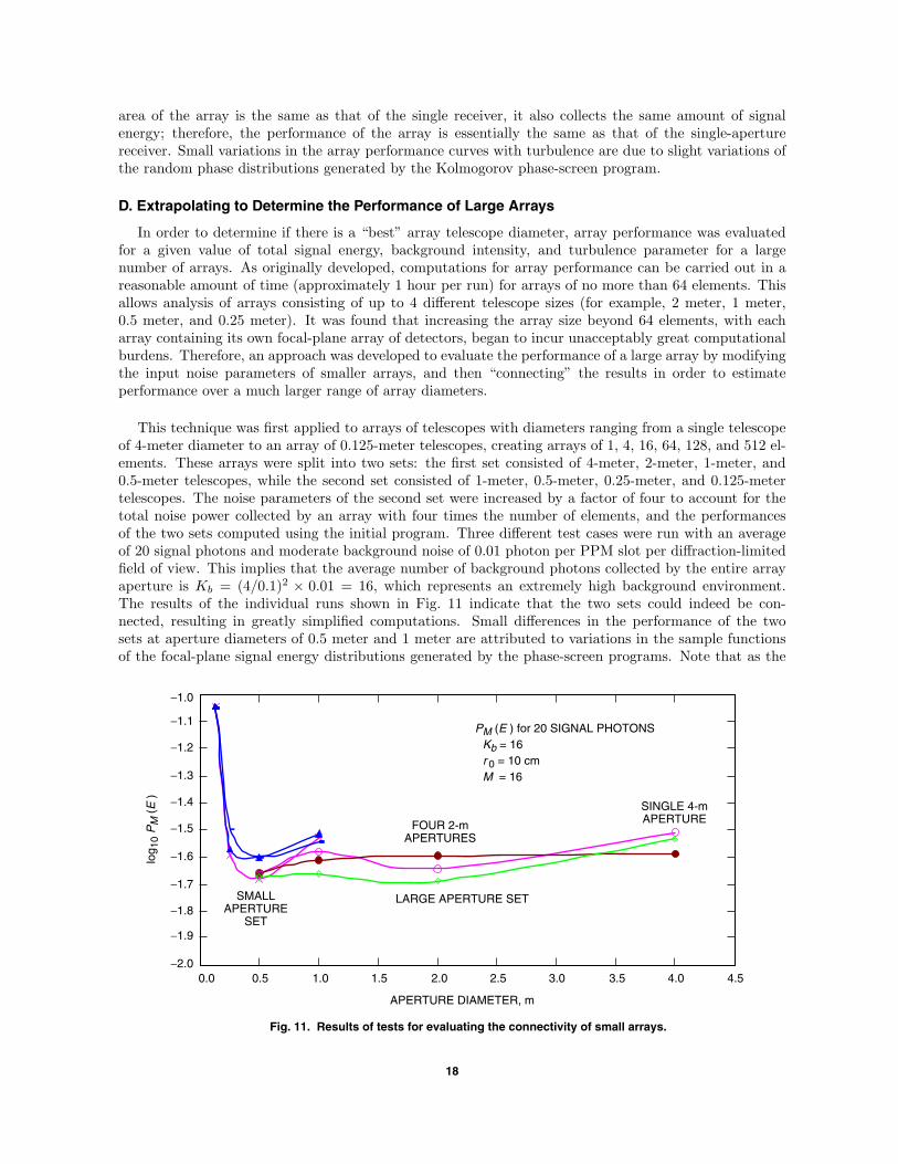
This technique was first applied to arrays of telescopes with diameters ranging from a single telescopeof 4-meter diameter to an array of 0.125-meter telescopes, creating arrays of 1, 4, 16, 64, 128, and 512 el-ements. These arrays were split into two sets: the first set consisted of 4-meter, 2-meter, 1-meter, and0.5-meter telescopes, while the second set consisted of 1-meter, 0.5-meter, 0.25-meter, and 0.125-metertelescopes. The noise parameters of the second set were increased by a factor of four to account for thetotal noise power collected by an array with four times the number of elements, and the performancesof the two sets computed using the initial program. Three different test cases were run with an averageof 20 signal photons and moderate background noise of 0.01 photon per PPM slot per diffraction-limitedfield of view. This implies that the average number of background photons collected by the entire arrayaperture is Kb = (4/0.1)2 × 0.01 = 16, which represents an extremely high background environment.The results of the individual runs shown in Fig. 11 indicate that the two sets could indeed be con-nected, resulting in greatly simplified computations. Small differences in the performance of the twosets at aperture diameters of 0.5 meter and 1 meter are attributed to variations in the sample functionsof the focal-plane signal energy distributions generated by the phase-screen programs. Note that as the

log 1

0 P

M (

E )

−1.1

−1.2

0.0 0.5 4.5

APERTURE DIAMETER, m

Fig. 11. Results of tests for evaluating the connectivity of small arrays.

PM (E ) for 20 SIGNAL PHOTONS

−1.0

Kb = 16r 0 = 10 cmM = 16−1.3

−1.4

−1.5

−1.6

−1.7

−1.8

−1.9

−2.01.0 1.5 2.0 2.5 3.0 3.5 4.0

FOUR 2-mAPERTURES

SINGLE 4-mAPERTURE

SMALLAPERTURE

SET

LARGE APERTURE SET

18

telescope diameters approach the Fried parameter performance deteriorates in all cases. The modalanalysis presented in Section III predicted this performance degradation for apertures smaller than thecoherence length; however, it is actually observed for somewhat larger collecting areas in Fig. 11. Thisbehavior is attributed to the fact that the modal analysis was only approximate, and did not take intoaccount edge effects that start to become significant under these conditions.

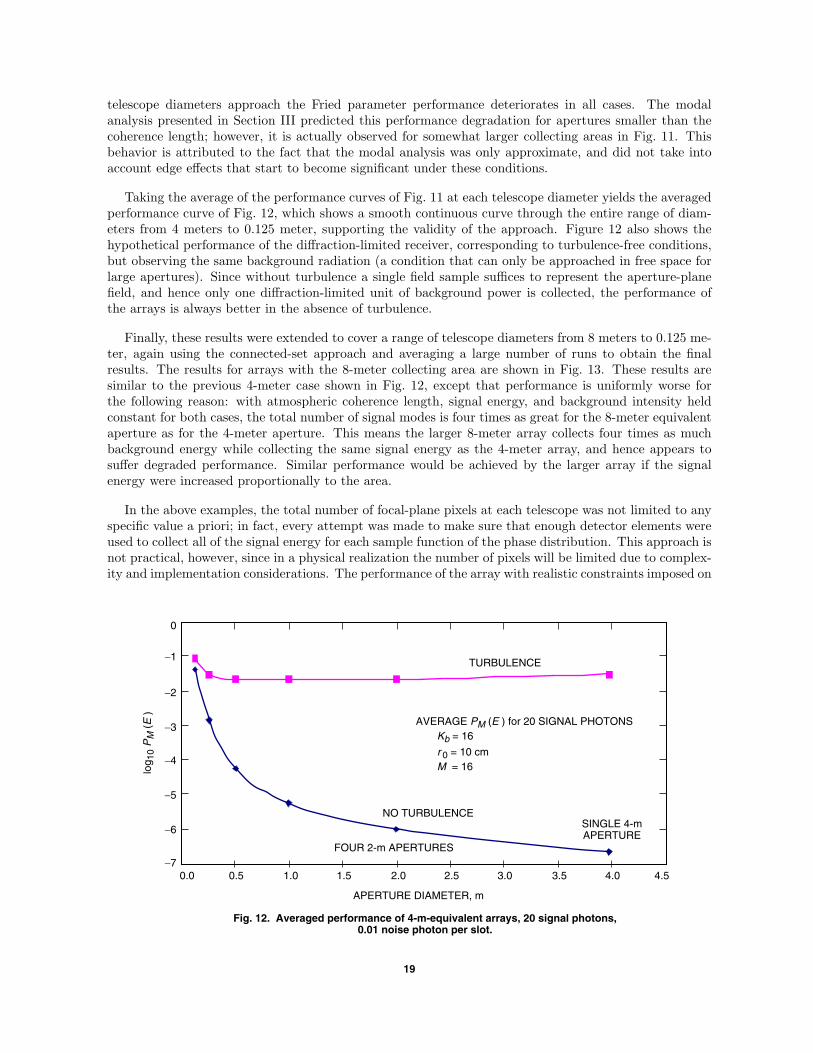
Taking the average of the performance curves of Fig. 11 at each telescope diameter yields the averagedperformance curve of Fig. 12, which shows a smooth continuous curve through the entire range of diam-eters from 4 meters to 0.125 meter, supporting the validity of the approach. Figure 12 also shows thehypothetical performance of the diffraction-limited receiver, corresponding to turbulence-free conditions,but observing the same background radiation (a condition that can only be approached in free space forlarge apertures). Since without turbulence a single field sample suffices to represent the aperture-planefield, and hence only one diffraction-limited unit of background power is collected, the performance ofthe arrays is always better in the absence of turbulence.

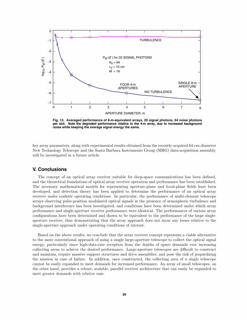
Finally, these results were extended to cover a range of telescope diameters from 8 meters to 0.125 me-ter, again using the connected-set approach and averaging a large number of runs to obtain the finalresults. The results for arrays with the 8-meter collecting area are shown in Fig. 13. These results aresimilar to the previous 4-meter case shown in Fig. 12, except that performance is uniformly worse forthe following reason: with atmospheric coherence length, signal energy, and background intensity heldconstant for both cases, the total number of signal modes is four times as great for the 8-meter equivalentaperture as for the 4-meter aperture. This means the larger 8-meter array collects four times as muchbackground energy while collecting the same signal energy as the 4-meter array, and hence appears tosuffer degraded performance. Similar performance would be achieved by the larger array if the signalenergy were increased proportionally to the area.

In the above examples, the total number of focal-plane pixels at each telescope was not limited to anyspecific value a priori; in fact, every attempt was made to make sure that enough detector elements wereused to collect all of the signal energy for each sample function of the phase distribution. This approach isnot practical, however, since in a physical realization the number of pixels will be limited due to complex-ity and implementation considerations. The performance of the array with realistic constraints imposed on

log 1

0 P

M (

E )

−1

−2

0.0 0.5 4.5

APERTURE DIAMETER, m

Fig. 12. Averaged performance of 4-m-equivalent arrays, 20 signal photons,0.01 noise photon per slot.

0

−3

−4

−5

−6

−71.0 1.5 2.0 2.5 3.0 3.5 4.0

TURBULENCE

NO TURBULENCE

AVERAGE PM (E ) for 20 SIGNAL PHOTONSKb = 16

r 0 = 10 cmM = 16

FOUR 2-m APERTURES

SINGLE 4-mAPERTURE

19

log 1

0 P

M (

E )

−1

−2

0 1 8

APERTURE DIAMETER, m

Fig. 13. Averaged performance of 8-m-equivalent arrays, 20 signal photons, 64 noise photonsper slot. Note the degraded performance relative to the 4-m array, due to increased backgroundnoise while keeping the average signal energy the same.

0

−3

−4

−5

−6

−72 3 4 5 6 7

TURBULENCE

NO TURBULENCE

PM (E ) for 20 SIGNAL PHOTONS

Kb = 64r 0 = 10 cmM = 16

FOUR 4-mAPERTURES

SINGLE 8-mAPERTURE

key array parameters, along with experimental results obtained from the recently acquired 64-cm-diameterNew Technology Telescope and the Santa Barbara Instruments Group (SBIG) data-acquisition assembly,will be investigated in a future article.

V. Conclusions

The concept of an optical array receiver suitable for deep-space communications has been defined,and the theoretical foundations of optical array receiver operation and performance has been established.The necessary mathematical models for representing aperture-plane and focal-plane fields have beendeveloped, and detection theory has been applied to determine the performance of an optical arrayreceiver under realistic operating conditions. In particular, the performance of multi-element telescopearrays observing pulse-position modulated optical signals in the presence of atmospheric turbulence andbackground interference has been investigated, and conditions have been determined under which arrayperformance and single-aperture receiver performance were identical. The performances of various arrayconfigurations have been determined and shown to be equivalent to the performance of the large single-aperture receiver, thus demonstrating that the array approach does not incur any losses relative to thesingle-aperture approach under operating conditions of interest.

Based on the above results, we conclude that the array receiver concept represents a viable alternativeto the more conventional approach of using a single large-aperture telescope to collect the optical signalenergy, particularly since high-data-rate reception from the depths of space demands ever increasingcollecting areas to achieve the desired performance. Large-aperture telescopes are difficult to constructand maintain, require massive support structures and drive assemblies, and pose the risk of jeopardizingthe mission in case of failure. In addition, once constructed, the collecting area of a single telescopecannot be easily expanded to meet demands for increased performance. An array of small telescopes, onthe other hand, provides a robust, scalable, parallel receiver architecture that can easily be expanded tomeet greater demands with relative ease.

20

References

[1] R. Gagliardi and S. Karp, Optical Communications, New York: John Wiley andSons, 1976.

[2] V. Vilnrotter and M. Srinivasan, “Adaptive Detector Arrays for Optical Com-munications Receivers,” IEEE Transactions on Communications, vol. 50, no. 7,pp. 1091–1097, July 2002.

[3] W. Pratt, Laser Communications Systems, New York: John Wiley and Sons,1969.

[4] J. W. Goodman, Introduction to Fourier Optics, New York: McGraw-Hill, 1968.

[5] D. Petersen and D. Middleton, “Sampling and Reconstruction of Wave-Number-Limited Functions in N-Dimensional Euclidian Spaces,” Information and Con-trol, vol. 5, pp. 279–323, 1962.

[6] V. Vilnrotter, Focal-Plane Processing for Scattered Optical Fields, Ph.D. Disser-tation, University of Southern California, June 1978.

[7] P. Negrete-Regagnon, “Practical Aspects of Image Recovery by Means of theBispectrum,” Journal of the Optical Society of America, vol. 13, no. 7, pp. 1557–1576, July 1996.

21