AN OVERLAPPED GROUP ITERATIVE METHOD FOR SOLVING LINEAR SYSTEMS Jos´ e M. Bioucas-Dias Instituto Superior T´ ecnico Instituto de Telecomunica¸ c˜ oes Torre Norte, Piso 10 Av. Rovisco Pais, 1049-001 Lisboa Email: [email protected]2001 Abstract We propose a new iterative method for the numerical computation of the solution of linear systems of equations. The method is suited to problems exhibiting local dependencies, such as those result- ing from the discretization of partial differential equations or from Markov random fields in image processing. The technique can be envisaged as a generalization of the Gauss-Seidel point iterative method being able, however, to achieve greater convergence rates. On each iteration, a group of variables is treated as unknown while the others are assumed known; the equations associated to the mentioned group are then solved in order to the unknown variables. The following iterations do the same, choosing other groups of variables. The successive groups overlap one another, departing definitely from the group iterative perspective, since in the latter case groups are disjoint. The over- lapped group (OG) method, herein introduced, is shown to converge for two classes of problems: (1) symmetric positive definite systems; (2) systems in which any principal submatrix is nonsingular and whose inverse matrix elements are null above (below) some upper (lower) diagonal. In class (2) the exact solution is reached in just one step. A set of experiments comparing OG convergence rate and computational complexity with those of other popular iterative methods, illustrates the effectiveness of the proposed scheme. 1
We propose a new iterative method for the numerical computation of the solution of linear systems
of equations. The method is suited to problems exhibiting local dependencies, such as those result-
ing from the discretization of partial differential equations or from Markov random fields in image
processing. The technique can be envisaged as a generalization of the Gauss-Seidel point iterative
method being able, however, to achieve greater convergence rates. On each iteration, a group of
variables is treated as unknown while the others are assumed known; the equations associated to
the mentioned group are then solved in order to the unknown variables. The following iterations do
the same, choosing other groups of variables. The successive groups overlap one another, departing
definitely from the group iterative perspective, since in the latter case groups are disjoint. The over-
lapped group (OG) method, herein introduced, is shown to converge for two classes of problems: (1)
symmetric positive definite systems; (2) systems in which any principal submatrix is nonsingular and
whose inverse matrix elements are null above (below) some upper (lower) diagonal. In class (2) the
exact solution is reached in just one step. A set of experiments comparing OG convergence rate and
computational complexity with those of other popular iterative methods, illustrates the effectiveness
of the proposed scheme.
1
1 Introduction
The need for solving N × N symmetric positive definite (SPD) linear systems
Ax = b, x ∈ RN , and A = AT , (1)
arises in several applications, namely in the solution of integral and partial differential equations,
image processing, time series analysis, statistics, control theory, etc. The algorithms for finding the
solution x∗ = A−1b can be classified as direct or iterative [1], [2], [3], [4].
1.1 Direct Methods
Direct methods, by definition, reach the exact solution within a finite number of operations. For
matrices without any special structure, the complexity of direct methods is O(N3), meaning that the
number of floating point operations1 is of the order of N3. When the system is large, a complexity
of is O(N3) unbearable. There are, however, classes of systems to which there exits faster direct
algorithms. A relevant example is the Toeplitz systems which can be solved with the Levinson
recursion formula [5], [6], [4] with O(N2) complexity, or with the algorithms proposed in [7], [8] with
complexity O(N ln2 N). If, besides Toeplitz, A is generated by a rational function of order (p, q),
methods proposed in [9], [10], and [11] have max(p, q) O(N) complexity.
The conjugate gradient (CG) method, introduced in [12], is another direct2 method for solving
SPD linear systems. The convergence rate of the CG method is determined by the spectrum pattern
of matrix A [13]. Roughly, it converges faster if the eigenvalues of A are clustered. The class
of preconditioned conjugate gradient (PCG) methods introduces a preconditioning step through a
matrix P on the CG method. From the spectral clustering point of view it is the matrix P−1A that
matters. The preconditioner P should be, somehow, close to matrix A. Preconditioners for Toeplitz
systems are studied in [14], [15], and [16]. A common feature to all these preconditioners is that
they can be easily inverted (by means of fast transforms such as the fast Fourier transform, cosine
transform, or sine transform), leading to superfast algorithms with complexity O(N ln N). Another
advantage of the PCG methods is that they can be parallelized, whenever the transform used can
be parallelized. Parallelization leads to a complexity O(log N), when N processors are used. For
non-Toeplitz matrices, there is no general approach concerning the conditioner design.
1Real additions and real multiplications.2The CG method is a direct method because it finds the solution after no more than N iterations. However, it
can also be classified as an iterative method, since it generally needs less than n iterations to achieve a solution with
acceptable precision. This is more evident in large systems.
2
1.2 Iterative Methods
Linear systems resulting from many signal and specially image problems are very large. A usual
feature of such huge systems is that the involved matrices are sparse; the interactions between
variables are usually confined to a small neighborhood. This can be found, for example, in linear
systems resulting from discretization of partial differential equations, where the interaction length
depends on the order of the highest derivative [1]. Also, in the field of image restoration, using
regularization principles or stochastic paradigms such as Markov random fields, the neighborhood
order is, frequently, much smaller than the line and column sizes [17], [18], [19]. Assuming Toeplitz
systems, the PCG method can still be applied. However, even for matrices with sparse structure, the
PCG method still leads to the same O(N ln N) complexity, since the inverse of a sparse matrix is not,
necessarily, sparse. Thus, the preconditioning step of PCG methods has still O(N ln N) complexity.
For large systems, iterative methods are preferred to direct methods [2]; despite the infinite time
they generally need to find the exact solution, they often yield a solution within acceptable error
with fewer operations than direct methods. Moreover, round off errors3 (or any other error), are
dumped out as the process evolves [2], [1], [20], [21].
For a wide class of sparse matrices (e.g. systems resulting from discretization of partial differential
equations or systems resulting from Gauss-Markov descriptions in signal and image processing), the
iteration complexity is O(N). Consequently, if an acceptable solution is reached in t0 iterations, with
t0 independent of N , then the overall complexity is still O(N). Another important and sometimes
determinant attribute of iterative methods is the mild storage requisites normally needed in the case
of sparse matrices.
Among iterative techniques, the Jacobi (J), the Gauss-Seidel (GS), and the successive overrelax-
ation (SOR) are well known and widely used methods. They belong to the class of linear stationary
iterative methods of first degree [1], [3]. They are also classified as point iterative, since each iteration
can be implemented by solving simple equations for each system component.
Group iterative methods [1] resemble point iterative ones, replacing each individual component by
a group, such that each component belongs to one and only one group [1]. If the groups form a
partitioning of the set S = {1, · · · , N}, the resulting method is known as a block method [20], [22].
Each of the above referred point methods has a correspondent block method; namely, the block
Jacobi (BJ), the block Gauss-Seidel (BGS), and the block successive overrelaxation (BSOR).
Block iterative methods were developed with the purpose of increasing the convergence rate of the
3For large and/or ill-conditioned systems, rounding errors due to floating-point arithmetic are, frequently, the main
problem of direct methods. Rounding errors can severely degrade the solutions found.
3
respective point methods. Assuming that A is a M -matrix, the BJ and BGS converge at least as
rapidly as the respective point counterparts [1]. On the other hand, if A is Stieltjes and π-consistently
ordered, then the BSOR method, implemented with the optimum relaxation factor, converges faster
than the SOR [1], [3]. It should be stressed that determining the exact (or approximate) relaxation
factor, necessary to the SOR and the BSOR methods, frequently has such a high cost that the
method is impracticable. A remarkable exception occurs whenever A has the socalled property A
[1], [3]. In this case it is possible to establish a relation between the eigenvalues of A (equivalently
the eginvalues of Jacobi iteration matrix) and the optimum relaxation factor. This procedure is very
effective, for example, in problems resulting from the discretization of elliptic differential equations
[1], [23].
1.3 Rationale of the Proposed Iterative Method
A shortcoming of the block methods, at least for those systems describing local interactions, is that
the error of each component tends to be larger on the block boundaries than on its interior4 This
pattern of behavior is illustrated in Fig. 4: the curve BSG-8 shows the error after the first iteration
of the BSG method with blocks of size 8. Notice the larger errors at the block boundaries. We will
back in more detail to this experiment in Section 5
The overlapped group (OG) iterative method, herein introduced, operates (as group methods do)
on groups of components. However, contrary to block methods, in the OG scheme groups are not
disjoint. By overlapping the groups in a proper manner, the distance between the components being
updated and the ones already updated is kept constant (or above a minimum positive number D).
Thus, by choosing the updated components with smaller error, it is expectable that the proposed
method converges faster than the block methods.
The OG method is a descent procedure that can be interpreted in terms of the evolution of the
quadratic function
F (x) =1
2xT Ax − bT x. (2)
If A is symmetric and positive definite, then F (x) is strictly convex; therefore, it has a unique
minimum x∗, satisfying ∇F (x∗) = Ax∗ − b = 0. Minimizing F (x) or solving the system Ax = b
are equivalent problems. In the i-th OG iteration, function F (x) is minimized with respect to the
components xj for j ∈ Si, where Si is a set of indices, keeping the components xk for k /∈ Si constant.
Iteration (i + 1) resembles the i-th one, replacing the set Si by Si+1 which partially overlaps the
former. The overlapping of sets Si is crucial concerning the achievement of larger convergence rates.
4Block boundaries depend on the problem and on the way that indexes are assigned to each site.
4
This behavior is illustrated by curves BSG-8 and OG-8 in Fig. 4: both methods use blocks of size 8;
however the blocks in OG-8 have an overlaping of 7, whereas in BSG-8 they do not overlap. Notice
the smaller error of OG-8 after the first iteration.
On the other hand, a suitable implementation of the proposed strategy demands, approximately,
the same computational burden as the Gauss-Seidel (which corresponds to the choice Si = {i})applied on the original system.
According to the rationale just presented, it is expectable that the sequence {x(n)} produced by
the OG method converges to x∗ = A−1b, whenever A is a SPD matrix; this result is shown in Section
4. Besides SPD systems, convergence is also studied for systems whose inverse matrix elements are
null above (below) some upper (lower) diagonal. For these matrices, there are choices of the sets Si
such that the OG method takes only one iteration to converge.
The paper is organized as follows. Section 2 introduces the OG method formally. A comparison with
the multisplitting methods and a reinterpretation under the light of the multigrid concept is also
provided. Section 3 proposes a filter-like implementation, makes considerations about complexity,
and shows that there exists an equivalent system from the Gauss-Seidel iteration point of view.
Section 4 presents convergence results. Section 5 shows results of a series of experiments and makes
comparisons with other iterative methods. Section 6 ends the paper by presenting some concluding
remarks. The proofs of the theorems on convergence are given in the Appendix.
2 Overlapped Group Method
The first step to implement the OG method is the definition of the iteration groups5:
Definition 1 An ordered covering g of S = {1, . . . , N} is an ordered collection of subsets Si ⊂ S,
with i = 1, . . . , ng such that ∪i=ng
i=1 Si = S. Two ordered coverings g and g′ given by S1, . . . , Sng and
S ′1, . . . , S
′n′
g, respectively, are identical if ng = n′
g and if S1 = S ′1,. . .,Sng = S ′
n′g.
Definition 1 differs from an ordered grouping [1], in that sets Si in the latter are necessarily disjoint.
A one-dimensional (1D) oriented covering is g1(D) ≡ {S1, . . . , SN−D+1}, where
Si = {i, i + 1, . . . , i + D − 1}, i = 1, . . . , N − D + 1. (3)
The Covering (3) is suited to system matrices with its significant elements close to the main diagonal.
This is quite often the picture in 1D processing problems.
5The designation of group is not to be understood in the usual mathematical sense.
5
• • • • • • • • • • • • • • • •
• • • • • • • • • • • • • • • •
• • • • • • • • • • • • • • • •
• • • • • • • • • • • • • • • •
• • • • • • • • • • • • • • • •
• • • • • • • • • • • • • • • •
• • • • • • • • • • • • • • • •
• • • • • • • • • • • • • • • •
• • • • • • • • • • • • • • • •
1 2 … j N2
…
1 2
…
i
…
N1
Sij
Future of (i,j)
Past of (i,j)
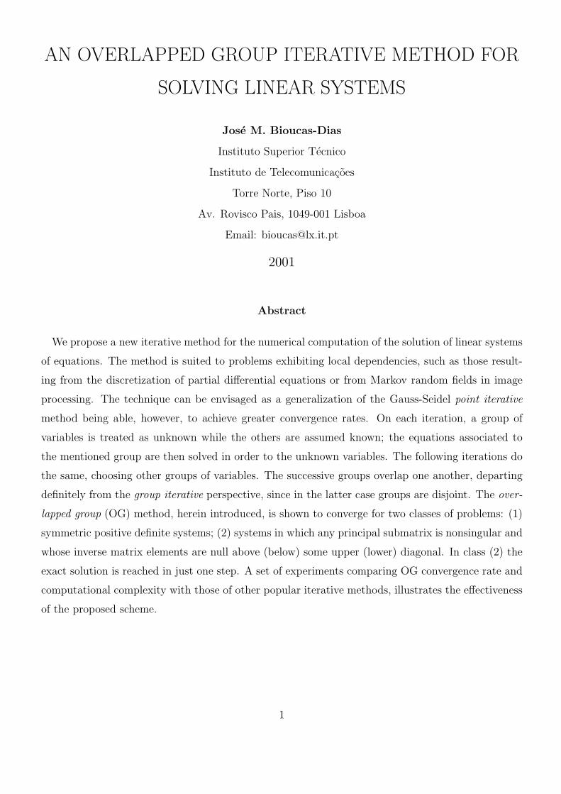
Figure 1: Illustration of a set Sij which is an element of the 2D oriented covering g2(2, 2). The
regions named past and future denote those sites (k, l) ∈ L such that (k, l) < (i, j), and (k, l) ≥ (i, j),
respectively.
Two-dimensional (2D) problems are frequently defined on regular lattices of the form L = {(i, j)| 1 ≤i ≤ N1, 1 ≤ j ≤ N2}. Using the order relation on L induced by the lexicographic ordering (by row),
a 2D oriented covering is g2(D1, D2) ≡ {Si,j, i = 1, . . . , N1 − D1 + 1 j = 1, . . . , N2 − D2 + 1}, where
We now introduce the subsequence x(n = t ng), with t ∈ N (the set of naturals), which is the
output of OG iteration after t full sweeps of index i in (5). The index t in x(t) and the index n in
x(n) will distinguish both sequences6 . Using this notation, equation (10) becomes
x(t) = Mx(t − 1) + Nb t = 1, 2, . . . (13)
which is a linear stationary iterative method of first degree [1]. Solving the recursion (13), one is led
to
x(t) = M tx(0) +i=t−1∑i=0
M iNb. (14)
If N−1 exists, then, the sequence {x(t)} is generated by the splitting A = B − C, with B = N−1,
and C = N−1M .
Assume that matrix M is convergent (i.e., its spectral radius satisfies ρ(M) < 1). This implies
that (see [1])
x∞ = limt→∞
x(t) =
(∞∑i=0
M i
)Nb = (I − M)−1Nb. (15)
Defining e(t) = x(t) − x∞, and after some manipulation involving (13) and (15), one is led to
e(t) = M te(0). (16)
Thus, if M is convergent, the distance between x(t) and x∞ decays geometrically. Conversely, if M is
not convergent, there exist starting points x(0), for which the recursion (13) diverges [1]. Of course,
the only interesting case is x∞ = x∗ = A−1b. In Section 4, two classes of systems exhibiting the
latter property are studied.
6This notation is of course incorrect since we are naming different functions with basis on their arguments. We
have adopted it however for the sake of lightness of the exposition.
8
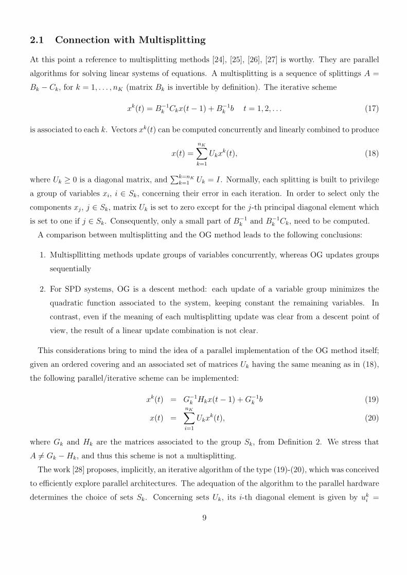
2.1 Connection with Multisplitting
At this point a reference to multisplitting methods [24], [25], [26], [27] is worthy. They are parallel
algorithms for solving linear systems of equations. A multisplitting is a sequence of splittings A =
Bk − Ck, for k = 1, . . . , nK (matrix Bk is invertible by definition). The iterative scheme
xk(t) = B−1k Ckx(t − 1) + B−1
k b t = 1, 2, . . . (17)
is associated to each k. Vectors xk(t) can be computed concurrently and linearly combined to produce
x(t) =
nK∑k=1
Ukxk(t), (18)
where Uk ≥ 0 is a diagonal matrix, and∑k=nK
k=1 Uk = I. Normally, each splitting is built to privilege
a group of variables xi, i ∈ Sk, concerning their error in each iteration. In order to select only the
components xj, j ∈ Sk, matrix Uk is set to zero except for the j-th principal diagonal element which
is set to one if j ∈ Sk. Consequently, only a small part of B−1k and B−1
k Ck, need to be computed.
A comparison between multisplitting and the OG method leads to the following conclusions:
1. Multispllitting methods update groups of variables concurrently, whereas OG updates groups
sequentially
2. For SPD systems, OG is a descent method: each update of a variable group minimizes the
quadratic function associated to the system, keeping constant the remaining variables. In
contrast, even if the meaning of each multisplitting update was clear from a descent point of
view, the result of a linear update combination is not clear.
This considerations bring to mind the idea of a parallel implementation of the OG method itself;
given an ordered covering and an associated set of matrices Uk having the same meaning as in (18),
the following parallel/iterative scheme can be implemented:
xk(t) = G−1k Hkx(t − 1) + G−1
k b (19)
x(t) =
nK∑i=1
Ukxk(t), (20)
where Gk and Hk are the matrices associated to the group Sk, from Definition 2. We stress that
A = Gk − Hk, and thus this scheme is not a multisplitting.
The work [28] proposes, implicitly, an iterative algorithm of the type (19)-(20), which was conceived
to efficiently explore parallel architectures. The adequation of the algorithm to the parallel hardware
determines the choice of sets Sk. Concerning sets Uk, its i-th diagonal element is given by uki =
9
[∑ng
k=1 ISk(i)]−1. Thus, in the t-th iteration, the new variable value xj(t) is given by the mean of
xkj (t) for j ∈ Sk, and k = 1, . . . , ng. It should be stressed that the scheme proposed in [28] results
more from hardware adequation than from an intentional implementation of scheme (19)-(20).
Given an arbitrary starting vector x(0), the sequence {x(t)} generated by (19)-(20) is convergent
if and only if matrix
M =
ng∑k=1
UkG−1k Hk (21)
is convergent. It would be worthy to compare ρ(M) with ρ(MJ), where MJ = D−1A (LA + UA) is
the Jacobi iteration matrix, DA is the diagonal of A, and LA and UA are the negative strictly lower
and the negative strictly upper triangular parts of A, respectively. It would also be interesting to
compare convergence rates of matrix M with convergence rates of multisplitting schemes. However,
this is out of the scope of this work.
2.2 Connection with Multigrid
Let x∗ be the solution of Ax = b (by hypothesis A−1 exists). Frequently, x∗i depends on far data
variables bk: |k − i| ≫ 0. This fact penalizes the convergence rate of iterative methods, and fostered
the multigrid approach [29]. The underlying idea is that one should firstly determine the long
distance (low frequency) components of the solution, by means of some subsampling scheme, and
next determine the short distance (high frequency) components of the solution, by means of some
interpolation scheme. The OG method, under covering g1(D), produces a local inversion of size D.
In this way, the component xi(t + 1) receives information from data components bk up to distance
k = i + D − 1. Moreover, if x∗i depends only on bk: k < i + B (which is equivalent to having A−1
elements null above the upper B-th diagonal) and D ≥ B+1, then the OG method finds the solution
in one step (a proof of this result is given in section 4). Thus, the OG method embodies, in this
sense, the multigrid philosophy. A similar set of ideas applies equally to 2D-problems.
3 Implementation
Assuming segmentation g1(D) defined in (??) and D = 1, the OG method reduces to the GS
method. Otherwise (D > 1), if equation (5) was directly implemented, it would involve a complexity
per iteration greater than the GS scheme and even greater than block methods (considering blocks of
size D). However, it is possible to compute x(t) with fewer operations. This is going to be illustrated
for segmentation g1(D).
10
= A4
a41
a51
a61
a42
a52
a62
a43
a53
a63
a47
a57
a67
a48
a58
a68
a49
a59
a69
X4
a41
a51
a61
a42
a52
a62
a43
a53
a63
a47
a57
a67
a48
a58
a68
a49
a59
a69
A4 =
x1
x2
x3
x7
x8
x9
B4
b1
b2
b3
b7
b8
b9
x1
x2
x3
x7
x8
x9
b1
b2
b3
b7
b8
b9
X4 = B4 =
A41 A42 A43 A47 A48 A49
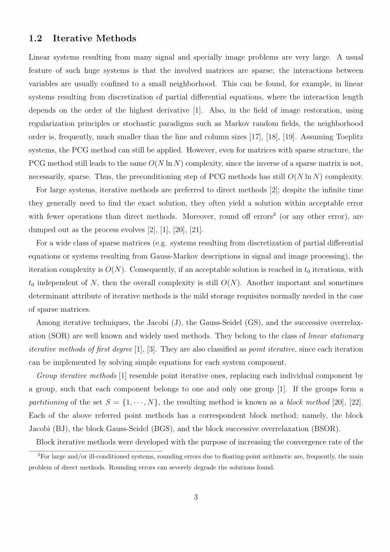
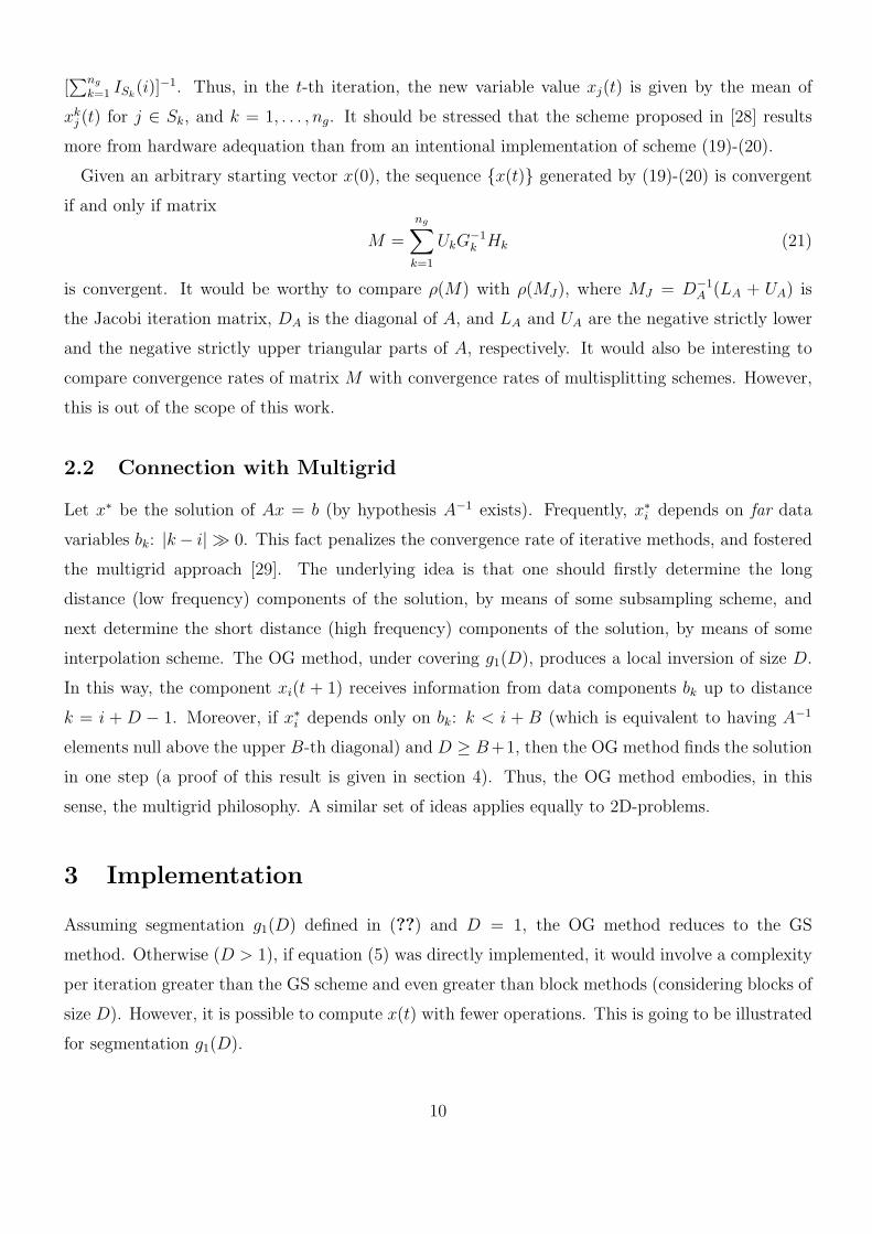
Figure 2: Schematization of submatrices introduced in Definition 3, for N = 9, D = 3, and S4 =
{4, 5, 6}.
Let A[Si|Sj], for Si, Sj ∈ g, denote the submatrix of A obtained by removing from A all lines and
columns whose indexes are not in Si and Sj, respectively. In the same fashion define b[Si] as the
subvector of column vector b obtained by removing from b all components whose indexes are not in
Si.
At this point it is convenient to introduce the following submatrixes:
Definition 3 Given the sets Si ∈ g and Si = Sci (complement of Si with respect to {1, 2, . . . , N}),
the matrix A, and the vectors b and x we introduce: Ai = A[Si|Si], Ai = A[Si|Si], Aij = A[Si|{j}],for j = 1, . . . , N , Xi = x[Si], X i = x[Si], Bi = b[Si], and Bi = x[bi].
Figure 2 depicts an instance of the entities above defined for segmentation g1(3), N = 9, and
S4 = {4, 5, 6}. Notice that matrices Ai and Ai are obtained from Qi and Qi by deleting their null
row and columns.
Consider the n-th iteration (5) such that i = saw(n, ng) and i + D ≤ N : although vector Xi
has dimension D, only its first component xi needs to be computed. This is so because: (1) the
components xj, j = i + 1, . . . , i + D − 1 will be updated in the next iteration; (2) the new values
of the variables in the group Si+1 depend on xj(t) for j = i + D + 1, . . . , N , and on xj(t + 1), for
j = 1, . . . , i. Thus, in the n-th iteration, only xi(t + 1) needs to be computed, being wasteful to
process the complete block. Only if i = N −D + 1, it becomes necessary to compute all components
of XN−D+1.
11
z -1 z -1 z -1
×
·
× × × ×
∑
× ×
· ·
·
− φ4(t)
s
as+1,s as+2,s as+3,i
p4 s p3
s p2 s p1
s
xi(t) xi(t-1)
φ4(t) s φ3(t)
s φ2(t) s φ1(t)
s
− −
−
+ xi(t)
xi(t-1)
φ3(t) 1 φ2(t)
1 φ1(t) 1
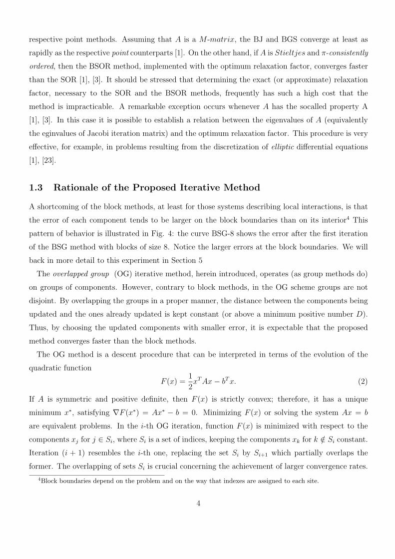
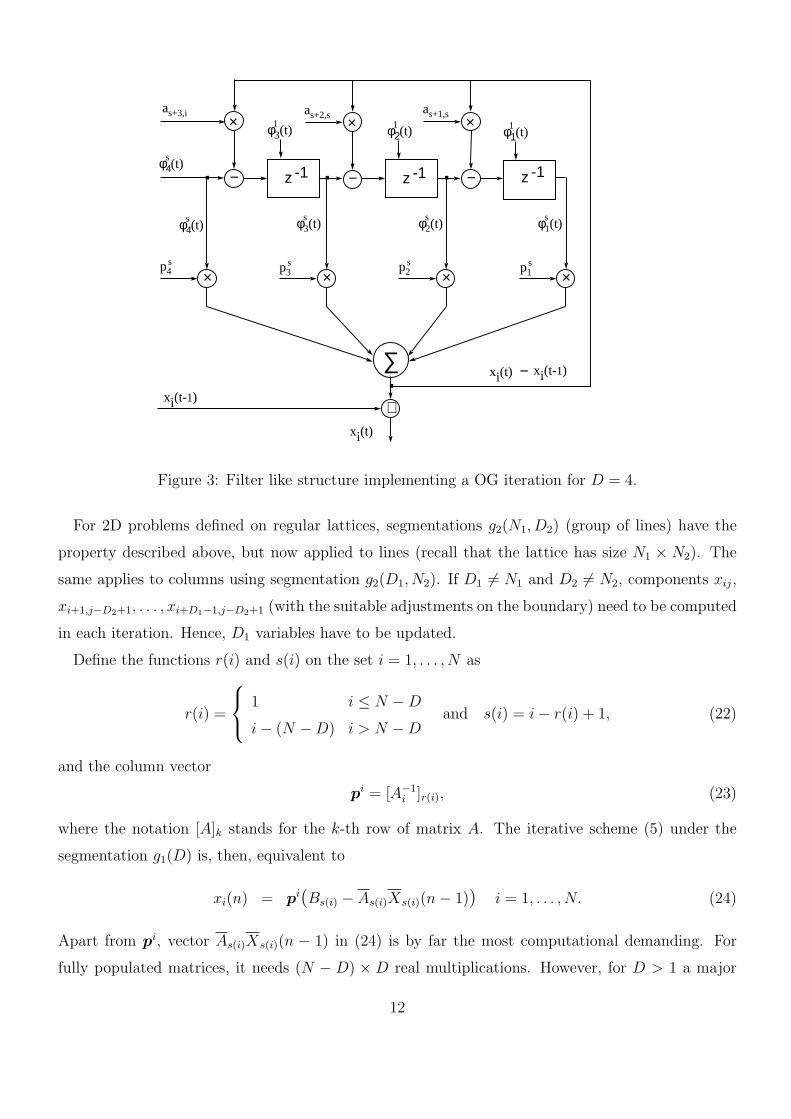
Figure 3: Filter like structure implementing a OG iteration for D = 4.
For 2D problems defined on regular lattices, segmentations g2(N1, D2) (group of lines) have the
property described above, but now applied to lines (recall that the lattice has size N1 × N2). The
same applies to columns using segmentation g2(D1, N2). If D1 = N1 and D2 = N2, components xij,
xi+1,j−D2+1, . . . , xi+D1−1,j−D2+1 (with the suitable adjustments on the boundary) need to be computed
in each iteration. Hence, D1 variables have to be updated.
Define the functions r(i) and s(i) on the set i = 1, . . . , N as
r(i) =
1 i ≤ N − D
i − (N − D) i > N − Dand s(i) = i − r(i) + 1, (22)
and the column vector
pi = [A−1i ]r(i), (23)
where the notation [A]k stands for the k-th row of matrix A. The iterative scheme (5) under the
segmentation g1(D) is, then, equivalent to
xi(n) = pi(Bs(i) − As(i)Xs(i)(n − 1)) i = 1, . . . , N. (24)
Apart from pi, vector As(i)Xs(i)(n − 1) in (24) is by far the most computational demanding. For
fully populated matrices, it needs (N − D) × D real multiplications. However, for D > 1 a major
12
component of (24) can be determined recursively. Noting that piAs(i) = [δ(k − r(i)), k = 1, . . . , D],
where δ is the kronecker symbol, one can write (recall that x(t) = x(n = t ng))
xi(t) = xi(t − 1) + piϕs(i)(t) with i = 1, . . . , N, (25)
with
ϕs(t) = Bs −k=s−1∑k=1
Ask xk(t) −k=N∑k=s
Ask xk(t − 1) s ≤ N − D + 1. (26)
The components of ϕs(t) = [ϕs1(t), . . . , ϕ
sD(t)]T satisfy
ϕs+1k (t) = ϕs
k+1(t) − a(s+k)s[xs(t) − xs(t − 1)] s ≤ N − D
ϕsD(t) = bs+D−1 −
k=s−1∑k=1
a(s+D−1)k xk(t) −k=N∑k=s
a(s+D−1)k xk(t − 1) s ≤ N − D + 1,(27)
for k = 1, . . . , D − 1. Fig. 3 depicts a filter-like structure implementing an iteration (s = s(i),
i = 1, . . . , N , ps = [ps1, . . . , p
sD], and t constant) described by equations (25) and (27). Terms
ϕ11(t), . . . , ϕ
D−11 (t) on top of the delay taps represents the initial values, and are given by (26).
The implementation herein proposed applies to the segmentation g1(D). For segmentations g2(N1, D2),
the same concepts and ideas still apply with the convenient adjustments (replacing each one-dimensional
element by N1-dimensional elements). However, for other segmentations with some degree of nonreg-
ularity, it is no longer possible to implement the OG method with equations (25) and (27). Indeed,
the lack of regularity implies that some (or a lot of) pairs Si, Si+1 do not overlap (or overlap irreg-
ularly) determining the computation of an irregular number of components of Xi(n); this leads to a
higher computational burden.
3.1 A Gauss-Seidel iteration point of view
Introducing definition (26) in equation (25), one obtains
xi(t) = xi(t − 1) +
(piBs(i) −
k=i−1∑k=1
piAs(i)k xk(t) −k=N∑k=i
piAs(i)k xk(t − 1)
), (28)
valid for i = 1, . . . , N and t = 1, 2, . . . Noting that piAs(i)i = 1, the iteration (28), can be rewritten
as
xi(t) =
(b′i −
k=i−1∑k=1
a′ik xk(t) −
k=N∑k=i+1
a′ik xk(t − 1)
), (29)
where b′i = piBs(i) i = 1, . . . , N
a′ik = piAs(i)k i, k = 1, . . . , N.
(30)
13
Equation (29) defines a GS iteration applied to the system A′x = b′, with A′ = TA, b′ = Tb, and
T =
p11 p1
2 · · · p1D 0 · · · · · · 0
0 p21 p2
2 · · · p2D 0 · · · 0
.... . . . . . . . . . . . . . . . . .
...
0 · · · 0 pN−D1 pN−D
2 · · · pN−DD 0
0 · · · · · · 0... · · · · · · ... A−1
N−D+1
0 · · · · · · 0
. (31)
If matrix T is nonsingular, systems Ax = b and A′x = b′ are equivalent. This happens if and only
if p11 = 0, · · · , pN−D
1 = 0 and A−1N−D+1 exists (in the next section this is shown to be true for PD
systems). Matrix A′ = TA has the following structure:
Proof 1 Proposition 1 is a immediate consequence of the geometric nature of the error e(t) and of
the properties of matrix norms. Q.E.D.
The OG algorithm has been introduced as a generalization of the GS method, able to achieve
greater convergence rates, while having, roughly, the same complexity. The main line of argument
is that the OG method is able to see D variables farther ahead, and use this information in order
to update the present variable in a more accurate fashion. However, this does not mean that the
convergence rate always increases as D increases. As in block methods [1], also OG method can
exhibit slower converge rates than the GS method. The following example confirms this fact: consider
the matrix A = BBT + C, with B = [exp(−|τ |)], C = [2(−1/2)|τ |] being Toeplitz. For N = 32,
the spectral radius7 ρ(MOG−D) is ρ(MOG−1) = 0.15677, and ρ(MOG−2) = 0.158342, i.e. ρ(MOG−2) >
ρ(MOG−1). Nevertheless, for D = 3, 4, 5, the spectral radius is ρ(MOG−3) = 0.00282, ρ(MOG−4) =
0.00122, and ρ(MOG−5) = 0.00014, respectively.
Choosing a covering is the first step towards the implementation of the OG method. We do not
know any expedite way to obtain a well suited covering for a given matrix. However, the following
result, shown in the Appendix, can help and give hints concerning this matter:
7Whenever the covering g1(D) is under assumption, we denote by MOG−D the respective iteration matrix. The
symbol MBGS−D denotes the BGS iteration matrix having blocks of size D. Iteration matrices of GS and SOR
methods are denoted by MGS and MSOR, respectively. Notice that MGS = MOG−1 = MBGS−1.
18
Theorem 2 Let Ax = b be a linear system, such that any principal submatrix of A in nonsingular.
Moreover, the elements of A−1 = [rij] verify rij = 0 for j − i ≥ B. Given the covering g1(D) such
that D ≥ B, the OG iteration matrix M is null.
This result gives credence to the rationale underlying the OG method sketched in Section 1. The
less xi depends on bi+k, for k > D, the faster the method converges to the true solution.
Theorem 2 considers matrices A−1 having zero elements in its upper right part. In the case of A−1
having zero elements in its lower left part (rij = 0 for j − i ≤ −D), then the OG method under the
covering
g1(D) : Si = {N − i + 1, . . . , N − i − D + 2}, i = 1, . . . , N − D + 1 (44)
finds the solution x∗ in one step. This is, of course, a minor modification of Theorem 2.
5 Numerical Results
This section presents four numerical examples comparing the OG method with other methods. Two
classes of system matrices A = [aij] are studied: (1) Toeplitz matrices; (2) quasi-regular matrices
(those with a high degree of regularity, except for a few elements).
covering g1(D) is used in all examples. We denote the convergence rate of method X ∈ {OG,GS, BGS, SOR}by R(X) = ln10(ρ(X)), where ρ(X) denotes the spectral radius of matrix MX . Whenever a block
method is being considered the letter D in X − D denotes the block size.
5.1 Toeplitz matrices
Example 1: aij = exp[−(
j−ia
)2].
Table 1 displays results for a =√
3 and N = 64 (for N = 128 the results are equal up to the
third digit). The condition number (given by κ(A) = σn(A)/σ1(A), where σn(A) and σ1(A) are the
largest and the smallest singular values of A, respectively) of matrix A, for a =√
3, is κ(A) ≃ 800,
accounting for an ill conditioned matrix.
Elements of A−1 = [rij] verify |rij/rii| ≪ 1, for |τ | = |j − i| > 10. Thus, the high convergence rate
of the OG method for D = 10 is essentially in accordance with Theorem 2, concerning one-sided
banded A−1 matrices. The superior performance of the OG method, compared with BGS, is evident
for D ≥ 1. Compared with the SOR method, the OG has much higher convergence rate for D ≥ 3.
Assume now that a = 1. Although smaller, spectral radii ρ(MGL−D), ρ(MBGS−D), and ρ(MSOR)
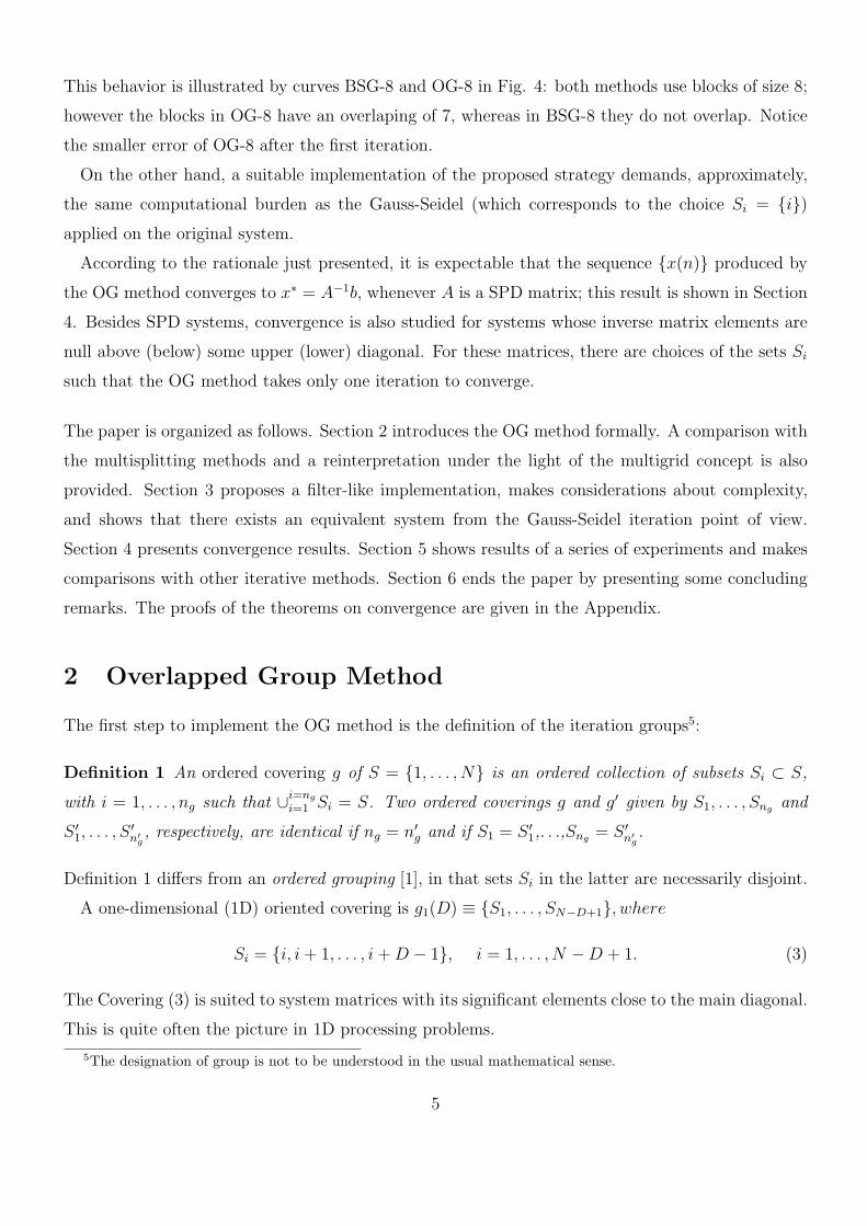
exhibit the same behavior evidenced by Table 1. Fig. 4 plots the error components |xi(1) − x∗i |, for
19
D ρ(MOG−D)R(OG)
R(GS)ρ(MBGS−D)
R(BGS)
R(GS)ρ(MSOR)
R(SOR)
R(GS)
GS≡ 1 0.99227 1 – – 0.93666 8.4
2 0.95354 6.13 0.97307 3.52 –
3 0.85930 19.54 – – –
4 0.71047 44.06 0.95525 5.90 –
5 0.53687 80.15 – – –
10 0.05264 379.42 0.92107 10.60 –
Table 1: Spectral radii and convergence ratios of Example1.
i-th component 1 8 16 24 32 40 48 56 64
100
|| xi (1) - x i ||2 / Ö N *
OG-8
BGS-8
10-1
10-2
10-3
10-4
10-5
Figure 4: Error components for OG and BGS methods, after the first iteration.
i = 1, · · · , 64, with b = 0, x(0) = [1, · · · , 1]T , and D = 8, after the first iteration, for the BGS and
the OG methods, respectively. The BGS method displays errors much larger tan the the OG error,
for any component. This was to be expected given the large magnitude of ρ(MBGS−8)/ρ(MOG−8) ≃(0.17)/(2.72 10−6). The BGS error exhibits a saw-type shape with maxima at i = 8, 16, 24, 32, 40, 48,
and 56, and minima at i = 1, 12, 20, 28, 36, 44, and 52. A crude justification8 is the following: the
error of each variable inside each block increases with the errors of variables outside the block and
decreases as the distance to the nearest boundary grows. In contrast, the OG method keeps the
distance to the variable with larger error at a constant value of 8; the exception is the last block, this
not being a problem (for both methods) if the variables in the last group do not depend on distant
groups.
The preconditioned conjugate gradient(PCG) method, in the case of Toeplitz systems, can be ap-
8This argument is valid for problems displaying local interactions.
20
plied with great success (PCG) [16]. Namely, if the matrix is generated by a rational sequence
(which is always the case of banded matrices), then the PCG complexity is O(N log N) [16], [31].
To be more precise, considering the preconditioner K1 proposed in [16], the PCG method takes
N(2(2B + 1) + 6 + 6 ln2 N) real additions and multiplications9 per iteration. The precondition-
ing step takes 4.5 N ln2 N addictions plus 1.5 N ln2 N multiplications. On the other hand, the OG
method (implemented by its GS equivalent) takes N(2(2B)) operations per iteration plus a neg-
ligible overhead necessary to compute A′ (recall that matrix A′ is quasi-Toeplitz) and b′. Thus,
if limN→∞ ρGS < 1, the OG method has, at least asymptotically, less complexity than the PCG
method. On the other hand, for a given N , it can happen that the OG method produces a solution
with acceptable error, with fewer operations than the PCG. This is illustrated in the next example.
Example 2: aij = (3/5)|j−i| + (−1/2)|j−i|, j − i ≤ 5 and aij = 0 for j − i ≥ 6.
D ρ(MGL−D)R(OG)
R(GS)ρ(MBGS−D)
R(BGS)
R(GS)ρ(MSOR)
R(SOR)
R(GS)
GS≡ 1 0.29837 1 – – 0.29197 1.018
2 0.27067 1.08 0.28569 1.04 –
3 0.02351 3.10 – – –
4 0.00855 3.93 0.18485 1.34 –
5 0.00822 3.97 – – –
10 0.00004 8.37 0.11790 1.77 –
Table 2: Convergence ratios for Example 2.
Results displayed in Table 2 were computed using N = 32. As a general remark, the convergence
rates exhibit the same pattern as the ones of Table 1. Again, we would like to recall the attention
to the spectral radius ρ(MOG−4) = 0.00855. The elements of matrix A−1 = [rij] satisfy |rij/rii| ≪ 1
if |j − i| ≥ 4. Thus, one can say that ρ(MGL−4) = 0.00855 is in accordance with Theorem 2. Fig.
5 plots the evolution of the Euclidian error ∥x(t) − x∗∥2 for GS, CG, OG, and PCG methods. The
horizontal axis is graduated with a scale representing the ratio between the the number of operations
per iteration Nop (of the different methods) and the number of operations per iteration of the OG
method. For N = 32, B = 5 and D = 4 that ratio takes the value 2.9. The number of operations
9The term 6N ln2 N account for the preconditioning step; term N(2(2B+1)) account for the matrix-vector product;
term 6N accounts the remaining vector-vector product. Notice that, in the case of banded matrices, its is better
compute directly matrix-vector products than embedding it in a circular convolution an using FFT techniques to do
it. Indeed, this last procedure would lead to a complexity O(N ln N) instead of the actual N(2(2B + 1)).
21
0 5 10 15 20 2530
-601. 10
-491. 10
-381. 10
-271. 10
-161. 10
0.00001
Nop
N[2(2B)]
||x(t) - x*||2
OG-4
GS
* • • • * * • *
• * • • *
*
* • •
* *
•
* *
• •
→
*
CG
PCG
0
Figure 5: Euclidian error of the OG, GS, CG, and PCG methods, for successive iterations.
per iteration, for the GS and OG methods, are taken to be equal. The same is done with CG and
PCG methods. Since the CG method takes N(4(2B +1))+6) operations per iteration, the true CG
convergence rate is even worse than the one plotted in Fig. 5 .
The PCG method finds the exact solution at 11-th iteration. This result is in accordance with
[16]: matrix A is generated by a rational sequence with (p = 5, q = 0). Thus, the spectrum of K−11 A
has at most 2 max(p, q) eigenvalues different from one, and, consequently, the solution is found, at
most, in 1+2 max(p, q) iterations. However, after the number of operations that PCG method needs
to reach the 11-th iteration, the OG method outputs a solution with an error smaller that 10−50.
We also ran this example with N = 128. The ratio ρ(MOG−4, N = 64)/ρ(MOG−4, N = 32) is 1.035.
On the other hand, PCG method still converges in 1 + 2 max(p, q) iterations; however, it now takes
3.5 times more operations than the OG method. This would allow an error attenuation better than
10−70 if the OG method was run with the same number of operations.
It should be stressed that, given a system with dimension N , the comparison between PCG and OG
method is not always as favorable to the latter. In fact, in order to achieve a competitive convergence
ratio, it might be necessary such a high D that applying the OG method is no longer effective.
5.2 Quasi-regular matrices
Typically, in restoration problems a degraded version (the observed signal/image) of the original
signal/image x is filtered in order to produce an estimate of the latter. Assuming that the data has
22
zero mean, is observed under a linear operator B, and is contaminated with independent Gaussian
zero mean noise, then, different approaches such as Wiener filtering [32], constrained least square
[17], Bayesian methods [17], the maximum entropy principle [32], or the regularization approach [17],
[18] demand the solution of the linear system Ax = b, where x is the estimate, b depends on the
observed data, and A is of the form
A = BBT + ηP. (45)
The meaning of η and P depends on the underlying paradigm. In the Bayesian framework matrix
P models the a priory knowledge, and η depends on the noise to signal ratio [17]. On the other
hand, in the regularization approach η is the regularization parameter and P is a matrix expressing
constraints on unknown vector x [18].
In the one-dimensional example we are about to present, P express the constraints on pairs of
components (xi, xi+1): either (xi+1, xi) is continuous (the difference xi+1 − xi must be small), or
(xi+1, xi) is discontinuous (the difference xi+1 − xi can take arbitrary values). The i-th row of P
express the continuity or discontinuity constraint as follows:
1. [. . . , 0,−1, 2,−1, 0, . . .], if components (xi−1, xi, xi+1 are continuous
2. [. . . , 0, 0, 1,−1, 0, . . .], if components (xi, xi+1) are continuous, and components (xi−1, xi) are
discontinuous
3. [. . . , 0,−1, 1, 0, 0, . . .], if components (xi, xi+1) are discontinuous, and components (xi−1, xi) are
continuous
4. [. . . , 0, 0, 0, 0, 0, . . .], if components (xi, xi+1) are (xi−1, xi) are discontinuous
Model (45) with P just presented is related with the weak string model [33]. This model aims
at the joint estimation of the discontinuities and the vector x. The exact solution, (carried out
by maximizing a proper objective function), is analytically and computationally very demanding.
Iterative algorithms achieving suboptimal solutions [33], [34], [35] have been proposed. A common
procedure to all this algorithms is that, in each iteration, they need to compute the inverse of a
matrix of the form (45). Matrix A is ill-conditioned for low signal to noise ratios, or ill-conditioned
matrices BBT , this leading to a high computational burden, concerning A−1 computation.
The following one-dimensional instance of (45) is going to be considered:
Example 3: B = [bij], with bij = exp[−( |j−i|a
)2] (Gaussian blur). We assume that discontinuities
occur at i = 9, 14, 16, 19, 20, 30, 31, and that a = 3 and η = 0.1.
23
D ρ(MGL−D)R(OG)
R(GS)ρ(MBGS−D)
R(BGS)
R(GS)ρ(MSOR)
R(SOR)
R(GS)
GS≡ 1 0.99043 1 – – 0.97815 2.30
2 0.87747 13.59 0.99167 0.87 – –
3 0.85908 15.80 – – – –
4 0.68044 40.04 0.98123 1.97 – –
5 0.63302 47.55 – – – –
10 0.16127 189.75 0.97884 2.22 – –
Table 3: Spectral radii and convergence ratios for Example 3.
For the present setting, the condition number of A is κ(A) = 1742.52, reflecting a severely ill
conditioned matrix. We call the attention for the very low converge rate of the GS method: R(GS) =
0.00417. Notice that, with this figures, an attenuation of 10−6 over the initial error would take,
approximately 1450 GS iterations. The ratio R(OG)/R(GS) for D = 4 is 40. Hence, the same
attenuation of 10−6 would take, approximately, 36 OG iterations. Gains of SOR and BGS methods
(even for D = 10) over GS are, by far, smaller than the OG ones.
By varying parameter η in (45) from zero to ∞ one can give more importance to BBT or, instead,
to P . Table 4 displays the ratio R(OG)/R(GS) for D = 4, a = 3, and η = 10i with i = −2, . . . , 2.
Table 5 displays the ratio R(OG)/R(GS) for D = 4, η = 0.1, and a = 10i with i = −1, 0, 1.
Results, displayed in Tables 4 and 5 have the same behavior: they grow monotonically with the
condition number κ(A). Thus, the more ill-conditioned the system matrix, the greater the OG
method convergence rate compared with that of the GS method.
(a = 3) η κ(A)R(OG)
R(GS)
10−2 8525.05 234.83
10−1 1742.52 40.04
100 512.83 10.58
101 305.16 8.87
102 1886.16 27.12
Table 4: Convergence ratios of Example 3, for a = 3, D = 4, and η variable.
Example 4: Similar to Example 3, but with N = 64 and the discontinuities occuring at sites
9, 14, 16, 19, 20, 30, 31, 41, 46, 48, 52, 53, 62, 63. Notice that for i ≥ 32, the string is broken at sites
displaced of a value 32 relative to Example 1.
24
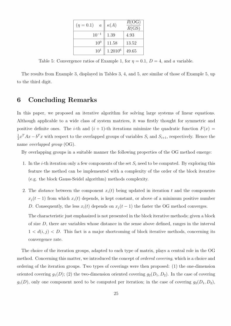
(η = 0.1) a κ(A)R(OG)
R(GS)
10−1 1.39 4.93
100 11.58 13.52
101 1.20106 49.65
Table 5: Convergence ratios of Example 1, for η = 0.1, D = 4, and a variable.
The results from Example 3, displayed in Tables 3, 4, and 5, are similar of those of Example 5, up
to the third digit.
6 Concluding Remarks
In this paper, we proposed an iterative algorithm for solving large systems of linear equations.
Although applicable to a wide class of system matrices, it was firstly thought for symmetric and
positive definite ones. The i-th and (i + 1)-th iterations minimize the quadratic function F (x) =
12xT Ax− bT x with respect to the overlapped groups of variables Si and Si+1, respectively. Hence the
name overlapped group (OG).
By overlapping groups in a suitable manner the following properties of the OG method emerge:
1. In the i-th iteration only a few components of the set Si need to be computed. By exploring this
feature the method can be implemented with a complexity of the order of the block iterative
(e.g. the block Gauss-Seidel algorithm) methods complexity.
2. The distance between the component xi(t) being updated in iteration t and the components
xj(t − 1) from which xi(t) depends, is kept constant, or above of a minimum positive number
D. Consequently, the less xi(t) depends on xj(t − 1) the faster the OG method converges.
The characteristic just emphasized is not presented in the block iterative methods; given a block
of size D, there are variables whose distance in the sense above defined, ranges in the interval
1 < d(i, j) < D. This fact is a major shortcoming of block iterative methods, concerning its
convergence rate.
The choice of the iteration groups, adapted to each type of matrix, plays a central role in the OG
method. Concerning this matter, we introduced the concept of ordered covering, which is a choice and
ordering of the iteration groups. Two types of coverings were then proposed: (1) the one-dimension
oriented covering g1(D); (2) the two-dimension oriented covering g2(D1, D2). In the case of covering
g1(D), only one component need to be computed per iteration; in the case of covering g2(D1, D2),
25
D2 components have to be computed per iteration. In 2D problems, if D1 has the size of a line, each
line can be treated as if it was a single component (the same is true for columns).
Assuming covering g1(D), two implementations were proposed: (1) based on the system Ax = b;
(2) based on a Gauss-Seidel equivalent system A′x = b′, with A′ = TA, b′ = Tb, and T being an
upper triangular D-banded matrix. The complexities of both implementations are of the same order;
the first is suited for high convergence rates, and the second for slow convergence rates. The analysis
of matrix A′ led to the conclusion that the OG method can be thought of as a balance between
recursiveness and iterativeness.
The product TA can also be viewed as preconditioning step on matrix A. Given that the OG
method preserves the number of non-null diagonals, convergence is speeded up without increasing
the computational effort in each iteration, which is unlike in classical preconditioning.
It was shown that the method converges for two classes of problems: (1) symmetric positive definite
systems; (2) systems in which any subsystem is nonsingular and whose inverse matrix elements are
null above (below) some upper (lower) diagonal. In class (2) the exact solution is reached in just
one step. If the hypotheses of item (2) are not fulfilled, but instead elements of A−1 = [rij] verify
|rii/rij| ≪ 1 for j − i ≥ D, then it is predictable that the covering g1(D) leads to a high convergence
rate. This was put in evidence by means of numerical examples.
26
A Appendix
A.1 Proof of Theorem 1
Let {x(n)} and x∗ = A−1b be, respectively, the sequence generated by the OG iteration defined in (5)
and the solution of the SPD system Ax = b. The quadratic function F (x) = 12xT Ax− bT x computed
at x(t) = e(t) + x∗ is given by 12(eT (t)Ae(t) − bT x∗). Thus, we assume that vector b is zero, since
it only represents a shift on F (x), and show that F(x(t)) = 12x(t)T Ax(t) → 0 as t → ∞, for an
arbitary x(0). Since A−1 exists, this is equivalent to showing that x(t) → 0, for any x(0).
Recall that the components being updated at the n-th iteration are those whose indices in the set
Si, with i = saw(n, ng) (see OG definition in page 7). Formula (5) is equivalent to
x(n + 1) = x(n) + γs(n), n = 0, 1, . . . (46)
where γ = 1 for the OG method, and, since b = 0,
s(n) = (G−1i Hi − I)x(n). (47)
Expanding F (x) about x(n) yields
F(x(n) + γs(n)) = F(x(n)) + γs(n)T Ax(n) +γ2
2s(n)T As(n). (48)
Having in attention that s(n) = Dis(n) and that DiA = (Qi + Qi), one has successively
s(n)T Ax(n) = s(n)T DiAx(n) (49)
= s(n)T (Qi + Qi)x(n) (50)
= s(n)T (Gi − Hi)x(n) (51)
= −s(n)T Gis(n). (52)
Noting that DiADi = DiGiDi, then
s(n)T As(n) = s(n)T DTi ADis(n) (53)
= s(n)T DiADis(n) (54)
= s(n)T Gis(n). (55)
Hence, equation (48) becomes
F(x(n) + γs(n)) = F(x(n))− γ(1 − γ
2
)s(n)T Gis(n). (56)
27
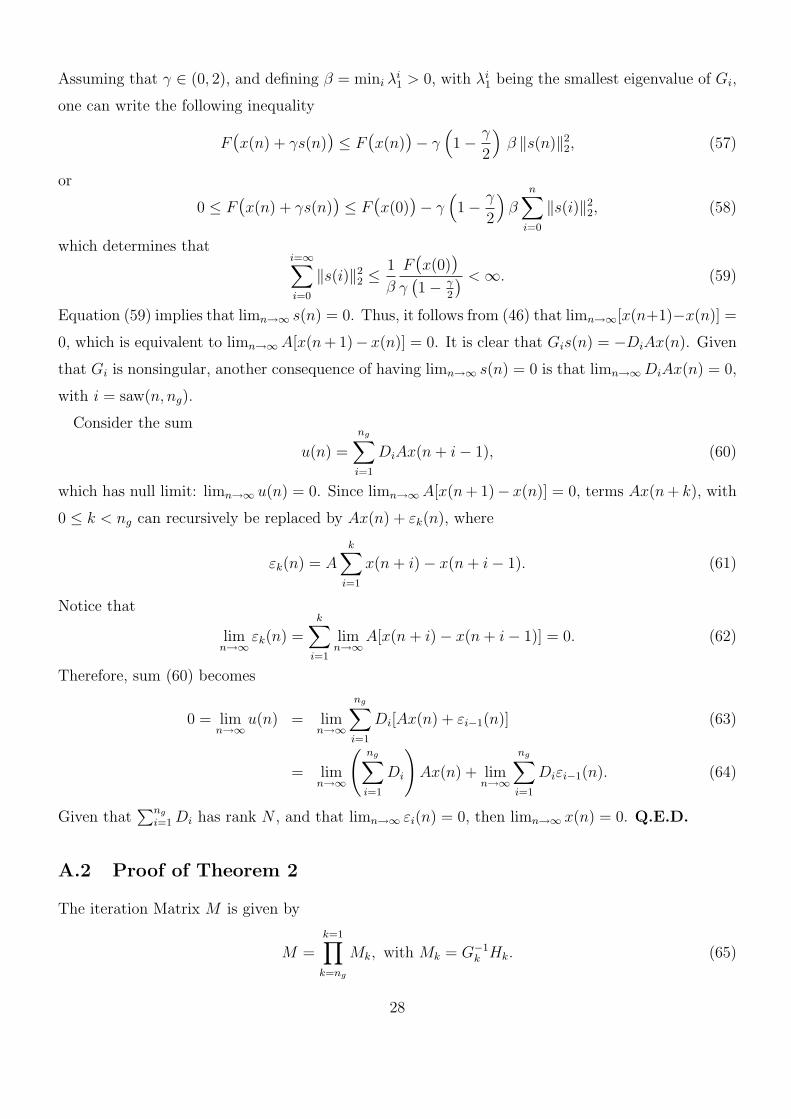
Assuming that γ ∈ (0, 2), and defining β = mini λi1 > 0, with λi
1 being the smallest eigenvalue of Gi,
one can write the following inequality
F(x(n) + γs(n)) ≤ F(x(n))− γ(1 − γ
2
)β ∥s(n)∥2
2, (57)
or
0 ≤ F(x(n) + γs(n)) ≤ F(x(0))− γ(1 − γ
2
)β
n∑i=0
∥s(i)∥22, (58)
which determines thati=∞∑i=0
∥s(i)∥22 ≤
1
β
F(x(0))γ(1 − γ
2
) < ∞. (59)
Equation (59) implies that limn→∞ s(n) = 0. Thus, it follows from (46) that limn→∞[x(n+1)−x(n)] =
0, which is equivalent to limn→∞ A[x(n + 1)− x(n)] = 0. It is clear that Gis(n) = −DiAx(n). Given
that Gi is nonsingular, another consequence of having limn→∞ s(n) = 0 is that limn→∞ DiAx(n) = 0,
with i = saw(n, ng).
Consider the sum
u(n) =
ng∑i=1
DiAx(n + i − 1), (60)
which has null limit: limn→∞ u(n) = 0. Since limn→∞ A[x(n + 1)− x(n)] = 0, terms Ax(n + k), with
0 ≤ k < ng can recursively be replaced by Ax(n) + εk(n), where
εk(n) = A
k∑i=1
x(n + i) − x(n + i − 1). (61)
Notice that
limn→∞
εk(n) =k∑
i=1
limn→∞
A[x(n + i) − x(n + i − 1)] = 0. (62)
Therefore, sum (60) becomes
0 = limn→∞
u(n) = limn→∞
ng∑i=1
Di[Ax(n) + εi−1(n)] (63)
= limn→∞
(ng∑i=1
Di
)Ax(n) + lim
n→∞
ng∑i=1
Diεi−1(n). (64)
Given that∑ng
i=1 Di has rank N , and that limn→∞ εi(n) = 0, then limn→∞ x(n) = 0. Q.E.D.
A.2 Proof of Theorem 2
The iteration Matrix M is given by
M =k=1∏k=ng
Mk, with Mk = G−1k Hk. (65)
28
Matrices G−1k with k = 1, · · · , ng exist, since their determinants are those of submatrices obtained
from A by choosing rows r and columns c, such that r, c ∈ Sk. But these submatrices have, by
hypothesis, non-null determinant.
Denote the i-th row of matrix Mk by [Mk]i. Having in account Definition 2 (matrices Gk and Hk),
and remembering that segmentation g1(D) is under assumption, it follows that the first k − 1 rows
verify
[Mk]i = [δ(j − i), j = 1, . . . , N ] = ei, j = 1, . . . , k − 1. (66)
Suppose that
[Mk]k = [∗, · · · , ∗︸ ︷︷ ︸k−1
, 0, · · · , 0], (67)
where the symbol ∗ denotes an arbitrary real number. An immediate consequence of (66) and (67)
is that
[MkMk−1 · · · ,M1]j = 0, 1 ≤ j ≤ k, k < ng. (68)
This can be checked by finite induction. On the other hand, segmentation g1(D) implies that
[Mng ]j = [∗, · · · , ∗︸ ︷︷ ︸N−D
, 0, · · · , 0], ng ≤ j ≤ N. (69)
Thus, it follows that M = 0.
To finish the proof, assumption (67) has to be proved. Since A−1 and G−1k , k = 1, . . . , ng exist,
then
DkA = (Gk − Hk), (70)
Dk = (Gk − Hk)A−1, (71)
G−1k Dk = (I − G−1
k Hk)A−1, (72)
[G−1k Dk]k = [A−1]k − [G−1
k Hk]kA−1. (73)
Consider matrix M1; rows [G−11 D1]1 and [A−1]1 have the following pattern:
[G−11 D1]1 = [∗, · · · , ∗︸ ︷︷ ︸
D
, 0, · · · , 0], (74)
[A−1]1 = [∗, · · · , ∗︸ ︷︷ ︸B
, 0, · · · , 0], (75)
where D ≥ B by hypothesis. Thus, one must have, from (73)
[G−11 Hk]1A
−1 = [∗, · · · , ∗︸ ︷︷ ︸D
, 0, · · · , 0]. (76)
29
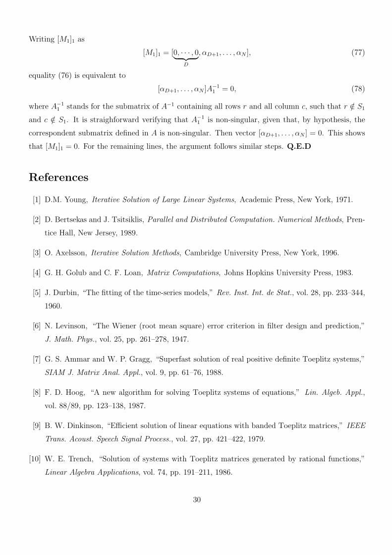
Writing [M1]1 as
[M1]1 = [0, · · · , 0︸ ︷︷ ︸D
, αD+1, . . . , αN ], (77)
equality (76) is equivalent to
[αD+1, . . . , αN ]A−11 = 0, (78)
where A−11 stands for the submatrix of A−1 containing all rows r and all column c, such that r /∈ S1
and c /∈ S1. It is straighforward verifying that A−11 is non-singular, given that, by hypothesis, the
correspondent submatrix defined in A is non-singular. Then vector [αD+1, . . . , αN ] = 0. This shows
that [M1]1 = 0. For the remaining lines, the argument follows similar steps. Q.E.D
References
[1] D.M. Young, Iterative Solution of Large Linear Systems, Academic Press, New York, 1971.
[2] D. Bertsekas and J. Tsitsiklis, Parallel and Distributed Computation. Numerical Methods, Pren-
tice Hall, New Jersey, 1989.
[3] O. Axelsson, Iterative Solution Methods, Cambridge University Press, New York, 1996.
[4] G. H. Golub and C. F. Loan, Matrix Computations, Johns Hopkins University Press, 1983.
[5] J. Durbin, “The fitting of the time-series models,” Rev. Inst. Int. de Stat., vol. 28, pp. 233–344,
1960.
[6] N. Levinson, “The Wiener (root mean square) error criterion in filter design and prediction,”
J. Math. Phys., vol. 25, pp. 261–278, 1947.
[7] G. S. Ammar and W. P. Gragg, “Superfast solution of real positive definite Toeplitz systems,”
SIAM J. Matrix Anal. Appl., vol. 9, pp. 61–76, 1988.
[8] F. D. Hoog, “A new algorithm for solving Toeplitz systems of equations,” Lin. Algeb. Appl.,
vol. 88/89, pp. 123–138, 1987.
[9] B. W. Dinkinson, “Efficient solution of linear equations with banded Toeplitz matrices,” IEEE
Trans. Acoust. Speech Signal Process., vol. 27, pp. 421–422, 1979.
[10] W. E. Trench, “Solution of systems with Toeplitz matrices generated by rational functions,”
Linear Algebra Applications, vol. 74, pp. 191–211, 1986.
30
[11] W. E. Trench, “Toeplitz systems associated with the product of a formal Laurent series and a
Laurent polynomial,” SIAM Journal on Matrix Analysis and Applications, vol. 9, pp. 181–193,
1988.
[12] M. R. Hestenes and E. L. Stiefel, “Methods of conjugate gradients for solving linear systems,”
J. Res. Nat. Bur. Standards Sect. 5, vol. 49, pp. 409–436, 1952.
[13] D. Luenberger, Linear and Nonlinear Programming, Addison Wesley Publishing Company,
Reading, Massachusetts, 1984, 2nd Edition.
[14] G. Strang, “A proposal for Toepliz matrix calculations,” Stud. Appl. Math., vol. 74, pp. 171–176,
1986.
[15] T. F. Chan, “An optimal circular preconditioner for Toeplitz systems,” SIAM J. Sci. Stat.
Comput., vol. 9, pp. 766–771, 1988.
[16] T. Ku and C. Kuo, “Design and analysis of optimal Toeplitz preconditioners,” IEEE Transac-
tions on Signal Processing, vol. 40, pp. 129–141, 1992.
[17] H. C. Andrews and B. R. Hunt, Digital Image Restoration, Prentice Hall, New Jersey, 1977.
[18] A. Tikhonov, A. Goncharsky, and V. Stepanov, “Inverse problems in image processing,” in
Ill-Posed Problems in the Natural Sciences, A. Tikhonov and A. Goncharsky, Eds., pp. 220–232.
Mir Publishers, Moscow, 1987.
[19] T. Chan and J. Shen, Image Processing and Analysis: Variational, PDE, Wavelet, and Stochas-
tic Methods, SIAM, 2005.
[20] R. S. Varga, Matrix Iterative Analysis, Prentice-Hall, Englehood Cliffs, NG, 1962.
[21] R. Beauwens, “Iterative solutions methods,” Appl. Numer. Math., vol. 51, pp. 437–450, 2004.
[22] A. M. Ostrowski, “Iterative solution of linear systems of functional equations,” J. Math. Anal.
App., vol. 2, pp. 351–369, 1961.
[23] L. Lapidus and G. F. Pinder, Numerical Solution of Partial Differential Equations in Science
and Engineering, John Wiley & Sons, New York, 1982.
[24] D. O’Leary and R. E. White, “Multi-splittings of matrices and parallel solutions of linear
systems,” SIAM J. Algebric Discrete Math., vol. 6,, pp. 630–640, 1985.
31
[25] O. A. Mcbryan and E. Van de Velde, “Parallel algorithms for elliptic equations,” Comm. Pure
Appl. Math., vol. 38, pp. 769–795, 1985.
[26] M. Newmann and R. J. Plemmons, “Convergence of parallel multisplittings and iterative meth-
ods for M-matrices,” Linear algebra Appl., vol. 88/89, pp. 559–573, 1987.
[27] R. E. White, “Multisplittings of a symmetric positive definite matrix,” SIAM J. Matrix Anal.
Appl., vol. 11, pp. 69–82, 1990.
[28] L. J. Hayes, “A vectorized matrix-vector multiply and overlapping block iterative method,” in
Supercomputer Applications, R.W. Numrich, Ed., pp. 91–100. Plenum Press, New York, 1984.
[29] W. Hackbush, Multi-Grid Methods and Applications, Springer-Verlag, New York, 1985.
[30] D. J. Evans, Preconditioning Methods: Analysis and Applications, Gordon and Breach, New
York, 1983.
[31] T. Ku and C. Kuo, “Spectral properties of preconditioned rational Toeplitz matrices,” SIAM
Journal on Matrix Analysis and Application, vol. 14, pp. 146–165, 1993.
[32] A. Jain, Fundamentals of Digital Image Processing, Prentice Hall, Englewood Cliffs, 1989.
[33] A. Blake and A. Zisserman, Visual Reconstruction, MIT Press, Cambridge, M.A., 1987.
[34] D. Geiger and F. Girosi, “Parallel and deterministic algorithms from MRF’s: Surface recon-
struction,” IEEE Transactions on Pattern Analysis and Machine Intelligence, vol. PAMI-13,
no. 5, pp. 401–412, May 1991.
[35] M. Figueiredo and J. Leitao, “Simulated tearing: an algorithm for discontinuity preserving
visual suraface reconstruction,” in Proceedings of the IEEE Computer Society Conference on
Computer Vision and Pattern Recognition – CVPR’93, New York, June 1993, pp. 28–33.