An overview of CFD tools and comparison of a 2D · PDF fileAn Overview of CFD Tools and...

An Overview of CFD Tools and Comparison of a 2D Testcase

CES Seminar Project Thesis

presented by

Moritz Begall

296113

Advisor: Alexandra Krieger, Ph.D.

Aachen, 01.09.2015

Abstract

This report presents an overview of two popular CFD tools, OpenFOAM and COMSOL Mul-

tiphysics.

It highlights their main features and differences, gives a short review of the finite-volume

and finite-element discretization methods, which are utilized by OpenFOAM and COMSOL,

respectively, and compares their performance in a simple test case.

Contents

List of Figures iv

List of Tables v

1. CFD Tools 1

1.1. OpenFOAM . . . . . . . . . . . . . . . . . . . . . . . . . . . . . . . . . . . 1

1.1.1. Usage . . . . . . . . . . . . . . . . . . . . . . . . . . . . . . . . . . 1

1.2. COMSOL . . . . . . . . . . . . . . . . . . . . . . . . . . . . . . . . . . . . . 4

1.2.1. Usage . . . . . . . . . . . . . . . . . . . . . . . . . . . . . . . . . . 4

1.3. Comparison of OpenFOAM and COMSOL . . . . . . . . . . . . . . . . . . . 5

2. The Finite Volume and Finite Element Method 7

2.1. Flow Equations . . . . . . . . . . . . . . . . . . . . . . . . . . . . . . . . . . 7

2.2. The Finite-Volume Method . . . . . . . . . . . . . . . . . . . . . . . . . . . 8

2.3. The Finite-Element Method . . . . . . . . . . . . . . . . . . . . . . . . . . . 12

3. Comparison of a 2D Testcase 15

3.1. Case Setup . . . . . . . . . . . . . . . . . . . . . . . . . . . . . . . . . . . . 15

3.1.1. OpenFOAM . . . . . . . . . . . . . . . . . . . . . . . . . . . . . . . 16

3.1.2. COMSOL . . . . . . . . . . . . . . . . . . . . . . . . . . . . . . . . 16

3.2. Results . . . . . . . . . . . . . . . . . . . . . . . . . . . . . . . . . . . . . . 16

3.2.1. Runtime Comparison . . . . . . . . . . . . . . . . . . . . . . . . . . . 18

4. Conclusion 20

Bibliography 21

A. OpenFOAM case files 23

A.1. Circular Obstacle . . . . . . . . . . . . . . . . . . . . . . . . . . . . . . . . . 23

A.2. Square Obstacle . . . . . . . . . . . . . . . . . . . . . . . . . . . . . . . . . 30

iii

List of Figures

1.1. The OpenFOAM case structure . . . . . . . . . . . . . . . . . . . . . . . . . 2

1.2. An exemplary OpenFOAM dictionary file . . . . . . . . . . . . . . . . . . . . 3

1.3. The COMSOL GUI . . . . . . . . . . . . . . . . . . . . . . . . . . . . . . . . 5

2.1. Discrete cells on a Cartesian grid . . . . . . . . . . . . . . . . . . . . . . . . 10

2.2. Piecewise linear shape functions . . . . . . . . . . . . . . . . . . . . . . . . . 14

3.1. The testcase grids . . . . . . . . . . . . . . . . . . . . . . . . . . . . . . . . 16

3.2. Testcase 1 . . . . . . . . . . . . . . . . . . . . . . . . . . . . . . . . . . . . 17

3.3. Testcase 2 . . . . . . . . . . . . . . . . . . . . . . . . . . . . . . . . . . . . 17

iv

List of Tables

3.1. Number of degrees of freedom . . . . . . . . . . . . . . . . . . . . . . . . . . 18

3.2. Runtime comparison . . . . . . . . . . . . . . . . . . . . . . . . . . . . . . . 18

4.1. CFD-tool quick comparison . . . . . . . . . . . . . . . . . . . . . . . . . . . 20

1. CFD Tools

This chapter will give an overview over the main features of OpenFOAM and COMSOL, as

well as their differences.

1.1. OpenFOAM

OpenFOAM (Open Field Operation and Manipulation) [1, 2, 3] is a free and open source

computational fluid dynamics (CFD) toolbox. It is developed by OpenCFD Ltd. and distributed

by the OpenFOAM Foundation under the GNU General Public License (GPL). The software

package is written in C++ and includes more than 80 solver applications covering a wide

range of continuum mechanics, such as structural mechanics, heat transfer, chemical reactions,

turbulence and multiphase flow. To solve the systems of partial differential equations describing

these phenomena, both the Finite Element Method and the Finite Volume Method have been

implemented, but the FVM is the method that is utilized by most solvers. The package also

contains tools for meshing, as well as pre- and post-processing.

Since the source code is freely available and anyone is allowed to use and modify it in any way,

the software is well-suited to be adapted for specific purposes or for the implementation of

new custom functions and solvers. However, documentation is very scarce and often insuffi-

cient, making modifications or the application of the software difficult, especially for new users.

1.1.1. Usage

OpenFOAM does not provide a graphical user interface (GUI), instead it is operated using the

command line interface (CLI) of a terminal emulator.

1

1. CFD Tools

To run simulations with OpenFoam, a mesh has to be generated. Unstructured meshes of

any shape are supported, cells can have any number of faces and corresponding neighbour

cells and the faces can have any number of edges. Faces are defined by means of their nodes

and all external faces need an identifier to be able to specify boundary conditions later on.

OpenFOAM is provided with two meshing utilities: blockMesh can be used for simple geome-

tries that consist of one or more blocks, e.g. a cylinder inside a channel, which have to be

specified in a text configuration file, called blockMeshDict. More complex geometries can

be discretized with snappyHexMesh, which generates a mesh from CAD objects like e.g. STL

files. It is also possible to convert meshes created with third-party software, e.g. ANSYS

GAMBIT.

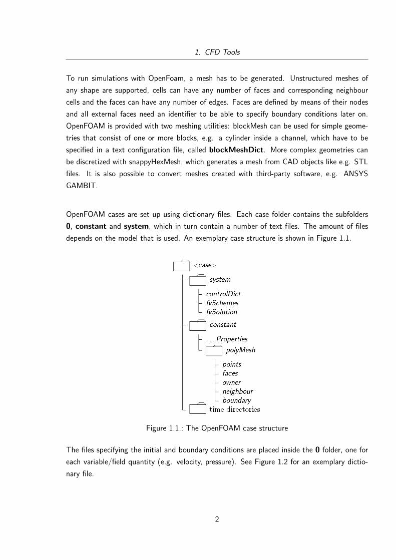
OpenFOAM cases are set up using dictionary files. Each case folder contains the subfolders

0, constant and system, which in turn contain a number of text files. The amount of files

depends on the model that is used. An exemplary case structure is shown in Figure 1.1.

Figure 1.1.: The OpenFOAM case structure

The files specifying the initial and boundary conditions are placed inside the 0 folder, one for

each variable/field quantity (e.g. velocity, pressure). See Figure 1.2 for an exemplary dictio-

nary file.

2

1. CFD Tools

/∗−−−−−−−−−−−−−−−−−−−−−−−−−−−−−−−−∗− C++−∗−−−−−−−−−−−−−−−−−−−−−−−−−−−−−−−−−−∗\| ========= | || \\ / F i e l d | OpenFOAM: The Open Source CFD Toolbox || \\ / O p e r a t i o n | Ve r s i on : 2 . 4 . 0 || \\ / A nd | Web : www.OpenFOAM. org || \\/ M a n i p u l a t i o n | |\∗−−−−−−−−−−−−−−−−−−−−−−−−−−−−−−−−−−−−−−−−−−−−−−−−−−−−−−−−−−−−−−−−−−−−−−−−−−−∗/FoamFile

version 2 . 0 ;format ascii ;class volVectorField ;object U ;

// ∗ ∗ ∗ ∗ ∗ ∗ ∗ ∗ ∗ ∗ ∗ ∗ ∗ ∗ ∗ ∗ ∗ ∗ ∗ ∗ ∗ ∗ ∗ ∗ ∗ ∗ ∗ ∗ ∗ ∗ ∗ ∗ ∗ ∗ ∗ ∗ ∗ //

dimensions [ 0 1 −1 0 0 0 0 ] ;

internalField uniform (0 0 0) ;

boundaryField

inlet

type fixedValue ;value uniform ( 1 . 2 0 0) ;

outlet

type zeroGradient ;

fixedWalls

type fixedValue ;value uniform (0 0 0) ;

frontAndBack

type empty ;

// ∗∗∗∗∗∗∗∗∗∗∗∗∗∗∗∗∗∗∗∗∗∗∗∗∗∗∗∗∗∗∗∗∗∗∗∗∗∗∗∗∗∗∗∗∗∗∗∗∗∗∗∗∗∗∗∗∗∗∗∗∗∗∗∗∗∗∗∗∗∗∗∗∗ //

Figure 1.2.: An exemplary OpenFOAM dictionary file (containing the specifcation of the initialand boundary conditions for the velocity field)

The constant folder contains the mesh and information on physical properties and constants,

e.g. densities or gravity.

The controlDict inside the system folder specifies solver settings such as the start- and end-

time of the simulation, the timestep and output options. The fvSchemes dictionary in the

same directory sets the numerical schemes for terms, such as derivatives in equations, that

appear in the applications. Finally, fvSolution specifies the numerical methods to solve for

the individual variables.

For every solver, at least one tutorial case is included in the software package to familiarize the

user with the actual dictionaries required by the solver and the parameters therein. Nonetheless

it is often not documented which values a certain parameter can take, how this affects the

3

1. CFD Tools

simulation, or if it is needed at all. Therefore, it is sometimes necessary to rely on the findings

of other users or on trial and error.

After running a case, the obtained results can be displayed and post-processed with ParaView

or other applications.

1.2. COMSOL

COMSOL was founded in Stockholm, Sweden in 1986 by two graduate students of the Royal

Institute of Technology. The company now has offices all over the world and employs 420

people. Its main product is the finite element analysis (FEA) program COMSOL Multiphysics.

COMSOL Multiphysics covers an even greater range of physics than OpenFOAM, from struc-

tural mechanics to electromechanics, fluid flow, heat transfer, chemical reactions, acoustics,

microfluidics and more.

One of the main features is the easy implementation of multiphysics couplings. For example,

one might examine the thermal expansion of a structure subject to a heat load, which might

in turn be caused by an electric current.

Because COMSOL Multiphysics is a complete FEA program, it can be used for the whole

analysis process of a case. This means that not only the actual simulations, but everything

from pre- to post-processing can be performed with COMSOL. However, it is still possible to

im- or export data (e.g. CAD files) from or to other applications.

1.2.1. Usage

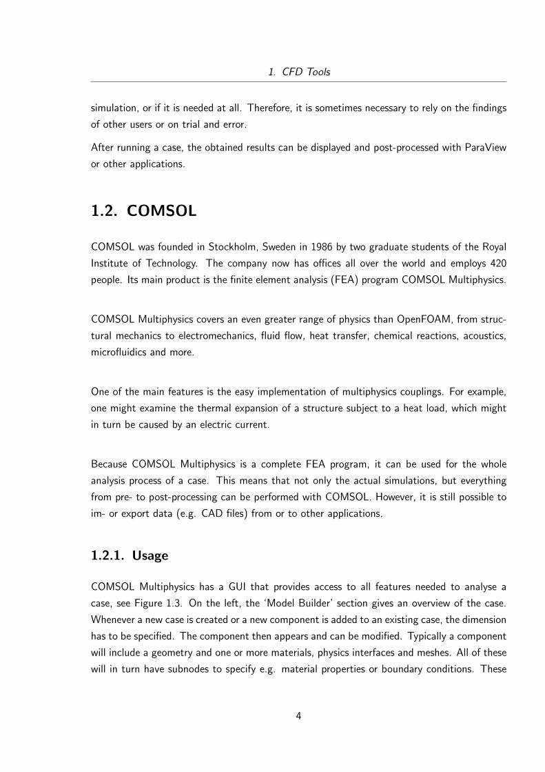
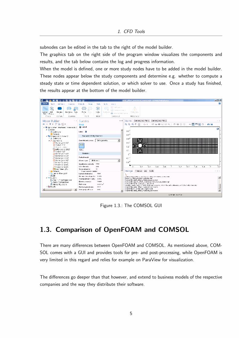
COMSOL Multiphysics has a GUI that provides access to all features needed to analyse a

case, see Figure 1.3. On the left, the ‘Model Builder’ section gives an overview of the case.

Whenever a new case is created or a new component is added to an existing case, the dimension

has to be specified. The component then appears and can be modified. Typically a component

will include a geometry and one or more materials, physics interfaces and meshes. All of these

will in turn have subnodes to specify e.g. material properties or boundary conditions. These

4

1. CFD Tools

subnodes can be edited in the tab to the right of the model builder.

The graphics tab on the right side of the program window visualizes the components and

results, and the tab below contains the log and progress information.

When the model is defined, one or more study nodes have to be added in the model builder.

These nodes appear below the study components and determine e.g. whether to compute a

steady state or time dependent solution, or which solver to use. Once a study has finished,

the results appear at the bottom of the model builder.

Figure 1.3.: The COMSOL GUI

1.3. Comparison of OpenFOAM and COMSOL

There are many differences between OpenFOAM and COMSOL. As mentioned above, COM-

SOL comes with a GUI and provides tools for pre- and post-processing, while OpenFOAM is

very limited in this regard and relies for example on ParaView for visualization.

The differences go deeper than that however, and extend to business models of the respective

companies and the way they distribute their software.

5

1. CFD Tools

OpenFOAM is open source software and is free to use, modify and redistribute. However,

using it can be quite difficult and the provided user guide serves only as an overview, not an

exhaustive knowledge base. OpenCFD earns money by offering different support packages,

ranging from simple assistance in case setup to customized solvers for specific applications [4].

COMSOL Multiphysics on the other hand requires the purchase of a license. Additionally,

as is typical with proprietary software, no source code is provided. COMSOL does provide

thorough documentation, as well as an online forum to talk to support staff and other users, a

blog discussing features of the program and how to use them to solve specific problems, and

a variety of workshops and tutorials.

6

2. The Finite Volume and Finite Element

Method

This chapter discusses some of the fundamental theoretical aspects of computational fluid

dynamics.

Section 2.1 shortly introduces the governing equations. Section 2.2 presents the basics of the

Finite-Volume Method, which is utilized by OpenFOAM, and Section 2.3 does the same for

the Finite-Element Method used by COMSOL.

2.1. Flow Equations

In computational fluid dynamics, newtonian fluids are described by the Navier-Stokes equations

[5]. These equations for continuity, momentum and energy, respectively, are the following:

∂ρ

∂t+∇ · (ρ~v) = 0

∂ρ~v

∂t+∇ ·

(ρ~v~v −~~σ

)= ~fvol

∂ρE

∂t+∇ ·

(ρE~v −~~σ · ~v + ~q

)= ~fvol · ~v

In these equations, ρ is the density,~~σ is the stress tensor resulting from friction within the

fluids, ~q denotes the heat flux, E the inner energy of the fluids and ~fvol volume forces such as

gravity. The velocity vector ~v is often denoted in the literature by U, and this notation will

be used from now on.

The equations simplify considerably under the assumption of constant density: The continuity

equation reduces to

∇ ·U = 0, (2.1)

7

2. The Finite Volume and Finite Element Method

hence the velocity field is a solenoidal (divergence-free) vector field. As a consequence, the

pressure is no longer coupled to density and temperature. As a result, and with the additional

assumption of constant viscosity, the energy equation and the continuity and momentum equa-

tions can be decoupled. Because the temperature of the fluid is not of concern here, the energy

equation can be neglected.

The assumption that the density is constant is reasonable because the fluid modeled by the

Navier Stokes equations is a slow-moving liquid.

The momentum equation can be rewritten (see e.g. [6]) as follows

ρ∂U

∂t+∇ · (ρUU) = −∇p+ µ∇2U + ρ−→g +

−→F s, (2.2)

where−→F s represents the surface tension force

−→F s = σκn

with the surface tension coefficient σ, the unit vector normal to the interface n and the

interface curvature κ, the latter two are defined as

n =∇α|∇α|

κ = ∇ · n.

In summary, isothermal and incompressible flow is governed by (2.1) and (2.2). They have

to be discretized to numerically calculate their solution. Two different ways to discretize the

equations are presented in Sections 2.2 and 2.3.

2.2. The Finite-Volume Method

The finite-volume method (FVM) [7, 8] is a method for the numerical solution of partial

differential equations. In the field of computational fluid dynamics, these equations describe

8


conservation laws, i.e. the conservation of mass, momentum and energy. In general, a con-

servation law states that a certain property in a closed, isolated system remains constant over

time. An example is the generic equation

∂φ

∂t+∇ · ~F (φ) = s (2.3)

with a scalar quantity φ, a flow vector ~F (φ) and a source term s. If the source term is equal

to zero and no flow occurs, φ does not change.

The FVM requires two steps. The equation of interest is integrated over a control volume Ω

that is constant over time, and is then transformed by the divergence theorem into a volume-

and a surface integral, which can then be discretized independently. Applying these steps to

(2.3) yields

∂

∂t

∫Ω

φ dV +

∫Ω

∇ · ~F (φ)dV =

∫Ω

s dV, (2.4)

which is equivalent to

∂

∂t

∫Ω

φ dV +

∮∂Ω

~F (φ) · d ~A =

∫Ω

s dV. (2.5)

Now the balance over a finite volume Vj can be taken, resulting in

∂

∂t(φj∆Vj) +

∑cellfaces

~F (φi) · d ~A = sj∆Vj. (2.6)

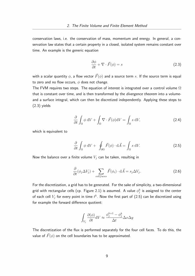
For the discretization, a grid has to be generated. For the sake of simplicity, a two-dimensional

grid with rectangular cells (cp. Figure 2.1) is assumed. A value φkj is assigned to the center

of each cell Vj for every point in time tk. Now the first part of (2.5) can be discretized using

for example the forward difference quotient:

∫Vj

∂(φ)

∂tdV ≈

φk+1j − φkj

∆t∆x∆y

The discretization of the flux is performed separately for the four cell faces. To do this, the

value of ~F (φ) on the cell boundaries has to be approximated.

9


Figure 2.1.: Discrete cells on a cartesian grid [9]

The discretization method used should be suitable for the problem or equation. If the flux is

governed by diffusion, central differences are the method of choice, because diffusion describes

a balancing process that does not have a specific direction.

If, on the other hand, the flux is dominated by convection, the flow direction plays an impor-

tant role. In this case, an upwind discretization scheme should be applied [7, 10].

Often, convection and diffusion occur simultaneously and have to be accounted for. In the

case of the convection-diffusion equation, the flow vector has the form

~F (φ) = Uφ−D∇φ

with the diffusion coefficient D. The discretization of the flux will be demonstrated exemplarily

for horizontal flow over the right (eastern) cell face. ~F (φ) reduces to

f(φ) = uφ−D∂φ∂x

(2.7)

where u is the component of U in the direction of the x-axis. The value on the cell boundary is

designated with the subscript e, the values at the cell centers to the left and right are denoted

with the subscripts P and E, respectively. Discretizing the diffusive part of (2.7) with central

differences yields

10


fe = ueφe −DφE − φP∆xEP

.

The value of φe is still undefined. Because it is part of the convective part of the equation,

instead of taking an average of the form

φe =φE + φP

2,

φe is set to the value upstream of the boundary. This full upwind discretization renders the

following one sided formulation:

ueφe =

ueφP ue > 0

ueφE ue < 0

Once fe, and analogous fw, fn and fs (the flow over the left, top and bottom cell boundaries)

have been fully discretized, the surface integral in (2.5) can be approximated:

∮∂Vi

~F (φi) · d ~A ≈ (fe − fw)∆y + (gn − gs)∆x

In practice, there are many other and more advanced discretization schemes. The ability to

choose different schemes that are suited to different equations is one advantage of the FVM.

Another strength is its ability to work on unstructured meshes [8].

The main steps of the FVM will now be applied to the continuity and momentum equations,

because they are the equations of interest. For the continuity equation, this yields:

∂ρ

∂t+∇ · (ρU) = 0

⇒ ∂

∂t

∫Ω

ρ dV +

∫Ω

∇ · (ρU)dV = 0

⇔ ∂

∂t

∫Ω

ρ dV +

∮∂Ω

ρU · d ~A = 0

Here, ρU is called the mass flux. It can be seen that the change of mass within the volume V

over time is equal to the flow over the surface or boundary. Again, the balance over a finite

volume Vj is applied, giving

11


∂

∂t(ρj∆Vj) +

∑cellfaces

ρiUi · d ~A = 0.

Applying the same steps to the momentum equation results in

∂

∂t(ρjUj∆Vj) +

∑cellfaces

ρiUi · d ~A = 0.

2.3. The Finite-Element Method

The finite-element method rests upon the discrete representation of a weak integral form of

the partial differential equation to be solved [10]. To derive the weak form, two classes of

functions are needed, namely the test functions and trial solutions.

The test functions are all functions which are square integrable, have square integrable first

derivatives over the computational domain Ω, and vanish on the Dirichlet part ΓD of the

boundary. They are defined by

V = w ∈ H1(Ω) | w = 0 on ΓD,

where H1(Ω) is a Sobolev space. The trial solutions are similar, except in that they are

required to satisfy the Dirichlet conditions on ΓD:

S = u ∈ H1(Ω) | u = uD on ΓD.

For simplicity, the main steps of the finite-element method will be demonstrated using the

Poisson equation

−∇2u = s in Ω, (2.8)

with u = uD on ΓD and n · ∇u = h on ΓN (the Neumann part of the boundary).

The first step is to multiply the equation of interest with a test function w and to integrate

over Ω:

−∫

Ω

w ∇2u dΩ =

∫Ω

w s dΩ (2.9)

12


Then the Green-Gauss divergence theorem is applied to the left hand side of (2.9):

−∫

Ω

w ∇2u dΩ = −∫

Ω

(∇ · (w∇u)−∇w · ∇u) dΩ

=

∫Ω

∇w · ∇u dΩ−∫

Γ

w(n · ∇u)dΓ

This changes the requirements on u, it now only has to be once differentiable, as has w.

Inserting the Neumann boundary condition gives the weak form of (2.8):∫Ω

∇w · ∇u dΩ =

∫Ω

w s dΩ +

∫ΓN

w h dΓ (2.10)

Obviously, any solution to the original problem (2.8) is a solution to the weak problem. It can

be shown by means of the Lax-Milgram lemma [10] that a solution to the weak problem is

unique and is therefore identical to the strong solution, if the latter exists.

Now (2.10) can be discretized by partitioning the computational domain Ω into a finite number

of subdomains, or elements.

Ω =⋃

Ωe

and Ωe ∩ Ωf = ∅ for e 6= f

Similarly, finite dimensional subspaces of the test function and trial solution spaces are de-

fined,V h := w ∈ H1(Ω) | w|Ωe ∈ Pm(Ωe) ∀e and w = 0 on ΓD

Sh := u ∈ H1(Ω) | u|Ωe ∈ Pm(Ωe) ∀e and u = uD on ΓD,

where Pm is the finite element interpolating space.

The finite-element formulation is then obtained by restricting (2.10) to V h and Sh:∫Ω

∇wh · ∇uh dΩ =

∫Ω

wh s dΩ +

∫ΓN

wh h dΓ (2.11)

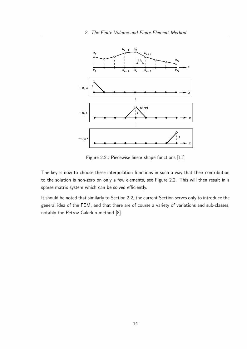
In the (Bubnow-) Galerkin method, the test functions are taken equal to the interpolation or

shape functions Nj.

uh =N∑i=1

uiNi, wh = Nj

13


Figure 2.2.: Piecewise linear shape functions [11]

The key is now to choose these interpolation functions in such a way that their contribution

to the solution is non-zero on only a few elements, see Figure 2.2. This will then result in a

sparse matrix system which can be solved efficiently.

It should be noted that similarly to Section 2.2, the current Section serves only to introduce the

general idea of the FEM, and that there are of course a variety of variations and sub-classes,

notably the Petrov-Galerkin method [8].

14

3. Comparison of a 2D Testcase

To compare the OpenFOAM and COMSOL solvers, the Karman vortex street was chosen as

a simple, 2D laminar test case. The Karman vortex street is a well known phenomenon and

frequently used as an example or test case. Indeed, the test case presented here was besed on

a COMSOL tutorial case [12].

3.1. Case Setup

The test case that was chosen consists of a two-dimensional channel with an obstacle. Fluid

flows in from the left and out to the right. The channel has a length of 2.4m and a height

of 0.4m. The inflow velocity was set to 1.2ms

. The kinematic viscosity ν was set to 0.001m2

s,

resulting in a Reynolds number of Re= Ulν

=480 (with the characteristic length l set to the

channel height). The flow is thus in the laminar regime, as the critical Reynolds number for

channel flows is in the range 2300-4000.

Placing the obstacle in the middle of the channel results in a symmetric, stationary flow profile.

When introducing an irregularity by moving the obstacle a little closer to the upper channel

wall, however, a Karman vortex street forms.

The test case was run with two variations, once with a circular obstacle and 8104 grid cells or

elements, and once with a square obstacle and 32816 cells. In each instance, the grid was first

generated in COMSOL and then, lacking the option to convert to a format OpenFOAM can

read, defined for OpenFOAM by writing the respective mesh dictionaries by hand using the

same parameters. This ensured that identical meshes were used by COMSOL and OpenFOAM.

They are shown in Figure 3.1. In both cases, 6 real-time seconds of fluid flow were simulated.

15


Figure 3.1.: The testcase grids

3.1.1. OpenFOAM

For the OpenFOAM simulations, the icoFoam solver was selected. OpenFOAM version 2.4

was used. All dictionary files needed to rerun the cases are included in appendix A.

3.1.2. COMSOL

COMSOL Multiphysics version 5.0 was used. A laminar single phase flow physics interface

was utilized, selecting incompressible flow and leaving all other settings at their defaults. The

velocity field was initialized to 0ms

, and the inlet velocity had to be ramped up from 0ms

, as

the solver would not converge when starting with 1.2ms

right away.

3.2. Results

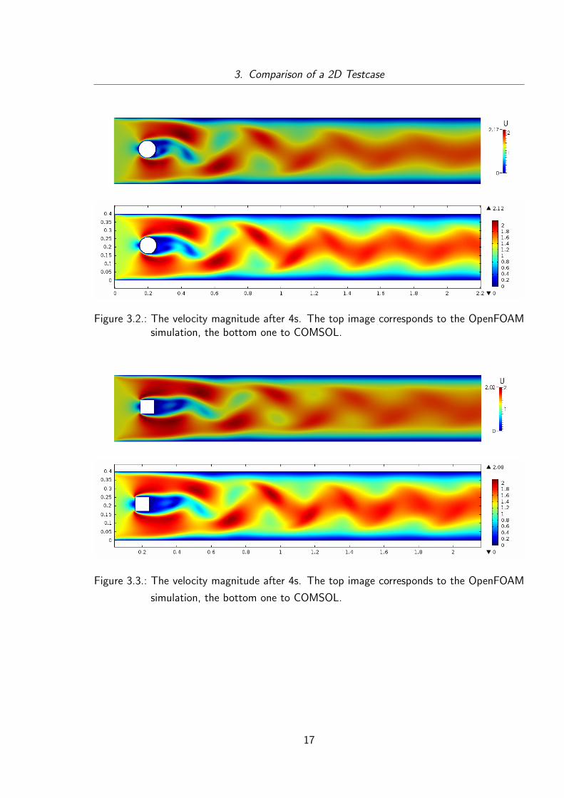
Figures 3.2 and 3.3 show the velocity magnitude of the fluid. It can be seen that the flow

fields generally look similar, as they should. Changing the shape of the obstacle or the number

of cells does not change the result qualitatively, as the vortex street forms in both cases.

However, the velocity field obtained by the simulation with OpenFOAM appears to be a bit

washed out, indicating a higher influence of diffusion.

16


Figure 3.2.: The velocity magnitude after 4s. The top image corresponds to the OpenFOAMsimulation, the bottom one to COMSOL.

Figure 3.3.: The velocity magnitude after 4s. The top image corresponds to the OpenFOAM

simulation, the bottom one to COMSOL.

17


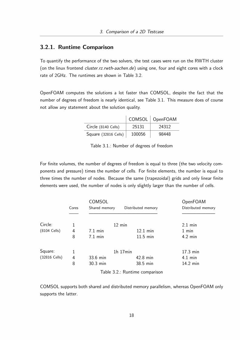
3.2.1. Runtime Comparison

To quantify the performance of the two solvers, the test cases were run on the RWTH cluster

(on the linux frontend cluster.rz.rwth-aachen.de) using one, four and eight cores with a clock

rate of 2GHz. The runtimes are shown in Table 3.2.

OpenFOAM computes the solutions a lot faster than COMSOL, despite the fact that the

number of degrees of freedom is nearly identical, see Table 3.1. This measure does of course

not allow any statement about the solution quality.

COMSOL OpenFOAM

Circle (8140 Cells) 25131 24312

Square (32816 Cells) 100056 98448

Table 3.1.: Number of degrees of freedom

For finite volumes, the number of degrees of freedom is equal to three (the two velocity com-

ponents and pressure) times the number of cells. For finite elements, the number is equal to

three times the number of nodes. Because the same (trapezoidal) grids and only linear finite

elements were used, the number of nodes is only slightly larger than the number of cells.

Circle:(8104 Cells)

Square:(32816 Cells)

Cores

——

148

148

COMSOLShared memory Distributed memory

——————————————–

12 min7.1 min 12.1 min7.1 min 11.5 min

1h 17min33.6 min 42.8 min30.3 min 38.5 min

OpenFOAMDistributed memory

———————

2.1 min1 min4.2 min

17.3 min4.1 min14.2 min

Table 3.2.: Runtime comparison

COMSOL supports both shared and distributed memory parallelism, whereas OpenFOAM only

supports the latter.

18


It can be seen that the computation runs faster when using shared memory, as expected. Fur-

thermore, the test cases seem to be too small to gain a meaningful speedup from computation

on more than four cores. In fact, OpenFOAM takes longer to compute the solution when using

eight cores, indicating that most time is utilized for the intercommunication of the cores.

One other interesting thing to note is that OpenFOAM shows superlinear speedup when switch-

ing from one to four cores. This could be due to to the fact that dividing the problem leads

to fewer cache misses, avoiding reloading data from RAM.

19

4. Conclusion

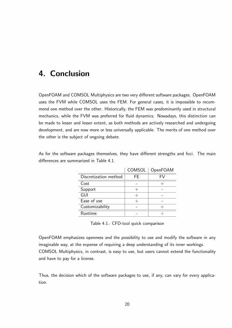
OpenFOAM and COMSOL Multiphysics are two very different software packages. OpenFOAM

uses the FVM while COMSOL uses the FEM. For general cases, it is impossible to recom-

mend one method over the other. Historically, the FEM was predominantly used in structural

mechanics, while the FVM was preferred for fluid dynamics. Nowadays, this distinction can

be made to lesser and lesser extent, as both methods are actively researched and undergoing

development, and are now more or less universally applicable. The merits of one method over

the other is the subject of ongoing debate.

As for the software packages themselves, they have different strengths and foci. The main

differences are summarized in Table 4.1.

COMSOL OpenFOAM

Discretization method FE FV

Cost - +Support + -GUI + -Ease of use + -Customizability - +

Runtime - +

Table 4.1.: CFD-tool quick comparison

OpenFOAM emphasizes openness and the possibility to use and modify the software in any

imaginable way, at the expense of requiring a deep understanding of its inner workings.

COMSOL Multiphysics, in contrast, is easy to use, but users cannot extend the functionality

and have to pay for a license.

Thus, the decision which of the software packages to use, if any, can vary for every applica-

tion.

20

Bibliography

[1] Features of OpenFOAM. http://www.openfoam.org/features/.

[2] C. Greenshields. User Guide. OpenFOAM Foundation Ltd., http://foam.

sourceforge.net/docs/Guides-a4/UserGuide.pdf, 2.4.0 edition, 2015.

[3] C. Greenshields. Programmer’s Guide. OpenFOAM Foundation Ltd., http://foam.

sourceforge.net/docs/Guides-a4/ProgrammersGuide.pdf, 2.4.0 edition, 2015.

[4] OpenFOAM software support. http://www.openfoam.com/support/.

[5] W. Schroder. Fluidmechanik, volume 7 of Aachener Beitrage zur Stromungsmechanik.

Mainz, 3 edition, 2010.

[6] S. M. Damian. Description and utilization of interfoam multiphase solver. Techni-

cal report, Universidad Nacional del Litoral, http://infofich.unl.edu.ar/upload/

3be0e16065026527477b4b948c4caa7523c8ea52.pdf.

[7] B. Binninger. Numerische Simulation von Stromungsvorgangen. Vorlesungsskript, RWTH

Aachen, 2012.

[8] Hirsch C. Numerical Computation of Internal and External Flows, volume 1 of Funda-

mentals of Computational Fluid Dynamics. Butterworth-Heinemann, 2 edition, 2007.

[9] Finite volume methods. http://ocw.mit.edu/courses/mechanical-engineering/

2-29-numerical-fluid-mechanics-fall-2011/lecture-notes/MIT2_29F11_

lect_18.pdf, 2011. Lecture Notes, Massachusetts Institute of Technology.

[10] J. Donea and A. Huerta. Finite Element Methods for Flow Problems. Wiley, 2003.

[11] Joaquim Peiro and Spencer Sherwin. Finite difference, finite element and finite volume

methods for partial differential equations. In Sidney Yip, editor, Handbook of Materials

Modeling, pages 2415–2446. Springer Netherlands, 2005.

21

http://www.openfoam.org/features/

http://foam.sourceforge.net/docs/Guides-a4/UserGuide.pdf

http://foam.sourceforge.net/docs/Guides-a4/UserGuide.pdf

http://foam.sourceforge.net/docs/Guides-a4/ProgrammersGuide.pdf

http://foam.sourceforge.net/docs/Guides-a4/ProgrammersGuide.pdf

http://www.openfoam.com/support/

http://infofich.unl.edu.ar/upload/3be0e16065026527477b4b948c4caa7523c8ea52.pdf

http://infofich.unl.edu.ar/upload/3be0e16065026527477b4b948c4caa7523c8ea52.pdf

http://ocw.mit.edu/courses/mechanical-engineering/2-29-numerical-fluid-mechanics-fall-2011/lecture-notes/MIT2_29F11_lect_18.pdf



Bibliography

[12] Flow past a cylinder. http://www.comsol.com/model/download/215601/models.

mph.cylinder_flow.pdf.

22

http://www.comsol.com/model/download/215601/models.mph.cylinder_flow.pdf

http://www.comsol.com/model/download/215601/models.mph.cylinder_flow.pdf

A. OpenFOAM case files

A.1. Circular Obstacle


version 2 . 0 ;

format ascii ;

class volScalarField ;

object p ;

// ∗ ∗ ∗ ∗ ∗ ∗ ∗ ∗ ∗ ∗ ∗ ∗ ∗ ∗ ∗ ∗ ∗ ∗ ∗ ∗ ∗ ∗ ∗ ∗ ∗ ∗ ∗ ∗ ∗ ∗ ∗ ∗ ∗ ∗ ∗ ∗ ∗ //

dimensions [ 0 2 −2 0 0 0 0 ] ;

internalField uniform 0 ;

boundaryField

inlet

type zeroGradient ;

outlet

type fixedValue ;

value uniform 0 ;

fixedWalls

type zeroGradient ;

frontAndBack

type empty ;

// ∗∗∗∗∗∗∗∗∗∗∗∗∗∗∗∗∗∗∗∗∗∗∗∗∗∗∗∗∗∗∗∗∗∗∗∗∗∗∗∗∗∗∗∗∗∗∗∗∗∗∗∗∗∗∗∗∗∗∗∗∗∗∗∗∗∗∗∗∗∗∗∗∗ //

/∗−−−−−−−−−−−−−−−−−−−−−−−−−−−−−−−−∗− C++−∗−−−−−−−−−−−−−−−−−−−−−−−−−−−−−−−−−−∗\

23


| ========= | || \\ / F i e l d | OpenFOAM: The Open Source CFD Toolbox || \\ / O p e r a t i o n | Ve r s i on : 2 . 4 . 0 || \\ / A nd | Web : www.OpenFOAM. org || \\/ M a n i p u l a t i o n | |\∗−−−−−−−−−−−−−−−−−−−−−−−−−−−−−−−−−−−−−−−−−−−−−−−−−−−−−−−−−−−−−−−−−−−−−−−−−−−∗/FoamFile

version 2 . 0 ;

format ascii ;

class volVectorField ;

object U ;

// ∗ ∗ ∗ ∗ ∗ ∗ ∗ ∗ ∗ ∗ ∗ ∗ ∗ ∗ ∗ ∗ ∗ ∗ ∗ ∗ ∗ ∗ ∗ ∗ ∗ ∗ ∗ ∗ ∗ ∗ ∗ ∗ ∗ ∗ ∗ ∗ ∗ //

dimensions [ 0 1 −1 0 0 0 0 ] ;

internalField uniform (0 0 0) ;

boundaryField

inlet

type fixedValue ;

value uniform ( 1 . 2 0 0) ;

outlet

type zeroGradient ;

fixedWalls

type fixedValue ;

value uniform (0 0 0) ;

frontAndBack

type empty ;

// ∗∗∗∗∗∗∗∗∗∗∗∗∗∗∗∗∗∗∗∗∗∗∗∗∗∗∗∗∗∗∗∗∗∗∗∗∗∗∗∗∗∗∗∗∗∗∗∗∗∗∗∗∗∗∗∗∗∗∗∗∗∗∗∗∗∗∗∗∗∗∗∗∗ //


version 2 . 0 ;

format ascii ;

class dictionary ;

object blockMeshDict ;

// ∗ ∗ ∗ ∗ ∗ ∗ ∗ ∗ ∗ ∗ ∗ ∗ ∗ ∗ ∗ ∗ ∗ ∗ ∗ ∗ ∗ ∗ ∗ ∗ ∗ ∗ ∗ ∗ ∗ ∗ ∗ ∗ ∗ ∗ ∗ ∗ ∗ //

convertToMeters 1 ;

vertices

(

// f r o n t ∗ ∗ ∗ ∗ ∗ ∗ ∗(0 0 0)

(0 .129289 0 0)

24


(0 .270711 0 0)

( 0 . 4 0 0)

(0 0 .139289 0)

(0 .129289 0.139289 0)

(0 .270711 0.139289 0)

( 0 . 4 0 .139289 0)

// i n n e r c i r c l e

(0 .164645 0.174645 0)

(0 .235355 0.174645 0)

(0 .164645 0.245355 0)

(0 .235355 0.245355 0)

(0 0 .280711 0)

(0 .129289 0.280711 0)

(0 .270711 0.280711 0)

( 0 . 4 0 .280711 0)

(0 0 .4 0)

(0 .129289 0 .4 0)

(0 .270711 0 .4 0)

( 0 . 4 0 .4 0)

// back ∗ ∗ ∗ ∗ ∗ ∗ ∗ ∗(0 0 0 . 1 )

(0 .129289 0 0 . 1 )

(0 .270711 0 0 . 1 )

( 0 . 4 0 0 . 1 )

(0 0 .139289 0 . 1 )

(0 .129289 0.139289 0 . 1 )

(0 .270711 0.139289 0 . 1 )

( 0 . 4 0 .139289 0 . 1 )


(0 .164645 0.174645 0 . 1 )

(0 .235355 0.174645 0 . 1 )

(0 .164645 0.245355 0 . 1 )

(0 .235355 0.245355 0 . 1 )

(0 0 .280711 0 . 1 )

(0 .129289 0.280711 0 . 1 )

(0 .270711 0.280711 0 . 1 )

( 0 . 4 0 .280711 0 . 1 )

(0 0 .4 0 . 1 )

(0 .129289 0 .4 0 . 1 )

(0 .270711 0 .4 0 . 1 )

( 0 . 4 0 .4 0 . 1 )

// i n s e r t a d d i t i o n a l f a c e s to l i m i t g r i d d i s t o r t i o n

// f r o n t

( 2 . 2 0 0)

( 2 . 2 0 .139289 0)

( 2 . 2 0 .280711 0)

( 2 . 2 0 .4 0)

// back

( 2 . 2 0 0 . 1 )

( 2 . 2 0 .139289 0 . 1 )

( 2 . 2 0 .280711 0 . 1 )

( 2 . 2 0 .4 0 . 1 )

) ;

blocks

(

hex (0 1 5 4 20 21 25 24) (12 13 1) simpleGrading (1 1 1)



25










// c i r c l e segments





) ;

edges

(

// ou t e r c i r c l e

arc 5 6 ( 0 . 2 0 .11 0)

arc 6 14 ( 0 . 3 0 .21 0)

arc 14 13 ( 0 . 2 0 .31 0)

arc 13 5 ( 0 . 1 0 .21 0)


arc 8 9 ( 0 . 2 0 .16 0)

arc 9 11 (0 . 25 0 .21 0)

arc 11 10 ( 0 . 2 0 .26 0)

arc 10 8 (0 . 15 0 .21 0)

// ou t e r c i r c l e

arc 25 26 ( 0 . 2 0 .11 0 . 1 )

arc 26 34 ( 0 . 3 0 .21 0 . 1 )

arc 34 33 ( 0 . 2 0 .31 0 . 1 )

arc 33 25 ( 0 . 1 0 .21 0 . 1 )


arc 28 29 ( 0 . 2 0 .16 0 . 1 )

arc 29 31 (0 . 25 0 .21 0 . 1 )

arc 31 30 ( 0 . 2 0 .26 0 . 1 )

arc 30 28 (0 . 15 0 .21 0 . 1 )

) ;

boundary

(

fixedWalls

type wall ;

faces

(

(0 1 21 20)

(1 2 22 21)

(2 3 23 22)

(3 40 44 23)

(9 8 28 29)

(8 10 30 28)

(10 11 31 30)

(11 9 29 31)

(17 16 36 37)

(18 17 37 38)

(19 18 38 39)

(43 19 39 47)

) ;

inlet

type patch ;

26


faces

(

(4 0 20 24)

(12 4 24 32)

(16 12 32 36)

) ;

outlet

type patch ;

faces

(

(40 41 45 44)

(41 42 46 45)

(42 43 47 46)

) ;

frontAndBack

type empty ;

faces

(

(0 4 5 1)

(1 5 6 2)

(2 6 7 3)

(4 12 13 5)

(5 13 10 8)

(5 8 9 6)

(6 9 11 14)

(6 14 15 7)

(10 13 14 11)

(12 16 17 13)

(13 17 18 14)

(14 18 19 15)

(20 21 25 24)

(21 22 26 25)

(22 23 27 26)

(24 25 33 32)

(25 28 30 33)

(25 26 29 28)

(29 26 34 31)

(26 27 35 34)

(30 31 34 33)

(32 33 37 36)

(33 34 38 37)

(34 35 39 38)

) ;

) ;

mergePatchPairs

(

) ;

// ∗∗∗∗∗∗∗∗∗∗∗∗∗∗∗∗∗∗∗∗∗∗∗∗∗∗∗∗∗∗∗∗∗∗∗∗∗∗∗∗∗∗∗∗∗∗∗∗∗∗∗∗∗∗∗∗∗∗∗∗∗∗∗∗∗∗∗∗∗∗∗∗∗ //


version 2 . 0 ;

format ascii ;

class dictionary ;

27


location "constant" ;

object transportProperties ;

// ∗ ∗ ∗ ∗ ∗ ∗ ∗ ∗ ∗ ∗ ∗ ∗ ∗ ∗ ∗ ∗ ∗ ∗ ∗ ∗ ∗ ∗ ∗ ∗ ∗ ∗ ∗ ∗ ∗ ∗ ∗ ∗ ∗ ∗ ∗ ∗ ∗ //

nu nu [ 0 2 −1 0 0 0 0 ] 0 . 0 0 1 ;

// ∗∗∗∗∗∗∗∗∗∗∗∗∗∗∗∗∗∗∗∗∗∗∗∗∗∗∗∗∗∗∗∗∗∗∗∗∗∗∗∗∗∗∗∗∗∗∗∗∗∗∗∗∗∗∗∗∗∗∗∗∗∗∗∗∗∗∗∗∗∗∗∗∗ //


version 2 . 0 ;

format ascii ;

class dictionary ;

location "system" ;

object controlDict ;

// ∗ ∗ ∗ ∗ ∗ ∗ ∗ ∗ ∗ ∗ ∗ ∗ ∗ ∗ ∗ ∗ ∗ ∗ ∗ ∗ ∗ ∗ ∗ ∗ ∗ ∗ ∗ ∗ ∗ ∗ ∗ ∗ ∗ ∗ ∗ ∗ ∗ //

application icoFoam ;

startFrom startTime ;

startTime 0 ;

stopAt endTime ;

endTime 6 . 0 ;

deltaT 0 . 0 0 5 ;

writeControl timeStep ;

writeInterval 4 ;

purgeWrite 0 ;

writeFormat ascii ;

writePrecision 6 ;

writeCompression off ;

timeFormat general ;

timePrecision 6 ;

runTimeModifiable true ;

// ∗∗∗∗∗∗∗∗∗∗∗∗∗∗∗∗∗∗∗∗∗∗∗∗∗∗∗∗∗∗∗∗∗∗∗∗∗∗∗∗∗∗∗∗∗∗∗∗∗∗∗∗∗∗∗∗∗∗∗∗∗∗∗∗∗∗∗∗∗∗∗∗∗ //

/∗−−−−−−−−−−−−−−−−−−−−−−−−−−−−−−−−∗− C++−∗−−−−−−−−−−−−−−−−−−−−−−−−−−−−−−−−−−∗\| ========= | || \\ / F i e l d | OpenFOAM: The Open Source CFD Toolbox || \\ / O p e r a t i o n | Ve r s i on : 2 . 4 . 0 || \\ / A nd | Web : www.OpenFOAM. org || \\/ M a n i p u l a t i o n | |

28


\∗−−−−−−−−−−−−−−−−−−−−−−−−−−−−−−−−−−−−−−−−−−−−−−−−−−−−−−−−−−−−−−−−−−−−−−−−−−−∗/FoamFile

version 2 . 0 ;

format ascii ;

class dictionary ;

location "system" ;

object fvSchemes ;

// ∗ ∗ ∗ ∗ ∗ ∗ ∗ ∗ ∗ ∗ ∗ ∗ ∗ ∗ ∗ ∗ ∗ ∗ ∗ ∗ ∗ ∗ ∗ ∗ ∗ ∗ ∗ ∗ ∗ ∗ ∗ ∗ ∗ ∗ ∗ ∗ ∗ //

ddtSchemes

default Euler ;

gradSchemes

default Gauss linear ;

grad ( p ) Gauss linear ;

divSchemes

default none ;

div ( phi , U ) Gauss linear ;

laplacianSchemes

default Gauss linear orthogonal ;

interpolationSchemes

default linear ;

snGradSchemes

default orthogonal ;

fluxRequired

default no ;

p ;

// ∗∗∗∗∗∗∗∗∗∗∗∗∗∗∗∗∗∗∗∗∗∗∗∗∗∗∗∗∗∗∗∗∗∗∗∗∗∗∗∗∗∗∗∗∗∗∗∗∗∗∗∗∗∗∗∗∗∗∗∗∗∗∗∗∗∗∗∗∗∗∗∗∗ //


version 2 . 0 ;

format ascii ;

class dictionary ;

location "system" ;

object fvSolution ;

// ∗ ∗ ∗ ∗ ∗ ∗ ∗ ∗ ∗ ∗ ∗ ∗ ∗ ∗ ∗ ∗ ∗ ∗ ∗ ∗ ∗ ∗ ∗ ∗ ∗ ∗ ∗ ∗ ∗ ∗ ∗ ∗ ∗ ∗ ∗ ∗ ∗ //

29


solvers

p

solver PCG ;

preconditioner DIC ;

tolerance 1e−06;

relTol 0 ;

U

solver smoothSolver ;

smoother symGaussSeidel ;

tolerance 1e−05;

relTol 0 ;

PISO

nCorrectors 2 ;

nNonOrthogonalCorrectors 0 ;

pRefCell 0 ;

pRefValue 0 ;

// ∗∗∗∗∗∗∗∗∗∗∗∗∗∗∗∗∗∗∗∗∗∗∗∗∗∗∗∗∗∗∗∗∗∗∗∗∗∗∗∗∗∗∗∗∗∗∗∗∗∗∗∗∗∗∗∗∗∗∗∗∗∗∗∗∗∗∗∗∗∗∗∗∗ //

A.2. Square Obstacle

All dictionary files except for the blockMeshDict remain the same as in the first testcase.


version 2 . 0 ;

format ascii ;

class dictionary ;

object blockMeshDict ;

// ∗ ∗ ∗ ∗ ∗ ∗ ∗ ∗ ∗ ∗ ∗ ∗ ∗ ∗ ∗ ∗ ∗ ∗ ∗ ∗ ∗ ∗ ∗ ∗ ∗ ∗ ∗ ∗ ∗ ∗ ∗ ∗ ∗ ∗ ∗ ∗ ∗ //

convertToMeters 1 ;

vertices

(

(0 0 0)

( 0 . 16 0 0)

( 0 . 24 0 0)

( 2 . 2 0 0)

(0 0 .17 0)

( 0 . 16 0 .17 0)

( 0 . 24 0 .17 0)

( 2 . 2 0 .17 0)

(0 0 .25 0)

( 0 . 16 0 .25 0)

30


( 0 . 24 0 .25 0)

( 2 . 2 0 .25 0)

(0 0 .4 0)

( 0 . 16 0 .4 0)

( 0 . 24 0 .4 0)

( 2 . 2 0 .4 0)

(0 0 0 . 1 )

( 0 . 16 0 0 . 1 )

( 0 . 24 0 0 . 1 )

( 2 . 2 0 0 . 1 )

(0 0 .17 0 . 1 )

( 0 . 16 0 .17 0 . 1 )

( 0 . 24 0 .17 0 . 1 )

( 2 . 2 0 .17 0 . 1 )

(0 0 .25 0 . 1 )

( 0 . 16 0 .25 0 . 1 )

( 0 . 24 0 .25 0 . 1 )

( 2 . 2 0 .25 0 . 1 )

(0 0 .4 0 . 1 )

( 0 . 16 0 .4 0 . 1 )

( 0 . 24 0 .4 0 . 1 )

( 2 . 2 0 . 4 0 . 1 )

) ;

blocks

(









) ;

edges

(

) ;

boundary

(

fixedWalls

type wall ;

faces

(

(0 1 17 16)

(1 2 18 17)

(2 3 19 18)

(6 5 21 22)

(10 6 22 26)

(9 10 26 25)

(5 9 25 21)

(13 12 28 29)

(14 13 29 30)

(15 14 30 31)

) ;

inlet

type patch ;

faces

(

(4 0 16 20)

(8 4 20 24)

31


(12 8 24 28)

) ;

outlet

type patch ;

faces

(

(3 7 23 19)

(7 11 27 23)

(11 15 31 27)

) ;

frontAndBack

type empty ;

faces

(

(0 4 5 1)

(1 5 6 2)

(2 6 7 3)

(4 8 9 5)

(6 10 11 7)

(8 12 13 9)

(9 13 14 10)

(10 14 15 11)

(16 17 21 20)

(17 18 22 21)

(18 19 23 22)

(20 21 25 24)

(22 23 27 26)

(24 25 29 28)

(25 26 30 29)

(26 27 31 30)

) ;

) ;

mergePatchPairs

(

) ;

// ∗∗∗∗∗∗∗∗∗∗∗∗∗∗∗∗∗∗∗∗∗∗∗∗∗∗∗∗∗∗∗∗∗∗∗∗∗∗∗∗∗∗∗∗∗∗∗∗∗∗∗∗∗∗∗∗∗∗∗∗∗∗∗∗∗∗∗∗∗∗∗∗∗ //

32

Date post:	06-Mar-2018
Category:	Documents
Upload:	lykhanh
View:	221 times
Download:	2 times

An overview of CFD tools and comparison of a 2D · PDF fileAn Overview of CFD Tools and...

Documents