An Overview of Recent and Brand New Primal-Dual Methods ... · An Overview of Recent and Brand New...

Introduction Fundamental tools in convex analysis Primal-dual proximal algorithms Application to 3D mesh denoising

PGMO 1/32

An Overview of Recent and Brand NewPrimal-Dual Methods for SolvingConvex Optimization Problems

Emilie Chouzenoux

Laboratoire d’Informatique Gaspard Monge - CNRS

Univ. Paris-Est Marne-la-Vallée, France

28 Oct. 2015


PGMO 2/32

In collaboration with

A. Repetti J.-C. Pesquet


PGMO 3/32

Problem statement

GOAL: Find a solution to the optimization problem

minimizex∈H

f(x)

where

• H is a real Hilbertian space,

• f : H →]−∞,+∞] is convex.

In the context of large scale problems, how to find anoptimization algorithm able to deliver a reliable numerical solution

in a reasonable time, with low memory requirement?


PGMO 4/32

Fundamental tools in convexanalysis


PGMO 5/32

Notation and definitions

Let f : H → ]−∞,+∞].

◮ The domain of function f is

dom f = {x ∈ H | f(x) < +∞}

If dom f 6= ∅, function f is said to be proper .

◮ Function f is convex if

(∀(x, y) ∈ H2)(∀λ ∈ [0, 1]) f(λx+ (1− λ)y) 6 λf(x) + (1− λ)f(y).

◮ Function f is lower semi-continuous (lsc) on H if, for everyx ∈ H, for every sequence (xk)k∈N of H,

xk −→ x ⇒ lim inf f(xk) > f(x).


PGMO 5/32


Let f : H → ]−∞,+∞].

◮ The domain of function f is

dom f = {x ∈ H | f(x) < +∞}

If dom f 6= ∅, function f is said to be proper .

◮ Function f is convex if

(∀(x, y) ∈ H2)(∀λ ∈ [0, 1]) f(λx+ (1− λ)y) 6 λf(x) + (1− λ)f(y).

◮ Function f is lower semi-continuous (lsc) on H if, for everyx ∈ H, for every sequence (xk)k∈N of H,

xk −→ x ⇒ lim inf f(xk) > f(x).

⋆ In the remainder of this talk, all functions will be assumed to beproper, lsc and convex.


PGMO 6/32


The set of strongly positive, self adjoint, linear operators from H to H

is denoted by S+(H) .

Let U ∈ S+(H). The weighted norm induced by U is

‖ · ‖U =√〈· | U·〉,

with the convention ‖ · ‖ = ‖ · ‖Id .


PGMO 6/32


The set of strongly positive, self adjoint, linear operators from H to H

is denoted by S+(H) .

Let U ∈ S+(H). The weighted norm induced by U is

‖ · ‖U =√〈· | U·〉,

with the convention ‖ · ‖ = ‖ · ‖Id .

Let f : H →] −∞,+∞[. Function f is said β-Lipschitz differentiable ifit is differentiable over H and its gradient fulfills

(∀(x, y) ∈ H2) ‖∇f(x)−∇f(y)‖ 6 β‖x− y‖,

with β ∈]0,+∞[.


PGMO 7/32

Subdifferential

The subdifferential of f : H → ]−∞,+∞] at x is the set

∂f(x) = {t ∈ H | (∀y ∈ H) f(y) > f(x) + 〈t | y − x〉}

An element t of ∂f(x) is called a subgradient of f at x.

f(y)

f(x) + 〈y − x|t〉

yx

x

t ∈ ∂f(x)

b

◮ If f is differentiable at x ∈ H then ∂f(x) = {∇f(x)}.


PGMO 8/32

Conjugate function

The conjugate of f : H → ]−∞,+∞] is f∗ : H → [−∞,+∞] such that

(∀u ∈ H) f∗(u) = supx∈H

(〈x | u〉 − f(x)

).

b

x

f(x)

−f∗(u)

〈x | u〉

bx

f(x)

−f∗(u)

〈x | u〉

ORIGINS: A. C. Clairaut (1713-1765), A.-M. Legendre (1752-1833),W. Fenchel (1905-1988)


PGMO 9/32


The inf-convolution betweenf : H → ]−∞,+∞] andg : H → ]−∞,+∞] is

f � g : H → [−∞,+∞]

x 7→ infy∈H

f(y) + g(x− y).

The convolution betweenf : H → ]−∞,+∞] andg : H → ]−∞,+∞] is

f ∗ g : H → [−∞,+∞]

x 7→

∫

H

f(y)g(x− y)dy.

⋆ PARTICULAR CASE: f � ι{0} = f,

where, for C ⊂ H,

(∀x ∈ H) ιC(x) =

{0 if x ∈ C,

+∞ elsewhere.


PGMO 10/32

Proximity operator

(∀x ∈ H) y = proxU,f(x) ⇔ x− y ∈ U−1∂f(y).

CHARACTERIZATION OF PROXIMITY OPERATOR

The proximity operator proxU,f(x) of f at x ∈ H relative to the metricinduced by U is the unique vector y ∈ H such that

f(y) +1

2‖y − x‖2U = inf

y∈Hf(y) +

1

2〈y − x | U(y − x)〉.


PGMO 11/32

Primal-dual proximal algorithms


PGMO 12/32

Primal-dual problem

minimizex∈H

f(x) + g(Lx) + h(x).

PRIMAL PROBLEM

◮ f : H →]−∞,+∞], g : G →]−∞,+∞],

◮ h : H → R, β-Lipschitz differentiable with β ∈ ]0,+∞[,

◮ H and G real Hilbert spaces,

◮ L : H → G linear and bounded.


PGMO 12/32

Primal-dual problem

minimizex∈H

f(x) + g(Lx) + h(x).

PRIMAL PROBLEM

◮ f : H →]−∞,+∞], g : G →]−∞,+∞],

◮ h : H → R, β-Lipschitz differentiable with β ∈ ]0,+∞[,

◮ H and G real Hilbert spaces,

◮ L : H → G linear and bounded.

minimizev∈G

(f∗ � h∗)(− L∗v

)+ g∗(v).

DUAL PROBLEM


PGMO 13/32

Primal-dual problem

If a pair (x, v) fulfills the Karush-Kuhn-Tucker conditions:

−L∗v −∇h(x) ∈ ∂f(x) and Lx ∈ ∂g∗(v),

then

{x is a solution to the primal problem

v is a solution to the dual problem.

KKT CONDITIONS

The problem is equivalent to searching for a saddle point of theLagrangian:

(∀(x, y, v) ∈ H× G2) L(x, y, v) = f(x) + h(x) + g(y) + 〈v | Lx− y〉.

LAGRANGIAN FORMULATION


PGMO 14/32

Link with Lagrange duality

(x, y, v) is a saddle point of the Lagrange function L if(∀(x, y, v) ∈ H× G

2)

L(x, y, v) 6 L(x, y, v) 6 L(x, y, v).

SADDLE POINTS

Let H and G be two real Hilbert spaces.Let (x, y, v) ∈ H× G2.Assume that ri (dom g) ∩ L(dom f) 6= ∅ or dom g ∩ ri

(L(dom f)

)6= ∅.

(x, y, v) is a saddle point of the Lagrange function

m

(x, v) is a Kuhn-Tucker point and y = Lx.

EQUIVALENCE


PGMO 15/32

Primal-dual proximal algorithm

for k = 0, 1, . . .yk = proxτ f

(xk − τ

(∇h(xk) + ck + L∗vk

))+ ak

uk = proxσg∗(vk + σL(2yk − xk)

)+ bk

(xk+1, vk+1) = (xk, vk) + λk((yk,uk)− (xk, vk))


PGMO 15/32


for k = 0, 1, . . .yk = proxτ f

(xk − τ


))+ ak


)+ bk


◮ (τ, σ) ∈]0,+∞[2 such that τ−1 − σ‖L‖2 > β/2,


PGMO 15/32


for k = 0, 1, . . .yk = proxτ f

(xk − τ


))+ ak


)+ bk


◮ (τ, σ) ∈]0,+∞[2 such that τ−1 − σ‖L‖2 > β/2,

◮ for every k ∈ N, λk ∈]0, λ[, where λ = 2− β(τ−1 − σ‖L‖2)−1/2 ∈ [1, 2[,


PGMO 15/32


for k = 0, 1, . . .yk = proxτ f

(xk − τ


))+ ak


)+ bk


◮ (τ, σ) ∈]0,+∞[2 such that τ−1 − σ‖L‖2 > β/2,


◮∑

k∈N

‖ak‖ < +∞,∑

k∈N

‖bk‖ < +∞, and∑

k∈N

‖ck‖ < +∞,


PGMO 15/32


for k = 0, 1, . . .yk = proxτ f

(xk − τ


))+ ak


)+ bk


◮ (τ, σ) ∈]0,+∞[2 such that τ−1 − σ‖L‖2 > β/2,


◮∑

k∈N

‖ak‖ < +∞,∑

k∈N

‖bk‖ < +∞, and∑

k∈N

‖ck‖ < +∞,

◮ there exists x ∈ H such that 0 ∈ ∂f(x) +∇h(x) + L∗∂g(Lx

),

Then:

⋆ xk ⇀ x where x is a solution to the primal problem,

⋆ vk ⇀ v where v is a solution to the dual problem.


PGMO 16/32

Preconditioned primal-dual proximal algorithm

for k = 0, 1, . . .yk = proxW−1,f

(xk −W


))+ ak

uk = proxU−1,g∗

(vk +UL(2yk − xk)

)+ bk


◮ W ∈ S+(H) and U ∈ S+(G) such that 1− ‖U1/2LW1/2‖ > β2‖W‖,

◮ for every k ∈ N, λk ∈]0, 1], and infk∈N λk > 0,

◮∑

k∈N

‖ak‖ < +∞,∑

k∈N

‖bk‖ < +∞, and∑

k∈N

‖ck‖ < +∞,

◮ there exists x ∈ H such that 0 ∈ ∂f(x) +∇h(x) + L∗∂g(Lx

).

Then:

⋆ xk ⇀ x where x is a solution to the primal problem,

⋆ vk ⇀ v where v is a solution to the dual problem.


PGMO 17/32

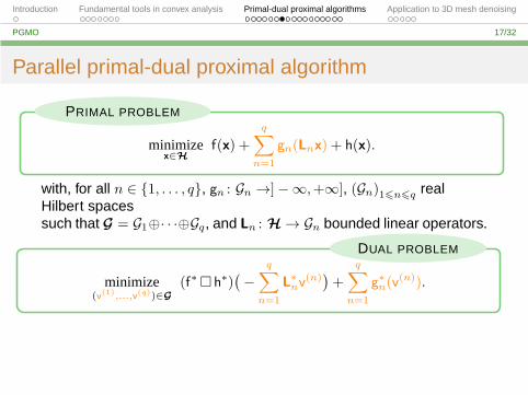
Parallel primal-dual proximal algorithm

minimizex∈H

f(x) + g(Lx) + h(x).

PRIMAL PROBLEM


PGMO 17/32


minimizex∈H

f(x) +

q∑

n=1

gn(Lnx) + h(x).

PRIMAL PROBLEM

with, for all n ∈ {1, . . . , q}, gn : Gn →]−∞,+∞], (Gn)16n6q realHilbert spacessuch that G = G1⊕· · ·⊕Gq, and Ln : H → Gn bounded linear operators.


PGMO 17/32


minimizex∈H

f(x) +

q∑

n=1

gn(Lnx) + h(x).

PRIMAL PROBLEM


minimize(v(1),...,v(q))∈G

(f∗ � h∗)(−

q∑

n=1

L∗nv

(n))+

q∑

n=1

g∗n(v(n)).

DUAL PROBLEM


PGMO 17/32


minimizex∈H

f(x) +

q∑

n=1

gn(Lnx) + h(x).

PRIMAL PROBLEM


minimize(v(1),...,v(q))∈G

(f∗ � h∗)(−

q∑

n=1

L∗nv

(n))+

q∑

n=1

g∗n(v(n)).

DUAL PROBLEM

The separability of g∗ implies that proxg∗ can be obtained by computing inparallel the proximal operators of functions (g∗n)16n6q

⇒ PARALLEL PRIMAL-DUAL SCHEMES .


PGMO 18/32


for k = 0, 1, . . .

yk = proxW−1,f

(xk −W

(∇h(xk) + ck +

q∑

n=1

L∗nv(n)k

))+ ak

xk+1 = xk + λk(yk − xk)for n = 1, . . . , q⌊

u(n)k = prox

U−1n ,g∗n

(v(n)k + UnLn(2yk − xk)

)+ b

(n)k

v(n)k+1 = v

(n)k + λk(u

(n)k − v

(n)k )


PGMO 19/32

Bibliographical remarks

⋆ Pioneering work: Arrow-Hurwicz-Uzawa method for saddlepoint problems [Arrow et al. - 1958] [Nedic and Ozdaglar - 2009]

⋆ Methods based on Forward-Backward iteration:• type I : [Vu - 2013][Condat - 2013]

(extensions of [Esser et al. - 2010][Chambolle and Pock - 2011])• type II: [Combettes et al. - 2014]

(extensions of [Loris and Verhoeven - 2011][Chen et al. - 2014])

⋆ Methods based on Forward-Backward-Forward iteration[Combettes and Pesquet - 2012] [Bot and Hendrich,2014]

⋆ Projection based methods[Alotaibi et al. - 2013]

⋆ ...


PGMO 20/32

Random block coordinate strategy


PGMO 21/32

Acceleration via block alternation◮ Idea: variable splitting.


PGMO 21/32

Acceleration via block alternation◮ Idea: variable splitting.

x ∈ H

x(1) ∈ H1

x(2) ∈ H2

····

x(p) ∈ Hp

H = ×pj=1Hj

H1, . . . ,Hp are separable real Hilbert spaces

g


PGMO 21/32

Acceleration via block alternation

◮ Simplifying assumption: f and h are block separable functions.

x

x(1)

x(2)

····

x(p)

=

p∑

j=1

fj(x(j))f = f


PGMO 21/32

Acceleration via block alternation◮ Simplifying assumption: f and h are block separable functions.

x

x(1)

x(2)

····

x(p)

=

p∑

j=1

hj(x(j))

(∀j ∈ {1, . . . , p}) hj βj-Lipschitz differentiable with βj ∈ ]0,+∞[.

h = h


PGMO 22/32

Acceleration via block alternation

⋆ For each iteration k ∈ N, update a subset of components(∼ Gauss-Seidel methods).

ADVANTAGES:

X Reduced computational cost per iteration,

X Reduced memory requirement,

X More flexibility.


PGMO 23/32

Primal-dual problem

Let F the set of solutions to the problem

minimizex(1)∈H1,...,x

(p)∈Hp

p∑

j=1

(fj(x

(j)) + hj(x(j))

)+

q∑

n=1

gn

( p∑

j=1

Ln,jx(j)

)

PRIMAL PROBLEM

(∀j ∈ {1, . . . , p})(∀n ∈ {1, . . . , q})

◮ Hj and Gn separable real Hilbert spaces,

◮ fj : Hj →]−∞,+∞]

◮ hj : Hj → R βj-Lipschitz differentiable, with βj ∈ ]0,+∞[

◮ gn : Gn →]−∞,+∞]

◮ Ln,j : Hj → Gn linear and bounded,

◮ Ln ={j ∈ {1, . . . , p}

∣∣ Ln,j 6= 0}6= ∅, et L∗

j ={n ∈ {1, . . . , q}

∣∣ Ln,j 6= 0}6= ∅.


PGMO 23/32

Primal-dual problem

Let F the set of solutions to the problem

minimizex(1)∈H1,...,x

(p)∈Hp

p∑

j=1

(fj(x

(j)) + hj(x(j))

)+

q∑

n=1

gn

( p∑

j=1

Ln,jx(j)

)

PRIMAL PROBLEM

Let F∗ the set of solutions to the problem

minimizev(1)∈G1,...,v

(q)∈Gq

p∑

j=1

(f∗j � h∗j )(−

q∑

n=1

L∗n,jv(n)

)+

q∑

n=1

(g∗n(v

(n)))

DUAL PROBLEM

◮ Assume that there exists (x(1), . . . , x(p)) ∈ H1 × . . .×Hp such that

(∀j ∈ {1, . . . , p}) 0 ∈ ∂fj(x(j)) +∇hj(x

(j)) +

q∑

n=1

L∗n,j∂gn(Ln,jx

(j)).

GOAL: Find an F× F∗-valued random variable (x, v) .


PGMO 24/32

Random block coordinate primal-dual proximal algorithm

For k = 0, 1, . . .

for j = 1, . . . , p⌊y(j)k = ε

(j)k

(proxW

−1j

,fj

(x(j)k −Wj(∇hj(x

(j)k ) + c

(j)k +

∑q

n=1 L∗n,jv

(n)k )

)+ a

(j)k

)

x(j)k+1 = x

(j)k + λkε

(j)k (y

(j)k − x

(j)k )

for n = 1, . . . , qu(n)k = ε

(p+n)k

(proxU

−1n ,g∗n

(v(n)k + Un

p∑

j=1

Ln,j(2y(j)k − x

(j)k )

)+ b

(n)k

)

v(n)k+1 = v

(n)k + λkε

(p+n)k (u

(n)k − v

(n)k ),

(εk)k∈N is a vector of p+ q Boolean variables randomly chosen at eachiteration k ∈ N in order to signal the primal and dual blocks to be updated.


PGMO 25/32


Assume that

◮ The variables (εk)k∈N are independent and identically distributed, suchthat for every k ∈ N, (∀n ∈ {1, . . . , q}) P[ε

(p+n)k = 1] > 0, and

(∀j ∈ {1, . . . , p}) ε(j)k = max

16n6q

{ε(p+n)k

∣∣ n ∈ L∗j

},


PGMO 25/32


Assume that

◮ The variables (εk)k∈N are independent and identically distributed, suchthat for every k ∈ N, (∀n ∈ {1, . . . , q}) P[ε

(p+n)k = 1] > 0, and

(∀j ∈ {1, . . . , p}) ε(j)k = max

16n6q

{ε(p+n)k

∣∣ n ∈ L∗j

},

◮ (∀j ∈ {1, . . . , p}) Wj ∈ S+(Hj), (∀n ∈ {1, . . . , q}) Un ∈ S+(Gn), with

1−(∑p

j=1

∑qn=1 ‖U

1/2n Ln,jW

1/2j ‖2

)1/2

> 12max{(‖Wj‖βj)16j6p},

◮ (∀k ∈ N) λk ∈ ]0, 1] and infk∈N λk > 0,

◮∑

k∈N

√E‖ak‖2 < +∞,

∑

k∈N

√E‖bk‖2 < +∞, and

∑

k∈N

√E‖ck‖2 < +∞ a.s.

◮ (xk)k∈N converges weakly a.s. to an F-valued random variable.

◮ (vk)k∈N converges weakly a.s. to an F∗-valued random variable.

Proof: Based on properties of quasi-Fejér stochastic sequences[Combettes & Pesquet – 2015].


PGMO 26/32

Illustration of the random sampling strategyBlock selection (∀k ∈ N)

x(1)k activated when ε(1)k = 1






How to choose (∀k ∈ N) thevariable εk = (ε

(1)k , . . . , ε

(6)k )?


PGMO 26/32









(1)k , . . . , ε

(6)k )?

P[εk = (1, 1, 0, 0, 0, 0)] = 0.1


PGMO 26/32

Illustration of the random sampling strategyBlock selection (∀n ∈ N)








(1)k , . . . , ε

(6)k )?

P[εk = (1, 1, 0, 0, 0, 0)] = 0.1

P[εk = (1, 0, 1, 0, 0, 0)] = 0.2


PGMO 26/32









(1)k , . . . , ε

(6)k )?

P[εk = (1, 1, 0, 0, 0, 0)] = 0.1

P[εk = (1, 0, 1, 0, 0, 0)] = 0.2

P[εk = (1, 0, 0, 1, 1, 0)] = 0.2


PGMO 26/32









(1)k , . . . , ε

(6)k )?

P[εk = (1, 1, 0, 0, 0, 0)] = 0.1

P[εk = (1, 0, 1, 0, 0, 0)] = 0.2

P[εk = (1, 0, 0, 1, 1, 0)] = 0.2

P[εk = (0, 1, 1, 1, 1, 1)] = 0.5


PGMO 27/32

Extension to distributed algorithms ...

Find an element of the set F of the solutions to

minimizex∈H

m∑

i=1

fi(x) + hi(x) + gi(Mix)

OPTIMIZATION PROBLEM

with H,G1, . . . ,Gm separable Hilbert spaces and, for all i ∈{1, . . . ,m}:

◮ hi βi-Lipschitz differentiable with βi ∈ ]0,+∞[,◮ Mi : H → Gi non-zero linear and bounded operators.


PGMO 27/32

Extension to distributed algorithms ...

Find an element of the set F of the solutions to

minimizex∈H

m∑

i=1

fi(x) + hi(x) + gi(Mix)


m

Find (x1, . . . , xm) ∈ Hm such that

minimize(xi)16i6m∈Λm

m∑

i=1

fi(xi) + hi(xi) + gi(Mixi)

with Λm ={(xi)16i6m ∈ Hm

∣∣ x1 = . . . = xm}



PGMO 28/32

3D mesh denoising

(ANR GRAPHSIP)

Original mesh x Observed mesh z

Undirected nonreflexive graph

OBJECTIVE: Estimate x = (xi)16i6M from noisy observationsz = (zi)16i6M where, for every i ∈ {1, . . . ,M}, xi ∈ R

3 is thevector of 3D coordinates of the i-th vertex of a mesh

⋆ H = (R3)M


PGMO 28/32

3D mesh denoising(ANR GRAPHSIP)

OBJECTIVE: Estimate x = (xi)16i6M from noisy observationsz = (zi)16i6M where, for every i ∈ {1, . . . ,M}, xi ∈ R

3 is thevector of 3D coordinates of the i-th vertex of a mesh

COST FUNCTION:

Φ(x) =

M∑

j=1

ψj(xj − zj) + ιCj (xj) + ηj‖(xj − xi)i∈Nj‖1,2

where (∀j ∈ {1, . . . ,M}),⋆ ψj : R

3 → R: ℓ2 − ℓ1 Huber function• robust data fidelity measure• convex, Lipschitz differentiable function

⋆ Cj : nonempty convex subset of R3

⋆ Nj : neighborhood of j-th vertex⋆ (ηj)16j6M : nonnegative regularization constants.


PGMO 28/32

3D mesh denoising(ANR GRAPHSIP)

OBJECTIVE: Estimate x = (xi)16i6M from noisy observations z = (zi)16i6M

where, for every i ∈ {1, . . . ,M}, xi ∈ R3 is the vector of 3D coordinates of the i-th

vertex of a mesh

COST FUNCTION:

Φ(x) =M∑

j=1

ψj(xj − zj) + ιCj(xj) + ηj‖(xj − xi)i∈Nj

‖1,2

IMPLEMENTATION DETAILS: a block ≡ a vertex

p = q =M

(∀j ∈ {1, . . . ,M})

⋆ hj = ψj(· − zj)

⋆ fj = ιCj

(∀k ∈ {1, . . . ,M})(∀x ∈ R3M )

⋆ gk(Lkx) = ‖(xk − xi)i∈Nk‖1,2


PGMO 29/32

Simulation results

⋆ positions of the original mesh are corrupted through an additive i.i.d.zero-mean Gaussian mixture noise model.

⋆ a limited number r of variables can be handled at each iteration, wherep∑

j=1

εj,n = r 6 p.

⋆ mesh decomposed into p/r non-overlapping sets.

Original mesh, M = 100250. Noisy mesh, MSE = 2.89× 10−6.


PGMO 29/32

Simulation results

Proposed reconstruction Laplacian smoothing

MSE = 8.09× 10−8 MSE = 5.23× 10−7


PGMO 30/32

Complexity

100

101

102

103

5150300

600

1200

2400

Tim

e(s.)

p/r

50

55

60

65

70

Mem

ory

(Mb)

⋆ dashed line: required memory

⋆ continuous line: reconstruction time


PGMO 31/32

Conclusion

Primal-dualproximal

algorithms

X Resolu-tion of (non)

smoothconvex

optimizationproblems

Simple

handling of

contraints

No inversion

of linear

operators

X Block-coordinatestrategies

Flexibility in

the random

selection of

primal/dual

components

Distributed

versions of

the algorithms

available

X Provenefficiencyin somesignal/image

processingapplications

X Provenconver-

gence androbustnessto errors


PGMO 32/32

Some references ...F. Abboud, E. Chouzenoux, J.-C. Pesquet, J.-H. Chenot and L. Laborelli

A Dual Block Coordinate Proximal Algorithm with Application to Deconvolution of Interlaced Video SequencesIEEE International Conference on Image Processing (ICIP 2015), 5 p., Québec, Canada, 27-30 Sep. 2015.

G. Chierchia, N. Pustelnik, B. Pesquet-Popescu and J.-C. Pesquet

A Non-Local Structure Tensor Based Approach for Multicomponent Image Recovery ProblemsIEEE Transaction on Image Processing, 23(12), pp. 5531 - 5544, Dec. 2014.

P. L. Combettes and J.-C. Pesquet

Proximal Splitting methods in Signal Processingin Fixed-Point Algorithms for Inverse Problems in Science and Engineering, H. H. Bauschke, R. Burachik, P. L.Combettes, V. Elser, D. R. Luke, and H. Wolkowicz editors. Springer-Verlag, New York, pp. 185-212, 2011.

P. L. Combettes, L. Condat, J.-C. Pesquet, and B. C. Vu

A Forward-Backward View of Some Primal-Dual Optimization Methods in Image RecoveryIEEE International Conference on Image Processing (ICIP 2014), 5 p., Paris, France, Oct. 27-30, 2014.

P. Combettes and J.-C Pesquet

Stochastic Quasi-Fejér Block-Coordinate Fixed Point Iterations with Random SweepingSIAM Journal on Optimization, 25(2), pp. 1221-1248, 2015.

A. Florescu, E. Chouzenoux, J.-C. Pesquet, P. Ciuciu and S. Ciochina

A Majorize-Minimize Memory Gradient Method for Complex-Valued Inverse ProblemsSignal Processing, 103, pp. 285-295, 2014.

A. Jezierska, E. Chouzenoux, J.-C. Pesquet and H. Talbot

A Convex Approach for Image Restoration with Exact Poisson-Gaussian Likelihoodto appear in SIAM Journal in Imaging Sciences, 2015.

N. Komodakis and J.-C. Pesquet

Playing with Duality: An Overview of Recent Primal-Dual Approaches for Solving Large-Scale OptimizationProblemsto appear in IEEE Signal Processing Magazine, 2015.

J.-C. Pesquet and A. Repetti

A Class of Randomized Primal-Dual Algorithms for Distributed Optimizationto appear in Journal of Nonlinear and Convex Analysis, 2015.

A. Repetti, E. Chouzenoux and J.-C. Pesquet

A Random Block-Coordinate Primal-Dual Proximal Algorithm with Application to 3D Mesh DenoisingIEEE International Conference on Acoustics, Speech, and Signal Processing (ICASSP 2015), 5 p., Brisbane,Australia, Apr. 19-24, 2015.

Date post:	05-May-2018
Category:	Documents
Upload:	ngotu
View:	215 times
Download:	3 times

An Overview of Recent and Brand New Primal-Dual Methods ... · An Overview of Recent and Brand New...

Documents