Lab Assignment #3

Analog Modulation (An Introduction to RF Signal, Noise and Distortion Measurements in the Frequency Domain) By: Timothy X Brown, Olivera Notaros, Nishant Jadhav

TLEN 5320 Wireless Systems Lab University of Colorado, Boulder

Purpose This lab is intended to be a beginning tutorial on Analog Modulation. It is written for those who are unfamiliar with spectrum analyzers, and would like a basic understanding of how they work, what you need to know to use them to their fullest potential, in signal, noise and distortion measurements. It is written for university level engineering students, therefore a basic understanding of electrical concepts is recommended. Equipment: • Agilent ESG-D4000A signal generator

• Agilent ESA-L1500A spectrum analyzer

Pre-Study:

How can we measure electrical signals in a circuit to help us determine the overall system performance? First, we need a “passive” receiver, meaning it doesn’t do anything to the signal under test. I just displays it in a way that makes it easy to analyze the signal, without masking the signals true characteristics. The receiver most often used to measure these signals in the time domain is an oscilloscope. In the frequency domain, the receiver of choice is called a spectrum analyzer. Spectrum analyzers usually display raw, unprocessed signal information such as voltage, power, period, waveshape, sidebands, and frequency. They can provide you with a clear and precise window into the frequency spectrum.

1

Depending upon the application, a signal could have several different characteristics. For example, in communications, in order to send information such as your voice or data, it must be modulated onto a higher frequency carrier. A modulated signal will have specific characteristics depending on the type of modulation used. When testing non-linear devices such as amplifiers or mixers, it is important to understand how these create distortion products and what these distortion products look like. Understanding the characteristics of noise and how a noise signal looks compared to other types of signals can also help you in analyzing your device/system. Understanding the important aspects of a spectrum analysis for measuring all of these types of signals will give you greater insight into your circuit or systems true characteristics.

Traditionally, when you want to look at an electrical signal, you use an oscilloscope to see how the signal varies with time. This is very important information; however, it doesn’t give you the full picture. To fully understand the performance of your device/system, you will also want to analyze the signal(s) in the frequency-domain. This is a graphical representation of the signal’s amplitude as a function of frequency The spectrum analyzer is to the frequency domain as the oscilloscope is to the time domain. (It is important to note that spectrum analyzers can also be used in the fixed-tune mode (zero span) to provide time-domain measurement capability much like that of an oscilloscope.) The figure shows a signal in both the time and the frequency domains. In the time domain, all frequency components of the signal are summed together and displayed. In the frequency domain, complex signals (that is, signals composed of more than one frequency) are separated into their frequency components, and the level at each frequency is displayed. Frequency domain measurements have several distinct advantages. For example, let’s say you’re looking at a signal on an oscilloscope that appears to be a pure sine wave. A pure sine wave has no harmonic distortion. If you look at the signal on a spectrum analyzer, you may find that your signal is actually made up of several frequencies. What was not discernible on the oscilloscope becomes very apparent on the spectrum analyzer. Some systems are inherently frequency domain oriented. For example, many telecommunications systems use what is called Frequency Division Multiple Access (FDMA) or Frequency Division Multiplexing (FDM). In these systems, different users are assigned different frequencies for transmitting and receiving, such as with a cellular phone. Radio stations also use FDM, with each station in a given geographical area occupying a particular frequency band. These types of systems must be analyzed in the frequency domain in order to make sure that no one is interfering with users/radio stations on neighboring frequencies. We shall also see later how measuring with a frequency domain analyzer can greatly reduce the amount of noise present in the measurement because of its ability to narrow the measurement bandwidth. From this view of the spectrum, measurements of frequency, power, harmonic

2

content, modulation, spurs, and noise can easily be made. Given the capability to measure these quantities, we can determine total harmonic distortion, occupied bandwidth, signal stability, output power, intermodulation distortion, power bandwidth, carrier-to-noise ratio, and a host of other measurements, using just a spectrum analyzer.

The most common measurements made using a spectrum analyzer are: modulation, distortion, and noise. Measuring the quality of the modulation is important for making sure your system is working properly and that the information is being transmitted correctly. Understanding the spectral content is important, especially in communications where there is very limited bandwidth. The amount of power being transmitted (for example, to overcome the channel impairments in wireless systems) is another key measurement in communications. Tests such as modulation degree, sideband amplitude, modulation quality, occupied bandwidth are examples of common modulation measurements. In communications, measuring distortion is critical for both the receiver and transmitter. Excessive harmonic distortion at the output of a transmitter can interfere with other communication bands. The pre-amplification stages in a receiver must be free of intermodulation distortion to prevent signal crosstalk. An example is the intermodulation of cable TV carriers that moves down the trunk of the distribution system and distorts other channels on the same cable. Common distortion measurements include intermodulation, harmonics, and spurious emissions. Noise is often the signal you want to measure. Any active circuit or device will generate noise. Tests such as noise figure and signal-to-noise ratio (SNR) are important for characterizing the performance of a device and/or its contribution to overall system noise. For all of these measurements, it is important to understand the capabilities and limitiations of your test equipment for your specific requirements. It is the goal of this lab to familiarize the student with the most important fundamental concepts in spectrum analysis and their applications in circuit design, verification and troubleshooting.

3

Amplitude Modulation

Amplitude modulation occurs when a modulating signal, fmod

, causes an instantaneous amplitude deviation of the modulated carrier. The amplitude deviation is proportional to the instantaneous amplitude of f

mod. The rate of deviation is proportional to the frequency of f

mod.

The AM modulation index, m, is defined as: m = 2 x Vsideband ÷ V

carrier . Percent AM = 100 x m. By letting the modulating waveform be represented by cos(wmt), we can describe this signal in the frequency domain as three sine waves: v(t) = [1 + m x cos(w

m x t)] x cos(w

c x t) = cos(w

c x t) + m/2 x cos[(w

c- w

m)x t] + m/2 x cos[(w

c+ w

m) x t]

4

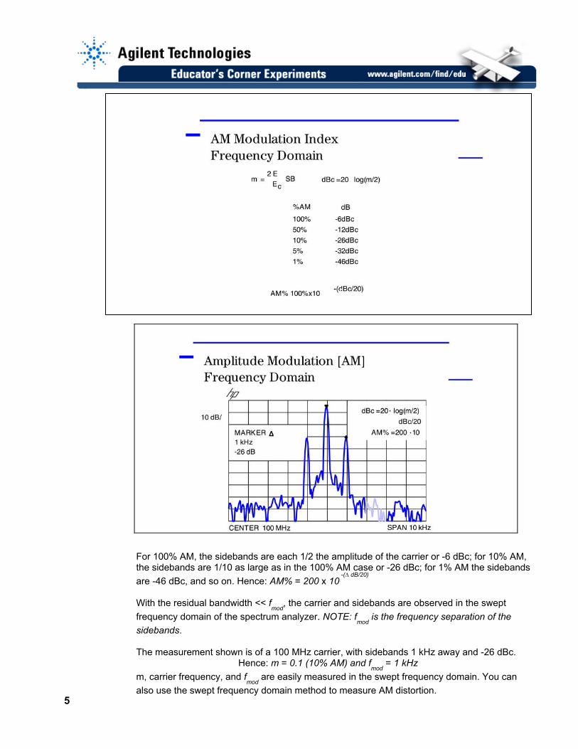
For 100% AM, the sidebands are each 1/2 the amplitude of the carrier or -6 dBc; for 10% AM, the sidebands are 1/10 as large as in the 100% AM case or -26 dBc; for 1% AM the sidebands are -46 dBc, and so on. Hence: AM% = 200 x 10 -(∆ dB/20)

With the residual bandwidth << f

mod, the carrier and sidebands are observed in the swept

frequency domain of the spectrum analyzer. NOTE: fmod

is the frequency separation of the sidebands. The measurement shown is of a 100 MHz carrier, with sidebands 1 kHz away and -26 dBc. Hence: m = 0.1 (10% AM) and f

mod = 1 kHz

m, carrier frequency, and fmod are easily measured in the swept frequency domain. You can

also use the swept frequency domain method to measure AM distortion. 5

The purpose of this lab is to familiarize the users with the RF signal generator’s modulation generation and RF spectrum analyzer’s modulation analysis capability. This section of the lab will cover AM modulation and analysis. Configure the signal generator and spectrum analyzer to create and view an AM modulated signal with a f

mod = 10 kHz

Instruction Keystroke Return the ESG-D4000A to a known state [Preset] Select an output frequency [Frequency][300][kHz] Select output signal level [Amplitude][-10][dBm] Configure modulation output [AM][AM Depth][10%] Set modulation rate and enable modulation [AM Rate][10 kHz][AM On] Enable RF output [RF On/Off] Once the signal generator has been configured, set up the spectrum analyzer to display the generated signal, by connecting the RF output of the signal generator to the RF input of the spectrum analyzer and following the instructions below. Instruction Keystroke Return the ESA-L1500A to a known state [Preset] Select a frequency range to display [Frequency][Center Freq][300][kHz] [Span][50][kHz] Select the minimum resolution bandwidth [BW/Avg][1 kHz] available on the signal analyzer Measure and record the 10 kHz AM sideband [Marker] level of the 300 kHz carrier. [Peak Search] Use RPG knob to move delta marker [Marker Delta] to one of the 10 kHz sidebands and record the marker value below. @ 310 kHz Delta dB = __________ dBc Calculate the %AM associated with the dBc value that you read on the spectrum

analyzer using the following equation. %AM Modulation Index = m = 2 * 10 exp(Delta dB/20) * 100% %AM Modulation Index = m = __________ Re-configure modulation output of the [AM][AM Rate][1 kHz] signal generator so that fmod = 1 kHz Remeasure and recalculate the signal’s %AM for the new signal fmod = 1 kHz @ 301 kHz Delta dB = __________ dBc %AM Modulation Index = m = __________ Why does this calculated value not agree with value that you set on the signal generator? Hint: The minimum resolution BW on the Agilent ESA-L1500A is 1 kHz.

Re-configure modulation output of the signal generator so that f

mod = 10 kHz and remeasure

the signal under test’s %AM using the spectrum analyzer’s built-in %AM function Re-configure modulation output of the [AM][AM Rate][10 kHz]

signal generator so that f

mod = 10 kHz 6

Instruction Keystroke Return the ESA-L1500A to a known state [Preset] Select a frequency range to display [Frequency][Center Freq][300][kHz] [Span][50][kHz]

Select the minimum resolution bandwidth [BW/Avg][1 kHz] available on the signal analyzer

Activate the automatic %AM function [Measure][%AM On] %AM Modulation Index = m = __________

The three terms in the equation given at the beginning of this section of the lab can be represented by three rotating vectors. One is the carrier term, spinning at the carrier frequency. The upper sideband is represented by a vector that is spinning at a higher rate than the carrier, and the lower sideband is represented by a vector spinning at a lower rate. The three vectors add vectorially in the time domain to form the single modulated signal, which we see here. To be in the time domain, the resolution bandwidth of our instrument must be wider than the spectral components.

7

It was mentioned briefly that although a spectrum analyzer is primarily used to view signals in the frequency domain, it is also possible to use the spectrum analyzer to look at the time domain. This is done with a feature called zero-span. This is useful for determining modulation type or for demodulation. The spectrum analyzer is set for a frequency span of zero (hence the term zero-span) with some nonzero sweep time. The center frequency is set to the carrier frequency and the resolution bandwidth must be set large enough to allow the modulation sidebands to be included in the measurement. The analyzer will plot the amplitude of the signal versus time, within the limitations of its detector and video and RBWs. A spectrum analyzer can be thought of as a frequency selective oscilloscope with a BW equal to the widest RBW. The previous slide is showing us an amplitude modulated signal using zero-span. The display is somewhat different than that of an oscilloscope: Since the spectrum analyzer does not display negative voltages, we only see the upper half of the time domain representation. Also, the spectrum analyzer uses envelope detectors, which strip off the carrier. Hence, only the baseband modulating signal is seen. The display shows a ∆ marker 10 ms. Since this is the time between two peaks, the period T is 10 milli-seconds. Recall: Period T = 1/f

mod. Hence: f

mod is 100 Hz.

8

The first formula can be used to calculate m, just like an oscilloscope. However, use the second formula when using the spectrum analyzer’s relative markers. Relative markers in linear mode show the ratio. For example, if the relative marker reads “0.1x”, this means that the lower signal is “0.1 times” or 10% of voltage of the higher signal. Configure the signal generator for the measurement of %AM using the 0 span (time domain) method on the spectrum analyzer. Instruction Keystroke Return the ESG-D4000A to a known state [Preset] Select an output frequency [Frequency][100][MHz] Select output signal level [Amplitude][-10][dBm] Configure modulation output [AM][AM Depth][30%] Set modulation rate and enable modulation [AM Rate][100 Hz][AM On] EnableRF output [RF On/Off] Configure the spectrum analyzer to measure %AM using the 0 span (time domain) method. Instruction Keystroke Return the ESA-L1500A to a known state [Preset] Select a frequency range to display [Frequency][Center Freq][100][MHz] [Span][0][kHz] Select a linear amplitude display [Amplitude][Scale Type Lin] Select the minimum resolution bandwidth [BW/Avg][1 kHz]

available on the signal analyzer Set the x-axis (time) resolution of the [Sweep][Sweep Time][150][msec] spectrum analyzer Put the analyzer in single sweep mode [Single Sweep] to freeze a trace in time Use the delta marker search functions to find Emax/Emin value, to calculate the signals %AM. Note: In linear amplitude mode, the delta marker between Emax & Emin will automatically read out the ratio Emax/Emin. Period T = 1/fmod

= _______________ f

mod = _______________

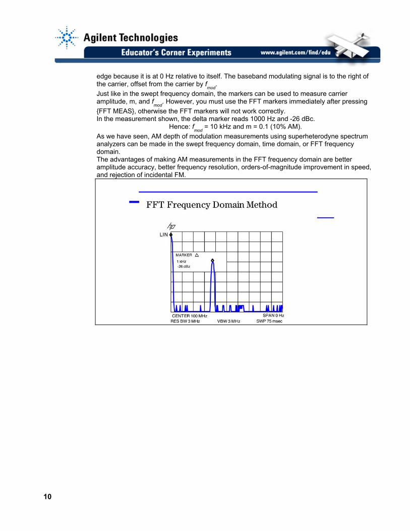
Emax/Emin = _______________ Emin/Emax = _______________ %AM = _______________ With some spectrum analyzers it is also possible to measure %AM using an FFT function. This function gives an FFT frequency domain display relative to the carrier. The carrier is at the left

9

edge because it is at 0 Hz relative to itself. The baseband modulating signal is to the right of the carrier, offset from the carrier by f

mod.

Just like in the swept frequency domain, the markers can be used to measure carrier amplitude, m, and f . However, you must

mod{FFT MEAS}, otherwise the FFT markers will not work correctly. In the measurement shown, the delta marker reads 1000 Hz and -26 dBc. Hence: f = 10 kHz and m = 0.1 (10% A

use the FFT markers immediately after pressing

M). odyne spectrum

r FFT frequency

accuracy, better frequency resolution, orders-of-magnitude improvement in speed,

modAs we have seen, AM depth of modulation measurements using superheteranalyzers can be made in the swept frequency domain, time domain, odomain. The advantages of making AM measurements in the FFT frequency domain are better amplitudeand rejection of incidental FM.

10

AM Measurement Method Selection Guide for Spectrum Analyzers Meas Method Accuracy fmod m

m Swept Frequency Domain (narrow Res BW) Log Fidelity > (Shape Factor/2) Res BW

Sinusoidal > ≈.002

m Time Domain (wide Res BW) Linearity

(1/STmax

) < fmod

< (N/2)/ST min Sinusoidal

> ≈.01

m FFT Frequency Domain (wide Res BW)

± 0.2 dB

.02 · N/(2 · ST)max

) <fmod < N/(2 · ST

min)

Sinusoidal > ≈.002

Swept Frequency Domain Method - The swept frequency domain is the method of choice for best absolute and relative frequency accuracy (e.g.; measuring f

mod ). Time Domain Method - Only spectrum analyzers without the FFT need to use the time domain method. This method is less accurate and less sensitive to low % AM. However, it is useful for voice or noise modulation. FFT Frequency Domain Method - Even a low-cost spectrum analyzer can make the most accurate AM measurements using this method. This is the method of choice for economy or mid-performance or high-performance spectrum analyzers for f

mod < 5 kHz (approximately).

Terminology of Amplitude Modulation fmod Frequency of modulation, modulation rate T Period of modulation fc Carrier frequency m Modulation index, modulation depth %AM Percent amplitude modulation, modulation depth

What is FM? Frequency modulation occurs when a modulating signal, f

mod, causes an

instantaneous frequency deviation of the modulated carrier. The peak frequency deviation, ∆ fpeak

, is proportional to the instantaneous amplitude of fmod

. The rate of deviation is proportional to the frequency of f

mod. 11

The FM modulation index, ß, is defined as ß = ∆ fpeak

/fmod

in radians, and equals the peak phase deviation.

FM is composed of an infinite number of sidebands. However, in the narrowband FM* case, there are only two significant sidebands, whose amplitude with respect to the carrier are: dBc = 20 log (ß/2). Therefore, the modulation index is: ß = 2 x 10 (dBc/20)

(This is called the “narrowband formula”). Note: f

mod is the frequency separation of the sidebands, which may be measured to counter

accuracy, and ∆ fpeak

= ß x fmod

. Hence: ß, ∆ fpeak

, fmod

, and the carrier frequency are easily measured in the narrow band case.

12

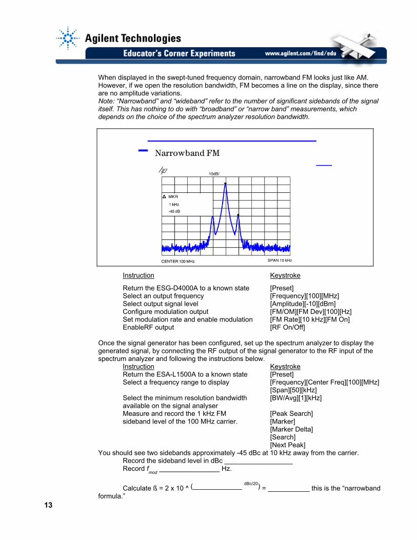
When displayed in the swept-tuned frequency domain, narrowband FM looks just like AM. However, if we open the resolution bandwidth, FM becomes a line on the display, since there are no amplitude variations. Note: “Narrowband” and “wideband” refer to the number of significant sidebands of the signal itself. This has nothing to do with “broadband” or “narrow band” measurements, which depends on the choice of the spectrum analyzer resolution bandwidth.

Instruction Keystroke

Return the ESG-D4000A to a known state [Preset] Select an output frequency [Frequency][100][MHz] Select output signal level [Amplitude][-10][dBm] Configure modulation output [FM/OM][FM Dev][100][Hz] Set modulation rate and enable modulation [FM Rate][10 kHz][FM On] EnableRF output [RF On/Off] Once the signal generator has been configured, set up the spectrum analyzer to display the generated signal, by connecting the RF output of the signal generator to the RF input of the spectrum analyzer and following the instructions below. Instruction Keystroke Return the ESA-L1500A to a known state [Preset] Select a frequency range to display [Frequency][Center Freq][100][MHz] [Span][50][kHz]

Select the minimum resolution bandwidth [BW/Avg][1][kHz] available on the signal analyser

Measure and record the 1 kHz FM [Peak Search] sideband level of the 100 MHz carrier. [Marker] [Marker Delta] [Search] [Next Peak] You should see two sidebands approximately -45 dBc at 10 kHz away from the carrier. Record the sideband level in dBc __________________ Record f

mod Hz.

Calculate ß = 2 x 10 ^ ( dBc/20) = this is the “narrowband formula.”

13

Calculate ∆ fpeak

= ß x fmod

= ∆ fpeak

= x = __________ Now increase the resolution bandwidth to 1 MHz and prove to yourself that this is not AM. The signal generator is set for b = ∆ f

peak/f

mod = 20 Hz/1000 Hz = 0.02. Note: ∆ fpeak frequency deviation << f

mod. In other words, the spectrum width is much greater

than the deviation of the carrier! That’s because the sideband spacing determines the rate at which the carrier is deviating. In our measurement, the rate of deviation is much greater than the peak frequency deviation of the carrier. Vary the FM rate and deviation on the ESG-D4000A signal generator and observe the change in the displayed signal of the spectrum analyzer.

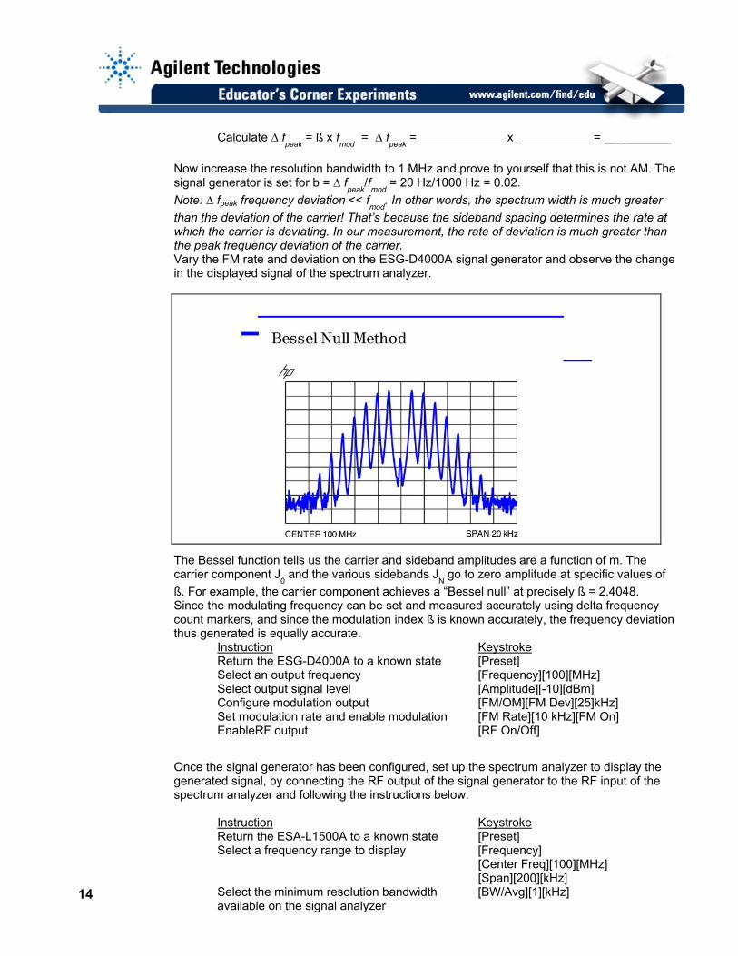
The Bessel function tells us the carrier and sideband amplitudes are a function of m. The carrier component J

0 and the various sidebands J

N go to zero amplitude at specific values of

ß. For example, the carrier component achieves a “Bessel null” at precisely ß = 2.4048. Since the modulating frequency can be set and measured accurately using delta frequency count markers, and since the modulation index ß is known accurately, the frequency deviation thus generated is equally accurate. Instruction Keystroke Return the ESG-D4000A to a known state [Preset] Select an output frequency [Frequency][100][MHz] Select output signal level [Amplitude][-10][dBm] Configure modulation output [FM/OM][FM Dev][25]kHz] Set modulation rate and enable modulation [FM Rate][10 kHz][FM On] EnableRF output [RF On/Off]

Once the signal generator has been configured, set up the spectrum analyzer to display the generated signal, by connecting the RF output of the signal generator to the RF input of the spectrum analyzer and following the instructions below. Instruction Keystroke Return the ESA-L1500A to a known state [Preset] Select a frequency range to display [Frequency] [Center Freq][100][MHz] [Span][200][kHz]

Select the minimum resolution bandwidth [BW/Avg][1][kHz] available on the signal analyzer

14

15

rrier. [Peak Search]

elta] or [Next Pk Left]

ow far_____

t the first

Calculate ∆ fpeak

= ß x fmod

Measure and record the 10 kHz FM [Marker] sideband level of the 100 MHz ca

Use the next peak right or left function [Marker D to find the f and “nulled” carrier value [Next Pk Right]

mod for the modulated signal under test H has the carrier been “nulled” below the first ( ß = 2.4048) sideband = _ _______ You should see the carrier “nulled” (approximately -40 dBc, or more). Recall thacarrier null ß = 2.4048. ∆ f

peak = 2.4048 x = ______________

formula (given er) for calcu

NOTE: If there are more than two significant sidebands, the “Narrowband FM”earli lating b does not work. For more information on wideband FM analysis refer to Hewlett-Packard Company, Spectrum Analysis Basics, Application Note 150 (HP publication number 5952-0292, November 1, 1989)

ferences: Hewlett-Packard Company, Spectrum Analysis Basics

Re1. , Application Note 150 (HP

number 5952-0292, November 1, 1989) publication

2. Hewlett-Packard Company, 8 Hints to Better Spectrum Analyzer Measurements , publication number 5965-6854E, December, 1996)

(HP

3. Hewlett-Packard Company, Amplitude and Frequency Modulation, Application Note 150(HP publication number 5954-9130, January, 1989)

-1

4. Witte, Robert A., Spectrum and Network Measurements, Prentice Hall, Inc., 1993

Tthe

hese experiments have been submitted by third parties and Agilent has not tested any of the experiments. You will undertake any of experiments solely at your own risk. Agilent is providing these experiments solely as an informational facility and without review.

ANY DIRECT, INDIRECT, GENERAL, INCIDENTAL, SPECIAL OR CONSEQUENTIAL DAMAGES IN CONNECTION WITH THE USE OF ANY OF THE EXPERIMENTS.

AGILENT MAKES NO WARRANTY OF ANY KIND WITH REGARD TO ANY EXPERIMENT. AGILENT SHALL NOT BE LIABLE FOR