1

ANALYSING THE EFFECT OF TREASURY BILL RATES

ON STOCK MARKET RETURNS USING GARCH MODEL

BY

OTIENO ODHIAMBO LUTHER

AND

REGINA KALOMBE MUTOKO

2010

ABSTRACT

This paper examines the relationship between the returns of ordinary shares listed at the

Nairobi Stock Exchange (NSE) and the Treasury Bills Rate using GARCH Analysis. Existing

studies in Kenya on the relationship of factors affecting the returns of assets in the NSE have

used various methods, mostly Ordinary Least Squares (OLS) Regression and have yielded

inconclusive results. This study recognizes the unique characteristic of financial series data

that makes common analysis techniques like OLS regression unsuitable for generating

effective forecast models. The study systematically examines the returns of the various market

segment returns within the NSE for these characteristics so as to build a basis for using

GARCH analysis. Finally, it compares the results obtained using OLS regression with the

results obtained using GARCH analysis techniques.

The study concluded that in keeping with theory, Treasury Bill Rates have a significant

impact on the asset returns of the various market segments, the NSE – 20 Share Price Index

and All market returns as a whole. The behaviour of the returns of assets on the NSE can be

better explained by considering the volatility of previous periods. The study found that

GARCH analysis gives a better explanation for the relationship between Treasury Bill Rates

and asset returns than OLS regression in every market segment. Furthermore, the explanatory

power becomes stronger as we consider the effect of previous variances on the current

observations.

2

INTRODUCTION

Over the years financial analysts and investors have been concerned about the impact of

Treasury bills rate on the behavior of stock returns. Institutions that issue Treasury bills and

stocks are competing for investors‘ funds. Correct choice ensures that the investors are able to

reduce their risk and enhance returns by recognizing the underlying direction of the markets

and taking positions accordingly. This is in line with the assumption that rational investors

only assume risk if they will be adequately compensated. Therefore investors have to rank

assets on a risk- return perspective then select the assets to invest in according to their

individual risk preferences as noted by Markowitz (1952) in his mean variance paradigm.

Treasury bills are the least risky, Elton and Gruber (1995), but play a special role in financial

theory because they have no risk of default in addition to very short term maturities. Ordinary

shares issued by private entities represent an ownership claim on the earnings and assets of the

firm that issued them, Elton and Gruber (1995). Even with the limited liability that ordinary

shares come with, the residual nature of claims (on a firm‘s assets and earnings) accruing to

shareholders, this class of investment is considered the riskiest. However money to productive

sector in the form of subscription for stocks in corporations could contribute much more

desired economic growth than money invested in treasury bills.

The interest on Treasury bills is generally viewed as the representative money market rate. For

this reason Treasury bill interest rates are typically used as the index rate for variable rate

financial contracts. In particular, the spread between private money rates and Treasury bill

interest rates is used as a measure of the default risk premium on private securities. It is

therefore not surprising that the Treasury bill interest rate is generally used to test various

hypotheses about the effect of such economic variables as the rate of inflation or the money

supply on the general level of short term interest rates, Cook and Lawyer (1983). Furthermore

Treasury bill interest rates are used to test hypotheses about the determinants of money market

yield curves. Despite this central role accorded to Treasury bill interest rates, they frequently

diverge greatly from other high risk assets of comparable maturity. Furthermore, this

differential is subject to abrupt change, Cook and Lawyer, (1983).

3

Studies on financial markets and specifically those on the pricing of assets, model the

relationship between competing assets such as private stock returns and Treasury Bills using

linear regression techniques. However, a significant re-evaluation of statistical basis of

econometric models starting in the 1980s suggests that there is a need to balance theory with

statistical analysis (Banerjee, Dolado, Galbraith and Hendry, 1993). Econometric modeling

basis has expanded from assumption of stationary to include integrated processes. The effect

of the expansion is continuing and is having enormous influence on choice of model forms,

statistical inference and interpretation of a number of traditional concepts such as collinearity,

forecasting and measurement errors.

Stationary time series data showing fluctuating volatility and, in particular, financial return

series have provided the impetus for the study of a whole series of econometric time series

models that may be grouped under the general heading of GARCH (Generalized Auto

Regressive Conditionally Heteroskedastic) models, Engle (1982), Bollerslev, Chou, and

Kroner, (1992) and Shephard, (1996). The hidden variable volatility depends parametrically

on lagged values of the process and lagged values of volatility.

GARCH modeling, which builds on advances in the understanding and modeling of volatility

in the last decade, has become an important econometric technique. GARCH takes into

account excess kurtosis and volatility clustering, two important characteristics of financial

time series. It provides accurate forecasts of variances and covariances of asset returns

through its ability to model time-varying conditional variances. As a consequence, GARCH

models have been applied successfully to such diverse fields as risk management, portfolio

management and asset allocation, option pricing, foreign exchange, and the term structure of

interest rates. Highly significant GARCH effects have been found in equity markets, not only

for individual stocks, but for stock portfolios and indices, and equity futures markets as well,

Bollerslev, Chou, Kroner, (1992). These effects are important in such areas as value-at-risk

(VaR) and other risk management applications that concern the efficient.

This study examines the relationship between Treasury Bills Rate and the return of assets on

the Nairobi Stock Exchange using GARCH analysis. The study also carries out OLS linear

regression and compares their forecasting capability to those obtained through GARCH

analysis.

4

STATEMENT OF THE PROBLEM, OBJECTIVE OF THE STUDY,

JUSTIFICATION OF THE STUDY

In Kenya the bearish nature of the stock market before 2002 has been blamed on the excessive

borrowing by the Kenya Government. Jiwaji (2004), writing for G21 notes, "Kenyans have

paid and continue to pay a very high price, both in budgetary and economic costs, for the

financial indiscipline of the 1990s which was characterized by high fiscal deficits, excessive

domestic borrowing...‖ If the preceding assertion holds, then an association exists between

government borrowing and stock market performance and must be visible and capable of

adversely affecting the levels of private investment.

Economist Valentino Piana, (2002) tells us that a large and abrupt increase in general interest

rates can have devastating effects on crucial real variables, exerting a depressing pressure on

Gross Domestic Product (GDP) and the economy at large. Macroeconomic theory suggests it

is through interest rates that monetary policy actions are transmitted to the economy, Roley

and Sellon (1995). Furthermore, the CBK 15th Monetary Policy Statement, December (2004), notes

that when the the money supply increases, short-term rates drop, which stimulates activity in

interest-sensitive sectors. Studies of the determinants of output movements conducted since

the early 1980's found that when interest rates are considered, the monetary aggregates lose

most of their explanatory power, suggesting that interest rates contain important information

about future output, (Sims, 1980). However of concern to us is whether the relationship

between the returns of assets on the NSE and treasury bills rate is large enough to be relied on

by investors as an investment signal.

Studies on financial time series confirm that financial series exhibit increased conditional

variance and the use of Ordinary Least Squares Linear Regression may not be sufficient to

fully accommodate these variances and incorporate their impact into current forecast models.

It therefore becomes necessary to apply competing modeling approaches on NSE financial

time series data.

The first objective of this study is to examine the extent of the relationship between the

Treasury Bills rate and the returns of stocks traded on the Nairobi Stock Exchange. The

second objective is to compare Ordinary Least Square (OLS) regression analysis and GARCH

5

analysis in predicting the returns of assets on the NSE using Treasury Bills rate as the

independent variable.

Portfolio managers can use this study to counter-check their investment recommendations and

provide value maximization for their clients. They can also use this information to investigate

anomalies in expected returns that are not explained by the standard economic indicators as a

way to better appreciate the dynamics within the economy and improve portfolio returns.

Policy makers within the Government can use the findings within this study to better align

their fiscal and monetary policies. This study will provide incentives for greater fiscal

discipline so as to provide a stable environment for sustainable development. The ultimate

goal of a government is to improve the living conditions of people in their everyday lives.

Increasing the gross domestic product is not just a numbers game. Higher incomes mean good

food, warm houses, and hot water. They mean safe drinking water and inoculations against the

perennial plagues of humanity which in turn help to break the cycle of poverty to produce a

wealthy nation. This requires growth in real productive sector and a balance between the value

to invest in Treasury bills and the amount of funds to leave available in order to extend credit

to the economy.

LITERATURE REVIEW

LINK BETWEEN STOCK MARKET AND T-BILL RATE

Darrat and Dickens (1999) noted that interest rates lead stock returns. Various studies such as

the June 2004 study by the CFA Institute show that stocks in the US averaged greater returns

during periods of expansive monetary policy and smaller returns were realized when the

policy on interest rates was restrictive and that markets performed poorly, resulting in lower

than average returns and higher than average risk. Conversely, periods of expansive monetary

policy - when interest rates are falling, generally coincide with strong stock performance

including higher than average returns and less risk.

TREASURY BILL RATE AND CROWDING OUT EFFECT

6

In Kenya, the major purchasers of TBills tend to be financial institutions, Mukherjee (1999).

These same institutions are responsible for providing credit to individual and corporate

consumers. When financial institutions purchase of T-bills, the amount of money available for

private investment and development is curtailed and is expensive. (Girmens and Guillard, 2002)

and (Schenk, 2000). This result into the crowding out effect, i.e. an increase in interest rates

due to rising government borrowing in the money market, (Girmens and Guillard,2002),

(Ahmed and Miller, 1999).

THE ATTRACTIVENESS OF T-BILLS TO INVESTORS

Treasury bill rates are normally the lowest of rates within the economy. They are influenced

mainly by the expectations about government budget deficits, government short-term cash-

management needs, inflation, as well as overall conditions of demand and supply in the

markets for credit, Wagacha (2001), Fleming (1997), Stanton (2000). In some countries e.g.

United States, the interest paid on Treasury bills includes an inflation premium for any

expected loss of purchasing power, Kopcke and Kimball (1999). At the same time, however,

Treasury bill rates probably have only a small or no liquidity premium for holding bills

instead of cash because holders have a ready market in which to sell the bills, should they

need cash before the maturity date. Also missing from the interest rate paid on Treasury bills

is a credit-risk premium to offset the chance that the issuer might default because of the

superior credit standing of the government, Stanton (2000).

Thus given an opportunity, a risk averse investor will always opt for T-bills rather than risky

securities whenever Treasury bills offer higher returns. In fact, during turbulent financial

times, investors' increased desire for default-free assets tends to produce particularly low

interest rates on Treasury bills compared with money market instruments issued by the private

sector, Federal Reserve Bank of San Francisco (2005). This is because as the demand for T-

bills increase, their interest rate goes down.

THE STOCK EXCHANGE AS A PREDICTOR OF THE ECONOMY

Central Bank of Kenya‘s (CBK) monthly economic review reports the performance of the

Nairobi Stock Exchange (NSE) as one of the economic indicators. The report includes the

movements of the NSE-20 price index as well as percentage (%) trade turnover in securities

7

listed at the Nairobi Stock Exchange (NSE) and the performance of the 91 day Treasury bill.

This suggests that the CBK is aware of the importance of the NSE as a ―predictor‖ of the

economy and hence to some extent is aware of the association between changes in economy

and movements in the NSE 20 share index. Lawrence Kudlow, Chief Economist for CNBC,

the leading financial news television network in the world, says that ―The stock market index

signals to the government the ‗feel good‘ factor prevailing in the economy‖ Kudlow (2001).

As much as the finance ministry may want to ignore it, the performance of the stock market

right after the introduction of the budget gives an immediate feedback to the Finance Minister

about the acceptability of the budget. The NSE – 20 Index is considered effective and

representative, Odhiambo (2000).

The ―wealth effect‖ holds that stock prices lead economic activity by actually causing what

happens to the economy. Dynan and Dean (2001) argue that since fluctuations in stock prices

have a direct effect on aggregate spending, the economy can be predicted from the stock

market. When the market is rising, investors are wealthier and spend more. As a result, the

economy expands. On the other hand, if stock prices are declining, investors are less wealthy

and spend less. This results in slower economic growth.

As mentioned previously in this document students of finance and professionals within the

finance and economic sector in Kenya have been interested in the performance of assets on

the NSE and the ability to predict the same using various factors. The studies are mainly the

unpublished MBA thesis projects presented at the University of Nairobi and a few published

articles by professionals in the Institute of Policy and Research (IPAR) Kenya. Similar studies

by Njaramba (1990), Kerandi (1993), Gathoni (2002) relied on OLS regression. Akwimbi

(2003) investigated the relationship of NSE stock returns to selected market and industrial

variables. He focused on loans, interest on savings among others and concluded that there is

no significant relationship between these factors and the returns of assets on the stock

exchange. Rioba (2003) carried out a study to determine the predictability of ordinary stock

returns for selected securities listed on the NSE using recursive least squares regression. He

concluded that the predictability evidence for ordinary shares is weak and not conclusive.

The above studies yielded inconclusive evidence in predicting the returns of assets on the

NSE. This clearly indicates that practical considerations on the ground do not necessarily

8

agree with the theory of the day and compels finance scholars and professionals to explain

why there is a discrepancy between reality and theory.

The study is unique in that it utilizes an analysis model other than OLS regression to compare

returns of riskless asset against risky asset. As mentioned previously, GARCH has been

gaining huge success and popularity in academic and professional financial circles since its

introduction by Engle in 1920 and its significant enhancement by Bollerslev in 1996. The

deluge of GARCH material and its ability to capture the volatility inherent in financial data

prompted its use in this study. OLS Regression limits the variance over time to a constant

usually referred to as the ―error‖ term. The term itself ―error‖ is a misnomer as it suggests a

parameter that is captured as a ―by the way‖, yet statistic theory has shown that residuals in

financial data are rich in volatility content.

GARCH stands for Generalized Autoregressive Conditional Heteroskedasticity.

Heteroskedasticity is the time-varying variance i.e., volatility. Conditional implies a

dependence on the observations of the immediate past, and autoregressive describes a

feedback mechanism, by which past observations are incorporated into the present. GARCH

then is a mechanism by which past variances are included in the explanation of future

variances. More specifically, GARCH is a time series modeling technique by which past

variances and past variance forecasts are used to forecast future variances.

ARCH models were introduced by Engle (1982) and generalized as GARCH (Generalized

ARCH) by Bollerslev (1986). These models are widely used in various branches of

econometrics, especially in financial time series analysis, Bollerslev, Chou, and Kroner (1992)

and Bollerslev, Engle, and Nelson (1994). Estimates of asset return volatility are used to

assess the risk of many financial products. Accurate measures and reliable forecasts of

volatility are crucial for derivative pricing techniques as well as trading and hedging strategies

that arise in portfolio allocation problems.

Financial return volatility data is influenced by time dependent information flows which result

in pronounced temporal volatility clustering. These time series can be parameterized using

Generalized Autoregressive Conditional Heteroskedastic (GARCH) models. It has been found

that GARCH models can provide good in-sample parameter estimates and, when the

appropriate volatility measure is used, reliable out-of-sample volatility forecasts. Empirical

9

studies on financial time series have shown that they are characterized by increased

conditional variance following negative shocks (bad news). The distribution of the shocks has

also been found to exhibit considerable leptokurtosis. Since the standard Gaussian GARCH

model cannot capture these effects various GARCH model extensions have been developed.

On a purely statistical level, non-constant variance (heteroskedasticity) constitutes a threat to

inference as it biases the standard errors of coefficients. The standard approach to

heteroskedasticity is to employ a number of ―corrections‖ to overcome the statistical problems

involved (e.g., White 1980). However, the presence of heteroskedasticity in a model can also

indicate an underlying process that is theoretically interesting. In time series data, the

unconditional, or long run, variance from a model may be constant even though there are

periods where the variance increases substantially. These eruptions of high variance in some

periods can be indicative of contextual volatility often hypothesized to occur in financial

markets or public opinion. Mean models often fail to capture this dynamic because increases

or decreases in conditional variance do not necessarily imply a change in the expected mean

of the data.

The ARCH Specification

To develop garch ARCH model, one consider two distinct specifications—one for the

conditional mean and one for the conditional variance. In the standard GARCH (1, 1)

specification:

ttt xy ………………………………………….……. Equation 1

2

1

2

1

2

ttt …………...…………………………….…….. Equation 2

Where

ty = mean equation

2

t = conditional variance equation

= the mean

10

2

1t = News about volatility from the previous period, measured as the lag of the

squared residual from the mean equation i.e. the ARCH term.

2

1t = Last period‘s forecast variance i.e. the GARCH term

The mean equation given in (1) is written as a function of exogenous variables with an error

term. Since 2

t is the one-period ahead forecast variance based on past information, it is

called the conditional variance. The conditional variance equation specified in (2) is a function

of three terms namely the mean, the ARCH term and the GARCH term. The (1, 1) in GARCH

(1, 1) refers to the presence of a first-order GARCH term (the first term in parentheses) and a

first-order ARCH term (the second term in parentheses). An ordinary ARCH model is a

special case of a GARCH specification in which there are no lagged forecast variances in the

conditional variance equation.

This specification is often interpreted in a financial context, where an agent or trader predicts

this period‘s variance by forming a weighted average of a long term average (the constant),

the forecasted variance from last period (the GARCH term), and information about volatility

observed in the previous period (the ARCH term). If the asset return was unexpectedly large

in either the upward or the downward direction, then the trader will increase the estimate of

the variance for the next period. This model is also consistent with the volatility clustering

often seen in financial returns data, where large changes in returns are likely to be followed by

further large changes. There are two alternative representations of the variance equation that

may aid in the interpretation of the model. If we recursively substitute for the lagged variance

on the right-hand side of (2), we can express the conditional variance as a weighted average of

all of the lagged squared residuals:

1

212

1 j

jt

j

t

w

……………………………………………..…………. Equation 3

We see that the GARCH (1, 1) variance specification is analogous to the sample variance, but

that it down-weights more distant lagged squared errors.

11

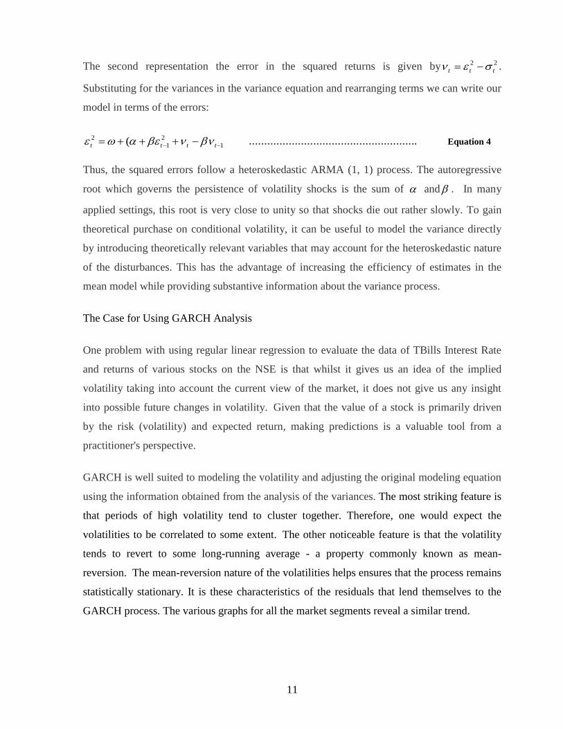
The second representation the error in the squared returns is given by 22

ttt .

Substituting for the variances in the variance equation and rearranging terms we can write our

model in terms of the errors:

1

2

1

2 ( tttt ………………………………………………. Equation 4

Thus, the squared errors follow a heteroskedastic ARMA (1, 1) process. The autoregressive

root which governs the persistence of volatility shocks is the sum of and . In many

applied settings, this root is very close to unity so that shocks die out rather slowly. To gain

theoretical purchase on conditional volatility, it can be useful to model the variance directly

by introducing theoretically relevant variables that may account for the heteroskedastic nature

of the disturbances. This has the advantage of increasing the efficiency of estimates in the

mean model while providing substantive information about the variance process.

The Case for Using GARCH Analysis

One problem with using regular linear regression to evaluate the data of TBills Interest Rate

and returns of various stocks on the NSE is that whilst it gives us an idea of the implied

volatility taking into account the current view of the market, it does not give us any insight

into possible future changes in volatility. Given that the value of a stock is primarily driven

by the risk (volatility) and expected return, making predictions is a valuable tool from a

practitioner's perspective.

GARCH is well suited to modeling the volatility and adjusting the original modeling equation

using the information obtained from the analysis of the variances. The most striking feature is

that periods of high volatility tend to cluster together. Therefore, one would expect the

volatilities to be correlated to some extent. The other noticeable feature is that the volatility

tends to revert to some long-running average - a property commonly known as mean-

reversion. The mean-reversion nature of the volatilities helps ensures that the process remains

statistically stationary. It is these characteristics of the residuals that lend themselves to the

GARCH process. The various graphs for all the market segments reveal a similar trend.

12

Lubrano (1998) notices that, when describing the transition between two regimes denoted by a

threshold, simple GARCH is ineffective. Indeed a cursory examination of time series data

shows that there are sharp transitions from positive to negative and from low values of

positive to very high values of positive. Lubrano (1998) introduced a new class of GARCH

models that allows for a smooth transition and named it STGARGH - Smooth Transition

GARCH. As financial data have very often a high frequency of observation, a smooth

transition seems a priori better than an abrupt transition. Engle and Ng (1993) found that the

most severe misspecification direction was that the tested models did not take adequately

account for the sign asymmetry. The smooth transition model addresses the problem of sign

asymmetry. It is more than a simple generalization of the TGARCH as it allows for various

transition functions that assure a great flexibility to the skedastic function, taking into account

sign but also size effects. Finally the specification retained accepts the simple GARCH as a

restriction.

Modeling Financial Returns Volatility

In this section we take a week as the unit time interval and identify return as the continuously

compounded weekly asset return tr expression for tr is then:

tr = tLog ( ) - )( 1tpLog ………..………………………..………………………… Equation 5

Where Log denotes the natural logarithm and is the asset's (close of trade) value on week t.

The weekly return volatility on week t is then

22

tt r ………..………………………..…………………………….. Equation 6

If a standard GARCH (1, 1) model is assumed then a one step-ahead out-of-sample weekly

volatility forecast can be constructed as:

2

1t = 0 + 12

t + 2

t ……………………………………..…………………….Equation 7

Where

10 bxby T

ttt …...…………………………………….….…...…. Equation 8

and

13

2

1

2

1 tt r ..……..……………………………….…………….... Equation 9

However, empirical research has shown that GARCH is not good a estimator of 2

1tr and that

much improved volatility forecasts can be obtained if high frequency (daily or intraday)

returns data are taken into account.

To be specific, if the asset price is sampled m times per day then the following

returns are generated:

)()( /1)( mtttm pLogpLogr ………………………………...….. Equation 10

Where

,/1 mt ,/2 m … Etc. and the cumulative squared returns (CSR) for day t + 1 are:

m

t

tmtm rCSR 2

1)(1)( ………………………………………...…….. Equation 11

If 1)( tmCSR is used instead of 2

1tr then standard GARCH models can provide satisfactory

volatility forecasts. In fact the quality of these forecasts has been found to increase

monotonically as the sampling frequency (m) increases.

METHODOLOGY

The study uses all the securities listed in the Nairobi Stock Exchange (NSE) as the and their

various market segments as the dependent variable and the 30-day treasury bill rate as the

independent variable. The securities are divided into various categories in order to get a

clearer picture of the impact of Treasury Bill Rate impact on the market as a whole, the

companies that constitute the NSE – 20 Share Index, and the companies that make up the

various market segments, namely Financial and Investment, Agriculture, Commercial and

Services, and Industrial.

The sample consists of securities comprising the calculation of the NSE 20 share index. The

government security is the 90-day Treasury bill. The sample is further broken down into the

various market segments in order to get a clearer understanding of the impact of the TBills

interest rate. The study is limited to the period 1996 to 2001 since data is readily available

during this period.

14

THE VARIABLES AND THEIR MEASUREMENTS

We have two assets whose return and risk we need to compute. These are stocks and the 90-

day Treasury bill. Return on Stocks and Market Index is calculated as follows:

0

10

P

DPPR i

i

……………………………………………………………. Equation 12

Where:

iR = Return on asset (stock) I; iP = Price of share (stock) at period t; 0P = Price of share

(stock) at period 1t ; and 1D = Dividend paid during the period on stock .

The above formulation will be used in calculating return on stocks that constitute NSE 20

share index on a weekly basis. The weekly frequency is dictated by the fact that T-bill interest

rates are released in most cases weekly and the fact that a larger time scale, with more

intervals of data improves the precision of estimates. The return will then be converted into

weekly annual returns to be comparable to Treasury bill rates reported by weekly by Central

Bank of Kenya.

Market Return ( mR ) is be based on NSE 20 share market index is:

n

RRRRR ntttt

m

...( 321 ………………………………………………….. Equation 13

Where:

mR = the market return; tR1 = Return on stock of the first company in week t; and

n = The number of company in the index

The calculation of returns on treasury ( tbr ) and is calculated by solving for in the following

function:

n

tb

tb

r

MVPP

)1(

……….………………………...………………………………… Equation 14

Where:

15

tbPP = Purchase price of the treasury bills; MV = Maturity value or face value of treasury

bills; tbr = The return on treasury bills; and n = The period to maturity

Stock returns variability is captured by the equation below:

T

t

t RRT 1

22 ][1

1̂ …………………………………….…………….…… Equation 15

The numbers in both sets of data are converted in their logarithms. This non-linear logarithmic

conversion of data is very useful when comparing the interest rate of T-bills with the changes

in stock prices. By converting the data into logarithms the variability becomes roughly the

same within each group (homoscedasticity) Maestas and Gleditsch (1998). Often groups that

tend to have larger values also tend to have greater within-group variability. A logarithmic

transformation will often make the within-group variability more similar across groups. This

is especially useful for the stock prices. It is also easier to describe the relationship between

the variables when it's approximately linear. Logarithmic transformations are helpful when

constructing statistical models to describe the relationship between two measurements which

in their original form seem to have no linear correlation. Finally, logarithms also play an

important role in analyzing probabilities.

Earlier studies modeled the relationship between stock returns and TBill returns using

regression analysis. Such studies overlooked the possibility that when time series data are

used in regression analysis, often the error term is not independent through time. Instead, the

errors are serially correlated or autocorrelated. If the error term is autocorrelated, the

efficiency of ordinary least-squares (OLS) parameter estimates is adversely affected and

standard error estimates are biased.

In this study, it is assumed that the error term is varying or increasing with each observation

due to the time series nature of the data. Each set of data represents a different week which

introduces its own errors into the data.

ROAD MAP OF DATA ANALYSIS

The data is put through basic data analysis to get a feel for the behaviour of the data in its raw

format and also in its transformed format.

16

1. A basic correlation analysis will be carried out on the TBills Interest Rate on an annual

basis and that of the stock returns for the various market segments. The purpose of this

analysis will be to determine if TBills Rate are independent when compared to the rate

of return of stocks. Only then can we make a decision as to whether we are dealing

with a dependent and independent variables or dealing with a case of factor analysis.

2. The second step will be to analyze the distribution of TBills Interest Rates and see

whether their distribution is linear or non-linear. The results from this step will help us

narrow down the type of data transformation that will be required at advanced stages

of the analysis.

3. The distribution of the returns of the various market segments will be undertaken to

determine if the distribution is normal. The distribution of the various market segments

will indicate whether the data needs to undergo a data transformation in order to come

up with an appropriate relationship model between rate of return and TBills Interest

Rate.

4. A test to determine whether the data is uniformly distributed will be the final

descriptive test for the data. Presence of uniform distribution is an important

assumption for carrying out various statistical tests. If the data does not have a uniform

distribution it is important that we establish this fact and seek alternative analysis

methods or transform it to obtain the desired characteristics.

5. The next step in accordance to the literature review is to establish the presence of

autoregression within the residuals of the various market segment returns. This will be

done using the Durbin Watson test and the ARCH LM Test. The Durbin-Watson test

statistic is designed for detecting errors that follow a first-order autoregressive process.

This statistic also fills an important role as a general test of model misspecification.

6. If the tests are positive for GARCH we will run ordinary linear regression and

compare the results to GARCH (1, 1) and other higher order GARCH models and test

17

to see if the GARCH estimation has a better ―goodness of fit‖ compared to OLS

regression.

7. The graphs of the various returns over time will then be analyzed to examine the

behaviour of the market segments when TBills rise and fall. The points for

examination will be generated from the TBill Graph‘s high and low points.

DATA ANALYSIS AND FINDINGS

The process of data analysis is governed by the Road Map that described above. It

starts from basic analysis of the data to determine its properties, these form the basis

for the various analysis that the data will be subjected to during the analysis stage. The

analysis then graduates to more specific analysis of graphs, which gives us a better feel

for the behaviour of the data not only in general but across certain time periods.

Finally the data is subjected to OLS Linear Regression and GARCH regression and the

results are obtained. The comparison of these two analysis techniques forms the final

part of the analysis as we examine the best fit model for each market sector.

Table 1 LEGEND OF ABBREVIATIONS USED IN THE DATA ANALYSIS

AllRetnA Returns for the entire Nairobi Stock Exchange taken on an annual basis

AgrRetA Returns for the Agricultural Market Segment taken on an annual basis

ComRetA Returns for the Commercial and Services Segment taken on an annual

basis

FinRetA Returns for the Financial and Investment Segment taken on an annual

basis

IndRetA Returns for the Industrial and Allied Segment taken on an annual basis

TBills R Returns for the Treasury Bills taken on an annual basis

NSEIRetA Returns for the for the NSE – 20 Share Price Index taken on an annual

18

basis

Table 4.1

CORRELATION ANALYSIS The null hypothesis in this case states that there is no correlation

Ho: = 0

And the alternative hypothesis states that there is a correlation

H1: < > 0

p - value < 0.05 there is evidence to support correlation; p - value > 0.05 there is evidence to

support no correlation. If a strong correlation exists, then the analysis shifts to factor analysis as

opposed analysis of independent variables. This ensures that the analysis technique employed is

suitable for the type of data we have.

CORRELATION ANALYSIS OF THE VARIOUS MARKET SEGMENTS

A B C D E F

NSEIRetA AllRetnA AgrRetA ComRetA FinRetA IndRetA

1. AllRetnA 0.720 The p value << 0.05 and hence supports the fact that there is a strong correlation

0.000

2. AgrRetA 0.434 0.379 The p value << 0.05 and indicates there is evidence to support

correlation, albeit a weak form of correlation 0.000 0.000

3. ComRetA 0.256 0.506 0.052 Weak form of correlation for all except C3 which

indicates that there is evidence to reject existence of

correlation.

0.000 0.000 0.373

4. FinRetA 0.617 0.709 0.158 0.212 Weak correlation for all except B4 which

indicates strong correlation 0.000 0.000 0.006 0.000

5. IndRetA 0.471 0.772 0.148 0.191 0.365 Weak correlation except

for B5 which has strong

correlation

0.000 0.000 0.000 0.000 0.000

6. TBills R 0.090 0.050 0.144 0.042 -0.006 -0.040

0.121 0.389 0.013 0.472 0.924 0.491

19

The p value >> 0.05 and indicates there is no correlation with the exception of C6 which indicates there is evidence to accept

the existence of a very weak form of correlation

Table 2

The data above shows that a strong correlation exists between AllRetA and NSEIRetA. This is a good

indication because it indicates that the NSEI – 20 Share Price Index is a good estimator of overall

market performance. Worthy of note is the strong positive correlation between the Financial and

Investment Sector and the Industrial and Allied Sector and the returns of the market in its entirety.

This strong positive correlation is made more interesting when one notes the lack of similar correlation

between these sectors and the NSEIRetA.

In general, the data shows that there is very little correlation between the Treasury Bill Interest and the

various market segments. As such, the Treasury Bills Interest Rate can be used as an independent

variable in the analysis of the various market segments as well as the entire market. This eliminates the

need for factor analysis and allows us to proceed to the next step of our examination.

IS THE DATA LINEAR?

This stage of the data analysis examines the nature of the data for its linearity purposes. This

is because non-linear data will have to be subjected to logarithmic transformation in order to

prepare it for analysis via techniques that require the data to be linear. The result of the

various graphs indicates that all the data is non linear in nature, and may need logarithmic

transformation for purposes of further analysis especially when using OLS regression.

GARCH analysis does not require the data to be linear in nature in order to give reliable

results.

20

NSE - 20 Share Index - Weekly Returns from April 1996 -

December 2001

-400.00

-200.00

0.00

200.00

400.00

600.00

800.00

1000.00

05-0

4-9

6

05-1

0-9

6

05-0

4-9

7

05-1

0-9

7

05-0

4-9

8

05-1

0-9

8

05-0

4-9

9

05-1

0-9

9

05-0

4-0

0

05-1

0-0

0

05-0

4-0

1

05-1

0-0

1

Table 4. 3

Returns for All the Assets on the NSE - Weekly Returns from

April 1996 - December 2001

-300.00

-200.00

-100.00

0.00

100.00

200.00

300.00

400.00

500.00

600.00

05-0

4-9

6

05-1

0-9

6

05-0

4-9

7

05-1

0-9

7

05-0

4-9

8

05-1

0-9

8

05-0

4-9

9

05-1

0-9

9

05-0

4-0

0

05-1

0-0

0

05-0

4-0

1

05-1

0-0

1

Table 4

21

Agricultural Market Segment - Weekly Returns from

April 1996 - December 2001

-400.00

-200.00

0.00

200.00

400.00

600.00

800.00

05-0

4-9

6

05-1

0-9

6

05-0

4-9

7

05-1

0-9

7

05-0

4-9

8

05-1

0-9

8

05-0

4-9

9

05-1

0-9

9

05-0

4-0

0

05-1

0-0

0

05-0

4-0

1

05-1

0-0

1

Table 5

Commercial and Services Market Segment - Weekly Returns

from April 1996 - December 2001

-500.00

-400.00

-300.00

-200.00

-100.00

0.00

100.00

200.00

300.00

400.00

500.00

600.00

05-0

4-9

6

05-1

0-9

6

05-0

4-9

7

05-1

0-9

7

05-0

4-9

8

05-1

0-9

8

05-0

4-9

9

05-1

0-9

9

05-0

4-0

0

05-1

0-0

0

05-0

4-0

1

05-1

0-0

1

Table 6

22

Financial and Investment Market Segment - Weekly Returns

from 1996-2001

-600.00

-400.00

-200.00

0.00

200.00

400.00

600.00

800.00

05-0

4-9

6

05-1

0-9

6

05-0

4-9

7

05-1

0-9

7

05-0

4-9

8

05-1

0-9

8

05-0

4-9

9

05-1

0-9

9

05-0

4-0

0

05-1

0-0

0

05-0

4-0

1

05-1

0-0

1

Table 7

Industrial and Allied Market Segment - Weekly Returns

from April 1996 - December 2001

-400.00

-200.00

0.00

200.00

400.00

600.00

800.00

1000.00

05-0

4-9

6

05-1

0-9

6

05-0

4-9

7

05-1

0-9

7

05-0

4-9

8

05-1

0-9

8

05-0

4-9

9

05-1

0-9

9

05-0

4-0

0

05-1

0-0

0

05-0

4-0

1

05-1

0-0

1

Table 8

23

Treasury Bills Interest Rate - Weekly Returns from April 1996

- December 2001

0.00

5.00

10.00

15.00

20.00

25.00

30.00

05-0

4-9

6

05-0

8-9

6

05-1

2-9

6

05-0

4-9

7

05-0

8-9

7

05-1

2-9

7

05-0

4-9

8

05-0

8-9

8

05-1

2-9

8

05-0

4-9

9

05-0

8-9

9

05-1

2-9

9

05-0

4-0

0

05-0

8-0

0

05-1

2-0

0

05-0

4-0

1

05-0

8-0

1

05-1

2-0

1

Table 9

ANALYSIS OF DISTRIBUTION TRENDS

Kurtosis describes the shape of a random variable‘s probability density function (PDF). A normal

random variable has a kurtosis of 3 irrespective of its mean or standard deviation. A random variable‘s

kurtosis greater than 3, is leptokurtic but if kurtosis is less than 3, it is platykurtic. The Jarque-Bera is

a statistic that shows if a sample could have been drawn from a normal distribution. It relies on the

statistics of kurtosis and skewness. The statistic is computed as:

])3(4

1[

6

22

KSkN

JB ……………………………… Equation 1

Where S is the skewness, K is the kurtosis, and k represents the number of estimated coefficients used

to create the series. Under the null hypothesis of a normal distribution, the Jarque-Bera statistic is

distributed as with 2 degrees of freedom. The reported probability is the probability that a Jarque-Bera

statistic exceeds (in absolute value) the observed value under the null—a small probability value leads

to the rejection of the null hypothesis of a normal distribution. A Jarque-Bera statistic of 0 indicates

that the distribution has a skewness of 0 and a kurtosis of 3, and is therefore judged to come from a

normal distribution. Skewness values other than 0 and kurtosis values farther away from 3 lead to

increasingly large Jarque-Bera values.

H0: The distribution is not normal

H1: The distribution is normal

24

NORMAL DISTRIBUTION SUMMARY - TABLE A

A B C D E F G

Series Name Mean Std. Dev Skewness Kurtosis Jarque-

Bera

Prob. Status

1. TBills Rate 17.44 005.93 0.13 01.60 25.26 0.00 REJECT

2. AgrRetA -0.017 090.69 1.67 13.86 1610.25 0.00 REJECT

3. AllRetA 0.817 076.70 2.21 13.03 1478.53 0.00 REJECT

4. ComRetA 1.815 114.97 1.06 7.288 286.15 0.00 REJECT

5. FinRetA -1.289 117.13 1.78 10.98 952.84 0.00 REJECT

6. IndRetA 1.519 116.46 2.66 16.17 2517.1 0.00 REJECT

7. NSEIRetA 1.584 092.09 3.07 26.13 7136.95 0.00 REJECT

Table 10

NORMAL DISTRIBUTION SUMMARY - TABLE B

A B C D E F G

Series Name Mean Std. Dev Skewness Kurtosis Jarque-

Bera

Prob. Status

1. Log(TBills Rate) 2.79 0.35 0.17 1.62 25.20 0.000003 REJECT

2. Log(AgrRetA) 3.42 1.40 -0.70 3.40 14.10 0.000885 REJECT

3. Log(AllRetA) 3.48 1.43 -1.12 4.76 40.00 0.000000 REJECT

4. Log(ComRetA) 3.78 1.24 -0.28 2.89 01.89 0.387173 REJECT

5. Log(FinRetA) 3.75 1.37 -0.67 3.74 12.94 0.001550 REJECT

6. Log(IndRetA) 3.65 1.41 -0.51 3.22 05.92 0.051643 REJECT

7. Log(NSEIRetA) 3.65 1.20 -0.79 4.86 33.00 0.000000 REJECT

Table 11

The analysis for normality was carried out on the raw data itself (Table A) as well as on the data that

had been transformed using logarithms (Table B). Although Table A above gives very large values for

Jarque-Bera the inherent probabilities are very low to the order of 0.00000. This indicates that the

distributions of the various market segment returns are normally distributed. Table B gives a better

picture with smaller JB statistics ranging from a maximum of 40 for All Returns to 1.89 for

Commercial and Services Sector. Further perusal of histograms generated give confirmation to the fact

that the data is normally distributed. The above analysis indicates the presence of normally distributed

data and hence reassures us that data interpretation using t-statistics, p-values and other methods is

25

acceptable because the data exhibits Gaussian distribution.

The literature review noted that GARCH analysis is well suited to Financial Data Time series due to

the unique nature of such data. These properties include ―fat tails‖ - excess kurtosis and volatility

clustering, two important characteristics of financial time series. The above test provides

information on Kurtosis as well as the presence of the normal distribution of the data. The

above analysis confirms that all the market segments depict excess kurtosis whether the

analysis is done on the original raw data, or on the data that has undergone logarithmic

transformation. It also shows that transformation of data into its logarithmic form gives better

results than working on the raw data. The only exception to this rule is TBills data which is

not affected by logarithmic transformation. Its Kurtosis and JB Statistic remain consistent

across the transformation. This prompts the re-examination of the linear nature of the TBills

as obtained in the data analysis above.

ONE WAY ANOVA ANALYSIS - SUMMARY DATA

ONE WAY ANOVA ANALYSIS SUMMARY DATA

Item Description F P Conclusion

1. NSEIRetA, AllRetA 0.01 0.912 Accept

2. AllRetA, AgrRetA, ComRetA,

FinRetA, IndRetA

0.04 0.996 Accept

3. AgrRetA, TBills Rate 11.04 0.001 Reject

4. ComRetA, TBills Rate 5.51 0.019 Reject

5. FinRetA, TBills Rate 7.63 0.006 Reject

6. IndRetA, TBills Rate 5.58 0.019 Reject

7. NSEIRetA, AllRetA, TBills Rate 5.49 0.004 Reject

8. NSEIRetA, TBills Rate 8.83 0.003 Reject

9. AllRetA, TBills Rate 13.97 0.000 Reject

Table 12

The null hypothesis for ANOVA states that the means are equal.

Ho: µ1 = µ2 = …µk

The alternative hypothesis for ANOVA states that the means are not equal.

26

H1: µ1 ≠ µ2

The data above was calculated using a confidence level of 95%. For 1 and 2 above the null hypothesis

is accepted indicating that the means of NSEIRetA and AllRetA on an annual basis have equal means

with similar dispersion patterns. This is not surprising considering the fact that the NSEI – 20 Share

Price is meant to be a proxy for the returns of the entire stock exchange.

The same applies for the means and dispersion patterns of all the different market segments (Financial

and Investments, Commercial and Services, Agriculture, Industrial and Allied) matched against the

returns of the entire stock market (AllRetA) on an annual basis. Looking at 4 – 10 above, we note that

the null hypothesis is rejected, indicating that the Treasury Bills Interest Rate has an impact on the rate

of return of stocks in the various market segments within the Nairobi Stock Exchange as measured on

an annual basis.

TESTING FOR PRESENCE OF ARCH IN THE VARIABLES

The Durbin Watson statistic is used to test for the presence of first-order autocorrelation in the

residuals of a regression equation. The test compares the residual for the time period t with the residual

from the time period t-1 and develops a statistic that measures the significance of the correlation

between successive comparisons. The statistic is used to test for the presence of both positive and

negative correlation in the residuals. The statistic has a range of from 0 to 4, with a midpoint of 2. The

Null Hypothesis is that there is no significant correlation. The second part of this analysis will test for

conditional heteroskedasticity using White‘s test. The results will be reflected using the f-statistic and

the p-statistic. The Null Hypothesis for Whites test is that there is no Conditional Heteroskedasticity

and the alternative hypothesis is that there is presence of conditional heteroskedasticity

Regions of Acceptance and Rejection of the Null Hypothesis

0 - DL DL to DU DU to (4- DU) (4- DU) to (4- DL) (4- DL) to 4

0 - 1.65 1.65 - 1.69 1.69 – 2.31 2.31 - 2.35 2.35 - 4

Reject Null Ho

Positive

Autocorrelation

Neither Accept

or Reject

Accept the Null

Hypothesis

Neither Accept or

Reject

Reject Null Ho

Negative

Autocorrelation

Table 13

27

ARCH RESULTS PER MARKET SEGMENT

A B C D E F G

Item Description Durbin

Watson

DL DU Type Of

Autocorrelation

F

Statistic

Prob. Null

Hypothesis

1. AgrRetA 1.58 1.65 1.69 Positive

Autocorrelation

0.54 0.58 THERE IS

CH

2. AllRetnA 1.36 1.65 1.69 Positive

Autocorrelation

0.01 0.98 THERE IS

CH 3. IndRetnA 1.55 1.65 1.69 Positive

Autocorrelation

0..23 0.79 THERE IS

CH 4. NSEIRetnA 1.49 1.65 1.69 Positive

Autocorrelation

0.29 0.74 THERE IS

CH 5. ComRetnA 1.87 1.65 1.69 No

Autocorrelation

0.28 0.75 THERE IS

CH 6. FinRetnA 1.73 1.65 1.69 No

Autocorrelation

0.33 0.71 THERE IS

CH

Table 14

The first four columns A, B, C and D give results pertaining to the Durbin Watson Criteria and the last

three columns E, F and G give results from White‘s Test.

The upper and lower limits of the d statistic are given for k=1, and for a confidence interval of 0.05.

The null hypothesis states that there is no autocorrelation, otherwise known as ARCH (1)

Ho: There is NO ARCH (1)

H1: There is ARCH (1)

Interpretation of the results using the upper and lower limits of the Durbin Watson tables for one

independent variable and 299 observations, for a confidence level of 0.05 yields a lower limit of 1.65

and an upper limit of 1.69. The residuals of the Commercial and Services Market Segment and the

Financial and Investment market Segment, indicate that there is no autocorrelation. The results of 1, 2,

3 and 4 indicate that there is positive autocorrelation in the residuals of the returns of stocks in the

Agriculture Market Segment and the Industrial and Allied Market Segment. The residuals of the

returns of the all the stocks within the market analyzed on an annual basis show that there is

autocorrelation present. Autocorrelation is also positive for the residuals of the returns of the stocks of

the companies that make up the NSE 20 Index. The results from column E, F and G indicate that all

the market segments indicate presence of conditional heteroskedasticity including commercial and

services as well as financial and investment segments.

The above result indicates presence of ARCH in the dependent and independent variables and has

established the necessary criteria to undertake GARCH analysis.

ORDINARY LEAST SQUARES ANALYSIS

28

OLS RESULTS FOR THE DIFFERENT MARKET SEGMENTS

A B C D

F P Goodness

of Fit

R-Sq R-Sq

(adj)

1. AllRetnA vs. TBills Rate 0.74 0.389 Reject 0.2% 0.0%

2. AgrRetA vs. TBills Rate 6.29 0.013 Reject 2.1% 1.7%

3. ComRetA vs. TBills Rate 0.52 0.472 Reject 0.2% 0.0%

4. NSEIRetA vs. TBills Rate 0.74 0.455 Reject 0.1% 0.1%

5. FinRetA vs. TBills Rate 0.01 0.924 Accept 0.0% 0.0%

6. IndRetA vs. TBills Rate 0.48 0.491 Accept 0.2% 0.0%

Table 15

Ho: Acceptable Goodness of Fit

H1: Unacceptable Goodness of Fit

The above data shows that the summary outputs of subjecting the data to OLS regression. For the

sectors indicated in 1, 2, 3, and 4 against TBills Rate there is a poor fit and this yields an adjusted

coefficient of determination of 0%, 1.7%, 0%and 0.1% respectively. This means Treasury Bill Rate

have a very small impact on the returns of the entire stock exchange as well as the Agriculture, and

Commercial and Services sectors. The data shows that for 4, and 5 the goodness of fit is acceptable

within a confidence interval of 95%, although the coefficient of determination is very low and yields a

0% explanation between the Treasury Bill Interest Rate and the Financial and Investment Sector and

the Industrial and Allied Sector. The number of unusual observations in the various sectors is very

high with standardized residuals ranging from 7.10 to -3.48 across the board. This further confirms

that fact that T-Bill Rate has an insignificant impact on the return of stocks in the various market

segments within the NSE. This is not in keeping with the CAPM model and the APT model which

indicate that the T-bill Rate is a key factor in determining the return of an asset.

GARCH ANALYSIS

The R-squared 2R statistic measures the success of the regression in predicting the values of the

dependent variable within the sample. It is the fraction of the variance of the dependent variable

explained by the independent variables. The statistic will equal one if the regression fits perfectly, and

29

zero if it fits no better than the simple mean of the dependent variable. It can be negative if the

regression does not have an intercept or constant, or if the estimation method is two-stage least

squares. One problem with using 2R as a measure of goodness of fit is that the

2R will never decrease

as you add more regressors. In the extreme case, you can always obtain an2R of one if you include as

many independent regressors as there are sample observations. The adjusted2R , commonly denoted

as2R , penalizes

2R for the addition of regressors which do not contribute to the explanatory power of

the model. The adjusted 2R is computed as

kt

tRR

1)1(1 22

The Theil inequality coefficient

(TIC) always lies between zero and one, where zero indicates a perfect fit between the forecasted

model and the actual terms.

Weak 2R 0 – 2

Moderate 2R 2 – 5

Strong 2R 5 and above

Weak p statistic >> 0.1

Moderate p statistic << 0.1

Strong p statistic << 0.05

AgrRetA

Linear Regression GARCH (1,1) GARCH (10,1)

Adj R2 1.7% -3.65% -8.75%

f 6.290 (z)-1.6090 (z)-4.0190

p 0.013 0.1076 0.0001

Theil I C 0.86 0.88 0.83

Goodness of

fit Weak

2R

Strong p-statistic

Moderate 2R

Moderate p-statistic Strong

2R

Strong p-statistic

Status Average Fit Good Fit Excellent Fit

Table 16

From the above results we observe that the TIC is strong at 0.83 to 0.88 for GARCH (1, 1) model.

Further analysis into the 2R statistic, shows that it keeps on improving as we move from linear

regression to GARCH (1,1) and gives us the best fit for GARCH (10,1). Thus we can conclude that the

GARCH model gives a better fit than the linear regression model across the board when all the

statistics are examined.

30

FinRetA

Linear Regression GARCH (1,1) GARCH (5,1)

Adj R2 0.0% 4.17% 8.1%

f 0.48 (z) 5.4958 3.930

p 0.92 0.000 0.000

TIC 0.987 0.764 0.750

Goodness of

fit Very Weak

2R

Poor p-statistic

Moderate2R

Strong p statistic Strong

2R

Strong p statistic

Status Weak Fit Good Fit Excellent fit

Table 17

The above analysis reveals that the 2R statistic keeps improving as we move from linear

regression to GARCH (5, 1) which yields an 2R of 8.1% compared to 0.0% of Linear Regression.

The Theil Inequality Coefficient shows a stronger fit for the linear regression as compared to

the GARCH regressions. This is not surprising considering the fact that Annual Returns for

the Financial and Services Sector showed no traces of autocorrelation in their residuals.

However, GARCH still gives a better fit when you consider that it gives superior readings for

all three parameters.

ComRetA Linear Regression GARCH (1,1) GARCH (10,1)

Adj R2 -0.16% -1.54% -4.96%

f 0.5177 0.0922 (z) 0.1030

p 0.4723 0.9934 0.9179

TIC 0.95 0.907 0.95

Goodness of

fit Weak

2R

Weak p-statistic

Weak2R

Weak p-statistic Moderate

2R

Weak p statistic

Status Weak Fit Weak Fit Average Fit

Table 18

The analysis of the annual returns of the commercial and services sector indicate a strong TIC that

ranges from 0.907 to 0.95 for both linear regression as well as GARCH (10, 1). The 2R statistic keeps

improving from -0.16 for the linear regression to -4.96 for GARCH (10, 1). Since the GARCH (10, 1)

yields a stronger 2R than the linear regression equation, and results in similar TICs, the GARCH

estimation is deemed superior to the Linear Regression one. Recall, that this market segment tested

negative for autocorrelation and this may explain why GARCH and Linear Regression have such

31

strong TIC values.

IndRetA Linear Regression GARCH (1,1) GARCH (10,1)

Adj R2 0.0% 12.80% -3.67%

f 0.480 9.7800 0.1886

p 0.491 0.0000 0.9992

TIC 0.96 0.94 0.94

Goodness of

fit Weak

2R

Weak p-statistic Strong

2R

Strong p-statistic

Moderate2R

Poor p-statistic

Status Poor fit Excellent Fit Average fit

Table 19

The Theil inequality coefficients are very similar ranging from 0.94 for the GARCH models

to 0.96 for the linear regression models. However, further analysis shows a marked

improvement in the 2R values from 0.00% to 12.8% as well as a p statistic that supports the

accuracy of the GARCH (1, 1) model at a very high confidence interval. Overall, the GARCH model

presents a better fit than the linear regression model.

NSEIRetA Linear Regression GARCH (1,1) GARCH (10,1)

Adj R2 0.47% -0.49% -6.91%

f 2.41 0.70851 (z) -1.5280

p 0.12 0.61745 0.1265

TIC 0.91 0.93

Goodness of

fit Weak

2R

Moderate p-statistic

Weak2R

Weak p-statistic Strong

2R

Moderate p-statistic

Status Poor Fit Poor Fit Good Fit

Table 20

The 2R value increases as you move from linear regression to GARCH (10, 1). The TIC statistic also

improves as you go to the GARCH (10, 1) model. The GARCH (10, 1) model gives the best fit with a

strong adjusted R squared, a moderately strong p statistic and a strong TIC.

32

AllRetnA Linear Regression GARCH (1,1) GARCH (10,1)

Adj R2 0.24% 5.77% -5.15%

f 0.74 4.6528 (z) 0.6560

p 0.39 0.000421 0.5118

TIC 0.95 0.78 0.87

Goodness of

fit Weak

2R

Poor p-statistic Strong

2R

Strong p-statistic

Strong2R

Poor p-statistic

Status Poor Fit Good Fit Average Fit

Table 21

The Theil Inequality Coefficient deteriorates significantly as you move from the linear regression

model to the GARCH model. However the 2R statistic improves from 0.24% for linear regression to

5.77% for GARCH (1, 1). Overall the best model is still the GARCH model.

SUMMARY OF OLS REGRESSION RESULTS AGAINST GARCH RESULTS

Market Segment OLS Adj R-Sq GARCH Adj R-Sq Technique with superior

explanatory power

AllRetnA vs. TBills Rate 0.0% 5.15% GARCH

AgrRetA vs. TBills Rate 1.7% -8.75% GARCH

ComRetA vs. TBills Rate 0.0% -4.96% GARCH

NSEIRetA vs. TBills Rate 0.1% -6.91% GARCH

FinRetA vs. TBills Rate 0.0% 8.1% GARCH

IndRetA vs. TBills Rate 0.0% 12.8% GARCH

Table 22

The above results indicate that GARCH has greater explanatory power than OLS linear regression.

This is consistent with Asset Pricing Models of CAPM and APT which indicate that the risk free rate,

practically interpreted as the prevailing T-Bill Rate of the day is a key factor in the return of assets on

the NSE. This is also consistent with the fact that GARCH does not cancel out the ―error‖ term ―noise‖

but fully embraces it to capture the impact of previous volatility and variance into present

observations.

INTERPRETATION OF GRAPHS

Information from the graphs showing the trends of the various market segment returns from

the period April 1996 until December 2001 indicate that they respond to the TBill rate in a

consistent fashion. The plot of TBills Rate over time was used to isolate key points in time

33

where the TBills Rate was experiencing marked increases or decreases. A period of 4 weeks

before and after the high (low) point was then taken as a cut off. These points were then used

to analyze the trends of the various market segments to see how they responded.

The increase in the TBills Rate has a greater impact on the market than a decrease in the

TBills Rate. Increases are marked with significant drops in the returns of all market segments,

which persist for several weeks. Periods where the TBills Rate is steadily increasing are

market by dismal performances in most market segments. Periods where the TBills Rate

decreases are marked by a short lived increase in market segment returns. Generally the effect

on the various market segment returns is instantaneous, but on a few occasions certain market

segments take a week to register the change in their overall returns. A few examples showing

the nature of the response are illustrated in the graphs below.

Effect of TBills Rate Drops from a High of 24.32 to 22.32 on Other Market Segments

-200.00

-100.00

0.00

100.00

200.00

300.00

400.00

05-04-96

12-04-96

19-04-96

26-04-96

03-05-96

NSEIRetA

AllRetnA

AgrRetA

ComRetA

FinRetA

IndRetA

TBills Rate

Figure 1

Effect of TBills Rate Drops from a High of 21.92 to 21.20 on Other Market Segments

34

-400.00

-200.00

0.00

200.00

400.00

600.00

800.00

1000.00

03-01-97

10-01-97

17-01-97

24-01-97

31-01-97

NSEIRetA

AllRetnA

AgrRetA

ComRetA

FinRetA

IndRetA

Tbills Rate

Figure 2

Effect of TBills Rate Increase from a Low of 19.20 to 21.45 on Other Market Segments

-300.00

-200.00

-100.00

0.00

100.00

200.00

300.00

24-01-97

26-01-97

28-01-97

30-01-97

01-02-97

03-02-97

05-02-97

07-02-97

NSEIRetA

AllRetnA

AgrRetA

FinRetA

Figure 3

35

DATA INTERPRETATION AND ANALYSIS

Restrictive Money Policies and Market Returns

In keeping with finance theory this study finds that there is a relationship between the T-Bill

rate and the return of stocks on the NSE. During times of restrictive monetary policy - or

rising interest rates – the study found that markets performed poorly, resulting in lower than

average returns and higher than average risk. Conversely, periods of expansive monetary

policy - when interest rates are falling - generally coincide with strong stock performance

including higher than average returns and less risk. One of several examples is the period

from 21st June 1996 when the T-Bill rate rose from 21.93 to a maximum of 24.41 on the

week of 27th

September 1996. During this period the average of the NSE -20 Index dropped

from a weekly average of 35.73 to a weekly average of -3.64. The returns of other market

segments were equally depressed and are shown in the summary below.

MARKET SEGMENT RETURNS BEFORE AND AFTER A TBILL RATE INCREASE

(21st June 1996 to 27

th September 1996)

Item Sector Average return before

the increase of TBills

Rate

Average return after

the increase of TBills

Rate

Difference in

Average Return

over the period

1. Agricultural Sector 7.33 3.71 3.62

2. Financial and Investment

Sector

45.33 -26.46 71.79

3. Industrial and Allied

Sector

26.60 -17.68 44.28

4. Commercial and Services

Sector

-4.78 3.90 -8.68

5. All Market Returns 21.44 -8.40 29.84

Table 23

36

The summary above shows that with the exception of the Commercial and Services Sector,

all other sectors reported a decline in returns. In addition, certain sectors are much more

sensitive than others to changes in T-Bill rates. The Financial and Investment Sector is more

sensitive, reporting a change of approximately 72 points and the agricultural sector is least

sensitive reporting a change of 3.62 points. In addition, an upward trend in asset prices is

accompanied by an expansion in credit in an economy as it adds to the value of collateral,

strengthens the borrowing capacity of investors and the lending propensity of banks.

However if this expansion is not based on realistic expectation of future prospects, a

financial bubble occurs. During the period from 25th

July 1997 to 17th

July 1998, the average

T Bill Rate decreased from an average of 25.90 to 13.97 with an all time high of 27.20.

MARKET SEGMENT RETURNS DURING PERIODS OF SUSTAINED TBILL INCREASES AND

TBILL RATE DECLINES

item sector Average return

during the period of

increasing T Bill Rate

Average return

during the period of

declining T Bill Rate

Difference in

Average Returns

1. Agricultural Sector 25.75 11.26 -14.49

2. Financial and Investment

Sector

-12.25 24.80

37.05

3. Industrial and Allied

Sector

-5.78 36.83

42.61

4. Commercial and Services

Sector

4.95 28.74

23.79

5. All Market Returns 7.98 31.74 23.76

6. NSEIRetA 6.47 28.05 21.58

Table 24

The above table summarizes the returns during these periods and indicates that all sectors

with the exception of the agricultural sector showed a marked improvement in performance

with the Industrial and Allied Sector showing a marked sensitivity to the rates, closely

followed by the Financial and Investment Sector.

37

Turbulence in the Economy

When financial markets move from normal to turbulent periods, credit and liquidity

premiums both tend to increase substantially as potential purchasers of security assets

become more averse to risk and seek a "safe haven" in instruments such as Treasury bills.

―safe‖ options may include the commercial and services sector which is offer stability in

Fast Moving Consumer Goods (FCMG) e.g. Uchumi Supermarkets Ltd.

Periods of Stability

It is noted above that increase in TBills Rate has a greater effect on the market than periods

of TBills Rate decrease. During these periods, the returns of various market segments tend

to exhibit a trend rather than hop from negative to positive, from high to low. Even during

periods of steady increase of TBills rates the same is observed. Such periods of continuous

TBills Rate increase or decrease can be termed as ―stable‖ circumstances and could

probably explain much of the behavior of T-bill interest rates against the prices of assets on

the NSE. When monetary policy becomes progressively more stable - the base rate becomes

less volatile compared with the past, and the CBK provides more information so that market

participants can anticipate changes in policy. With less volatility, overall liquidity and

credit-risk premiums may have dropped, thus narrowing the myriad differences in the

returns of securities on the NSE.

Changes in Minimum Reserve Requirements

The reserve requirement is the amount of money that a depository institution is obligated to

keep in the CBK vaults in order to cover its liabilities against customer deposits. The Board

of Governors decides the ratio of reserves that must be held against liabilities that fall under

reserve regulations. Thus, the actual shilling amount of reserves held in the vault depends on

the amount of the depository institution's liabilities. The Kenya Letter of Intent,

Memorandum of Economic and Financial Policies and Technical Memorandum of

Understanding from the Kenyan Government to the IMF in December 2004 notes that ―The

easing of monetary policy in 2003/04 to support economic recovery resulted in declining

interest rates and rising inflation. Following the reduction in the legal reserve requirement

from 10 percent to 6 percent in July 2003, the reserve money multiplier rose from 4.9 to 5.3,

38

resulting in a 13 percent expansion of broad money in 2003/04 against the 7 percent

projected under the program. The consequent rise in liquidity led to negative real yields on

money market instruments. In response to the decline in interest rates, bank credit to the

private sector grew substantially. This was also the case from September 1997 to June 1998

when the minimum reserve requirement ratio dropped from a minimum of 15% to a

minimum of 12%. This also happened in September 1998 when the ratio dropped from a

minimum of 14% to 10%. This may account for the lack of consistency in the behaviour of

the returns of the assets when examined solely in the light of T-Bills Interest Rate. The table

below briefly summarizes the changes in minimum reserve requirements ratio over the years

in Kenya.

RESERVE REQUIREMENTS RATIO

1990 to March 1993 Daily minimum 6% fixed

April and May 1993 Daily minimum 8% fixed

June - September 1993 Daily minimum 10% fixed

October -November 1993 Daily minimum 12% fixed

December 1993 - January 1994 Daily minimum 14% fixed

February -March 1994 Daily minimum 16% fixed

April - July 1994 Daily minimum 20% fixed

August 1994 - April 1996 Daily minimum 18% fixed

May 1996 -September 1997 Minimum 15% 18% Average over 14 days cycle.

October 1997 - June 1998 Minimum 12% 15% Average over 14 days cycle.

July - September 1998 Minimum 14% 14% Average over 14 days cycle.

October - November 1998 Minimum 10% 13% Average over 14 days cycle.

December 1998 - November 2000 Minimum 9% 12% Average over 14 days cycle.

December 2000 - June 2003 Minimum 8% 10% Average over 14 days cycle.

June 2003 to date Daily minimum 6% Fixed, include foreign currency deposits

Table 25

Mwega (2005) notes that many financial systems in Africa have been subjected to financial

repression characterized by high reserve requirements (sometimes of 20%- 25% compared

to 5%-6% in developed countries). This in turn leads to high spreads thereby imposing an

implicit tax on financial intermediation. This financial repression gives the government and

39

public sector preference and crowds out the private sector, resulting in inefficient allocation

of funds within the economy.

Government Fiscal Policy

When the Government increases rates, it is seeking to restrain the economy. Companies that

borrow money pay more when interest rates go up. This reduces their earnings and in turn

reduces their attractiveness to potential investors. As a result, the price of securities on the

NSE will fall. (See Table 23 and Table 24). Further more consumers also pay more to

borrow money, which discourages them from buying cars, houses and everything that goes

with them. This hurts companies dependent on the consumer.

Risk Profile of Investors

Since investors care about expected yields and not promised yields, they demand a higher

rate of return on private money securities than on Treasury Bills in order to offset the

perceived risk of default and to equalize expected returns. The higher the default risk

premium is for a particular asset, the less attractive it may be for a conservative investor.

During periods when the Treasury bill interest rate is high conservative investors may view

this as an attractive investment as opposed to putting their money in private securities. This

then would starve the stock market of much needed funds and result in dismal performance

within the Nairobi Stock Exchange (See Table 23 and Table 24).

SUMMARRY OF FINDINGS, CONCLUSIONS AND

RECOMMENDATIONS

This study presents the analysis of TBills Rates and their impact on the return of assets on

the Nairobi Stock Exchange. The tests for ARCH were positive for all market segments with

the exception of the Financial and Investment Sector and the Commercial and Services

Sector. The conclusions drawn are:

1. The Treasury Bill Rate has a significant impact on the asset returns of the various

market segments, the NSE – 20 Share Price Index and All market returns as a whole.

40

2. The behaviour of the returns of assets on the NSE can be better explained by considering

the volatility of previous periods. This is modeled using the ARCH term within the

GARCH analysis.

3. The study found that GARCH analysis gives a better explanation for the relationship

between Treasury Bill Rates and asset returns than linear regression in every market

segment.

4. The study found that further iterations using ARCH terms from previous periods

produced a better fit than the GARCH (1, 1) model.

RECOMMENDATIONS

The Government of Kenya should seek to implement more effective public debt

management strategies so as to achieve desired fiscal and monetary objectives without

adversely affecting the prices of assets on the NSE. A balance between legislation, control

and market forces should be encouraged to ensure that there is effective allocation of

resources within the economy to promising companies. The study has shown that the return

of assets in the Industrial and Allied Segment can be accounted for by the T-Bill Rate to the

extent of 12.8%.

If the Government is serious about attaining Industrialization status by 2020 they should put

in place structures that create an enabling environment for the Industrial and Allied Segment

to thrive. Some of these structures will require the review of T-Bill Rates.

Since GARCH produces more reliable results for a data sample of 1000 and greater, it

would be advisable to carry out the same analysis using a longer time period and compare

the results with the current ones. The data indicated periods where there was a sharp

transition within the data. The use of Smooth Transition GARCH (STGARCH) to analyze

the data may offer a model with stronger explanatory capabilities.

LIMITATIONS OF THE STUDY

The study used rudimentary GARCH analysis and hence did not take into consideration

several options that could be utilized to create a better fit forecasting model. In particular,

41

the study was not able to design mean models and variance models that had been refined

using appropriate regressor variables.

GARCH models are useful but only part of a solution. Although GARCH models are

usually applied to return series, financial decisions are rarely based solely on expected

returns and volatilities. There is a need to map the activity of these returns along side other

economic indicators in play during the period under study. These economic indicators

would give a better overall picture of the model and would include rate of taxation,

inflation, unemployment, the level of foreign exchange reserves, the impact of IMF

programs on the country etc. GARCH models have shown greater consistency in results for

a range of data greater than 1000. Our study employed a total of 299 data samples and this

would probably account for the negative adjusted R squared values.

Previous studies on predicting the returns of assets on the NSE using various factors and

OLS regression could benefit from analysis using GARCH. It was observed in the Literature

Review Section, that most of these studies yielded results that were statistically

insignificant, inconclusive or lacking in explanatory power. The use of GARCH may shed

light on the analysis and produce results that better reflect theory.

RECOMMENDATIONS FOR FURTHER STUDY

GARCH analysis is a relatively new approach to the modeling and examination of financial

time series especially within Kenya. Probability distributions for asset returns often exhibit

fatter tails than the standard normal distribution. The fat tail phenomenon - excess kurtosis,

as well as the characteristic volatility clustering of residuals is found within asset returns and

is best modeled by GARCH. Studies to promote the understanding and utilization of the

various types of GARCH should be undertaken for clearer interpretation of market data.

Other GARCH Models to be utilized in the advanced interpretation of the data include

STGARCH - Smooth Transition GARCH, IGARCH – Integrated GARCH, and TGARCH –

Threshold GARCH.

42

The analysis of the relationship between TBills Interest Rate and the return of assets on the

NSE could also benefit from analysis using a larger data set of more than 299 observations.

This is because GARCH has been shown to be more effective when the data set is greater

than 1000.

It would also be beneficial to undertake GARCH analysis on studies that examine more than

one independent variable. This would give a clearer picture and help isolate the key

variables within the economy that affect prices of assets on the NSE. The more the number

of variables analyzed the greater the predictive power of the model. Other variables to be

considered would include inflation, exchange rate of the Kenya Shilling against the dollar or

Euro, and level of government debt.

This study focused on the utilization of the ARCH term while holding the GARCH term

constant at 1 lag. Future studies would benefit from an examination of the effect of GARCH

term as the number of lags is increased. A comparison between the predictability power of

using both the ARCH term and the GARCH term should be done against the use of only the

ARCH term and a recommendation made for the best analysis criteria.

REFERENCES

1. ―Everything Must Go‖ American Institute of Economic Research. Vol. LXVII No.22

November 27th

, 2000.

2. ―Stock Market Index. How Does It Work?‖ Economic Times India, Times Internet Ltd.

(2000).

3. ―What Makes Treasury Bill Rates Rise and Fall? What Effect Does The Economy Have

On T-Bill Rates?‖ Federal Reserve Bank of San Francisco (2005)

4. Ahmed and Miller (1999). ―Crowding-Out and Crowding-In Effects of the Components

of Government Expenditure.‖ Working Paper 1999-02, University of Connecticut.

5. Akgiray, V. (1989). ―Conditional Heteroskedasticity in Time Series of Stock Returns:

Evidence and Applied Financial Economics, Vol. 3(1993): 119-26.

6. Akwimbi, A. M. (2003). ―Application of Arbitrage Pricing Model in Predicting Stock

Returns at the NSE‖. Unpublished MBA Paper University of Nairobi.

43

7. Arditti and Levy (1977). ―The Weighted Average Cost of Capital as a cut-off rate: A

Critical Examination of the Classical Textbook Weighted Average‖. Financial

Management (Fall) pp. 24-34.

8. Baillie and DeGennaro (1990). ―Stock Returns and Volatility‖ Journal of Financial &

Quantitative Analysis, Vol. 25, No. 2.

9. Banerjee, A., J.J. Dolado, J.W. Galbraith, and D.F. Hendry (1993). ―Co-integration,

Error Correction and the Econometric Analysis of Non-Stationary Data‖

Oxford: Oxford University Press

10. Bollerslev, T., R. Chou, and K. Kroner (1992). ―ARCH modeling in Finance,‖ Journal

of Econometrics, pp. 52, 5-59.

11. Bollerslev, T., R.Y. Chou, K.F. Kroner (1992), ―ARCH Modeling in Finance: A Review

of the Theory and Empirical Evidence,‖ Journal of Econometrics, Vol. 52, pp. 5-59.

12. Bollerslev, Tim (1986). ―Generalized Autoregressive Conditional Heteroskedasticity.‖

Journal of Econometrics 31: pp.307-327.

13. Bollerslev, Tim, Ray Y. Chou and Kenneth F. Kroner (1992). ―ARCH Modeling in

Finance,‖ Journal of Econometrics, 52(April): pp. 5-59.

14. Burmeister, E., K.D. Wall and J.D. Hamilton (1986). ―Estimation of Unobserved

Monthly Inflation Using Kalman Filtering‖. Journal of Business and Economic

Statistics, Vol.4, No.2, pp.147-160.

15. Burton Malkiel (1973). ―A Random Walk Down Wall Street‖ New York, Norton

16. Central Bank of Kenya (2004). 15th

Monetary Policy Statement

17. Central Bank of Kenya (2004). Statistical Bulletin, June

18. Central Bank of Kenya Home Page http://www.centralbank.go.ke/about/cbkbrief.html

19. Chen and Ingersoll (1983). ―Exact Pricing in Linear Factor Models with Finitely Many

Assets‖, Journal of Finance, Vol. 38, pp.985-988.

20. Chen, Nai, Roll, R. and Ross, S. (1986). ―Economic Forces and the Stock Market‖,

Journal of Business, 59, 383-403.

21. Comincioli and Wesleyan (1996). ―The Stock Market as a Leading Indicator: An

Application of Granger Causality‖. The University Avenue Undergraduate Journal,

Sample Issue

44

22. Corwin and Schultz (2005). "The Role of IPO Underwriting Syndicates: Pricing,

Information Production, and Underwriter Competition". Forthcoming, Journal of

Finance

23. Cowles, A. and Associates (1939). ―Common Stock Indices‖ Principia Press Inc,

Bloomington, Indiana.

24. Darrat, A.F. and Brocato, J. (1994).‖ Stock Market Efficiency and The Federal Budget

Deficit: Another Anomaly?‖ The Financial Review, 29, 49-75.

25. Darrat, A.F. and Dickens R.N. (1999). ―On The Interrelationship among Real,

Monetary, And Financial Variables‖ Applied Financial Economics, 9, 289-293.

26. Debondt, W. and R. Thaler (1985). ―Does the Stock Market Overreact?‖ Journal of

Finance, 40, pp.793-808.

27. Douglas Pearce (1983). ―Stock Prices and The Economy‖ Federal Reserve Bank of

Kansas City, Economic Review, November pp. 7-22.

28. Dr. Econ (2005). ―What makes Treasury bill rates rise and fall? What effect does the

economy have on T-Bill rates?‖ Federal Reserve Bank of San Francisco, Educational

Resources.

29. Dynan and Dean (2001). ―Does Stock Market Wealth Matter for Consumption?‖

Federal Reserve Board, Working Paper

30. Elton, E., and M. Gruber (1995). ―Modern Portfolio Theory and Investment Analysis‖,

Fifth Edition, New York. John Wiley and Sons.

31. Engle, R.F. and V. K. Ng (1993). ―Measuring and Testing the Impact Of News And

Volatility‖, Journal of Finance, 48, 1749-1778.

32. Engle, Robert F. (1982). ―Autoregressive Conditional Heteroskedasticity with Estimates

of the Variance of U.K. Inflation‖ Econometrica 50:987-1008.

33. Evans, J.L., and S.H. Archer (1968). ―Diversification And The Reduction Of Dispersion:

An Empirical Analysis,‖ Journal of Finance 23, (December) pp. 761-767.

34. Fama, Eugene F. (1965). ―The Behavior of Stock Market Prices,‖ Journal of Business,

38 (January): 34-105.

35. Fama, Eugene F., and Kenneth R. French (1988). ―Dividend Yields and Expected Stock

Returns.‖ Journal of Financial Economics, vol. 22, no. 1:3–25.

45

36. Fernandez, P. (2002). ―Valuation methods and shareholder value creation‖. Academic

Press, San Diego. Journal of Business 62: pp. 55-80.

37. French, Kenneth, William Schwert, and Robert Stambaugh (1987). ―Expected Returns

and Volatility‖ Journal of Financial Economics, 19, pp3-29.

38. Geske, R., and Roll R. (1983). ―The Fiscal And Monetary Linkage Between Stock

Returns And Inflation‖ Journal of finance, 38, 1-33

39. Goplani, N. Agarwal, V. Kalia. ―Stock Market Index‖

http://www.iimcal.ac.in/community/FinClub/dhan/dhan1/art17-smi.pdf

40. Guillaume Girmens and Michel Guillard (2002). ―Privatization and Investment:

Crowding-Out Effect vs. Financial Diversification‖ Working paper, EPEE, Université

d’Evry-Val d’Essonne, France

41. Hirshleifer (1964). "Efficient Allocation of Capital in an Uncertain World," American

Economic Review, 1964, v 54(3), 77-85.

42. Hirshleifer, D., Myers, J.N., Myers, L.A., Teoh, S. H., (2003). ―Do Individual Investors

Drive Post-Earnings Announcement Drift? Direct Evidence from Personal Trades‖

Working paper, Fisher College of Business The Ohio State University.

43. IMF/World Bank (2001). ― Guidelines for Public Debt Management‖

44. Jiwaji, A. (2004). ―The Definition of Staying Power‖. G21 Africa.

45. Kendall, Maurice G. (1953). ―The Analysis of Time Series, Part I: Prices‖. Journal of

the Royal Statistical Society, vol. 96, pp. 11-25.

46. Kerandi, A. M. (1993). ―Testing the predictive ability of the dividend valuation model

on ordinary shares‖. Unpublished MBA Paper University of Nairobi.

47. Kopcke and Kimball (1999). ―Inflation Indexed Bonds – The Dog that Didn‘t Bark‖

New England Economic Review, January-February 1999.

48. Koutmos and Gregory (1992) ―Asymmetric Volatility and Risk Trade off in Foreign

Stock Markets‖, Journal of Multinational Financial Management, 2, pp27-42.

49. Koutmos, G., C. Negakis, and P. Theodossiou (1993). ―Stochastic Behavior of the

Athens Stock Exchange,‖ Applied Financial Economics, 3, 119-126

50. Lintner, J. (1965). ―The Valuation Of Risk Assets And The Selection Of Risky

Investments In Stock Portfolios And Capital Budgets‖, Review of Economics and

Statistics, 47: 13-37.

46

51. Lowry and Schwert (2002). ―Is The IPO Pricing Process Efficient?‖ Journal of

Financial Economics 00 (2003) 000-000 (1987)

52. Lubrano, M (1998). ―Smooth Transition GARCH Models: A Bayesian Perspective‖

Papers 9866, Catholique de Louvain - Center for Operations Research and Economics.

53. M. Fleming (1997). ―Anomalous Bidding in Short-Term Treasury Bill Auctions‖ FRB of

New York Staff Report No. 184

54. MacEwan, A. (1990). ―Debt and Disorder: International Economic Instability and U.S.

Imperial Decline‖ Monthly Review Press, New York.

55. Macharia, G. (2002). ―Forecasting Ability of Valuation Ratios. NSE‖. Unpublished

MBA Paper University of Nairobi.

56. Macharia, J. (1998). ―Interest Levels Down on Kenya Central Bank Treasury Bills‖ East

African Newspaper (June 29 - July 7 1998)

57. Maestas and Gleditsch (1998). ―Sensitivity of GARCH Estimates: Effects of Model

Specification on Estimates of Macropartisan Volatility‖ Department of Political Science,

University of Colorado.

58. Markowitz (1952). ―Portfolio Selection.‖ Journal of Finance. 7:1, pp. 77-99.

59. Mbui, W., July (2001). ―Interest Rates Under a Treasury Bill Regime: Macro and

Financial Implications for Kenya‖ IPAR Policy Brief Macroeconomics Programme: No.

3, 2001

60. Modigliani and Miller (1958). ―The Cost of Capital, Corporation Finance and the

Theory of Investment‖. American Economic Review 48, pp.261-29.

61. Modigliani and Miller (1963). ―Corporate Income Taxes and the Cost of Capital: A

Correction‖ American Economic Review (June), pp.433-443.

62. Mukherjee, M. (1999). ―Declining Cost of Cash Will Revive Economy‖. Nation

Newspapers Limited, Nation on the Web, Business Week, Tuesday, February 9th

63. Mutunga, S. M. (2003). ―Price Earnings Ratio and Share Performance At the NSE‖.

Unpublished MBA Paper University of Nairobi.

64. Mwega, F. M. (2005). ―Financial Sector Reforms in Eastern and Southern Africa‖ An

Article available online on the International Research Development Center Website,

Document 11 of 17, Chapter 10. http://www.idrc.ca/en/ev-56345-201-1-

DO_TOPIC.html

47

65. Njaramba, A. M. (1990). ―Association Between Extraordinary Items And Stock Prices

And The Use Of Extraordinary Items To Smooth Income In Publicly Quoted Companies

In Kenya‖ Unpublished MBA Paper University of Nairobi.

66. Pandey, I.M., (1999). ―Financial Management‖. 8th

Edition, Vikas Publishing House Pvt

Ltd, Jangpura, New Delhi

67. Pearce, D.K., and Roley (1985). ―Stock prices and economic news‖. Journal of Business

58: 49-67.

68. Piana, V. (2002). ―Interest Rates: A Key Concept in Economics‖. A Publication

available on the Internet. Economics Web Institute.

http://www.economicswebinstitute.org/glossary/interest.htm

69. Rioba, G. O. (2003). ―Predictability of Ordinary Stock Returns at the NSE in Kenya‖.

Unpublished MBA Paper University of Nairobi.

70. Roley, V.V., and Gordon H. Sellon Jr (1995). ―Monetary policy actions and long-term

interest rates‖ Economic Review, 1995, issue Q IV, pages 73-89

71. Roll, Richard and Ross, (1980). ―An empirical investigation of the Arbitrage Pricing

Theory‖, Journal of Finance 35, pp. 1073-1103.

72. Rose, Peter S. (1994). ―Money and Capital Markets‖, Irwin, Boston, Federal Bank of

San Francisco

73. Ross, Stephen A. (1976). ―The Arbitrage Theory of Capital Asset Pricing.‖ Journal of

Economic Theory. 13:3, pp. 341-360.

74. Schenk (2000). ―Monetary Recovery‖ A Publication available on the Internet

http://ingrimayne.saintjoe.edu/econ/monetaryhistory/monetarytwo.htm

75. Sharpe, W. (1964). ―Capital asset prices: A theory of capital market equilibrium under

conditions of risk‖ Journal of Finance, 19, 425-442.

76. Shephard, N. (1996). ―Statistical Aspects of ARCH and Stochastic Volatility, in Time

Series Models in Econometrics, Finance and other Fields‖, ed. by D. Cox, D. Hinkley,

and O. Barndor. Nielsen, pp. 1 -55, London. Chapman & Hall.

77. Sims, Christopher (1980). ―Money Income and Causality‖. American Economic Review,

September, pp. 540-552.

48

78. Stanton (2000). ―How Does the Fed Funds Rate Affect Treasury Bills?‖ An article in the

street.com Stock Portfolios and Capital Budgets.‖ Review of Economics and Statistics.

47:1, 13-37.

79. Tharsing, H. (2005). ―Who Sets Interest Rates?‖ Planet Out, Money and Careers.

80. Wagacha, M. (2001). ―A Primer on Interest Rate Question in Kenya‖. Institute of Policy

Analysis and Research, Special Issue 5, November

81. White, Halbert. (1980). ―A Heteroskedasticity-consistent Covariance Matrix Estimate

and a Direct Test for Heteroskedasticity‖ Econometrica 48:817-38.