Analysis & Simulation of the Deep Sea Acoustic Channel for

Analysis & Simulation of the DeepSea Acoustic Channel for Sensor Networks

by

Anuj Sehgal

A thesis for the conferral of a Master of Science in Smart Systems

School of Engineering and ScienceJacobs University Bremen gGmbHCampus Ring 128759 BremenGermany

E-Mail: [email protected]: // www. jacobs-university. de/

24 August 2009Prof. Jürgen SchönwälderProf. Jon Wallace

http://www.jacobs-university.de/

mailto:[email protected]

DeclarationThis thesis is the result of my own independent work, except where statedotherwise. All other sources are acknowledged by explicit references. Thiswork has not previously been accepted in substance for any degree and is notconcurrently submitted in candidature for any degree.

This thesis is being submitted in fulfillment of the requirements for the degreeof Master of Science in Smart Systems.

.......................................................

Anuj Sehgal

AbstractNearly 70% of our planet is composed of an aquatic environment, however, due tothe lack of appropriate scientific tools and also the relative hostility of the acquaticenvironment, much of it still remains unexplored. With the advent of globalclimatic changes, a pronounced energy crisis and changing ecological habitatsunderstanding the oceans of our planet is of vital importance. Monitoring theaquatic environment continually and effectively for oceanographic data collection,offshore exploration, efficient navigation, disaster prevention and monitoring,marine bio sciences data collection, power source exploration and maintenance cannow be made possible with the deployment of underwater sensor nodes (USNs).

As in terrestrial wireless sensor networks (WSNs), usage of USNs deployedacross a large area of the ocean in an underwater wireless sensor networks(UWSNs) can greatly enhance the quality of data collected within theaquatic environment. Recent advancements in unmanned underwater vehicles(UUVs) greatly extends the reach and applicability of UWSNs by enablingthe integration of autonomous underwater vehicles (AUVs) acting as mobilesensor nodes (MSNs) for the purposes of underwater resource exploration andalso multi-vehicle & diver coordinated collaborative exploration missions forconducting complex investigations, while also enabling autonomous navigationaland location determination methodologies.

However, since radio frequency (RF) transmissions do not work underwaterand optical communication is only suitable for short distances, an UWSN consistsof a number of mobile and static nodes that usually communicate using theacoustic channel. Using the acoustic channel for communication causes an UWSNto contend with the issues of high transmission power requirements, rapidlychanging channel characteristics, multi-path echoes, possible high ambient noiseand interference, high and varying propagation delays and natural ocean currentsin addition to the challenges posed by simple WSNs.

As such, in order to examine the practices used by UWSNs for successfuloff-shore deep sea deployments this document first analyzes the underwaterchannel acoustic propagation model and also looks briefly at the characteristicsof the underwater transducers along with the unique effect that they pose uponsonar based communication systems. The document then goes on to exploringthe state of the art in UWSNs design paradigms followed by an analysis of areasthat warrant research and a discussion of the work carried out during this thesisinvestigation along with a conclusion highlighting the contributions it makes.

Contents

1 Introduction 1

I Basic principles of underwater acoustics 3

2 Acoustic propagation in the ocean 42.1 Speed of sound . . . . . . . . . . . . . . . . . . . . . . . . . . . . . 42.2 Propagation Loss . . . . . . . . . . . . . . . . . . . . . . . . . . . . 7

2.2.1 Geometrical spreading . . . . . . . . . . . . . . . . . . . . . 82.2.1.1 Spherical Spreading . . . . . . . . . . . . . . . . . 82.2.1.2 Cylindrical Spreading . . . . . . . . . . . . . . . . 9

2.2.2 Attenuation by absorption . . . . . . . . . . . . . . . . . . . 92.2.2.1 Absorption Mechanism . . . . . . . . . . . . . . . . 102.2.2.2 Thorp Equation . . . . . . . . . . . . . . . . . . . 112.2.2.3 Fisher & Simmons Equation . . . . . . . . . . . . . 112.2.2.4 Ainslie & McColm Equation . . . . . . . . . . . . . 13

2.3 Transmission loss . . . . . . . . . . . . . . . . . . . . . . . . . . . . 15

II State of the art in Underwater Networks 17

3 MAC Protocols 183.1 Protocol Background . . . . . . . . . . . . . . . . . . . . . . . . . . 18

3.1.1 Frequency Division Multiple Access (FDMA) . . . . . . . . . 183.1.2 Time Division Multiple Access (TDMA) . . . . . . . . . . . 183.1.3 Carrier Sense Multiple Access (CSMA) . . . . . . . . . . . . 193.1.4 Contention-based methods (RTS/CTS, MACA, IEEE 802.11) 193.1.5 Code Division Multiple Access (CDMA) . . . . . . . . . . . 19

3.2 Recent work . . . . . . . . . . . . . . . . . . . . . . . . . . . . . . . 203.3 Future directions . . . . . . . . . . . . . . . . . . . . . . . . . . . . 21

4 Network Topologies, Mobility and Sparsity 224.1 Static Networks . . . . . . . . . . . . . . . . . . . . . . . . . . . . . 23

4.1.1 2-D Underwater Sensor Networks . . . . . . . . . . . . . . . 23

i

CONTENTS ii

4.1.2 3-D Underwater Sensor Networks . . . . . . . . . . . . . . . 244.2 Disruption-Tolerant Networks . . . . . . . . . . . . . . . . . . . . . 254.3 Data and Localization Signals . . . . . . . . . . . . . . . . . . . . . 26

5 Existing Evaluation Methodologies 285.1 Simulation Environments . . . . . . . . . . . . . . . . . . . . . . . . 28

5.1.1 NS-2 Based Underwater Channel Simulator . . . . . . . . . 285.1.2 OPNET Based Underwater Channel Simulator . . . . . . . . 295.1.3 MATLAB Based Underwater Channel Simulator . . . . . . . 305.1.4 NetMarSys - Networked Marine Systems Simulator . . . . . 30

5.2 Laboratory Test-beds . . . . . . . . . . . . . . . . . . . . . . . . . . 315.2.1 Aqua-Lab . . . . . . . . . . . . . . . . . . . . . . . . . . . . 31

III Underwater Acoustic Channel Model Development,Analysis and Simulation 33

6 Model Development and Numerical Analysis 346.1 The Underwater Acoustic Propagation Model . . . . . . . . . . . . 34

6.1.1 Propagation Delay . . . . . . . . . . . . . . . . . . . . . . . 356.1.2 Propagation Loss . . . . . . . . . . . . . . . . . . . . . . . . 356.1.3 Absorption Coefficient . . . . . . . . . . . . . . . . . . . . . 36

6.1.3.1 Thorp Model . . . . . . . . . . . . . . . . . . . . . 366.1.3.2 Fisher & Simmons Model . . . . . . . . . . . . . . 366.1.3.3 Ainslie & McColm Model . . . . . . . . . . . . . . 36

6.1.4 Ambient Noise Model . . . . . . . . . . . . . . . . . . . . . . 376.2 The Underwater Acoustic Channel Model . . . . . . . . . . . . . . . 37

6.2.1 Received Signal Power . . . . . . . . . . . . . . . . . . . . . 386.2.2 Signal-to-noise ratio . . . . . . . . . . . . . . . . . . . . . . 386.2.3 Optimal Transmission Frequencies . . . . . . . . . . . . . . . 386.2.4 Bandwidth . . . . . . . . . . . . . . . . . . . . . . . . . . . . 396.2.5 Channel Capacity . . . . . . . . . . . . . . . . . . . . . . . . 39

6.3 Numerical Evaluation . . . . . . . . . . . . . . . . . . . . . . . . . . 406.3.1 Optimal Frequencies . . . . . . . . . . . . . . . . . . . . . . 406.3.2 Bandwidth and Capacity . . . . . . . . . . . . . . . . . . . . 436.3.3 Discussion . . . . . . . . . . . . . . . . . . . . . . . . . . . . 46

7 Software Implementation 487.1 The AquaTools NS-2 Underwater Simulation Toolkit . . . . . . . . 49

7.1.1 Underwater Propagation Model . . . . . . . . . . . . . . . . 507.1.2 Underwater Channel Model . . . . . . . . . . . . . . . . . . 527.1.3 Underwater Physical Layer Model . . . . . . . . . . . . . . . 537.1.4 Underwater Modulation Model . . . . . . . . . . . . . . . . 54

7.2 The USARSim Wireless Simulation Server . . . . . . . . . . . . . . 55

CONTENTS iii

7.2.1 Underwater Vehicle and Environment Model . . . . . . . . . 557.2.2 Wireless Simulation Server . . . . . . . . . . . . . . . . . . . 56

7.3 Discussion . . . . . . . . . . . . . . . . . . . . . . . . . . . . . . . . 59

8 Simulator Validation 618.1 Noise . . . . . . . . . . . . . . . . . . . . . . . . . . . . . . . . . . . 628.2 Propagation Delay . . . . . . . . . . . . . . . . . . . . . . . . . . . 648.3 Signal-to-noise Ratio . . . . . . . . . . . . . . . . . . . . . . . . . . 658.4 Signal Strength . . . . . . . . . . . . . . . . . . . . . . . . . . . . . 688.5 Bandwidth and Capacity . . . . . . . . . . . . . . . . . . . . . . . . 708.6 Discussion . . . . . . . . . . . . . . . . . . . . . . . . . . . . . . . . 72

9 Conclusions & Future Directions 739.1 Contributions . . . . . . . . . . . . . . . . . . . . . . . . . . . . . . 739.2 Conclusions . . . . . . . . . . . . . . . . . . . . . . . . . . . . . . . 749.3 Future Directions . . . . . . . . . . . . . . . . . . . . . . . . . . . . 76

IV Appendices 78

A Characteristics of Sound Velocity Parameters 79A.1 Ocean Temperature Profile . . . . . . . . . . . . . . . . . . . . . . . 79A.2 Ocean Salinity Profile . . . . . . . . . . . . . . . . . . . . . . . . . . 80

A.2.1 Salinity-Depth Profile . . . . . . . . . . . . . . . . . . . . . . 80A.2.2 Surface Salinity Profile . . . . . . . . . . . . . . . . . . . . . 81

B Sound Energy Units 82B.1 Pascals . . . . . . . . . . . . . . . . . . . . . . . . . . . . . . . . . . 82B.2 Decibels . . . . . . . . . . . . . . . . . . . . . . . . . . . . . . . . . 82

C NS-2 Sample Scripts 83C.1 Sample 1 - Static Nodes . . . . . . . . . . . . . . . . . . . . . . . . 83C.2 Sample 2 - Mobile Nodes . . . . . . . . . . . . . . . . . . . . . . . . 87C.3 Sample 3 - Energy Model . . . . . . . . . . . . . . . . . . . . . . . . 90

Acronyms 94

References 95

List of Figures

2.1 Speed of sound in ocean water relative to depth and watertemperature (salinity fixed at 35 ppt) . . . . . . . . . . . . . . . . . 5

2.2 Speed of sound in ocean water relative to salinity (depth 8 km andtemperature 30◦C) . . . . . . . . . . . . . . . . . . . . . . . . . . . 6

2.3 Attenuation coefficient with varying depth and frequency . . . . . . 122.4 Attenuation (in dB/km) as a function of Depth, Temperature and

Frequency (depth fixed in depicted data slice) . . . . . . . . . . . . 132.5 Attenuation coefficient values as predicted by the different models

(Green - Fisher & Simmons; Red - Ainslie & McColm; Blue - Thorp) 14

4.1 A Typical 2-D Underwater Network [1] . . . . . . . . . . . . . . . . 234.2 A Typical 3-D Underwater Network [2] . . . . . . . . . . . . . . . . 25

5.1 Aqua-Lab Testbed Setup [48] . . . . . . . . . . . . . . . . . . . . . 32

6.1 Optimal frequencies as predicted by the different channel models. . 406.2 Optmial frequencies with changing depth. . . . . . . . . . . . . . . 416.3 Optmial frequencies with changing ocean temperature. . . . . . . . 426.4 Optmial frequencies with changing ocean salinity. . . . . . . . . . . 436.5 Effect of depth on available bandwidth. . . . . . . . . . . . . . . . . 446.6 Effect of changing temperature on bandwidth. . . . . . . . . . . . . 456.7 Effect of changing temperature on capacity. . . . . . . . . . . . . . 46

7.1 The NS-2 channel and physical layer functional model . . . . . . . . 497.2 Implementation of the getTemperature and getSalinity functions

which provide respective values as a function of depth according tothe globally observed average thermocline and halocline. . . . . . . 52

7.3 Screenshot of the USARSim default model and submarine . . . . . 567.4 Screenshot of the USARSim WSS capable of simulating underwater

networks . . . . . . . . . . . . . . . . . . . . . . . . . . . . . . . . . 577.5 Screenshot of the propagation model configuration window . . . . . 58

8.1 The changing ambient noise as per changing distance which effectsthe optimal frequency used for noise calculation. . . . . . . . . . . . 62

iv

LIST OF FIGURES v

8.2 The ambient noise as obtained by the simulative and analyticalstudy conducted by Harris et al. while using the Thorp model [7]. . 63

8.3 The change in propagation delay with depth of the two nodes. Thepropagation delay curve follows a shape similar to that of the soundvelocity profile. . . . . . . . . . . . . . . . . . . . . . . . . . . . . . 64

8.4 The Propagation Delay as obtained by the simulative and analyticalstudy conducted by Harris et al. [7]. . . . . . . . . . . . . . . . . . 65

8.5 The SNR as predicted during the study conducted by Caiti etal. while characterizing the underwater communication channel.(Solid lines - 1km, Dashed lines - 2km and Dotted lines - 5km;Three different cases are different operational cases with differenttransmission powers. Thorp model was used for the study) [55]. . . 66

8.6 The operational scenarios used in the investigation performed byCaiti et al. while characterizing the underwater acoustic channelin operational scenarios (the black dots are the transmitter andreceiver pair, whereas the solid red line represents the thermocline)[55]. . . . . . . . . . . . . . . . . . . . . . . . . . . . . . . . . . . . 67

8.7 The AN factor’s relationship with the transmission frequency beingutilized. The close relationship with SNR makes AN factor useful tojudge performance. Only common operational frequencies are usedhere. (Dashed lines - 1km transmission distance, Dotted lines - 2kmtransmission distance & Solid lines - 5km transmission distance;Red - Thorp, Green - Fisher & Simmons, Blue/Gold - Ainslie &McColm) . . . . . . . . . . . . . . . . . . . . . . . . . . . . . . . . . 67

8.8 The arriving signal strength as predicted by the Ainslie & McColmmodel while the distance between the transmitting and receivingnodes was varied between 4 to 180m and the transmit power is alsochanged. . . . . . . . . . . . . . . . . . . . . . . . . . . . . . . . . . 68

8.9 The channel capacity as predicted by the Ainslie & McColm modelwhile the distance between the transmitting and receiving nodes wasvaried between 4 to 180m and the transmit power is also changed. . 70

8.10 The bandwidth and capacity as predicted by the Thorp modelwhile the distance between the transmitting and receiving nodeswas varied during the study conducted by Stojanovic et al. [8](Upper line is capacity). . . . . . . . . . . . . . . . . . . . . . . . . 71

A.1 Ocean water temperature with depth [54] . . . . . . . . . . . . . . . 79A.2 Salinity-depth profile for South Atlantic Ocean [56] . . . . . . . . . 80A.3 Average global ocean surface salinity [57] . . . . . . . . . . . . . . . 81

Chapter 1

Introduction

Underwater sensor networks are of great importance and find applications rangingfrom oceanographic research, surveillance systems, navigation, offshore explorationto disaster prevention and environmental monitoring as well. Furthermore, withthe globally changing climatic conditions the oceans are one of the most severelyeffected environments; this coupled with the need to explore deep sea offshoreenergy sources greatly highlights the increasing importance that underwaternetworks play in monitoring and exploring this environment.

The underwater channel is not conducive to using radio frequency (RF)for communication between sensor nodes as radio waves can only propagatethrough sea water at very low frequencies (30-300Khz) [1]. However, wirelessconnectivity between sensor devices can be achieved using underwater acousticnetworking [1, 2, 3, 4]. Though these acoustic networks enable the use ofwireless networks in a host of applications for the underwater environment, theacoustic channel access method also poses some very important challenges toachieve real-time communications in the form of limited bandwidth capacity, lowbattery power availability with none to little possibility of recharging and thehigh likelihood of network disruptions [5]. Furthermore, to achieve the largestpossible area of coverage an underwater 3-dimensional sensor network is mostlikely to have a sparse topology [1], which leads to the transmission power requiredto be considerably high. As such, to maximize the lifetime of the network,obtain optimum performance and also ensure validity of data transmitted it isextremely essential to design networking schemes that are based upon utilizingthe opportunities presented by the hostile deep-sea environment. This presentsthe unique challenge of being able to accurately model the underwater acousticcommunication channel by taking into account issues such as long and varyingpropagation delays, multi-path echoes, high and varying ambient noise.

Designing, implementing, using and maintaining underwater sensor networksis a very costly affair [6] making it important to be able to quickly modeland evaluate these networks and their associated protocols or methodologieswithout the need for physical deployment. This highlights the need for simulatorsand test-bed environments that are accurately able to model the underwater

1

CHAPTER 1. INTRODUCTION 2

channel environment, thereyby providing an accurate tool to researchers to rapidlyprototype, design and test their underwater networks, protocols or devices withoutthe associated exhorbitant costs.

In short, in order to be able to design efficient underwater networks that reducetransmission power, improve network throughput and provide a long networklifetime in a rapidly changing environment, it is highly important to accuratelymodel the channel in order to perform evaluations without the need for offshoretesting. As part of this proposed thesis work, the underwater acoustic channelwill be analysed, some of the existing state-of-the art techniques for applicationsof underwater networks discussed along with comparisons of existing evaluationmethodologies and test-beds. Part 1 of this document presents the basic principlesgoverning underwater acoustics that have a pronounced effect upon underwaternetworks. In part 2 the document moves on to discussing some of the state ofthe art in underwater networks and their evaluation techniques along with a briefdiscussion on open issues and in part 3 details of the main investigation of thethesis work are provided.

Part I

Basic principles of underwateracoustics

3

Chapter 2

Acoustic propagation in the ocean

The authors of [1, 2] show us that acoustic underwater networks have far reachingapplications in UWSNs and multi-AUV cooperative missions. These applicationsrange from simple monitoring and data gathering missions to possible exploration,deployment and rescue work as well; thereby, highlighting the importance ofunderwater acoustic networks. Despite this relative importance of acousticnetworks, and the existing interest in ocean monitoring and exploration over theyears, only recently considerable interest in developing networking technologies forthe underwater acoustic medium has been expressed by researchers [7], therebyleaving the area of UWSNs open for investigation.

Even though wireless connectivity is achievable underwater when using theacoustic medium for inter-device networking, the acoustic channel is considerablydifferent from the commonly used RF channel [8]. The ocean being a highlycomplex system medium for the propagation of sound, due to inhomogeneitiesand random fluctuations, including effects of the rough seas and ocean bottomvariances, warrants the creation of a robust channel model that takes into accountparameters like propagation loss, ambient noise, propagation delay and bandwidthand necessary transmission power in order to construct an accurate propagationmodel that can be used as a basis for any evaluation of acoustic networks. As such,in order to establish a basic evaluation model for any further work, this chapter isdevoted to describing in detail the basic principles governing acoustic propagationin the ocean.

2.1 Speed of soundThe prime method of wireless data communication underwater is dependent on theacoustic medium and the most basic property effecting the data-rate achievable,quality of service, latency and other important network factors in this channelis the speed of sound. Owing to the possibly rapidly changing conditions of theocean, in order to develop a sound velocity profile with some degree of accuracy,the ocean is considered to be a stratified and range independent medium that

4

CHAPTER 2. ACOUSTIC PROPAGATION IN THE OCEAN 5

vaires only with depth. Though it is enough to make this assumption for manyocean regions, local parameters need to be measures especially in areas of highturbidity and those containing a variety of water types (typically the thermocline,halocline and coastal regions); the information presented in this section modelsthe ocean based upon these assumptions.

0

5

10

15

20

25

30

0

1000

2000

3000

4000

5000

6000

7000

8000

1400

1450

1500

1550

1600

1650

1700

Temperature (⋅C)

Velocity of Sound in Sea Water (McKinsey Equation)

Depth (m)

Ve

locit

y (

m/s

)

Figure 2.1: Speed of sound in ocean water relative to depth and water temperature(salinity fixed at 35 ppt)

For most purposes the speed of sound in water is taken to be approximately1500 m/s, while this is accurate within a certain range, as it is shown in Appendix’A’, the underwater channel is an extremely complex environment that is effectedby many varying factors, primarily temperature, salinity, and depth [9] andfurthermore each of these factors may also be interdependent or varying acrossthe ocean across multiple locations and depths. It is, as such, important to havean accurate model of the effects of these parameters on the speed of sound inwater.

The speed of sound in water has been a focus of analysis by many mathematicalmodels [9, 10, 11, 12, 13]. In [12] a simplified equation for the speed of sound isprovided, however, after a thorough discussion of the factors effecting the speedof sound in water, the authors of [9, 11] present an expanded equation, commonlyknown as the MacKenzie equation (2.1), which calculates the speed of sound inwater with an error in the speed estimate in the range of approximately 0.070


m/s.

v = 1448.96 + 4.591 · C − 5.304× 10−2 · C2 + 2.374× 10−4 · C3

+1.340 · (S − 35) + 1.630× 10−2 · D + 1.675× 10−7 · D2 (2.1)−1.025× 10−2 · C · (S − 35)− 7.139× 10−13 · C · D3

v =sound speed in m/sC =temperature in degrees celsius

S =salinity in parts per trillion (ppt)D =depth in meteres

Unlike the Medwin equation presented in [12] the MacKenzie equation is farmore generally applicable since it does not suffer from the limitation of onlybeing applicable up to a depth of 1 km, like its Medwin cousin. This makesthe MacKenzie equation 2.1 a much better choice to be used in mathematicalmodel developments of the speed of sound in oceans.

30 31 32 33 34 35 36 37 38 39 401670

1672

1674

1676

1678

1680

1682

Salinity (ppt)

Sp

eed

(m

/s)

Speed of Sound (Varying Salinity)

Figure 2.2: Speed of sound in ocean water relative to salinity (depth 8 km andtemperature 30◦C)

It is shown in Appendix ’A’ that the salinty value for the ocean vaires between30 ppt to 40 ppt, with a global depth and surface average of approximately 35 ppt.Furthermore, Figure 2.2 shows that even though the speed of sound varies with


change in salinity, even at the values of temperature and depth that provide themaximum opportunity for change in speed of sound, the variance of speed overa range of 10 ppt for salinity is only about 10 m/s, thereby making the effect ofchanging salinity neglegible and acceptable for a constant value to be used.

Using the MacKenzie equation 2.1 a graph of the speed of sound in water,with varying depth and temperature, is plotted in Figure 2.1. The salinity in thisgraph is set to a value of 35 ppt in order to best display the effects of depth andtemperature, the two most varying variables in a deep-sea environment. In Figure2.1 the color of the plotted graph represents the intensity of the speed value, fromblue to red represents an increase in the speed of sound.

It is clear from the graph in Figure 2.1 that the speed of sound in water isnot a constant of 1500 m/s but rather varies within a range of 1400 ≤ v ≤ 1700,for depths up to 8 km and temperatures up to 30◦C. Furthermore, Figure 2.1also makes it clear that the speed of sound increases with depth and also withambient temperature; while the vertical gradient of sound velocity appears to bemuch larger compared to the horizontal gradient.

Sensors in an UWSN can be distributed across multiple depths, therebyencountering a range of temperatures as well. As such, both these results make itimportant to factor in the actual speed of sound in the environment in order toobtain an accurate result of the effects of the speed of sound on the performanceof an acoustic network in deep sea environments.

2.2 Propagation LossThe transmitted acoustic signal between sensor nodes in a network reduces inoverall signal strength over distance due to a host of factors governing the soundpropagation factors in ocean. This decrease of acoustic intensity between thesource and receiver, termed propagation loss, is composed majorly of three aspects,namely, geometrical spreading, attenuation and the anomaly of propagation.

Geometrical spreading deals with the signal losses that occur due to focusingand defocusing effects caused by spreading of acoustic waves in the ocean wateras a result of refraction, reflection and other phenomenon [14]. Attenuation isthe signal loss associated with frequency dependent absorption in the underwaterchannel and multiple models exist to estimate the signal attenuation in oceanwater. The prominent models for signal attenuation along with a discussion onthe same is provided within this section.

Unlike the geometric spreading and signal attenuation, anomaly of soundpropagation is extremely difficult to estimate since it encompasses all losses thatmight occur due to leaky communication ducts, scattering and diffraction effectsthat are not already attributed to geometrical spreading or attenuation. Mostly,this requires knowledge of the operation environment, however, its effects areminimalized in deep-sea areas and are mostly pronounced only in the thermoclineand halocline regions [14, 15].


The overall propagation loss intensity can be calculated as a function of theacoustic intensity at the source Is and range r0 $ 0m with respect to the intensityI at a range r. Authors of [16] give us a relationship for the calculation of theattenuation as a function of range and frequency, such that,

h(r, f) =Is

I(2.2)

Since propagation loss consists of geometrical spreading, attenuation and theanomaly, equation 2.2 can be substituted to become:

h(r, f) = g(r) · d(r, f) · A (2.3)

g(r), geometrical spreading of the acoustic intensityd(r, f), frequency dependent attenuation by absorption

A, anomaly of acoustic propagation

2.2.1 Geometrical spreadingGeometrical spreading of a signal comes into effect when the acoustic intensitydecreases exponentially with a certain range. Spherical spreading normally occurswhen the transmission distance is generally larger; on the other hand, cylindricalspreading is common in short range underwater acoustic communications. In thedeep-sea sound channel a transition from the cylindrical to spherical transition alsooccurs [14, 15] such that if the range r is used between the sender and receiver,and rN represents the transition range then [14],

r < 2km : rN = 1000m

2km ≤ r < 10km : rN = 1200m (2.4)r ≥ 10km : rN = 5000m

2.2.1.1 Spherical Spreading

We know that in a homogenous and infinitely extended medium the acoustic powergenerated by a source gets radiated uniformly leading to a spherical spreading. Theintensity at ranges r and r0 can be represented as,

Is =Pa

4πr20

I =Pa

4πr2

r0, reference distance ($ 0m)Pa, acoustic power of source

Is, acoustic intensity of source at r0

I, acoustic intensity of source at r


As such, we get that, for spherical spreading,

g(r) =(

Is

I

)=

(r

r0

)2

(2.5)

2.2.1.2 Cylindrical Spreading

When the medium is confined by two reflecting panes or a shorter distance existsbetween the two cylindrical spreading occurs, the intensity can be represented as,

Is =Pa

2πhr0I =

Pa

2πhr

As such, we get that, for cylindrical spreading,

g(r) =(

Is

I

)=

(r

r0

)(2.6)

2.2.2 Attenuation by absorptionAttenuation by absorption occurs due to the conversion of acoustic energy withinsea-water into heat. This process of attenuation of absorption is frequencydependent since at higher frequencies more energy is absorbed. There are severalequations describing the processes of acoustic absorption in seawater which havelaid the foundation for current knowledge. Each of these equations has overtime improved the applicability and accuracy of mathematically predicting theabsorption of sound in sea water.

At low frequencies, the absorption in standard seawater is so small thatimmense quantities of such water are required to create measurable losses of soundenergy into heat and as such the existing models may not be enough to calculateaccurately the results for low frequencies.

The work of W. H. Thorp [17, 18], published in 1967, presented a simpleequation to calculate the attenuation coefficient in dB/km. Through their workFisher & Simmons [19] presented a new equation for determining attenuationcoefficient by taking into account the frequency, temperature and pressure;this work was further enhanced with a new equation presented by Ainslie andMcColm [20] in 1998 by also taking into account the salinity and acidity of theenvironment. To understand the effect of all these parameters used in these modelsan understanding of the absorption mechanism is required. As such, this sectionlooks at the mechanism of absorption and then analyses the different mathematicalmodels.


2.2.2.1 Absorption Mechanism

1. Absorption generated by particle motion

For frequencies above 100 kHz, the particle motions generated by thesound produces heat via viscous drag. The absorption converts a proportionof the vibrational energy into heat as it travels through each successivespecified distance. This proportional loss gives an exponential decay whichcan be specified by a ratio, or more usually by the logarithm of this ratiopresented in decibels. So the results for the absorption coefficient α areusually given in dB/km for the results of measurements of attenuation atsea. An absorption of 1 dB/km means that the energy is reduced by 21 %in each successive kilometre.

The coefficient α is found to increase with the square of the frequency f ,so at frequencies greater than 1 MHz, results are usually given in dB/m,since the sound levels fall so rapidly. The value of α depends on the seatemperature T (in °C) and the pressure or depth. Whilst the conversionbetween pressure and depth itself depends somewhat on other parameters,these effects are small compared with the overall errors and so the use ofdepth D in metres is often used for convenience to calculate the hydrostaticpressure.

2. Chemical absorption

Some molecules within sea water have more than one stable state,and changes from one to another are dependent on pressure. These changescan convert the energy associated with the fluctuating acoustic pressureinto heat. Different phase changes involve different reaction times, and thislag in the response can be characterised by a relaxation time or relaxationfrequency. Much faster changes have little effect as the molecular changesare too slow, so these absorption terms only affect lower frequencies [14].Since the salinity of sea water is not the only cause for chemical absorption,the two major sources of such relaxation frequencies in the ocean are boricacid and magnesium sulphate. Please note that this document uses thenomenclature of f1 to describe the relaxation frequency introduced by boricacid and f2 for the relaxation frequency introduced by magnesium sulphate.

The other parameter which has an effect on the amount of absorption insea water is the acidity value represented by pH. Typically pH = 8 is usedas the standard to represent the acidity levels of sea water. All oceans aresomewhat alkaline with pH > 7, although there are concerns that this isbeing changed by the absorption of the excess atmospheric carbon dioxideassociated with global warming [14, 15, 20].


2.2.2.2 Thorp Equation

The Thorp equation for attenuation by absorption is the simplest equation sinceit only takes into consideration the effect of the frequency utilized and ignores theeffect of relaxation frequencies, salinity and acidity levels of the ocean.

α =0.1f 2

1 + f 2+

40f 2

4100 + f 2+ 2.75× 10−4 · f 2 + 0.003 (2.7)

The Thorp equation shown in equation 2.7 is only applicable for a temperatureof 4◦C and a depth of approximately 1000m [17]. These limitations make thisequation extremely difficult to be utilized in general applications of UWSNs andfurthermore, by ignoring the effect of chemical absorption the equation may notnecessarily produce accurate results. While this model can be used to quicklyestimate the attenuation coefficient, the resulting values most likely would not beenough to produce an accurate assesment of network performance.

2.2.2.3 Fisher & Simmons Equation

The Fisher & Simmons model proposed in 1977 is one of the most commonlyused and referenced models [14, 19, 15], and prior to the Ainslie & McColmequation remained the most recent one as well, thereby making it a good choicefor basing most evaluations upon. Furthermore, it takes into account the effectof temperature and depth as well, while also introducing the effects of relaxationfrequencies caused by boric acid and magnesium sulphate.

α = A1P1f1f 2

f 21 + f 2

+ A2P2f2f 2

f 22 + f 2

+ A3P3f2 (2.8)

Equation 2.8 shows the Fisher & Simmons equation, where A1, A2, A3 arefunctions of temperature and P1, P2, P3 are functions of the constant equilibriumpressure. These are represented as:

A1 = 1.03× 10−8 + 2.36× 10−10 · T − 5.22× 10−12 · T 2

A2 = 5.62× 10−8 + 7.52× 10−10 · T

A3 = [55.9− 2.37 · T + 4.77× 10−2 · T 2 − 3.48× 10−4 · T 3] · 10−15

f1 = 1.32× 103(T + 273.1)e−1700

T+273.1

f2 = 1.55× 107(T + 273.1)e−3052

T+273.1

P1 = 1

P2 = 1− 10.3× 10−4 · P + 3.7× 10−7 · P 2

P3 = 1− 3.84× 10−4 · P + 7.57× 10−8 · P 2

The values of P are represented in atm (the relationship between P and depthin meters is P = D/10) and f1, f2 are represented in Hz.


Figure 2.3: Attenuation coefficient with varying depth and frequency

The Fisher & Simmons model operates under the restriction that the depthcannot be greater than 8 km and the salinity has been restricted to a value of 35ppt, while the pH value has been set to 8, as are the observed averages across theglobal ocean waters.

Using the Fisher & Simmons model, equation 2.8, we obtain the graph depictedin Figure 2.3. Though the Fisher & Simmons model is capable of calculating thecoefficient of attenuation with respect to temperature as well, for the purposeof this graph the temperature was set to a value of 17◦C, which has beenobserved to be near the global average as shown in Appendix ’A’. Figure 2.3leads us to believe that for the attenuation constant does not increase linearlyfor increasing frequencies. Furthermore, the increasing depth also causes theattenuation constant to increase but with a very slight gradient.

In order to get an indication of the effect of temperature as well on theattenuation constant, Figure 2.4 presents a slice of a 4-dimensional plot of theattenuation constant with respect to the frequency, depth and temperature. Fixingthe depth at 2 km in this slice shows us that with increasing temperature the valueof the attenuation constant (depicted by the color) also increases.


Figure 2.4: Attenuation (in dB/km) as a function of Depth, Temperature andFrequency (depth fixed in depicted data slice)

These results highlight the importance of using a model that takes intoaccount the depth and temperature as well, when evaluating and calculating theattenuation constant that would effect the performance of an UWSN.

2.2.2.4 Ainslie & McColm Equation

The Ainslie & McColm equation proposed in 1998 is based upon the Fisher &Simmons model, however, it proposes some extra relaxations and simplificationsto derive the following equation:

α = 0.106f1f 2

f 21 + f 2

epH−80.56

+0.52(1 +

T

43

) (S

35

)f2f 2

f 22 + f 2

e−D6 (2.9)

+4.9× 10−4f 2e−( T27+ D

17)

Depicted in equation 2.9, the Ainslie & McColm model also takes into accountthe effects of the acidity of sea water and unlike the Fisher & Simmons model isbased on depth (not pressure). These changes in the equation allow for a wider


range of applicability of the equation and the possibility of yielding more accurateresults as well. Unlike the Fisher & Simmons model, the equations for f1 and f2

are also simplified and represented in kHz:

f1 = 0.78

√S

35e

T26

f2 = 42eT17

To test the comparitive performance of equations 2.7, 2.8 and 2.9 a graphwith temperature, depth, salinity and acidity levels fixed to standard values1 wasgenerated in Figure 2.4.

0 100 200 300 400 500 600 700 800 900 10000

50

100

150

200

250

300

350

400

450

Comparison of MultipleAttenuation Models

Frequency (KHz)

Attenuatio

n (

dB

/km

)

Figure 2.5: Attenuation coefficient values as predicted by the different models(Green - Fisher & Simmons; Red - Ainslie & McColm; Blue - Thorp)

It is clear from the graph that the Fisher & Simmons model and the Ainslie &McColm model have similar performance in predicting the attenuation coefficient,

1Values were picked based on the capabilities of the Thorp model and also the global observedaverages, T = 4◦C, D = 1000m, S = 35 ppt and pH = 8.


however, the Thorp model stops function after about a frequency of 200 kHz.This shortcoming coupled with the fact that it is restricted to a particular depthand temperature value, make the Thorp model quite unsuitable for evaluating theperformance of UWSNs.

2.3 Transmission lossTransmission loss, TL, when expressed as a single number summarizes the effectof all the aforementioned phenomenon on acoustic propagation in the sea. ThisTL value describes in dB the weakening of sound between two points. The TLvalue can be useful in determining the arriving signal strength of a data streamand even the minimum required signal strength that is necessary to successfullycomplete a transmission within an underwater acoustic network. TL can generallybe represented by,

TL = 10 logIs

I(2.10)

In order to calculate the transmission loss that occurs due to geometricalspreading extrapolating from equations 2.5 and 2.6 into equation 2.10 we obtainthe resulting transmission loss to be,

TLgeometric = 10 log(

r

r0

)n

= 10 · n log(

r

r0

)(2.11)

where n depends upon the type of geometrical spreading that occurs. In case ofcylindrical spreading, n = 1, whereas for spherical spreading n = 2.

The transmission loss that occurs due to attenuation by absorption can becalculated by the equation,

TLabsorption = α · r

1000(2.12)

As mentioned before, the acoustic anomaly is nearly impossible to model andas such the overall tramsmission loss occuring in ocean acoustic networks can berepresented as,

TL = TLgeometric + TLabsorption

Substituting equations 2.11 and 2.12 into this relationship gives us the overalltransmission loss that occurs across two nodes in a network,

TL = 10 · n log(

r

r0

)+ α · r

1000(2.13)

The transmission loss calculated by equation 2.13, though uses a value for nto take into account the effect of spherical or geometrical spreading, it does nottake into account the effect of transmission loss as a result of the transition rangebetween spherical and cylindrical spreading. This equation can be extended and


simplified to the following in order to obtain the total transmission loss whilealso taking into account the effect of the transient range between spherical andcylindrical spreading,

TL = 10 log rN + 10 log r + α · r

1000(2.14)

Equation 2.14 provides us with the total transmission loss in dB/km.

Part II

State of the art in UnderwaterNetworks

17

Chapter 3

MAC Protocols

Even though media access control (MAC) has been a subject of rigorousexamination for traditional radio networks and also in the case of WSNs [6, 21],it still remains an area that is largely unexplored in case of underwater acousticnetworks and thereby presents a plethora of unresolved problems [1, 22, 23, 24].

Many MAC protocols have been explored for use in underwater acousticnetworks, however, CDMA appears to be the most robust solution availabledue to its tolerance for the unique challenges presented by the underwateracoustic medium in the forms of limited bandwidth and the high and variablepropagation delays. This chapter provides a little background on the advantagesand shortcomings of the common MAC protocols and then looks at some of therecent work that has been carried out towards MAC protocols in the underwateracoustic channel and also outlines some of the future directions researchers areadopting.

3.1 Protocol Background

3.1.1 Frequency Division Multiple Access (FDMA)Due to the narrow bandwidth of underwater acoustic channels and also thevulnerability of limited band systems to fading and multipath echoes FDMA isnot suitable for applications in underwater acoustic networks.

3.1.2 Time Division Multiple Access (TDMA)The long time guards required by the underwater acoustic channel lead to a limitedbandwidth efficiency if TDMA is used. These long time guards are essential inthe underwater acoustic medium to account for the large propagation delay anddelay variance of the underwater channel and minimize packet collisions fromadjacent time slots. The existence of a variable delay in the channels makes it

18

CHAPTER 3. MAC PROTOCOLS 19

difficult to achieve a precise synchronization with a common timing reference; thissynchronization is necessary for TDMA to function.

3.1.3 Carrier Sense Multiple Access (CSMA)Usage of the CSMA protocol prevents collisions with ongoing transmissions atthe transmitter, however, to avoid collisions at the receiver, it is necessary to adda guard time between transmissions which is dimensioned proportionate to themaximum propagation delay that could exist in the underwater network. Havingsuch a large guard time makes CSMA extremely inefficient for applications inunderwater acoustic networks.

3.1.4 Contention-based methods (RTS/CTS, MACA, IEEE802.11)

Contention-based methods relying on handshake mechanisms, such as RTS/CTS,MACA and IEEE 802.11, are not suitable for applications in the underwateracoustic channel because:

1. Large and variable propagation delays of the RTS/CTS packets can lead toa low throughput.

2. The high propagation delay characteristic of underwater acoustic channelscan lead to the channel being sensed as idle, in case of carrier sense protocolslike 802.11, even though a transmission might be ongoing as the signal maynot have reached the receiver.

3. The high variability of delays in propagation of control packets makes itimpossible to predict the start and end times of transmissions for othernodes, thereby making collisions highly likely.

3.1.5 Code Division Multiple Access (CDMA)Since CDMA distinguishes simultaneous signals transmitted by multiple devicesby using pseudo-noise codes for spreading the user signal over the entire availableband, it is robust to the frequency selective fading that occurs due to multi-pathpropagation in underwater networks. By using Rake filters [25] designed to matchthe pulse spreading, shape and channel impulse response the time diversity ofthe underwater acoustic channel can be leveraged to correct for the effects ofmulti-path propagation [2].

Power efficiency is an important factor in the design of any underwater networkas the available battery power to cost ratio is quite high. In this regard as well, theusage of CDMA results in decreased battery consumption and a high throughputas it allows for reducing the total number of packet transmissions. The authors


of [26] compare two CDMA techniques, direct sequence spread spectrum (DSSS)and frequency hopping spread spectrum (FHSS) for shallow water communication.The results of this study show that FHSS is prone to Doppler shift since alltransmissions occur in narrow bands, but it is more robust to multiple accessinterference as compared to DSSS. Their investigations also result in conclusionsthat even though FHSS leads to a higher bit error rate, the receivers built for itare simpler and thus simplify power efficiency control.

A new scheme presented in [27] combines multi-carrier transmission with DSSSCDMA since it offers higher spectral efficiency than the single carrier counterpartsin the underwater acoustic channel. The proposed idea spreads each data symbolin the frequency domain by transmitting all the chips of a spread symbol at thesame time into many narrow sub-channels in order to achieve high data rate byincreasing the duration of each symbol to reduce inter-symbol interference.

One of the most attractive access techniques in the recent underwater literaturecombines multi carrier transmission with the DSSS CDMA [28], as it may offerhigher spectral efficiency than its single carrier counterpart, and increase theflexibility to support integrated high data rate applications with different qualityof service requirements. The main idea is to spread each data symbol in thefrequency domain by transmitting all the chips of a spread symbol at the sametime into a large number of narrow subchannels. This way, relatively high datarate can be supported by increasing the duration of each symbol, which drasticallyreduces inter-symbol interference.

3.2 Recent workThe longest running underwater acoustic networking experiments have beenconducted as part of the Seaweb project [29, 30]. This series of experiments usedFDMA in the beginning due to modem limitations but the limited bandwidthavailibility and frequency-selectivity of the underwater acoustic channel made thisundesirable. Recent Seaweb experiments use a hybrid form of TDMA-CDMAalong with MACA type handshakes. The Seaweb deployment is the most extensiveand includes not only a MAC-layer but also has neighbor discovery schemes forconstructing dynamic routing tables using a centralized server architecture [30].Seaweb is capable of operating over a period of several days and in regions thatare in excess of 100 km2.

Rapidly deployable single-hop star-topology AUV networks are described in[31]. Once deployed these networks operate over a range of approximately 5km2;a gateway bouy provides operator control for the AUVs using TDMA for low-ratecommands and high-rate for data communication. ACMENet [32] also uses acentralized TDMA protocol with adaptive data rates and power control.

A Slotted FAMA technique proposed by [33] works by adding time slots toFAMA to limit the impact of propagation delays encountered in the underwaterchannel. Another proposed approach [34] is to limit the impact of long RTS/CTS


handshake packets by making handshake timing proportional to the separation ofthe communicating nodes.

Another potential approach is using combined TDMA-CDMA clusters, as wasdone in the Seaweb experiments. This allows shortening the TDMA slot lengthsbut increases overhead and the potential for interference from a neighboringcluster.

3.3 Future directionsThe limited bandwidth and high propagation delays in underwater acousticchannels raise the need for cross-layer optimizations and adaptive parametersettings. Control packets in MAC protocols can be used as a means to samplethe channel and setup the network parameters based on them by measuringpropagation delays to set timeouts, received signal strength to set transmit powerand signal-to-noise ratios to setup coding rates. Networks like Seaweb andACMENet already include some provisions for adaptation and can serve as amodel to develop adaptive protocols further.

Frequency-dependence of attenuation in the underwater channel [8] presentssome advantages that could be exploited as well. A dual-frequency modem couldbe utilized with a lower-frequency transducer used for long-range communicationsand a high-frequency transducer for short-range high-bandwidth links. This couldlead to not only power efficiency gains but also an increased throughput. Somenew approaches also try to preserve the broadcast nature of the channel by usingTDMA to share control and data for collective behavior of AUVs in an underwaterlong-wave radio network [35].

Chapter 4

Network Topologies, Mobility andSparsity

Terrestrial networks generally assume fairly dense, continuously connectedcoverage of an area using inexpensive, stationary nodes. However, the costsassociated with deployment and maintenance of underwater acoustic networksresult in most underwater networks having sparse deployments. Furthermore,even static underwater networks have to deal with natural ocean currents thatbring in an added degree of complexity that is generally attributed only to mobiledeployments.

Large areas of interest, in case of oceanic surveys, and high cost of ship-basedsurveys has also led to the widespread use of mobile AUVs that need not onlyaccess to data channels but also methods for periodic localization signals to bemade available for accurate navigational purposes. Due to limits of the physicalchannel, navigation and communication signals often share frequency bands inunderwater acoustic networks and this combined demand on the channel furtherlimits on the density of nodes in a network.

The sparsity and mobility of underwater acoustic networks gives rise todisruption-tolerant networks (DTNs); though a recent field of survey, DTNs arebecoming increasingly studied by the WSN community. The DTN area mayalso provide insight which could be useful in design and operation of underwateracoustic networks. For example, it is widely known from study of DTNs thatmobility patterns influence performance of a network. Finally, the sparsity andmobility also implies the necessity of a new operating regime for MAC protocolssince it may be required in some scenarios to prioritize access for AUVs that arewithin communication range only briefly, to maintain long-term fair access to thechannel.

This chapter looks at the different topologies that are commonly used by staticunderwater acoustic networks and also the knowledge made available by DTNs,as applicable in underwater acoustic networks. It presents some of the latestissues encountered in the sharing of localization and data signals within the same

22

CHAPTER 4. NETWORK TOPOLOGIES, MOBILITY AND SPARSITY 23

channel.

4.1 Static NetworksThe network topology is in general a crucial factor in determining the energyconsumption, the capacity and the reliability of a network. Hence, thenetwork topology should be carefully engineered and post-deployment topologyoptimization should be performed, when possible.

Underwater monitoring missions can be extremely expensive due to the highcost of underwater devices. Hence, it is important that the deployed networkbe highly reliable, so as to avoid failure of monitoring missions due to failureof single or multiple devices. For example, it is crucial to avoid designing thenetwork topology with single points of failure that could compromise the overallfunctioning of the network.

The network capacity is also influenced by the network topology. Since thecapacity of the underwater channel is severely limited, it is very important toorganize the network topology such a way that no communication bottleneck isintroduced.

4.1.1 2-D Underwater Sensor Networks

Figure 4.1: A Typical 2-D Underwater Network [1]

In most 2-D underwater sensor networks, for example Figure 4.1, a group of sensornodes are anchored to the bottom of the ocean with deep ocean anchors and theseare interconnected to one or more underwater sinks (uw-sinks) using acoustic links.


Uw-sinks are in charge of relaying data from the ocean bottom network to a surfacestation from which the data may be easily accessed.

In order to provide both surface and ocean-bottom communications, uw-sinksare equipped with a vertical and a horizontal acoustic transceiver. The horizontaltransceiver is used to communicate with the sensor nodes and the vertical link isused to relay collected data to a surface station. The surface station is equippedwith an acoustic transceiver capable of handling multiple parallel communicationswith the deployed uw-sinks in the network. These surface stations can be equippedwith long range RF and/or satellite transmitters to communicate with an onshoreor ship-based sink.

Sensors can be connected to uw-sinks via direct links or through multi-hoppaths in case the transmission distance is too large. Each sensor sends thegathered data to the selected uw-sink, either directly or by relaying throughintermediate nodes. Direct links are normally not preferred in order to introducepower efficiency within the network and also because direct links are very likely toreduce the network throughput as a result of the increased acoustic interferencedue to high transmission powers that would be needed in case of long transmissiondistances. Every network device usually takes part in a collaborative process whoseobjective is to diffuse topology information such that efficient and loop free routingdecisions can be made at each intermediate node [2].

4.1.2 3-D Underwater Sensor NetworksTwo-dimensional networks suffer from the shortcoming that they are unable toobserve phenomena that does not occur at the ocean bottom. Three-dimensionalunderwater networks are deployed to overcome this shortcoming. Inthree-dimensional underwater networks, sensor nodes float at different depths inorder to observe a given phenomenon. The depth of the nodes can be regulatedby attaching them to surface bouys and then modifying the weight of the nodeto regulate the depth. This solution allows rapid deployment of the network butmultiple floating buoys can be an obstruction in busy shipping lanes and floatingbuoys are vulnerable to weather and can also move due to ocean currents.

Annother approach is to anchor the sensors to the ocean bottom and equip itwith a floating buoy that can be inflated by a pump to regulate the depth; such atopology is presented in Figure 4.2. The depth of the sensor can then be regulatedby adjusting the length of the wire that connects the sensor to the anchor, bymeans of an electronically controlled engine that resides on the sensor [2].


Figure 4.2: A Typical 3-D Underwater Network [2]

The following challenges need to be overcome in order for 3D coverage andnetwork efficiency to be maximized:

• Sensing coverage. Sensors should collaboratively regulate their depth inorder to achieve 3D coverage of the ocean column, according to their sensingranges. Hence, it must be possible to obtain sampling of the desiredphenomenon at all depths.

• Communication coverage. Since in 3D underwater networks there may beno notion of an uw-sink, sensors should be able to relay information to thesurface station via multi-hop paths. Thus, network devices should coordinatetheir depths in such a way that the network topology is always connected,i.e., at least one path from every sensor to the surface station always exists.

The diameter, minimum and maximum degree of the reachability graph thatdescribes the network can be derived as a function of the communication range,while different degrees of coverage for the 3D environment can be characterized asa function of the sensing range.

4.2 Disruption-Tolerant NetworksMost underwater networks comprise of mobile and sparse deployments [1, 2] and asa result DTNs arise since the link-layer coverage becomes partitioned. When twonodes are in communication range of each other, they have transfer opportunitiesfrom the time they discover one another until they are out of acoustic range. Eventhough radio networks are effected, in case of underwater acoustic networks the


amount of data that can be transferred during each opportunity is especially themost constrained resource due to the limited bandwidth availibility in the channel.In order to ensure data delivery, a series of dynamic or pre-arranged meetingsbetween nodes can form a path to a destination. If meetings are frequent andcommon, then the total throughput that can be delivered by the network can bereasonable for data that remains valuable after long delays. DTNs can also beused to connect geographically remote clusters of nodes.

Even though DTNs have primarily been researched under the assumptions ofradio-based terrestrial networks, many of the techniques are directly applicable tounderwater networking as well. Most approaches replicate packets epidemicallyduring intermittent opportunities for transfer but at the same time, most of theprotocols attempt to limit replication to only the nodes that appear to have somepath to the destination. Most approaches to discovering paths to destinationnodes make use of historic information regarding the past meetings of nodes. Someconcepts from DTNs that can be applied in underwater networking include thosesuch as, removing old packets representing delivered data from the network usingbroadcast acknowledgments and using network coding to efficiently take advantageof multiple paths [6].

The performance of a DTN can be greatly improved by making use of mobilenodes that have controllable movements. A system deployed on an AUV, discussedin [36], in a test pool plans, a route to visit stationary underwater nodes in knownlocations. Authors of [37, 38] investigate DTN routing based on ferries that operateon pre-planned paths designed to optimize network performance and known toall other nodes. A method for robotic agents to dynamically adjust movementsaccording to perceived network conditions and according to multiple networkobjectives, such as maximizing delivery rate and minimizing delivery latency isproposed in [39, 40].

4.3 Data and Localization SignalsWith the increased usage of AUVs as mobile nodes in underwater networks, itis essential to understand the dynamic between data signals produced by thenetwork and the localization signals that are required by AUVs for navigationalinformation. Since navigation information cannot be supplied by GPS underwaterit is generally supplied by acoustic transponders in a long-baseline configuration.In typical applications [41] the vehicles normally ping navigation transpondersabout three times per minute to minimize navigation errors. Due to the frequencyand range dependent attenuation of the channel, high-resolution navigationsystems and high-throughput communications systems covering a region of a givensize will generally use similar center frequencies, and hence often have interferingsignals. MAC protocols in mobile underwater networks therefore need to be able toshare the channel between network communications and navigation signals. Whenmany vehicles are in an area, each vehicle must reduce the rate at which it pings


localization transponders, which leads to navigation errors; methods need to bedevised to overcome such shortcomings and underwater networks can be leveragedto further enhance localization information available to AUVs in such situations.

A passive localization and navigation method is described in [41] where alarge number of vehicles passively share navigation signals in a manner similarto GPS without each vehicle actively pinging a transponder. In this method,when a vehicle needs more accurate location information, they can request aslot for an active long-baseline transponder ping. High-quality inertial navigationinformation from a master vehicle can be transmitted to companion vehicles, usingsynchronized hardware clocks and one-way travel-time measurements in order toaid multi-AUV cooperative missions [42].

A collaborative AUV mapping approach proposed in [43] makes AUVs sharetheir individual maps over the broadcast network implemented in the acousticchannel, in the process making travel time measurements and creating a unifiedmap, which can in turn be used for routing. The ICoN protocol outlined in[44] works by prioritizing navigation and communication packets to ensure thatAUVs receive the necessary level of navigation information while ensuring that thenetwork still remains responsive to command packets.

Chapter 5

Existing Evaluation Methodologies

All network protocols, topologies and methodologies need a robust evaluationmethodology in order to test their performance and capabilities. Since thedeployment costs associated with underwater networks is quite high, it isimportant for these test beds to provide accurate test results, to be rapidlydeployable, allow for quick changes and modifications to the network and providedetailed in-depth analysis of the traffic, power consumption and other networkparameters.

Though there is no perfect replacement for offshore testing of a networkby actual deployment, the exhorbitant costs of offshore testing, maintenanceand possible reconfigurations makes simulation environments an excellent tool todevelop and test an underwater network before deployment. Due to the nascentnature of the underwater networking area, there are not many simulators availablefor the underwater acoustic channel but this chapter provides details on the fewsimulation tools available. Furthermore, to bridge the gap between offshore testingand simulation results low-cost laboratory test beds are also useful and the chapterprovides some insight in currently usable laboratory test beds as well.

5.1 Simulation Environments

5.1.1 NS-2 Based Underwater Channel SimulatorThe NS-2 simulator is a popular tool used for simulating complex networks andalso wireless sensor networks. Authors of [7] present an implementation of aninterface and channel model for underwater acoustic networks in the NS-2 networksimulator.

As part of their work the authors construct a channel model that is basedupon the Thorp equation [17, 18] for calculating the attenuation coefficient thateffects all propagation parameters in the underwater acoustic channel. Since theunderwater acoustic channel is quite different from the radio channel, which theNS-2 simulator is designed for, the authors design mathematical models that

28

CHAPTER 5. EXISTING EVALUATION METHODOLOGIES 29

provide necessary information required by NS-2 for modelling the channel andphysical layer.

To develop an accurate channel and physical model, the authors define apropagation model that calculates the speed of sound based upon the equationsthat were previous presented in Chapter 2. The propagation model is then usedalong with the previously mentioned Thorp model to determine the parameterssuch as transmission strength, signal-noise-ratio, attenuation and etc.

The simulator also models ambient noise realistically by taking into accountthe effect of external sources such as shipping, wind, thermal and turbulencenoise. Using mathematical models that predict these parameters the NS-2 basedsimulator is able to accurately model the noise characteristics of the underwateracoustic channel.

The modulation provides bitrate and bit-error calculations that are neededby NS-2 to correctly simulate a network setup. Once the frequency dependentattenuation constant, ambient noise, propagation delay and transmit power areavailable, the Shannon theorem [8] is used by the simulator to calculate the bitrateused by NS-2.

The NS-2 based simulator currently provides support only for MAC and PHYlayer implementations and is provided along with an implementation of FDMA andALOHA protocols. There is no support for routing and transport layer protocolsavailable and a protocol stack needs to be implemented as well. Being based onthe NS-2 simulator there is full support for testing network performance, includingcollisions and interference. Upon completion of a simulation the simulator providesa NS-2 trace file that can be analyzed in detail to test and evaluate networkperformance and shortfalls. This simulator provides an excellent basis for buildingfurther test beds that more accurately model the underwater acoustic channel.

5.1.2 OPNET Based Underwater Channel SimulatorAn underwater acoustic local area network is designed and tested using OPNET’sRadio Modeler in [45]. The authors of this paper design a network that consistsof master and sensor nodes which utilize battery powered modems and rely uponthe model of the Datasonics ATM-875 modems within the simulation.

For the purpose of the simulation, it is assumed that the network nodes arestationary and that the channel is slowly varying and stays constant during apacket interval. Similar to the NS-2 simulator, the authors design and implementtheir own path loss, background noise and propagation delay model using theRadio Pipeline stages of the OPNET simulator. The Thorp equation is used inorder to model the path loss that occurs during transmission and the backgroundnoise is assumed to be constant during the length of the simulation. The speed ofsound in water is taken as a constant velocity of 1500 m/s for the purpose of thesimulation.

Even though this OPNET based simulation provides a good basic platform for


simulating the underwater acoustic channel, due to its limitations of dependingupon the Thorp equation, which does not take into account the complex dynamicswhich effect the propagation loss, and also the inaccurate method of modeling noiseand sound velocity as a constant, the simulator is not robust enough to providedependable results that may be reproduced accurately in off-shore testing.

5.1.3 MATLAB Based Underwater Channel SimulatorMATLAB based simulations of the underwater acoustic channel are quite popularin literature, however, mostly these are highly application specific and deal withsimulating the lower layers only. A more general purpose underwater acousticchannel simulation environment based on MATLAB that incorporates multipathpropagation, surface and bottom reflection coefficients, attenuation, spreading andscattering losses as well as the transmitter/receiver device employing QuadraturePhase-Shift Keying modulation techniques is presented in [46].

Even though this simulation environment provides quite an in-depth simulationof the communication channel, it does not provide a method for defining customtopologies, power models or methods for monitoring other factors like packettransmissions, losses and collisions that might interest the networking communityand might even impact the performance of a network in the underwater channel.Additionally, no support for any routing protocols is made available in thesimulation environment either. Since AUVs are expected to be one of the largestusers of underwater acoustic networks the issue of mobility is also a very importantone to be investigated and the ability to simulate node mobility is also absent fromwithin this simulator.

Furthermore, just as any other simulation based in MATLAB, this environmentalso suffers from slow processing times. All these factors highlight the need for amore efficient simulation environment.

5.1.4 NetMarSys - Networked Marine Systems SimulatorThe NetMarSys [47] simulator is designed and used by the Institute for Systemsand Robotics in Portugal. The simulator is a software suite intended tosimulate different types of cooperative missions involving a variable number ofheterogeneous marine craft, each with its own dynamics. The high level of detail towhich the environment can be modeled allows to take into account both the effectof water currents on the vehicle dynamics as well as the delays and environmentalnoise that affect underwater communications.

Though NetMarSys provides an excellent platform for defining models formobile nodes, it lacks the necessary sophistication to accurately simulate theeffects that ocean dynamics have on the underwater acoustic communicationchannel. Furthermore, the simulator uses an over simplified model for calculating


the propagation delay by using the following equation:

τ =d

c

where τ is the delay, d is the distance between nodes and c is the speed of soundin water, which is used as a constant of 1500 m/s in the simulator.

This shortcoming of oversimplifying the underwater acoustic channel modelmakes the results provided by the simulator not an accurate profile. However, themobility features of the simulator are something that would be extremely usefulto be included within other simulators as well.

5.2 Laboratory Test-bedsUnderwater acoustic networks operate in rapidly changing and hostileenvironmental conditions, furthermore, the nodes are expensive to manufacture,deploy, maintain and retrieve [6]. These reasons coupled with the need to reviewand possibly even redesign some aspects of a network during it’s inception state,present the need for a robust laboratory test bed that would provide accurate testresults on the network’s performance and would also allow for rapid prototypingof new ideas, topologies and protocols while maintaining an accurate model of theunderwater acoustic channel.

5.2.1 Aqua-LabAqua-Lab [48] is an underwater acoustic sensor network lab testbed designed andhosted at the UnderWater Sensor Network Lab at the University of Connecticut.At an overview level, Aqua-Lab consists of a water tank, acoustic communicationhardware and software that controls the configuration and operation of thetestbed. As part of the software environment the Aqua-Lab consists of an emulatorthat provides programming interfaces and emulates realistic underwater networksettings.

Acoustic modems and transducers form the communication hardware, theoperation of which is encapsulated by software APIs that provide an abstract layerfor users so that custom applications could be developed without knowing the exactmechanisms of the underlying acoustic physical layer. The emulator is capable ofemulating different network topologies, propagation delay, and attenuation. TheAqua-Lab is based on the WHOI Micro-Modem acoustic modems. A C libraryprovides an interface to the acoustic modems and the operations to set up optionssuch as the frequency band, baud rate, data request timeout, sleep-mode operation,opening a port for communication, closing a port, pinging other modems, readingmessages, and writing messages.


Figure 5.1: Aqua-Lab Testbed Setup [48]

The hardware setup for the testbed consists of the following:

• WHOI Micro-Modem - allows for acoustic communication between nodes inthe Aqua-Lab using either a high-data-rate or low-data-rate mode.

• Underwater speaker - with a frequency range from 20Hz to 32KHz.

• Hydrophone - supporting frequencies from 20Hz to 100KHz.

• Sound mixer - is utilized to emulate different underwater environments andmultiplexing multiple signals.

• Aquarium - of size 2m3in size holds approximately two tons of water.

• Server - to control the acoustic modems and to execute the emulator to setupcomplex network scenarios.

Figure 5.1 provides a logical overview of the setup for the Aqua-Lab testbed. Theresults presented by the authors confirm that the test-bed provides similar resultsto that observed in offshore testing, thereby making Aqua-Lab a good model tofollow for designing a test-bed for controlled laboratory tests intended for theunderwater acoustic channel.

Part III

Underwater Acoustic ChannelModel Development, Analysis and

Simulation

33

Chapter 6

Model Development and NumericalAnalysis

An accurate understanding and modeling of the underwater acoustic channel is thebasis upon which all work for underwater networks is based. There exist severalmodels for calculating and predicting the attenuation, which effects all otheraspects of the underwater acoustic channel model. Furthermore, parameters fromfrequency, distance, depth, acidity to salinity and temperature of the underwaterenvironment effect how the channel acts and in turn also result in changing networkperformance. It is as such important to understand the relationship between allthese parameters and the effect they have on the performance of a network thatuses the underwater acoustic channel.

As such, as a basis for further work, it is necessary to analyse the differentchannel models available and compare their results with each other in a numericalform in order to obtain an understanding of which channel models are the mostappropriately suited for predicting the performance of an underwater channel.This chapter formulates the different underwater channel models, numericallycompares them and then arrives to a conclusion based on the observed resultsas to which models are the most suitable for usage.

6.1 The Underwater Acoustic Propagation ModelThe performance predicted by an underwater acoustic channel model is greatlydependent upon the propagation model that is chosen. The greatest changesin the acoustic models are caused by the the attenuation model that is chosen.In this section the basic underwater acoustic propagation model based upon theattenuation models that are discussed in details within Chapter 2 is formulated.The propagation model formulated in this section forms the basis for the overallchannel model that is utilized to characterize the underwater acoustic channel.

34

CHAPTER 6. MODEL DEVELOPMENT AND NUMERICAL ANALYSIS 35

6.1.1 Propagation DelayFor most purposes the speed of sound in water is taken to be approximately 1500m/s. While this is accurate within a certain range, the underwater channel is anextremely complex environment that is effected by many varying factors, primarilytemperature, salinity and depth [11, 9] and furthermore each of these factors mayalso be interdependent or varying across the ocean. It is, as such, important tohave an accurate model of the effects of these parameters on the speed of soundin water.

Since the MacKenzie equation discussed in Chapter 2 provides an estimate ofthe speed of sound in water with an error in the range of approximately 0.070m/s, it has been chosen as the basis of all propagation delay modeling for thisinvestigation. Using the MacKenzie equation, obtained from Equation 2.1, thepropagation delay that can be observed in an underwater acoustic channel can beeasily obtained, if the thermocline and halocline are also defined.

6.1.2 Propagation Loss

Spherical Cylindrical Practicalk 2 1 1.5

Table 6.1: Values for representing types of geometrical spreading via thegeometrical spreading coefficient k

The transmitted acoustic signal between sensor nodes in a network reduces inoverall signal strength over a distance due to many factors like absorption causedby magnesium sulphate and boric acid, particle motion and geometrical spreading.Propagation loss is composed majorly of three aspects, namely, geometricalspreading, attenuation and the anomaly of propagation. The latter is nearlyimpossible to model and as such the attenuation, in dB, that occurs over atransmission range l for a signal frequency f can be obtained by modifyingEquation 2.14 to represent also the geometrical spreading that occurs over aparticular range:

10 log A(l, f) = k · 10 log l + l · 10 log α (6.1)

where α is the absorption coefficient in dB/km, which can be obtained from modelsspecifically characterizing it, and k represents the geometrical spreading factor.This geometrical spreading factor can be substituted with values shown in Table6.1 in order to represent accurately the type of spreading that occurs. The overallpropagation loss can be easily obtained when Equation 6.1 is used along with anappropriate attenuation model that provides the absorption coefficient α.


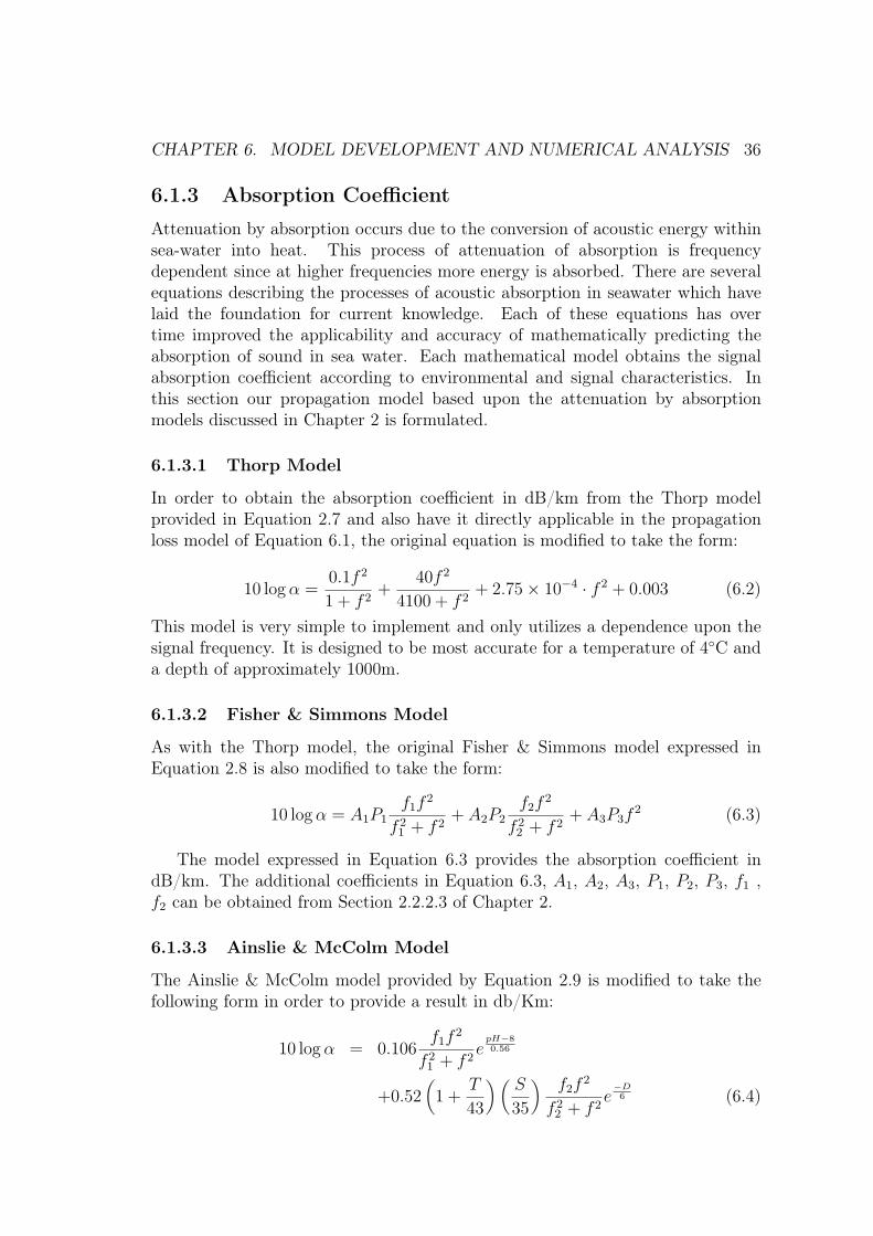
6.1.3 Absorption CoefficientAttenuation by absorption occurs due to the conversion of acoustic energy withinsea-water into heat. This process of attenuation of absorption is frequencydependent since at higher frequencies more energy is absorbed. There are severalequations describing the processes of acoustic absorption in seawater which havelaid the foundation for current knowledge. Each of these equations has overtime improved the applicability and accuracy of mathematically predicting theabsorption of sound in sea water. Each mathematical model obtains the signalabsorption coefficient according to environmental and signal characteristics. Inthis section our propagation model based upon the attenuation by absorptionmodels discussed in Chapter 2 is formulated.

6.1.3.1 Thorp Model

In order to obtain the absorption coefficient in dB/km from the Thorp modelprovided in Equation 2.7 and also have it directly applicable in the propagationloss model of Equation 6.1, the original equation is modified to take the form:

10 log α =0.1f 2

1 + f 2+

40f 2

4100 + f 2+ 2.75× 10−4 · f 2 + 0.003 (6.2)

This model is very simple to implement and only utilizes a dependence upon thesignal frequency. It is designed to be most accurate for a temperature of 4◦C anda depth of approximately 1000m.

6.1.3.2 Fisher & Simmons Model

As with the Thorp model, the original Fisher & Simmons model expressed inEquation 2.8 is also modified to take the form:

10 log α = A1P1f1f 2

f 21 + f 2

+ A2P2f2f 2

f 22 + f 2

+ A3P3f2 (6.3)

The model expressed in Equation 6.3 provides the absorption coefficient indB/km. The additional coefficients in Equation 6.3, A1, A2, A3, P1, P2, P3, f1 ,f2 can be obtained from Section 2.2.2.3 of Chapter 2.

6.1.3.3 Ainslie & McColm Model

The Ainslie & McColm model provided by Equation 2.9 is modified to take thefollowing form in order to provide a result in db/Km:

10 log α = 0.106f1f 2

f 21 + f 2

epH−80.56

+0.52(1 +

T

43

) (S

35

)f2f 2

f 22 + f 2

e−D6 (6.4)


+4.9× 10−4f 2e−( T27+ D

17)

The coefficients for the above equation may be obtained from Section 2.2.2.4of Chapter 2.

6.1.4 Ambient Noise ModelAmbient noise in the ocean can be described as Gaussian and having a continuouspower spectral density (p.s.d.). The four most prominent sources for ambient noiseare the turbulence, shipping, wind driven waves and thermal noise. The p.s.d. indB re µPa per Hz for each of these is given by the formulae [49] shown below:

10 log Nt(f) = 17− 30 log f (6.5)

10 log Ns(f) = 40 + 20(s− 0.5) + 26 log f − 60 log(f + 0.03) (6.6)

10 log Nw(f) = 50 + 7.5w12 + 20 log f − 40 log(f + 0.4) (6.7)

10 log Nth(f) = −15 + 20 log f (6.8)

The ambient noise in the ocean is colored and hence different factors havepronounced effects in specific frequency ranges. In the noise model equationsutilized for this study the colored effect of noise is represented by Nt as theturbulence noise, Ns as the shipping noise (with s as the shipping factor which liesbetween 0 and 1), Nw as the wind driven wave noise ( with w as the wind speedin m/s) and Nth as the thermal noise.

Turbulence noise influences only the very low frequency region, f < 10 Hz.Noise caused by distant shipping is dominant in the frequency region 10 Hz -100Hz. Surface motion, caused by wind-driven waves is the major factor contributingto the noise in the frequency region 100 Hz - 100 kHz (which is the operatingregion used by the majority of acoustic systems). Finally, thermal noise becomesdominant for f > 100 kHz.

The overall noise p.s.d. may be obtained in µPa from:

N(f) = Nt(f) + Ns(f) + Nw(f) + Nth(f) (6.9)

The noise p.s.d. may be used along with the signal attenuation to arrive at valuesthat characterize the channel performance. The obtained value may be convertedto dB by following the method described in Section B.2 of Appendix B.

6.2 The Underwater Acoustic Channel ModelSince the underwater acoustic channel is locally time varying, there exists no singlecharacter for the channel that could be globally used as a model. This makesit important to characterize the underwater acoustic communication channel inorder to determine the effects of local environmental phenomenon on achievable


performance. This performance of the channel can be characterized by propertiesthat include received signal power (which is dependent on the transmission power),signal-to-noise ratio (SNR) and the capacity bound.

6.2.1 Received Signal PowerThe path loss represented by Equation 6.1 is the attenuation that occurs on asingle unobstructed propagation path. As such, if a signal with frequency f istransmitted over distance l with a power Ptx then we can calculate the arrivingsignal power Prx in dB as:

10 log Prx = 10 log Ptx − 10 log A(l, f) (6.10)

The result obtained from Equation 6.10 takes into account only the case for adirectional transmission, i.e., the most direct propagation path from transmitterto receiver. However, in case of a transmission that is not directional needs tobe modelled, this equation can be extended for the indirect routes as well. Atpresent, in this work the focus is only upon the directional transmission model inorder to obtain the received signal’s p.s.d.

Since the received signal power is dependent upon the propagation loss factor,the attenuation model choice also adds a dependence upon depth, temperature,salinity and acidity of the specific oceanic region that is of interest.

6.2.2 Signal-to-noise ratioUsing knowledge of the signal attenuation A(l, f) and the noise p.s.d. N(f) theSNR observed at the receiver may be calculated. Extending Equation 6.10 we canarrive at the following relationship for obtaining the SNR in dB:

10 log SNR(l, f) = 10 log Ptx − 10 log A(l, f)− 10 log N(f) (6.11)

where SNR(l, f) is the SNR over a distance l and transmission center frequencyf . Similar to the received signal power, the attenuation model choice also adds adependence upon depth, temperature, salinity and acidity of the specific oceanicregion that is of interest, for the SNR.

6.2.3 Optimal Transmission FrequenciesThe attenuation noise (AN) factor, given by −[10 log A(l, f) + 10 log N(f)] fromEquation 6.11, provides the frequency dependent part of the SNR. By close analysisof this relationship, it can also be determined that for each transmission distancel there exists an optimal frequency at which the maximal narrow-band SNR isobtained. Since the SNR is inversely proportional to the AN factor, the optimalfrequency is that for which the value of 1/AN ( represented in dB re µPa per Hz) isthe highest over the combination of a certain distance, fo(l). Using these optimal


frequencies one may choose a transmission bandwidth around fo(l) and adjust thetransmission power to meet requirements of a desired SNR level.

All the formulation in this analysis work is based upon the optimal frequenciesfo(l), however, it may be extended to any desired frequency by replacing fo(l)with the chosen transmission frequency ftx(l) for a particular application.

6.2.4 BandwidthAuthors of [8] present capacity as a 3 dB band heuristic definition in their work,and we utilize the same definition for calculating the channel capacity. As such, theavailable bandwidth is a range of frequencies around fo(l), such that the differenceof A(l, fo(l))N(fo(l)) and A(l, f)N(f) is within the bandwidth definition. Here wecan define fmin(l) as the smallest frequency for which ANfo(l) − ANf ≤ 3 holdstrue and fmax(l) as the largest frequency f for which ANfo(l) − ANf ≤ 3 holdstrue as well. Thus, the transmission bandwidth B(l), over a distance l, becomes:

B(l) = fmax(l)− fmin(l) (6.12)

6.2.5 Channel CapacityUsable channel capacity is undoubtedly one of the best metrics since it governsmany aspects of network design and can lead to significant changes in topologies,protocols and access schemes utilized in order to maximize the overall throughput.As per the Shannon theorem the channel capacity C, i.e. the theoretical upperbound on data that can be sent with a signal power of S subject to additive whiteGaussian noise is:

C = B log2

(1 +

S

N

)(6.13)

where B is the channel bandwidth in Hz and SN represent the SNR. The basic

Shannon relationship shown in Equation 6.13 can be extended to be applicable incases where the noise is dependent on frequency to take the form of:

C =∫

Blog2

(

1 +S(f)

N(f)

)

df (6.14)

If we assume a time-invariant channel for a certain interval of time alongwith Gaussian noise then we can obtain the total capacity by dividing thetotal bandwidth into multiple narrow sub-bands and summing their individualcapacities. In this case each sub-band has a width of a small ∆f which is centeredaround the transmission frequency and this can be obtained from the relationshipdefined in Equation 6.12.

Extrapolating from the above discussed Equations 6.12 and 6.14, we may nowobtain the channel capacity over distance l from:

C(l) =∫

Blog2

(

1 +Ptx

A(l, f)N(f)B(l)

)

df (6.15)


6.3 Numerical EvaluationA deeper understanding of the propagation and channel models provided in theprevious sections of this chapter is important in order to optimally choose themodels for simulating underwater networks that utilize the acoustic channel.In this section we numerically evaluate the equations that are proposed in theprevious sections and also compare the results obtained by using different modelsto arrive at various conclusions.

0 10 20 30 40 50 60 70 80 90 1000

5

10

15

20

25

30

35

40

45

Distance (km)

Op

tim

al

Fre

qu

en

cy

(k

Hz)

ThorpAinslie & McColmFisher & Simmons

Figure 6.1: Optimal frequencies as predicted by the different channel models.

For the purpose of evaluation work, optimal frequencies for all transmissiondistances are utilized. Depth of 1 km, temperature of 4 ◦C, pH level of 8 andsalinity of 35 ppt are utilized for all numerical evaluations, unless otherwise stated,in order to remain within the capability ranges of all the attenuation models.

6.3.1 Optimal FrequenciesThe optimal transmission frequency provides the highest capacity and therebymost likely the best performance in the underwater acoustic channel. Acomparison of the optimal frequencies predicted by each of the three propagationmodels is shown in Figure 6.1. An analysis of this plot reveals that the Fisher &Simmons model provides optimal frequencies which are higher than those predictedby the Ainslie & McColm and Thorp models. The results of the Ainslie &


McColm and Thorp models are very similar, however, it is already known fromresults obtained in Chapter 2 that the Thorp model does not provide resultsthat are nearly as detailed as those provided by the Fisher & Simmons andAinslie & McColm models since the Thorp model only takes into account theeffects of transmission frequency on the attenuation coefficient, thereby limitingthe predicted channel characteristics to effects of distance and frequency only.

500 1000 1500 2000 2500 3000 3500 400021

22

23

24

25

26

27

28

Depth (m)

Op

tim

al

Fre

qu

en

cy

(k

Hz)

Fisher & Simmons

Ainslie & McColm

Figure 6.2: Optmial frequencies with changing depth.

The slight difference in the values between Ainslie & McColm and Thorpmodels can be attributed to the lack of channel characteristics parameters inthe Thorp model. However, since we are mostly interested in the deep seaacoustic channel, it is important to take into account parameters such as depth,temperature, acidity and salinity in order to obtain an accurate representation ofthe underwater acoustic channel. This requirement makes the Ainslie & McColmand Fisher & Simmons models of greater interest to us. A comparison of theresults provided by both these models shows a relatively large difference in theoptimum frequency predicted. This can mostly be attributed to the fact that theAinslie & McColm model is a simplified model, which obviously introduces someerrors.

However, since the results provided by the Ainslie & McColm model arebetween those provided by the other two models, both of which are widelyutilized in published literature, it appears to provide a good approximation ofoptimal frequencies (and thereby other channel results) as well. The additional


computational overhead added by the multiple parameters, however, makes it moreappealing to utilize the Thorp model when approximations are needed.

Using this conclusion as a basis, a comparison of the optimal frequencies aspredicted by the Ainslie & McColm and Fisher & Simmons models with varyingdepth is provided in Figure 6.2. A transmission range of 500 m is used to obtainthese results. It is clear from this plot that optimal frequencies increase with theincrease in depth. Both models show this increasing trend, however, once againthe Ainslie & McColm model predicts values lower than Fisher & Simmons fordepths below 3500 m.

0 5 10 15 20 25 30 3522

23

24

25

26

27

28

29

30

31

Temperature (°C)

Op

tim

al

Fre

qu

en

cy

(k

Hz)

Ainslie & McColm

Fisher & Simmons

Figure 6.3: Optmial frequencies with changing ocean temperature.

Being interested in deep sea acoustic channels it is important to keep in contextof analysis the halocline and thermocline as well. A detailed discussion of these twocharacteristics is provided in the Appendix, however, it is necessary to highlightthat the ocean temperature varies between -2◦C and 36◦C while the salinity onlyvaries between 33-37 ppt with depth. The global oceanic acidity remains quiteconstant around a pH value of 8, besides specific regions such as underwatervolcanoes. Keeping these values in mind a plot of optimal frequencies with varyingtemperature is provided in Figure 6.3. A transmission distance of 500 m is utilizedto obtain results for this graph.

At first glance the results in Figure 6.3 make it appear as though the Ainslie& McColm model has an anomalous performance as compared to that of theFisher & Simmons model since basic logic dictates that optimal frequency should


increase with temperature as almost a linear relationship, much like that withdepth. However, further analysis reveals that at 1 km depth the density of wateris actually highest at 4◦C, thereby representing a curve that looks almost paraboliccurve [50]. Comparing this behavior of water density with the plot in Figure 6.3reveals that the Ainslie & McColm provides results which adhere to this ideology.This result makes it clear without any doubt that the Ainslie & McColm modeloutperforms Fisher & Simmons, thereby making it the model of choice.

33 33.5 34 34.5 35 35.5 36 36.5 3729.1

29.2

29.3

29.4

29.5

29.6

29.7

29.8

29.9

30

30.1

Salinity (ppt)

Op

tim

al F

req

uen

cy (

kH

z)

Figure 6.4: Optmial frequencies with changing ocean salinity.

The plot in Figure 6.4 clearly shows that the optimal transmission frequencyreduces with changing salinity, however, the overall change of 1 kHz over the rangeof possible ocean salinities is quite neglegible and therefore does not pose a greateffect on the performance of the underwater acoustic channel.

6.3.2 Bandwidth and CapacityOptimal transmission frequencies were evaluated at various depths, temperaturesand transmission distances in order to derive the patterns of effects that theseparameters would have on the predicted channel capacity. For the purpose ofevaluating ambient noise we assumed a shipping factor s = 0.5, to representmoderate shipping, and no wind-caused waves leading to a w = 0. Since wewere able to determine in the previous section that the Ainslie & McColm modelprovides results that are more accurate than the Fisher & Simmons model, theBandwidth and Capacity investigations were done using the Ainslie & McColm


model. Furthermore, a comparison with the Thorp model was undertaken toprovide a comparison between the models.

Figure 6.5: Effect of depth on available bandwidth.

In Figure 6.5 we plot the effects that depth and signal transmission distancehave on bandwidth. The plot indicates that available bandwidth increases almostlinearly with increasing depth, however, this linear effect is not constant over everytransmission distance; the shorter the transmission distance, the more quicklybandwidth increases with depth. This clearly indicates that having networkdesigns with short transmission distances would make better use of channelcapacity and thereby provide an overall higher throughput. Depending upon thedepth of the transmitting nodes the channel bandwidth can vary even as high as11 kHz for a particular distance; on an average the bandwidth varies by 5 kHz asan effect of depth and transmission distance.

Since the Ainslie & McColm model also allows us to evaluate effects oftemperature on bandwith and capacity we evaluated the variance of bandwidthwith temperature and multiple transmission distances. Figure 6.6 shows a plotthat displays the effects of temperature on bandwidth when multiple signaltransmission distances are used. For the purpose of this evaluation a fixed depthof 500 m and temperatures ranging between -2◦C and 36◦C were used.


Figure 6.6: Effect of changing temperature on bandwidth.

From the plot in Figure 6.6 it becomes quite clear that increasing temperaturegenerally causes bandwidth to increase, however, this relationship is not linear.Furthermore, at comparatively shallow depths (at least till 1 km depth) thebandwidth decreases from -2◦C till a certain point before increasing again. Suchnon-constant increase or decrease in capacity makes it critical for underwateracoustic systems, at least mobile ones, to be designed with this in mind. Since theshallow water region normally comprises of the thermocline where temperaturefluctuations can occur over the course of the day, shallow water networks wouldgreatly suffer in performance unless they stick to the minimum bandwidth or followadaptive bandwidth schemes.

The effects of temperature and depth on channel capacity are also investigatedin order to have a more concrete picture. The channel capacity calculated usingEquation 6.15 is plotted in Figure 6.7 for a comparison on the effects of depth andtemperature. The plot presents the effects of temperature on capacity while alsovarying the depth but keeping the transmission distance fixed at 5 km. Just aswith bandwidth, channel capacity increases with increasing depth and temperaturealso appears to have the same effect. In case of deep sea nodes or even mobilenodes, the network and protocols could be designed to take benefit of this fact byallowing deeper nodes to communicate at higher bandwidths to achieve an overallhigher throughput.


6.3.3 Discussion

Figure 6.7: Effect of changing temperature on capacity.

An initial comparitive numerical analysis of the three different underwater acousticpropagation and channel models reveals that even though the Fisher & Simmonsmodel is one of the most popularly utilized models in published literature, theresults it provides are not as accurate to those provided by the Ainslie & McColmmodel. Furthermore, the ability to simulate effects of depth, temperature, salinityand acidity also make the Ainslie & McColm model comparatively highly desired.The Thorp model provides a good approximation of performance since it’s resultsare closest to that of the Ainslie & McColm model at it’s default channelcharacterisitc parameters. Since changing the model used changes the resultssignificantly it is important to make an appropriate choice.

Furthermore, it is quite clear after the numerical evaluations that acidity doesnot have a pronounced effect on the channel performance characteristics, however,salinity, temperature and depth all have an effect that make it important to samplethese values when designing a network topology or choosing acoustic modems fora particular application. It can also be said with high confidence that bandwidthand capacity decrease over longer transmission distances, while increasing depthprovides higher bandwidths and capacity; the relationship between temperatureand capacity and bandwidth is not linear but can be generalized to be mostlyincreasing with increasing temperatures.


The optimal transmission frequencies for longer transmission distances arelower but increasing the depth and termperature mostly increases the optimaltransmission frequencies. The only anomaly in this relationship is due to thedensity of water being effected by temperature, thereby making the relationshipbetween temperature, water density and optimal frequency a non-linear one.

Chapter 7

Software Implementation

Numerical analysis provides results which are interesting and can lead towardsinitial network design choices that could enhance overall network performance.However, network performance is not only dependent upon the physicalcharacteristics of the underwater acoustic channel. In order to provide an overallperformance analysis it is important to also evaluate the network statistics whichresult from media access control schemes, routing protocols, modulation schemesand other networking layers. In order to do so, it is important to build asoftware infrastructure that takes into account a complete acoustic propagationand channel model and implements them such that it can provide details onachievable (or achieved) data rates, performance of routing protocols, deliveryratio of packets and other characteristics. Furthermore, even though numericalmodels can represent propagation and physical layer issues, they fail to incorporateprotocol issues such as collisions and multiple-access interference.

The NS-2 simulator, which is a highly popular tool used for simulating networkperformance, provides an excellent basis to develop a software implementationfor simulating the underwater acoustic channel. This chapter disucusses theimplementation of the AquaTools NS-2 underwater simulation toolkit whichincorporates various channel models constructed in Chapter 6 into NS-2 in order toensure that all conditions effecting the performance of a network can be analyzed.The trace files provided by NS-2 could be further useful in research to tweak andmaximize network performance. It also covers the Wireless Simulation Server thatwas designed for the USARSim high-fidelity real-time robotics simulator in order toprovide a platform to quickly test and evaluate the performance of an underwateracoustic network on mobile robot nodes, while keeping in mind the requirementfor active environmental sensing and movement responses that a robot would haveand which NS-2 cannot account for.

48

CHAPTER 7. SOFTWARE IMPLEMENTATION 49

7.1 The AquaTools NS-2 Underwater SimulationToolkit

The NS-2 simulator divides the channel and physical layer functions andcharacteristics into four components, namely Propagation, Channel, Physical,and Modulation. Figure 7.1 depicts this division, highlighting the characteristicswithin each component. The propagation component contains most ofthe characteristics of the signal propagation through the medium (includingattenuation) and of the ambient noise. In addition to distance-dependentattenuation, in underwater channels the signal fading is also affected by theorientation of the link. This feature is also modeled in the propagation component.The characteristics exported to other components of the NS-2 model include thecalculation of the received signal strength and the interference range of a signal.

Interference Range

Received Signal Strength

Bandwidth

Propagation Delay

Interfering Node Set Number of

Bit Errors

Channel

Model

Physical

Model

Propagation

Model

Modulation

Model

Packet Error

Time of Packet Reception

Energy Computation

Remaining Battery

Figure 1: The ns2 channel and physical layer model

thorp(frequency)1 f ← pow(frequency,2);2 if f > 0.43 then4 atten← 0.11 ∗ f/(1 + f)+5 44 ∗ (f/(4100 + frequency))+6 2.75 ∗ pow(10,−4) ∗ f+7 0.003;8 else9 atten← 0.002+

10 0.11 ∗ (f/(1 + f))+11 0.011 ∗ f ;12 return atten;

Figure 2: Thorp’s approximation

divides the frequencies into two groups, those under 400 Hz(see Figure 2, lines 2–7), and those over 400 Hz (see Figure 2,lines 8–11). We chose to use dB re µPa throughout ourimplementation, as this is a typical unit of signal strengthin acoustic communications. Accordingly, all quantities aregiven using these units, and all tunable parameters (in termsof transmit power for example) should be given in dB re µPaas well.

Combining absorption effects and spreading loss, the totalattenuation is as follows [22]:

10 log A(!, f) = k · 10 log ! + ! · 10 log a(f), (2)

where the first term is the spreading loss and the second termis the absorption loss. The spreading coefficient defines thegeometry of the propagation (i.e., k = 1 is cylindrical, k = 2is spherical, and k = 1.5 is practical spreading [22]). Thisis used in the calculation of the SNR at the receiver (in afunction that overloads the Pr function in ns2)in combina-tion with the ambient noise calculation (see Figure 3 lines5–6).

Pr(transmitter, receiver)1 Pt← transmitter→ getTxPr();2 distance← calcDist(transmitter, receiver);3 for i← 0 to NUM FREQ4 do5 AN [i] ← −(k ∗ 10 ∗ log10(distance)+6 distance ∗ thorp(freq[i])+7 orientation(transmitter, receiver)+8 log10(noise(freq[i])));9 if AN [i] > AN [max index]

10 then11 max index← i;12 Pr ← Pt + AN [max index];13 return Pr;

Figure 3: SNR at the receiver

In addition to this attenuation, signal fading in the under-water environment is affected by the orientation of the link(i.e., whether the link is horizontal or vertical). To accountfor this effect, we added a modifier function that takes thelocation of the sender and receiver and returns an additionalattenuation factor that is combined to account for the totalattenuation (Figure 3, line 7).

The calculation for the ambient noise in the underwaterenvironment (see Figure 4) is divided into the major factorscontributing to the total: turbulence (Figure 4, lines 1–2),shipping (Figure 4, lines 3–7), wind (Figure 4, lines 8–12),and thermal (Figure 4, lines 13–14). The following formulaegive the power spectral density of the four noise components

Figure 7.1: The NS-2 channel and physical layer functional model

The primary function of the channel model is to handle propagation delaycalculations and to make use of the functions from the propagation model.The physical layer tracks energy consumption metrics and also calculates thetransmission times. Unlike in radio models, where the bandwidth is assumedto be constant regardless of the transmitter-receiver distance, depth, ambienttemperature, salinity or acidity and therefore no information for other layersis required, in an underwater network the link bandwidth does depend on thelink length, and therefore bandwidth information from the propagation layer ofNS-2 must be exposed to other components. Finally, the physical model callsthe modulation model to calculate bit error probabilities given a received signalstrength, modulation scheme, and level of noise. It is interesting to note thatno standard modulation schemes are currently used in the majority of NS-2simulations.


The AquaTools toolkit uses dB re µPa as the unit of sound energy throughoutthe entire implementation since this a typical unit of signal strength which is usedin acoustic communications. Accordingly, all quantities expressed here are in thisunit, and all tunable parameters (for example, transmit power) are also given indB re µPa as well.

7.1.1 Underwater Propagation ModelIn NS-2, the Propagation models are responsible for calculating the signal-to-noiseratio at the receiver after attenuation and ambient noise are taken into account,as well as the interference range of a signal.

The AquaTools implementation only requires the user to choose theappropriate underwater propagation model in the TCL simulation script usingthe names for the respective propagation model based on the namesake of thepath loss model that forms its basis:

Propagation/UnderwaterThorp

Propagation/UnderwaterFisherSimmons

Propagation/UnderwaterAinslieMcColm

To calculate the signal-to-noise ratio (SNR) at the receiver and the interferencerange, both the attenuation of the acoustic signal in water and the ambientnoise need to be accounted for. The total attenuation is calculated based on thespreading loss, ambient noise and the signal attenuation. The signal attenuationis obtained from either of the Equations 6.2, 6.3 or 6.4 depending upon the pathloss model that is chosen as the basis of the underwater propagation model.

The ambient noise in the underwater environment is contributed majorly byfour factors; namely, turbulence, shipping, wind and thermal. The effect of eachof these components of ambient noise in the underwater environment may beobtained from Equations 6.5, 6.6, 6.7 and 6.8 which were discussed in Section6.1.4. A total effect of the noise model may be arrived at by using Equation 6.9and then converting the obtained value to dB re µPa by using the relationshipsexpressed in Equations B.1 and B.3.

By default the values for the shipping variable, s, and the wind variable,w, are set to 0. These variables are bound to TCL variables called ship_ andwind_ respectively and can be set in the usual way with lines such as:

Propagation/UnderwaterThorp set ship_ value

Propagation/UnderwaterThorp set wind_ value


where ship_ can take values from 0 to 1 and wind_ , which represents wind speed,can take positive values in m/s.

Combining the effects of path loss due to absorption and taking into accountthe spreading loss as well, the total signal attenuation at the receiver is calculatedusing Equation 6.1. The value obtained here is used in the calculation of the SNRat the receiver in combination with the ambient noise calculation. This calculationis done by a function that overloads the Pr function of NS-2 and uses a form ofEquation 6.10 to arrive at a result of the received power.

The NS-2 simulator has a node class that keeps information specific to eachnode in the simulation, including location coordinates (x, y, z) and transmitpower settings. The node class also has a number of member functions usedto access information about the nodes. The Pr function takes pointers to thetwo communicating nodes and is used by the Channel model in the calculation ofpacket loss probability. To find the attenuation for a given transmission betweentwo nodes, the center frequency for the transmission must be found. In theimplemented model, this corresponds to the frequency that exhibits the bestpropagation conditions, for a specific distance between the communicating nodes.

As such, in order to obtain this center frequency, the SNR may be expressedas in Equation 6.11 or as a simple function of frequency, which is given by:

SNR(l, f) =Ptx

A(l, f)N(f)(7.1)

This representation makes it clear that the SNR is inversely proportional to theAN factor. As already discussed in Section 6.2.3, the optimal frequencies are thosefor which the 1/AN value is highest. Keeping this in mind, in order to obtain thecenter frequency, and thereby the received signal strength, the distance betweennodes is calculated. The AN factor for every possible transmission frequency isthen calculated and the frequency with the lowest AN factor (largest value of theAN variable) is tracked. Finally, the AN factor that corresponds to that frequencyis combined with the transmitted power to calculate the SNR at the receiver andis taken to be equal across the the frequency spectrum.

The NS-2 propagation model is also expected to define the radius inwhich a transmission needs to be considered for interference with other nodes’transmissions. The function getDist takes a threshold received power level, thetransmit power level and the frequency at which the signal was sent, and returnsthe largest distance that a node should be from the transmitter and still beconsidered interfered with by its transmission.

Essentially, this function finds the target attenuation that is needed to resultin a received signal strength so low that it does not need to be considered forinterference calculations. It then iteratively calculates the attenuation at distancesstarting at one meter until it finds the target factor. This function is only accurateto the closest meter.

The results obtained by the propagation model are by the channel modelto make collision and transmission error decisions. As such, it does not need


to calculate propagation delay or bandwidth. However, these functions areimplemented in the channel model, which is described in detail further.

7.1.2 Underwater Channel ModelThe channel model in NS-2 maintains the node lists used to calculate neighborsets, collisions and etc. It is additionally responsible for calculating propagationdelays. Essentially, the physical layer calls a sendUp function with a packet and apointer to itself, and the channel model calculates neighbors that may be affectedby the transmission as well as propagation delays and returns this information.Full details on the exact functionality of the NS-2 simulator can be found in theNS-2 manual [51].

Aside from calling the appropriate propagation model functions, such asgetDist, the NS-2 channel model has to implement the propagation delay modelas well, which is somewhat complex due to the dependency of the speed of soundon the depth of the water. In addition to the depth in the water, the propagationspeed also depends on the temperature and salinity of the water, which in turndepend on the depth through a non-linear relationship. A sample of this non-linearrelationship can be seen in Figures A.1 and A.2 of Appendix A.

Figure 7.2: Implementation of the getTemperature and getSalinity functions whichprovide respective values as a function of depth according to the globally observedaverage thermocline and halocline.

In order to provide a realistic simulation, the global average observedthermocline and halocline are modelled within the AquaTools implementation asthe functions getTemperature and getSalinity, which provide the temperatureand salinity, respectively, as a value which is proportional to the current depth.

With these values obtained the speed of sound can be modelled easily usingthe relationship defined in Equation 2.1. There are only five known ocean zoneswhere the speed of sound can be expressed as a linear relationship [7], and only


for these zones the simulator would not provide results which should be closelymatched to reality.

In order to calculate the propagation delay, the getPDelay function takessegments of distance traveled depending on the nodes’ depth and calculatesdistance traveled divided by the speed. When all of the segments of the pathhave been added together, the total propagation delay is returned. A functionSetDistV ar takes the current values of the highest and lowest depth (z-variables)and returns the distance traveled in the next segment of linear temperature change,the average temperature in that zone and the updated values for the z-variables.

To use the underwater channel model, it is only necessary to choose it in theTCL simulation script using the name, Channel/UnderwaterChannel.

There is only one bound variable in the channel model that may be set by theuser in order to override the getSalinity function. The salinity value for the waterused in the propagation delay calculation can be set to some other value than theone returned by getSalinity as shown below:

Channel/UnderwaterChannel set salinity_ value

The physical layer model uses information from both the channel model and thepropagation model to calculate transmission times, total delays, and the success orfailure of packet reception. The physical layer model is described in detail further.

7.1.3 Underwater Physical Layer ModelThe physical layer model of NS-2 calculates the final statistics used in thesimulation with respect to packet reception, including packet error, transmissiontime, and propagation delay. For most of these calculations, calls are made tofunctions in the channel and propagation models. Additionally, information aboutenergy costs associated with the physical interface are stored and used to calculateresidual battery charge and transmission energy costs.

All the specific parameters of interface energy consumption are implemented asbound variables to be set by the user, since they depend on the specific hardwarebeing modeled. Additionally, the received signal strength threshold and themaximum transmit power levels are interface specific and are set through boundvariables. The default sets of parameters for the maximum transmit power, receivethreshold, and the interface energy consumption parameters are set to model theWHOI micromodem [52], since this appears to be a modem that is used most oftenin academic research due to it’s open design and platform. All these parameterscan be set up using the normal TCL statements which are used to set up theinterface parameters of wireless radio devices in the 802.11 physical layer modelas well.

To use the underwater physical model, it is only necessary to choose it in theTCL simulation script using the name:

Phy/UnderwaterPhy


To set the maximum transmit power and the receive threshold, set the variablesPt_ and Pr_ respectively (units in dB re µPa) as shown below:

Phy/UnderwaterPhy set Pt_ value

Phy/UnderwaterPhy set Pr_ value

The primary function of interest used in the physical layer is the calculationof the available bandwidth given the distance between the transmitter andreceiver, their depths and the ambient environmental conditions. Even thoughthe bandwidth calculation function getBandwidth() resides in the propagationmodel it is described here since this is the only place where it is used. First, usingthe distance between the transmitter and receiver, the frequency experiencing theminimum AN factor is found (optimum frequency). This frequency is used asthe center frequency for communication. Then, the 3 dB definition of bandwidthis used to find the edges of the usable frequency band and then bandwidth iscalculated as per Equation 6.12 and returned.

7.1.4 Underwater Modulation ModelThe Modulation model in NS-2 is responsible for bitrate and bit error calculationsbased on signal strength and modulation scheme utilized. The error probabilityis a function of the SNR. The bitrate and number of bit errors is returned by themodulation model.

Even though many modulation schemes have been briefly discussed in Chapter3, none have been specifically implemented within the AquaTools simulationtoolkit since this was presently beyond the scope of this work as it is evidentfrom current literature that not enough investigation work has been done to devisemathematical models that quantify the performance of a particular modulationscheme. As such, the only results available, which are few, are based completelyupon experimental observations in off-shore testing and are not numerable enoughto formulate mathematical models that could be implemented in the simulator toobtain dependable results. The development of mathematical models that coulddependably predict the performance of modulation schemes remains a topic forfuture research.

As a result, the AquaTools simulation toolkit currently utilizes the wirelessmodulation scheme as it is provided with an NS-2 distribution in order toperform the bit error calculations. The bitrate utilized is limited to the capacitypredicted by an implementation of the Shannon capacity theorem, a mathematicalrelationship for obtaining which was provided in Equation 6.15.

The modular nature of NS-2 ensures that, when a competent mathematicalmodel for effects of modulation schemes on bit-rates and bit-error rates isdeveloped, it could be easily implemented and replace the current one.


7.2 The USARSim Wireless Simulation ServerUSARSim is a high-fidelity simulation tool for simluation robots and environmentsbased on the Unreal Tournament game engine. The software is specificallydesigned as a research tool and is the basis for important current-day roboticsimulations, the most famous being represented by the RoboCup rescue virtualrobot competition. The advantages of USARSim consist of the ability to offloadthe most diffcult aspects of simulation to a high volume commercial platform,which provides superior visual rendering and physical modeling. Therefore, theentire effort can be devoted to the robotics-specific tasks of modeling platforms,control systems, sensors, interface tools and environments. Further advantagesthat confirm USARSim as a leading robot simulation environment include thepresence of development tools integrated with the game engine and advancedediting features for almost every aspect of the simulation, with a special focuson robots and environments. All this functionality allows for a wide range ofrobot tasks and simulations that can be modeled with greater fidelity in less time.USARSim can also be used to simulate scenarios involving cooperative operationof multiple robots.

All these advantages and its modular nature in developing new additions forsensors, modules and ability to model complex underwater environments makesit a suitable tool to model the multi-AUV underwater acoustic communicationsas well. This section discusses the underwater environmental and submersiblevehicle modelling capabilities of USARSim along with information on the WirelessSimulation Server and the extensions made to these tools in order to enable mobilemulti-AUV communication simulations.

Although a part of this work, involving the development of the basic simulationtool was done for a Robotics seminar, the rest of the work of extending theenvironment to support models besides Thorp and Fisher & Simmons, calculationof bandwidth (not capacity) and the optimal frequency were performed during thecourse of this investigation in order to leverage the real-time capabilities of thisenvironment.

7.2.1 Underwater Vehicle and Environment ModelIn order to correctly evaluate the communication model and test the effects ofalgorithms, methods and control schemes, it is important to have environmentand robot models that mimic reality. USARSim has a model world that simulatesan underwater environment available by default, but others can also be easilycreated using the Unreal Tournament model editor. The default model, shown inFigure 7.3 is used for all the testing associated with the development work.

Along with the underwater world model it is also necessary to have an accuratemodel of the vehicle to be simulated. This ensure physically accurate simulationsof the responses and behavior of a vehicle which in turn assists in accurately testingthe performance of an underwater acoustic network. Though any vehicle models


can be created and imported into the USARSim environment, a Submarine model,which is deisgned keeping in mind all physical properties, is provided by default.This model can have sonar sensors, imaging sensors, echo sounders, side scan andan optical camera simulated on it.

Figure 7.3: Screenshot of the USARSim default model and submarine

All the data, including robots, sensors and other devices, associated withUSARSim within Unreal Tournament are accessed and manipulated by usingTCP/IP socket connections. In order to simplify the interfacing of testscripts and/or software, an interface library developed by the Jacobs UniversityRobotics Group was utilized to spawn connections with the USARSim SimulationEnvironment.

The default implementation of the interface library for USARSim did nothave an implementation of a driving mechanism for the submarine and as such adrive mechanism for the propeller, rudder and stern planes was implemented,thereby providing full mobility control of the submarine and giving access totesting mobile-AUV communications by taking into account real-time decisionsand responses made by submersible vehicles.

7.2.2 Wireless Simulation ServerAn USARSim plugin called the Wireless Simulation Server (WSS) enablessimulation of 802.11 wireless network links within the USARSim environment.WSS works using plugins to implement propagation models allowing forextensibility in the future. The degradation of the arriving signal at the receiving


vehicular node is calculated based upon parameters that are setup for thepropagation model plugin and which governs whether connection between robots ispossible or not. WSS maintains a table of all USARSim nodes and also informationon whether a connection between them, dependent on the propagation modelutilized, is possible or not.

Figure 7.4: Screenshot of the USARSim WSS capable of simulating underwaternetworks

A connection model similar to that of USARSim is utilized by WSS tocommunicate with all the robot nodes spawned within USARSim. A TCP/IPsocket connection is opened by each robot node within the USARSim simulator toWSS in order to query for available nodes, evaluate channel characteristics, checkthe possibility of connection to another robot and also send data to the remoterobot node.

Using this model as a basis the propagation and channel models discussed inChapter 6 and previous sections were implemented as propagation model pluginsfor WSS. The model configuration dialog shown in Figure 7.5 shows how themodels were designed with flexibility in mind so that the user could configure theambient noise parameters to suit the real environment being modeled. The modelconfiguration dialog also allows the user to easily configure the signal transmissionstrength, signal cutoff strength, bandwidth and center frequency in order to easilymodel any modem available without making changes to WSS or USARSim.


Figure 7.5: Screenshot of the propagation model configuration window

Since USARSim does not have a way to provide the depth of the robot toWSS, a sea level function which defines the sea level in the world map being usedwas implemented so that the robot’s depth could be calculated using its cartesiancoordinates, which are available to WSS by directly querying the USARSim server.This depth is utilized in order to determine the temperature and salinity at thecurrent depth from an implementation of the global thermocline and haloclineaverages in order to compute the propagation delay and attenuation coefficient.

In it’s native form, WSS only supports the functions of robots being able toretrieve signal strength from WSS for the target robot and determine whetherconnection is possible based upon this information and the modem properties.The following commands can be issued over the TCP/IP socket connection inorder to retrieve the signal strength information:

GETSS returns the signal strength at the target robot from the current positionof the querying robot.

The unit of the returned data is dB re µPa. However, this limitation is inadequatefor the underwater networking scenario where the ability to retrieve propagationdelay and channel capacity is also important. As such the following commandswere also implemented:

GETPD returns the propagation delay between the querying robot and thetarget robot specified in the query string.

GETBW returns the channel capacity in kbps between the querying robot andthe target robot specified in the query string.

These functions utilize the same strategy of calculating the propagation delayand bandwidth as was implemented within the different propagation and channelmodels for the NS-2 simulator.


A major advantage of the USARSim simulation environment over NS-2, besidesthe ability to account for realtime robot node reactions to the environment, is thatof being able to successfully emulate an underwater environment. In other words,the environmental modelling ability gives the capability of also modelling andobtaining a surface bottom profile of the ocean floor. This is extremely helpfulsince the surface bottom of the ocean is a great contributor to signal interferenceas a result of reflections that occur from the seabed in shallow water acousticcommunications. Furthermore, the surface bottom profile can have a significanteffect upon multi-path propagation interference as well. As such, it is importantto be able to test the likelihood of this factor interfering with the transmissionsignal. In order to implement the ability to test for surface bottom multi-pathsignal interference WSS was extended to support the following function as well:

GETML returns the interference likelihood as 0 or 1 for a distance to the surfacebottom provided in the query string.

In order to use the GETML function the submarine has to have a scanningsonar mounted. The scanning sonar obtains a bottom profile of distances to thesurface and these are supplied to WSS using the GETML function. An overallmulti-path likelihood using the surface bottom profile supplied by the scanningsonar is calculated by testing each individual acoustic channel pathway caused byreflections from the surface bottom for the arriving signal strength at the receivingrobot node. In case the receiving signal strength of any of the surface bottomreflected paths is equal or greater than the cutoff strength of the modem, aninterference likelihood of 1 is indicated. This may also be modified to representthe likelihood as a percentage value by calculating the number of total reflectionssuccessfully causing interference against those that do not.

7.3 DiscussionAs part of this thesis investigation work, the propagation and channel modelsthat were developed in Chapter 6 have been implemented within the frameworkof a toolkit for the NS-2 networking simulator. This toolkit, named AquaTools,provides access to Propagation, Channel and Physical layer models which aresuitable for the underwater acoustic channel, but does not provide a modulationmodel since currently there does not exist enough experimental information orbasic theoretical models from which a mathematical model suitable for this taskcould be extrapolated.

The implementation of an underwater acoustics channel model in NS-2 providesresearchers tools to be able to test multiple different protocols, strategies andmethods for tweaking or developing underwater acoustic communication systems.Furthermore, the familiar working environment of NS-2 is retained by AquaToolsin the form of setting up experiments easily and quickly via the TCL scriptinterface.


The developed propagation and channel models were also implemented withinthe framework of the USARSim mobile robotics simulator. In addition tosimulating the signal strength, propagation delay, connectivity achievability andchannel capacity, the WSS plugin implementation also provides the ability tosimulate and provide information on the surface bottom reflective interferenceas a result of the ability to simulate an underwater environment inherent withinUSARSim.

The WSS approach provides a significant upper hand over the NS-2implementation in the form of being able to provide information on surface bottomreflection interference likelihood. Furthermore, the ability to simulate events ina realtime fashion rather than depending upon pre-generated mobility scripts,as is the case with NS-2, can also be viewed as an advantage, especially forscenarios where the mobility pattern of the nodes being investigated cannot beprecomputed and may be dependent upon complex environmental interactions.However, this advantage posed by WSS is mitigated since there is no ability tosimulate the effects of protocols, modulation schemes and access control by usingthe WSS approach. On the other hand NS-2 provides the advantage of access tothese abilities and also being able to simulate complex network behavior such ascollisions and multiple-access interference.

Chapter 8

Simulator Validation

Both simulators developed as part of this work, the AquaTools NS-2 Toolkit andthe USARSim WSS plugin, provide generic tools to the underwater acousticscommunication community in order to test and develop underwater acousticcommunication systems. Having focus upon two of the largest different usergroups for such systems, one networking and the other robotics, these simulationenvironments provide not only tools that would be very valuable but also thosewhich are within frameworks familiar and often used within these communities.However, before any simulation tool can be utilized to take dependable designdecisions, it is required to validate the results obtained from the simulator inorder to ensure that they confom to those that are available within publishedliterature or they conform to those expected from numerical models utilized andpublished in literature.

The numerical evaluation of the propagation and channel models carried outin Chapter 6 already establishes the initial soundness of the models. Furthermore,since the models which form the basis of the overall propagation and channelmodels are widely used and published in academics, they can be viewed asdependable. In fact, similar design methodology followed in this work has alreadybeen utilized in other published work [8, 7, 53], thereby pointing towards thesoundness of the mathematical models used. The results achieved by the numericalanalysis are in line with those expected from published literature [8, 53].

Even though this points towards a sound mathematical model for thepropagation and channel models, mathematical verification only supports the casefor their utilization in the simulator. The results provided by the simulator alsoneed to be validated in order to ensure that these are within expected margins ofthe numerical models and closely mirror those already in literature.

Only upon successful validation can the simulators be used to set upexperiments which can be utilized to derive results that can aid in developmentof technologies supportive of underwater acoustic communications. To validatethe implemented underwater models in both the simulators, a number ofsimulations were run and the resulting values of specific parameters compared withthose calculated using analytic models and published literature, where available.

61

CHAPTER 8. SIMULATOR VALIDATION 62

Specifically, it was considered important to validate the major characteristics ofthe simulator; namely, noise, AN factor, optimal frequency, propagation delay,bandwidth and capacity to ensure there were no errors in the implementations.As will become evident from the presented results, the results obtained from boththe simulators matched the analytical model and also the published results whichwere available for comparison.

Both simulators are designed with the same basic propagation and channelmodels and consequently the results from one simulator can easily be obtained inthe other simulator as well. As such, for all the verification cases, the presentedresults are from one of the simulators, but tests were carried out in both simulatorsto ensure accuracy of results.

8.1 Noise

0 1000 2000 3000 4000 5000 6000 7000 8000 9000 1000020

22

24

26

28

30

32

34

Distance (m)

No

ise (

dB

re µ

Pa)

Fisher & Simmons

Ainslie & McColm

Thorp

Figure 8.1: The changing ambient noise as per changing distance which effects theoptimal frequency used for noise calculation.

The noise calculations are critical for calculating all the important parameters ofthe propagation and channel model, such as bandwidth, capacity and SNR. Assuch it was considered vital to evaluate the accuracy of the simulators in calculatingthe noise.

The noise predicted as per all the three models is plotted in Figure 8.1. Theoptimal frequency for transmission is used to arrive at an estimate of the ambientnoise since the optimal frequency provides the best case performance. The results


shown here are from the AquaTools NS-2 Toolkit, however, the results producedby the USARSim WSS environment were exactly the same. The minor differencesin the shape of the curves can be attributed towards the fact that each modelaccounts for different environmental parameters and as it is already known fromChapter 6 that the Ainslie & McColm model outperforms the other two modelswhich provide the upper and lower bound in this case.

Figure 8.2: The ambient noise as obtained by the simulative and analytical studyconducted by Harris et al. while using the Thorp model [7].

While the noise is not dependent on the transmission distance, verifying thisresult is necessary since ambient noise is dependent upon the frequency usedfor transmission and thereby, here it indicates whether the optimal frequencypredicted by the used models is accurate or not. When compared to the alreadypublished results of ambient noise within the work performed by Harris et al.[7], the results of which can be seen in Figure 8.2, we can easily notice that thecurves are very similar. In fact, upon close scrutiny, it is evident that the resultspredicted by the simulator while using the Thorp model are exactly the same asthose predicted in published literature [7].

While there is no direct comparison available to verify the results from theother two models, the results available are within expectations. This combinedwith the accuracy of the simulators while using the Thorp model argues in favorof the accuracy of the models and the simulation environments.


8.2 Propagation DelayTesting the accuracy of the propagation delay calculation requires a numberof experiments since the result depends on the depth of the communication inthe water. The test cases used in the simulator utilized two nodes, with onetransmitting data to the other. The depth of both the nodes were also varied whilesimultaneously changing the distances. The results that were obtained appearedto be within expected parameters since the shape of the propagation delay shouldclosely mirror that of the halocline and thermocline models being utilized [54].

0 500 1000 1500 2000 2500 3000 3500 4000 45000.65

0.655

0.66

0.665

0.67

0.675

0.68

Depth (m)

Pro

pag

ati

on

Dela

y (

s)

Figure 8.3: The change in propagation delay with depth of the two nodes. Thepropagation delay curve follows a shape similar to that of the sound velocity profile.

As such, in order to predict the accuracy of the simulator with a degree ofcertainty, an experiment similar to the one run by Harris et al. [7] was executedwith two nodes, both situated 1 km apart. The depth of both these nodeswas progressively incresed while maintianing the same depth for both the nodesand keeping the 1 km distance between them constant. The resulting values ofpropagation delay are plotted in Figure 8.3.

The propagation delay is not dependent upon the utilized channel model, butonly upon the model being utilized to obtain the sound velocity profile. Sinceonly the MacKenzie model is used in the simulators’ implementation, only onecurve is depicted in the figure. Furthermore, the plot depicted in the figure isfrom the AquaTools NS-2 Toolkit, however, once again the resulting data fromthe USARSim WSS simulation environment was also exactly the same.


Figure 8.4: The Propagation Delay as obtained by the simulative and analyticalstudy conducted by Harris et al. [7].

A direct comparison between the results obtained from the implementedsimulators and previously published literature can be had by comparing Figure8.3 to Figure 8.4. It is clearly evident that the results obtained from AqualToolsand USARSim mimic those in previously published literature, thereby furtherstrengthening the case for the accuracy of these simulation tools.

8.3 Signal-to-noise RatioThe SNR is an important value that not only assists in choosing modems thatmight function within a specific network design, but also assists in ensuringthat nodes in a network are distributed such that a high network efficiency ismaintained. This is so since the SNR determines whether the arriving signal atthe receiver has a strength strong enough to be accepted or discarded.

Figure 8.5 depicts the SNR as obtained during the study conducted by Caiti etal. [55] to characterize the underwater acoustic channel. In this study, focus wasplaced specifically upon the actual operational capabilities of acoustic modemswhich are currently available. As such, the frequency range of the plot depictedin Figure 8.5 is limited to this operational range.

Furthermore, in their study Caiti et al. considered three cases for testingthe operational scenarios; a brief overview of these three scenarios can be foundin Figure 8.5. In Figure 8.6 the large black dots represent the transmitter andreceiver, whereas the red line represents the shape of the thermocline. As such, bytesting for different relative locations of the transmitter and receiver and alsoaccounting for different shapes of the thermocline, which leads to changes in


attenuation and other factors, they obtain an overview of the behavior of SNR.The results they obtain indicate that taking the thermocline into account hasan effect upon the predicted SNR, however, the effect of the relative location ofthe receiver and transmitter is not important in most important scenarios whiledetermining the SNR. As such, while choosing to perform an experiment in theAquaTools NS-2 Toolkit, the effect of the thermocline was considered, however,the depth of both the nodes was maintained at a constant of 1 km.

Figure 8.5: The SNR as predicted during the study conducted by Caiti et al. whilecharacterizing the underwater communication channel. (Solid lines - 1km, Dashedlines - 2km and Dotted lines - 5km; Three different cases are different operationalcases with different transmission powers. Thorp model was used for the study)[55].

The authors of [8] point out successfully in their study that SNR is also closelyrelated to the AN factor which assists in deriving the optimal frequency, bandwidthand capacity. Their work is further extended by Harris et al. [7] who determinethat the AN factor is a much better method of generally predicting the performanceof the SNR since the values of SNR are specifically determined by the transmissionpower of the acoustic signal, whereas the AN factor only depends upon the distanceand frequency of transmission. However, it is also pointed out in their work thatthe shape of the AN factor curve would be similar to that of the SNR; the variationcan always be accounted for due to the chosen transmission frequency.


Figure 8.6: The operational scenarios used in the investigation performed by Caitiet al. while characterizing the underwater acoustic channel in operational scenarios(the black dots are the transmitter and receiver pair, whereas the solid red linerepresents the thermocline) [55].

20 25 30 35 40 45 50−220

−200

−180

−160

−140

−120

−100

−80

−60

Frequency (kHz)

AN

Facto

r (d

B r

e µ

Pa)

Figure 8.7: The AN factor’s relationship with the transmission frequency beingutilized. The close relationship with SNR makes AN factor useful to judgeperformance. Only common operational frequencies are used here. (Dashed lines -1km transmission distance, Dotted lines - 2km transmission distance & Solid lines- 5km transmission distance; Red - Thorp, Green - Fisher & Simmons, Blue/Gold- Ainslie & McColm)

As such, the AN factor was chosen as the benchmark parameter to validatethe performance of the simulators. The results of running experiments withtransmission distances of 1 km, 2km and 5 km while using all three models, due toit being proven as more accurate previously in the course of this investigation, are


plotted in Figure 8.7. Close examination reveals that the curves here are similar tothe SNR curves obtained by Caiti et al. and also resemble the AN curves reportedby Harris et al. and Stojanovic et al. in their respective works. The resultsdepicted here are from the USARSim WSS simulation environment, however, thesame results were also obtained from the AquaTools NS-2 Toolkit.

Strong similarity between the previously reported and obtained results buildsconfidence in the accuracy of both the simulation environments and the modelsbeing utilized.

8.4 Signal Strength

0 20 40 60 80 100 120 140 160 1800

10

20

30

40

50

60

70

80

90

Distance (m)

Sig

na

l S

tren

gth

(d

B r

e µ

Pa)

60 dB80 dB100 dB120 dB

Figure 8.8: The arriving signal strength as predicted by the Ainslie & McColmmodel while the distance between the transmitting and receiving nodes was variedbetween 4 to 180m and the transmit power is also changed.

Even though the arriving signal strength does not have a direct influence on theperformance of the acoustic channel, it is very useful in determining the qualityof the arriving signal and can therefore be used to develop protocols that providequality assurance, or even simply to choose the appropriate acoustic modem. It caneven be utilized to develop adaptive modems that could change the transmissionfrequency to achieve a target signal strength at the receiver end.


The evaluation of the arriving signal strength is not a straightforwardcomparison like other values since it is dependent upon the transmission signalstrength and most of this work in published literature is based upon thetransmission strength necessary to achieve a desired SNR level at the receiver.As such, in order to test the accuracy of the simulator in this area, it is importantto draw a few inferences from the data that is available thus far.

It is known to us from previous work [53] that the available capacity drops withdistance and to achieve a higher capacity higher transmission power is necessary.Conversely, available capacity is proportional to the transmission power utilized.Extrapolating from this information, the equations to calculate arriving signalstrength and previously reported results [8, 53], we can easily deduce that thesignal strength should reduce with distance in a somewhat logarithmic fashion.Furthermore, as we saw in the previous section, the SNR increases with distanceand as such the arriving signal strength must also necessarily reduce with distance.

Keeping this in mind an experiment while keeping a depth of 100 m constant,using the standard thermocline and halocline with the Ainslie & McColm model,and varying the distance between the two nodes between 4 m and 180 m and alsochanging the transmission power, was executed in the USARSim WSS simulationenvironment. The results of this experiment can be seen in Figure 8.8. Theshape of this figure absolutely follows the expected shape and also shows thatcapacity increases with higher transmission strength, thereby indirectly validatingthe models used in the simulators.


8.5 Bandwidth and Capacity

0 20 40 60 80 100 120 140 160 1800

5

10

15

20

25

30

Distance (m)

Ca

pac

ity (

Kb

ps

)

60 dB80 dB100 dB120 dB

Figure 8.9: The channel capacity as predicted by the Ainslie & McColm modelwhile the distance between the transmitting and receiving nodes was variedbetween 4 to 180m and the transmit power is also changed.

Finally, the model needs to accurately predict the available bandwidth and themaximum capacity of the channel given the distance between nodes, their depthand also the ambient environmental parameters.

The relationship between bandwidth and capacity is a well established one.Higher bandwidth leads to higher capacity; in fact, the relationship between boththese operational parameters is so strong that the curve of a plot of each of thesewould look identical, as is already shown in the work by Stojanovic et al. [8]. Assuch, it was considered necessary to only test the performance of the simulatorsin one of these categories since it would also accurately show the performance ofthe simulators with concern to the other parameter.


Figure 8.10: The bandwidth and capacity as predicted by the Thorp model whilethe distance between the transmitting and receiving nodes was varied during thestudy conducted by Stojanovic et al. [8] (Upper line is capacity).

The experiment was set up in the USARSim WSS simulation environmentsince both the simulators use the same approach for calculating the bandwidthand capacity. Furthermore, since all the building blocks used to calculate theseparameters have tested to work properly in both the simulators, there is noproblem expected in calculation of these either. For the purpose of the simulationtwo nodes were created at a depth of 100 m in the environment and the WHOImicromodem was modelled as the acoustic modem of choice. Using differenttransmission powers within the capabilities of the modem, the results were derivedby varying the distance between the two nodes between 4 m and 180 m. Standardparameters defined earlier in this document were used to define the ambientenvironment and the thermocline and halocline were also taken into consideration.

The results of the experiment can be seen in Figure 8.9. It is clear fromthis figure that the capacity reduces with distance between the nodes. If theobtained result is compared to the one arrived at by Stojanovic et al. [8] in theirwork, depicted in Figure 8.10, it becomes clear that the shape of the curves isvery similar irrespective of the transmission frequency utilized. Even though thetransmission distance used between the nodes is not within the same range asdepicted in the results of the Stojanovic et al. work, the similarity in the shapeof the curves argues in the favor of the overal robustness of results provided bythe simulators. Furthermore, the fact that the shape of the curves is similar forall the different transmission powers tested, and even resembles the transmissionpower curves in Figure 8.8, clearly shows that the simulators are providing resultswhich are dependable.


8.6 DiscussionFrom all the different parameters that have been tested and compared to previouslypublished numerical, analytical and simulative results, it is quite clear that themodels being utilized to simulate the underwater acoustic channel are performingquite well. Furthermore, the results obtained from both the implementedsimulation environments are also extremely accurate.

Coupled with the usability of the simulators, the validity of these easilyverifiable results makes a strong case for the use of these simulators as tools infurther study of the underwater acoustic communication channel.

Chapter 9

Conclusions & Future Directions

During the course of this investigation multiple numerical models were formulatedand then analysed by calculating results that provided an insight into the behaviorof the underwater acoustic communication channel. In order to obtain a deeperunderstanding of the overall functioning of the underwater acoustic communicationchannel, two different simulators with different capabilities were implementedas tools for the broader underwater acoustic networking community to use asaids in conducting research and developing protocols or tools to assist in reliableunderwater acoustic communication.

Owing to the wide range of data that has been explored as part of thisinvestigation, this chapter will provide a short overview of the overall work thatwas performed and also the resulting conclusions that can be concretely drawn inrespect to the underwater acoustic communication channel. Some future directionsthat can be followed based upon this work will also be highlighted.

9.1 ContributionsThe aim of this investigation was to develop one or more mathematical modelsthat would accurately and as completely as possible describe the underwateracoustic channel. Furthermore, after development of the mathematical modelit was considered important to develop simulation tools that would assist furtherin the investigation of the underwater acoustic channel so as to be able to arriveat an overall understanding of this highly complex and dynamic communicationmedium.

As part of this thesis investigation work, the following contributions haveclearly been made:

1. Existing mathematical models that define the properties of the underwateracoustic communication medium were combined to develop an overallpropagation and channel model that completely characterizes this medium.Furthermore, the channel model was developed in such a way that it can

73

CHAPTER 9. CONCLUSIONS & FUTURE DIRECTIONS 74

be applied to numerical analysis or even software based simulations withoutany modifications.

2. Three independent channel models were developed in order to extend theunderstanding of the underwater acoustic channel, as against the availabilityof only one model thus far. The existing models only provided access tothe ability of being able to model the effects of distance and transmissionfrequency on the channel, however, the new channel models developed in thisinvestigation also add the ability to model the effects of depth, temperature,salinity and acidity of the ocean. Keeping in view the dynamism of theunderwater environment, a complete understanding of the effect of all theseparameters is also critical and hence highlights the importance of havingchannel models that consider these as well.

3. Two simulation environments were developed in order to offer a simulationtoolset, as complete as possible, to the wider underwater acousticcommunication community. Together these simulation tools offer the abilityto simulate not only the physical effects of the communication channel butalso networking specific performance criterion like packet collisions, mediaaccess and others. The simulators also provide the ability to investigatethe effects of pre-known mobility patterns or even perform simulationsin real-time in order to observe the performance of a network on mobileunderwater vehicular nodes.

4. A clearer understanding of the effects of depth, temperature, salinity andacidity on underwater acoustic communications is also now available.

9.2 ConclusionsAs a result of the experiments that were carried out as part of this investigation, anumber of conclusions regarding the underwater communication channel may nowbe drawn. An overview of these conclusions are presented below:

1. The many factors, such as temperature, salinity, acidity, shipping causednoise and others, effecting the underwater environment cause the acousticcommunication channel to become a highly complex one which is highlydynamic and ever changing. As a result, there is no single definableunderwater acoustic communication channel, but rather there are manyversions of this which are specific to the local oceanic zone and time of daysince slight fluctuations in some of these parameters as a result of somethingas temporary as weather can lead to completely different performancecharacteristics. This makes it important to accurately characterize thecommunication channel and predict the performance of a network in orderto maximize performance by levariging the advantages available at any


given time. This further indicates that it is impossible to use a singleacoustic modem and achieve the best possible performance all across theglobal oceans. In order to achieve this ability, it would be necessary toinvestigate and develop adaptive modems that are capable of sensing theambient environment, characterizing the channel based on this and thenmodifying their performance based on these factors.

2. The different factors characterizing the channel performance are many,however, the best parameter to measure performance of a channel is themaximum capacity. The underwater acoustic channel’s capacity is effectedby a host of different parameters. Unlike terrestrial networks, it was alreadyknown that the transmission distance and frequency both have an effect onthe available capacity. It has been shown in previous work that increasingtransmission distance reduces available capacity. However, through thecourse of this investigation it has also been discovered that greater depthsincrease channel capacity, while operating in higher temperature, acidity andsalinity also increases the capacity of a network.

3. The attenuation coefficient determines the overall signal attenuation thatoccurs over a certain distance. The relationship between transmissionfrequency and the attenuation coefficient is well understood, however, thisstudy indicates that the attenuation coefficient not only increases withthe used transmission frequency, but decreasing temperature, salinity andacidity as well. On the other hand, increasing depth causes the attenuationcoefficient to decrease, therby increasing the likelihood of a signal with highstrength to arrive at the destination if deeper depths are utilized for acousticcommunications.

4. The optimum frequency is that at which the best channel bandwidth andcapacity is available. As a result, it is preferable to operate at this frequencyand this makes it important to have an understanding of this as well. Theoptimum frequency reduces logarithmically with the transmission distance,thereby making it better to transmit data over longer distances since higherfrequency transmissions generally amount to higher battery consumption,which is a bane in underwater communications as most nodes are equippedwith limited power supply. In fact, the operational features of most modemsmake it appropriate to use them between a range of about 10 m to 5 km.On the other hand, temperature and depth cause the optimum frequenciesto increase. However, this increase is within the operational range of mostmodems and as such becomes less important to account for.

5. It has been noticed in previously reported results and also during thecourse of this investigation that the relative positioning of the nodes in theunderwater environment has a pronounced effect on some of the networkand channel performance characteristics, whereas others remain uneffected.


For example as seen in previous chapters, the SNR is not effected by therelative positioning of the nodes in the network in the depth plane, however,the distance between the nodes does effect this. This is of great importancewhile choosing a network design in accordance with a modem or a modem fora particular network design. However, depth of the nodes becomes importantwhen considering the capacity of the channel. The same is applicable for theambient temperature, salinity and acidity, even though the effects of salinityand acidity on the overall capacity is neglegible.

6. It is shown in the previous point that the relative position of the nodesmay not have a pronounced effect on all the parameters characterizing thechannel or network performance. However, unlike the positioning of thenodes, the halocline and thermocline of the oceanic region being consideredhas a pronounced effect on all of the channel and network performancecharacteristics, thereby making it important to ensure that any simulationor numerical analysis undertaken takes these into account as well.

9.3 Future DirectionsAs a result of the investigation that has been performed as part of this thesiswork, a few research directions have been identified for the future. Some of theimportant research directions are listed below:

1. Since there is no mathematical model currently available that characterizesthe effects of different modulation schemes on the performance of underwateracoustic channel based communications, it would be important to find moreexperimental data from which such a model could be designed. This wouldbe extremely helpful in further enhancing the current simulators by allowingthem to not only calculate the theoretical maximum possible bitrates, butalso the maximum achievable bitrates as a direct effect of the coding andmodulation schemes used. This would make simulations more realistic andensure a much higher accuracy of results.

2. The current noise models are adequate for a rough approximation, however,for deep sea operations they are not completely appropriate since they donot attenuate as a direct effect of depth. At the moment, they are designedto attenuate with depth only since the optimal frequency chosen at greaterdepths is lower, leading to lower attenuation due to ambient noise. Extendingthese models based upon depth based attenuation, perhaps by using one ofthe absorption coefficients, would be extremely useful.

3. It has been highlighted during this investigation that shorter distances anddeeper paths provide higher network capacities. As such, it would be usefulto investigate the effects of designing a routing protocol that could utilize


these benefits to maximize the capacity of the network, thereby, possiblydelivering the data at the highest achievable data rate.

Part IV

Appendices

78

Appendix A

Characteristics of Sound VelocityParameters

A.1 Ocean Temperature Profile

Figure A.1: Ocean water temperature with depth [54]

Most of the light and heat radiated on to the ocean gets absorbed within thefirst few tens of meters of water but wave and turbulence cause the heat to betransferred to lower layers of the ocean rather quickly. As seen in recorded data,the temperature of the surface waters varies mainly with latitude. The polar seas

79

APPENDIX A. CHARACTERISTICS OF SOUND VELOCITY PARAMETERS80

can be as cold as -2◦C while the Persian Gulf can be as warm as 36◦C and theaverage temperature of the ocean surface waters is about 17◦C [54].

The boundary between surface waters of the ocean and deeper layers that arenot mixed is termed the thermocline and it usually begins at around depths of100-400 m and extends several hundred of meters downward from there. As shownin Figure A.1 the temperature in the thermocline region drops rapidly and as suchmakes it important to have accurate measurements available for this region. Belowthe thermocline region temperatures approach 0◦C with a steady downwards curvefor the temperature curve, as seen in Figure A.1.

A.2 Ocean Salinity ProfileOcean salinity needs to be analyzed in both, surface and depth profile. This sectionprovides insight into the ocean salinity profile.

A.2.1 Salinity-Depth Profile

Figure A.2: Salinity-depth profile for South Atlantic Ocean [56]

As shown in Figure A.2, from the surface to the deeper layers salinity of the oceanwater varies between 33−37 ppt [56]. Generally, the salinity of surface ocean water

APPENDIX A. CHARACTERISTICS OF SOUND VELOCITY PARAMETERS81

is high and then decreases until a depth of about 1000 m, within the halocline layerwhere the mixing layers of water cause the salinity to change rapidly. Below thisrange the salinity of ocean water once again starts to increase with depth at aslow rate. However, at no point the measured salinity crosses 37 ppt and as suchan average ocean salinity of 35 ppt for depth applications is a good measure toadopt.

A.2.2 Surface Salinity Profile

Figure A.3: Average global ocean surface salinity [57]

Figure A.3 shows the salinty of ocean surface water as measured globally. It isclear from the image that the range of salinity values for the ocean surface waterscorresponds to a salinity value between 33-36 ppt [57]. As such, the average surfacesalinity for ocean water is about 34.5 ppt. Using this information along with thethe average ocean water salinity from the previous section shows us that the overallaverage variance for ocean water salinity is within the range of 33-37 ppt, therebymaking 35 ppt a seemingly acceptable average irrespective of depth and lattituteor longitude.

Appendix B

Sound Energy Units

B.1 PascalsTypically, acoustic transmission and reception energy is measured in µPa as ameasure of the amount of pressure caused by acoustic waves in the propagationmedium. In air, the standard for sound pressure is globally accepted to be as 20µPa. However, due to the vast differences in the sound propagation characteristicsbetween air and the water medium, the global accepted standard for soundpressure in water is 1 µPa, thereby making it necessary to not that a value of soundenergy as expressed in water is not the same in air and a conversion between theseneeds to be performed. Furthermore, since values expressed in µPa can tend toget very large, a logarithmic scale has also been defined to express sound pressurein water.

B.2 DecibelsDecibels (dB) measure the sound energy on a logarithmic scale, in order to makeit easier to express these values. The dB value can be obtained from a µPa usingthe following equation:

dB = 10 log10

(p

Fpr

)2

(B.1)

where, p is the sound pressure expressed in µPa and Fpris the standard soundpressure in the propagation medium.

Equation B.1 may further be extended to be applicable in air and water asbelow:

dBair = 10 log10

(p

0.00002

)2

(B.2)

dBwater = 10 log10

(p

0.000001

)2

(B.3)

82

Appendix C

NS-2 Sample Scripts

Though NS-2 provides a familiar networking simulation environment, a few samplescripts are provided along with a description in this chapter in order to aid in thedevelopment of more advanced networking scenario simulation scripts. Being anNS-2 toolkit, the AquaTools environment supports the use of all external NS-2tools to generate mobility scenarios and connection patterns as well. Furthermore,all existing routing protocols and other developments can also be utilized.

C.1 Sample 1 - Static Nodes

# ===============================================# Def ine opt ions# ===============================================se t va l ( chan ) Channel/UnderwaterChannels e t va l ( prop ) Propagation /UnderwaterThorps e t va l ( n e t i f ) Phy/UnderwaterPhys e t va l (mac) Mac/802_11s e t va l ( i f q ) CMUPriQueues e t va l ( l l ) LLs e t va l ( ant ) Antenna/OmniAntennas e t va l ( i f q l e n ) 50s e t va l (nn ) 3s e t va l ( rp ) DSR

Phy/UnderwaterPhy s e t CPThresh_ 10 . 0 ;Phy/UnderwaterPhy s e t CSThresh_ 0 . 2 8 4 ;Phy/UnderwaterPhy s e t RXThresh_ 4 . 0 ;Phy/UnderwaterPhy s e t Pt_ 97 ;Phy/UnderwaterPhy s e t freq_ 30 ;Phy/UnderwaterPhy s e t L_ 1 . 0 ;

83

APPENDIX C. NS-2 SAMPLE SCRIPTS 84

# ===============================================# Setup Trace# ===============================================se t ns_ [ new Simulator ]s e t t r a c e f d [ open underwatertrace . t r w]s e t nf [ open nam−s imple . nam w]$ns_ use−newtrace ;$ns_ trace−a l l $ t r a c e f d$ns_ namtrace−a l l−w i r e l e s s $nf 15 15

# ===============================================# Setup Topography and Create God Process# ===============================================se t topo [ new Topography ]$topo l o ad_f l a t g r i d 15 15create−god $va l (nn )

# ===============================================# Create Nodes# ===============================================$ns_ node−c on f i g −adhocRouting $va l ( rp ) \

−l lType $va l ( l l ) \−macType $va l (mac) \−i fqType $va l ( i f q ) \−i f qLen $va l ( i f q l e n ) \−antType $va l ( ant ) \−propType $va l ( prop ) \−phyType $va l ( n e t i f ) \−channelType $va l ( chan ) \−topoInstance $topo \−agentTrace ON \−routerTrace ON \−macTrace ON \−movementTrace OFF

f o r { s e t i 0} { $ i < $va l (nn) } { i n c r i } {s e t node_( $ i ) [ $ns_ node ]$node_( $ i ) random−motion 0 ;

}


# ===============================================# Set Node Po s i t i on s# ===============================================$node_ (0) s e t X_ 5.0$node_ (0) s e t Y_ 5.0$node_ (0) s e t Z_ 0 .5

$node_ (1) s e t X_ 6.0$node_ (1) s e t Y_ 5.0$node_ (1) s e t Z_ 0 .5


# ===============================================# Setup T r a f f i c Flows# ===============================================se t udp [ new Agent/UDP]$udp s e t f id_ 1s e t s ink [ new Agent/LossMonitor ]

$ns_ attach−agent $node_ (0) $udp$ns_ attach−agent $node_ (1) $s ink

$ns_ connect $udp $s ink

# Creat ing CBR Tr a f f i cs e t cbr [ new Appl i ca t ion / T r a f f i c /CBR]$cbr s e t packetSize_ 1$cbr s e t in te rva l_ 10 .0$cbr attach−agent $udp$ns_ at 0 .0 " $cbr s t a r t "

# ===============================================# Simulat ion Startup and Shutdown# ===============================================fo r { s e t i 0} { $ i < $va l (nn) } { i n c r i } {

$ns_ at 250 .0 "$node_( $ i ) r e s e t " ;}$ns_ at 250 .0 " stop "$ns_ at 250 .50 "puts \"NS EXITING . . . \ " ; $ns_ ha l t "proc stop {} {


g l oba l ns_ t r a c e f d nf$ns_ f lu sh−t r a c ec l o s e $ t r a c e f dc l o s e $nfe x i t 0

}puts " S ta r t i ng Simulat ion . . . "$ns_ run

The script shown above is a very simple one that simulates a network of threeunderwater nodes, the positions of which are fixed. The purpose of this script isto generate CBR traffic which is delivered to every node which is within receptionrange.

In the “Define Options” section of the script we can see that the Underwaterchannel is chosen, followed by the Thorp model for propagation and theUnderwater Physical layer model for the interface. Since there is no separate MACinterface defined for underwater environment within AquaTools, the 802_11 MAClayer is chosen. As a result, all the other configuration options remain the sameas they would for the 802_11 MAC layer. As can also be seen, three nodes aredefined in the network, along with the DSR routing protocol chosen for routingdecisions. The DSR routing protocol can be replaced with any protocol that isdeveloped for NS-2.

Following the basic configuration of the channel, the physical layer is configuredto match the capabilities of the modem. The CPThresh_ refers to the capturephenomenon, i.e., if two packets are received simultaneously it is still possible toreceive the stronger packet if its signal strength is CPThresh_ times the otherpacket. In this case, the stronger packet in a collision can be decoded if its signalstrength is at least 10 dB times greater than that of the other packet; otherwiseboth the packets are lost.

The CSThresh_ is the carrier sensing threshold. If the received signal strengthis greater than this threshold, the packet transmission can be sensed. However,the packet cannot be decoded unless signal strength is greater than RXThresh_.In this script, the CSThresh_ is 0.284 dB times lesser than RXThresh_. TheRXThresh_ is the reception threshold. If the received signal strength is greaterthan this threshold, the packet can be successfully received. In this script, thisthreshold is set to be 4 dB. As such, if any packet below a 4 dB strength arrivesthen it is discarded. The transmission frequency is set to 30 KHz and transmissionstrength of 97 dB is used.

The “Setup Trace” section creates Tcl variables to store the network trace datain to. This section is not discussed in detail here as this is the standard NS-2 traceconfiguration method. Following this a topography map is loaded and the Godprocess of NS-2 initialized. The nodes are then created along with all the optionsthat were initialized at the beginning of the script.

It is required that all nodes in the simulation have an initial position recorded.


As such, the position of all the three nodes is set up in the “Set Node Positions”section of the script. Here, the Z value defines the depth of the nodes in km. Nomobility patterns are created in this script since the nodes are setup in a statictopology. All the sections following this in the script are once again standardNS-2. It is clear from this sample script that in order to use the AquaTools toolkitno special knowledge is necessary since simple NS-2 scripts can be written in thefamiliar Tcl environment.

C.2 Sample 2 - Mobile Nodes







−l lType $va l ( l l ) \−macType $va l (mac) \−i fqType $va l ( i f q ) \−i f qLen $va l ( i f q l e n ) \−antType $va l ( ant ) \−propType $va l ( prop ) \−phyType $va l ( n e t i f ) \−channelType $va l ( chan ) \−topoInstance $topo \−agentTrace ON \−routerTrace ON \−macTrace ON \−movementTrace OFF


}



$node_ (2) s e t X_ 5.5$node_ (2) s e t Y_ 5.0


$node_ (2) s e t Z_ 0 .5

$ns_ at 0 .10 "$node_ (0) s e t d e s t 5 . 0 5 . 0 0 .50"$ns_ at 0 .10 "$node_ (1) s e t d e s t 6 . 0 5 . 0 0 .50"$ns_ at 0 .10 "$node_ (2) s e t d e s t 5 . 5 5 . 0 0 .50"






$ns_ at 250 .0 "$node_( $ i ) r e s e t " ;}$ns_ at 250 .0 " stop "$ns_ at 250 .50 "puts \"NS EXITING . . . \ " ; $ns_ ha l t "proc stop {} {




Mobility of underwater nodes creates problems which are unique to such a network.This makes it important to be able to simulate such scenarios as well. The scriptshown in this section extends the script from the previous section by making thenodes mobile. In order to achieve node mobility, within the “Set Node Positions”section instructions are added for NS-2 to move nodes to a certain position.While this mobility model is not complex, it is simple enough to demonstratehow mobility may also be built in to NS-2 scripts. If more complex mobilitypatterns are needed then the mobility patterns may be generated by using theNS-2 scenario tools. The files generated by these tools can be used within theAquaTools scripts just as they would be used in any other NS-2 simulation script.

C.3 Sample 3 - Energy Model


se t opt ( energymodel ) EnergyModels e t opt ( i n i t i a l e n e r g y ) 97 .0s e t rx 0 .75s e t tx 2 .0






−l lType $va l ( l l ) \−macType $va l (mac) \−i fqType $va l ( i f q ) \−i f qLen $va l ( i f q l e n ) \−antType $va l ( ant ) \−propType $va l ( prop ) \−phyType $va l ( n e t i f ) \−channelType $va l ( chan ) \−energyModel $opt ( energymodel ) \−rxPower $rx \−txPower $tx \− i n i t i a lEn e r g y $opt ( i n i t i a l e n e r g y ) \−topoInstance $topo \−agentTrace ON \−routerTrace ON \−macTrace ON \−movementTrace OFF


}










$ns_ at 250 .0 "$node_( $ i ) r e s e t " ;}


$ns_ at 250 .0 " stop "$ns_ at 250 .50 "puts \"NS EXITING . . . \ " ; $ns_ ha l t "proc stop {} {



Underwater acoustic networks have access to limited energy resources since thebatteries installed on nodes are not very efficient and cannot be recharged whilethe network is deployed. As such, monitoring energy consumption of a networkis an important aspect. NS-2 provides an energy model which can keep track ofenergy consumption in a network as well. Since AquaTools is able to utilize allfeatures of NS-2, it can also track energy usage by using the same energy model.The script in this section shows how to utilize this energy model.

In the “Define Options” section the NS-2 energy model is chosen along with theinitialization energy specified in Joules. The transmission and reception energyconsumption values are also specified here in mW. Once these parameters arechosen, they need to be applied to the nodes as well. This can be achieved inthe node configuration procedure. A sample of this can be seen in the “ConfigureNode” section.

These scripts show how any NS-2 feature can be used by the AquaTools toolkit.Any further complex scripts can be built easily in order to design more complexnetwork designs and also test other routing protocols, MAC layers or energy savingschemes as well.

Acronyms

AN attenuation noise

AUV autonomous underwater vehicle

DSSS direct sequence spread spectrum

DTN disruption-tolerant network

FHSS frequency hopping spread spectrum

GPS global positioning system

ICoN integrated communication and navigation

IP internet protocol

MAC media access control

MSN mobile sensor node

NS-2 network simulator version 2

RF radio frequency

SNR signal-to-noise ratio

TCP transmission control protocol

USARSim urban search and resucue simulator

USN underwater sensor node

UUV unmanned underwater vehicle

UW-ASN underwater acoustic sensor network

UWSN underwater wireless sensor network

WSN wireless sensor network

WSS wireless simulation server

94

References

[1] I. F. Akyildiz, D. Pompili, and T. Melodia, “Underwater acoustic sensornetworks: research challenges,” Ad Hoc Networks (Elsevier), vol. 3,pp. 257–279, 2005.

[2] I. F. Akyildiz, D. Pompili, and T. Melodia, “Challenges for efficientcommunication in underwater acoustic sensor networks,” SIGBED Rev.,vol. 1, no. 2, pp. 3–8, 2004.

[3] Z. Peng, J. Cui, B. Wang, K. Ball, and L. Freitag, “An underwaternetwork testbed: design, implementation and measurement,” in WuWNet’07: Proceedings of the second workshop on underwater networks, (New York,NY, USA), pp. 65–72, ACM, 2007.

[4] J. Proakis, E. Sozer, J. Rice, and M. Stojanovic, “Shallow water acousticnetworks,” IEEE Communications Magazine, vol. 39, no. 11, pp. 114–119,2001.

[5] E. Sozer, J. Proakis, R. Stojanovic, J. Rice, A. Benson, and M. Hatch,“Direct sequence spread spectrum based modem for under water acousticcommunication and channel measurements,” OCEANS ’99 MTS/IEEE.Riding the Crest into the 21st Century, vol. 1, pp. 228–233, 1999.

[6] J. Partan, J. Kurose, and B. N. Levine, “A survey of practical issuesin underwater networks,” in WUWNet ’06: Proceedings of the 1st ACMinternational workshop on underwater networks, (New York, NY, USA),pp. 17–24, ACM, 2006.

[7] A. F. Harris and M. Zorzi, “Modeling the underwater acoustic channel inns2,” in ValueTools ’07: Proceedings of the 2nd international conference onPerformance evaluation methodologies and tools, (ICST, Brussels, Belgium,Belgium), pp. 1–8, ICST (Institute for Computer Sciences, Social-Informaticsand Telecommunications Engineering), 2007.

[8] M. Stojanovic, “On the relationship between capacity and distance in anunderwater acoustic communication channel,” in WUWNet ’06: Proceedingsof the 1st ACM international workshop on underwater networks, (New York,NY, USA), pp. 41–47, ACM, 2006.

95

REFERENCES 96

[9] K. V. MacKenzie, “Discussion of sea water sound-speed determinations,”Acoustical Society of America Journal, vol. 70, pp. 801–806, Sept. 1981.

[10] C. C. Leroy, “Development of Simple Equations for Accurate and MoreRealistic Calculation of the Speed of Sound in Seawater,” Acoustical Societyof America Journal, vol. 46, pp. 216–+, 1969.

[11] K. V. MacKenzie, “Nine-term equation for sound speed in the oceans,”Acoustical Society of America Journal, vol. 70, pp. 807–812, Sept. 1981.

[12] M. Herman, “Speed of sound in water for realistic parameters,” AcousticalSociety of America Journal, vol. 58, p. 1318, 1975.

[13] W. D. Wilson, “Equation for the Speed of Sound in Sea Water,” AcousticalSociety of America Journal, vol. 32, pp. 1357–+, 1960.

[14] H. G. Urban, Handbook of Underwater Acoustic Engineering. STN ATLASElektronik GmbH, November 2002.

[15] R. J. Urick, Principles of Underwater Sound. Los Altos, California: PeninsulaPublishing, third ed., 1983.

[16] W. F. Baker, “New formula for calculating acoustic propagation loss in asurface duct in the sea,” Acoustical Society of America Journal, vol. 57,pp. 1198–1200, May 1975.

[17] W. H. Thorp, “Analytic Description of the Low-Frequency AttenuationCoefficient,” Acoustical Society of America Journal, vol. 42, pp. 270–+, 1967.

[18] W. H. Thorp, “Deep-Ocean Sound Attenuation in the Sub- andLow-Kilocycle-per-Second Region,” Acoustical Society of America Journal,vol. 38, pp. 648–+, 1965.

[19] F. H. Fisher and V. P. Simmons, “Sound absorption in sea water,” The Journalof the Acoustical Society of America, vol. 62, no. 3, pp. 558–564, 1977.

[20] M. A. Ainslie and J. G. McColm, “A simplified formula for viscous andchemical absorption in sea water,” Acoustical Society of America Journal,vol. 103, pp. 1671–1672, Mar. 1998.

[21] M. Ali, U. Saif, A. Dunkels, T. Voigt, K. Römer, K. Langendoen, J. Polastre,and Z. A. Uzmi, “Medium access control issues in sensor networks,”SIGCOMM Comput. Commun. Rev., vol. 36, no. 2, pp. 33–36, 2006.

[22] J. hong Cui, J. Kong, M. Gerla, and S. Zhou, “Challenges: Building scalablemobile underwater wireless sensor networks for aquatic applications,” in IEEENetwork, Special Issue on Wireless Sensor Networking, pp. 12–18, 2006.

REFERENCES 97

[23] J. Heidemann, W. Ye, J. Wills, A. Syed, and Y. Li, “Research challengesand applications for underwater sensor networking,” in IEEE WirelessCommunication and Networking Conference, April 2006.

[24] E. Sozer, M. Stojanovic, and J. Proakis, “Underwater acoustic networks,”IEEE Journal of Oceanic Engineering, vol. 25, pp. 72–83, January 2000.

[25] E. M. Sozer, M. Stojaovic, J. G. Proakis, J. A. Rice, M. Hatch, and A. Benson,“Direct sequence spread spectrum based modem for underwater acousticcommunication and channel measurements,” in Proc. of the OCEANSConference, vol. 1, pp. 228–233, IEEE/MTS, 1999.

[26] L. Freitag, M. Stojanovic, S. Singh, and M. Johnson, “Analysis of channeleffects on direct-sequence and frequency-hopped spread-spectrum acousticcommunications,” IEEE Journal of Oceanic Engineering, vol. 26, no. 4,pp. 586–593, 2001.

[27] D. Kalofonos, M. Stojanovic, and J. Proakis, “Performance of adaptivemc-cdma detectors in rapidly fading rayleigh channels„” IEEE Transactionson Wireless Communications, vol. 2, no. 2, pp. 229–239, 2003.

[28] V. Bharghavan, A. Demers, S. Shenker, and L. Zhang, “Macaw: a mediaaccess protocol for wireless lan’s,” SIGCOMM Comput. Commun. Rev.,vol. 24, no. 4, pp. 212–225, 1994.

[29] J. Rice, B. Creber, C. Fletcher, P. Baxley, K. Rogers, K. McDonald, D. Rees,M. Wolf, S. Merriam, R. Mehio, J. Proakis, K. Scussel, D. Porta, J. Baker,J. Hardiman, and D. Green, “Evolution of seaweb underwater acousticnetworking,” in Proc. OCEANS 2000 MTS/IEEE Conference and Exhibition,vol. 3, pp. 2007–2017, 11–14 Sept. 2000.

[30] J. Rice, “Seaweb acoustic communication and navigation networks,” July2005.

[31] L. Freitag, M. Grund, C. von Alt, R. Stokey, and T. Austin, “A shallowwater acoustic network for mine countermeasures operations with autonomousunderwater vehicles,” Underwater Defense Technology (UDT), 2005.

[32] G. Acar and A. E. Adams, “Acmenet: an underwater acoustic sensornetwork protocol for real-time environmental monitoring in coastal areas,”IEE Proceedings -Radar, Sonar and Navigation, vol. 153, pp. 365–380, August2006.

[33] M. Molins and M. Stojanovic, “Slotted fama: a mac protocol for underwateracoustic networks,” in Proc. OCEANS 2006 - Asia Pacific, pp. 1–7, 16–19May 2007.

REFERENCES 98

[34] B. Peleato and M. Stojanovic, “A mac protocol for ad-hoc underwater acousticsensor networks,” in WUWNet ’06: Proceedings of the 1st ACM internationalworkshop on Underwater networks, (New York, NY, USA), pp. 113–115,ACM, 2006.

[35] F. Schill, U. R. Zimmer, and J. Trumpf, “Towards optimal tdma schedulingfor robotic swarm communication,” in Proceedings of the TAROS (TowardsAutonomous Robotic Systems) intl. conference, September 2005.

[36] M. Dunbabin, P. Corke, I. Vasilescu, and D. Rus, “Data muling overunderwater wireless sensor networks using an autonomous underwatervehicle,” in Proc. IEEE International Conference on Robotics and AutomationICRA 2006, pp. 2091–2098, 15–19 May 2006.

[37] W. Zhao and M. H. Ammar, “Message ferrying: proactive routingin highly-partitioned wireless ad hoc networks,” in Proc. Ninth IEEEWorkshop on Future Trends of Distributed Computing Systems FTDCS 2003,pp. 308–314, 28–30 May 2003.

[38] W. Zhao, M. Ammar, and E. Zegura, “A message ferrying approach for datadelivery in sparse mobile ad hoc networks,” in MobiHoc ’04: Proceedingsof the 5th ACM international symposium on Mobile ad hoc networking andcomputing, (New York, NY, USA), pp. 187–198, ACM, 2004.

[39] B. Burns, O. Brock, and B. N. Levine, “Autonomous enhancement ofdisruption tolerant networks,” in Proc. IEEE International Conference onRobotics and Automation ICRA 2006, pp. 2105–2110, 15–19 May 2006.

[40] B. Burns, O. Brock, and B. N. Levine, “Mora routing and capacity buildingin disruption-tolerant networks,” Ad Hoc Netw., vol. 6, no. 4, pp. 600–620,2008.

[41] L. Freitag, M. Johnson, M. Grund, S. Singh, and J. Preisig, “Integratedacoustic communication and navigation for multiple uuvs,” in Proc.MTS/IEEE Conference and Exhibition OCEANS, vol. 4, pp. 2065–2070, 5–8Nov. 2001.

[42] L. E. Freitag, M. Grund, J. Partan, K. Ball, S. Singh, and P. Koski,“Multi-band acoustic modem for the communications and navigation aid auv,”in Proc. MTS/IEEE OCEANS, pp. 1080–1085, 17–23 Sept. 2005.

[43] M. Stojanovic, L. Freitag, J. Leonard, and P. Newman, “A network protocolfor multiple auv localization,” in Proc. Oceans ’02 MTS/IEEE, vol. 1,pp. 604–611, 29–31 Oct. 2002.

[44] R. R. Kanthan, “The icon integrated communication and navigation protocolfor underwater acoustic networks,” Master’s thesis, MIT, September 2005.

REFERENCES 99

[45] E. M. Sozer, M. Stojanovic, and J. G. Proakis, “Design and simulation of anunderwater acoustic local area network,” in Proc. Opnetwork 99, 1999.

[46] K. P. Prasanth, “Modelling and simulation of an underwater acousticcommunication channel,” Master’s thesis, Hochschule Bremen, University ofApplied Sciences, August 2004.

[47] F. Vanni, A. Aguiar, and A. Pascoal, “Networked marine systems simulator.”May 2008.

[48] Z. Peng, J.-H. Cui, B. Wang, K. Ball, and L. Freitag, “An underwaternetwork testbed: design, implementation and measurement,” in WuWNet’07: Proceedings of the second workshop on underwater networks, (New York,NY, USA), pp. 65–72, ACM, 2007.

[49] R. Coates, Underwater Acoustic Systems. Wiley, 1989.

[50] S. Shell, P. Debenedetti, and A. Panagiotopoulos, “Molecular structural orderand anomalies in liquid silica,” Phys. Rev. E Stat. Nonlin. Soft. Matter. Phys,vol. 66, 2002.

[51] NS-2, “The network simulator manual,” http://www.isi.edu/nsnam/ns/, 28July 2009.

[52] L. Freitag, M. Grund, S. Singh, J. Partan, P. Koski, and K. Ball, “Thewhoi micro-modem: An acoustic communications and navigation system formultiple platforms,” http://www.whoi.edu, 2005.

[53] A. Sehgal, I. Tumar, and J. Schoenwaelder, “Variability of available capacitydue to the effects of depth and temperature in the underwater acousticcommunication channel,” in Proc. of IEEE OCEANS ’09, (Bremen), May2009.

[54] UCAR, “Temperature of ocean water,” http://www.windows.ucar.edu/tour/link=/earth/Water/temp.html&edu=high, 31 August 2001.

[55] A. Caiti, E. Crisostomi, and A. Munafo, “Physical characterization of acousticcommunication channel properties in underwater mobile sensor networks,”in Proceedings of International Conference on Sensor Systems and Software,(Pisa, Italy), September 2009.

[56] UCAR, “Standard salinity profile,” http://www.windows.ucar.edu/tour/link=/earth/Water/salinity_depth.html&edu=high, 31 August 2001.

[57] H. Sverdrup, M. W. Johnson, and R. H. Fleming, The World’s Oceans: TheirPhysics, Chemistry, and General Biology. Englewood Cliffs, New Jersey:Prentice Hall Inc., 1970.

Date post:	03-Feb-2022
Category:	Documents
Upload:	others
View:	2 times
Download:	0 times

Analysis & Simulation of the Deep Sea Acoustic Channel for

Documents