Analysis and classification of speech signals by generalized fractal dimension features Vassilis Pitsikalis * , Petros Maragos School of Electrical and Computer Engineering, National Technical University of Athens, Iroon Polytexneiou Str., Athens 15773, Greece Received 7 August 2008; received in revised form 17 March 2009; accepted 1 June 2009 Abstract We explore nonlinear signal processing methods inspired by dynamical systems and fractal theory in order to analyze and characterize speech sounds. A speech signal is at first embedded in a multidimensional phase-space and further employed for the estimation of mea- surements related to the fractal dimensions. Our goals are to compute these raw measurements in the practical cases of speech signals, to further utilize them for the extraction of simple descriptive features and to address issues on the efficacy of the proposed features to char- acterize speech sounds. We observe that distinct feature vector elements obtain values or show statistical trends that on average depend on general characteristics such as the voicing, the manner and the place of articulation of broad phoneme classes. Moreover the way that the statistical parameters of the features are altered as an effect of the variation of phonetic characteristics seem to follow some roughly formed patterns. We also discuss some qualitative aspects concerning the linear phoneme-wise correlation between the fractal features and the commonly employed mel-frequency cepstral coefficients (MFCCs) demonstrating phonetic cases of maximal and minimal cor- relation. In the same context we also investigate the fractal features’ spectral content, in terms of the most and least correlated compo- nents with the MFCC. Further the proposed methods are examined under the light of indicative phoneme classification experiments. These quantify the efficacy of the features to characterize broad classes of speech sounds. The results are shown to be comparable for some classification scenarios with the corresponding ones of the MFCC features. Ó 2009 Elsevier B.V. All rights reserved. Keywords: Feature extraction; Generalized fractal dimensions; Broad class phoneme classification 1. Introduction Well-known features, such as the mel-frequency cepstral coefficients (MFCCs), are based on the linear source-filter model of speech. This modeling approach when fertilized by auditory concepts that are incorporated via the mel- scale (Davis and Mermelstein, 1980) spacing of the filter- bank, results in a feature space representation that captures characteristics of the speech production system. Such fea- ture space representations are massively utilized in auto- matic speech recognition (ASR) systems, which still suffer as far as plain acoustic modeling is considered. Herein, we investigate whether an alternative feature space repre- sentation that is taking advantage of a different perspective may be utilized for analysis, and furthermore for character- ization of speech signals. Specifically, we exploit novel fea- ture descriptions that are based on simple concepts from the system dynamics and fractal theory. Via the proposed analysis we seek to investigate the capability of the meth- ods concerning speech sound characterization and relate general phonetic characteristics with the proposed mea- surements. A practical motivation that prompts this direc- tion is the successful, to a certain degree, application of related methods in ASR (Maragos and Potamianos, 1999; Pitsikalis and Maragos, 2006). Hence, also contin- uing previous work, we focus on fractal features as these are related to a set of generalized fractal dimension measurements and furthermore proceed by considering 0167-6393/$ - see front matter Ó 2009 Elsevier B.V. All rights reserved. doi:10.1016/j.specom.2009.06.005 * Corresponding author. Tel.: +302 107722964; fax: +302 107723397. E-mail addresses: [email protected], [email protected](V. Pitsikalis), [email protected](P. Maragos). www.elsevier.com/locate/specom Available online at www.sciencedirect.com Speech Communication 51 (2009) 1206–1223
Transcript
Available online at www.sciencedirect.com
www.elsevier.com/locate/specom
Speech Communication 51 (2009) 1206–1223
Analysis and classification of speech signals by generalizedfractal dimension features
Vassilis Pitsikalis *, Petros Maragos
School of Electrical and Computer Engineering, National Technical University of Athens, Iroon Polytexneiou Str., Athens 15773, Greece
Received 7 August 2008; received in revised form 17 March 2009; accepted 1 June 2009
Abstract
We explore nonlinear signal processing methods inspired by dynamical systems and fractal theory in order to analyze and characterizespeech sounds. A speech signal is at first embedded in a multidimensional phase-space and further employed for the estimation of mea-surements related to the fractal dimensions. Our goals are to compute these raw measurements in the practical cases of speech signals, tofurther utilize them for the extraction of simple descriptive features and to address issues on the efficacy of the proposed features to char-acterize speech sounds. We observe that distinct feature vector elements obtain values or show statistical trends that on average dependon general characteristics such as the voicing, the manner and the place of articulation of broad phoneme classes. Moreover the way thatthe statistical parameters of the features are altered as an effect of the variation of phonetic characteristics seem to follow some roughlyformed patterns. We also discuss some qualitative aspects concerning the linear phoneme-wise correlation between the fractal featuresand the commonly employed mel-frequency cepstral coefficients (MFCCs) demonstrating phonetic cases of maximal and minimal cor-relation. In the same context we also investigate the fractal features’ spectral content, in terms of the most and least correlated compo-nents with the MFCC. Further the proposed methods are examined under the light of indicative phoneme classification experiments.These quantify the efficacy of the features to characterize broad classes of speech sounds. The results are shown to be comparablefor some classification scenarios with the corresponding ones of the MFCC features.� 2009 Elsevier B.V. All rights reserved.
Keywords: Feature extraction; Generalized fractal dimensions; Broad class phoneme classification
1. Introduction
Well-known features, such as the mel-frequency cepstralcoefficients (MFCCs), are based on the linear source-filtermodel of speech. This modeling approach when fertilizedby auditory concepts that are incorporated via the mel-scale (Davis and Mermelstein, 1980) spacing of the filter-bank, results in a feature space representation that capturescharacteristics of the speech production system. Such fea-ture space representations are massively utilized in auto-matic speech recognition (ASR) systems, which still sufferas far as plain acoustic modeling is considered. Herein,
0167-6393/$ - see front matter � 2009 Elsevier B.V. All rights reserved.
we investigate whether an alternative feature space repre-sentation that is taking advantage of a different perspectivemay be utilized for analysis, and furthermore for character-ization of speech signals. Specifically, we exploit novel fea-ture descriptions that are based on simple concepts fromthe system dynamics and fractal theory. Via the proposedanalysis we seek to investigate the capability of the meth-ods concerning speech sound characterization and relategeneral phonetic characteristics with the proposed mea-surements. A practical motivation that prompts this direc-tion is the successful, to a certain degree, application ofrelated methods in ASR (Maragos and Potamianos,1999; Pitsikalis and Maragos, 2006). Hence, also contin-uing previous work, we focus on fractal features as theseare related to a set of generalized fractal dimensionmeasurements and furthermore proceed by considering
V. Pitsikalis, P. Maragos / Speech Communication 51 (2009) 1206–1223 1207
the following aspects: (1) provide statistical measurementsregarding the fractal-related features, and discuss issueson the characterization of speech sounds by the new mea-surements; (2) apply a variety of classification experiments;and (3) highlight viewpoints concerning their correlationwith the cepstral features.
The employed concepts from system dynamics and frac-tal theory originate from the experimental and theoreticalevidence on the existence of nonlinear aerodynamic phe-nomena in the vocal tract during speech production (Tea-ger and Teager, 1989; Kaiser, 1983; Thomas, 1986), suchas flow separation, generation of vortices e.g. at the separa-tion boundary, jet formation and its subsequent attach-ment to the walls; these phenomena, together with thepossible generation of turbulent flow, indicate the nonlin-ear character of the speech production system also leadingto a discussion on the factor by which they affect phonation(Hirschberg, 1992; Howe and McGowan, 2005). From theobservation point of view, the dynamics of systems thatdemonstrate phenomena sharing characteristics with tur-bulent flow are referred to as ‘chaotic’ (Tritton, 1988; Peit-gen et al., 1992). Such systems are characterized by limitedpredictability, whereas nonlinearity can be an essential fea-ture of the flow. Turbulent motion can be seen as a combi-nation of interacting motions at various length scalesleading to the formation of ‘eddies’ (Tritton, 1988), i.e.localized structures of different sizes. Such structures func-tion for the transfer of energy from higher to lower scales,until the extent of energy dissipation due to viscosity; aphenomenon known as the energy cascade. The twisting,stretching and folding that are accounted in this contextare also characteristics of deterministic systems that resem-ble chaotic behaviour; these are characterized by propertiessuch as mixing and conditional dependence on the initialconditions (Peitgen et al., 1992). Within this frame of refer-ence, fractal dimensions and Lyapunov exponents areamong the invariant quantities that may be used for thecharacterization of a chaotic system. Besides, it has beenconjectured that methods developed in the frame of chaoticdynamical systems and fractal theory may be employed forthe analysis of turbulent flow: for instance by utilizing frac-tals and multifractals to model the geometrical structuresin turbulence that are related to phenomena such as theenergy cascade (Mandelbrot, 1982; Benzi et al., 1984;Meneveau and Sreenivasan, 1991; Takens, 1981; Hentscheland Procaccia, 1983). For further discussion on this moti-vation see (Maragos and Potamianos, 1999). In general,fractal dimensions can be utilized to quantify the complex-ity, concerning the geometry of a dynamical system givenits multidimensional phase-space. This quantification isrelated to the active degrees of freedom of the assumeddynamical system, providing a quantitative characteriza-tion of a system’s state.
Recently there have been directions in speech analysisthat are based on concepts of fractal theory and dynamicalsystems. Numerous methods have been proposed (Maragoset al., 1993; Narayanan and Alwan, 1995; Kumar and Mul-
lick, 1996; Banbrook et al., 1999) that attempt to exploitthe turbulence-related phenomena of the speech produc-tion system in some way . Work in this area includes theapplication of fractal-measures on the analysis of speechsignals (Maragos, 1991; Maragos and Potamianos, 1999),application of nonlinear oscillator models to speech model-ing, prediction and synthesis (Quatieri and Hofstetter,1990; Townshend, 1991; Kubin, 1996), or multifractalaspects (Adeyemi and Boudreaux-Bartels, 1997). Forinstance (Maragos, 1991; Maragos and Potamianos,1999), fractal dimensions are computed as an approximatequantitative characteristic that corresponds to the amountof turbulence that may reside in a speech waveform duringits production, via the speech waveform graph’s fragmenta-tion. Ideas concerning phase-space reconstruction haveattracted additional interest. Methods that follow thisapproach are based on the embedding theorem (Saueret al., 1991). The analysis may be followed by measurementof invariant quantities on the reconstructed space. Earlyworks in the field employing phase-space reconstructioninclude (Quatieri and Hofstetter, 1990; Townshend, 1991;Bernhard and Kubin, 1991; Herzel et al., 1993; Narayananand Alwan, 1995; Kumar and Mullick, 1996; Greenwood,1997), whereas recently there has been increasing interestin the area (Banbrook et al., 1999; Kokkinos and Maragos,2005; Johnson et al., 2005). These employ concepts onLyapunov exponents (Kumar and Mullick, 1996; Ban-brook et al., 1999; Kokkinos and Maragos, 2005), densitymodels of the phase-space (Johnson et al., 2005), correla-tion dimension measurements (Kumar and Mullick, 1996;Greenwood, 1997), especially for fricative consonants(Narayanan and Alwan, 1995), or surrogate analysis onthe nonlinear dynamics of vowels (Tokuda et al., 2001).
In this paper, a speech signal segment is thought of as a1-D projection of the assumed unknown phase-space of thespeech production system. We reconstruct a multidimen-
sional phase-space (Section 2) and aim to capture measuresof the assumed speech production system’s dynamics in theway that these are described by the reconstructed space.Such measures are related in our case to the fractal dimen-sions. Moreover the analysis with generalized fractaldimensions renders the detection of a set’s inhomogeneityfeasible.
Thus, as an extension of previous work (Maragos, 1991;Maragos and Potamianos, 1999), which exploits multiscalefractal dimension on the scalar 1-D speech signal, we movea step forward (Pitsikalis and Maragos, 2002; Pitsikaliset al., 2003), according to the directions outlined aboveemploying measurements such as, the correlation dimen-sion (Section 3.1) and especially the generalized dimensions(Section 3.2) on embedded spaces for the analysis of speechphonemes. Since related methods have been employed to acertain extent successfully in speech recognition applica-tions (Maragos and Potamianos, 1999; Pitsikalis and Mar-agos, 2006), we take a closer look at the employed methodsin the following ways. At first we highlight issues on theirapplication in the practical cases of speech phonemes and
1208 V. Pitsikalis, P. Maragos / Speech Communication 51 (2009) 1206–1223
then construct simple descriptive feature vectors incorpo-rating information carried by the raw measurements. Wefurther demonstrate (Section 3.3) indicatively the statisticaltrends and patterns that the feature elements followdepending upon general properties such as the voicing,the manner and the place of articulation. In the sameframework we show how phonetic properties affect statisti-cal quantities related to the fractal dimensions (Section3.4). An implicit indication on the relation between theinformation carried by the proposed fractal features andthe commonly used MFCC is presented by measuring theirin between correlation (Section 4). This lets us considersome novel viewpoints at first on how the correlationbetween the two feature sets varies with respect to the pho-neme class, and secondly on the fractal features’ spectralcontent as this is formed in maximal and minimal correla-tion cases with the MFCC. The potential of the measure-ments to characterize speech sounds is also investigatedin the light of classification experiments that complementthe preceding analysis (Section 5). These contain: (1) exper-iment sets of single phoneme classification tests; afterinspecting characteristics on the phoneme confusability ofthe features, we proceed by considering, and (2) experi-ments on broad phoneme classes; in this way we examinequantitatively the efficacy of the proposed analysis fromthe viewpoint of the resulting discriminative ability. Thefractal classification accuracies are also compared withtwo variants of MFCC-based baselines, showing in someclassification scenarios comparable performance for thebroad class case.
2. Embedding speech signals
We assume that in discrete time n the speech productionsystem may be viewed as a nonlinear, but finite dimen-sional due to dissipativity (Temam, 1993), dynamical sys-tem Y ðnÞ ! F ½Y ðnÞ� ¼ Y ðnþ 1Þ. A speech signal segmentsðnÞ, n ¼ 1; . . . ;N , can be considered as a 1-D projectionof a vector function applied to an unknown multidimen-
sional state vector Y ðnÞ. Next, we employ a procedure bywhich a phase-space of X ðnÞ is reconstructed satisfyingthe requirement to be diffeomorphic to the original Y ðnÞphase-space so that determinism and differential structureof the dynamical system are preserved. The embedding the-orem (Packard et al., 1980; Takens, 1981; Sauer et al.,1991) provides the supporting justification to proceed whilesatisfying these requirements.
According to the embedding theorem (Sauer et al., 1991),the vector
X ðnÞ ¼ ½sðnÞ; sðnþ T DÞ; . . . ; sðnþ ðDE � 1ÞT DÞ� ð1Þ
formed by samples of the original signal and delayed bymultiples of a constant time delay T D defines a motion ina reconstructed DE-dimensional space that shares commonaspects with the original phase-space of Y ðnÞ. Particularly,invariant quantities of the assumed dynamical system suchas the fractal dimensions from Y ðnÞ are conserved in the
reconstructed space traced by X ðnÞ. Thus, by studyingthe constructible dynamical system X ðnÞ ! X ðnþ 1Þ wecan uncover useful information on the complexity as it isrelated to these invariant quantities about the original un-known dynamical system Y ðnÞ ! Y ðnþ 1Þ. The above isfeasible provided that the unfolding of the dynamics is suc-cessful, e.g. the embedding dimension DE is large enough.For instance, let us consider a toy system case where theoriginal phase-space is known: if one uses smaller embed-ding dimension than the one required, the resulting recon-struction would suffer from collapsing points; these pointswould otherwise belong to separate time orbits. This wouldimply also a case of ambiguous determinism since therewould be multiple possible dynamic orbits for the succeed-ing points in the time instances that follow. For further dis-cussion on these issues see (Sauer et al., 1991). However,the embedding theorem does not specify any methods todetermine the required parameters ðT D;DEÞ but only setsconstraints on their values. For example, DE must be great-er than twice the box-counting dimension of the multidi-mensional set.
The smaller the T D gets, the more correlated shall thesuccessive elements be. Consequently the reconstructedvectors will populate along the separatrix of the multidi-mensional space. On the contrary, the greater the T D gets,the more random will the successive elements be and anypreexisting order shall vanish. To compromise, the averagemutual information I for the signal sðnÞ is first estimated as
IðT Þ ¼XN�T
n¼1
P ðsðnÞ; sðnþ T ÞÞ � log2
P ðsðnÞ; sðnþ T ÞÞP ðsðnÞÞ � P ðsðnþ T ÞÞ
� �
ð2Þwhere P ð�Þ is a probability density function estimated fromthe histogram of sðnÞ. IðT Þ is a measure of nonlinear corre-lation between pairs of samples of the signal segment thatare T positions apart. Then, the time delay T D is selected as
T D ¼ minfarg minT Ps0
IðT Þg ð3Þ
The final step in the embedding procedure is to set thedimension DE. As a consequence of the projection, pointsof the 1-D signal are not necessarily in their relative posi-tions because of the true dynamics of the multidimensionalsystem, referred to as true neighbors; manifolds are foldedand different distinct orbits of the dynamics may intersect.A true versus false neighbor criterion is formed by compar-ing the distance between two points Sn; Sj embedded in suc-cessive increasing dimensions. If their distance dDðSn; SjÞ indimension D is significantly different, for example by oneorder of magnitude, from their distance in dimensionDþ 1, i.e.
RDðSn; SjÞ ¼dDþ1ðSn; SjÞ � dDðSn; SjÞ
dDðSn; SjÞð4Þ
exceeds a threshold (in the range 10–15) then they are con-sidered to be a pair of false neighbors. Note that any differ-ence in distance should not be greater than some second
V. Pitsikalis, P. Maragos / Speech Communication 51 (2009) 1206–1223 1209
order magnitude multiple of the multidimensional set ra-dius RA ¼ 1
N
PNn¼1ksðnÞ � �sk. The dimension D at which
the percentage of false neighbors goes to zero, or is mini-mized in the existence of noise, is chosen as the embeddingdimension DE. An extensive review of such methods can befound in (Abarbanel, 1996; Kantz and Schreiber, 1997).
Following the procedures described we set the embed-ding parameters for the cases of speech signals and nextconstruct the embeddings of three indicative types of pho-nemes. Fig. 1 illustrates a few multidimensional phonemestogether with their corresponding scalar waveforms. Beforethe analysis and measurements of the following sections, itseems, by inspection of the multidimensional signals, thatthe different phoneme types are characterized in the recon-structed phase-spaces by different geometrical properties.For instance the vowel phoneme /ah/ demonstratesdynamic cycles that resemble laminar ‘‘flow” in thephase-space, the unvoiced fricative /s/ is characterized bymany discontinuous trajectories, and the unvoices stop/p/ shows a single trajectory that settles to a region of inter-woven tracks. Similar observations have been made since(Bernhard and Kubin, 1991; Herzel et al., 1993). Our goalis to describe this variation by means of statistical measure-ments that are related to the fractal dimensions.
3. Fractal dimensions and feature extraction
The Renyi hierarchy of generalized dimensions Dq; q P0 is defined (Hentschel and Procaccia, 1983; Peitgenet al., 1992) by exploiting the exponential dependency, withrespect to the order parameter q, of a set’s natural measure.
500 1000 1500 2000
−0.5
0
0.5
1
Sample500 100
−1
−0.5
0
0.5
1
Sam
Fig. 1. Phoneme signals from the TIMIT database (upper row) with the c
In this way it constructs a sequence that unifies and extendsknown fractal dimensions. Such cases are of geometricaltype such as the box-counting dimension DB correspondingto q ¼ 0, or of probabilistic type such as the information DI
and correlation dimension DC for q ¼ 1 and q ¼ 2, respec-tively. Our exploration of methods for the analysis ofspeech signals by fractal measurements has started (Mara-gos, 1991; Maragos and Potamianos, 1999) with the alreadypresented multiscale fractal dimension (MFD) which corre-sponds to the DB. In the sections that follows, a step aheadof these first order measurements employed on the scalar 1-D speech signal involves the exploitation of the multidimen-sional embedded speech signals. Towards speech featureextraction we consider at first measurements that are relatedto the correlation dimension DC and a set of generalizeddimensions that has been shown to extend the aforemen-tioned cases of the Renyi set of fractal dimensions (Badiiand Politi, 1985).
3.1. Correlation dimension
3.1.1. Background
The correlation dimension can be estimated by employ-ing a practical method from the category of averagepoint-wise mass algorithms for dimension estimation(Grassberger and Procaccia, 1983). A quantity used forits estimation is the correlation sum C that measures howoften a typical sequence of points visits different regionsof the set and quantifies its mass in this way. C is givenfor each scale r by the number of points with distances lessthan r normalized by the number of pairs of points:
1210 V. Pitsikalis, P. Maragos / Speech Communication 51 (2009) 1206–1223
CðN ; rÞ ¼ 1
NðN � 1ÞXN
i¼1
Xj–i
hðr � kX i � X jkÞ ð5Þ
where h is the Heaviside unit-step function. The correlationdimension is then defined as
DC ¼ limr!0
limN!1
log CðN ; rÞlog r
ð6Þ
For small enough scales and for large enough N, CðrÞ isproportional to rDC .
3.1.2. CD features and characterization of speech signals
In the unfolded phase-space we measure C and DC as in(6) using least squares local slope estimation of thelog CðN ; rÞ versus log r data, weighted with the correspond-ing variance of each set of points. In this way we form thelocal-scale correlation dimension function DCðrÞ withrespect to the local-scale parameter r 2 ½rmin; rmax�. Thescale boundaries are selected by ignoring a small percent-age of scales at each extent (Kantz and Schreiber, 1997).In order to derive information from the set of raw measure-ments we form the following 8-dimensional feature vector,whose elements are related to the correlation dimension(CD). This concerns both the sum C, i.e. the average pair-wise correlation over the whole set, and how this quantityis varying in terms of the scale parameter’s exponent DCðrÞ.The feature components represent the measurements by:(1) calculating over the whole range of scales r the meanðlÞ and the deviation ðrÞ of both C and DC, and (2) break-ing the set of scales into two distinct subsets ½rmin;�r� and½�r; rmax�, where �r is the mean scale value, and calculatingthe corresponding means and deviations of DC, in order
0.5 1 1.5 2 2.5
0.05
0.1
0.15
CD3
aaaxrbkvzs
0.5 1
0.05
0.1
0.15
0.2
0.25
0.3
C
0.3 0.35 0.4
0.05
0.1
0.15
CD
bdgkpt
0.2 0.4 0.6
0.05
0.1
0.15
0.2
CD2
Fig. 2. Density of selected single-feature vector elements related to correlationand stops. Top row: feature vector elements for selected phonemes from mixedBottom row: cases of stops, affricatives and fricatives for (d) CD2 ¼ rðCÞ, (e)
to include local-scale information. Hence, the feature vec-tor CD ¼ ½CD1;...;8� is defined as
In order to explore the variation of the measurementseither among different types of phonemes, or among pho-nemes that share similar phonetic characteristics, we mea-sure the CD feature vector on a large set of embeddedisolated phonemes from the TIMIT database (Garofoloet al., 1993), independently of the speaker sex or dialect;the amount of data used has on average order of magni-tude of 2000 instances per phoneme. The measurementsconcern the univariate component densities so as to exam-ine each component’s relation to phonetic characteristics.The densities are shown in some cases in logarithmic scalefor better visualization. The setup described holds for allsucceeding density measurements.
In Fig. 2 we present indicative cases of histogramsdrawn from the CD feature vector such as the CD5,referred to from now on as CDlow, that is the correlationdimension over the lower scales ð½rmin;�r�Þ, for selected pho-neme types (see Fig. 2c and f). We observe that CDlow ishigher for cases of strident fricative sounds (/s/,/z/), espe-cially voiced ones, and lower for non-strident (/v/,/f/). Cor-responding values for vowels seem to lie in between. Also,CDlow shows greater variance, and mainly lower values, forstops, with the voiced ordered higher than the unvoiced.Especially for the fricatives, as illustrated by Fig. 2f, it is
1.5 2D
aaaxrbkvzs
1 2 3 4
0.05
0.1
0.15
0.2
CD5
aaaxrbkvzs
0.8 1 1.2
thdhfvszshzh
1 2 3 40
0.05
0.1
0.15
0.2
0.25
CD
dhfthvjhch
8 5
4
dimension, indicative of phonemes from different classes: vowels, fricativesclasses are (a) CD3 ¼ lðDCÞ, (b) CD4 ¼ rðDCÞ, (c) CD5 ¼ lðDCðrmin;�rÞÞ.
D8 ¼ rðDCð�r; rmaxÞÞ, and (f) CD5 feature vector elements.
1 The Sinai 2D map is ðxnþ1; ynþ1Þ ¼ ðxn þ yn þ g � cosð2pynÞ mod 1;xn þ 2ynÞ, where g = 0.3 and g = 0.02 are the parameter values for thenon-uniform and uniform cases, respectively.
V. Pitsikalis, P. Maragos / Speech Communication 51 (2009) 1206–1223 1211
observed that, among the non-strident ones, the voiced(e.g. /v/) demonstrate higher CDlow compared to the corre-sponding unvoiced ones (/f/) or alternatively to the affric-atives (/jh/,/ch/). Furthermore on the fricatives, thedeviation of the CD in higher scales (CD8) is shown inFig. 2e, assumes on average lower values for the non-stri-dent fricatives (/th/,/dh/,/f/,/v/) versus their strident coun-terparts (/s/,/z/,/sh/,/zh/). Voiced stops (/b/,/d/,/g/) exhibitsystematically different statistical characteristics than theirunvoiced counterparts (/p/,/t/,/k/); this holds either forthe CDlow or for the CD2, as shown in Fig. 2d; the latterquantifies the spread of the correlation sum function overthe range of scales. Other presented components includethe average of the correlation dimension over all scales,and the corresponding deviation is shown in Fig. 2a andb, respectively.
3.2. Generalized dimensions
3.2.1. Background
The description of a phase-space via a single quantity,such as box-counting or correlation dimension, might notrepresent sufficiently a set since the underlying probabilitydensity may vary. Although fractal dimensions of the prob-abilistic type do take into account the variability of howoften the system visits the different regions, they are aweighted average.
A method in the category of generalized dimensions of(Hentschel and Procaccia, 1983), which served as inspira-tion for the extension of the conducted measurements, isthe generalized dimension function that defines an infiniteclass of dimensions, introduced in (Badii and Politi(1985)). This is accomplished by the computation of themoments of nearest neighbors’ distances among randomlychosen points on the multidimensional set. Let dðnÞ be thenearest neighbor distance among a reference point of theembedded set and the n� 1 others, and P ðd; nÞ be the prob-ability distribution of d, then the moment of order c ofthese distances is
hdci � M cðnÞ ¼Z 1
0
dcP ðd; nÞdd:
Since hdci depends on n as � n�c
DðcÞ (Badii and Politi, 1985),the dimension function is defined as
DðcÞ ¼ � limn!1
c log nlog M cðnÞ
ð8Þ
where c is the parameter that suppresses or enhances thedifferent distances of scale d. Since for increasing c the lar-ger distances are more weighted and vice versa, DðcÞ is the-oretically a monotonic non-decreasing function of c.Among the infinite number of fractal dimensions with re-spect to the order parameter c, one can find the Renyi classof dimensions Dq for q P 0. When c ¼ ð1� qÞDq the corre-spondence is realized as DðcÞ ¼ Dq. Geometrically the Dq’sare the intersection of the DðcÞ graph with a set of lineswith slope 1
1�q. Thus, Dq¼0 is the point that c ¼ DðcÞ and
Dq¼1 is the intersection with c ¼ 0. If DðcÞ is not varyingwith respect to c, then the set is said to be homogeneous,with respect to the scales that are suppressed or amplified,possessing constant fractal dimension in the Renyi hierar-chy of Dq : D0 ¼ D1 ¼ . . . ¼ Dq; q P 0, and vice versa.
The integral equation of hdci can be rewritten as a sumfor a discrete signal of finite length N:
M cðnÞ ¼1
N
XN
i¼1
dci ðnÞP ðdi; nÞ ð9Þ
where i is an index for the points of the data set. The prob-ability density function P ðd; nÞ can be computed for anarbitrary scale dj as the difference of volume estimatesbased on the resolution of the successive scales (Huntand Sullivan, 1986). Let fyðkÞ : k ¼ 1; . . . ;Mg be a set ofuniform random numbers of the same dimensionality asthe data set X, and let us define the membership functionfdjðkÞ ¼ 1 if distðyðkÞ;X Þ 6 dj and 0 otherwise wheredistðyðkÞ;X Þ ¼ infx2XkyðkÞ � xk. Then the volume estimateof a dj-cover of the set X is AðdjÞ � 1
M
PMk¼1fdjðkÞ. Given the
above, P ðdj;NÞ � AðdjÞ � Aðdjþ1Þ is an estimate of theprobability that some point has a nearest neighbor at dis-tance d 2 ðdjþ1; dj�. This probability P ðdi; nÞ equalizes thecorresponding nearest neighbor distances. The latter dis-tances are computed among randomly sampled subsets ofthe original data. This procedure is repeated for the varyingnumber of points that are included, in the considered sub-set giving rise to the n dependence, and for all the c values,according to the above details, leading to the final momentM of order c for varying number of points M cðnÞ.
3.2.2. Computation and intermediate measurements
In order to compute the dimension function we need toestimate the slope of log nc versus log M cðnÞ data. This ispractically achieved by computing the mean slope ofsequential estimations that result by a sliding window esti-mation within the range of log nc data. An indicative win-dow utilized for slope estimation covers 7 points on thelog M cðnÞ data.
Next we present intermediate measurements on the com-putation for a test data set, i.e. the Sinai toy system (seeFig. 3). The measurement of the generalized dimensionsis conducted on two variants of data sampled from the uni-form or the non-uniform Sinai system, respectively.1 Weshow in the same plots a number of nc versus M c datapoints; in these we have subtracted the mean value of eachone in order to make visualization feasible. Each group ofpoints corresponds to a discrete c value. Moreover, foreach curve that corresponds to a different c value there issuperimposed the corresponding line-fit that shares therespective mean slope. This mean slope is considered asthe average dimension with respect to each c. Thus, by
−5 0 5−2
0
2
Moment M γ
nγ
−15 −10 −5 0 5
−2
0
2
Moment M γ
nγ
−5 0 50
10
20
30
Moment Mγ
nγ
−0.5 0 0.5 1 1.5 2 2.51.4
1.6
1.8
2
2.2
γ
Dγ
UniformNon−uniform
Fig. 3. Construction of the Dc curve: slopes of the nc versus M c data points superimposed with the corresponding mean slope fits for the (a) uniform and(b) non-uniform Sinai system; and (c) explicit schematic comparison of the minimum and maximum slopes of (a) and (b) for the case of uniform (dashedline) versus the non-uniform case (solid line). (d) The resulting Dc curves. (a) Uniform, (b) non-uniform, and (c) slope comparison Dc.
1212 V. Pitsikalis, P. Maragos / Speech Communication 51 (2009) 1206–1223
computing the slope for each c value we create the DðcÞcurve, henceforth referred to as Dc for simplicity, shownin Fig. 3c. We also employ a schematic plot as shown inFig. 3d in which we visualize via straight lines the minimumand maximum slopes for the two cases of system states, i.e.uniform versus non-uniform. Via this explicit comparison,the greater variation of the slope in the second casebecomes apparent.
Following this procedure in Fig. 4b and d we show thecorresponding measurements for two isolated phonemesafter being embedded in the multidimensional phase-space.These correspond to two opposite cases: one in which thenumerous dimensions for the subsequent c values are con-stant, and to the other in which the dimensions vary withrespect to the order parameter c. In practice we use c valuesin the range of [�3,3]. However, the sparsity of the datapoints of the set might not allow the computation of therespective Dc for all c. This leads sometimes to possibly dif-ferent domains in which the generalized dimension mea-surements are computed.
Among the practical issues, we should mention that thecomputational complexity of the fractal features is higherthan the one of the MFCC. This is due mainly to the com-plexity of the embedding procedures including the compu-tation of the embedding parameters; this complexity isincreased by two orders of magnitude compared to theone of the cepstral features. However, computational issuescan be further more radically accounted for by proceduresdiscussed in (Kantz and Schreiber (1997)).
3.2.3. Comparison of measurements among fractal
dimensionsWe present next the geometrical correspondence
among fractal dimensions from the Renyi hierarchy
together with an indicative comparison among the fractaldimension-related measurements, i.e. the correlationdimension and the generalized dimensions. As mentionedin Section 3.2.1 this relation is given geometrically by theintersection of the graph of the Dc function with a seriesof straight lines with slope 1=ð1� qÞ. Here, we show thegeneralized dimensions measurement for two cases ofphonemes. In Fig. 5a along with the Dc graph we havesuperimposed the lines that correspond to the cases ofq ¼ 0; 1; 2. It seems that the relatively constant case ofthe Dc leads to almost equal Dq’s: D0 � D1 � D2. This isan example of the type of uniformity or homogeneity thatwe seek to detect since the dimension function is relativelyconstant. Besides, this measurement is close to the averagecorrelation dimension (CD) that is superimposed in thesame figure, as computed along the lines of Section 3.1.In this case the description of the set by a single quantitywould be sufficient. Nevertheless, this informationenriches our knowledge on the specific speech signal, sincein the case that we would only have access to the single-valued correlation dimension we would not be aware ofthe set of values that the generalized dimensions renderaccessible. On the contrary, a different case is shown inFig. 5b in which the characterization of the embeddedphoneme is not sufficient by this single measurement,whereas the generalized dimensions vary with respect tothe c values. In this case the single CD measurementwould not be sufficient.
3.3. GD features and characterization of speech signals
Based on the above raw measurements we construct a 9-element feature vector that is related to the generalizeddimensions. This consists of: (1) the mean lðDcÞ and the
−6 −4 −2 0 2 4
−1
0
1
Moment Mγ
nγ
−1.5 −1 −0.5 0 0.5 1 1.5 2 2.50.8
1
1.2
1.4
1.6
1.8
γ
Dγ
−1.5 −1 −0.5 0 0.5 1 1.5 2
−0.5
0
0.5
Moment Mγ
nγ
−1 −0.8 −0.6 −0.4 −0.2 0 0.2 0.4 0.6 0.81.5
2
2.5
3
γ
Dγ
Fig. 4. Construction of the Dc curve: (a and c) slopes of the nc versus M c data points superimposed with the corresponding mean slope fits; (b and d) thecorresponding resulting mean slope points construct the Dc curves for: top row, case of phoneme that has varying generalized dimensions (stop phoneme /p/); bottom row, the Dc curve for the case of a phoneme for which it is relatively constant (vowel phoneme /ax/).
−3 −2 −1 0 1 2 30
0.5
1
1.5
2
2.5
3
γ
Dγ
Dγ
y=x
y=0
y=−x
μ(CD)
−3 −2 −1 0 10
0.2
0.4
0.6
0.8
1
1.2
1.4
1.6
1.8
2
γ
Dγ
Dγ
y=−x
μ(CD)μ(CDlow)
Fig. 5. Geometrical correspondence, for phonemes (a) /ih/ and (b) /p/, between the Dc measurements and fractal dimensions from the Renyi hierarchy Dq:intersection points of the Dc with lines of slopes equal to 1
1�q correspond to the Dq fractal dimension; y ¼ �x, y ¼ 0, and y ¼ x for q ¼ 2; 1; 0, respectively.Indicative comparison with the average correlation dimension (CD) for the same phoneme type. (a) /ih/ (b) /p/.
V. Pitsikalis, P. Maragos / Speech Communication 51 (2009) 1206–1223 1213
standard deviation rðDcÞ of the dimension function, whichinclude statistical information of the measurements; (2) theminimum, minðDcÞ, and maximum, maxðDcÞ, values of thesame function; (3) the parameters ½p1; p2; p3� of a 2nd orderpolynomial fit p1 þ p2 � cþ p3 � c2 of the dimension functionDc, which is also weighted by the corresponding estimationvariances; these coefficients include more specific informa-tion on the location of the Dc measurements and arethought of as the parametric decomposition of the Dc intothe specific basis; and (4) and finally, the boundariesargmincðDcÞ and argmaxcðDcÞ of the range of c values forwhich the dimension function has been constructed. Hence,
the generalized dimensions-related feature vector, referredto as GD, summarizes characteristics of the generalizeddimensions and is defined as follows by its GD1. . .9
Next we examine in detail how the distinct feature vectorcomponents are related to general phonetic characteristics,by examining their univariate densities.
1214 V. Pitsikalis, P. Maragos / Speech Communication 51 (2009) 1206–1223
3.3.1. Mean and variance feature components
Both the lðDcÞ and rðDcÞ measurements are of interest:the mean dimension value is related to the values of thecomputed set of dimensions corresponding to an offset-likevalue over the generalized dimensions; in addition byfocusing on the deviation, as if the above offset has beensubtracted, low deviation suggests that the dimension func-tion tends to be quite constant along the subsequent c val-ues and vice versa. By viewing the mean value lðDcÞ (see1st row of Fig. 6) for phoneme classes that share phoneticcharacteristics we observe the formation of statisticaltrends: the vowels have mean values in a specific range ofvalues and their deviation (see Fig. 6 2nd row) is relativelylow, compared to the one of the stops. Fricatives seem toshare larger mean value again forming a discriminable sta-tistical pattern for the cases of strong fricatives (/s/,/z/,/sh/,/zh/) as presented on the corresponding histogram. Taking
2 3 4 5
0.05
0.1
0.15
GD1
aaahaxehih
2 4 610−4
10−2
GD
0.5 1 1.5
10−2
GD2
aaahaxehih
1 210−4
10−2
GD
Fig. 6. Density of the mean GD1 (top row) and the deviation GD2 (2nd row) o(b) fricatives, (c) stops.
2 4 6 8 10
0.05
0.1
0.15
GD1
aaehpbsz
1
Fig. 7. Density of the (a) mean GD1 and the (b) deviation GD2 of the Dc cuphonemes.
a closer look, for example, at the stops we shall observethat among them the unvoiced ones versus the voiced onesfollow two distinct trends, with the latter sharing broaderdistributed average values. Next, in Fig. 7, we see these sta-tistical measurements superimposed for phoneme typesthat belong to different broad categories. Phonemes ofthe same broad class, sharing similar statistical characteris-tics, form densities that are consonant with each other; atthe same time, these trends seem to be moderately distin-guishable in some cases among the phonemes of the differ-ent type.
3.3.2. Lower and upper bound feature components
In the following we examine the minimum and maxi-mum values of the generalized dimensions that representa practical approximation to their lower and upper bounds.As Fig. 8a illustrates, the lower bound provides different
8 10 121
shszhzfvthdh
2 4 6 8 10
10−2
GD1
bdgkpt
3 4 52
shszhzfvthdh
2 4 6 8
10−2
GD2
bdgkpt
f the Dc curves given the phoneme class; indicative of classes of (a) vowels,
2 4 6
0−2
GD2
aaehpbsz
rves given the phoneme class; indicative of the different mixed classes of
V. Pitsikalis, P. Maragos / Speech Communication 51 (2009) 1206–1223 1215
forms for the cases of voiced versus unvoiced stops. Thesame component, as pictured in Fig. 8b, differentiatesslightly the densities of the front voiced fricatives (/v/, /dh/) from the corresponding unvoiced ones (/f/, /th/) orfrom the strong voiced ones (e.g. /z/) assigning on averagelower values to the former. The vowels show lower valuesthan most of the fricatives apart from the voiced fronts.The upper bound tends to lead to systematic forms in termsof statistical characteristics, demonstrating, as shown inFig. 8c, greater values for the case of unvoiced fricatives,smaller for the voiced ones and even smaller for thevowels.
The polynomial coefficient components of the GD fea-ture vector are interpreted as a constant, a linear and a sec-ond order trend, all together approximating the Dc
2 4 6 8
0.05
0.1
0.15
0.2
0.25
GD3
bdgkpt
2 4
0.05
0.1
0.15
0.2
0.25
0.3
GD
Fig. 8. Density of the lower bound GD3 of the generalized dimension measurbound GD4 in the case of mixed phoneme types.
2 4 6 8
0.05
0.1
0.15
0.2
0.25
0.3
GD5
shszhzfvthdh
0
0
0
−2 −1 0 1
0.1
0.2
0.3
GD6
fvzhzshs
5
10−2
GD
Fig. 9. Density of the components corresponding to the polynomial coefficientsterm DG5 for (a) fricatives and mixed cases of phonemes. Bottom row: (a) linearof fricatives and stops.
function; moreover the constant term corresponds to anapproximation of the information dimension DI from theRenyi hierarchy, i.e. the value of the dimension functionDc for c ¼ 0. We view next measurements on the three coef-ficients, denoted as p1;2;3. The p1 term shown in Fig. 9aseems to form statistical trends that differ either for thevoiced non-strident fricatives (/v/, /th/) compared to eitherthe unvoiced fricatives or to the voiced stridents (/z/, /zh/).Similar patterns are demonstrated in Fig. 9b among thevowels, the voiced stops, the unvoiced stops and the frica-tive unvoiced non-stridents or the voiced stridents. The val-ues of the linear coefficient p2, as pictured in Fig. 9c for thecase of fricatives, show dependence on their type, for exam-ple, the front fricatives versus the strident fricative pairs.The p3 term tends to lead to typical forms as shown inFig. 9d demonstrating greater values for the unvoiced stopsshowing in addition higher variance. In the case of
6 83
aaaefthzvdh
5 10 15
10−2
GD4
aaaeihfthzhz
ements for (a) stops and (b) mixed phoneme types. (c) Similarly the upper
2 4 6 8 10
.1
.2
.3
GD5
aaaefthbpzhz
10 157
bdgkpt
0.2 0.4 0.610−4
10−2
GD7
fvzhzshs
that decompose the generalized dimension function. Upper row: constantterm DG6 for fricatives and (b and c) 2nd order term DG7 for the same set
1216 V. Pitsikalis, P. Maragos / Speech Communication 51 (2009) 1206–1223
fricatives, see Fig. 9e, the corresponding measurement getslightly grouped, in terms of statistical characteristics, inpairs of related phonemes, such as the pair of front labials(/f/, /v/), the alveolar pair (/s/, /z/), and the palatal pair(/sh/, /zh/). Similar observations have been spotted amongseveral types of phonemes, depending on the feature com-ponent utilized, as for instance, fricatives versus affric-atives. However, an exhaustive enumeration of suchproperties is beyond our scope, since our goal is rather toexpose indicative aspects on how the proposed measure-ments are related to the phonetic characteristics.
3.4. Comparison of features’ statistical parameters
Finally, we present from a more macroscopic view,issues on the relation of the features’ statistical parameters;at the same time we inspect in a more explicit way, theeffect of phonetic characteristics on the features’ statisticalparameters. This is accomplished, in terms of the mean andvariance of the distributions of the features, as follows: Wequestion the normality or the log-normality on the univar-iate feature’s phoneme distributions, employing hypothesistests. For the cases that the null hypothesis is not rejectedand that the realizations contained at least 100 entries,the mean and the variance of the corresponding phoneme’stype distribution are estimated. In practice, this is the casefor 90% of the distributions meeting the required constrainton the amount of data, whereas 76% among them werecharacterized as log-normal. The measurements arerepeated across subsets formed by the eight speaker dia-lects of the TIMIT database, providing in this way multiplerealization data.
On a second observation layer of the same results wesuperimpose in some indicative cases arrows that demon-strate roughly the effects of the general phonetic character-istics on the features’ statistical parameters. These effectsare observed due to a variation on a single characteristicwhile each time holding others constant. Such single char-acteristic variations refer for instance to the following: (1)The existence of voicing or not in the excitation (dashedlines); e.g. from /f/ to /v/ as shown in Fig. 10b correspondsto the case of varying the voicing while all other character-istics remain the same. (2) The manner of articulation (dot-ted lines), as for instance the variation among a stop, africative or a vowel; e.g. from /b/ to /v/ as shown inFig. 10d corresponds to the transition from a stop to a fric-ative. (3) The place of articulation (full lines) such as thevariation among a front, a central or a back; e.g. from/th/ to /f/ as shown in Fig. 10b that corresponds to thealtering of the place from dental to labiodental. In thisway one can see three types of ‘‘transitions” or ‘‘move-ments” in terms of the statistical parameters. Such anexample is the existence of voicing that moves the parame-ters of the unvoiced stops or the unvoiced fricatives fromright to the left in Fig. 10a; that is, showing lower mean.Similarly, variation on the place of articulation moveseither the unvoiced stops or the front fricatives downwards,
that is, altering their variance. Another case of movementdue to the manner of articulation in the corresponding stopand fricative phonemes is shown either in Fig. 10c or d forthe GD3 or CD5 component, respectively. In these cases weobserve translation of the statistical measurements for twotypes of phonemes, from /d/ to /dh/ and from /b/ to /v/,i.e. altering the place of articulation while holding the othercharacteristics such as the voicing, or the manner of artic-ulation the same. It seems that in many cases the variationsof the statistical parameters of single-feature componentsform loose patterns due to the variation of phonetic char-acteristics. The numerical results advocate in favor of theprevious observations. Moreover, they demonstrate somefiner details concerning the statistics of the measurements.Indicative results are visualized in Fig. 10 by mean versusvariance plots. In these for the shake of clarity the pointsthat represent the multiple realizations – unless these areless than three data points – are represented by an ellipsis.Each ellipsis is centered on the center of mass of the datafor each phoneme type, and its two axes are constructedaccording to the principal components of the underlyingdata. Each graph corresponds to the statistics of a single-feature component. Namely, the mean (Fig. 10a), the var-iance (b), the lower bound (c) of the generalized dimen-sions, and (d) the mean of the CD. It is shown by theconducted analysis that: (1) similar statistical trends dem-onstrated in the previous sections correspond to closepoints in the mean-variance scatter plots; (2) the positionsof the phoneme parameters as visualized in these plots arerelated to their phonetic characteristics; and (3) the param-eters for the different phoneme types are distinguishable insome cases with respect to the phoneme identity.
For instance, the statistics of the lower bound of thegeneralized dimensions, namely the GD3 component, exhi-bit lower mean values for voiced versus their unvoiced pho-neme cases. The vowels show less variance thanconsonants. In the case of fricatives the place of articula-tion causes similar statistics on the variance of the GD1
component; assigning either in fricatives or in stops fromhigher to lower variance on fronts and backs, respectively.In the same graph unvoiced stops tend to concentrate onthe right upper corner, voiced ones left, front coming first,followed by the central and back ones to its right.
4. Correlation between fractal and cepstral features
With the presented perspective, which employs the frac-tal features, we attempt to measure information, whichcepstral-originated features might not represent in specificcases. Towards this direction, next we shed some light onissues concerning the linear correlation between the fractaland MFCC features. In the following, that also indicate anew approach perspective, firstly, we discuss qualitativelythe correlation between the features of the different typewith respect to the phoneme classes; secondly, wereconstruct in the same context the spectral content that
1.2 1.4 1.6 1.8 2
0
0.5
1
1.5
2
2.5
3
3.5
μ(GD1)
σ2 (GD
1)
B
D
DH
F
GK
P
SH
T
TH
V
Z
mannervoiceplace
−0.8 −0.6 −0.4 −0.2 0 0.2 0.4−2.5
−2
−1.5
−1
−0.5
0
0.5
μ(GD2)
σ2 (GD
2)
DHF
SH
TH
Vmannervoiceplace
0.6 0.8 1 1.2 1.4 1.6−1.5
−1
−0.5
0
0.5
1
μ(GD3)
σ2 (GD
3)
AA
AE
AXR
B
DDH
ER
F
F
P
SH
TH
V
Z
mannervoiceplace
0.6 0.7 0.8 0.9 1 1.1 1.2
−2.5
−2
−1.5
−1
−0.5
μ(CD5)
σ2 (CD
5)
AA
AE
B
DDH
ER
FFSSH
TH
V
Z
AA
AE
B
DDH
ER
FF
P
SSH
TH
V
Z
mannervoiceplace
Fig. 10. Mean versus variance scatter plots of single component feature statistics. After multiple realizations that correspond to the different speakerdialects of the TIMIT database, an ellipsis is fitted on the underlying data points that each represent the parameters of each dialect’s distribution for thecorresponding phoneme type. Line arrows illustrate the effect on the statistical parameters of the represented feature component when varying a singlephonetic characteristic each time such as: The existence of voicing or not in the excitation (dashed lines), e.g. from /f/ to /v/ as in (b). The manner ofarticulation (dotted lines), e.g. from /b/ to /v/ as in (d). The place of articulation (full lines), e.g. from /th/ to /f/ as in (b). Components shown include (a)the GD mean: GD1, (b) the GD variance: GD2 (c) the GD lower bound: GD3 and (d) the CD mean in lower scales: CD5. Refer also to Section 3.4.
V. Pitsikalis, P. Maragos / Speech Communication 51 (2009) 1206–1223 1217
corresponds to the fractal features regarding the most andleast correlated components with the MFCC.
4.1. Correlation with respect to the phonemes
Towards the exploration of the linear correlationbetween the fractal and MFCC features we employ canon-ical correlation analysis (CCA) (Anderson, 2003); in thisway we create two bases, one for each feature set, i.e. theMFCC and the CD fractal-related feature vectors. Thesebases are developed so that their eigenvectors are orderedfrom the most correlated ones, among the two feature sets,to the least correlated ones. Next, we compute the sortedeigenvalues for the two feature vectors with respect to thedifferent phoneme types separately for each speaker.
Fig. 11a and b visualizes the measurements, showing thecorrelation coefficient among the two feature sets while thisvaries with respect to the phoneme type. The phoneme typeis represented in sorted order, based on average values,
from the least correlated to the most correlated one. Forexample, certain phoneme types hold larger on averagecoefficients but show lower values in the less correlatedcomponents, that fall sharply in the following components;others may retain their modest correlation coefficientacross more components. Such a case is formed between/p/ and /ih/ in Fig. 11. In general it seems that acrossspeakers the unvoiced fricative and stop phonemes areordered lower in terms of correlation, i.e. to the left ofthe x-axis as shown in the graphs, than vowels. Amongthe latter, the back vowels of the /i/-class are ordered onceagain, lower than the others. Similar patterns, i.e. morecorrelated components for some phoneme types, for exam-ple /aa/-like vowels and less correlated components in oth-ers such as some fricatives or unvoiced stops, are observedacross groups of different speakers.
Given the sorting according to the average correlationcoefficient of the phonemes we proceed by computing thedensity with respect to the phoneme type of the phonemes
0.20.40.60.8
0.20.40.60.8
k s t b d p ih z iy v ix g aa ao shf
uh ah ax
CC
A In
dx. 2
4
6
8
t s f k d iy p ih aaz ix ax sh ao uh g ahv b
CC
A In
dx. 2
4
6
8
Fig. 11. Canonical correlation coefficients measurements between thefeature vector components of the MFCC and the fractal features withrespect to the phoneme type (x-axis). The coefficients’ values are ingrayscale shown in the side-bar. The coefficient index of the y-axis has theminimum rank among the feature vectors. Results are shown for twodifferent speakers; speaker identities are (a) mdns0 and (b) mkls0.Phoneme labels in the x-axis are sorted with respect to the averagecorrelation index per phoneme; data are from the TIMIT database.
MFCC Spectra: Ftrunc
Frame Index
Freq
uenc
y (H
z)
0 50 100 150 200 250 300
6443
4887
3330
1774
217
Fractal Based Spectra: Fmost
(Hz) 6443
4887
1218 V. Pitsikalis, P. Maragos / Speech Communication 51 (2009) 1206–1223
that are ranked as 1st or 2nd lowest according to their cor-relation across all speakers. In this experiment all speakersof the TIMIT database are taken into account. The results,visualized in Fig. 12, indicate that the correlation betweenthe two feature sets, i.e. fractals and MFCC, varies withrespect to the phoneme class; additionally this variationseems to follow certain phoneme-wise patterns. Unvoicedstops and fricatives are ranked as the lowest correlated, fol-lowed by the back vowels. Moreover,from the examinedviewpoint the above implicitly supports that the proposedfeatures contribute non-correlated information thatdepends on the phoneme type. Next, we continue on aneffort to view aspects of this correlation information bydemonstrating maximal or minimal cases in terms of thespectral content of speech.
Frame Index
Freq
uenc
y
0 50 100 150 200 250 300
3330
1774
217
4.2. Fractal features’ spectral content
Thereafter, we explore another aspect concerning thecorrelated parts of information between the fractal and
0
1
2
3
4
5
Log
Den
sity
ix iy ih ah aa ao ax uh p t k b d g s shf z v
1st
2nd
Fig. 12. Histograms in logarithmic scale for (a) 1st and (b) 2nd rankedphonemes across all speakers; ranking is defined in terms of lowestcorrelation among the included phonemes.
the MFCC features; this focuses on the spectral contentof their most and least correlated components. We employonce again the CCA, however, in the utterance level andindependent to the phoneme type. At first, we reconstructthe truncated spectra of an utterance, denoted by F trunc,by utilizing the corresponding MFCC features as shownin Fig. 13a. Next, given the ordering among the mostand least correlated components of the learned canonicalbases, we keep only the most correlated one; then, wereconstruct the corresponding MFCC features by utilizingthe CCA learned basis of the fractal features and mappingthem back to the MFCC vector space. At this point wereconstruct their spectra F most in order to be comparablewith the original spectra (see Fig. 13b). This comparisonshows that this mostly correlated component owes its cor-relation mostly to the lower frequency content retainingtime relative information; in frequencies greater thanroughly 1
4times the sampling frequency its spectral content
is flattened across time in different frequency bands; aneffect of the scalewise processing that the fractal featuresundergo. Next, we repeat the above procedure, by keeping
Fractal Based Spectra: Fleast
Frame Index
Freq
uenc
y (H
z)
0 50 100 150 200 250 300
6443
4887
3330
1774
217
ig. 13. (a) Original spectra that correspond to the 13-element MFCCature vector, reconstructed spectra of the (b) most and (c) least
orrelated components between the MFCC and fractal features.
Ffec
V. Pitsikalis, P. Maragos / Speech Communication 51 (2009) 1206–1223 1219
this time only the least correlated component of the CCAlearned fractal features’ basis. This is used to transformthe fractal features to the MFCC vector space and on theirturn to be used for the spectra reconstruction of F least pre-sented in Fig. 13c. This experiment shows that the least cor-related component’s spectral content is shown to lose thetime–frequency information compared to the original spec-tra. This observation highlights that the least correlatedinformation between the fractal and MFCC features doesnot show any structure concerning its spectral content.
Given the variation with respect to the phoneme type ofthe correlated components between the fractal and theMFCC features in Section 4.1, we have shown maximaland minimal correlation cases on the information thatthe different features share in terms of their spectral con-tent. At the same time, the aspects examined in the abovequalitative analysis illustrate properties of the featuresemployed as far as the relation to well-known quantitiessuch as the spectrum are considered.
5. Fractal features in phoneme classification
A first set of experiments is conducted on sets of singlephonemes. This allows us to inspect the phoneme confus-ability among the different classes; however, the phonemesincluded are restricted to the union of the subsets that arepart of the specific task. Next, we restrict the set-up by con-sidering phoneme classification in broad classes; this is real-ized by merging phonetically proximate classes.
On the proposed analysis we require each embedded andfurther processed signal to be a complete phoneme. Thisimplies that each phoneme shall correspond to a single-fea-ture vector. On the other hand MFCC features are basedon short-time processing so as to account principally fornon-stationarity, suggesting frame-wise features. Toaccount for this heterogeneity in terms of comparison,apart from the frame-wise MFCC baseline that exploitsdynamical information, we also compare in some casesthe results of the fractal features with a second variant ofMFCC-based baseline. The latter utilizes an average withrespect to the cepstral coefficients so as to map all framesinto one.
The speech corpus utilized is the TIMIT database(Garofolo et al., 1993), which is accompanied by hand-
Table 1Partitioning of phonemes into broad classes.
Type Abrv. Phonemes
Vowel Vo aa ae ah ao ax eh ihFricative Fr ch dh f jh s sh thStop St b d g k p tNasal Na em en m n ngLiquid Li el hh l r w yFront Fro ae b eh em f ih ixCentral Ce ah ao axr d dh el enBack Ba aa ax ch g hh jh kVoiced Voi b d dh el em en gUnvoiced Uv ch f hh k p s sh
labeled phoneme-level transcriptions. Each signal pro-cessed is an isolated phoneme. The training and testing setshave been employed as are defined in the original speakerindependent setup. The classification experiments makeuse of the partitioning of phonemes into broad categories.These classes are vowels (Vo), fricatives (Fr), stops (St),nasals (Na), liquids (Li), voiced (Voi), unvoiced (Un),fronts (Fro), centrals (Ce) and backs (Ba); the specific pho-nemes that each category consists of are listed in Table 1.
5.1. Single phoneme classification and confusability
At first we examine the classification efficacy of eachfractal feature among single phonemes that are containedin a specific subset. The subsets used are unions of the setsdefined in Table 1. The acoustic modeling has been realizedusing the HTK (Young et al., 2002) with 1-state HiddenMarkov Models (HMMs) for the fractal and the MFCCfeatures that contain each a single feature vector per pho-neme. In detail, we next show in Fig. 14a the classificationaccuracies for each one of the CD and the GD feature vec-tors across the various scenarios that are enumerated alongthe x-axis. The accuracies for each classification taskamong the single phoneme classes range from 12% to28%, depending on the set of phonemes considered. Thesingle phoneme classification experiment allows us toobserve the confusability within the different phoneme clas-ses across various scenarios. This is visualized in the confu-sion matrix shown in Fig. 14b that corresponds to theclassification task among all phonemes contained in eitherone of the classes of stop or vowels. We observe that theintra-class confusability for either the vowels or the stopsis higher than for other cases. Another confusable intra-group is formed among the unvoiced stops; similar resultshave been observed in other scenarios too. Given theseobservations we proceed and take the union of phonemesets into broad classes that share phonetic characteristics.
5.2. Broad class phoneme classification
In a first set of experiments we focus on each single-fea-ture vector component of the fractal features. The acousticmodeling has been realized with 1-state HMM for the fractalfeatures. We next show in detail in Fig. 15a the classification
ix iy ow uh uwv z zh
iy m p v wer l n r s t th z zhng ow sh uh uw yjh l m n ng r v z zh w yt th
10
15
20
25
30
Classification Task
StFr
Vo
StN
aFrV
o
FroC
enBa
c
StN
aFrL
iVo
StVo
FrVo
StFr
Unv
Voi
Accu
racy
%
DGCDMFCC
B D G K P TAa Ae Ah Ao Ax Eh Ih Ix Iy
Ow Uh
Uw
BDGKPT
AaAeAhAoAxEhIhIxIy
OwUhUw 0
100
200
300
400
500
600
Fig. 14. (a) Classification accuracy in single phonemes among thephonemes that are contained in the classes of each classification task,(x-axis) for each CD, GD and MFCC feature vector; baseline MFCCfeatures are averaged and mapped in a single frame per phoneme. (b)Confusion matrix, for the feature component CD5, of the 5th classificationtask among the scenarios included in (a), i.e. stop versus vowels on singlephonemes. We observe the higher confusability among phonemes sharingsimilar characteristics such as stops, a subset of vowels or unvoiced stops.
Fig. 15. Classification accuracy in broad phoneme classes for each singlecomponent (x-axis) of the (a) GD and the (b) CD feature vector; theclassification tasks appear in the legend. (a) GD, and (b) CD.
1220 V. Pitsikalis, P. Maragos / Speech Communication 51 (2009) 1206–1223
accuracies for each one of the GD components, and inFig. 15b we show the corresponding accuracies for the iso-lated CD feature vector elements. It seems that among thefractal feature components some are more efficient in cer-tain classification tasks than others. For instance, the con-stant term of the polynomial decomposition (see Eq. 10),that is the GD5 component, performs better than the linearterm of the decomposition, that is the GD6 component, inthe fricatives versus vowels scenario compared to the stopsversus vowels scenario and vice versa. Another case thatdemonstrates different performance between a scenariothat is based on the discrimination given the manner ofarticulation and a scenario that represents the discrimina-tion depending on the existence of voicing or not is the caseof the CD6 and CD8 feature elements (see Eq. 7): the for-mer component performs better in the case of the second
scenario (voicing) and vice versa. The same holds for theGD7, GD9 pair.
In the second set of experiments we have explored theclassification efficacy of the whole feature vectors. More-over, we have also employed for comparison the moreadvanced baseline. The acoustic modeling in this case hasbeen realized with 1-state HMM for the fractal featuresthat contains a single-feature vector for each phoneme,and 3-state HMM for the MFCC. The latter contain multi-ple frame-wise feature vectors per phoneme and are aug-mented by derivative and acceleration coefficients, takingadvantage of the phoneme dynamics. The various classifi-cation scenarios highlight from a different viewpoint thecharacteristics of the features relative to the phoneme clas-ses they are called to represent.
The classification scores for the 8 experiments shown inTable 2 indicate the capability of the proposed feature setsto classify phonemes into broad classes; some cases such asVoiced versus Unvoiced phonemes perform better thanFront versus Central versus Back phoneme classes. Whilst
Table 2Classification scores (%) for broad phoneme classesa using either theMFCC baseline features or plainly the fractal features. MFCC features arecomputed framewise for each phoneme. Fractal features are correlationdimension (CD), Generalized Dimensions (GDs). CD + GDs label standsfor the concatenation of the corresponding feature sets.
a Classes are vowel (Vo), fricative (Fr), stop (St), nasal (Na), liquid (Li),voiced (Voi), unvoiced (Un), front (Fro), central (Ce) and back (Ba).
V. Pitsikalis, P. Maragos / Speech Communication 51 (2009) 1206–1223 1221
the fractal features alone contain 8 and 9 components per
phoneme, for the correlation dimension (CD) and general-ized dimension (GD) features, respectively, they occasion-ally yield comparable accuracies to the MFCC featurevector containing 39 coefficients per frame. Apart fromthe different, to a certain degree, information that the frac-tal features carry, this fact could be also considered as anindication of a more economic representation of the broadphoneme types. Another issue to notice is that the general-ized dimensions-related feature set performs better than thecorrelation dimension feature set. The average perfor-mance over the presented classification scenarios of theGD features is 77.8%, compared to 75.5% of the CD fea-tures, and 84.2% of the MFCC. Finally, when the CDand GD features are combined by simple concatenationin a single-feature vector they perform modestly better thaneither cases in which they have been employed on theirown, showing average performance of 80.4%.
6. Conclusions
In this paper we present the application of speech signalprocessing methods inspired by dynamical systems andfractal theory for the analysis and characterization ofspeech sounds. The steps taken consist of the embeddingprocedure that constructs a multidimensional space, fol-lowed by measurements related to the correlation dimen-sion and generalized dimensions for the practical cases ofspeech signals. Then, we utilize these measurements toextract simple feature vectors. The analysis of the featuresin terms of their statistical trends has shown them to formstatistical patterns depending on their general phoneticcharacteristics. For instance distinct feature vector ele-ments obtain on average values that are subject to charac-teristics such as the voicing, the manner and the place ofarticulation. Moreover the variation of the statisticalparameters of the features seems to follow loose-formedpatterns when we alter a single phonetic characteristic
(e.g. place of articulation). These patterns seem to be sim-ilar in different types of phonemes, e.g. fricatives or stops.Next, we employ a variety of classification experiments,primarily among broad phoneme types. Both the interme-diate statistical measurements together with the qualitativeanalysis and quantitatively the classification experimentsindicate that the information carried by the extracted fea-tures characterizes to a certain extent the different speechsound classes. The quantitative results are comparableoccasionally with the baseline features’ classificationresults; at the same time the features consist of much smal-ler number of feature components. Another issueaddressed, which has not been considered up to now, isthe varying correlation with respect to the phoneme typebetween the fractal features and the MFCC. This isexplored by means of canonical correlation analysis, andshows lower correlation coefficients for unvoiced stopsand fricatives, or backs in the case of vowels comparedto other types of phonemes. Continuing the above, in thislight, we also examined this varying correlation informa-tion in terms of the spectra of the most and least correlatedcomponents. This direction concerns an aspect of the frac-tal features’ spectral content and lets us observe a concen-tration of the least correlated information in bands thatspan the higher frequencies lacking any time-frequencystructure, whilst the most correlated components mainlycontain lower spectral content also characterized by time-related resolution.
The specific fractal features cannot be compared withthe baseline MFCC features in terms of classificationexperiments, as far as the resulting accuracy is concerned.This raises a number of issues that someone would considerto look into. Among the most important issues resides thesubject of fusion between the feature that carries the firstorder information as considered in this work, i.e. theMFCC, and the nonlinear features, which are consideredto carry second order information. On previous works wehave considered simple fusion approaches (Maragos andPotamianos, 1999; Pitsikalis and Maragos, 2006). Interest-ing research directions involve the exploitation of conceptsof adaptive fusion by uncertainty compensation (Papand-reou et al., 2009), by modeling multiple sources of uncer-tainty, such as measurement or model uncertainty; suchan approach has been explored for the case of audio andvisual streams for audio-visual classification. Towards thisdirection, it seems that it would also be worth exploringaspects of the correlation among the multiple features: wethink of expanding the ideas presented in Section 4 of thispaper, by use of the canonical correlation analysis so as totake advantage of the varying correlation among the differ-ent models. From another viewpoint it would be interestingto consider the problem of fusion at the front-end level, byincorporating the multiple types of information in a com-mon algorithm: spectral information together with infor-mation related to complexity quantification. As far as thestatistical modeling for fusion of the multiple feature cuesis concerned, state-synchronous modeling does not fit on
1222 V. Pitsikalis, P. Maragos / Speech Communication 51 (2009) 1206–1223
the specific phoneme-level approach concerning the fractalfeatures. In contrast, models such as the parallel-HMM, orother generalizations (Potamianos et al., 2004), could bemore appropriate. Finally, an interesting track for furtherresearch includes the investigation of the relation of fractalmeasurements with concepts that are more related to thephysics of speech production. Towards this direction, onecould explore the association of the proposed methods withconcepts from the area of articulatory characteristics ofspeech production (Deng et al., 1997; Livescu et al., 2003).
Acknowledgements
This work was supported in part by the FP6 European re-search programs HIWIRE and the Network of ExcellenceMUSCLE and by the ‘Protagoras’ NTUA research program.
References
Abarbanel, H.D.I., 1996. Analysis of Observed Chaotic Data. Springer-Verlag, New York, Berlin, Heidelberg.
Adeyemi, O., Boudreaux-Bartels, F.G., 1997. Improved accuracy in thesingularity spectrum of multifractal chaotic time series. In: Proceedingsof the IEEE International Conference on Acoustics, Speech and SignalProcessing, ICASSP-97, Munich, Germany, pp. 2377–2380.
Anderson, T.W., 2003. An Introduction to Multivariate StatisticalAnalysis. Wiley, New York.
Badii, R., Politi, A., 1985. Statistical description of chaotic attractors: thedimension function. J. Statist. Phys. 40 (5–6), 725–750.
Banbrook, M., McLaughlin, S., Mann, I., 1999. Speech characterizationand synthesis by nonlinear methods. IEEE Trans. Speech AudioProcess. 7 (1), 1–17.
Benzi, R., Paladin, G., Parisi, G., Vulpiani, A., 1984. On the multifractalnature of fully developed turbulence and chaotic systems. J. Phys. A17, 3521–3531.
Bernhard, H.-P., Kubin, G., 1991. Speech production and chaos. In: XIIthInternational Congress of Phonetic Sciences, Aix-en-Provence, France,pp. 19–24.
Davis, S.B., Mermelstein, P., 1980. Comparison of parametric represen-tations for monosyllabic word recognition in continuously spokensentences. IEEE Trans. Acoust., Speech, Signal Process. 28 (4), 357–366.
Deng, L., Ramsay, G., Sun, D., 1997. Production models as a structuralbasis for automatic speech recognition. Speech Commun. 22, 93–111.
Garofolo, J., Lamel, L., Fisher, W., Fiscus, J., Pallett, D., Dahlgren, N.,1993. TIMIT Acoustic-Phonetic Continuous Speech Corpus LinguisticData Consortium, Philadelphia.
Grassberger, P., Procaccia, I., 1983. Measuring the strangeness of strangeattractors. Physica D 9 (1–2), 189–208.
Greenwood, G.W., 1997. Characterization of attractors in speech signals.BioSystems 44, 161–165.
Hentschel, H.G.E., Procaccia, I., 1983. Fractal nature of turbulence asmanifested in turbulent diffusion strange attractors. Phys. Rev. A 27,1266–1269.
Hentschel, H.G.E., Procaccia, I., 1983. The infinite number of generalizeddimensions of fractals and strange attractors. Physica D 8 (3), 435–444.
Herzel, H., Berry, D., Titze, I., Saleh, M., 1993. Analysis of vocaldisorders with methods from nonlinear dynamics. NCVS StatusProgress Rep. 4, 177–193.
Hirschberg, A., 1992. Some fluid dynamic aspects of speech. Bull.Commun. Parlee 2, 7–30.
Howe, M.S., McGowan, R.S., 2005. Aeroacoustics of [s]. Proc. Roy. Soc.A 461, 1005–1028.
Hunt, F., Sullivan, F., 1986. Efficient algorithms for computing fractaldimensions. In: Mayer-Kress, G. (Ed.), Dimensions and Entropies inChaotic Systems. Springer-Verlag, Berlin.
Kaiser, J.F., 1983. Some observations on vocal tract operation from afluid flow point of view. In: Titze, I.R., Scherer, R.C. (Eds.), VocalFold Physiology: Biomechanics, Acoustics and Phonatory Control,Denver Center for Performing Arts, Denver, CO, pp. 358–386.
Kantz, H., Schreiber, T., 1997. Nonlinear Time Series Analysis. Cam-bridge University Press, Cambridge, UK.
Kokkinos, I., Maragos, P., 2005. Nonlinear speech analysis using modelsfor chaotic systems. IEEE Trans. Acoust., Speech, Signal Process. 13(6), 1098–1109.
Kubin, G., 1996. Synthesis and coding of continuous speech with thenonlinear oscillator model. In: Proceedings of the IEEE InternationalConference on Acoustics, Speech and Signal Processing, ICASSP-96,Vol. 1, Atlanta, USA, p. 267.
Kumar, A., Mullick, S.K., 1996. Nonlinear dynamical analysis of speech.J. Acoust. Soc. Am. 100 (1), 615–629.
Livescu, K., Glass, J., Bilmes, J., 2003. Hidden feature models for speechrecognition using dynamic bayesian networks. In: 8th EuropeanConference on Speech Communication and Technology (Eurospeech),pp. 2529–2532.
Mandelbrot, B., 1982. The Fractal Geometry of Nature. Freeman, NY.Maragos, P., 1991. Fractal aspects of speech signals: dimension and
interpolation. In: Proceedings of the IEEE International Conferenceon Acoustics, Speech and Signal Processing, ICASSP-91, pp. 417–420.
Maragos, P., Potamianos, A., 1999. Fractal dimensions of speech sounds:computation and application to automatic speech recognition. J.Acoust. Soc. Am. 105 (3), 1925–1932.
Maragos, P., Kaiser, J.F., Quatieri, T.F., 1993. Energy separation in signalmodulations with application to speech analysis. IEEE Trans. SignalProcess. 41 (10), 3024–3051.
Meneveau, C., Sreenivasan, K.R., 1991. The multifractal nature ofturbulent energy dissipation. J. Fluid Mech. 224, 429–484.
Narayanan, S., Alwan, A., 1995. A nonlinear dynamical systems analysisof fricative consonants. J. Acoust. Soc. Am. 97 (4), 2511–2524.
Packard, N., Crutchfield, J., Farmer, D.S.R., 1980. Geometry from a timeseries. Phys. Rev. Lett. 45, 712–716.
Papandreou, G., Katsamanis, A., Pitsikalis, V., Maragos, P., 2009.Adaptive multimodal fusion by uncertainty compensation with appli-cation to audiovisual speech recognition. IEEE Trans. Audio, SpeechLanguage Process. 17 (3), 423–435.
Peitgen, H.-O., Jurgens, H., Saupe, D., 1992. Chaos and Fractals: NewFrontiers of Science. Springer-Verlag, Berlin, Heidelberg.
Pitsikalis, V., Maragos, P., 2002. Speech analysis and feature extractionusing chaotic models. In: Proceedings of the IEEE InternationalConference on Acoustics, Speech and Signal Processing, ICASSP-02,Orlando, USA, pp. 533–536.
Pitsikalis, V., Maragos, P., 2006. Filtered dynamics and fractal dimensionsfor noisy speech recognition. IEEE Signal Proc. Lett. 13 (11), 711–714.
Pitsikalis, V., Kokkinos, I., Maragos, P., 2003. Nonlinear analysis ofspeech signals: generalized dimensions and Lyapunov exponents. In:Proceedings of the European Conference on Speech Communicationand Technology, Eurospeech-03, Geneva, Switzerland, pp. 817–820.
Potamianos, G., Neti, C., Luettin, J., Matthews, I., 2004. Audio-visualautomatic speech recognition: an overview. In: Bailly, G., Vatikiotis-Bateson, E., Perrier, P. (Eds.), Issues in Visual and Audio-VisualSpeech Processing. MIT Press (Chapter 10).
Quatieri, T.F., Hofstetter, E.M., 1990. Short-time signal representation bynonlinear difference equations. In: Proceedings of the IEEE Interna-tional Conference on Acoustics, Speech and Signal Processing,ICASSP’90, Albuquerque, Vol. 3, pp. 1551–1554.
Sauer, T., Yorke, J.A., Casdagli, M., 1991. Embedology. J. Statist. Phys.65 (3–4), 579–616.
V. Pitsikalis, P. Maragos / Speech Communication 51 (2009) 1206–1223 1223
Teager, H.M., Teager, S.M., 1989. Evidence for nonlinear soundproduction mechanisms in the vocal tract. In: Hardcastle, W.J.,Marchal (Eds.), Speech Production and Speech Modelling NATO ASISeries D, Vol. 55.
Temam, R., 1993. Infinite-dimensional dynamical systems in mechanicsand physics. In: Applied Mathematical Science, Vol. 68. Springer-Verlag, New York.
Thomas, T.J., 1986. A finite element model of fluid flow in the vocal tract.Comput. Speech Language 1, 131–151.
Tokuda, I., Miyano, T., Aihara, K., 2001. Surogate analysis for detectingnonlinear dynamics in normal vowels. J. Acoust. Soc. Am. 110 (6),3207–3217.
Townshend, B., 1991. Nonlinear prediction of speech signals. In:Proceedings of the IEEE International Conference on Acoustics,Speech and Signal Processing, ICASSP-91, pp. 425–428.
Tritton, D.J., 1988. Physical Fluid Dynamics. Oxford University Press,NY.
Young, S., Kershaw, D., Odell, J., Ollason, D., Valtchev, V., Woodland,P., 2002. The HTK Book, Entropic Ltd.


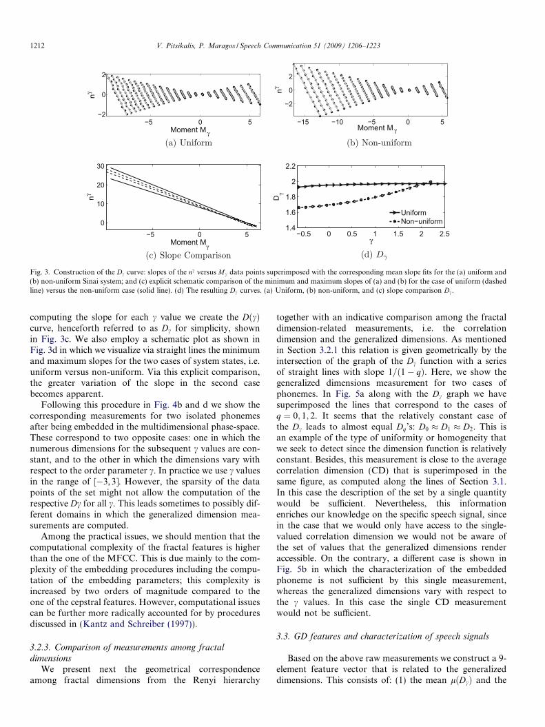


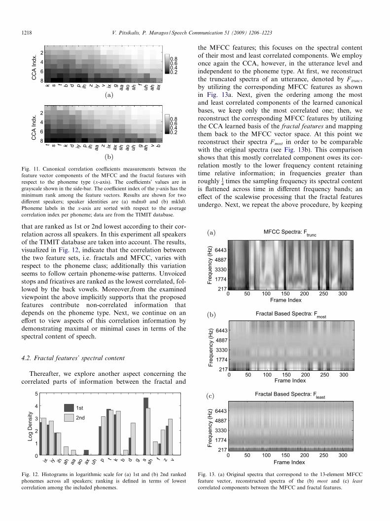


![Denoising Speech Signals for Digital Hearing Aids: A ... book paper.pdfDenoising Speech Signals for Digital Hearing Aids: A Wavelet Based Approach 3 by 2005 (Kochkin[42]). Nevertheless,](https://static.documents.pub/doc/80x56/5fccaba38fdfc244a37a5b45/denoising-speech-signals-for-digital-hearing-aids-a-book-paperpdf-denoising.jpg)


