PROCEEDINGS, 41st Workshop on Geothermal Reservoir Engineering

Stanford University, Stanford, California, February 22-24, 2016

SGP-TR-209

1

Analysis and Interpretation of Stress Indicators in Deviated Wells of the Coso Geothermal Field

Martin Schoenball1,2

, Jonathan M.G. Glen2, Nicholas C. Davatzes

1

1 Earth and Environmental Science, Temple University, 1901 N 13th Street, Philadelphia, PA, 19122, USA, 2 GMEG Science Center, U.S. Geological Survey, 345 Middlefield Road, Menlo Park, CA, 94025, USA

mschoenball@usgs.gov

Keywords: Coso Geothermal Field, stress field, inclined boreholes

ABSTRACT

Characterizing the tectonic stress field is an integral part of the development of hydrothermal systems and especially for enhanced

geothermal systems (EGS). With a well characterized stress field the propensity of fault slip on faults with known location and

orientation can be identified. Faults that are critically oriented for faulting with respect to the stress field are known to provide natural

fluid pathways. A high slip tendency makes a fault a likely candidate for reactivation during the creation of an EGS. Similarly, the stress

state provides insight for the potential of larger, damaging earthquakes should extensive portions of well-oriented, larger faults be

reactivated.

The analysis of stress indicators such as drilling-induced fractures and borehole breakouts is the main tool to infer information on the

stress state of a geothermal reservoir. The standard procedure is applicable to sub-vertical wellbore sections and highly deviated sections

have to be discarded. However, in order to save costs and reduce the environmental impact most recent wells are directionally drilled

with deviations that require appropriate consideration of the deviated trajectory. Here we present an analysis scheme applicable to

arbitrary well trajectories or a combination of wells to infer the stress state. Through the sampling of the stress tensor along several

directions additional information on the stress regime and even relative stress magnitudes can be obtained.

We apply this method on image logs from the pair of wells 58-10 and 58A-10 that were drilled from the same well pad. Both wells have

image logs of about 2 km of their trajectories that are separated by less than 300 m. For both wells we obtain a mean orientation of SHmax

of N23° with large standard deviations of locations of stress indicators of 24° and 26°, respectively. While the local stress direction is

highly variable along both wells with dominant wavelengths from around 50 to 500 m, the mean directions are very consistent and also

agree with previous stress estimates in the eastern part of the Coso Geothermal Field. In order to obtain a reliable estimation of the stress

orientation in this setting, it is necessary to sample the stress field on an interval long to capture several of the dominant wavelengths.

1. INTRODUCTION

The tectonic stress field has a crucial role in the performance of hydrothermal systems and the potential for reservoir engineering for

enhanced geothermal systems and hydrocarbon systems. It has been shown, that critically stress faults provide fluid pathways [Barton et

al., 1995]. These faults are the most likely to become reactivated by hydraulic stimulation, e.g. during the creation of an enhanced

geothermal system. Hence, identification of faults with a high tendency to slip can improve forecasts of the stimulated volume achieved

by hydraulic stimulation and provide insights on the flowpaths in a reservoir. Hence, characterizing the tectonic stress field is an

fundamental task for the characterization of a geothermal system.

At the Coso Geothermal Field considerable efforts have already been made to characterize the stress field. Previous studies of stress

indicators interpreted in borehole image logs [Sheridan and Hickman, 2004; Davatzes and Hickman, 2006, 2010; Blake and Davatzes,

2011] were restricted to sub-vertical sections of the wells and with the commonly made assumption of the vertical stress being a

principal stress direction. In this setting, the location of stress indicators such as borehole breakouts (BO), drilling-induced fractures

(DIF) and petal centerline fractures along the borehole wall are directly related to the orientation of principal stresses in a geographic

coordinate system. This is not true for wells inclined by more than about 12° to a principal stress, where the location of stress indicators

is a highly non-linear function of the relative magnitudes of the principal stresses and the orientation of the borehole with respect to the

local stress tensor [Mastin, 1988]. Since the majority of recently drilled wells at the Coso Geothermal Field were directionally drilled

with deviations in excess of 20° it is of great importance to be able to include these wells in the stress characterization. Furthermore,

aside from earthquake focal mechanisms, the majority of stress measurements collected in the World Stress Map [Heidbach et al., 2010]

stem from analysis of stress indicators in boreholes.

Here, we present a framework for the analysis of deviated sections of well using a grid search over all stress magnitude states permitted

by Mohr-Coulomb faulting [Zoback et al., 2003] and all stress orientations in a frictionally limited Andersonian stress model. The best-

fitting stress state is given by the minimal misfit between the observed orientation of borehole failures and their predicted orientation

according to the assumed stress field. We apply our framework to two pairs of wells that were directionally drilled from the same well

pads. Borehole stress indicators were interpreted from electrical and acoustic wellbore logs. We test whether wells sharing the same

well pad sample the same stress field and discuss the requirements to representatively sample a tectonic stress state using wellbore

failure.

Schoenball et al.

2

2. INTERPRETATION OF INCLINED WELLS

The elastic solutions for the stress field around a cylindrical opening [Kirsch, 1898] predicts compressive stress along the circumference

of wellbores to be largest at azimuths aligned with the minimum stress direction, leading to the formation of borehole breakouts. These

were first observed and used for analysis of the direction of the stress field in the Earth’s crust by Bell and Gough [1979]. Similarly,

tensile stress is observed along the borehole wall at azimuths aligned with the maximum compressive stress that lead to tensile failure of

the borehole wall. Today, the analysis of breakouts and drilling-induced tensile features are a standard procedure in well log analysis

[Zoback et al., 2003; Schmitt et al., 2012]. The standard analysis of borehole failure implicitly assumes that the wellbore axis coincides

with one principal stress direction. In practice, the vertical stress component Sv is assumed to coincide with one principal stress

component. Assuming one principal stress direction is vertical, the effect of wellbore inclination can be neglected for wells that do not

deviate more than about 12° from the vertical [Mastin, 1988]. If the well is inclined with respect to the principal axes of the stress field,

the axis of wellbore failure does not coincide with the wellbore axis anymore. Instead, the location of BOs and DIFs along the borehole

wall is dependent on the magnitudes of the principal stresses and the angle of the wellbore to the principal stress axes. Thus,

interpretation of the direction of horizontal stresses becomes non-unique and dependent on the principal stress magnitudes.

This forward problem was solved by Mastin [1988] and Peška and Zoback [1995]) and various complex inversion schemes for the non-

linear inverse problem have been developed [Qian and Pedersen, 1991; Zajac and Stock, 1997; Thorsen, 2011]. Since deviated

boreholes typically sample the stress tensor at a variety of relative orientations, the onset and relative position of borehole failure as a

function of deviation could potentially provide constraints on stress magnitudes. The underlying assumption of such an approach is that

the remote directions and ratios among the principal stresses are constant throughout the sampled volumes [Wiprut et al., 1997].

Similarly, information from several nearby inclined wells can be combined to constrain stress magnitudes, assuming that all wells

considered are subject to the same stress field [Aadnoy, 1990]. Inversion schemes find the best-fitting stress tensor, but generally the

resolution for general stress states is poor due to noise introduced by heterogeneity of the rock mass. These schemes typically do not

provide feedback on how well the best-fitting solution is constrained by the data either. Therefore, it is difficult to assess the robustness

of the stress states inferred from these schemes. We use a manual grid search approach to stress analysis of inclined wells to gain better

insight into relative fit of stress states to the borehole data and thus a basis for the robustness of the resulting stress model.

2.1 Stress in inclined wellbores

Stresses around a wellbore oriented orthogonally to principal stresses were derived by Kirsch [1898] for plain strain conditions. At the

wellbore wall, they can be simplified to:

𝜎𝜃𝜃 = 𝑆ℎ𝑚𝑖𝑛 + 𝑆𝐻𝑚𝑎𝑥 − 2(𝑆𝐻𝑚𝑎𝑥 − 𝑆ℎ𝑚𝑖𝑛) cos 2𝜃 − 2𝑝0 − Δ𝑝

𝜎𝑟𝑟 = Δ𝑝

𝜎𝑧𝑧 = 𝑆𝑣 − 2𝜈(𝑆𝐻𝑚𝑎𝑥 − 𝑆ℎ𝑚𝑖𝑛) cos 2𝜃 − 𝑝0

(1)

with the maximum and minimum horizontal stresses 𝑆𝐻𝑚𝑎𝑥 and 𝑆ℎ𝑚𝑖𝑛, respectively, the vertical stress 𝑆𝑣, Poisson’s ratio 𝜈 and Δ𝑝 is

the effective mud (fluid) pressure acting on the wellbore wall, i.e. the difference between the mud pressure and the pore pressure in the

formation 𝑝0. The angle 𝜃 is measured clockwise from the direction of 𝑆𝐻𝑚𝑎𝑥. The hoop stress 𝜎𝜃𝜃 reaches a maximum in the direction

of 𝑆ℎ𝑚𝑖𝑛, leading to the formation of breakouts if a failure criterion is met. The minimum of 𝜎𝜃𝜃 is reached in the direction of 𝑆𝐻𝑚𝑎𝑥

and tensile cracks may form at the wellbore wall if the tensile strength of the rock is overcome. The solutions for a more general case,

valid for wellbores inclined with respect to the stress tensor, have been derived by Hiramatsu and Oka [1968].

In the general case, the wellbore axis is not parallel to a principal stress direction and the principal stresses acting on the borehole wall

prescribe an angle with the wellbore axis. To obtain the stress tensor 𝑺𝒃 in the coordinate system parallel to the wellbore axis the first

step is to obtain the stress components 𝑺𝒈 in a geographic coordinate system from the principal components of the stress tensor 𝑺𝒔

[Peška and Zoback, 1995]. This is found using a tensor rotation:

𝑺𝒃 = 𝑹𝒃𝑹𝒔𝑻𝑺𝒔𝑹𝒔𝑹𝒃

𝑻, (2)

where 𝑹𝒔 is the rotation matrix from the coordinate system defined by the principal stresses to the geographic coordinate system and 𝑹𝒃

is the rotation matrix from the geographic the coordinate system to the borehole coordinate system with reference frame defined by the

borehole axis and high side [Peška and Zoback, 1995]. Then, the effective principal stresses acting on the borehole wall are given by

𝜎𝑡𝑚𝑎𝑥 = 1

2(𝜎𝑧𝑧 + 𝜎𝜃𝜃 + √(𝜎𝑧𝑧 − 𝜎𝜃𝜃)2 + 4𝜏𝜃𝑧

2 )

𝜎𝑡𝑚𝑖𝑛 = 1

2(𝜎𝑧𝑧 + 𝜎𝜃𝜃 − √(𝜎𝑧𝑧 − 𝜎𝜃𝜃)2 + 4𝜏𝜃𝑧

2 )

𝜎𝑟𝑟 = Δ𝑝

(3)

where 𝜎𝑧𝑧, 𝜎𝜃𝜃 and 𝜏𝜃𝑧 are the effective stresses in the cylindrical coordinate system of 𝑺𝒃 along an arbitrarily oriented wellbore [Peška

and Zoback, 1995]. The hoop stress 𝜎𝜃𝜃 and the shear stress along the borehole wall 𝜏𝜃𝑧 vary along the azimuth of the well and are not

simple functions of the principal stress azimuths anymore. Borehole breakouts occur where 𝜎𝑡𝑚𝑎𝑥 is above the strength of the rock

Schoenball et al.

3

formation and tensile failure occurring where 𝜎𝑡𝑚𝑖𝑛 is below the tensile strength of the rock. The locations of the extrema represented by

𝜎𝑡𝑚𝑎𝑥 and 𝜎𝑡𝑚𝑖𝑛 are dependent on the relative magnitudes of the principal stresses and vary strongly between stress regimes if the

wellbore deviation is larger than about 12° [Mastin, 1988]. The dependence of the location of extrema of the hoop stress on the relative

stress magnitudes is highly non-linear. Specifically, the locations of stress indicators in a geographic reference frame are not directly

related to the orientation of the stress tensor. For the subsequent analysis, we reference stress indicators to the high side of the well (i.e.

the highest point along a circumference) as opposed to north, which is usually used as reference for the analysis of vertical wells.

2.2 Grid search for best-fitting stress state

Assuming that compressive failure in the Earth’s crust is described by the Mohr-Coulomb criterion and tensile failure occurs when the

pore fluid pressure is above the least principal stress, all equilibrium stress states are bounded by a polygon given by [Zoback et al.,

2003]:

𝑆ℎ𝑚𝑖𝑛 ≥ 𝑆𝑣 − 𝑝

(√𝜇2 + 1 + 𝜇)2 + 𝑝

𝑆𝐻𝑚𝑎𝑥 ≤ (√𝜇2 + 1 + 𝜇)2

(𝑆𝑣 − 𝑝) + 𝑝

𝑆𝐻𝑚𝑎𝑥 ≤ (√𝜇2 + 1 + 𝜇)2

(𝑆ℎ − 𝑝) + 𝑝

(4)

with the coefficient of friction 𝜇. Here, cohesion is assumed to be negligible. The Andersonian stress regimes [Anderson, 1951], with

the vertical stress being one principal stress, as part of the polygon of stress states are then defined by triangles with normal faulting

(NF) for Sv ≥ SHmax ≥ Shmin, strike-slip faulting (SS) for SHmax ≥ Sv ≥ Shmin and thrust faulting (TF) for SHmax ≥ Shmin ≥ Sv.

Figure 1: Polygon of stress states allowed by the Mohr-Coulomb criterion and hydraulic fracturing. Stress states marked by a

gray dot are sampled in our grid search.

In our grid search, we sample all stress states that fall within the polygon on a regular grid (Figure 1). We chose a high value of 1 for 𝜇

to account for all possible stress states. Values higher than that are typically not observed. Similarly, for pore pressure p we assume a

very low value of 0.37 Sv, corresponding to a fluid density of 1000 kg/m3 and an overburden density of 2700 kg/m3. All stress states are

normalized by the vertical stress magnitude Sv which defines the natural scale for stress states that we use throughout this paper. We

implicitly assume constant stress gradients for all principal stresses and pore pressure along the vertical direction. This assumption

might not be permitted in areas with strata that act as fluid barrier or show pronounced rheology. For example, inter-bedding of

argillaceous formations that exhibits a pronounced rheology contrast evidenced by differential creep and stress relaxation can lead to

variable stress gradients [Wileveau et al., 2007]. Hydraulic compartments created by cap rock layers may create over- and

underpressured zones encountered in hydrocarbon systems. However, in the crystalline rock formation that we deal with here a stress

decoupling that leads to variable stress gradients is not expected. Similarly, anomalous pore pressure gradients have not been reported in

the Coso Geothermal Field [Davatzes and Hickman, 2006]. For our analysis we need to infer the location along the borehole wall of the

maximum and minimum of 𝜎𝑡𝑚𝑎𝑥 and 𝜎𝑡𝑚𝑖𝑛, respectively.

For each observed wellbore feature, we compute the angular difference between the observed location and the expected location of that

feature according to equation (3) for all Andersonian stress states and for all orientations of SHmax between N0°E and N179°E. We sum

the absolute misfits for all stress indicators. To account for the different lengths of stress indicators, we weighted the individual misfit of

each indicator according to feature length. Note that we assume Sv to be one principal stress component. This is the same assumption

that is implicitly made during the standard interpretation of vertical wells. We can then draw maps of the stress polygon of (1) the

minimal misfit for each stress state for any stress orientation and of (2) the orientation of SHmax for which that minimal misfit is obtained.

Depending on the well trajectories and the occurrence of stress indicators, we sample the stress tensor along multiple directions along a

single well or by combining picks along several wells with complementary trajectories. For single wells the implicit assumption is that

Schoenball et al.

4

the entire well is in the same stress state. Consequently, for combinations of several wells it is implicitly assumed that the same stress

state is valid for all these wells.

2.3 Data

For our analysis we use two pairs of wells that each share a well pad. The wells 58-10 and 58A-10 (wellheads at 35.999°N, 117.740°W)

are located east of the Coso Wash fault that bounds the currently produced Coso Geothermal Field to the east (Figure 2). They were

drilled in 1997 and 2001, respectively, to potentially extend the producing field to the east. At the writing of this manuscript, the

immediate vicinity has not shown significant levels of seismicity and we assume that the wells sampled an unperturbed natural stress

state. The well 58-10 was drilled sub-vertical to about 1200 m and then deviated by up to 42° towards the NNE direction (Figure 2 and

Figure 3b-c). Well 58A-10 was drilled from the same well pad in a sub-vertical trajectory to 3100 m measured depth (MD). The

deviation does not exceed 10° with exception of the last ~100 m (Figure 2a and Figure 4b-c). Both wells were logged with

Schlumberger’s FMI tool in the upper 12.25 inch sections and with the FMS tool in the lower 8.5 inch sections during drilling breaks.

Additionally, well 58A-10 was logged with an acoustic ALT ABI85 tool in the deep section (Table 1). Despite the strong deviation of

58-10, the well trajectories sample a much larger vertical extent (~2 km) than the lateral extent of the well trajectories (~0.3 km). It is

thus reasonable to expect that both wells sample similar stress fields and both are subjected to similar changes in the stress field at

greater depth. Both wells show an abundance of DIFs along most sections of the well. Specifically, the highly deviated sections of 58-10

exhibit a very large number of DIFs. These contain valuable information that had to be discarded in earlier analyses, which were limited

to sub-vertical sections [Blake and Davatzes, 2011]. Since BOs are very difficult to interpret from electrical logs, we only observe clear

breakouts in the deep section of the 58A-10 well which was logged with the acoustic ABI85 tool. We plot the interpreted stress

indicators with respect to the high side of the well along its circumference, since for deviated wells the inferred direction of the stress

tensor is not directly related with the occurrence of borehole failure in a geographical reference frame. Instead, the high side of the

wellbore wall is used to define the reference frame.

The other pair of wells is 52A-7 drilled in 1991 and 52B-7 drilled in 1992 to expand the produced geothermal field to the west. Their

wellheads are located at 36.040°N, 117.807°W; 7.1 km NW of well pad 58-10. While several other wells were in production near the

well pad, only minor amounts of seismicity were recorded prior to the drilling of these wells [Hauksson et al., 2012]. They were drilled

with a southward trajectory for well 52A-7 and a northward trajectory for well 52B-7 (Figure 2b). Of well 52A-7 only a 155 m long

interval with a 12.5 inch diameter and a deviation on the order of 32° was logged with a FMS tool. The resulting angular coverage is

poor and the tool did not rotate but was probably locked in a borehole enlargement. Well 52B-7 was logged for a 169 m interval using

an FMI tool providing about 70% angular coverage of the 8.75 inch diameter well. Both wells have abundant DIFs with some breakouts

in 52B-7 (Figure 5).

(a) (b)

Figure 2: Trajectories of wells (a) 58-10 and 58A-10 and (b) 52A-7 and 52B-7 with colored sections corresponding to the

acquired image logs analyzed here.

Schoenball et al.

5

(a) (b) (c) (d)

Figure 3: Distribution of stress indicators interpreted in well 58-10. (a) Location of DIFs (red) along the borehole wall

referenced to the high side of the well. (b) Deviation and (c) hole azimuth of the well. (d) Local (along the wellbore) misfit

between the expected location of borehole failure (based on the overall mean stress orientation of N23°E and using the

best-fitting stress magnitude state, see description below) and the actual location of observed failure (red is DIFs). The

gray line is a median-filtered local stress orientation.

(a) (b) (c) (d)

Figure 4: Distribution of stress indicators interpreted in well 58A-10, same as Figure 3. Green features are breakouts with the

line representing the angular extent along the borehole wall.

Schoenball et al.

6

(a) (b) (c) (d)

Figure 5: Distribution of stress indicators interpreted in wells 52A-7 (top half) and 52B-7 (bottom half), same as Figure 4. The

best-fitting stress state is found for both wells simultaneously as described in Section 3.2.

3. RESULTS

Well Log

type

Logged

interval

[m MD]

Typical

deviation

direction

Typical

deviation

Total length

DIFs

[m]

Total

length BOs

[m]

Standard

deviation

[°]

SH,max

orientation

WSM

Quality

52A-7 FMS* 759-914 N200°E 32° 35 0 6 N0°E –

N25°E C

52B-7 FMI* 2552-2721 N340°E 11° 53 5 17 N178°E B

52A-7 &

52B-7 88 5 21 N2°E C

58-10 FMI*

FMS*

145-1584

1584-2142 N30°E 0-30° 139 0 26 N23°E D

58A-10

FMI*

FMS*

ABI85†

583-1975

1982-3055

2070-3118

N320°E <10° 151 24 24° N23°E C

Table 1: Overview of analyzed logs, logged well trajectories and picked stress indicators and inferred orientation of SHmax.

Image log types are: * electric and † acoustic. The number of feature picks refers to single-sided picks.

3.1 Wells 58-10 and 58A-10

We present the results of our grid search as maps drawn on the stress polygon of sampled stress states. The obtained distribution of the

misfit between observed and modeled positions of failure structures in the borehole wall and the best-fitting SHmax orientation over the

sampled stress states are shown in Figure 6. Being a near-vertical well, 58A-10 does not show any strong indication or preference for a

particular stress state. The minimal misfit along all Andersonian stress states is fairly constant (Figure 6b). This is an expected result,

since the standard analysis of vertical wells cannot distinguish between stress regimes from the position of BO and DIFs alone.

However, the best-fitting SHmax orientation varies only minimally between N21°E and N23°E across the tested stress states (Figure 6e).

This variation is much smaller than the standard deviation of the location of stress indicators around the mean orientation, which is 24°.

Well 58-10 has a considerable number of stress indicators in strongly deviated sections. It therefore samples the stress tensor in different

directions – along the vertical direction in the shallow section and along a NNW trajectory deviated by about ~30°. This added

information provides an opportunity to constrain the stress state. The minimal misfit map strongly rejects a thrust faulting regime and

favors all SS stress states and NF stress states with SHmax close to Sv (Figure 6a). The inferred stress orientations for these stress states

agree well with that inferred from well 58A-10 (Figure 6d-e). The variation in best-fitting stress orientations between the two wells for

the preferred stress states is within 5° (Figure 7).

Schoenball et al.

7

If we assume that both wells sample the same stress tensor, we can combine the stress indicator picks for both wells and search for a

single best-fitting stress state valid for both wells. Since the trajectory of 58A-10 does not add directions to the sample that is not

already contained in the sampling along well 58-10 the misfit and orientation maps for both wells do not differ significantly from that of

well 58-10 alone. Only the best-fitting stress orientation for TF stress states takes a value intermediate between that of the two wells

when analyzed separately. Since TF stress states are rejected by their relatively large misfit, this difference of the SHmax orientation has

no physical meaning.

(a) (b) (c)

(d) (e) (f)

Figure 6: Maps of (a-c) Minimum angular misfit summed up and normalized for all stress indicators along Andersonian stress

states, (d-f) Best-fitting orientation of SHmax along all Andersonian stress states. Stress state in wells 58-10 and 58A-10 and

in a combined analysis.

Figure 7: Angular misfit between observed stress indicators and the best-fitting stress orientations for wells 58-10 and 58A-10 as

shown in Figure 6.

3.2 Wells 52A-7 and 52B-7

From the interpreted stress indicators of well 52A-7 most TF and low stress NF regimes can be rejected (Figure 8a). The orientation of

the best-fitting SHMax shows a complex pattern ranging from N15°E for NF stress states to N0°E for SS stress states close to Shmin = Sv.

Additionally, there is a second mode of the best stress orientation for stress states around Shmin = 0.8 Sv, SHMax = 1.8 Sv, corresponding to

Schoenball et al.

8

a SHMax orientation of N25°E (Figure 8d). In this well, a lack of tool rotation resulting in only partial imaging of the borehole

circumference and thus incomplete sampling of the positional variation of the failure structures along the borehole circumference as

well as relatively sparse sampling along the well. For that reason the sampling of the orientation of stress indicators is biased, leading

e.g. to a very narrow distribution of features with an unusually small standard deviation of only 6° (Figure 10c). Without additional

information we cannot further constrain the orientation of the stress tensor. The logged section of well 52B-7 has a relative small

deviation of around 11° and consequently the interpreted BOs and DIFs do not strongly require a particular stress regime. However, the

least misfit is obtained for SS stress states (Figure 8b) and the orientation of SHMax is N178°E.

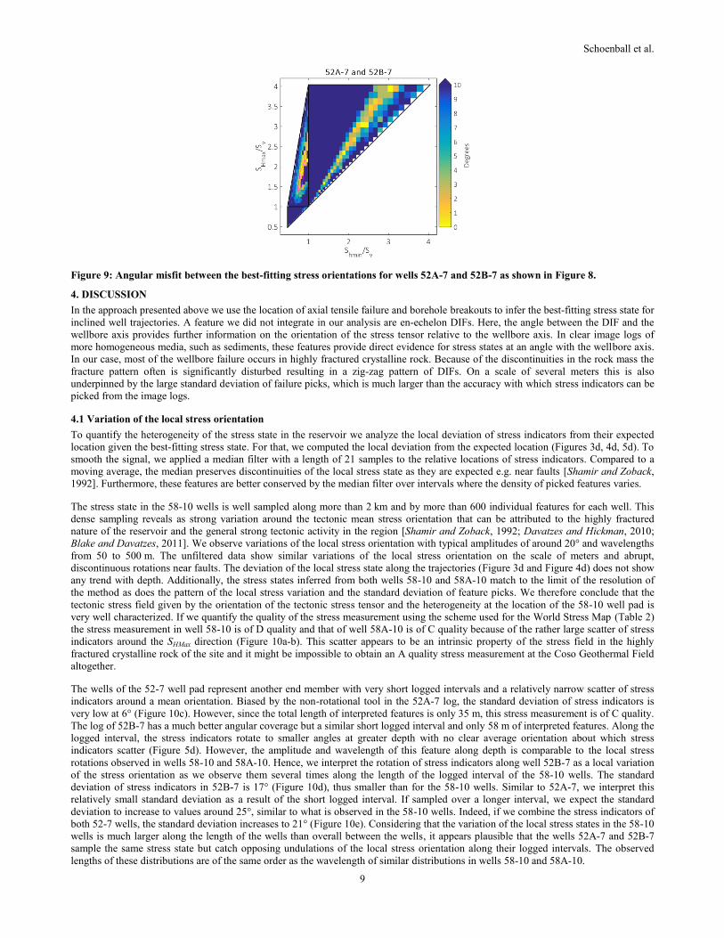
In the next step we combine the picks of stress indicators for both wells to search for a single stress state fitting stress indicators

interpreted in both wells taking advantage of their distinct trajectories. We find that a relatively narrow band of SS stress states is

preferred (Figure 8c) where SHMax = 4.67 Shmin – 2.09 Sv and 0.74 Sv < Shmin < 0.92 Sv (black contour in Figure 8c). These are also the

stress states where the difference of SHMax directions inferred from the wells individually is minimal (Figure 9). The best-fitting

orientation of SHmax for both wells is N2°E (Figure 8f).

While the variation of stress indicators around the obtained mean orientation (Figure 5d) is much larger than for the individual logs, it is

of similar degree as expected when sampling the stress state along wells 58-10 or 58A-10 along 150 m long intervals that are about

1.5 km apart (Figure 10). The obtained standard deviation of 21° is even smaller than the standard deviation of stress indicators found in

the 58-10 wells (Table 1).

(a) (b) (c)

(d) (e) (f)

Figure 8: (a-c) Minimum angular misfit for all stress indicators along Andersonian stress states; the contour in (c) highlights the

best-fitting stress state. (d-f) Best-fitting orientation of SHmax along all Andersonian stress states. Stress state in wells 52A-

7 and 52B-7 and in a combined analysis.

Schoenball et al.

9

Figure 9: Angular misfit between the best-fitting stress orientations for wells 52A-7 and 52B-7 as shown in Figure 8.

4. DISCUSSION

In the approach presented above we use the location of axial tensile failure and borehole breakouts to infer the best-fitting stress state for

inclined well trajectories. A feature we did not integrate in our analysis are en-echelon DIFs. Here, the angle between the DIF and the

wellbore axis provides further information on the orientation of the stress tensor relative to the wellbore axis. In clear image logs of

more homogeneous media, such as sediments, these features provide direct evidence for stress states at an angle with the wellbore axis.

In our case, most of the wellbore failure occurs in highly fractured crystalline rock. Because of the discontinuities in the rock mass the

fracture pattern often is significantly disturbed resulting in a zig-zag pattern of DIFs. On a scale of several meters this is also

underpinned by the large standard deviation of failure picks, which is much larger than the accuracy with which stress indicators can be

picked from the image logs.

4.1 Variation of the local stress orientation

To quantify the heterogeneity of the stress state in the reservoir we analyze the local deviation of stress indicators from their expected

location given the best-fitting stress state. For that, we computed the local deviation from the expected location (Figures 3d, 4d, 5d). To

smooth the signal, we applied a median filter with a length of 21 samples to the relative locations of stress indicators. Compared to a

moving average, the median preserves discontinuities of the local stress state as they are expected e.g. near faults [Shamir and Zoback,

1992]. Furthermore, these features are better conserved by the median filter over intervals where the density of picked features varies.

The stress state in the 58-10 wells is well sampled along more than 2 km and by more than 600 individual features for each well. This

dense sampling reveals as strong variation around the tectonic mean stress orientation that can be attributed to the highly fractured

nature of the reservoir and the general strong tectonic activity in the region [Shamir and Zoback, 1992; Davatzes and Hickman, 2010;

Blake and Davatzes, 2011]. We observe variations of the local stress orientation with typical amplitudes of around 20° and wavelengths

from 50 to 500 m. The unfiltered data show similar variations of the local stress orientation on the scale of meters and abrupt,

discontinuous rotations near faults. The deviation of the local stress state along the trajectories (Figure 3d and Figure 4d) does not show

any trend with depth. Additionally, the stress states inferred from both wells 58-10 and 58A-10 match to the limit of the resolution of

the method as does the pattern of the local stress variation and the standard deviation of feature picks. We therefore conclude that the

tectonic stress field given by the orientation of the tectonic stress tensor and the heterogeneity at the location of the 58-10 well pad is

very well characterized. If we quantify the quality of the stress measurement using the scheme used for the World Stress Map (Table 2)

the stress measurement in well 58-10 is of D quality and that of well 58A-10 is of C quality because of the rather large scatter of stress

indicators around the SHMax direction (Figure 10a-b). This scatter appears to be an intrinsic property of the stress field in the highly

fractured crystalline rock of the site and it might be impossible to obtain an A quality stress measurement at the Coso Geothermal Field

altogether.

The wells of the 52-7 well pad represent another end member with very short logged intervals and a relatively narrow scatter of stress

indicators around a mean orientation. Biased by the non-rotational tool in the 52A-7 log, the standard deviation of stress indicators is

very low at 6° (Figure 10c). However, since the total length of interpreted features is only 35 m, this stress measurement is of C quality.

The log of 52B-7 has a much better angular coverage but a similar short logged interval and only 58 m of interpreted features. Along the

logged interval, the stress indicators rotate to smaller angles at greater depth with no clear average orientation about which stress

indicators scatter (Figure 5d). However, the amplitude and wavelength of this feature along depth is comparable to the local stress

rotations observed in wells 58-10 and 58A-10. Hence, we interpret the rotation of stress indicators along well 52B-7 as a local variation

of the stress orientation as we observe them several times along the length of the logged interval of the 58-10 wells. The standard

deviation of stress indicators in 52B-7 is 17° (Figure 10d), thus smaller than for the 58-10 wells. Similar to 52A-7, we interpret this

relatively small standard deviation as a result of the short logged interval. If sampled over a longer interval, we expect the standard

deviation to increase to values around 25°, similar to what is observed in the 58-10 wells. Indeed, if we combine the stress indicators of

both 52-7 wells, the standard deviation increases to 21° (Figure 10e). Considering that the variation of the local stress states in the 58-10

wells is much larger along the length of the wells than overall between the wells, it appears plausible that the wells 52A-7 and 52B-7

sample the same stress state but catch opposing undulations of the local stress orientation along their logged intervals. The observed

lengths of these distributions are of the same order as the wavelength of similar distributions in wells 58-10 and 58A-10.

Schoenball et al.

10

We therefore suggest considering alternative criteria to assess the quality of stress measurements. Besides the number and cumulative

length of stress indicators and their standard deviation, other critical parameters for the quality of stress measurements are the length of

the interval that is sampled using stress indicators and the absence of a trend over that length, i.e. an absence of a stress rotation with

depth. With the current quality ranking used by the World Stress Map, the stress determination we trust the least (52B-7) yields a B-

quality flag, whereas the stress measurements with the best characterization yields D-quality due to the large intrinsic scatter of stress in

the fractured reservoir.

(a) 58-10 (b) 58A-10

(c) 52A-7 (d) 52B-7 (e) 52A-7 and 52B-7

Figure 10: Rose diagram of stress indicators (BOs and DIFs) transformed to a geographic coordinate system as they would

occur in vertical wells. The light shaded area marks one standard deviation to both sides of the best-fitting mean stress

orientation.

4.2 Integration in a stress model for the Coso Geothermal Field

The orientation of stress indicators and well trajectories of the 58-10 wells constrain the stress regime to SS or high-stress NF regimes,

rejecting NF regimes with low values for SHMax and Shmin and also all TF stress states. The combination of stress indicators of both 52-7

wells prefers a SS stress state around SHMax = 1.8 Sv and Shmin = 0.8 Sv.

Using hydrofrac tests performed in well 38C-9 (wellhead at 36.031°N, 117.776°W, roughly midway between 52-7 and 58-10 well pads

and in a distinct production compartment) Sheridan and Hickman [2004] obtained Shmin = 0.62 Sv, assuming a rock density of

2630 kg/m³. They estimate an upper bound of SHMax from the absence of BOs and assuming a strike-slip stress regime. Then, for a

coefficient of friction of 0.6 to 1.0, they obtain SHMax = 1.2 Sv to 1.9 Sv, respectively. This estimation ignores the thermal effect of the

drilling process, where the well is cooled through circulation of drilling mud, inhibiting compressive failure. Hence, SHMax could still be

above that estimation, which is underpinned by the presence of BOs in the lower section of well 58A-10. Another hydrofrac test

performed in well 34-9RD2 confirmed the low value for Shmin [Davatzes and Hickman, 2006].

The method presented here yields a slightly higher estimate of Shmin than obtained by much more reliable hydrofrac tests. Our estimation

of SHMax is in agreement with the higher end of the range proposed by Sheridan and Hickman [2004] and Davatzes and Hickman [2006].

Both their estimates ignore the thermal effect of the drilling process which could inhibit breakout formation as long as the wellbore is

significantly cooled compared to the unperturbed state. During the logging operations, which occur before a section is cased off, this is

typically the case.

Schoenball et al.

11

Stress

Indicator

A

SHmax believed to be

within ± 15°

B

SHmax believed to be

within ± 15-20°

C

SHmax believed to be

within ± 20-25°

D

Questionable SHmax

orientation (± 25-

40°)

E

no reliable

information (> ± 40°)

Borehole

breakout

≥ 10 distinct breakout

zones and combined

length ≥ 100 m in a

single well with s.d. ≤

12°

≥ 6 distinct breakout

zones and combined

length > 40 m in a

single well with s.d. ≤

20°

≥ 4 distinct breakouts

and combined length

≥ 20 m with s.d. ≤

25°

< 4 distinct breakouts

or < 20 m combined

length in a single well

with s.d. ≤40°

Wells without

reliable breakouts or

s.d. > 40°

Drilling

induced

fracture

≥ 10 distinct fracture

zones in a single well

with a combined

length ≥ 100 m and

s.d. ≤ 12°

≥ 6 distinct fracture

zones in a single well

with a combined

length ≥ 40 m and

s.d. ≤ 20°

≥ 4 distinct fracture

zones in a single well

with a combined

length ≥ 20 m and

s.d. ≤ 25°

< 4 distinct fracture

zones in a single well

or a combined length

< 20 m and s.d. ≤ 40°

Wells without

fracture zones or s.d.

> 40°

Table 2: Excerpt of the World Stress Map quality ranking system version 2008 for the contemporary orientation of maximum

horizontal compressional stress [Heidbach et al., 2010].

5. CONCLUSIONS

The analysis of stress indicators in deviated well sections is a highly non-linear problem. Depending on the well trajectory, the solution

is dependent on an unknown stress magnitude state often requiring additional assumptions or a priori information to find a unique

solution for the best-fitting stress orientation. Because typical wells with a build and hold trajectory sample the stress tensor in different

directions (along the vertical in the shallow parts and along a deviated direction in the bottom part), such wells might actually yield

additional information providing the orientation of the stress tensor and limiting the stress magnitude state to a particular stress regime.

The workflow proposed here provides insight on the way the inferred stress state depends on the relative stress magnitudes.

The interpretation of more than 4 km of image logs of wells 58-10 and 58A-10 provides confidence that inversion of stress indicators in

deviated wells can be successfully applied. The variation of the local stress state along the trajectory of each well is much larger than the

differences of the mean stress directions between the wells that are separated by typically less than 300 m. While the mean stress

direction is N23°E for both wells, the location of stress indicators around a mean direction expected for the mean stress orientation and

the respective trajectory varies with a standard deviation on the order of 25°. This is much larger than the uncertainty of the method,

with picking accuracy on the order of 5° and represents a feature of the local stress state.

We apply these results to the pair of wells 52A-7 and 52B-7 that are logged for short intervals and with a separation of 1.8 km.

Interpreted individually, we would obtain a SHMax orientations of N0°E-N25°E and N0°E for 52A-7 and 52B-7, respectively. However,

if we combine the failure picks of both wells it is reasonable to assume that both wells experience the same stress tensor with an

orientation of SHMax of N2°E. For all wells, a strike-slip stress regime is preferred by the data and the simultaneous interpretation of the

52-7 wells prefers stress states around SHMax = 4.67 Shmin – 2.09 Sv and 0.74 Sv < Shmin < 0.92 Sv. Overall, the direction of SHMax varies

from N23°E at the 58-10 well pad to N2°E at the 52-7 well pad which is 7 km further to the northwest. These well pads are separated by

several geological structures such as the Coso Wash Fault limiting the Coso East Flank to the east and the cold spine separating the East

Flank from the Main Field.

We propose to consider the observed standard deviation of stress indicators a feature of the local stress field. Consequently, they have to

be adequately acknowledged when assigning quality flags to stress measurements. Currently, the number of distinct zones, the

combined length of stress indicators and their standard deviation are used to quantify the quality of stress measurements (Table 2).

However, the length over which these features are sampled is very important to decide if a representative section of the stress field has

been sampled (e.g. the 58-10 logs) or if the logged section only sampled a local undulation of the stress field.

ACKNOWLEDGEMENTS

We acknowledge the support by Navy GPO and Terra-Gen who provided the data. This work is supported by Temple University and the

U.S. Geological Survey’s (USGS) Energy Program’s Geothermal Resource Investigation Project. M. Schoenball is financed by

Cooperative Agreement Number G13AC00283 from the USGS to Temple University: Geothermal Systems in the Western U.S.

REFERENCES

Aadnoy, B. S. (1990), Inversion technique to determine the in-situ stress field from fracturing data, J. Pet. Sci. Eng., 4(2), 127–141.

Anderson, E. M. (1951), The dynamics of faulting and dyke formation with applications to Britain, Oliver and Boyd.

Barton, C. A., M. D. Zoback, and D. Moos (1995), Fluid flow along potentially active faults in crystalline rock, Geology, 23(8), 683–

686.

Bell, J. S., and D. I. Gough (1979), Northeast-southwest compressive stress in Alberta evidence from oil wells, Earth Planet. Sci. Lett.,

45(2), 475–482, doi:10.1016/0012-821X(79)90146-8.

Schoenball et al.

12

Blake, K., and N. C. Davatzes (2011), Crustal stress heterogeneity in the vicinity of the Coso geothermal field, CA, in Stanford

Geothermal Workshop, p. 11.

Davatzes, N. C., and S. H. Hickman (2006), Stress and faulting in the Coso geothermal field: Update and recent results from the East

Flank and Coso Wash, in Stanford Geothermal Workshop, p. 12.

Davatzes, N. C., and S. H. Hickman (2010), The Feedback Between Stress , Faulting , and Fluid Flow: Lessons from the Coso

Geothermal Field, CA, USA, in World Geothermal Congress, pp. 25–29, Bali, Indonesia.

Hauksson, E., W. Yang, and P. M. Shearer (2012), Waveform relocated earthquake catalog for southern California (1981 to June 2011),

Bull. Seismol. Soc. Am., 102(5), 2239–2244, doi:10.1785/0120120010.

Heidbach, O., M. Tingay, A. Barth, J. Reinecker, D. Kurfeß, and B. I. R. Müller (2010), Global crustal stress pattern based on the World

Stress Map database release 2008, Tectonophysics, 482(1-4), 3–15, doi:10.1016/j.tecto.2009.07.023.

Hiramatsu, Y., and Y. Oka (1968), Determination of the stress in rock unaffected by boreholes or drifts, from measured strains or

deformations, Int. J. Rock Mech. Min. Sci. Geomech. Abstr., 5(4), 337–353, doi:10.1016/0148-9062(68)90005-3.

Kirsch, G. (1898), Die Theorie der Elastizität und die Bedürfnisse der Festigkeitslehre, Zeitschrift des Vereins Dtsch. Ingenieure, 42,

797–807.

Mastin, L. (1988), Effect of borehole deviation on breakout orientations, J. Geophys. Res., 93(B8), 9187,

doi:10.1029/JB093iB08p09187.

Peška, P., and M. D. Zoback (1995), Compressive and tensile failure of inclined well bores and determination of in situ stress and rock

strength, J. Geophys. Res., 100(B7), 12791, doi:10.1029/95JB00319.

Qian, W., and L. B. Pedersen (1991), Inversion of borehole breakout orientation data, J. Geophys. Res., 96(B12), 20093,

doi:10.1029/91JB01627.

Schmitt, D. R., C. A. Currie, and L. Zhang (2012), Crustal stress determination from boreholes and rock cores: Fundamental principles,

Tectonophysics, 580, 1–26, doi:10.1016/j.tecto.2012.08.029.

Shamir, G., and M. D. Zoback (1992), Stress orientation profile to 3.5 km depth near the San Andreas Fault at Cajon Pass, California, J.

Geophys. Res., 97(B4), 5059, doi:10.1029/91JB02959.

Sheridan, J. M., and S. H. Hickman (2004), In situ stress, fracture, and fluid flow analysis in well 38C-9: An enhanced geothermal

system in the Coso Geothermal Field, in Stanford Geothermal Workshop, p. 8.

Thorsen, K. (2011), In situ stress estimation using borehole failures — Even for inclined stress tensor, J. Pet. Sci. Eng., 79(3-4), 86–100,

doi:10.1016/j.petrol.2011.07.014.

Wileveau, Y., F. H. Cornet, J. Desroches, and P. Blümling (2007), Complete in situ stress determination in an argillite sedimentary

formation, Phys. Chem. Earth, Parts A/B/C, 32(8-14), 866–878, doi:10.1016/j.pce.2006.03.018.

Wiprut, D., M. Zoback, T.-H. Hanssen, and P. Peška (1997), Constraining the full stress tensor from observations of drilling-induced

tensile fractures and leak-off tests: Application to borehole stability and sand production on the Norwegian margin, Int. J. Rock

Mech. Min. Sci., 34(3-4), 365.e1–365.e12, doi:10.1016/S1365-1609(97)00157-3.

Zajac, B. J., and J. M. Stock (1997), Using borehole breakouts to constrain the complete stress tensor: Results from the Sijan Deep

Drilling Project and offshore Santa Maria Basin, California, J. Geophys. Res., 102(B5), 10083, doi:10.1029/96JB03914.

Zoback, M. D., C. A. Barton, M. Brudy, D. A. Castillo, T. Finkbeiner, B. R. Grollimund, D. B. Moos, P. Peška, C. D. Ward, and D. J.

Wiprut (2003), Determination of stress orientation and magnitude in deep wells, Int. J. Rock Mech. Min. Sci., 40(7-8), 1049–

1076, doi:10.1016/j.ijrmms.2003.07.001.