Analysis and Processing of Mechanically Stimulated Electrical Signals for the Identification of Deformation in Brittle Materials by PANAGIOTIS A. KYRIAZIS A thesis submitted for the degree of Doctor of Philosophy School of Engineering & Design Brunel University, London UNITED KINGDOM January 2010
Transcript
Analysis and Processing of Mechanically Stimulated
Electrical Signals for the Identification of
Deformation in Brittle Materials
by
PANAGIOTIS A. KYRIAZIS
A thesis submitted for the degree of Doctor of Philosophy
School of Engineering & Design
Brunel University, London
UNITED KINGDOM
January 2010
P a g e | 2
Dedicated to my parents and siblings
P a g e | 3
Abstract
The fracture of brittle materials is of utmost importance for civil engineering and
seismology applications. A different approach towards the aim of early identification of
fracture and the prediction of failure before it occurs is attempted in this work.
Laboratory experiments were conducted in a variety of rock and cement based material
specimens of various shapes and sizes. The applied loading schemes were cyclic or
increasing and the specimens were tested to compression and bending type loading of
various levels.
The techniques of Pressure Stimulated Current and Bending Stimulated Current were used
for the detection of electric signal emissions during the various deformation stages of the
specimens. The detected signals were analysed macroscopically and microscopically so as
to find suitable criteria for fracture prediction and correlation between the electrical and
mechanical parameters.
The macroscopic proportionality of the mechanically stimulated electric signal and the
strain was experimentally verified, the macroscopic trends of the PSC and BSC electric
signals were modelled and the effects of material memory to the electric signals were
examined. The current of a time-varying RLC electric circuit was tested against
experimental data with satisfactory results and it was proposed as an electrical equivalent
model.
Wavelet based analysis of the signal revealed the correlation between the frequency
components of the electric signal and the deformation stages of the material samples.
Especially the increase of the high frequency component of the electric signal seems to be
a good precursor of macrocracking initiation point. The additional electric stimulus of a dc
voltage application seems to boost the frequency content of the signal and reveals better
the stages of cracking process. The microscopic analysis method is scale-free and thus it
can confront with the problems of size effects and material properties effects.
The AC conductivity time series of fractured and pristine specimens were also analysed by
means of wavelet transform and the spectral analysis was used to differentiate between the
specimens. A non-destructive technique may be based on these results.
Analysis has shown that the electric signal perturbation is an indicator of the forthcoming
fracture, as well as of the fracture that has already occurred in specimens.
List of Tables ....................................................................................................................................... 7
List of Figures ...................................................................................................................................... 7
Appendix A – Publications derived from this research work .......................................................... 163
Appendix B – Experimental setups, materials and devices ............................................................ 165
P a g e | 7
List of Tables Table 4.1 The parameters that arise from fitting of the PSC signals in every loading cycle according
to equation (4.3.1) and the correlation coefficient showing the fitting accuracy [from Kyriazis et al., 2006] ............................................................................................................................... 82
Table 4.2 The parameters that arise from fitting of the PSC signals in every loading cycle according to equation (4.3.6) and the correlation coefficient showing the fitting accuracy .................... 91
Table 4.3 RLC circuit model component values for four loading steps .......................................... 118
List of Figures
Figure 2.1 (a) Stress in a column as a result of an externally applied force Fext (b) longitudinal and lateral strain in an elongated beam by means of external tensile force. ................................. 19
Figure 2.2 The stages of deformation and fracture of brittle materials in uniaxial stress and the corresponding relationship between stress and strain ............................................................ 21
Figure 2.3 Tensile strength size effect based on Carpinteri 1996 size effect analysis ...................... 24 Figure 2.4 (a) Geometry used for calculations of a sliding crack under compression (b) actual wing
crack and linearly estimated crack with angle depending on length ....................................... 27 Figure 2.5 Axially applied tensile stress to infinite body with crack of 2α length ............................ 30 Figure 2.6 (a) The load on each fibre equals to one fourth of the total load, (b) the load on each
undamaged fibre is one third of the total, (c) each of the remaining fibre carries half of the total load and (d) all fibres have failed - no load is carried ...................................................... 32
Figure 2.7 (a) Time vs. voltage generated by the plain cement paste (4 kN/s) – taken from (Sun M. , Liu, Li, & Hu, 2000) and (b) The electrical emission in mortar (the loading rate is 1 kN/s) – taken from (Sun M. , Liu, Li, & Wang, 2002) ............................................................................. 39
Figure 2.8 (a) Channels 1-3 three ring collector electrodes 500, 100 and 20mV respectively – taken from (Freund F. , 2002) and (b) Example of experimental results – taken from (Takeuchi, 2009) ......................................................................................................................................... 39
Figure 2.9 (A) Experimental data from granite sample (a) applied pressure and (b) differential voltage and (B) experimental data from marble sample (a) applied pressure and (b) differential voltage – taken from (Aydin, Prance, Prance, & Harland, 2009) ........................... 40
Figure 2.10 (a) Time domain amplitude (signal graph – temporal evolution) (b) Frequency domain (Fourier Transform – spectrogram) (c) Short Time Fourier Transform (time localisation of frequency components- equispaced windowed analysis) and (d) Wavelet Transform time scale .......................................................................................................................................... 43
Figure 2.11 The effect of parameter a and b on mother wavelet ψ (the translation and dilation of the mother wavelet with respect to time when parameters a and b increase) ....................... 45
Figure 2.12 The graphs of ψ wavelet functions (plotted in Matlab wavelet toolbox) for (a) the Meyer Wavelet and (b) the Mexican Hat wavelet .................................................................... 47
Figure 2.13 Daubechies wavelet family graphs (plotted in Matlab wavelet toolbox) of ψ wavelet function for the (a) 2nd Daubechies wavelet (b) 3rd Daubechies wavelet, (c) 4th Daubechies wavelet and (d) 10th Daubechies wavelet ................................................................................ 48
Figure 3.1 (a) Specimens were extracted either parallel or perpendicular to borehole axis, the coloured direction of extraction was selected for the experiments, (b) the experimental setup
P a g e | 8
for testing amphibolite samples (c) specimen after failure, diagonal shearing plane – taken from (Triantis, Anastasiadis, Vallianatos, Kyriazis, & Nover, 2007) .......................................... 53
Figure 3.2 Mechanical setup for experiments of mechanically stimulated electric signal identification ............................................................................................................................. 60
Figure 3.3 Screenshot of the control and measurements acquisition software .............................. 61 Figure 3.4 Basic measurement setup of Pressure Stimulated Currents technique .......................... 63 Figure 3.5 Basic measurement setup of Bending Stimulated Currents technique ........................... 64 Figure 3.6 Loading schemes for PSC and BSC experimental techniques .......................................... 65 Figure 3.7 Experimental setup for the evaluation of the amended PSC technique ......................... 68 Figure 3.8 (a) Stress step evolution over time, (b) PSC recording of the two electrometers in
common y-axis. And (c) normalised PSC recordings with and without externally applied DC voltage ....................................................................................................................................... 69
Figure 3.9 PSC signal recordings, macroscopic trends and wavelet scalograms of (a) specimen tested according to conventional PSC technique (b) specimen tested with the amended PSC technique – taken from (Kyriazis, Anastasiadis, Triantis, Stavrakas, Vallianatos, & Stonham, 2009) ......................................................................................................................................... 70
Figure 3.10 Experimental setup for ac conductivity time series measurements ............................. 71 Figure 4.1 (a) Stress and Strain evolution over time in a typical low level loading cyclic
compression test and (b) The equivalent emitted PSC signal by the tested marble specimen 75 Figure 4.2 The unloading process evolution, focusing on (a) the stress and the corresponding
results on (b) strain and (c) PSC signal emission from marble specimen ................................. 76 Figure 4.3 (a) The evolution of strain over time and (b) the corresponding PSC signal in a typical
stress controlled strength test of cement material sample. .................................................... 78 Figure 4.4 (a) Typical stress – strain curve of cement and (b) of marble specimens, (c) PSC signal
evolution over time for cement and (d) for marble specimen ................................................. 79 Figure 4.5 (a) The step-wise applied axial stress (normalised), (b) the corresponding PSC signal
(normalised) and the identification of the two relaxation processes (fast and slow) .............. 81 Figure 4.6 Pressure Stimulated Currents that are emitted by marble sample in three successive
loading cycles, fitted according to equation (4.3.1) [from Kyriazis et al., 2006] ..................... 82
Figure 4.7 The relaxation time factor 2τ for marble and amphibolite over three and four
successive loading cycles respectively. ..................................................................................... 83 Figure 4.8 (a) The applied stress steps (normalised) to cement paste specimen, (b) the calculated
first derivative of the applied stress – stress rate and (c) the corresponding PSC signal recordings for the three steps. ................................................................................................. 84
Figure 4.9 (a) Stress steps applied on marble specimen, (b) the calculated stress rate of each loading cycle and (c) the corresponding PSC signal peaks and relaxation. .............................. 85
Figure 4.10 (a) Stress steps applied on marble specimen, (b) the strain recorded by strain gages, (c) the stress rate evolution over time and (d) the corresponding PSC signal peaks and relaxation. ................................................................................................................................. 87
Figure 4.11 (a) Stress steps applied on amphibolite rock specimen, (b) the stress rate evolution over time and (c) the corresponding PSC signal peaks and relaxation. .................................... 88
Figure 4.12 Pressure Stimulated Current recordings from four repetitive loading steps of the same level and their fitting with Probability Density Function of the Extreme Value distribution ... 92
Figure 4.13 (a) Loading scheme used for three-point bending test on marble beam, (b) the loading rate evolution over time and (c) the corresponding BSC signal peaks and relaxation. ............ 93
P a g e | 9
Figure 4.14 Normalised BSC peaks and total charge that flows past the electrodes at each loading level – taken from (Kyriazis, Anastasiadis, Stavrakas, Triantis, & Stonham, 2009) .................. 95
Figure 4.15 Linearly fitted slow relaxation time factors τ2 of the BSC signals with respect to the normalized loading level and a typical relaxation process and the exponential trend that follows ....................................................................................................................................... 96
Figure 4.16 Normalised Cumulative distribution of charge recorded by the attached to the specimen electrodes versus the normalised loading level – taken from (Kyriazis, Anastasiadis, Stavrakas, Triantis, & Stonham, 2009) ...................................................................................... 98
Figure 4.17 (a) Coordinate system of a beam subjected to bending, (b) Bending in z-y plane, (c) Bending in x-z plane – taken from (Case, Chilver, & Ross, 1999) and (d) Three dimensional presentation of the stress distribution in cross-section plane of a bended beam ................... 99
Figure 4.18 BSC peaks evolution by means of two discrete processes i.e the tension process and the compression process – taken from (Kyriazis, Anastasiadis, Stavrakas, Triantis, & Stonham, 2009) ....................................................................................................................................... 100
Figure 4.19 (a) Applied loading to the FRP sheet, (b) the loading rate of the experimental process and (c) the corresponding BSC signal ...................................................................................... 101
Figure 4.20 (a) BSC signal recordings of 2nd and 3rd loading steps on FRP sheet and (b) normalised BSC signal recordings from cement mortar beams and FRP sheets ....................................... 102
Figure 4.21 Five step-wise loadings of 2mins per step duration and varying relaxation times (a) 4mins (b) 2mins and (c) 1 min, alongside with the corresponding PSC signal ....................... 105
Figure 4.22 The evolution of PSC signal peaks (normalised) over loading cycles for the three experimental parts which are characterised by varying relaxation times .............................. 106
Figure 4.23 The evolution of PSC signal peaks (normalised) over loading cycles for temporary and permanent memory effects on marble and amphibolite respectively ................................... 107
Figure 4.24 Relaxation evolution of the first and the following (2nd to 5th) steps in common time axis, from the experimental data of short memory test on marble (part 2 experiment i.e. 4min relaxation time) .............................................................................................................. 109
Figure 4.25 The delay in PSC peak occurrence during repetitive loading. PSC signal snapshots shifted in time for common time reference t0 presentation, yielding from amphibolite specimen subjected to 4 stress steps. .................................................................................... 111
Figure 4.26 Simultaneous plotting of the response to the initial stress steps for each of the first two parts of short memory effects experiments shown in Figure 4.21 ................................. 112
Figure 4.27 The equivalent RLC circuit that models macroscopically the PSC emission system .... 114 Figure 4.28 The applied stress scheme and the resulting PSC electric signal – taken from
(Anastasiadis, Triantis, & Hogarth, 2007) ............................................................................... 116 Figure 4.29 (a) The PSC recorded during four consecutive loadings of a marble sample and (b) the
equivalent current emitted by an RLC circuit macroscopic model ......................................... 117 Figure 4.30 PSC recorded data against RLC model current in each loading step ........................... 118 Figure 4.31 The equivalent RLC circuit that models macroscopically the PSC emission system .... 119 Figure 5.1 The self-similarity (fractal) of the scaling function of Daubechies 3rd order wavelet... 127 Figure 5.2 (a) The Daubechies 3rd order scaling function and (b) the 3rd order mother wavelet 128 Figure 5.3 (a)Pressure Stimulated Current signal recordings from three successive loading cycles
merged in the same graph, (b)Time scale analysis (scalogram) of the electric signal, resulting from CWT – taken from (Kyriazis, Anastasiadis, Triantis, & Vallianatos, 2006) ...................... 129
P a g e | 10
Figure 5.4 Scalograms yielding from CWT analysis of each part of the signal (a) First step (b) second step and (c) third step – taken from (Kyriazis, Anastasiadis, Triantis, & Vallianatos, 2006) ....................................................................................................................................... 130
Figure 5.5 (a) Increasing step-wise loading scheme applied on cement specimen, (b) the PSC signal emitted as a result of mechanical stimulation of specimen and (c) the CWT resulting scalogram ................................................................................................................................ 132
Figure 5.6 The evolution of PSC signal after the 2nd and 3rd loading steps in time domain and the corresponding scalograms yielding from CWT analysis of the signals using the same parameterisation .................................................................................................................... 133
Figure 5.7 (a) Time domain PSC signal recordings from specimen subject to mechanical loading of variable scheme, level and duration (b) CWT scalogram (2D) analysis of the total PSC signal and (c) the CWT scalogram (3D) expressing the coefficient values by colour and surface perturbation ............................................................................................................................ 135
Figure 5.8 The detrended ac conductivity time series for (a) uncompressed and (b) compressed samples, distribution of detrended conductivity time series for (c) uncompressed and (d) compressed samples – taken from (Kyriazis, Anastasiadis, Triantis, & Stonham, 2006) ........ 138
Figure 5.9 Scalograms yielding from CWT of ac conductivity time series of uncompressed (a), (b), (c) and compressed samples (d), (e), (f), by using Mexican Hat, Daubechies 2nd and Daubechies 10th order, as mother wavelets accordingly – taken from (Kyriazis, Anastasiadis, Triantis, & Stonham, 2006) ..................................................................................................... 139
Figure 5.10 Calculated wavelet power spectra of uncompressed and compressed samples using (a) Mexican Hat, (b) Daubechies 2nd and (c) Daubechies 10th order as mother wavelets accordingly – taken from (Kyriazis, Anastasiadis, Triantis, & Stonham, 2006) ....................... 140
Figure 6.1 (a) Sensor for mechanically stimulated electric signal detection and analysis (b) Sensor subnetwork that ‘resides’ inside a beam subjected to bending and (c) sensor network inside a cement based ‘skleleton’ of a building, which is composed by the subnetworks shown by in columns and beams ................................................................................................................ 149
The unique experience of delving into a specific research field during the PhD would not
have been completed, if it was not for some people that I would like to thank for their help.
First of all, I would like to express my gratitude to my supervisor Prof. John Stonham, who
was a constant source of support and confidence for the outcome of this work. His advices
were always helpful and his experience in the research processes allowed safe and fruitful
steps towards the final aims.
A special thank to my second supervisor Prof. Cimon Anastasiadis for the stimulating
conversations we had during this work. His leniency for my primitively presented ideas
and work, as well as his encouragement during the difficult days of this research, was
beyond any expectation.
I would like to express my deepest gratitude to Prof. Dimos Triantis for guiding me
through the solitary paths of this research. He was always an inspiration for me and an
example to follow as a scientist. I owe him much of what I have achieved during this work,
which was enlightened by his thought-provoking comments.
Many thanks to Prof Filippos Vallianatos, Dr Ilias Stavrakas and Dr Antonis
Kyriazopoulos for helping me confront with theoretical and experimental issues; their
expertise in this research fields was invaluable.
The National Foundation of Scholarships (IKY) in Greece is gratefully acknowledged for
his financial support during this research.
Last but not least, I thank my family for their love, patience and encouragement. I would
not have made it without their support. The least I can do in gratification of their
contribution is to dedicate this work to them.
Mr. Panagiotis A. Kyriazis
January 2010
P a g e | 13
Chapter 1
Introduction
P a g e | 14
1 Introduction
1.1 Motivation and perspectives of research Electronic engineering development and the technological advancements during the last
decades, has led to the infiltration of electronics into every single discipline of research.
Electronics as core technology in mobile communications, computers, nanoelectronics and
artificial intelligence applications have changed everyday life of modern world, but they
have also acted as a powerful enabler for the development of other long-established
sciences. Mechanical and chemical engineering, as well as biology and medicine have been
offered powerful electronic and computer tools that facilitate accuracy, integrity,
minimisation of errors, speed of processing, minimisation of costs, high quality products
and services, sophisticated solutions of complex problems and transfer of human
experience to machines.
Geotechnology and seismology have been benefited by the expansion of computer
networks and datalogging systems as well as of the latest research in satellite based remote
sensing. Civil engineering has been influenced by the advantages of computer parallel
processing and finite element methods to model and solve complex problems. Between the
two aforementioned sciences no evident correlation exists, but they share a common
interest for fracture phenomena and processes.
Looking deeper in their objectives, the two sciences are trying to predict the fracture
occurrence by identifying and evaluating the causes behind it. Civil engineering focuses of
the stresses distribution, tries to predict their values and keep it within tolerance limits,
whereas seismology seeks for geological precursory evidence and periodicity of
phenomena to predict the evolution of crust fracture and therefore the resulting earthquake.
The common fracture properties of brittle construction materials and geomaterials,
alongside with the consensus about the existence of electromagnetic signal which is
precursory to fracture, were the basic motivations of this work. Electric signal can be
detected and measured with accuracy owing to the available devices and sensors and
sophisticated tools for processing of the signal can reveal information that were ‘invisible’
with conventional processing tools.
Therefore a better understanding and more accurate prediction of the fracture based on
localised data and correlation of fracture with respect to its results (i.e. electric signal
emission) instead to its causes, would be beneficial for both sciences. Upon the results of
this core research topic, civil engineering applications such as self-healing buildings and
P a g e | 15
non-destructive testing, as well as the most crucial quest of seismology, i.e. the earthquake
prediction, would obtain long perspectives of development.
1.2 Objectives and contribution of this work The ultimate objective of this work is to correlate the resulting strain and fracture of a
material sample, because of stress application, to the corresponding electric signal
emission. The success of this objective involves primary and secondary aims that are given
concisely below.
Verification of the existence of mechanically stimulated electric signals for a
variety of brittle materials; the universality of brittle fracture induced phenomena.
Comparison between mechanically stimulated electric signals of different
materials to reveal differences and similarities.
Settlement of standard experimental techniques for the detection of mechanically
stimulated electric signal flowing out of brittle material specimens.
Design of mechanical and electrical setup for standard compression and
bending laboratory fracture tests.
Selection of measuring equipment and appropriate measurement settings.
Specification of material, shape and positioning of sensing elements, to
enable signal detection and avoid mutual coupling and signal interference.
Identification of the ambient experimental setup parameters that may affect
the signal; quantification of their influence and minimisation within
acceptable tolerances.
Amendments in the experimental techniques, so as to focus on specific
fracture related properties of the signal.
Analysis of the detected signal and correlation with its mechanical properties.
Noise level analysis and filtering of the signal
Differentiation between the signal that is related to permanent mechanical
deformation and the signal related to dynamic deformation.
Evaluation of the influence of memory and size effects on the signal.
Identification of the signal trends and their correlation to the stage of
deformation and the type of loading.
Identification of the most reliable parameter of the signal to evaluate for
concluding on the deformation it has suffered and its remaining strength.
P a g e | 16
Definition of signal evaluation criteria for the prediction of the forthcoming failure
before the stage of unstable crack evolution.
Testing of various stress modes effect on signal close to fracture region of
the material samples.
Advanced mathematics processing for failure precursory information of the
signal.
In this work we have focus in most of the aforementioned research goals and we have
contributed with some innovative ideas concerning the signal processing and the
experimental techniques.
1.3 Roadmap of the thesis This thesis follows a bottom up approach in the presentation of information. Following to
the initial chapter of introduction, we present in Chapter 2 the basic theoretical knowledge
in the scientific fields that are involved in this multidisciplinary work. We analyse in
separate subsections the mechanical and civil engineering basic ideas that are used for
experiments and for interpretation of data, as well as the related work on the domain of
electric signals triggered by mechanical stimuli, which is conducted by other researchers.
Another subsection of Chapter 2 is dedicated to the advanced mathematical tool of signal
processing known as Wavelet analysis that has been extensively used in this work.
In Chapter 3 we have gathered together the experimental techniques used in this work. We
have referred to the properties of the materials under examination and to the specification
of the measuring systems that have been used. We have presented the experimental
techniques by separating them into two domains the real time and the non-real time. The
former was analysed separately into the two consisting parts i.e. the PSC and the BSC
experimental techniques respectively. The non-real time experimental process has one
representative, namely the ac-conductivity time series experimental technique.
The analysis of the signals recorded by the aforementioned experimental techniques is
presented in Chapters 4 and 5 from the macroscopic and microscopic point of view
respectively. Chapter 4 contains the macroscopic parameters of the PSC and BSC signals
evolution and modelling. It focuses on the trends of the signal during cyclic and increasing
loading and shows the effects of material memory into the signal. It also presents some
comparative analysis between signals of different materials and a framework for the
understanding of electrification mechanisms according to the deformation stages. Chapter
5 is dedicated to microscopic analysis of the signal via the powerful tool of wavelet
P a g e | 17
transform. The signal is depicted in form of scalograms in order to emphasise on its
frequency content. Time-scale analysis of both PSC and BSC signals is presented in this
chapter. A subsection is dedicated to the wavelet analysis results for the differentiation of
pristine and fractured specimens through the evaluation of spectral analysis of ac
conductivity time series.
In Chapter 6 the results of this work are summarised and the guiding lines for the next
research steps are given. Future work that can be based on the outcome of this research is
presented as a triggering for innovative research projects.
P a g e | 18
Chapter 2
Theoretical Background
P a g e | 19
2 Theoretical background
2.1 Introduction This work is multidisciplinary and it involves some basic knowledge of civil engineering
and fracture mechanics, as well as signal processing and wavelets analysis that are mostly
used in electronic engineering for processing and compressing signals. The necessary
background theory for understanding this work ideas and concepts are addressed in the
following sections.
2.2 Fracture mechanics and physical models
2.2.1 Stress and strain basic concepts
Stress is the internal response of a homogenous body to an externally applied force. The
body shown in Figure 2.1a is by hypothesis in a static equilibrium and thus according to
action and reaction principle when an external force Fext is applied the body reacts by an
equivalent force Fint, which acts in the cross sectional area A. The stress σ is given by
equation (2.2.1) in the idealised case that external force is perpendicular to area A.
FA
σ = (2.2.1)
Generally for any force on a specimen other for geometrically regular prism specimens or
for any continuous and homogenous body the external force Fext can be analysed into a
perpendicular force FP and a tangential force FT to the cross sectional plane. These two
forces are used to define the normal stress σ and the shear stress τ, for a specific point just
by minimizing area A to infinitesimal dimensions, as shown in equation (2.2.2).
external force, Fext
Figure 2.1 (a) Stress in a column as a result of an externally applied force Fext (b) longitudinal and lateral strain in an elongated beam by means of external tensile force.
Cross sectional area, A
internal force, Fint
(a) (b)
L
ΔL
d0 d0- Δd
Fext Fext
P a g e | 20
0 0
lim and limP T
A A
F FA A
σ τ→ →
= = (2.2.2)
Both σ and τ vary in a body and depend upon the cross sectional plane orientation in the
point of interest. Therefore the stress is better defined by a stress tensor, which represents
the mean forces acting on an infinitesimal cube that is defined around the point. A more
detailed description of this tensor analysis of stress can be found in (Sanford, 2003).
The result of the stress in a body is the deformation, either contraction in case of
compressive stress or elongation in tensile stress case, as shown in Figure 2.1b. Strain ε is
an absolute number expressing the ratio of the elongation ΔL to the initial length L of the
body, as shown in equation (2.2.3a) and the ratio of the width decrease Δd to the original
width d0, as shown in equation (2.2.3.b). The two expressions of strain are known as the
longitudinal and lateral strain respectively.
0
and εlongitudinal lateralL d
L dε ∆ ∆
= = − (2.2.3)
The ratio expressing strain is usually extremely small and thus values are given in μm/m,
multiplied by a factor of 106.
The relation between stress and strain is a typical cause and effect relation. For low stress
values a linear relation between stress and strain is observed, which is described by the so
called modulus of elasticity Y or Young’s Modulus, named after Thomas Young a pioneer
physicist.
σε
Υ = (2.2.4)
Equation (2.2.4) is the definition of Young’s modulus. As far as a stressed material sample
follows this linear relation known as Hooke’s law of elasticity is considered to be in the
elastic region, as opposed to the plastic region, both regions are shown in Figure 2.2.
The relation between the two different directions of strain are characteristic for each
material and it is expressed by a proportional constant, known as Poisson’s ratio, which is
given by equation (2.2.5).
lateral
longitudinal
v εε
= (2.2.5)
Typical value for Poisson’s ratio of steel and iron is 0.3, for aluminium is 0.34 and for
concrete and rocks is considerably lower at 0.1. These values may be taken into account
for the selection of the specimen dimensions in the experiments.
P a g e | 21
The stress-strain curve can depict graphically the relationship between stress and strain. It
can also give information about the mechanical stages of a material sample and about its
corresponding behaviour. In Figure 2.2 is shown a typical stress-strain curve and the stages
of the mechanical deformation of a brittle material, beginning from the stage that the
material is considered to be pristine up to the stage of failure and collapse. The
experiments that lead to these results are conducted by either increasing the stress
monotonically or by loading in stress relaxation mode, which is equivalent to keep strain
increase constant. The basic stages of the material fracture are briefly explained using the
stress as parameter of control.
i. The first stage is the closing of cracks stage, which corresponds to the initial part of the
stress-strain curve and it is characterised by a quick and non linear increase of strain as
the stress increases. The stress on the material sample leads to the compression and
closing of the inherently present cracks even at a theoretically pristine sample.
ii. The second stage is known as the elastic region of the material, because deformation is
not permanent, if the material sample is subjected to cyclic loading of these stress
levels. Despite the linear relation between stress and strain in this stage, the “elasticity”
in brittle materials is different to this of ductile materials. At a specific stress level of
this stage the pre-existing cracks in the bulk of the material start to propagate. The
propagation is normal, which means that the increase of stress is followed by a stable
Figure 2.2 The stages of deformation and fracture of brittle materials in uniaxial stress and the corresponding relationship between stress and strain in compression
termination of crack closure process
initiation of cracks
end of linear axial deformation
strain (ε)
stress (σ)
ultimate strength
Y=σ/εconstant
P a g e | 22
pace crack propagation and if no stress is further applied the crack propagation stops
(Bieniawski, 1967).
iii. Further increase in the stress level has a severe impact on the strain of the material
sample. Linearity is no longer maintained and the deformation of the material is
permanent and irreversible. The crack growth is unstable and even in the case that the
increase of stress stops, the propagation of the crack does not. The higher stress level
that a material can bear is denoted in Figure 2.2 by a red dotted line and corresponds to
the ultimate strength of a material sample. It is a key parameter for the experiments of
this work that characterises the material under examination and is equivalent to the
peak value of a stress-strain curve.
iv. The last part of axial test of a brittle material sample is characterised by the negative
slope of the stress-strain curve. Although the strain increases, the stress drops and that
is the precursor of the complete disintegration of the rock specimen. The exact moment
of the violent failure of the specimen cannot be easily predicted and it depends on
various parameters of the specimen, the loading machine and the loading scheme.
The stages of axial stress tests that lead pristine rocks to rupture are analysed in
(Bieniawski, 1989) and more details on the stress-strain curves and the way that can be
used for determining the compressive and tensile stress, as well as the values of Poisson’s
ration of rock material is given in (Jaeger, Cook, & Zimmerman, 2007). In the following
chapters, the experiments will be described in the frame of the aforementioned
classification of brittle materials deformation, although separation between the stages is not
always evident in practice. Unless, thorough evaluation of all parameters is made stress-
strain curve can be deceiving. In the case of the linear part of the stress-strain curve for
example, which is considered as an indication of elastic behaviour of the material, although
in reality can be the resultant of simultaneous crack closing and fracture propagation, as
explained in (Glover P. W., Gomez, Meredith, Sammonds, & Murrel, 1997).
2.2.2 Memory effect in fracture of brittle materials
Mechanical loading of rocks and brittle materials in general is accompanied by damage
accumulation that results in changes of their physical properties. The phenomenon of non-
reproducibility of acoustic emission during cyclic loading of rock samples to the level of
the previous cycle was initially observed on sandstone specimens in (Kaiser J. , 1953) and
thus it is known as ‘Kaiser effect’, named after the researcher. The Kaiser effect for
acoustic emission was proved to be a generic effect of fracture of brittle materials which
P a g e | 23
was observed in a variety of rocks (Lavrov, 2003). This property of non-reproducibility,
i.e. the ability of rocks to retain ″imprints″ from former treatment, is known as memory
and it has been observed for various accompanying phenomena of mechanical deformation
yielding from cyclic loading, which are referred as ‘memory effects’.
Memory effects are defined in (Shkuratnik & Lavrov, 1999), as the changes of physical
properties of brittle materials, which are subjected to repetitive mechanical loading, that
occur when the stress or stain approximates or overcomes the value of the highest
previously memorised stress or strain level accordingly. Manifestation of the memory
phenomena in brittle materials has been observed in acoustic emissions (Kaiser J. , 1953),
(Pestman & Van Munster, 1996) and in electromagnetic emissions that accompany
deformation, as in the case of earthquake precursory EM signal (Kapiris, Balasis, Kopanas,
Antonopoulos, Peratzakis, & Eftaxias, 2004). In accordance with the before-mentioned
phenomena, memory effects were also examined in the case of infrared emissions and
particularly the intensity of infrared radiation was correlated with stress level by (Sheinin,
Levin, Motovilov, Morozov, & Favorov, 2001). Reviews of memory effects in non-elastic
deformation, commonly known as stain hardening, as well as memory effects in
fractoemission, in elastic wave velocity, in electric properties and permeability are given in
Although memory effects refer to diverse physical properties of materials subjected to
loading, they all exhibit some common features, probably because the changing of physical
properties is the result of the same causal phenomenon, which is the crack formation and
propagation. The most universal characteristic of memory is the decay in the course of
time, which means that memory effects dwindle when the time interval between events
increases. Another characteristic is that ‘water’ (i.e., moistening of the material in the
intervals between successive loadings) is a parameter that also reduces the existence of
memory effects. However, the most important parameter to evaluate is the exact repetition
of the same loading level and direction of stress. It has been observed by (Lavrov, 2005)
that even minor changes in the stress axes between 10º and 15º can lead to the vanishing of
the memory effect and thus memory effects are prone not only to loading scheme and
level, but also to direction of the applied loading.
This is an open issue in memory effects research field, as the results of experimental work
on uniaxial stress are far from the triaxial stresses and the complex loadings of real world.
P a g e | 24
A part of this work is based on the theory of dynamic changes of electric properties of
axially loaded materials and memory phenomena related to it. Another key issue and open
problem seeking for answers is the time of complete vanishing of ‘memory’, if any.
2.2.3 Size effects in fracture
Specimens of the same material, but of different size, exhibit different physical properties,
as their tensile strength for example. This phenomenon was initially observed by Griffith,
who attributed it to the pre-existing microcracks in the bulk of the material and by Weibull,
who proposed a statistical model based on the concept of the weakest link in a chain. Both
theories were later amended and merged into the Fractal Geometry Theory, which justifies
the unexpected experimental and real construction observation that the material strength
decreases with increasing body size. The underlying reason that the material strength is not
constant for every specimen size is the material heterogeneity (Carpinteri, 1996). The
manifestation of the size effect is apparent in the curve of the nominal tensile strength
versus the structural size scale shown in Figure 2.3, which depicts that as the size increases
the nominal strength decreases proportionally to 1/2b− .
The size effect was considered by (Bazant, 1984), as the transition from the strength
criterion of traditional strength theory to the linear elastic fracture mechanics predicted
linear behaviour. In this outstanding work the Blunt Crack Band Theory is regarded as the
best coinciding approach with real data and the aggregate size in a material sample is
examined as a key parameter of the size effect. More specifically, the width of the crack
band front wc is defined by means of the maximum aggregate size for cement and grain
Figure 2.3 Tensile strength size effect based on Carpinteri 1996 size effect analysis
nom
inal s
treng
th σ
Ν
structural size-scale b
~b-1/2
P a g e | 25
size for rocks da and the empirical constant n which is approximately n=3 and n=5, for
concrete and rock respectively .
c aw nd= (2.2.6)
The initial approach by Bazant that the sample strength is relevant to the ratio of sample
size to aggregate size was further investigated by (Baker G. , 1996). The general trend that
the tensile strength increases as the aggregate size decreases was verified, but the
impossibility of scaling the aggregate effects was also alleged. It is therefore a better
practice to study size effect against specimen size and size effect against aggregate
diameter instead of calculating their ratio which may lead to false conclusions, according
to (Baker G. , 1996). The latter idea is also supported by experimental work on mortar-
aggregate interfaces in concrete by (Lee, Buyukozturk, & Oumera, 1992) and (Hearing,
1997). The experimental data have shown that interface between the paste and the
aggregate in mortar and the grain boundary between the grains in rocks exhibit lower
toughness values of 30% to 60% approximately than the toughness in paste, in aggregates
and in grains accordingly. This observation practically means that cracking starts from the
interfaces or grain boundaries and thus size effect is closely related to the aggregate effect.
Summarising, the size effects for cementious materials and for rocks are similar, as the
fracture mechanisms are common (microcracking fracture). Thus for the materials studied
in this work the governing principles of size effect are similar. The need to analyse and
quantify the size effects is vital for the up-scaling of the results of our experimental work,
which was conducted in reduced scale, compared to real constructions.
2.2.4 Power laws and self-similarity in fracture phenomena
Fractals from the Latin word ‘fractus’ as they were defined by (Mandelbrot, 1983) govern
the rock and generally brittle material fracture (Heping, 1993). A manifestation of the
governing power laws was initially presented by (Mogi, 1962), who correlated the
magnitude distribution of generated ‘elastic shocks’, i.e. acoustic emissions, with the
heterogeneity of materials. The distribution of frequency versus maximum amplitude of the
elastic shocks was proved to follow power law for granite, pumice and andesite specimens,
regardless of the mode of stress application, i.e. constant or increasing. The magnitude-
frequency relation of earthquakes, known as the Gutenberg – Richter law and the
magnitude-frequency of acoustic emission of fractured rock specimens, was initially
identified by (Mogi, 1962) and it was further examined by (King, 1983). The latter
introduced the generic concept of three-dimensional self similar fault geometry as the
P a g e | 26
underlying cause of the empirically observed Gutenberg – Richter law and more
specifically of the b-value of unity, which is globally observed in earthquakes.
The spatial distribution of acoustic emission hypocentres is another key property of
fracture, which exhibits fractal characteristics as analysed by (Hirata, Satoh, & Ito, 1987).
Furthermore, they derived that the fractal dimension decreases alongside with the evolution
of fracture and thus can serve as a precursor of failure.
Towards the creation of a model to synthesise earthquake catalogues (Kagan & Knopoff,
1981) and (Kagan, 1982), Kagan and his colleagues delved into the properties of
earthquake process, i.e. time series of seismic process, and the interaction of events,
revealing a set of characteristics that follow fractal laws. The seismic energies that follow a
power law distribution, as well as fore and after – shocks, whose occurrence rate follows
power law, in case of shallow earthquakes, are such characteristics and constitute an inner
look of the general idea of self similarity in fracture, which is expressed by (Mandelbrot,
1983). The self-similarity of seismic process was also observed through the power law
distribution of the energies of fore and after – shocks and even through the spatial
distribution of the seismic events themselves as examined by (Hirata, 1989). In the work
by (Main, Peacock, & Meredith, 1990) the seismic waves were shown to follow power law
relation with respect to frequency. The fractal dimension was calculated between 1.5 and
1.75 and the results were correlated with the earth’s crust and the geological and crack-
related heterogeneities that characterise it. In a series of papers the fractal geometry of
fracture was analysed and in the paper by (Main, Sammonds, & Meredith, 1993) an
amended Griffith criterion was proposed to interpret the AE statistics that were observed
during the compressional deformation of pristine rocks and artificially pre-notched rocks.
More recent studies on the microfracturing phenomena, propose models for the emulation
of such power law behaviours and manifestation of self-organised criticality. Models
proposed by (Zapperi, Vespignani, & Stanley, 1997) and (Turcotte, Newman, &
Shcherbakov, 2003) can very well emulate experimental results and observed power laws
by using either quasi-static, or fibre bundle or continuum damage models that are discussed
in the following subsections.
The latest experimental and numerical results showing self-similarity of waiting times in
fracture systems, based on statistical analysis of acoustic emissions are given by (Niccolini,
Bosia, Carpinteri, Lasidogna, Manuello, & Pugno, 2009), that analyse heterogeneous
materials and observe properties that show similarities with earthquakes. Power laws were
also observed in the Pressure Stimulated Currents (PSC) that are recorded during
P a g e | 27
deformation of rocks (Vallianatos & Triantis, 2008). The properties of the electric signal
that follow fractal laws are the frequency – energy distribution, following the Gutenberg-
Richter law, as well as the PSC waiting time distribution. Further analysis of scaling in
PSC will be given in following chapters.
2.2.5 Brittle fracture models
In this section a brief overview of key points that are involved in the brittle fracture of
materials is given. Brittle fracture that occurs in brittle materials, as opponent to ductile
fracture that occurs in metallic materials is analysed, because the materials that are
examined in this work are considered to be brittle. Namely rocks (marble and amphibolite)
as well as cement based materials exhibit brittle fracture properties.
The problem of brittle fracture has been modelled by many researchers from multiple
points of view, focusing on a specific mechanism each time. Brittle fracture is a very
complex phenomenon that involves many mechanisms and the selection of the dominant
among them is not obvious. However the similarity in cracking patterns, which is observed
in brittle materials, leads to the clue that common mechanisms of fracture exist for
different brittle materials like concrete (Shrive & El-Rahman, 1985) and rock (Peng &
Podnieks, 1972).
An overview of the most common models which have been used for calculations
concerning the brittle fracture in compression is given below.
The energy model was introduced in (Glucklish, 1963) and was based on thermodynamics
stating that the propagation of fracture is possible provided that the dissipated energy is
Figure 2.4 (a) Geometry used for calculations of a sliding crack under compression (b) actual wing crack and linearly estimated crack with angle depending on length
actual wing crack
θ
main crack
(a) (b)
2a σΗ b σΗ
σv
σv
estimated wing crack
P a g e | 28
less than the released energy because of the increase of fracture surfaces. The model was
revised and analysed in (Kendall, 1978), (Karihaloo, 1984) and its weaknesses are
thoroughly described in (El-Rahman, 1989).
The sliding crack model is a micromechanical model, which was proposed in the same
period with the energy model in a paper by (Brace & Bombolakis, 1963) . The basic
concept of the model is the growth of a wing shaped crack initiating at the tip of the main
crack, when the effective shear stress exceeds a critical value. A typical geometric
representation of the model is shown in Figure 2.4a and it corresponds to the linear
estimation of the actual wing crack propagation pattern that is presented in Figure 2.4b.
The model was experimentally confirmed in (Nemat-Nasser & Horii, 1982) and analytical
methods were proposed for exact calculation of the stress intensity factor at the site of
wing crack initiation by (Horii & Nemat-Nasser, 1985) and (Kemeny & Cook, 1987). The
equation for the angle θ was derived in (Lawn, 1993) and it was calculated to be ±70.5°.
The sliding crack model justifies the curving propagation of the wing cracks in the
direction of the main axial compression, because of increasing axial load. It also explains
microscopic scale observations as far as crack initiation, growth and clustering is
Theories of brittle failure of rocks aim in the prediction of the macroscopic fracture stress
by looking into the problem from two different points of view. A part of these theories
have been based on specific type of experiments and empirical observations related to
them in order to suggest certain failure criteria. The most common selected criteria of
failure are the stress limit on certain points or planes and the strain energy limits.
Distinguishing works in both subcategories of stress-oriented and strain-oriented theories
have been proposed by Coulomb & Mohr, which was commented by (Paul, 1961) and by
Becker, which was commented by (Griggs, 1935) respectively. Another part of these
theories propose a physical model open to theoretical approach. These theories are not
P a g e | 30
totally based on empirical observations and thus can capture the main concepts and
mechanisms of brittle fracture in a more robust and generic way. The main representative
theory of this approach is the Griffith’s theory of brittle fracture, which is concisely
presented in this subsection.
The Griffith’s theory emerged so as to explain the observation that the strength of
mechanically treated brittle material samples compared to pristine samples of the same
material is drastically lower. The basic idea of the model and corresponding theory is the
concentration of the energy and the stress at the flaws of a sample, i.e. the lack of
homogeneity in a material sample may be considered as a kind of inherently present crack-
like defects on the microscale. Griffith’s theory mathematical solutions are still in use for
some brittle materials in its original form (Griffith, 1924). For example, the stress at failure
based on the energy criterion, may be predicted in the typical case of a axially applied
macroscopic tensile stress σ, by equation (2.2.7) given below
γσ βαΕ
= (2.2.7)
where β is a numerical constant, which is determined by Poisson’s ratio, E is the Young’s
modulus, α is half the length of the crack, γ is the su6rface energy.
Although calculation methods have been amended since the original work of Griffith the
concepts of the theory have been useful for the understanding of brittle fracture. A
thorough study on the dependence of the equation (2.2.7) upon some aspects as, the shape
of the crack, the local failure criterion and the dynamic features is presented by (Paterson
Figure 2.5 Axially applied tensile stress to infinite body with crack of 2α length
2α
σ
σ
P a g e | 31
& Wong, 2005). The basic ideas and elements of Griffith’s theory to explain some aspects
of brittle fracture are the following
i. Fine cracks are inherently present inside materials. This is the reason why real material
samples exhibit lower strength limits compared to pristine materials, which have
strength values near the theoretical strength. Therefore, the initial presence of small
cracks in brittle materials is considered by Griffith as the governing material property
of their strength.
ii. The stress concentration factor for some cracks gets a maximum value, because they
are in the same direction with the applied load. Considering a random distribution of
orientations of the cracks of specific length, the one that begins to extend is the one that
its major axis is similar to the direction of the applied stress. Therefore analysis of
cracks at arbitrary angles can be omitted, provided that there is no interaction between
each other, i.e. cracks are adequately separated in space (Paterson & Wong, 2005).
iii. Theoretical strength is reached at the crack tip of one of the aforementioned cracks
resulting in the growth of the crack. Analysis of an extreme value problem for the most
vulnerable space oriented crack, where the stress component around the crack
overcomes the inter-atomic cohesion, is the result of such an approach.
iv. The energy that causes the crack propagation is the released strain energy owing to the
crack extension. In other words the stain energy, which becomes available while the
crack extends, is the energy given to the crack and allows its propagation. This
property will be verified in the following chapters in experiments of constant high level
axially applied stress.
v. Surface energy increases as a result of the crack growth. By this statement a direct link
between the surface energy which is measurable and the energy released because of the
creation of new surfaces inside the material is made. (Sanford, 2003).
vi. The crack growth is possible only when the released strain energy exceeds the energy
required for the formation of a new surface, and thus equilibrium of energy may serve
as a criterion for crack growth. The sum of the three components of the energy i.e. the
surface energy of the created crack surface, the difference in the elastic strain energy of
the body, the difference in the potential energy provided by the loading machine has to
be zero or negative, in order for the crack to propagate. The energy criterion is
equivalent to the thermodynamic criterion of failure (Murrell & Digby, 1972) and it is
expressed as the minimisation of Gibbs potential, which is the thermodynamic
equivalent of energy equilibrium (Paterson & Wong, 2005).
P a g e | 32
The elements of Griffith’s theory will be used for the interpretation of phenomena and the
theoretical support of some of the modelling and analysis conducted in the thesis.
2.2.7 Fibre Bundle model
The Fibre Bundle Models (FBM) constitute a separate class of fracture models that capture
some basic properties of brittle fracture and emulate accurately the avalanche of cracking
that leads to failure. The models became popular, as they capture some key properties of
material fracture and damage through a simplified scheme. Moreover they can serve as
realistic models of fibre containing composite materials, used for retrofitting of
constructions, like Fiber Reinforced Polymers (FRP).
The model was initially proposed by (Daniels, 1945), where the basic concept of bundle
made by a set of parallel threads of equal length, which are subjected to tension and extend
equally, was introduced. This work was further developed by (Harlow & Phoenix, 1978),
who evaluated additionally to the equal loading rule of classical approach, the local sharing
rule, which was proved to be more accurate for composite materials. Typically in FBMs
the parallel threads that emulate fibres, have statistically distributed strength. The bundle is
loaded parallel to the direction of fibres and each thread failure occurs once the applied
load exceeds its strength. After the failure of a fibre, it is considered as carrying no load
anymore, following an on-off concept of failure. The concept of the evolution of such
experiments, according to the assumption of the ‘global load transfer’, is given in Figure
2.6. Initially the load is uniformly shared between the fibres of the bundle and once a fibre
Figure 2.6 (a) The load on each fibre equals to one fourth of the total load, (b) the load on each undamaged fibre is one third of the total, (c) each of the remaining fibre carries half of the total load and (d) all fibres have failed - no load is carried
(a)
F
(b) (c) (d)
F F F
F’
F’ F’ F’
P a g e | 33
collapses, the load is equally distributed to the remaining fibres. Next failure will occur in
any of the candidate fibres with equal probability according to this approach. However,
composite materials, whose neighbouring fibres exhibit cohesive properties, are
characterized by mechanical interaction. This case was emulated by the chain of bundles
model, which was introduced by (Phoenix & Smith, 1983) . According to this model the
load previously carried by the failed fibre is equally transferred to the two nearest fibres
that have not failed. Another approach by (Kun, Zapperi, & Herrmann, 2000) studies the
four fibres in each direction of the failing one, taking into account the matrix created from
the cross-sectional plane of the specimen and defines an area of radius 2 as the range of
interaction. Either in the case of strongly connected composite materials that are governed
by local load sharing in the vicinity of failure, or in the case of weakly connected materials,
where the load is equally shared everywhere in the material, Phoenix and his team have
given mathematical tools for analysis (Phoenix & Beyerlein, 2000) and (Mahesh, Phoenix,
& Beyerlein, 2002). The statistical distribution of strength in fibrous composite materials,
subjected to tension parallel to the direction of fibres, can be calculated by these models,
provided that fibres follow Weibull statistical distribution of strength. The effect of matrix
material between fibres to evaluate 3D models was examined by (Curtin & Takeda, 1998)
and results shown that both the average tensile strength, as well as the tensile strength
statistical distribution are not influenced by the fibres geometry i.e. square or hexagonal
and therefore models that consider square matrix fibre arrangements can be accurate for
any fibre shape. Geometrical and other characteristics of fibrous composite materials were
analysed by (Phoenix, Ibnabdeljalil, & Hui, 1997) and compared against Monte Carlo
simulations. The probability distribution of the strength of the composite materials in the
cross section is calculated with respect to fibre length and strength, as well as with the
population of fibres in the cross section in this work and the resulting distribution is
Gaussian. Outstanding work by (Krajcinovic & Silva, 1982) addresses the influence of
non-linear fibre behaviour into the micromechanical models that emulate distribution of
strength of the material.
The FBM models are still developing, because the composite fibrous materials constitute
excellent materials for real applications of concrete constructions retrofitting and will be
used in the following chapters as theoretical basis for the interpretation of FRP electrical
behaviour during cracking.
P a g e | 34
2.3 Electric signal in brittle materials; mechanisms and models
2.3.1 Electric signal emission physical mechanisms in brittle materials
The initial notions for electric signal induced by mechanical treatment (stress and fracture)
of non conducting materials originate from seismology and geophysics and especially from
studies on earthquake precursors for earthquake prediction methods. In the work by
(Mizutani, Ishido, Yokokura, & Ohnishi, 1976) clues about earthquake related
electrokinetic phenomena are presented. The phenomena are attributed to water diffusion
and are measured by means of changes in the electric potential of the earth’s crust. Similar
electric signals are systematically detected and analysed by (Varotsos & Alexopoulos,
1984) and are given the name Seismic Electric Signals (SES). Their basic attributes are (a)
their duration which varies from 1 min to 1.5 hours and (b) the time interval between their
occurrence and the seismic event which was 6 to 115 hours (Varotsos, Alexopoulos,
Nomicos, & Lazaridou, 1986). In later work they have determined the correlation between
the variation of the electric field and the distance between the source and the measuring
point (Varotsos, Sarlis, Lazaridou, & Kapiris, 1998) and they have introduced the term
Pressure or (Stress) Stimulated Currents which is adopted in our work.
The phenomenon of electric signal had already been observed for quartz containing rocks
by (Finkelstein, Hill, & Powell, 1973) but (Varotsos, Sarlis, Lazaridou, & Kapiris, 1998)
shown that the signal exists, even if no piezoelectric minerals are present. Simultaneously
to the observations from the Earth’s crust, such signals were detected in the laboratory
when rock samples were subjected to mechanical deformation. The piezoelectric and the
electrokinetic effect were proposed by (Yoshida, Clint, & Sammonds, 1998) as the
dominant sources of precursory signals based on the experimental testing of saturated and
dry sandstones and basalts. The effect of pore water movement was further investigated In
the work by (Nitsan, 1977) the fracture of quartz-bearing rocks is studied in the laboratory
and the generating mechanism of the electromagnetic emission is suggested to be of
piezoelectric nature. In this pioneering work the spectral content of the transient signal is
correlated to the grain sizes, which implicitly corresponds to the small cracks creation that
is discussed in following chapters. In experiments that were conducted at very slow strain
rates on granites and sandstones by (Yoshida, 2001), the electric current that flowed before
the fracture was correlated to the water flow rate showing the effects of water movement to
the electric signals during deformation.
P a g e | 35
Spectroscopic analysis of the visible and near-infrared emissions was presented by (Brady
& Rowell, 1986), who performed experiments in different ambient environmental
conditions i.e. argon, helium and air, vacuum of 1×10⁻⁶ torr and water. Their conclusion
was that an exoelectron excitation of the ambient atmosphere constitutes the generating
light emission mechanism during fracture. The electrokinetic electrification mechanism has
been considered the source of electric signal during rock rupture in many papers, the most
prominent of which are referred below. The measurement of electric field of granite
samples in a variety of frequencies (10Hz to 100kHz) was used for the determination of the
generated electric dipole and the evaluation of mechanisms of electrification by (Ogawa,
Oike, & Miura, 1985). Similar granitic material samples were tested in the laboratory by
(Yamada, Masuda, & Mizutani, 1989) and acoustic and electric emissions were recorded
simultaneously. In this paper, the correlation between recordings led to the conclusion that
the electrification of a fresh surface due to cracking is the source of electromagnetic
emissions. In a slightly different approach (Enomoto & Hashimoto, 1990) also recorded
acoustic and electric emissions, but separated the detected particles to ions and electrons.
They observed high electron and ion emission intensities during parts of the loading cycle
when cracking occurred around the indent. They also outline the influence of moisture and
the type of material under deformation on the particle emission. Transient variations of the
electric field were also detected by (Hadjicontis & Mavromatou, 1994) prior to the failure
of rock samples that were subjected to axial stress and were compared and analysed against
earthquake precursory signals. Conclusions on the piezoelectric nature of the emitted
electric current are presented in the work by (Yoshida, Uyeshima, & Nakatani, Electric
potential changes associated with slip failure of granite: Preseismic and coseismic signals,
1997) alongside with a model that matches to exponentially decaying electric signals that
are characterised as coseismic in this work.
The electric properties variation is examined by (Glover P. W., Gomez, Meredith, Boon,
Sammonds, & Murrell, 1996) and more specifically the complex electrical conductivity
correlation with the stress-strain behavior of rocks. The point of view in this work is
different compared to the electric potential and electric current signal recording, yet it
verifies that fracture is the generating source of electric properties variation and
perturbation of the corresponding signals.
The generation of weak electric signal in rocks and generally in brittle materials, which are
subjected to stress, lead researchers to seek for physical models that would interpret the
physical mechanisms of electrification. A quite audacious model for electric signal
P a g e | 36
generation in stressed igneous rocks is proposed in a series of papers (Freund F. , 2000),
(Freund F. , 2002) and (Freund, Takeuchi, & Lau, 2006). The electric signal is separated
into two currents in this work, one current by electrons and one by p-holes from the
oxygen anion sublattice. An attempt to project the laboratory observations into the field
observations prior to earthquakes is also presented in these papers. This model is quite
complex and sophisticated; however it is adapted to specific materials (igneous) and is
formed with respect to their properties, although the electrification phenomenon is
apparently more generic and appears during fracture of any brittle material that has been
examined.
Physics based explanation of the phenomena is also the aim of models that were presented
by (Varotsos, Alexopoulos, & Lazaridou, 1993) and (Slifkin, 1993) towards a better
understanding of the electric current generation mechanisms during seismic and preseismic
events. The later attempt resulted in the qualitative description of the known as Moving
Charged Dislocations (MCD) model, which was further quantitatively developed by
(Vallianatos & Tzanis, 1998).
2.3.2 The Moving Charged Dislocations model
The MCD model is built on the basis of the ionic electrical charge that is present on
dislocations of non-metallic crystals. The dislocations are the result of the excess or lack of
half-plane of atoms, at the edge of which plane the dislocation line is created. It is the
absence or excess of a line row of ions along the dislocation line that leads the dislocation
to be charged. Thermal equilibrium between the dislocation jogs and the point defects has
to be established in the bulk of the material as stated in (Whitworth, 1975) and thus during
transient phenomena neutrality cannot be maintained because of the moving charge related
to the charged dislocations move.
The transverse polarisation P, which is created because of the moving charged
dislocations, can be given by the following equation
2lxP q δδ= Λ ⋅ ⋅ (2.3.1)
where δ + −Λ = Λ −Λ the difference between the density of edge dislocations of two
opposite types, lq the charge per unit length (approximately 3x10-11 C/m – (Slifkin, 1993))
and xδ is the distance that the dislocations move. In a crystal lattice, the magnitude and
direction of lattice distortion of dislocation, i.e. the spacing between lattice planes, is
P a g e | 37
denoted b and is the so called Burger’s vector. The plastic contribution to strain, can
therefore be expressed by means of vector b as shown in equation (2.3.2)
2xδε δ= Λ ⋅ ⋅b (2.3.2)
The electric current density J is by definition equal to the rate of polarization change and
by substituting to equations (2.3.1) and (2.3.2), we can derive equation (2.3.3),
2 , where lqP dJ J
t dtε β
β
+ −
+ −
∂ Λ +Λ= ⇒ = ⋅ ⋅ =∂ Λ −Λb
(2.3.3)
which is the mathematical expression of the relation between the non-stationary
accumulation of deformation and the observed transient electric signal. Predicted values of
J were close to the measured in uniaxial stress experiments using the Pressure Stimulated
Current (PSC) technique, which is thoroughly analysed in the following chapters.
Assuming values of β for rocks close to the upper limit of the range given for alkali halides
in (Whitworth, 1975) and deformation rates approximately equal to those observed in
seismic events i.e. 4 1/ 10t sε − −∂ ∂ ≈ , the MCD model predicts an electric current density 6 210 A/mJ −≈ that is similar to the PSC recording as referred in (Vallianatos, Triantis,
Tzanis, Anastasiadis, & Stavrakas, 2004). The MCD model is based on the theory that all
rocks contain crystalline substances with defects, as charged dislocations, because of
former loading or initial formation processes. As far as the physical mechanism of electric
current generation, the experimental observations are interpreted by a mechanism of
superposition of a great number of dipole sources. Each dipole is formed by a propagating
crack or a group of simultaneously moving dislocations. In the laboratory experiments, it
was verified that the recorded PSC follows a relationship with strain rate that is given in
equation (2.3.3) and expresses the following proportionality J d dtε∝ .
However, based on equation (2.2.4) that expresses the proportionality of stress and strain in
the elastic region where the Young’s modulus is constant, it can be inferred that electric
current density is also proportional to stress rate J d dtσ∝ . As far as the inelastic region
is concerned, the observation that the PSC amplitude drops according to equation (2.3.4)
effσ ε= Υ ⋅ (2.3.4)
where effY is the effective Young’s modulus that is not constant, is partially right. Of
course in the inelastic region especially in cyclic loading of high stress levels the PSC
peaks are lower but neither proportionality between effY and PSC peaks is observed, nor
P a g e | 38
PSC amplitude always decreases when the stress rate remains constant, as PSC peaks are
observed for rocks under constant high level stress. It is also possible for the PSC peaks to
drop for applied low stress level (elastic region) when cycles of loading are close and
memory effect is present, as it is going to be analysed in the following section.
The MCD model and relation between PSC and strain rate seem to be valid even in the
inelastic region as it will be later discussed and thus MCD model will be used in this work
as the model for interpretation of phenomena from the physics perspective.
2.3.3 Experiments and recordings of mechanically stimulated electric signals
The experimental recordings for a variety of brittle materials either in the field or in the
laboratory allow no doubt about the existence of mechanically stimulated electric signals
or about the possibilities to be used as failure precursors. However, the diversity of the
parameters that affect the phenomena of electric emission, especially in large systems like
the earth’s crust, cause uncertainty and therefore the researchers’ consensus on a physical
model seems difficult. Attempt on correlating field observations and laboratory results by
(Vallianatos, Triantis, Tzanis, Anastasiadis, & Stavrakas, 2004) have led to conclusion that
there might be a scale-free governing law for the interpretation of these phenomena.
Furthermore, the research field of mechanically stimulated electric signals has drawn the
attention of construction society and more specifically the cement related research and
non-destructive testing of brittle materials for construction. Experimental laboratory work
on cement and composites have shown that electric signals exist also for these materials.
The aforementioned clue indicates that maybe not only a scale free but also a material
independent (brittle) law may govern the concurrent of fracture electric phenomena.
The MCD model conclusions alongside with extensive experimental laboratory work and
interpretation of phenomena by (Triantis, Anastasiadis, & Stavrakas, 2008), (Anastasiadis,
(Anastasiadis, Triantis, Stavrakas, & Vallianatos, 2004) provided a framework for the
research presented in the following chapters.
In this section we present some of the recordings by other researchers that have used
similar techniques with the PSC and BSC technique that was used in this work and their
recordings coincide in broad terms with the recordings of our work supporting the
speculation of a common law for electric signal correlation with brittle fracture.
Laboratory experiments for studying the piezoelectric properties of reinforced concrete and
cement that were presented in (Sun M. , Liu, Li, & Hu, 2000) as well as experiments for
P a g e | 39
detection of electric emissions in mortar under low compression (Sun M. , Liu, Li, &
Wang, 2002), have shown significant resemblance with PSC signals. Characteristic
recordings from the two papers are shown in Figure 2.7a and b respectively.
In the earlier work by (Freund F. , 2002) on igneous rock related electric phenomena, as
well as in the latest work by (Takeuchi, 2009) the recorded electric signal as presented in
Figure 2.8a and b showed similar scheme to the recorded PSC that will be analysed in the
following chapters. The typical form of perturbation comprises a signal peak, which is
followed by a relaxation to the background and it is common in both cases either the
electrode records voltage or current. Especially current recordings by (Takeuchi, 2009)
exhibit considerable similarity with PSC recordings in both cyclic loading and single
abrupt stepwise loading.
Figure 2.8 (a) Channels 1-3 three ring collector electrodes 500, 100 and 20mV respectively – taken from (Freund F. , 2002) and (b) Example of experimental results – taken from (Takeuchi, 2009)
(a) (b)
Figure 2.7 (a) Time vs. voltage generated by the plain cement paste (4 kN/s) – taken from (Sun M. , Liu, Li, & Hu, 2000) and (b) The electrical emission in mortar (the loading rate is 1 kN/s) – taken from (Sun M. , Liu, Li, & Wang, 2002)
(a) (b)
P a g e | 40
Last but not least, a recently published work by (Aydin, Prance, Prance, & Harland, 2009)
has been based on an identical electrical and mechanical setup with the one used for our
signal recordings. An electric potential sensor has been chosen instead of the electrode
sensor that we have proposed for the detection of electric signals. Yet, the form of signal
exhibits similar macroscopic properties with the PSC signal recordings. Such signals are
presented for demonstration purposes in Figure 2.9.
Comparing all the aforementioned mechanically stimulated electric signals regardless of
the details in the experimental technique, the type and shape of the material specimens, the
absolute values of stress and electric signal, the kind of the electric signal i.e. current,
voltage, electric potential, the same trends are observed. The universality of the
phenomenon is worth mentioning and promising for multiple applications from earthquake
prediction and real civil engineering constructions to laboratory evaluation of materials
strength and mechanical properties.
2.4 Wavelets as a mathematic tool for signal processing
2.4.1 The Wavelets evolution review
Wavelet analysis is an advanced mathematical tool that is used for signal processing and it
gains ground over the traditional methods of frequency domain analysis. In this section we
refer to introductory information and concepts of Wavelets and Wavelet Transform
without insisting on mathematic details, but on the advantages that make it useful and
appealing to many research disciplines, including this work.
Figure 2.9 (A) Experimental data from granite sample (a) applied pressure and (b) differential voltage and (B) experimental data from marble sample (a) applied pressure and (b) differential voltage – taken from (Aydin, Prance, Prance, & Harland, 2009)
(A) (B)
P a g e | 41
The expansion of wavelets is quite recent, although the first and simplest wavelet the ‘Haar
Wavelet’ was proposed a century ago by (Haar, 1910). The first ideas of wavelet handling
can be found in (Calderón & Torchinsky, 1974) who dealt with dilation and translation
concepts. However, the term “Wavelets” was first introduced by (Morlet, Arens, Fourgeau,
& Giard, 1982) for the analysis of seismic signal and it was widely adopted since then. In
the 1980s and 1990s, notable mathematicians and engineers expanded the initial idea into a
domain of research. Many different tools were developed and the corresponding theorems
and mathematic formalities were proved and amended. Milestone of the wavelet research
history can be considered the work on multiresolution decomposition of the signal that was
simultaneously proposed by (Mallat, 1986) and (Meyer Y. , 1986). The key point for
wavelet expansion is the flexibility on the selection of the suitable basis for each specific
application. Some of the essential works on this domain are referred in the following
section dedicated to wavelet families. The initial ideas for WT discrete analysis is
attributed to Mallat’s work and the pyramidal decomposition that he proposed in (Mallat,
1989). Another popular approach is the ‘a trous’ discrete algorithm for decomposition of
signal proposed by (Holschneider & Tchamitchian, 1990). Following the Fourier example
faster and more effective algorithms were developed, like the Fast Wavelet Transform by
(Beylkin, Coifman, & Rokhlin, 1991) and the Wavelet Packet by (Coifman, Meyer, &
Wickerhauser, 1992).
For the theoretical understanding of this mathematical tool (statements and proofs of
theorems) comprehensive books have been written by the main contributors of this
research domain (Daubechies, 1992), (Meyer Y. , 1993) and (Mallat, 1999). A quick
though complete introduction to the topic can be found in the paper by (Graps, 1995) and a
practical point of view in the paper by (Torrence & Compo, 1998). A good book on the
Geoscience applications of Wavelets, which is related to this work, is written by
(Foufoula-Georgiou & Kumar, 1994).
Many others have also delved into the applications of the wavelet transform on real
problems during the last years in the research fields of earthquake-prediction, speech
recognition and music, image processing and compression, processing of medical signals
and in any processing that inherent periodicity of Fourier Transform results are poor.
P a g e | 42
2.4.2 From Fourier to Wavelets
The extraction of signal information is probably the biggest challenge in science and
engineering applications and the Wavelet Transform seems to be a rather effective tool
towards this aim.
The presentation of signal in time domain can provide information about its amplitude with
respect to time, whereas the pioneering transform that J. Fourier proposed two centuries
ago enables the signal presentation in the frequency domain i.e. the amplitude of the signal
at each specific frequency. The Fourier Transform (FT) mathematical form is expressed by
equation (2.4.1)
1( ) ( )2
i tf f t e dtωωπ
−= ⋅∫F (2.4.1)
The FT graphical presentation (spectrogram) is unable to show short living components of
specific frequency content, because their contribution to overall spectrum may be
insignificant. A partial solution to the need for presentation of the signal frequency content
locally in time was proposed by (Gabor, 1946). The windowed or Short Time Fourier
Transform (STFT), which is the Gabor’s idea is the application of the Fourier Transform in
a specific window of the signal localised in time. The STFT can be mathematically
expressed as shown in equation (2.4.2)
( , ) ( ) ( ) win i sf t f s g s t e dsωω −= −∫F (2.4.2)
To follow discrete analysis we have to substitute continuous time and frequency by
discrete, regularly spaced values i.e. 0t nt= and 0mω ω= , provided that , m n∈
(Daubechies, 1992). Therefore, the discrete STFT is given by equation (2.4.3)
0 , 0( ) ( ) im swin
m n f f s g s nt e dsω−= −∫F (2.4.3)
The typically used windows for time localisation, like Hamming, Gauss, Bartlett and
Blackman, are all characterised by smoothness and most of them have compact support
(Mallat, 1999). The time-frequency plane analysis provided by STFT has a drawback
though. The window of analysis is constant and thus one has to sacrifice either high or low
frequency characteristics of the signal by selecting a constant time parameter for the
window. The aforementioned steps of signal analysis can be visualised in Figure 2.10a, b
and c accordingly.
P a g e | 43
The creation of a varying window, according to the frequency under examination, was the
next reasonable step that led to the Wavelets evolution. The flexibility in tilling schemes
may be considered as the main asset of the WT over the STFT. Processing of signal with
wavelets as the analysing kernels, allows the studying of the signal features with the detail
that matches to each scale, i.e. broad features of the signal on large scales and fine features
on small scales. The picturesque description of this property “the result in wavelet analysis
is to see both the forest and the trees”, can be found in the paper by (Graps, 1995).
This is possible for WT because it allows a variable window size, following the scheme of
broader time localisation for high scales and narrow time window for low scales. This
tilling method is depicted in Figure 2.10d. The fact that the frequency space is layered with
resolution cells of varying dimensions does not break the uncertainty principle, which
states that arbitrary high precision in both time and frequency cannot be achieved, because
Figure 2.10 (a) Time domain amplitude (signal graph – temporal evolution) (b) Frequency domain (Fourier Transform – spectrogram) (c) Short Time Fourier Transform (time localisation of frequency components- equispaced windowed analysis) and (d) Wavelet Transform time scale
( , )wavT f a b ( , )win f tωF
( )f ωF ( )f t
Ampl
itude
time
Freq
uenc
y
time
Sc
ale
time
Freq
uenc
y
amplitude
P a g e | 44
the dimensions of the cells are functions of scale such that they have a constant area.
Summarising, even the amelioration of FT, i.e. the STFT, is less accurate tool for the
localization of the energy of a signal, as it is thoroughly discussed by (Kaiser G. , 1994)
and (Daubechies, 1992).
2.4.3 The Wavelet Transform
The Wavelet Transform mathematical formula is given in (2.4.4) and it is obviously
defined in a similar way to the FT shown in (2.4.2)
1 2( , ) ( ) wav t bT f a b a f t dta
ψ− − = ∫ (2.4.4)
The discrete Wavelet Transform is also similar to the Discrete FT and the equation that
describes it, is given in (2.4.5) (Daubechies, 1992)
( )20 0 0( , ) ( ) wav m mT f a b a f t a t nb dtψ− −= −∫ (2.4.5)
The WT provides time-frequency domain analysis by analogy to the STFT and this is the
explanation of the similarity of mathematical expression between them. Despite the
mathematical similarity there is a crucial difference that constitutes an advantage of WT
over the STFT.
In STFT the analysing function is the ,tgω , whereas for WT the analysing function is the,a bψ . This analysing function is called “Wavelet” or “mother wavelet” or “basis wavelet”
in literature and can be defined according to rules, so as to satisfy certain signal analysis
needs. The WT is based on wavelets instead of sinusoidal functions and thus it allows more
flexible analysis. The variety of shapes of the analysing functions is the key point for its
advantages over the STFT. Furthermore, the wavelet inherent good localisation in both
time and frequency has a significant impact on the good localisation that WT provides
compared to STFT (Farge, 1992).
Comparing the analysing functions individually we note that the influence of parameters a
and b onψ are similar to the influence of ω and t on g. The changes of parameter a affect
inversely the frequency of the wavelet and thus a is called scale or dilation parameter
because small values of scale correspond to high frequencies and large values of scale to
low frequencies. The parameter b acts as a shifting of the centre of the wavelet in time and
thus is called translation or time shifting parameter. The effect of changing of parameters
on the wavelet is concisely depicted in the graphs of the paradigm shown in Figure 2.11.
P a g e | 45
The graphs of the left column in Figure 2.11 depict the translation of the wavelet, as the b
parameter increases, i.e. ( )t bψ − . The right column graphs of Figure 2.11 show the
dilation of the mother wavelet, as scale increases, i.e. 1
2 taa
ψ−
. The combination of the
two processes can give translated and dilated versions of the original wavelet that are
expressed by equation (2.4.6)
1 2, ( )a b t bt aa
ψ ψ− − =
(2.4.6)
where , a b ∈ℝ, a≠0 and ψ ∈ 2L (ℝ). Furthermore, the integral of a valid wavelet function
must be zero, as expressed by equation (2.4.7)
( ) 0t dtψ =∫ (2.4.7)
The admissibility condition is shown in the following equation
2 1ˆ2 ( ) C dψ π ψ ξ ξ ξ∞
−
−∞
= < ∞∫ (2.4.8)
Figure 2.11 The effect of parameters a and b on mother wavelet ψ (the translation and dilation of the mother wavelet with respect to time when parameters a and b increase)
( )t ( )tψ
t
( )t b−
( )t bψ −
t
( 2 )t b−
( 2 )t bψ −
t
( )t ( )tψ
t
12 t
aψ−
12 ta
aψ−
t
trans
latio
n
dila
tion
12
2taa
ψ−
122
2taa
ψ−
t
P a g e | 46
and constitutes the condition which is required to be met for a wavelet to be admissible.
The Cψ constant of equation (2.4.8) depends on ψ and is defined for the reconstruction of
the signal from its WT through the following equation
,
1 ,2 ,
a ba bf C f da db
aψψψ
∞ ∞−
−∞ −∞
= ∫ ∫ (2.4.9)
where ,, a bf ψ is the 2L inner product of function and wavelet. The formula for
reconstruction in (2.4.9) is known as the resolution of identity and by using it every
function ( )f t ∈ 2L (ℝ) can be reconstructed by superposition of translated and dilated
wavelets (Vetterli & Kovacevic, 1995).
The final result of wavelet transform is the representation of a signal process by an infinite
series expansion of dilated and translated versions of a mother wavelet, each multiplied by
an appropriate coefficient. The colouration of the time scale plane according to the value of
the aforementioned coefficients is known as scalogram (Flandrin, 1988) and constitutes the
result of the wavelet analysis.
Wavelet Transform is superior to Fourier Transform (FT), because of its advanced
features, which were described above. Its suitability for transient, non-stationary and time-
varying phenomena and for signals that have short lived transient components at different
scales can justify and explain why it is chosen as tool of analysis for the PSC signal and the
time series of ac conductivity in this work.
2.4.4 Wavelet Families
Wavelet function ,a bψ is, as discussed above, a flexibility parameter in our analysis. The
freedom in the analysing function selection makes the selection of wavelet a key point for
the effectiveness of analysis, since it has a direct impact on the results of WT. Since 1930s
when Paul Levy proved that Haar wavelet is more suitable for Brownian motion analysis
compared to sinusoidal functions provided by Fourier a great number of wavelets have
been discovered. Wavelets comprise an evolving domain of research and new wavelets can
be created once the already existing ones do not satisfy the needs of an application.
Theoretical approach on the construction of new wavelets can be found in (Mallat, 1999),
while the same topic is discussed from a practical point of view by (Misiti, Misiti,
Oppenheim, & Poggi, 2005). In this section we will refer to the most popular wavelets,
some of which have been used in this work.
P a g e | 47
The Haar Wavelet is the first wavelet proposed and the first wavelet that has compact
support. It is symmetrical and orthogonal, but it is neither continuous nor continuously
differentiable. It belongs to the Daubechies family (1st order member).
The Meyer Wavelets is the family introduced by (Meyer Y. , 1986) and they are
continuously differentiable. They are orthonormal bases for 2L (ℝ) and can provide
orthogonal analysis. The Fourier Transform of Meyer Wavelets is smooth, providing a
faster decay in time (Mallat, 1999) as shown in Figure 2.12a. Though the decay is not
exponential and has been proved that it could not be for orthogonal wavelets that are
C∞ (Daubechies, 1992).
The Battle-Lemarié Wavelets were proposed simultaneously by (Battle, 1987) and
(Lemarie, 1988), who conclude to the same orthonormal bases using different methods.
These wavelets are polynomial splines and assuming piecewise polynomial of n degree
then n-1 continuous derivatives at knots exist. They are less regular compared to Meyer
wavelets, but their decay is faster (Mallat, 1999) i.e. exponential decay. If φ is chosen
to be the piecewise constant spline, then we get the Haar basis as explained in
(Daubechies, 1992)
The Mexican Hat is given by equation (2.4.10), which corresponds to the normalized
second derivative of the Gaussian Probability Density Function (PDF)
( ) 21 4 2 22( ) 1 3
xx x eψ π − −= − (2.4.10)
It belongs to the family of real wavelets and it is a smooth function with symmetry, as
depicted in Figure 2.12b. The upper and lower scales are limited by the normalisation
interval [0, 1] and the sampling interval of the signal, respectively (Mallat, 1999). The
Figure 2.12 The graphs of ψ wavelet functions (plotted in Matlab wavelet toolbox) for (a) the Meyer Wavelet and (b) the Mexican Hat wavelet
Meyer Mexican Hat
P a g e | 48
Mexican hat is widely used for computer vision applications as well as for the detection
of transients (Misiti, Misiti, Oppenheim, & Poggi, 2005).
The Daubechies Wavelets are probably the most elegant and neatly defined wavelets.
They were introduced as orthonormal bases with compact support by (Daubechies,
1988). They are a good tool for multiresolution analysis and they are characterised by
their prominent asymmetry. They are suitable for any kind of analysis, either
orthogonal or biorthogonal and they support Continuous and Discrete Transform, as
well as fast algorithms. Extensive analysis of Daubechies wavelets, which are
considered as the cornerstone of wavelets, is given in (Daubechies, 1992). The ψ
functions of the most popular members of the family that are also used in this work are
given in Figure 2.13.
Guidelines for the appropriate Wavelet family selection as well as for the suitable member
of each for a certain application can be found in (Graps, 1995) as well as in (Torrence &
Compo, 1998). A more theoretical approach on wavelet selection based on the source
entropy is presented in (Mallat, 1999). Although a great variety of Wavelet families are
available, the success of the tool lies on its versatile nature, which allows for a new wavelet
design so as to be application adapted. A practical technique for this process is described in
(Misiti, Misiti, Oppenheim, & Poggi, 2005).
Figure 2.13 Daubechies wavelet family graphs (plotted in Matlab wavelet toolbox) of ψ wavelet function for the (a) 2nd Daubechies wavelet (b) 3rd Daubechies wavelet, (c) 4th Daubechies wavelet and (d) 10th Daubechies wavelet
db2 db3
db4 db10
P a g e | 49
Chapter 3
Experimental techniques
P a g e | 50
3 Experimental Techniques
3.1 Introduction Experimental work may be considered the cornerstone of this work not only for the
importance of the techniques accuracy for the recordings integrity and thus for the validity
of signal processing and conclusions, but also because it may serve as basis for future work
on real world applications. The experimental work is presented in this chapter by focusing
individually to the elements and of the experimental process. We examine separately the
materials, the measuring instrumentation, the auxiliary equipment and the sensors, the
techniques of testing and the possible mechanical and electrical testing arrangements.
The combination of the available choices for each step of the experimental process leads to
one of the possible conducted experiments.
3.2 Materials under examination Experimental work has been conducted on various materials of miscellaneous shapes and
dimensions. The common characteristic of all materials is that exhibit brittle fracture
properties during their mechanical deformation, as well as that are used for constructions
either as composite materials for building and reinforcement or as natural building stones.
This section is dedicated to the presentation of their basic physical properties and
information about their containment in minerals as well as other chemical characteristics of
interest. Specimens of the materials presented here have been tested against one of the
techniques at least, while the most popular against all methods.
3.2.1 Marble
Marble is the most popular material in this work in the sense that it has been tested against
all the techniques presented in the following sections i.e. real time monitoring of electric
signal perturbation during fracture, as well as after stressing measurements of ac
conductivity. Physical, chemical and mechanical properties of marble have been
thoroughly studied in the past and thus it is a well characterised material for which
comparative study is possible. Furthermore, conclusions about its electrical behaviour
under stress and fracture would be beneficial for geosciences (i.e. seismology, geophysics
and mining) because it is a quite common rock in earth’s crust, as well as for civil
engineering and archaeology applications since it constitutes one of the most common
building stones for monuments and constructions in general.
P a g e | 51
Marble is a rock geomaterial, which is mostly extracted from mountainous areas and its
properties vary according to generation and extraction conditions. A study on the physical
and engineering properties of marbles from East Macedonia, Peloponnese and Thessaly in
Greece, is presented by (Xeidakis & Samaras, 1996). Experimental data of this paper
verify that marble is a rather versatile material and its properties are severally influenced
by the ground depth it has been extracted from.
In our work the specimens under examination were collected from Mt. Penteli (Dionysos).
The properties of this type of marble are close to those of the marbles of famous Greek
monuments (Parthenon) and therefore the results would be useful for future restoration
projects.
Mechanical characterisation of the material is a demanding process, because experimental
data of mechanical properties exhibit significant variation, for example tensile strength
varies between 2.38MPa and 19.4MPa, as reported by (Kourkoulis, Exadaktylos, &
Vardoulakis, 1999). In the same study the anisotropy of the material is defined by the three
characteristic directions – i.e. 1. parallel to the layers, 2. along the width of the web and 3.
along the thickness of the web – and the material is defined as orthotropic (9 constants for
description). Extensive direct tension tests have led to the conclusion that the tensile
strength in the first two cases is similar and therefore in (Pazis, Andrianopoulos,
Vardoulakis, & Kourkoulis, 1996) the material is characterised as transversally isotropic
and is characterised by 5 independent constants. The first four parameters were determined
by compression and tension tests to be E=85MPa and E΄=50MPa (the elasticity modulus)
and v=0.26 and v´=0.11 (the Poisson’s ratio). Further details on constants determination are
discussed in (Vardoulakis & Kourkoulis, 1997). Experimental work on Dionysos-
Pentelikon (D-P) marble has also shown significant influence of size effects (Vardoulakis,
Exadaktylos, & Kourkoulis, 1998) on the strength of material. To emulate defects and
cracks already present in the marbles of monuments in (Kourkoulis, Exadaktylos, &
Vardoulakis, 1999) the specimens were U-notched and further bending tests were
conducted to characterise the material. From the above mentioned, it is evident that
adequate theoretical and experimental work has been conducted for D-P marble to enable
comparison with the results of this work.
As far as its composition, Pentelicon marble contains calcite (98%) and other minerals i.e.,
0.5% of muscovite, 0.3% of sericite, 0.1% of chlorite. It also contains 0.2% of quartz
(Kourkoulis, Exadaktylos, & Vardoulakis, 1999). Its specific density is 2730 kg/m3, while
pristine marble to 0.7% for specimens that have suffered natural weathering and have been
P a g e | 52
exposed to corrosive agents (Vardoulakis, Exadaktylos, & Kourkoulis, 1998). It also
exhibits thermal expansion coefficient for temperature range from 15°C to 100°C equal to
9×10⁻⁶ per °C. It contains equally sized polygonal crystals (dimensions vary between
900μm×650μm and 950μm×874μm) and its grain size is about 0.43×10⁻³m. It has white in
colour, but it is also characterised by thin vein like lines of ash-green colour owe to the
chlorite and muscovite it contains (Tasogiannopoulos, 1986).
Specimens of various dimensions and shapes have been used for the each experimental
test. Typical dimensions of specimens for ac conductivity time series evaluation
experiments are 12×20×40mm. In experiments of axial compression using the PSC
technique, the marble specimens were of bigger size 40×40×100mm and 60×60×60mm.
For bending experiments using the BSC technique typical dimensions of the beams under
test were 9×25×100mm. In all cases the specimens were selected so as not to have
inherently serious lattice defects and they were handled so as to be kept as pristine as
possible before the experiment. Special attention was given to the shape of prism like
specimens and especially for the parallel surfaces of specimens that were subjected to
compression. In ac conductivity measurements the aforementioned point is even more
critical, whereas for bending experiments it is a non critical detail.
3.2.2 Amphibolite
The material under test was extracted from the drilling site of the German Continental
Deep Drilling program (KTB) and was selected in order to evaluate our testing techniques
for another geomaterial in addition to marble. Earthquake prediction techniques based on
electromagnetic precursory phenomena of seismic events would be benefited by the
understanding of the reaction of materials from super-deep boreholes to stress. Τhe
properties of the material, which are described in this section, are substantially different to
marble properties. However amphibolite and marble exhibit similar brittle fracture
properties and therefore trends of the results are comparable, as shown in following
chapters. Note that amphibolite specimens were extracted from depths where the
temperature was below 300°C, so no transition of rock properties from brittle to ductile are
observed.
The exact location of drill site is in the Zone of Erbendorf – Vohenstrauss in Bavaria. This
region is characterised by the presence of amphibolite rocks, which have been studied
through deep boreholes. The specimens that are examined in this work have been offered
P a g e | 53
by collaborating researchers from Mineralogisches Institut der Universitat Bonn and they
have been extracted from a borehole depth of about 6km.
In the KTB drilling, two categories of rocks were revealed i.e. the paragneisses and the
metabasites. The amphibolite belongs to the second category and is subdivided to three
types depending on the grains type. The material specimens we have examined belong to
the fine-grained type. The maximum grain size was 400μm and the average was about
150μm whereas grains of few μm were also present (Nover, Heikamp, Kontny, & Duba,
1995). The material also contains inherent cracks in two directions, i.e. in the direction of
rock texture because of foliation and lineation processes, as well as perpendicular to the
horizontal stress because of temperature and pressure release. These reasons of cracking
are thoroughly discussed by (Nover, Heikamp, Kontny, & Duba, 1995). Considerable
anisotropy is observed due to the cracks in the parameters of conductivity and
permeability, which strongly depend on the direction of measurement (Rauen &
Lastovickova, 1995).
The porosity of the specimens was about 2% which constitutes as typical value for
metabasites. The conductivity was not high at the specimens under examination although
they contained conducting ore minerals and graphite. However, these minerals were
isolated in non-conducting lattice (Lich, Duyster, Godizart, Keyssner, & Wall, 1992) and
therefore would not be expected to form conducting paths in the stress experiments we
have conducted. The main rock forming minerals of the studied amphibolites were
hornblende, plagioclase, garnet with minor quartz and biotite. Accessories included Ti-
phases ilmenite 1–3%, opaques, K-feldspar, apatite and some zircon, titanite and ore
minerals were also contained (Triantis, Anastasiadis, Vallianatos, Kyriazis, & Nover,
Figure 3.1 (a) Specimens were extracted either parallel or perpendicular to borehole axis, the coloured direction of extraction was selected for the experiments, (b) the experimental setup for testing amphibolite samples (c) specimen after failure, diagonal shearing plane – taken from (Triantis, Anastasiadis, Vallianatos, Kyriazis, & Nover, 2007)
(a) (b) (c)
P a g e | 54
2007). The metamorphism properties and information about amphibolite facies conditions
can be found in (Nover, Heikamp, Kontny, & Duba, 1995).
Two kinds of specimens were available from the borehole extraction as depicted in Figure
3.1a. Specimens were either parallel to the borehole axis or perpendicular to borehole axis.
The latter direction was selected as suitable for our experiments. Data concerning foliation
plane are discussed in (Lich, Duyster, Godizart, Keyssner, & Wall, 1992) and (Nover,
Heikamp, Kontny, & Duba, 1995) and seem to be not horizontal, but they exhibit an
inclination which is as steep as 50° to vertical in some cases. In the same papers foliation
planes seem to exhibit conductive properties because of the conducting minerals they
contain. Therefore, we have selected these specimens of perpendicular direction for our
experiments that are depicted in Figure 3.1b. We have sacrificed the strength of material to
loading for the sake of measurements at non conducting surfaces. Note that shearing crack
has been occurred in the direction of foliation Figure 3.1c.
The amphibolite samples used in this experiment were cylindrical measuring 25mm in
diameter and 50mm in height. The average fracture limit was measured to be
approximately 85MPa in axial compression. As far as its mechanical behaviour is
concerned amphibolite is characterised by an extended linear behaviour up to failure
compared to other rock materials, according to (Heikamp & Nover, 2003).
3.2.3 Cement mortar and paste
The cement may be considered as the most popular material for modern constructions and
thus the understanding of its properties is of utmost importance. Cement exhibits brittle
fracture properties and it is examined in this work as far as its electric behaviour during
fracturing.
The material samples were created by the type of cement known as OPC Portland, which
was provided by the Research and Development department of Titan Cement Company.
As far as the mixture of the composite material is concerned, two different types were
created, namely cement paste and cement mortar. The cement paste was constructed with
water to cement ratio 1:2, whereas the cement mortar mixture was created with sand (fine
grained) to water and cement ratio 3:0.5:1. Information about granulometric composition
of the specimens and details are given by (Kyriazopoulos, 2009). After the initial mixing of
the materials for two minutes as required for an homogeneous mixture to be made, we
placed it in forming blocks of either cubic or prismatic shape to create columns beams and
cubes with dimensions 40×40×160mm and 50×50×50mm respectively. In order to avoid
P a g e | 55
the entrapment of air inside the specimens the forming blocks were appropriately shocked
via a vibrator plate. Specimens were at a satisfactory solid state in 24 hours, so they were
extracted from the forming blocks. Note that precautions were taken for safe extraction by
having applied some oil between the forming blocks and the cement mixture. The maturing
of the specimens was performed under controlled humidity and temperature (high humidity
of more that 70% is suggested to avoid indirect cracking occurrence).
The specimens were left for at least 40 days to dry before being subjected to bending or
compression experiments. This time interval is considered adequate for the strength of the
specimen to exceed 95% of its strength, while in most cases experiments were conducted
50 to 60 days after the specimens’ construction.
3.2.4 Fibre Reinforced Polymer
The construction industry seeks for durable materials with low weight, as well as with
immunity to corrosion by water and other contaminants for the retrofitting and
reinforcement of concrete structures. Since the early 1960s, owing to the needs of airspace
technology for materials, the Fibre Reinforced Polymer Composites (FRP) were
developed. Few years later the FRPs turned from composite materials for state of the art
applications to popular materials for reinforcement of buildings and bridges. Historical
review of the development of the composite materials of this kind is given by (Bakis, et al.,
2002). FRPs are formed by resins like polyester, epoxy and polyurethane as well as by
fibres made of materials like carbon, aramide, glass and polyester. The fibres are either lay
within one direction or are woven in bidirectional or even multidirectional nets. The
aforementioned materials, i.e. fibres and resins, are bound together through a standard
process called pultrusion (Meyer R. W., 1985). Research on pultruded shapes and materials
has lead to outstanding composite constructions known as sandwich constructions that
exhibit better engineering properties compared to conventional materials (Davalos, Qiao,
Xu, Robinson, & Barth, 2001).
FRP carbodur sheets that are used in the experiment are produced by S&P Clever
Reinforcement Company (part no S&P CFK 150/2000). This composite material is formed
by unidirectional carbon fibres (approximately 70%) covered by epoxy resin. These two
materials are chemically and mechanically processed to form black FRP sheets of various
width and thickness which correspond to different durability (Triantis, Anastasiadis,
Kyriazopoulos, Kyriazis, & Alexis, 2006). The dimensions of the examined sample are
(1.2×50×110mm), its density is 1.5gr/cm3, its modulus of elasticity 240-640GPa and its
P a g e | 56
tensile strength 2500-4000MPa. The specimens were subjected to standard three point
bending (3PB) tests to study their electric behaviour during fracturing. The Fibre Bundle
Model, which has been analysed in previous chapter, is the mechanical model that was
used for understanding the processes of FRP deformation.
The basic features of FRP that makes it a best-selling material for a variety of civil
engineering applications are its durability, corrosion resistance, low cost and weight, and
ease of construction and use, especially when FRP sheets are externally bonded with
adhesive resins to concrete structures (Ueda & Dai, 2005). However, in our work FRP is
examined as an individual composite structure to avoid complex behaviour of interfaces
and influence of concrete structure.
3.3 Equipments and software The measuring equipments, the hardware basic specifications and the considerations
concerning interoperability, integrity and accuracy issues are discussed in this section. We
also refer to basic software that was used for interconnection of measuring devices, as well
as collection and storage of data recordings. The aforementioned points are crucial for
making reliable conclusions based on experimental results.
3.3.1 Electrometers and electrodes
The basic idea of this work is the identification of cracks by means of electric signal
emissions during fracture of brittle specimens. Electric signal seems to ‘flow’ within the
specimens during fracture and our aim is to record and process it. The reasonable solution
would be to use an ammeter for current measurements. However this signal emission level
is very low because the materials under examination are non-conducting. Special
measuring devices called electrometers are widely used for such low electric current
detection and recording. The electrometers used in this work were manufactured by
Keithley.
The programmable electrometer Keithley 617 has been used for single channel
measurements. From the available measurement modes, i.e. current, resistance, voltage and
charge, we have used the former function (current). The range of measurements it supports
is from 1×10-16A to 2×10⁻²A. This measuring range provides two-digit accuracy, even for
the low level electric signals in the order of pA. It can measure resistance up to 5×10¹⁶Ω
and its input resistance is higher than 2×10¹⁴Ω for voltage measurements. The IEEE-488
(General Purpose Interface Bus – GPIB) interface enables programmable mode of the
P a g e | 57
electrometer and control through a PC. The device has a built in V-Ω guard switch to
enable the minimisation of leakage current. Supplementary specifications concerning
voltage and charge measurements can be found in the datasheets provided by the
manufacturer.
The programmable electrometer Keithley 6514 was additionally used for measurements
that require two channels for electric signal recording. Since it is a newer model it allows
more accurate and faster measurements. It’s noise level is lower that 1fA, while for
measurements in the range of 2×10-14A it supports resolution up to 1×10-16A. It is also
capable of measuring resistances up to 200TΩ. It supports communication through IEEE-
488 interface and RS-232. We have used the former connection for compliance with the
Keithley 617. Under specifications described by manufacturer the electrometer is able to
make 500 readings/sec through the GPIB interface, whereas the use of internal buffer
allows up to 1200 readings/sec. Design details about the cancelation of shunt resistor
current and burden voltage are given by the manufacturer and should be used in the future
for stand-alone sensors for electric signal detection.
The detection of electric signal was conducted via electrodes that were attached on the
surface of the specimens under test. The shape of the electrodes was circular or oblong
square. And their material was either copper (0.5mm thick sheets of pure copper) or gold-
plated metal 2mm thick. The circular gold-plated electrodes (3cm diameter) were used in
PSC experiments and were kept attached to prism specimens by springs. In order to create
a conductive interface between specimen and electrodes, porous materials like cement
paste were additionally painted with conductive paste. For cylindrical specimens we have
selected thinner and more flexible copper electrodes to be attached to the specimens, as
depicted in Figure 3.1b. Thin oblong square electrodes (30mm×10mm×0.5mm) were also
used for BSC measurements in the lower part of bended beams. Strong adhesive material
was used to attach the electrodes on the specimen and prevent them from moving or even
from detaching the specimen during the experiment. Thin electrodes were attached in some
specimens by using a flexible elastic rubber which was wrapped around the material
sample to keep electrodes in place. A recent idea was to build the electrodes for
measurement into the composite material samples for eliminating the problem of
attachment, provided that the influence on the strength of the samples would be kept
minimal.
Parameters that affect electric signal recordings are the dimensions of the electrodes and
their material, as well as their active surface. For direct comparison of the absolute values
P a g e | 58
of experimental recordings, the aforementioned parameters have to be unchanged.
Alternatively, a relativistic comparison approach has to be adopted and normalisation of
the results is required.
The interface between the electrodes and the electrometer is the connecting wires. Cable
capacitance is known as delay factor for the signal and might affect the accuracy in timing
of the recordings. Additionally, the signal exhibits low amplitude and thus is prone to
noise. Therefore, elimination of capacitance effects and shielding from noise are crucial
parameters for cables. For conducting the measurements the Keithley low noise triax cable
237-ALG-2, ending to alligator clips for connection to the electrodes, is used.
3.3.2 Noise considerations; precautionary measures and solutions
Measurements of electric current signal may be considered trivial for electronic and
electrical engineering; however measurements of mechanically stimulated electric signal
have some unique characteristics, such as the non-conducting properties of the material
under test and the very low signal level. Since the signal is related to cracking and the size
of cracking to the size of the specimen, we can conclude that due to the size of the
specimens the signal is even lower. The low level signal is vulnerable to noise, thus in the
laboratory work that we have conducted, we have tried to detect and eliminate the sources
of noise or immunise signal against it.
The basic sources of noise and consequently of erroneous measurement of mechanically
stimulated electric signals are discussed by (Frenzel, 2007) and (Rako, 2007) and
guidelines are given in the application notes for Keithley measuring equipment. Noise
sources that exist in our experiments are described below.
Electrostatic coupling occurs when electrically charged object is in contact with the
specimen under test. Unless the experiment is conducted in a shielded place the
measurements are severely influenced by the electrostatic charge. Human body is a
source for static charges, therefore during experiments there was no human presence
close to the test area.
Vibration & triboelectric effect may cause serious problems in the recorded electric
signal. The triboelectric effect is the result of the movement of a conductor towards an
insulator and it mainly affects cables. It may be considered as a result of friction, but
vibration may also trigger the triboelectric effect and therefore vibration and movement
of the cables should be kept minimal. This is quite difficult, if we consider the
unavoidable movements during mechanical tests.
P a g e | 59
Offset current drift is the result of changes in temperature of either the measuring
equipment or of the specimen or of both.
Leakage currents may appear in the measurements because of contaminants on the
electrodes surfaces, on the cables as well as on the material under test. Conducting as
well as non conducting surfaces absorb dirt, moisture and other contaminants and
therefore unwanted current paths may be created.
Light effects, electrochemical effects and thermal noise are common sources of low
current measurements that are not present in our experiments.
Piezoelectric effects and dielectric absorption are characterised by (Frenzel, 2007) as
possible sources of noise. In our experiments this electric signal not only is not
characterised as noise but it has also to be detected and isolated from the rest of the
signal as it contains valuable information for the mechanical treatment and conditions
of the material under test, as discussed in following chapters.
The solution to the electrostatic coupling as well as to the ambient electromagnetic noise
effects is the shielding of the measurement area. For this reason a Faraday shield was used
to eliminate electromagnetic interference. The outer dimensions of the cage are
approximately 50cm×50cm×60cm and the material used for inner coating is copper sheet,
while the outer is iron based metal. Metal to metal connection between the two sheets
alongside with grounding of the shield immunises the measurement to electromagnetic and
electrostatic interference. The electrometers are kept outside the shield but cables are very
tightly fixed together and are attached firmly to the electrodes so as to minimise
movements and vibrations and thus reduce the triboelectric effects. For leakage current
minimisation very careful cleaning of the specimens, of the electrodes as well as of the
wires and even of the shield is carried out before an experiment with methanol and cotton
cloth. This is the standard cleaning procedure of conducting and non-conducting surfaces
as proposed by the manufacturer of the measuring system i.e. Keithley. Offset current drift
is not crucial in these experiments, because they do not last long time and therefore
ambient temperature change is not significant. However, precautions are taken in two
directions to prevent this type of noise. The ambient temperature is controlled by air-
conditioning system and is kept stable during experiments. Additionally, the measuring
device is switched on and works for a certain warming up period to stabilise its
components temperature, in order to give accurate results.
P a g e | 60
3.3.3 Mechanical setup; stress - strain sensors and controllers
In previous sections we have analysed materials and electrical setup of the experiments,
problems that we faced and solutions. In this section we present the mechanical setup that
is used in our experiments both in compression and bending.
The schematic diagram of the mechanical setup for the experiments of this work is
depicted in Figure 3.2. The metallic frame which is oriented by two horizontal bases and
two vertical bars is provided by Enerpac, as a holder for the experiments. The stress of
either compressive or bending type is applied by the piston which moves down towards a
steel base. A teflon sheet is placed between the steel base and the specimen in order to
provide electric insulation and minimise the friction between the steel and the brittle
material under test. The piston is driven by a 10 ton single acting hydraulic cylinder
(Enerpac RC-106), which is driven either by a manual hydraulic pump (Enerpac P-142) or
by an electric hydraulic pump (Enerpac PUJ-1200). Depending on the loading scheme that
has been selected for an experiment the corresponding pump is used. For controlling the
Figure 3.2 Mechanical setup for experiments of mechanically stimulated electric signal identification
P a g e | 61
flow, a manually operated valve (Enerpac V66) is inserted between the cylinder and the
pump as presented in Figure 3.2.
The stress sensor that is shown in Figure 3.2 is connected via an amplifier to the PC for
stress recording. Temperature monitoring is performed by a sensor, which is placed inside
the Faraday shield and the temperature is shown and recorded in the PC.
Stain measurements are conducted by strain gage sensors of Kyowa. The stain gage is
connected to a resistor bridge (Microlink-770) as described by the application notes of
manufacturer so that the perturbation of the balance of the bridge to correspond to the stain
variation. The output of the stain gage bridge and the stress sensor are connected to an A/D
converter card, so that can be digitally recorded to the PC.
3.3.4 Measurements control and data acquisition software
The electrometers initialisation and control as well as the presentation and recording of
mechanical and electrical measurements were performed by customised software, which
was developed in VEE graphics based language of National Instruments.
Figure 3.3 Screenshot of the control and measurements acquisition software
P a g e | 62
The user interface allows flexibility with axes of electric signal recordings from the two
electrodes that correspond to the upper window of the screenshot shown in Figure 3.3. In
the second window stress and stain recordings are presented (real time) in common time
axis. The stress rate is calculated from the recorded data and is presented in the third
window of the screenshot of Figure 3.3.
The recorded data are exported in a .txt file which can be easily imported in excel
spreadsheets and other signal processing software for further analysis. Details on the
software specifications can be found in (Stavrakas, 2005).
The ac time series conductivity were recorded by software interface also written in VEE,
which enables the control of LCR meter that is analysed in the following section, as well as
the recording of measurements to the PC.
3.3.5 The LCR meter
This LCR meter Agilent 4284A is a multipurpose measuring device that is used for
evaluation of electronic components, semiconductors, quality tests and characterisation of
systems. In this work the LCR meter was used in the laboratory experiments for a non-real
time method of cracking identification in brittle materials. A dielectric test fixture (Agilent
16451B) was connected to the LCR meter and it was used as a specimen holder and
measuring interface.
The Agilent 4284A according to specifications allows measurements at a frequency span
of 20Hz to 1 MHz, which is adequate for dielectric spectroscopy as well as for dielectric
measurement time series. The range of test signal levels is well adapted to our experiments
and varies from 5×10⁻³ V to 2V.
The measurement accuracy is at the level of 0.05% regardless of the frequency and high
resolution (six digits) is available for all ranges of the system. The precision in
measurements is also verified by the measuring equipment initialisation and calibration
before the measurement at a specific range. The calibration method is similar to the
standard procedure for such measuring equipment, i.e. internal calibration of the equipment
when the circuit if open, short and in the case of ideal 50Ω load. In each case a specific
ideal part (i.e. resistance R = ∞ or 0 or 50Ω) is placed on the test fixture Agilent 16451B
and the calibration procedure is triggered.
The measuring device is controlled through GPIB interface and measurements are stored in
a PC, so as to create a user friendly test system for the characterisation of brittle materials
according to the fatigue they have suffered.
P a g e | 63
3.4 Experimental Techniques In this section we concisely present the combination methods of mechanical and electrical
setups alongside with material samples and sensors, towards the creation of experimental
techniques. Two techniques have been used for real time testing of materials in
compression and bending accordingly, whereas for the former a possible amendment is
proposed. Additionally, a technique for identification of defects in a material sample that
has suffered mechanical deformation (plastic region) based on the ac conductivity time
series recordings is analysed.
3.4.1 Pressure Stimulated Current Technique
The technique of testing brittle material samples subjected to compression by evaluating
the electric signal emissions is named after the signal and is known as Pressure Stimulated
Currents technique. In previous chapter we have referred to the mechanically stimulated
electric signal that is generated because of electrokinetic and piezoelectric phenomena,
when a material sample is subjected to compression. The term Pressure Stimulated Current
was used to indicate that the electric signal is related to the mechanical stimulation of
compression. We have selected to differentiate between compression and bending for
compliance with civil engineering notions, although the electric signal generating process
is cracking regardless of the stress type.
PSC technique is therefore an experimental procedure during which a cubic, a cylinder or a
prism like specimen is subjected to axial compression. The material samples that are
Figure 3.4 Basic measurement setup of Pressure Stimulated Currents technique
Electrometer
loading
P a g e | 64
selected for testing, i.e. marble, cement and amphibolites, exhibit brittle fracture properties.
Regardless of the material under examination the corresponding signal was detected by
means of electrodes that were positioned in direction perpendicular to the axis of loading.
A typical example of PSC technique setup is shown in Figure 3.4, for a prism like
specimen. It can be seen that electrodes are positioned parallel to each other. In the case of
cylindrical specimens the electrodes are curved in order to attach to the sample and thus
their middle point tangents have to be parallel to each other. The loading schemes that are
used for mechanical stimulation of the specimens are analysed in a following section.
Between the metallic cylinders shown in Figure 3.4 and the specimen, thin teflon sheets
were positioned to absorb any friction and slipping effects. Electrometer is attached to the
electrodes for measurements of electric signal perturbation during fracturing. Strain
recordings were conducted by strain gage sensor that was placed on the free of electrodes
surface of the prism.
3.4.2 Bending Stimulated Current Technique
The consistent results of the PSC technique motivated the research in another common
material strength test of civil engineering, specifically the adaptation of PSC technique to
the three-point bending test of a beam. The electric signal that corresponds to such
deformation process is called Bending Stimulated Current and the technique is named after
it. The materials that have been tested with this technique are also brittle, namely cement,
marble and FRP. Their shape was either beam or sheet like and they were tested by the
same loading machine with the PSC. However, for BSC technique the specimen is not lay
on its base as in PSC technique, but it is placed on the edges of two supporting cylinder-
like or wedge-like metallic objects (one at each end), while another one in placed in the
middle of the upper surface, as shown in Figure 3.5.
Figure 3.5 Basic measurement setup of Bending Stimulated Currents technique
2
αα
loading
Electrometer 1
2
Electrometer 2
P a g e | 65
The measurement of electric signal is conducted by two pairs of electrodes, placed as
shown in Figure 3.5. One pair is placed on the lower side of the beam, which is tensed and
more specifically on either side of the point that the crack initiation is expected. The other
pair is placed on the upper part of the beam that is compressed. Again the electrodes are
placed on either sides of the expected crack.
As claimed before the generating mechanisms are the same in the two techniques but BSC
technique is characterised by the easily predicted plane of failure and the propagation of an
initial crack instead of microcracks clustering. It is also characterised by the existence of
two different regions of deformation i.e. compressed and tensed, which makes it more
complicated to analyse as will be proved in next chapters.
3.4.3 Mechanical loading schemes
In the previous sections we presented two real time experimental testing techniques for
strength evaluation of brittle materials by electric signal analysis. In both techniques the
loading frame and machines were common for compression and bending and the loading
schemes that were selected for mechanical stimulation of the material samples were also
similar. In Figure 3.6 typical examples of the four loading types that have been used in this
work are presented in unified axes.
0 10 20 30 40 50 60 700
0.5
1
0 10 20 30 40 50 60 700
0.5
1
stre
ss
0 10 20 30 40 50 60 700
0.5
1
0 10 20 30 40 50 60 700
0.5
1
time
Figure 3.6 Loading schemes for PSC and BSC experimental techniques
(a)
(b)
(c)
(d)
P a g e | 66
Generally we can divide the loading schemes into cyclic loading and increasing loading.
The former category is selected for fatigue tests, whereas the later for material strength
tests in civil engineering. Two possible choices in each category are available for
experiments and are concisely presented below.
The step-wise cyclic loading is shown in Figure 3.6a and can be mathematically described
by the following equation,
( )
( )
1
1 1 2
2 31 2
3
constant , for b - , for
( ) constant , for , for - b -, for constant
k k
k k k k
k k k
k kk k
kk
L t tL t t t t t
L t L t t tt t tL t tt tL
+
+ + +
+ ++ +
+
= < + ⋅ ≤ <= = ≤ < ≤ <′ ⋅
≥=
(3.4.1)
The ramp-wise cyclic loading is shown in Figure 3.6c and can be mathematically described
by the following equation
( )( )
1
1 21 1
2
constant , for b - , for
( ), for - b -, for constant
k k
k k k k
k kk k
kk
L t tL t t t t t
L tt t tL t tt tL
+
+ ++ +
+
= < + ⋅ ≤ <= ≤ <′ ⋅ ≥=
(3.4.2)
In both equations kL denotes the low loading level, 1kL + is the high loading level, b and b′
correspond to the loading and unloading rates accordingly.
In the ideal case presented in the Figure 3.6a and c the loading and unloading rates are the
same (i.e. b b′= ), but in real experiments unloading is usually slower and is made in small
steps. In experiments there is also another deviation concerning the constant loading levels,
especially the high loading level. The loading is stabilised by the valve that is available,
however is not totally stable and a minor decrease is observed from the maximum value
that does not exceed 1-2%.
Additionally, kL is the initial loading level which is slightly greater than zero to allow the
specimen to relax without moving from its initial position. Note that particularly for cyclic
loading experiments the changes in the axis of compression are crucial for memory effects
erase. In some cases the kL loading level was selected to be quite high close to the margin
of inelastic region of stress-strain curve.
In the category of strength test experiments, the selected loading schemes are either
linearly or step-wise increasing. The typical linearly increasing loading scheme is shown in
Figure 3.6b and is described by the mathematical equation (3.4.3)
P a g e | 67
( ) + bkL t L t= ⋅ (3.4.3)
The initial loading level kL is practically zero or at a point that the crack closure process
has been completed. The second choice comprises an indirect way to bypass the PSC
signal that is emitted during crack closure process. Generally this loading scheme involves
the minimum relaxation but the result is highly dependent to the selected loading rate b.
The b parameter is characteristic for this kind of loading and in this work has been kept as
low as possible for reasons that will be clarified in following chapters.
The step-wise increasing loading is the depicted loading scheme in Figure 3.6d. It can be
mathematically expressed by equation.
( ) 1
11
constant , for ( ) b - , for
, for constant
k k
k k k k
kk
L t tL t L t t t t t
t tL+
++
= <= + ⋅ ≤ < ≥=
(3.4.4)
The loading rate b is referred to the increasing rate of each step. This is characteristic of the
loading process; however comparison with the rate of linearly increasing loading is only
possible by linear fitting of the plot. It is therefore dependent on the increase of loading
steps but also on the time interval of relaxation at each level before a new loading step.
Through this experimental loading scheme can be analysed the relaxation processes at each
loading step since there are time intervals with zero loading rate ( )0dLdt = that allow the
electrical relaxation of the specimen.
Additionally to the above mentioned loading schemes, other random either increasing or
cyclic loadings have been applied to specimens in order to evaluate our techniques for non-
uniform and more complex mechanical stimuli.
3.4.4 Electrically stimulated by external voltage source PSC technique
The PSC technique has been extensively used in this work, for mechanically stimulated
electric signal detection and analysis. Additionally to the common PSC technique that has
been earlier described, an amended PSC technique is proposed. More specifically, we have
come up with an innovative modification of the conventional PSC technique, concerning
the electrical setup (Kyriazis, Anastasiadis, Triantis, Stavrakas, Vallianatos, & Stonham,
2009).
It has been proved and will be later discussed that the mechanical stimuli may trigger
electric signal electrification mechanisms (i.e. electrokinetic and piezoelectric). It is also
known from electrical engineering that the generating source of electric current is voltage.
P a g e | 68
Therefore, we have added an electrical stimulus, namely a very high DC voltage, to the
samples additionally to the mechanical stimuli and we have recorded the resulting electric
signal.
The setup shown in Figure 3.7 has been used for the evaluation of the method. In a typical
PSC experiment we have connect two pairs of electrodes in two different electrometers. In
one of the electrometers a 500V DC voltage has been connected in series with the
specimen and electrometer. A so high voltage was selected to create a considerable
stimulation to the electric signal since the material is not conducting and therefore it has a
very high resistance. The electric signal that was detected from the two electrometers
during a stress step is depicted in Figure 3.8b. The red coloured plot corresponds to the
electrometer that has been connected to external voltage while the black plot to a typical
PSC signal stimulated only by mechanical stress. The former electric signal is more than
three orders of magnitude higher than the latter as depicted in Figure 3.8b, but there was no
mutual coupling between the electrodes and the perturbation of the ‘no-voltage’ channel
was not more than 5%, because of the existence of the ‘voltage’ channel.
electrometer Keithley 617
electrometer Keithley 6514
voltage source
DC 500V
resistor bridge
Figure 3.7 Experimental setup for the evaluation of the amended PSC technique
P a g e | 69
The electrodes were placed closed together at a distance that can detect the same cracking
mechanisms owed to inelastic deformation. Therefore in a typical PSC technique
experiment, the PSC signal recordings would be similar.
The remarkable experimental finding is that even when the level of the signal is boosted
through externally applied voltage, the approximation and details of the signal are boosted
equivalently and the information yielding from mechanical stimulation is not buried. The
evidence of this result is depicted in Figure 3.8c, in which both signals are normalised and
presented in common axis showing notable similarity.
Another experiment was conducted in two identical marble specimens of the same
material, extraction point, foliation and dimensions, for further investigation of this PSC
amended technique. The typical strength test ( linearly increasing loading up to failure),
was conducted for the two specimens, but one of the specimens was also electrically
stimulated with external electric voltage. The findings of the first experimental process as
far as the macroscopic trends in the two cases were verified as depicted in Figure 3.9 but in
Figure 3.8 (a) Stress step evolution over time, (b) PSC recording of the two electrometers in common y-axis. And (c) normalised PSC recordings with and without externally applied DC voltage
400 800 1200 160048525660
400 800 1200 1600
1E-10
1E-8
1E-6
400 800 1200 16000.0
0.2
0.4
0.6
0.8
1.0
stre
ss (σ
)
time
PSC
(A)
time
i1 (voltage) i2 (no voltage)
i1 (voltage) i2 (no voltage)
PSC
norm
alise
d
time
P a g e | 70
microscopic analysis another important feature of the amended PSC technique was
revealed. The frequency content of the signal, which is directly related to the cracking
identification, was boosted in the case of externally applied voltage. This can be seen from
the wavelets analysis of the two signals, which is shown in Figure 3.9 and is studied in
detail in following chapters.
To sum up, the amended PSC technique involves an externally applied electric voltage
stimulation that boosts the signal at higher levels making it easier to detect without
affecting the information related to cracking. Furthermore, microscopic analysis is
influenced by this innovative technique, because frequency content of the signal related to
cracking is boosted and depicted more clearly even in the linearly increasing loading case
The experimental techniques that have been already described belong in the real time
category. The technique presented in this section is a non-real time technique that is based
on the post-processing of the material sample to decide about its present condition, as well
as its former mechanical handling. Based on the idea and results of impedance
spectroscopy of solid dielectric materials for identification of their mechanical strength we
have focused on the evaluation of the signal at a specific frequency. Therefore, instead of
sweeping a frequency range, we have measured and record time series of a specific
parameter, namely the ac conductivity.
Figure 3.9 PSC signal recordings, macroscopic trends and wavelet scalograms of (a) specimen tested according to conventional PSC technique (b) specimen tested with the amended PSC technique – taken from (Kyriazis, Anastasiadis, Triantis, Stavrakas, Vallianatos, & Stonham, 2009)
P a g e | 71
The setup that was used for our measurements is shown in Figure 3.10. The core of the
system is the LCR meter Agilent 4284A that was analysed in previous section. The
dielectric test fixture Agilent 16451B is connected to the LCR meter and is used as a
sample holder and interface for measurement. For eliminating the effects of temperature
changes and electromagnetic noise the measurements were conducted in a shielded box
whose internal temperature was monitored and controlled. The LCR meter setup, control
and measurements storage was implemented in a PC running a customised VEE interface
program. The ac field with 30kHz frequency was selected as more suitable for the
recording of time series.
A reference for the evaluation of the results was created by a pristine rock specimen that
was initially measured. The material specimens in both cases were sandwiched between
the metallic plates of the test fixture, in order to create a capacitor that would have as
dielectric the material under test. Specimens that are cracked have definitely different
properties with the pristine, so the variation of the capacitor would reveal which sample is
cracked and which one is not.
The measuring system is very accurate, thus even slight variations owing to new cracks
can be indentified through spectral analysis of the recorded ac time series as explained in
following chapter. The technique is quite promising, because it simplifies the conventional
spectroscopy and may enable cheaper stand-alone applications for material strength
monitoring, without using complex LCR analysers.
Figure 3.10 Experimental setup for ac conductivity time series measurements
P a g e | 72
Chapter 4
Macroscopic analysis and modelling
P a g e | 73
4 Macroscopic analysis and modelling
4.1 Introduction The idea to macroscopically analyse the weak electric currents emitted by stressed columns
or by bended beams – Pressure and Bending Stimulated Currents accordingly, was
originally based on the need for distinguishing between the ambient electric noise spikes
and the causal nexus between the applied force and the emitted electric signal by a rock
specimen. Macroscopic analysis can serve not only as an initial filtering of the signals, but
can also provide important information about the existing situation in a material sample
and can be correlated with its former mechanical treatment.
Macroscopic analysis of the electric signals has been examined from different points of
view in this work, by focusing each time on a specific characteristic, which is important to
evaluate. The relaxation time of the relaxation processes, the current peak value, the
electric charge that corresponds to the electric current and the trends of the peaks, as well
as the relaxation times of cyclic loading are analysed and commented in the following
sections.
4.2 Dynamic and cracking generation of electric signal The application of stress on brittle materials is associated with electric signal that depends
on a variety of parameters as,
the stress level (i.e. corresponding to elastic or inelastic zone of the material)
the applied stress type (i.e. compressive or tensile)
the applied loading scheme (i.e. constant, linearly or step increasing, repetitive
loading unloading)
the recent low level (elastic zone) loading history of the material and
the entire high level (inelastic zone) loading history of the material.
The recorded electric signal during experiments is the result of the combination of the
aforementioned parameters, as well as of the properties of the material under examination.
In this section we discuss the decomposition of the problem into secondary problems of
less complexity. The initial step towards this aim is the ‘isolation’ of two main
electrification mechanisms, which involves ambiguity especially for the marginal region
between the elastic and inelastic zone of the material behaviour.
P a g e | 74
4.2.1 The electrification mechanism of dynamic processes
Following the Bieniawski approach about the phases of brittle materials deformation
(Bieniawski, 1989), the first two regions of deformation, i.e. the inherent crack closure
phase and the linear deformation before the initiation of cracking phase, can be considered
as no cracking regions for the material. Therefore electrification mechanisms at these low
loading levels can be basically attributed to piezoelectric effects and generally dynamic
effects that are not relevant to crack propagation, or new crack formation, because these
processes are not dominant at the early stages of deformation. Electric signal generation
mechanisms of this type are claimed by (Stavrakas, Anastasiadis, Triantis, & Vallianatos,
2003) for marble, as well as by (Sun M. , Liu, Li, & Hu, 2000) and (Sun M. , Liu, Li, &
Wang, 2002) for cement paste and fibre reinforced concrete.
These studies agree on the dynamic features of the observed signal at low levels of loading,
although it is interpreted by different models, i.e. the MCD model and the solid – liquid
interface double – layer model accordingly. Both models are accurate for specific loading
conditions, but cannot model in a unified way the overall attitude of the material in every
deformation stage. In this work, we will not seek for an answer to the complex physical
mechanisms that generate the electric signal, but for a reasonable interpretation of the main
macroscopic processes that can be identified through the experimental data of electric
signal in each deformation stage.
First of all, the dynamic nature of electric signal yielding from stressed brittle materials at
low loading level is verified through the experimental recordings from marble and cement
samples that are subjected to successive low level loading pulses of finite duration. From
very low levels of loading, even less than 30% of the compressive strength of the sample,
electric signal emission can be detected. At this level of loading it is known from the
theory of rock mechanics (Paterson & Wong, 2005) that no new cracks are forming.
However, either because of existing cracks closing process, or because of piezoelectric
effect, or because of a complex combination of the above-mentioned and other processes,
electric signal is recorded. Typical data recordings from cyclic low level loading
experiment in marble specimen are presented in Figure 4.1. The evolution of stress and
strain over time is depicted in Figure 4.1a and the corresponding PSC signal temporal
variation in Figure 4.1b. During each loading cycle the specimen reacts by emitting an
electric signal which has a peak value close to the previous and the next cycle peak. This is
P a g e | 75
an indication of a dynamic process that is new cracking free, taking into account also that
stress and strain are linearly related, as demonstrated in Figure 4.1a.
Furthermore, if PSC signal emissions were attributed to new cracks, and the signal was
proportional to the generation of cracks, then observing PSC signal of the same amplitude
in each loading cycle would correspond to new microcracks formation in each cycle.
However, this is not possible, because each specimen has an upper limit of micro and
macro crack capacity before its final rupture. The PSC signal and thus the charge flowing
out of the specimen seem to be infinite and linearly relevant to the evolution of the cause,
i.e. the applied stress although cannot be correlated to a finite cracking mechanism that is
characterized by non-linear and avalanche evolution. These comments refer only to low
level loading with adequate time intervals between successive loading steps and do not
interpret phenomena of ageing and damage accumulation due to higher level cyclic loading
as well as memory effects, which are discussed in the following sections.
Another key point towards the identification of the dynamic part of the PSC electric signal
and its properties can be spotted by focusing on the unloading process of the specimens. It
has been observed that electric signal perturbation is not only a loading-driven
Figure 4.1 (a) Stress and Strain evolution over time in a typical low level loading cyclic compression test and (b) The equivalent emitted PSC signal by the tested marble specimen
(a)
(b)
P a g e | 76
phenomenon but can also be related to the unloading process of a specimen. This
observation is verified by other researchers (Sun M. , Liu, Li, & Wang, 2002) and (Freund
F. , 2002) too. In Figure 4.2 we present a focus on the unloading process of the second
loading cycle of the experiment presented in Figure 4.1. Unloading of the specimen was
conducted in small steps after the relaxation process of the PSC signal was practically
ending and the strain was unchanged. The time interval under examination is denoted in
Figure 4.2 by two red dotted lines and it consists of 10 small unloading steps that
correspond to 10 PSC peaks. It can be seen that each of the unloading steps, with
amplitude1 10 of the loading step amplitude, results in a PSC signal peak, whose amplitude
is 1 10 of the corresponding PSC peak of the loading step. This observation of the
proportionality between the strain variation and the PSC signal emission is in accordance
with the MCD model (Vallianatos & Tzanis, 1998), even if the physical mechanism of
electric current generation because of deformation is different from the one proposed by
the model. The bottom line of the dynamic nature of PSC signal at this stage of
deformation is the unloading-driven perturbation of PSC, which cannot be correlated in
any circumstances with new microcrack creation.
Figure 4.2 The unloading process evolution, focusing on (a) the stress and the corresponding results on (b) strain and (c) PSC signal emission from marble specimen
(a)
(b)
(c)
stra
in
PSC
stre
ss
P a g e | 77
The effort to identify the dynamic properties of the PSC signal at this stage, while still
evolves linearly to the applied stress either increasing or decreasing can serve as a basis to
quantify the dynamic part of the total PSC signal yielding from a multi-range and multi-
mode stress application.
4.2.2 The electrification mechanism of cracking processes
The electrification mechanism of the evolving cracking process seems to have similar
macroscopic features with the electrification mechanism of the dynamic loading process
that was described in previous section. This similarity makes the processing of the signal
more demanding. Thus, the filtering-out of the signal corresponding to dynamic processes
from the total PSC signal, which yields from a complex loading process, allows the
cracking related signal to emerge. The advanced mathematical tools, which are needed for
the signal processing, are discussed in a following chapter.
However, in this section we try to focus on the cracking related PSC signal by leading the
material samples into the inelastic region and by experimentally reducing the dynamic
processes that are activated when pristine specimens are subjected to compressive stress up
to rupture. The elimination of the dynamic process would lead to the emergence of the
cracking related signal. This is partially possible by imposing the samples into compressive
loading using a loading scheme similar to typical strength tests.
In a linearly increasing stress controlled test, there is neither PSC signal related to
unloading nor PSC signal relaxation processes that are observed when the stress remains
unchanged after a loading or an unloading abrupt step. Therefore, by avoiding complex
mechanical stimulations and by using a linearly increasing stress at a constant rate, we can
get from a pristine sample the ‘minimum’ possible PSC signal. This signal is only related
to fracture mechanisms.
In Figure 4.3a we present the evolution of the strain over time for a cement specimen that
is subjected to linearly increasing stress of constant rate, which equals to 0.1 MPa/sec. The
corresponding PSC signal is shown in Figure 4.3b. The strain increases linearly to stress
and the PSC signal is at a background level, during the first two phases of deformation, i.e.
before the initiation of cracks denoted by a red dotted line in Figure 4.3. We have plotted
the recorded signal in a semi-log y-axis, to show the slightly increasing trend of the signal
even at the first stages of deformation. The signal on the left side of the red dotted line may
be considered as the part of the total recorded PSC signal, which is generated by dynamic
process electrification mechanism. On the right part of the red dotted line, despite the
P a g e | 78
linear relation between the strain and the time and therefore between the strain and the
stress, the PSC signal starts increasing at a higher rate, showing that the material
deformation phase has changed. This change of deformation stage is presumable from the
classic rock mechanics theory (Bieniawski, 1989), when the 65% to 70% of the maximum
strength of the material is exceeded.
This early precursor of cracking is very useful, as it allows the identification of a certain
moment that although the material seems to be in elastic region, because of the linearity of
stress-strain curve, it has entered in the inelastic region and initiation and propagation
cracking processes have started. This is the most evident manifestation of the existence of
a cracking based mechanism of electrification, which seems to be activated simultaneously
with the initiation of cracking.
It has been observed that cracking electrification mechanism results in much higher values
of PSC signal compared to the dynamic process electrification mechanism. In the
presented example the PSC signal becomes 100 times higher than the initial plateau, even
before the material is lead to non-linear region of the stress-strain curve. However due to
the size effect which results in higher values of PSC signal according to the size of the
specimen the values of PSC itself cannot lead to conclusions and has to be examined
relatively to previous PSC signal values.
Figure 4.3 (a) The evolution of strain over time and (b) the corresponding PSC signal in a typical stress controlled strength test of cement material sample.
(a)
(b) 0 50 100 150 200 250 300
0.0015
0.0020
0.0025
0.0030
0.0035
0.0040
0 50 100 150 200 250 3000.1
1
10
100
1000
crack initiation
crack propagation &inelastic region
crack closure &elastic regionst
rain
time
PSC
time
P a g e | 79
The same experiment was also conducted in marble specimens and a typical stress – strain
curves of each material, i.e. cement and marble, is given in Figure 4.4a and b accordingly.
It can be seen that despite the different absolute values of both stress and strain, the stress-
strain curves of the materials follow the same trends. Generally, marble samples exhibit
higher strength and slightly extended linear stress-strain behaviour compared to cement,
however both materials are characterised by their brittle fracture behaviour and properties.
The PSC signal yielding as a result of the compressive loading of cement and marble
specimens is shown in Figure 4.4c and d accordingly. The electrification mechanisms in
cement yield higher PSC signal values compared to the PSC signal values of marble.
Especially, the cracking electrification mechanism produces 1000 times higher signal
compared to the background level right before the rupture of the specimen, while the same
mechanism in marble produces only 3 times higher PSC signal. Despite the evident
quantitative difference, which is basically attributed to the boosted electrification
mechanisms because of the presence of water in the cement specimens, qualitative
evaluation shows macroscopic similarities. As far as the trends of electrification
Figure 4.4 (a) Typical stress – strain curve of cement and (b) of marble specimens, (c) PSC signal evolution over time for cement and (d) for marble specimen
(a) (b)
0.0015 0.0020 0.0025 0.0030 0.0035 0.0040
5
10
15
20
25
30
35
40
0.0005 0.0010 0.0015 0.0020 0.0025 0.00300
10
20
30
40
50
60
0 50 100 150 200 250 300
1
10
100
1000
0 100 200 300 400 500 600
0.0
0.5
1.0
1.5
2.0
2.5
3.0
cement
stre
ss
strain
marble
stre
ss
strain
cement
PSC
time
marble
PSC
time
(c) (d)
P a g e | 80
mechanisms are concerned, the two materials have shown comparable attitude in the
change of the slope of the PSC signal graphs, which occurs when the stress exhibits 70%
of the maximum strength in both cases. Furthermore, a change in the slope of the PSC
signal seems to be common for the last phase of the experiment that the specimens are very
close to rupture and the system is unstable i.e. avalanche propagation of cracks. At this
point the PSC increases at a lower rate, although strain increases at a higher rate, which is
an observation in contrast to the predicted behaviour by the MCD model. We have also to
note that experiments have been conducted at the same stress rate, as it seems to be a
parameter that influences the PSC resulting signal.
Based on the macroscopic resemblance of the PSC signals from the two materials, we can
conclude that the mechanism of electrification due to cracking is common for brittle
materials and follows trends irrelevant to the type of the specimen. This is a key point for
the creation of a general filter to distinguish between dynamic and cracking electrification
mechanism yielding PSC signal.
4.3 Analysis of Pressure Stimulated Current This section is dedicated to the analysis of Pressure Stimulated Current (PSC) signal which
is recorded from marble, amphibolite and cement specimens using the PSC technique
(Anastasiadis, Triantis, Stavrakas, & Vallianatos, 2004) which is thoroughly described in
chapter 3. The PSC signals will be macroscopically analysed by fitting and by evaluation
of their peak values and their relaxation times evolution.
4.3.1 The relaxation time of PSC signal
The relaxation process of the PSC signal seems to contain important information about the
remaining strength of the specimen, as well as about its previous mechanical handling. In
order to reveal such information, we have conducted experiments in marble and
amphibolite rock specimens, so as to study the impact of repeated axial stress steps of the
same level on the emitted PSC signal relaxation (Kyriazis, Anastasiadis, Triantis, &
Vallianatos, 2006) and (Triantis, Anastasiadis, Vallianatos, Kyriazis, & Nover, 2007).
Alongside with each abrupt stress step, a PSC signal peak was observed followed by
relaxation to the background signal level. A stress step evolution over time in normalised
y-axis is depicted in Figure 4.5a and the corresponding PSC signal, also normalized, which
is the result of the mechanical stimulation, is presented in Figure 4.5b.
P a g e | 81
The main macroscopic characteristic of the relaxation process of the PSC signal, after the
observed PSC peak, is the relaxation evolution over time. In a series of experiments on
rock samples, i.e. marble and amphibolite, the relaxation process seems to be characterised
by the same trends, regardless of the PSC peak value and the previous handling of the
material. The PSC relaxation process follows the typical evolution shown in Figure 4.5b,
where we have denoted the time of the observation of the maximum PSC signal, which can
be considered as the process initiation. The other vertical dotted line in Figure 4.5b defines
the marginal moment between two different relaxation processes. The separation of the
relaxation into two stages, i.e. fast relaxation process and slow relaxation process, can be
mathematically described by equation (4.3.1)
1
1
22
exp for ( )
exp for
m
m
tA t tI t
tA t t
τ
τ
⋅ − >
= ⋅ − >>
(4.3.1)
Figure 4.5 (a) The step-wise applied axial stress (normalised), (b) the corresponding PSC signal (normalised) and the identification of the two relaxation processes (fast and slow)
(a)
(b)
0 200 400 600 800 1000
0.0
0.2
0.4
0.6
0.8
1.0
0 200 400 600 800 1000
0.01
0.1
1
stre
ss
time
slow relaxation
tm
22
exp tAτ
⋅ −
11
exp tAτ
⋅ −
PSC
time
fast relaxation
P a g e | 82
where 1τ and 2τ are the relaxation time factors, 1A and 2A are numerical factors for the two
processes and mt the moment that the PSC signal becomes maximum. This equation seems
to be able to model the temporal properties of the relaxation process and the corresponding
relaxation mechanisms – fast and slow.
The information of the evolution of relaxation processes over cyclic loading has been
examined for marble samples that were subjected to abrupt stress steps. The emitted PSC
signals in a typical experiment are presented in Figure 4.6. The PSC signals are aligned in
a common time axis, getting as starting point of time for each signal the moment of stress
application in each loading cycle. The fitting results of the two relaxation mechanisms
using equation (4.3.1) are presented by black solid lines (exponential law in log y-axis) in
Figure 4.6. The resulting parameters are given concisely in Table 4.1. Table 4.1 The parameters that arise from fitting of the PSC signals in every loading cycle according to equation (4.3.1) and the correlation coefficient showing the fitting accuracy [from Kyriazis et al., 2006] A 1 (×10-13) τ1 A 2 (×10-14) τ2 adj. R-square 1st loading cycle 26.34 65.57 21.11 313.77 0.99 2nd loading cycle 6.08 93.81 12.88 355.75 0.98 3rd loading cycle 1.33 160.41 5.05 438.02 0.92
A similar set of experimental tests of repetitive loading steps was conducted in amphibolite
specimens, in order to examine the PSC signal relaxation behaviour of the material and its
Figure 4.6 Pressure Stimulated Currents that are emitted by marble sample in three successive loading cycles, fitted according to equation (4.3.1) [from Kyriazis et al., 2006]
P a g e | 83
relation to the observations for marble. Despite the fact that the relaxation parameters and
factors differ between the two materials, the trend of the evolution of the relaxation factors
over loading steps is common.
The relaxation times of the slow relaxation processes have been plotted in Figure 4.7 for
marble and amphibolite. We note that stress steps are abrupt in both cases and the levels of
loading are comparable. Marble relaxation factors are higher than the factors for
amphibolite, but they both follow an increasing trend. This increase in relaxation time
factors, quantifies the general tendency of rock materials to react slower to stimuli in each
loading cycle of typical fatigue tests. This inertial attitude shown by the increase of latency
of PSC signal relaxation to background signal level, after the stress has been decreased,
may be attributed to the accumulation of damage in the specimen (Anastasiadis, Triantis,
& Hogarth, 2007) as well as to the memory effects observed in cyclic loading (Lavrov,
2005). Another explanation of the perturbation characterised slow relaxation process is the
continuing material strain, even at a very low rate, although stress is unchanged (Triantis,
Anastasiadis, Vallianatos, Kyriazis, & Nover, 2007). The low level stress of the cyclic
loading is not zero, thus new microcracks go on appearing and produce micro-currents.
Thus, a direct relaxation to noise level is not possible, because of the microcurrents that
conserve the PSC signal at relatively high values.
Figure 4.7 The relaxation time factor 2τ for marble and amphibolite over three and four successive
loading cycles respectively.
1 2 3 410
100
tau2
step
marble amphibolite
P a g e | 84
4.3.2 The PSC signal peaks evolution and modelling
The typical PSC signal evolution over time, because of stress stimuli, excepting the case of
linear stress increase up to failure, is depicted in Figure 4.5b. The PSC signal follows the
pattern of a peak value followed by relaxation to the initial PSC signal level. In this
section, following the analysis of the time relaxation factors, we will examine the PSC
peak values evolution over successive loading, and the main parameters that affect the
material response to stress. We have conducted four experiments in marble, amphibolite
and cement specimens, which are characterised by common brittle fracture properties.
Although different materials exhibit different values of PSC signal, the observed trends
were the same regardless of the material. We have distinguished four different
experimental scenarios to demonstrate the influence of the parameter of stress level, stress
and strain rates and time interval between successive mechanical stimuli.
Initially we present data recordings from cement specimen subjected to increasing step-
wise stress, which is shown in Figure 4.8a. The stress increases at equal level steps,
immediately after the relaxation of PSC signal to background level. The calculated stress
rate, which is depicted in Figure 4.8b, is approximately zero in the time intervals between
steps and it is of comparable value for the three steps. The PSC signal, which is presented
Figure 4.8 (a) The applied stress steps (normalised) to cement paste specimen, (b) the calculated first derivative of the applied stress – stress rate and (c) the corresponding PSC signal recordings for the three steps.
0 50 100 150 200 250 300 350
0
2
4
0 50 100 150 200 250 300 350
0
20
40
60
0 50 100 150 200 250 300 3500.20.40.60.81.0
dσ/d
t
time
PSC
time
norm
stre
ss (σ
)
time
P a g e | 85
in Figure 4.8c, consists of three parts. Each of the parts is characterised by a PSC peak
value at the moments that the stress rate increases, but these peaks are not proportional to
the stress rate. For the experimental process, we note that the first step is within the linear
region but the second step reaching stress level is marginally beyond the linear region of
the material (i.e. 70%) and thus stress and strain are approximately linearly related. The
parameter that affects the PSC peak values seems to be the stain rate. The increase of stress
level, results in the increase of PSC peaks, although the stress rates are similar during
steps. The PSC signal seems to be very prone to the strain rate changes. PSC signal
emission, in other words, appears to be relevant to the reached stress level, having assumed
that PSC signal has already relaxed to background.
The second set of data recordings refers to successive loading pulses applied on marble
specimen. The loading scheme is presented in Figure 4.9a. The time between successive
loadings has been selected so as for the PSC signal to have relaxed to the background level
and for the memory effects to have been practically minimised before the beginning of a
new loading cycle. The stress steps are of equal level and time duration. Stress rates for
loading and unloading are similar for all steps. Especially for unloading, a slow step-wise
Figure 4.9 (a) Stress steps applied on marble specimen, (b) the calculated stress rate of each loading cycle and (c) the corresponding PSC signal peaks and relaxation.
500 1000 1500 2000 2500 30000
20
40
60
80
500 1000 1500 2000 2500 3000
0
20
40
60
500 1000 1500 2000 2500 3000
0
20
40
stre
ss(σ)
time
PSC
time
dσ/d
t
time
P a g e | 86
scheme was adopted, in order to minimise the dynamic mechanisms that are activated
during the unloading process. Such mechanisms have been reported by other researchers
(Freund F. , 2002) and (Sun M. , Liu, Li, & Wang, 2002) and have been analysed in the
previous section. This scheme was selected in order to keep the stress rate close to that of
the experiment presented in Figure 4.8b and to make comparable the resulting PSC signals
from the two experiments. By differentiating the stress data we get the stress rate which is
graphically presented in Figure 4.9b. Stress rate is practically zero for the whole
experiment except from the time of the increasing of loading in each step. Note that the
high level stress is not totally steady and there is a minor decrease which is attributed to
loading machine inability to lock at high stress values. The PSC signal peaks are almost
identical in each loading cycle. Slight changes in their values do not follow a trend and can
be explained by the insignificant changes in stress level and stress rate from step to step.
The material is stressed in the linear region before the cracking initiation in this
experiment, so the mechanism of the PSC signal is the same in every loading step and thus
keeps the PSC unaffected. In terms of signal processing the ‘system’ can be considered as
time invariant so the input and output are linearly related.
The first two cases under examination can be explained according to the MCD model
(Vallianatos, Triantis, Tzanis, Anastasiadis, & Stavrakas, 2004), as the observed PSC
peaks seem to be proportional to the strain rate. This can be partially verified by
experimental data presented in Figure 4.8 and is fully verified by experimental data in
Figure 4.9. In the first case the PSC signal is relevant to the strain rate which slightly
differs from stress rate, while in the second case the PSC signal peak evolution is relevant
to the stress rate which is proportional to the stain rate. The difference between the two
cases is reasonable, if we take into account that the generation mechanism of the
electrification changes in the first case as the material is stressed to a higher stress level,
while it remains unchanged in the second case. However, not every cyclic loading scheme
application on brittle materials results in the same PSC peak evolution. In order to
demonstrate a different reaction to repetitive mechanical stimulation we have conducted
experiments on marble and amphibolite rock specimens.
The third and fourth data sets are recordings from marble and amphibolite specimens
accordingly. The specimens were subjected to cyclic loading i.e. consecutive loading steps
of the same level and duration. These two experiments are characterised by a common of
trend of the PSC signal peaks evolution over loading cycles. More specifically the PSC
P a g e | 87
peaks decrease from step to step in both cases, which is in contrast to the trends of PSC
peaks that were observed in the two previous cases.
The third data set was recorded from a marble specimen subjected to the stress scheme
shown in Figure 4.10a which results in the stain shown in Figure 4.10b, which was
recorded by the strain gage attached on the electrode-free surface of the specimen. It is
obvious that stress and strain evolve similarly and that’s an indication that the material is
stressed in the linear region. Stress rate is presented in Figure 4.10c and it is similar to the
stress rate in the previous experiments. However, the corresponding PSC signal , which is
shown in Figure 4.10d, exhibits decreasing peak magnitude as the experiment evolves.
Note that compared to the previous case the stress level and the high stress time interval
per cycle, as well as the corresponding strain are similar, but the interval of relaxation
between successive loading cycles has been reduced. Therefore, the time interval between
successive mechanical stimuli of the same level and form seems to play the key role in the
evolution of peaks over loading cycles in this experiment and will be discussed in a
following section based on memory effect phenomena. To clarify the parameter that affects
signal, we underline that the material is in the linear region and no cracking phenomena are
Figure 4.10 (a) Stress steps applied on marble specimen, (b) the strain recorded by strain gages, (c) the stress rate evolution over time and (d) the corresponding PSC signal peaks and relaxation.
involved. Furthermore, the minimum stress level that was applied during the mechanical
relaxation of the specimen is greater than the level of crack closing stress and thus such
transient phenomena have been intentionally diminished. The MCD model can accurately
predict the occurrence of PSC peak in this experiment but there is an amplitude variation
between the recorded PSC peaks and the predicted by model peaks.
The fourth data set is recorded from a rock amphibolite specimen that is subjected to four
consecutive identical stress steps shown in Figure 4.11a. Both the low and the high level of
loading are quite high and the material has been stressed beyond the crack initiation point
at relatively high values of stress. By differentiation of the applied stress we get the stress
rate which is presented in Figure 4.11b and which is of a similar form to those of previous
experiments shown in Figure 4.10c, Figure 4.9b and Figure 4.8b. However in this case the
corresponding PSC signal peak evolution is neither increasing nor steady, not even slightly
decreasing. The PSC peaks severely decrease from step to step. This observation supports
the claim that either yielding from dynamic or from cracking or from a combination of the
two mechanisms, the pattern of the PSC signal related to a mechanical stimulation is the
same i.e. a PSC peak followed by relaxation process signal.
Figure 4.11 (a) Stress steps applied on amphibolite rock specimen, (b) the stress rate evolution over time and (c) the corresponding PSC signal peaks and relaxation.
0 2000 4000 6000 8000455055606570
0 2000 4000 6000 8000-1012345
0 2000 4000 6000 8000
020406080
stre
ss (σ
)
time
dσ/d
t
time
PSC
time
P a g e | 89
As the specimen is stressed beyond the crack initiation point, there is a part of the signal in
each loading that corresponds to cracking mechanisms. This signal is emitted once by a
specimen, as it is related to its cracking ‘capacity’ which is finite. Therefore considering
the signal as a combination of dynamic and cracking phenomena and assuming the
decrease of cracking capacity at each stage of the experiment, the decreasing evolution of
peaks over loading cycles seems reasonable. Note that for the decrease of stress level a
slow exponential scheme was selected to minimise transient phenomena and an adequate
time interval between successive loadings was selected to minimise the memory
phenomena related to dynamic electrification mechanisms.
In this section the PSC peaks evolution over loading cycles, by applying various loading
schemes but similar stress rate schemes was studied. The peaks followed all possible
evolution trends (i.e increasing, steady and decreasing). Proportionality between the PSC
and strain rate, which is described by the MCD model seems to be maintained in broad
terms for loading levels from 0.2 to 0.9 of the total specimen strength, although the stress
level range is not characterised only by cracking based electrification mechanisms, which
are proposed by the model as the physical mechanisms of electrification. The broad
observation and common point of the experiments is that the PSC peaks occurrence
coincides with the strain variation, regardless of the brittle material under examination, the
stress level, the stress rate and the time interval between similar or not mechanical stimuli.
4.3.3 The PSC signal mathematically modelled as a microcurrent distribution
The PSC signal was macroscopically analysed in the previous section, by focusing on
specific signal properties, as the relaxation time and delay of PSC peak occurrence, the
PSC peak signal level and the evolution of the peaks in cyclic loading. Each of these
parameters was extracted from the signal by analysing a specific part of it. In this section
we propose a different approach in the problem by considering the recorded signal as a
microcurrent superposition over the cross sectional plane of measuring electrodes. The
micro PSC signals superposition forms the total observed PSC signal distribution over
time, which is quite asymmetric. We address the problem of fitting such PSC graphs by
using Extreme Value distributions, which can produce a pronounced asymmetry by nested
exponentials (Brown, 1991) and a single peak oriented fitting result based on the peak
value of the PSC signal.
Extreme value theory was introduced theoretically in 1920s and mid 30s, while in late 30s
and mid 40s a great number of practical applications were proposed by Gumbel, the most
P a g e | 90
outstanding of which are presented in (Gumbel, 1958). A complete literature review on this
topic is given by (Kotz & Nadarajah, 2000) and the latest applications are presented in the
book by (Castillo, Hadi, Balakrishnan, & Sarabia, 2005). In this section we just refer to the
basic equations that were used for this application.
Extreme Value Theory comprises three types of Extreme Value distributions known as
The Gumbel type or Type 1 distribution
The Frechet type or Type 2 distribution and
The Weibull type or Type 3 distribution,
which are characterised by the tails of the distributions which are exponential, polynomial
and finite accordingly for the three types. The three types can be expressed by a single
equation of the distribution known as the Generalised Extreme Value Distribution (GEV),
which is given below,
[ ]1
1 , 1 0, , 0rx xP X x
ξµ µξ ξ ξ σ
σ σ
− − − ≤ = + + > −∞ < < +∞ >
(4.3.2)
where μ is the location parameter, σ the scale parameter and ξ is the shape parameter.
In this work the Gumbel type distribution, which is given from equation (4.3.2) for
or ξ ξ→ +∞ → −∞ , will be used. The Gumbel (Type 1) distribution mathematical
description is shown in equation (4.3.3)
[ ] ( )( )exp xrP X x e µ σ−≤ = − (4.3.3)
The Probability Density Function of the Gumbel Extreme Value distribution (Kotz &
Nadarajah, 2000) is given by equation (4.3.4)
( ) ( )( )1( ) expx xXp x e eµ σ µ σσ − − − −−= − (4.3.4)
Equation (4.3.4) can be written with a simple modification, as presented in equation below
( ) ( )( )1( ) ( ) exp 1xXp x e e xµ σσ µ σ− −−= ⋅ ⋅ − − − + (4.3.5)
Based on the PDF of GEV type I given in equation (4.3.5) we can form the equation for the
fitting of a single peak of the PSC signal. We assume that the location parameter μ is the
time of the PSC maximum peak occurrence and we substitute the scale parameter σ by a
scale parameter of time, which represents the width of the signal, i.e. the duration of
relaxation process. By substitution on equation (4.3.5) according to the aforementioned
assumptions, we get the equation (4.3.6) for fitting PSC single peak signals
P a g e | 91
( )0 max( ) exp 1xPSC PSCi x i i e x−= + ⋅ − − +
(4.3.6)
where
maxPSC
scale
t txt
−= (4.3.7)
0i is the PSC signal background level at the moment of mechanical stimulation
maxPSCi is the peak value of PSC signal
maxPSCt is time of PSC peak value occurrence
and scalet is a parameter corresponding to the duration of PSC signal perturbation
For demonstration of the fitting performance of Extreme Value distribution, we have fitted
a typical set of four consecutive PSC signal peaks, which were produced by four
successive mechanical loadings of the same level. The compressive fatigue test was
conducted on a marble specimen by using the typical PSC experimental technique and the
typical PSC peak followed by relaxation to background signal level was observed. The
PSC signal recordings are shown by grey data points in separate graphs in Figure 4.12. The
fitting results for the PSC signal peaks are shown by black solid line also in the same
figure for the visual evaluation of the fitting to be possible. The values of the parameters
which were calculated by the fitting process are given in Table 4.2. The fitting
performance can be evaluated by the correlation coefficient which is over 0.97 for all fitted
signals and verifies the goodness of fitting results.
Table 4.2 The parameters that arise from fitting of the PSC signals in every loading cycle according to equation (4.3.6) and the correlation coefficient showing the fitting accuracy i0 tPSCmax iPSCmax t scale adj. R-square 1st loading cycle -0.33 557.3 22.16 77.3 0.983 2nd loading cycle 0.27 1227.6 6.90 56.3 0.977 3rd loading cycle 0.16 1848.6 2.17 56.2 0.980 4th loading cycle 0.11 2348.2 0.66 49.5 0.971
P a g e | 92
Concluding we have to point out the following as far as the Extreme Value distribution
fitting of PSC signal is concerned.
The Generalised Extreme Value distribution was selected for the modelling of the
PSC peak signal, as the most suitable to model the largest value of a set of
The GEV distribution of type 1, known as Gumbel type, was used because it is a
distribution characterised by an exponentially decreasing tail, similarly to the
observed PSC signal.
Extreme Value distribution had been used in the past for failure related phenomena
by (Griffith, 1920) and it is commonly used for modelling of chaotic phenomena,
like meteorological phenomena (Castillo, Hadi, Balakrishnan, & Sarabia, 2005).
The fitting results were satisfactory for all instances of the signal and the fitting
converged regardless of the amplitude of the PSC signal.
Figure 4.12 Pressure Stimulated Current recordings from four repetitive loading steps of the same level and their fitting with Probability Density Function of the Extreme Value distribution
300 600 900 1200
0
10
20
1200 1500 1800
0
3
6
1800 2000 2200 2400
0
1
2
2300 2400 2500 26000.0
0.3
0.6
0.9
time (s)
PSC second step extreme value distribution
PSC first step extreme value distribution
PSC
(pA)
time (s)
PSC
(pA)
PSC
(pA)
PSC third step extreme value distribution
time (s)
PSC
(pA)
PSC fourth step extreme value distribution
time (s)
P a g e | 93
Therefore the Generalised Extreme Value distribution could be suitable for macroscopic
modelling of peaks of the PSC signal as it can model both the PSC peak and the
corresponding relaxation in a unified way.
4.4 Analysis of Bending Stimulated Current The Bending Stimulated Currents (BSC), yield from brittle material specimens that are
subjected to bending type loading. The signals are named after the BSC experimental
technique by analogy to the PSC signals. The physical mechanisms of signal generation of
BSC are similar to PSC signals, however we study them separately, adapting a structural
application oriented analysis scheme, in which columns and beams are stressed and bended
accordingly and thus particular handling is needed.
4.4.1 BSC signal experimental recordings
Bending Stimulated Currents that are analysed in this section were recorded from marble
beams that were subjected to typical three-point bending tests as described in earlier
chapter. Electrodes were placed only in the bottom side of the beam, on either side of the
region where the initial crack is expected to form.
Figure 4.13 (a) Loading scheme used for three-point bending test on marble beam, (b) the loading rate evolution over time and (c) the corresponding BSC signal peaks and relaxation.
200 400 600 800 10000
10
20
30
200 400 600 800 1000
0.0
0.4
0.8
1.2
200 400 600 800 100010-2
10-1
100
101
load
ing
time
dL/d
t
time
BSC
time
P a g e | 94
The applied loading is depicted in Figure 4.13a. The selected loading follows an increasing
quantised scheme, which consists of twelve consecutive loading steps of the same
amplitude, but unevenly spaced in time. The reason of uneven duration of steps is that the
time interval of each loading step is based on the relaxation time of the relaxation process
of the BSC (i.e. the time that is needed for the BSC to relax to the background level).
Therefore, the higher the loading level of the step the longer the relaxation process and
thus the longer the time interval to the next step. Note that for initial step the time interval
to the next step is 1 32secstept = while the equivalent time interval for 11th step is three
times longer 11 100secstept = . The occurrence of electric signal can be correlated with the
loading rate which is shown in Figure 4.13b. We have plotted the calculated first derivative
of the loading versus time to locate the instances of loading variation. The deviation in
loading coincides temporally with the BSC peak. The peak loading rate is the same in all
steps (about 1kN/s) however the peaks follow a different trend, which is going to be further
discussed in following section. The BSC signal evolution is plotted in Figure 4.13c in a
semi-log graph for better visualisation of both the high and low signal peaks, as well as of
the micro-fluctuations on the relaxation process of the final steps (Kyriazis, Anastasiadis,
Stavrakas, Triantis, & Stonham, 2009).
4.4.2 BSC signal peaks and relaxation evolution
In this section we analyse the BSC signal by means of two properties the BSC peaks and
the relaxation time parameters evolution. The three-point bending tests lead to failure of
the marble beam at a certain plain parallel to the direction of loading. Other researchers
(Kourkoulis, Exadaktylos, & Vardoulakis, 1999) have selected U or V notched beams to
predict in a more robust way the crack position and direction, because externally made
imperfections in the material act as stress concentrators that lead to failure according to
Griffith’s theory. In our experiments the marble beams were pristine (non-notched) so as to
emulate real application conditions. However, all specimens failed in the middle towards
the plane that initiates at the position of the upper wedge.
The BSC peak that corresponds to each step, it also corresponds to the equivalent loading
level and thus can be correlated with the fatigue and the severity of damage of each level
as known by the conventional material strength analysis. The last loading step leads the
material to failure and thus this level can be considered as the maximum material strength.
In Figure 4.14 the BSC peaks versus the loading level are plotted. The x-axis represents the
normalised loading level that corresponds to the loading steps assuming the strength of the
P a g e | 95
material is reached at the last step. The y-axis is normalised in order to have the BSC peak
values and the totally recorded charge flowing past the electrodes at each loading step, in a
unified plot. Both parameters were normalised by dividing by the maximum value.
The BSC peaks have been fitted using a shape-preserving spline, known as Piecewise
Cubic Hermite Interpolation Polynomial (PCHIP). This type was selected instead of typical
spline fitting because of its property to preserve the shape of data, as well as monotonicity.
Using PCHIP fitting, a P(x) cubic Hermite interpolant is calculated for each subinterval,
keeping certain slopes at the two endpoints (Fitsch & Carlson, 1980). The fundamental
property which is common between PCHIP and the typical spline fitting is zero scattering,
because in both cases the fitting is based on the exact recorded data. The complete BSC
recording was also fitted using PCHIP for calculation purposes. The key feature of PCHIP
is that it has no overshoots and exhibits less oscillation when applied to smooth data, such
as the BSC signal recordings.
By focusing on the stimulated current signals, yielding either by pressure or bending
mechanical stimulus, we observe similarities. In both cases a peak value of the signal is
followed by a relaxation process. In previous section we have analysed this relaxation
process as a combination of two distinct concatenated processes, a fast and a slow
Figure 4.14 Normalised BSC peaks and total charge that flows past the electrodes at each loading level – taken from (Kyriazis, Anastasiadis, Stavrakas, Triantis, & Stonham, 2009)
P a g e | 96
relaxation process that are mathematically described by equation (4.3.1) and are
characterised by time relaxation factors 1 2 and τ τ . In this analysis of the BSC signal we
will follow the same scheme and we will focus on the slow relaxation process that seems to
contain more information as far as the damage of the material specimen is concerned.
The results of the relaxation factor 2τ for each step are plotted against normalised loading
level in Figure 4.15. In the same figure we have plotted the typical relaxation evolution of
the BSC signal (5th step), which initially relaxes down to the background level at a fast
rate, but the rate become slower once the slow relaxation process becomes dominant. The
slow relaxation process is approximated by the straight line which graphically expresses
the exponential trend of the process, taking into account the logarithmic y-axis.
A probable cause of the appearance of the second (slow) relaxation mechanism process is
the continuing material strain, even at a very low rate, although stress is unchanged. The
new microcracks that go on appearing produce new microcurrents and result in conserving
BSC at relatively high values that do not permit a direct relaxation to noise level. Therefore
the increase of relaxation time depicts the ageing of the sample beams and constitutes an
Figure 4.15 Linearly fitted slow relaxation time factors τ2 of the BSC signals with respect to the normalized loading level and a typical relaxation process and the exponential trend that follows
0.0 0.2 0.4 0.6 0.8 1.00
5
10
15
20
25
30
35
40
320 330 340 350 360 370 380
0.01
0.1
1
10
slow
rela
xatio
n tim
e fa
ctor
τ 2
normalised loading level
5th step
BSC
(pA)
time (s)
P a g e | 97
indicator of the damage they have suffered (Kyriazis, Anastasiadis, Stavrakas, Triantis, &
Stonham, 2009).
4.4.3 BSC cumulative charge as a failure criterion
The total charge that flows past the electrodes that are placed on the beam, during each
loading step can be calculated by the finite integral of the fitted BSC recordings, having the
time of stress step application as lower limit and as upper limit the moment of the
application of the next stress step. The recorded BSC can be therefore defined as the rate of
the charge flowing past a certain plane, which is equivalent to the electrodes surface in our
experiments. Equation (4.4.1) has been used to calculate the charge according to the
aforementioned definition of the BSC.
1
( ) n
n
t
n stept
Q BSC t dt+
= ∫ (4.4.1)
The normalised flowing charge, which is depicted in Figure 4.14, is an important
parameter to evaluate, as it can serve as a metric of the amount of energy that corresponds
to each stage of material damage. Its main feature is that combines both the current signal
and the time interval of the relaxation process. In other words the current peak and the
duration of the current relaxation process are expressed through the charge in a unified
way. A typical manifestation of the aforementioned facts is that the BSC peak graph
exhibits a maximum earlier compared to the charge maximum. Furthermore, it is observed
that during the last loading steps, when the current peaks are significantly lower, the total
charge remains relatively high because of the slower relaxation processes.
By using the data of charge per step that are presented in Figure 4.14, we can calculate the
cumulative distribution of the charge with respect to the loading level, which is plotted in
normalised axes in Figure 4.16. Normalised loading level is defined as the loading level at
each loading step divided by the maximum loading level that corresponds to the loading
level at the end of the experiment (i.e., the loading level at the last step prior to the
specimen’s failure, which is maximum). The loading increases following an almost linear
law, while the charge does not increase linearly. It increases quickly up to loading level 0.5
and then the increasing rate drops, thus a saddle point for the charge graph appears. The
saddle point in the cumulative distribution of charge may serve as a criterion of the fatigue
of the sample and as a precursor of the fracture of the sample, which appears early enough
(at half the strength of the sample) and may help to predict ahead of time the failure of a
bent beam, even before it exceeds its linear deformation behaviour. Talking in terms of
P a g e | 98
system analysis, we may consider the loading as the input of a system and the total charge
as its output. The two parameters cannot be correlated linearly which is an indication of a
non-linear and dynamic system.
The significance of the criterion of cumulative charge saddle point is that it is an early
precursor of fracture, especially when compared to conventional strain measurements.
Linearity between stress and strain is maintained up to 0.7 of the maximum material
strength whereas this criterion indicates the initiation of cracks at loading level close to 0.4
or 0.5 of the material strength. The earlier the fracturing of material sample is identified the
less the probability of avalanche propagation of cracks and the higher the probability for
repairable defects. Thus, the difference in the loading level of warning is crucial for
retrofitting and reinforcement actions to be more efficient.
4.4.4 Superposition of electrification mechanisms in BSC signal
In this section we discuss about the modelling of current peaks with respect to the cracking
mechanisms that are involved in our experiments. The bending of the beam has been
experimentally implemented, as presented in previous chapter, by a three-point bending
test. The beam is led to fracture and failure, which has been observed towards a certain
Figure 4.16 Normalised Cumulative distribution of charge recorded by the attached to the specimen electrodes versus the normalised loading level – taken from (Kyriazis, Anastasiadis, Stavrakas, Triantis, & Stonham, 2009)
P a g e | 99
plane parallel to the direction of the applied force that initiates at the point of the upper
wedge of the three – point bend setup. The failure plane observed in this experiment is not
created by one main crack, as it happens in the case of axial stress tests where one main
crack propagates creating a shearing plane (Sanford, 2003). In the bending tests there are
two regions of the beam that behave in a different way as shown in Figure 4.17. The upper
part of the beam is subjected to compression, while the lower part of the beam to tension.
As shown in the figure the tension is higher in the bottom of the beam, the compression is
higher in the top of the beam and they both get lower towards the middle of the beam
where they get to zero in the axis which resides in the middle and is called neutral axis.
Therefore, two distinct cracks one from the top and one from the bottom propagate and
both tips of the cracks move towards the intersection of the longest axis of rotation and the
neutral axis, in the centre of the beam.
The recorded current is a transient one and its nature and properties have been studied in
the frame of MCD model (Vallianatos & Tzanis, 1998). In axial compression tests the
electrodes were perpendicular to the axis of the loading and therefore the component of the
current that flowed through electrodes surface was recorded. In the case of bend, because
of the existence of two fracturing mechanisms, thus of two cracks propagating in opposite
directions, the measured current is the superposition of the electric signals that are
Figure 4.17 (a) Coordinate system of a beam subjected to bending, (b) Bending in z-y plane, (c) Bending in x-z plane – taken from (Case, Chilver, & Ross, 1999) and (d) Three dimensional presentation of the stress distribution in cross-section plane of a bended beam
C
y
z
σ σ
y
Rx
neutral axis
tension
compression
C
Ry
x
z
x
σ
x y
z
(b) (c) (a)
(d)
P a g e | 100
generated in the tip of each crack because of the bonds’ breaking. In this way it can be
explained why in bend test the current peaks do not follow an exponential decrease, but
two different exponential processes expressed by equation (4.4.2).
( ) comp tens
t t
peak comp tensBSC t A e A eτ τ− −
= − (4.4.2)
Bearing in mind that in the compressed region of the beam suffers less damage compared
to the tensed region of the beam, because material is less vulnerable to compression, the
relation between the two characteristic parameters of the exponential processes (i.e.,
comp tensτ τ> ) is a presumed result. Another reason explaining this result is that electrodes
are attached on the lower side of the beam and therefore the measurement is influenced
more by the tension electrification mechanism, whereas the compression electrification
mechanism is more attenuated.
In Figure 4.18 the two mechanisms compression for the upper part of the beam and tension
for the lower part obviously follow the exponential decrease explained in previous sections
for single mechanism case of axial compression tests. However their superposition yields
the BSC peaks graph shown also in Figure 4.18. The two processes exhibit different
characteristics as far as the rate of decrease of the BSC peaks is concerned owing to the
Figure 4.18 BSC peaks evolution by means of two discrete processes i.e the tension process and the compression process – taken from (Kyriazis, Anastasiadis, Stavrakas, Triantis, & Stonham, 2009)
P a g e | 101
different rates of damage of the two regions (i.e., tensed region crack propagates more
quickly compared to the compressed region crack) and that is why the superposition of the
current peaks is not constant during the whole experiment. Finally we should note that the
two processes graphs yield as the best fits of the recorded BSC peaks data and are not
actually measured parameters as in our method the source of the measured current is not
specified. In other words it is impossible to specify the exact charge flowing out of each
crack but only the total charge flowing out of the beam in a specified plane. In the future
acoustic emission measurements would be useful to verify our model for bending.
4.4.5 Comparison of BSC emissions in FRP and cement beams
Fibre Reinforced Polymer sheets and cement based beams were tested under the same
experimental setup and were studied under similar loading conditions in typical three-point
bending tests. These two materials are used together in modern constructions, because once
FRP is attached through adhesive resins on cement or concrete, the mechanical properties
of the latter improve radically. We study each of the materials separately as far as their
BSC signal emissions are concerned, by a set of electrodes attached on the lower surfaces.
Figure 4.19 (a) Applied loading to the FRP sheet, (b) the loading rate of the experimental process and (c) the corresponding BSC signal
0 50 100 150 200 250 300 350
0.0
0.5
1.0
1.5
0 50 100 150 200 250 300 350-0.4-0.20.00.20.4
0 50 100 150 200 250 300 3500.00.40.81.21.6
load
ing
(kN)
time
dL/d
t
time
BSC
time
P a g e | 102
The piezoelectric properties of carbon fibre reinforced concrete and cement paste were also
studied by (Sun M. , Liu, Li, & Hu, 2000), but in this work we examined the materials
individually to create reference for future work on more complex civil engineering
applications. The applied loading scheme, which is of increasing step-wise type, is
depicted in Figure 4.19a. The steps are not equal in amplitude and the loading rate
decreases in each loading step, as shown in Figure 4.19b. The average loading increase rate
was at about 0.15kN/s. We note that the attempt for a fourth minor loading step led the
material specimen to failure, which indicates that the loading was already high enough and
maybe unstable cracking propagation had already been driven. Considering the BSC signal
level of the previous step, as the BSC signal background level for each loading step, we
observe the decrease of the BSC peak values. However, the main difference between BSC
signals from FRP is detected between the BSC signal relaxations of the second and third
step. More specifically, the two relaxation processes seem to evolve in a similar way for
the first 20 seconds after the application of the loading steps, i.e. 2nd and 3rd accordingly.
During the third loading step, after the time interval of trivial relaxation evolution to
background signal level, the BSC signal tends to increase and remains at high values, close
to previously observed BSC peak levels. The aforementioned difference is depicted in
Figure 4.20a. The two recordings are presented in common x-axis, getting as starting point
for the signals the instant at which the abrupt loading step is applied. Such relaxation
processes that deviate from those commonly observed relaxations, have been recorded
from brittle materials prior to failure and may serve as a precursory signal of rupture.
Fibre Reinforced Polymer sheets have been proved to emit BSC signal when subjected to
mechanical stimuli of bending type and follow similar trends with brittle rock and cement
Figure 4.20 (a) BSC signal recordings of 2nd and 3rd loading steps on FRP sheet and (b) normalised BSC signal recordings from cement mortar beams and FRP sheets
0 10 20 30 40 50 600.6
0.8
1.0
1.2
1.4
0 20 40 60 80 100 120 1400.01
0.1
1
BSC
time
2nd step 3rd step
norm
alise
d BS
C sig
nal
time
Fiber Reinforced Polymer (FRP) Cement mortar
P a g e | 103
based materials that we have examined. Yet, FRP is a composite material and the
differences shown as far as its BSC signal emissions are concerned, should be examined
with respect to its individual properties. The essential difference between BSC signal from
FRP sheet and BSC signal from cement mortar beam, both subjected to three point bending
tests, is depicted in Figure 4.20b in normalised y-axis. In both cases the BSC signal is
transient and the mechanisms of electrification are those discussed in previous sections and
explained by the MCD model. The recorded BSC signal is therefore the superposition of
microcurrents yielding from microcracks created in the bulk of the material. The higher the
concentration of microcracks is, the higher the magnitude of the produced BSC signal will
be. After the BSC maximum and taking into account that the load remains constant, the
microcrack formation rate drops radically and thus a fast relaxation mechanism is
dominant. The slow mechanism that should keep the BSC signal perturbation longer, but
yields weak signals, seems to be boosted for FRP sheets. The new microcracks that go on
appearing produce microcurrents and result in conserving BSC at relatively high values
that do not permit a direct relaxation to noise level (Triantis, Anastasiadis, Kyriazopoulos,
Kyriazis, & Alexis, 2006).
Therefore the tendency of the current in the case of FRP sheet bending to remain high may
reveal the creation of new microcracks although the load remains constant. The boosted
BSC signal of slow relaxation process for FRP seems to be influenced by a variety of
parameters. The loading level which is close to the maximum material strength to bending
is an important parameter. Other parameter are the lack of homogeneity in FRP sheets and
the existence of fibres, whose mechanical and geometrical characteristics slightly differ
and may contribute to a less severe and slower failure compared to the cement mortar
beam failure (Triantis, Anastasiadis, Kyriazopoulos, Kyriazis, & Alexis, 2006). This may
be explained by the inability of quick clustering of microcracks as these happen in different
parts (fibres) of a composite material (Turcotte, Newman, & Shcherbakov, 2003). The
most important parameter that leads to the boosted relaxation process of BSC signals from
FRP sheets compared to those from cement mortar is the layout of cracks. More
specifically, the fibres lay in a given unique direction within the FRP sheets and break in
one direction only, whereas the distribution of cracks origins and lattice defects in the
cement mortar specimen is chaotic. Therefore the superposition of microcurrents in the
former case is determined by the structural characteristics of the fibres and thus BSC
remains high in contrast to the BSC from cement mortar.
P a g e | 104
The analysis of the BSC signals from these two materials would be the reference for a real
application experiment, where the two materials would be bonded together through
adhesive resin.
4.5 Cyclic loading and memory effects on PSC and BSC
4.5.1 Permanent and temporary memory of materials
Memory effects, the most important of which are presented in chapter 2, have been
observed in the evolution of a variety of physical properties of brittle materials during their
mechanical deformation. Memory is defined as the ability of marble and generally rocks
and brittle materials to retain “imprints” from previous treatments and to reproduce
information about these treatments under certain conditions, by analogy to the memory of
human beings.
The existence of memory effects for the PSC and BSC signals is discussed in this section,
alongside with an attempt to distinguish between the two different manifestations of
‘memory’ based on the two electrification mechanisms, i.e. dynamic and cracking, that
were proposed and analysed in previous sections. In accordance with these two
mechanisms and following the human memory model, we suggest the separation of
memory of a material specimen into two levels i.e. the short or temporary and long or
permanent memory.
For the observation and analysis of the short memory of brittle materials we have
conducted experiments using the PSC technique in marble specimens. The materials are
imposed to cyclic step wise loading of the same level, scheme and direction (axial stress –
unchanged position of material) in order to comply with the conditions that are proposed as
suitable for memory effects study by other researchers (Lavrov, 2005).
In Figure 4.21 we present a typical set of data recordings from a marble specimen. The
sample is stressed within the elastic deformation region marginally below the initiation of
crack formation level and above the crack closure level. The duration of high stress loading
was the same in each cycle ( _ 2minhigh stresst = ), but the relaxation time interval was doubled
in each experimental part. The experiment consists of three parts for which relaxation
times are _ 1 _ 2 _ 34min, 2min, 1minrelaxation part relaxation part relaxation partt t t= = = . Loading and
unloading stress rates are similar for achieving comparable results. Between the different
parts of the experiment, the material is under constant stress so as not only to relax but also
to stay in the same position and be stressed in the same direction. The actual sequence of
P a g e | 105
experimental procedure is part 2, part 1 and part 3 and is shown in Figure 4.21 b1, a1 and
c1 accordingly. The resulting PSC signals are given in the right column of this figure.
Visual evaluation of the results indicates that the material reaction to the same stimuli
varies according to time interval between them. For the data analysis we consider as basis
the initial background level of the PSC signal of each experimental part and not the interim
levels between steps. Note that the background level of PSC signal before any mechanical
stimulation is the same in all experimental parts and thus comparative analysis is possible.
In the first part of the experiment we observe similar peak values for the PSC signal, while
the sample is subjected to successive loading. This is an indication of a time invariant
system corresponding to this type of cyclic loading, since the same input results in the
same output, regardless of the previous conditions and handling. We reduce the relaxation
time between loading steps into half and we observe a slight decrease of the PSC peaks,
although the system mechanical input remains the same in amplitude, duration, scheme and
direction of stress. The material seems to have the ability to memorise the previous
Figure 4.21 Five step-wise loadings of 2mins per step duration and varying relaxation times (a) 4mins (b) 2mins and (c) 1 min, alongside with the corresponding PSC signal
(b)
(c)
(a)
0 1000 2000 3000 4000
20
40
60
0 1000 2000 3000 4000
0
20
40
60
0 1000 2000 3000 4000
20
40
60
0 1000 2000 3000 4000
0
20
40
60
0 1000 2000 3000 4000
20
40
60
0 1000 2000 3000 4000
0
20
40
60
stre
ss (σ
)
time
PSC
time
stre
ss (σ
)st
ress
(σ)
timePS
Ctime
time
PSC
time
P a g e | 106
handling, provided that it has been recently occurred. The decrease trend of the PSC peaks
is even more evident in the third part, in which we have further divided the relaxation time
of the second experimental part by a factor of two. Therefore, PSC signal memory effects
are observed, which seem to be stronger when the stimulations are closer in time and may
influence the resulting PSC peaks in cyclic loading. The PSC peaks were normalised
(division by max) separately for each set of measurements yielding from each of the three
parts of the experimental process and are presented in Figure 4.22. The qualitative result of
this experiment is that for mechanical loadings within stress levels of linear deformation,
which excite the dynamic electrification mechanism of the PSC and BSC emission, the
material sample memorises the stimulations and gradually reacts more mildly.
The shorter the time between identical mechanical stimuli, the higher the inertia to the
stimuli, which is expressed by the decrease of the PSC peak levels. However, this type of
memory is short and ‘erases’ after certain time, as it is related to dynamic mechanisms and
not to cracking ones.
The permanent memory of a material, contrary to the short memory described before, is
related to mechanical handling that the material cannot ‘forget’ regardless of the relaxation
time interval. It resembles the human permanent memory, in the sense that it keeps
Figure 4.22 The evolution of PSC signal peaks (normalised) over loading cycles for the three experimental parts which are characterised by varying relaxation times
1 2 3 4 50.3
0.4
0.5
0.6
0.7
0.8
0.9
1.0
1.1
1.2 4 min relaxation 2 min relaxation 1 min relaxation
norm
alise
d PS
C pe
aks
loading cycle
P a g e | 107
information about all ‘serious events’, i.e. mechanical stimuli exceeding the crack initiation
level. Specimens that are stressed beyond the elastic mechanical deformation level form
permanent defects (micro and macro - cracks) further to those inherently present in the
bulk of the material samples from the stage of creation and extraction, or construction.
Such defects are kept in the permanent memory of the material and thus the material
reaction to a stimulus similar to the initial stimulus that has created the defects is expected
to be weaker regardless of the time of occurrence.
We have conducted experimental tests of cyclic high level step-wise loading on
amphibolite rock specimens in order to verify and study the existence of permanent
memory effects. The sample is stressed beyond the elastic region and the crack initiation
stress level, so as for microcracks to be created, but also deterministic relation between
loading and crack propagation to be maintained and avoid chaotic cracking evolution. The
loading scheme applied on sample and the resulting PSC signal are shown in Figure 4.11.
The time interval between consecutive steps is selected to be almost 10 times longer
compared to the time interval that is practically needed for the extinction of short memory
effects in the specimen. We can therefore assume that the decrease, which is observed in
the PSC signal peaks, is the manifestation of a memory effect attributed to the existence of
permanent memory in the material sample. The normalised PSC signal peaks yielding
from the permanent memory test of amphibolite specimen, alongside with the normalised
PSC signal peaks yielding from the short memory test of marble specimen (3rd
Figure 4.23 The evolution of PSC signal peaks (normalised) over loading cycles for temporary and permanent memory effects on marble and amphibolite respectively
experimental part) are plotted versus the loading step in Figure 4.23. For comparison
between short memory and permanent memory effects in PSC signal, we have selected the
3rd part of experimental test for short memory, as it is the most evident manifestation of
short memory effects. However, as clearly depicted in Figure 4.23, the permanent memory
effects influence on the PSC signal peaks evolution over loading cycles is prevalent
compared to the influence of short memory effects. Permanent memory and the consequent
memory effects, which are observed in the PSC signal, do not erase or even fade out in the
course of time, because the resultant information is related to the aforementioned cracking
processes and the corresponding cracking electrification mechanism. As it has been
discussed in previous section the energy related to the cracking electrification mechanism
is finite for each specimen and equivalent to its cracking capacity. Note that in both cases
the PSC peak decay seems to follow exponential trend, but it is more abrupt for the
permanent memory effect, as indicated by the exponent factors of the exponential trend
line ( ) , where 0.2656 and 1.1965axtemporary mem permanent meme a a−Α = = .
Summarising the memory effect observations we conclude to the following points
Analysis of the memory effects on PSC signals has revealed two types of memory,
the temporary memory and the permanent memory.
Amphibolite and marble specimens exhibit similar properties of both temporary
and permanent memory, as shown by experimental tests.
Both types of memory influence the PSC peaks evolution (exponential decrease) in
cyclic loading of the same level
Permanent memory cannot be erased and affects PSC signal permanently and
severely
The short memory has temporary influence on the PSC signal and the impacts of its
effects on the signal are milder.
Concluding, the Pressure Stimulated Current emitted by the sample in each loading cycle
follows a non-linear relationship with respect to the applied stress, on the contrary a
transient phenomenon is observed. Speaking in terms of signal processing, the system,
which is either the marble or the amphibolite sample in this work, responds not only
according to the input, i.e. the applied stress, but also according to its previous state, i.e.
the number of previous equi-loading cycles.
P a g e | 109
4.5.2 Memory effect features of the mechanically stimulated electric signal
Study of rocks and brittle materials in general has revealed similarities in the memory
effects in the changes of physical properties of fracture induced phenomena. Following the
comprehensive works by (Lavrov, 2005) and (Shkuratnik & Lavrov, 1999) as references
for the common features of the observed memory effects that accompany brittle fracture
phenomena, we have verified the existence of similar features in the memory effects of the
PSC signal. In this section we discuss the most important features of the PSC signal
memory effects and the common characteristics with memory effects that are related to the
variations of other physical properties, which are thoroughly presented in (Lavrov, 2005).
The decay of memory effects in time is their most common feature. PSC signal memory
effects also decay in time as it was proved by the short memory tests in the previous
section (Figure 4.21). The material sample tends to forget handling in the range of linear
deformation after a certain relaxation time. The memory effects decay in time may also
exist in the case of permanent memory effects but it is not so evident and thus quite
difficult to measure even in the laboratory, because of a variety of changes of external
parameters like temperature, humidity and electromagnetic noise.
Another common memory effect feature that was also observed in the PSC signal related
memory effects is that in cyclic loading of the same stress level the greatest change in
physical properties under examination is detected between 1st and 2nd cycle.
Figure 4.24 Relaxation evolution of the first and the following (2nd to 5th) steps in common time axis, from the experimental data of short memory test on marble (part 2 experiment i.e. 4min relaxation time)
0 20 40 60 80 1002
4
6
8
10
12
14
16
PSC
time
1st step 2nd step 3rd step 4th step 5th step
1st step
2nd step - 5th step
P a g e | 110
We have isolated the PSC data recordings for a time window of 100 seconds in each
loading cycle, from the second part of the short memory effects experiment (Figure 4.21a).
The time window in each loading cycle corresponds to the time interval after the PSC peak
occurrence and while the PSC signal relaxes at the high stress level, before unloading. The
short memory effects concerning the peaks have been vanished in this experiment because
of adequate relaxation time between the steps that allows the short memory to erase.
However, we observe that the first loading step results in a different PSC signal evolution
which is presented in Figure 4.24 and denoted by the black coloured curve whereas the
following loading cycles yield similar PSC signals that are denoted by curves of gradually
lighter red colour. The same trend was also observed in part one and three of the
experiment. It thus constitutes an observation independent of short memory effects on PSC
peaks evolution (steady or decreasing) and seems to be common relation between the
initial and the consecutive cycles provided the stress level is unchanged.
Generally the inertial reaction of brittle rocks to the same mechanical stimuli as far as the
PSC signal emission is concerned, can be verified through the following four features
evolution over loading cycles.
The PSC peak evolution over loading cycles is the most apparent signal property
that changes either in case of permanent or of short memory, provided the events
are close in time especially in the latter case. This feature has been thoroughly
discussed and analysed in the previous sections.
The PSC signal response delay in each loading cycle generally increases. We
present the recorded data from an amphibolite specimen compressive test, in a short
time window, in Figure 4.25, so as to show the delay in the occurrence of PSC peak
signal. We have considered the moment of stress application as the starting point
for the analysis ( 0 0t = ) and we have denoted the time of PSC peak signal
occurrence by time marks 1t to 4t for the peaks of loading step one to loading step
four accordingly. The trend of the presented data is the increase of time which is
described by the following inequality 1 2 3 4t t t t< < < and generally for any PSC
signal recorded in cyclic stress tests the inequality 1 1n n nt t t− +< < seems to hold.
P a g e | 111
The inertial attitude of material sample to cyclic loading is even better pronounced
by considering additionally to the aforementioned delay in PSC occurrence, the
simultaneous decrease in the PSC peak, the combination of which yield
significantly lower PSC increase rate in each step.
The PSC and BSC signal milder response in each loading cycle is also verified by
the incremental evolution of relaxation parameter 2τ corresponding to slow
relaxation process. Either from the analysis of PSC signals of marble specimen
presented in Figure 4.6 and Table 4.1, or from the recorded PSC signal of stress
tests on amphibolite in Figure 4.11 or even from the BSC signals measured from
marble specimen which is subjected to bending and presented in Figure 4.13, the
increase of relaxation parameter 2τ over loading cycles is apparent. This
parameter is indicative of the slow relaxation process, which is related with the last
part of the typical PSC signal relaxation to the background signal levels, after a
PSC peak occurrence. Therefore, the increase of the parameter mathematically
depicts the longer relaxation time interval of the signal. The tendency of the
material specimens to maintain PSC and BSC signal perturbation longer in each
loading cycle constitutes another feature of the enhancement of their inertial
attitude.
Figure 4.25 The delay in PSC peak occurrence during repetitive loading. PSC signal snapshots shifted in time for common time reference t0 presentation, yielding from amphibolite specimen subjected to 4 stress steps.
0 10
0.01
0.1
1
t0 t4t3t2
PSC
time
step1 step2 step3 step4
t1
P a g e | 112
The decrease of the detected electric energy during cyclic loading tests is the fourth
characteristic showing the inertia of the material samples to the same stimuli. The
decrease of electric energy can be quantified by means of the measured electric
charge detected by the electrodes. The electric charge can be calculated by
integrating the electric PSC or BSC signal over time. This memory effect feature
can be attributed to the initial cracking electrification mechanisms, which can be
verified by the experimental data of short memory effects shown in Figure 4.26.
In the first part of the experiment, PSC peaks decrease is observed because of the
short memory effects, while in the second part, where the relaxation time for the
PSC is adequate to erase short memory effects, the PSC peaks’ amplitude is
unchanged as presented in Figure 4.21. However, by focusing on the time window
shown in Figure 4.26, we observe that the PSC relaxation signal is higher in the
first part compared to the second, as is the corresponding electric charge that
expresses the emitted electric energy. Regardless of any short memory effect the
PSC signal perturbation seems to decrease, because of the inertia increase over
cycles. In general, memory seems to affect both energy equilibrium and emissions
during cyclic loading.
The memory effects in acoustic emissions were studied against the parameter of principal
stress axis by (Lavrov, 2005). The deviation of stress axis (10 deg to 15 deg) has been
proved to play a key role in the elimination of memory effects. This phenomenon makes
Figure 4.26 Simultaneous plotting of the response to the initial stress steps for each of the first two parts of short memory effects experiments shown in Figure 4.21
0 20 40 60 80 1000
2
4
6
8
10
12
14
16
18
20
PSC
time
part1 [2min] part2 [4min]
P a g e | 113
triaxial stress tests very difficult to be analysed with respect to memory effects. The
influence of the change in the direction of the principal stress axis in the PSC signals has
not been systematically studied. Therefore no quantification of the stress axis deviation,
which leads to memory effects extinction, is possible. However, a partial verification of the
existence of the property for the PSC signal is made through some experimental cyclic test
results for which the stress was totally removed during relaxation of stress steps. PSC
signal memory effects seem quite prone to minor changes in the position of specimens that
occur in case of stress removal.
Memory effects were studied for amphibolite and marble rock samples. As the
corresponding PSC and BSC signals exhibit features relevant to materials’ brittle fracture
properties, we can deduce that similar memory effects exist for cement based specimens,
because cement is also a brittle material. However, an independent study of this material
would be useful not only for a deeper learning of the material properties, but also for the
investigation of the influence of the water presence and the material porosity, which have
been proved (Shkuratnik & Lavrov, 1999) as key parameters for memory effects vanishing.
4.6 RLC circuit modelling of the brittle fracture evolution
4.6.1 Modelling basic ideas and assumptions
Macroscopic analysis by fitting the experimental data is useful for the evaluation of the
mechanical properties of the material samples under examination, as presented in the
previous sections. In this section an innovative modelling approach of the macroscopic
analysis of the PSC is presented.
Examination of the material sample that emits PSC according to system analysis principles
has inherent difficulties to face. First problem is that the input of the system is a
mechanical stimulation and the output is a weak electric current emission, which are quite
heterogeneous and non-linearly related. The basic problem however, is that the material
sample considered as a system is not time invariant. The system varies in time according to
its mechanical state and therefore the emitted current is related not only to the input to the
system, but also to the state of the system and the memory of its recent mechanical
The modelling of the system by an electrical equivalent circuit, which would consist of
passive electrical components, would have an electrical input and an electric current output
equivalent to the initial system, is the solution to the heterogeneity of the original system.
The problem of variation in time can be faced by assuming that in each loading cycle of a
P a g e | 114
sample its mechanical state remains practically the same and therefore the equivalent
circuit can be considered as time invariant for the periods between consecutive mechanical
stimulations.
4.6.2 The RLC model
The electric model selected, as macroscopically equivalent to the system that emits PSC, is
the second order electric RLC circuit presented in Figure 4.27. As mentioned in the
previous section, the system cannot be time-invariant, so the overall PSC signal emitted
during a cyclic loading process is separated into parts. Each part of the PSC is determined
by two consecutive mechanical stimulations.
The PSC signal in most of the experiments is recorded during cyclic loadings either of the
same level or different and thus the overall signal has to be divided into parts. Each part of
the total PSC can be modelled by a linear time-invariant RLC circuit that would create an
equivalent current output, in order to overcome the problem of the variation of the system
over time. It is therefore important to derive the equation of the current of the circuit with
respect to time.
The circuit of Figure 4.27 is analysed according to basic circuit theory (Desoer & Ernest,
1969), in order to derive the equation that is used for our model.
According to Kirchhoff voltage and current laws
( ) ( ) ( )R L Ct t t Vυ υ υ+ + = (4.6.1)
( ) ( ) ( ) ( )R C Li t i t i t i t= = = (4.6.2)
Equation (4.6.1) can be analysed according to Ohm law and characteristic equations of
capacitor and inductance
1( ) ( )diR i t L i t dt Vdt C
⋅ + + =∫ (4.6.3)
i ( t )
Figure 4.27 The equivalent RLC circuit that models macroscopically the PSC emission system
P a g e | 115
the integrodifferential equation (4.6.3) in terms of current i, can be written as a 2nd order
differential equation by differentiating
2
2
1 1( )d i R di dVi tdt L dt LC L dt
+ + = (4.6.4)
The Laplace transform of equation (4.6.4) is
[ ]2 1 1( ) (0) '(0) ( ) (0) ( ) ( ) (0 )Rs I s si i sI s i I s sV sL LC L
υ + − − + − + = − (4.6.5)
and the necessary initial conditions of the circuit at the moment that the switch S closes,
i.e. the current i through the circuit and the voltage υ across the capacitor, are zero, so
(0) 0 and (0 ) 0i υ += = (4.6.6)
and therefore
2
1 ( )( ) 1sV sI s RL s sL LC
= ⋅+ +
(4.6.7)
By substituting V(s) with equation ( ) VV ss
= and by using the damping constant α and the
angular resonant frequency 0ω , given by equations (4.6.8)
01 and ω
2RL LC
α = = (4.6.8)
equation (4.6.9) is obtained
2 20
1( )2
VI sL s as ω
= ⋅+ +
(4.6.9)
and
2 2 20
1( )( )
VI sL s α ω α
= ⋅+ + −
(4.6.10)
The form of the transient current of circuit depends upon the relative values of α and 0ω .
The underdamped case will be examined in our model as it is the one that corresponds
better to the PSC.
In the underdamped case 2 20 0ω α− > and by applying the inverse Laplace transform to
equation (4.6.10), the following equation is obtained
2 202 2
0
1( ) sin( )atVi t e tL
ω αω α
−= ⋅ ⋅ −−
(4.6.11)
P a g e | 116
This function (4.6.11) of the transient current that flows through an RLC circuit in series
when the switch S closes can model the transient current that flows past the electrodes
attached to a marble sample that is subjected to mechanical stress.
4.6.3 Model evaluation against experimental data
The transient current of the circuit analysed in the previous section is given by equation
(4.6.11) and models the emitted PSC that corresponds to a mechanical stress stimulation of
a rock sample. The performance of the model is evaluated in this section against the
experimental data recorded by marble samples, which are subjected to repetitive
equilasting axial compressional stress ramps of the same level. The experimental setup and
thorough details concerning this experiment are discussed in (Anastasiadis, Triantis, &
Hogarth, 2007) and are depicted in Figure 4.28.
The total recorded PSC signal during four cyclic loadings in the aforementioned
experiment is shown in Figure 4.29a. Each part of the total PSC can be modelled by a
linear time-invariant RLC circuit that would create an equivalent current output, in order to
emulate the change of the modelled system in each loading step. The current that
corresponds to the model output is presented in Figure 4.29b. A set of the parameters α, ω0,
V and L of the equation (4.6.11) is derived for each loading cycle, which corresponds to a
set of R, L and C parameters.
Figure 4.28 The applied stress scheme and the resulting PSC electric signal – taken from (Anastasiadis, Triantis, & Hogarth, 2007)
P a g e | 117
In Figure 4.29 one may observe the evolution of the experiment and the recorded
normalised PSC, as well as the emulated RLC model current. Assuming that the modelled
system of the marble sample is invariant during each loading cycle, the total experiment is
separated into four parts and each part is analysed separately. The separation is denoted in
the graph by perpendicular to x–axis dashed lines and in the case of RLC current an index
number indicates the corresponding loading cycle and therefore the circuit instance. It has
to be noted that the loading cycles are not equispaced, because criterion of a new loading
cycle during the experiment, was the relaxation of the current to practically zero values.
The current peaks are significantly lower and despite the relatively slower relaxation
mechanisms from step to step, the absolute time for the current to relax is shorter.
The recorded and fitting results of this analysis, in a separate graph for each step are
presented in Figure 4.30. The solid black square points represent the recorded PSC values
and the red solid line the equivalent model current. The PSC current has been normalized,
by division with the maximum PSC peak of the whole signal, thus the graphs in Figure
4.30 present relative values, so there are no units of measurement. The normalisation of the
current is a way to overcome the size effects phenomena in current measurements, as the
Figure 4.29 (a) The PSC recorded during four consecutive loadings of a marble sample and (b) the equivalent current emitted by an RLC circuit macroscopic model
0 500 1000 1500 2000 2500 3000
0.0
0.2
0.4
0.6
0.8
1.0
0 500 1000 1500 2000 2500 3000
0.0
0.2
0.4
0.6
0.8
1.0
total PSC
Norn
alise
d PS
C
time
model current
RLC
curre
nt
time
(a)
(b)
RLC (1) RLC (2) RLC (3) RLC (4)
P a g e | 118
current is proportional to the size of the crack and therefore to the size of the material
sample. The actual information is the trend of the current and not the absolute values in
this type of analysis, because each resulting current is examined with respect to the
previous one. The model has not any weights for the recorded data which means that peaks
are dominant in this approach compared to the relaxation part of the current. The similarity
of the model signal and actual data is clearly shown in all graphs of Figure 4.30.
The values of the components of the equivalent RLC circuit for each step are presented in
Table 4.3. Note that these values have been calculated for the normalised PSC current and
thus information concerning their measuring units and absolute values are of no interest
and practical use except of circuit emulation. Table 4.3 RLC circuit model component values for four loading steps
Figure 4.30 PSC recorded data against RLC model current in each loading step
-100 0 100 200 300 400 500 600 700 800
0.0
0.2
0.4
0.6
0.8
1.0
0 100 200 300 400 500
0.00
0.05
0.10
0.15
0.20
0.25
0.30
0.35
0 100 200 300 400 500
0.00
0.02
0.04
0.06
0.08
0.10
0.12
0 50 100 150 200 250 300 3500.000
0.005
0.010
0.015
0.020
0.025
0.030
0.035
0.040
norm (step1)
norm
PSC
time
norm (step2)
norm
PSC
time
norm (step3)
norm
PSC
time
norm (step4)
norm
PSC
time
P a g e | 119
A graphical representation of the evolution of the parameters with respect to loading step is
shown in Figure 4.31. The evolution of the model parameters follow exponential trend of
the form given in equation (4.6.12) bxy A e= ⋅ (4.6.12)
The correlation coefficients of the exponential trend lines and the actual simulated circuits
R, L and C components are over 0.999 and are given alongside with parameters a and b of
the exponential equation in Table 4.3.
The b parameter of equation (4.6.12) depends on the material that is examined and the
loading process that has been applied. It can also be used to emulate the experiment as
after the initial two loading cycles by evaluating the slope of the graph plotted in log
periodic y-axis we can make out the evolution of the system in the following loading
cycles. The A parameter is useful for comparative analysis between experiments as it
depends on the performed normalisation of the initially recorded PSC signal.
An equivalence between the components of this circuit model and the properties of the
PSC emitting system could be as follows
R could emulate the relative impedance of the system, which increases over loading
step
Figure 4.31 The equivalent RLC circuit that models macroscopically the PSC emission system
1 2 3 4 50.1
1
10
100
1000
10000
R L C Exp fit of R Exp fit of L Exp fit of C
RLC
para
met
ers
loading step
P a g e | 120
L represents the temporary inertia of the system to similar stimuli, emulating the
memory effect to dynamic mechanisms. The L increases exponentially in each loading
step, as the system memory increases and therefore its reaction to the same stimulus is
milder.
C is the capacitance of the circuit and represents the capacity limit of the mechanical
system and specifically the capacity of the system to permanent mechanical defects, i.e.
its damage accumulation ability. In each loading step damages occur, thus it is
expected that the damage capacity drops.
The above mentioned interpretation of the parameters of the RLC model and their analogy
to mechanical properties of the real system of the marble sample is a rational and intuitive
correlation and it is just one of the possible approaches.
4.6.4 Benefits and weaknesses of the RLC model
The RLC electric circuit proposed for the macroscopic analysis and modelling of electric
signals emitted by mechanically stimulated rock and cement based samples is not a model
of the mechanisms of fracture or of deformation and of the underlying physics of failure. It
is an engineering model that emulates a complex electromechanical phenomenon with the
operation of a 2nd order electric RLC circuit. Key advantages of the model are the
following:
The RLC model seems to be able to emulate with accuracy the electric signal
emitted, due to a rock sample deformation, in all stages of an experiment.
The RLC circuit in series is a trivial electric circuit that can be analysed by
common differential equations, Laplace Transform or state space analysis, thus it is
an easily emulated model requiring minimum computational power and
complexity. Circuit simulation can run alongside with the evolution of the
experiment and macroscopic comparison of the simulation results and the real time
data can provide an early warning signal of failure when considerable difference is
observed.
The fitting results concerning the circuit components’ trend of evolution over
loading steps are so accurate (adj R-square is over 0.999) that even after two initial
steps it is possible to predict the following steps behaviour.
The time variation of the modelled system is partially solved by this model
approach, because by assuming that between successive loadings the system is time
P a g e | 121
invariant, we can emulate it by a time invariant circuit. The lower the stress of the
material sample the more accurate this approach it becomes.
The time variation of the modelled system is considered to be minor between consecutive
steps of loading, because the cause of deformation is the additional applied force. However
by studying high stress levels it has been experimentally observed that by keeping the
material sample under a steady high level stress over time can create new defects that are
responsible for detectable deformation changes and high PSC peaks. These cases cannot be
modelled by RLC circuit model as considerable variation of the system occurs between
consecutive loadings and thus a fundamental model assumption is not valid. Therefore, the
basic drawback of RLC model is that it cannot be generalised for every loading level but it
works well only for stress levels for which dynamic deformation mechanisms are
predominant over permanent deformation mechanisms.
P a g e | 122
Chapter 5
Wavelet based microscopic analysis
P a g e | 123
5 Wavelet based microscopic analysis
5.1 Introduction The initial step for the study of electric signal emitted by brittle materials specimens that
are mechanically deformed was the detection and recording of signal using the PSC and
BSC techniques in a variety of materials. The next step was the macroscopic analysis of
the recorded signal to correlate the mechanical input with the electric signal output of the
system (i.e. the brittle material specimen), incorporating the previous mechanical handling
according to memory effects analysis. An additional step in the macroscopic analysis led to
the correlation of mechanical output (i.e. deformation expressed by material strain) and
electric signal output (i.e. PSC or BSC electric signal) according to principles of MCD
model.
The deficiencies in some aspects of the electric signal macroscopic analysis showed that a
further step in the analysis is needed for more generic and reliable identification of
deformation of specimens by means of electric signal emissions, which is the ultimate goal
of this work. The relatively novel and powerful mathematical tool of signal processing,
known as Wavelet Transform, seems to be the most suitable and universal method to
analyse the signal and achieve the final aim, as it will be discussed in the following
sections.
5.2 System and signal properties Macroscopic analysis of the weak electric signals stimulated by compression or bending of
brittle specimens of rock and cement based materials is thoroughly presented in previous
chapter. The attempts to emulate the material samples as systems, which have a
mechanical stimulation as input and an electric signal as output, are fruitful under certain
circumstances and assumptions. The hypotheses and claims aim to the transformation of
the complex problem into a simplified problem, by the decomposition of the system into
component systems of manageable complexity.
5.2.1 The properties of the brittle specimen system
The complexity of a total analysis is attributed to the lack of some key properties that
characterise simple systems. The basic system properties, following the definitions of
systemic approach by (Oppenheim, Willsky, & Nawab, 1997), against which the system is
examined in this work, are the following
P a g e | 124
Invertibility which in simple terms is the existence of an inverse system that when
is cascaded with the original system has as output the initial input of the system,
seems not to be not a property in this case. Mainly because the input of the original
system is mechanical and the output is electrical. Only piezoelectric crystals are
known for their property to deform when electric field is applied, which is the
inverse process with respect to the piezoelectric process under examination. Rock
and cement contain minor quantities of such crystals and such a property is not
experimentally verified.
Memory is a property of the system and can be divided into permanent and
temporary as thoroughly discussed in previous chapter. The system may turn to
memoryless however, if stressed at low compression levels and adequate time
intervals are left between successive mechanical stimuli. Therefore, memory of the
system is quite complex and adapts to the concept of weights as human memory
does rather than the typical dependence of present outputs on previous inputs.
Time invariance is not a property of the system. Considering the ambient
experiment conditions (i.e. temperature, humidity, electromagnetic noise etc) as
part of the system and thus keep them stable over time, we have eliminated one
parameter of system time variation. However the short or temporary memory of the
system has been proved in previous chapter to influence the output with respect to
the time interval from previous identical input. Therefore the parameter of
temporary memory does not permit the system to meet the time invariance property
which is by definition [ ] [ ] [ ] [ ]0 0, then x n y n x n n y n nΣ Σ
→ − → − , because the same
input shifted in time results in different output, as proved by experimental data.
Linearity is definitely not a property of the system. First of all, the summation of
two inputs of material linear stage, may lead the system in a non-linear stage, where
the output is not the superposition of outputs, because the cracking electrification
mechanism has been stimulated additionally to the dynamic electrification
mechanism. Even if the material is stressed in the linear region, two consecutive
identical mechanical inputs in the system generate two different outputs, because of
memory effects and therefore a key criterion of linearity, i.e. the output of a sum of
inputs is the superposition of the outputs that correspond to each input
1 1 2 2 1 2 1 2( ) ( ) and ( ) ( ), then ( ) ( ) ( ) ( )x t y t x t y t x t x t y t y tΣ Σ Σ
→ → + → + , is not met.
P a g e | 125
Stability is a property that partially characterises the system. Generally small
amplitude loading stimulations within the linear region of materials deformation
lead to responses that do not diverge. However, in the case of a system that has
been already led to loading levels marginally over the cracking initiation level, an
additional small loading may lead to avalanche crack growth and propagation and
therefore to unstable behaviour of the system.
Causality or the property of output dependence only on present and previous inputs
is a system property. The system is non-anticipative as far as the future value of the
mechanical input is concerned and thus future inputs are not of importance for the
output. Although this property is not so important in the case of post-processing of
the total output signal, for real-time monitoring and simultaneous real time
processing is a prerequisite. to depend on which is the dependence
The system complexity as described above makes macroscopic analysis possible only after
decomposing of the whole system into Linear Time Invariant (LTI) systems, which can be
described by conventional signal and systems analysis.
5.2.2 Random process properties of mechanically stimulated electric signal
The mechanically stimulated electric signal in real civil engineering applications as well as
in deformation of earth crust during earthquakes is a random waveform. Assuming the
random variable PSCI , then we can define the random process ( , )PSCI t s , according to
(Peebles, 2001), where s denotes the possible outcomes of an experiment. The properties of
this random process are key points for the selection of the suitable time – frequency
representation and analysis of the signals. Random processes which statistical properties do
not change over time are defined as stationary, contrary to the non-stationary processes.
The aforementioned criterion of stationarity is not met by the random process that we
examine and thus the PSC signals are non-stationary, since their statistical properties
(mean, variance, standard deviation etc) are not stable over time.
Additionally, the lack of time invariance of the system that was previously explained,
results in time-varying phenomena and therefore statistically time varying signals. Such
signals studied from the physical point of view have already been classified as transient
signals, by analogy to the transient phenomena (capacitor discharging etc) and the
corresponding waveforms of current and voltage for typical electric circuits. However, the
most significant characteristic of the signal is that it exhibits short lived transient
components at different scales.
P a g e | 126
The complexity of the system and the irregularity of the electric signal require a generic
and robust analysis in order to filter the signal and focus on the components that reveal
fracture phenomena. The microscopic analysis can serve not only as supplementary
processing of the recorded signal, but sometime as an autonomous processing procedure to
study the mechanical properties of a material sample at various deformation stages.
Microscopic analysis, which corresponds to focusing on the short lived transient
components of the signal in a variety of scales, can be ideally implemented by the Wavelet
Transform.
5.3 Continuous Wavelet Transform on PSC signal The material specimen system and the yielding mechanically stimulated electric signal
properties were examined in the previous section. The irregularity and non-stationarity of
the PSC signal does not allow a good performance for Fourier Transform; even at its most
advanced form, i.e. the STFT. The ability of Wavelet Transform tool to analyse signals
with non non-sinusoidal bases, according to non-uniform tiling schemes is a powerful
combination for the success of PSC microscopic analysis. The CWT properties were given
in previous chapter, so in the following sections we present the method adaptation to our
signal and the criteria of decisions made.
5.3.1 The selection of mother wavelet
The key advantage of the Wavelet Transform compared to the Short Time Fourier
Transform, further to the non-fixed time-frequency resolution, is the capability of selection
of a basis other than the typical sinusoidal basis, which is used in FT. The variety of the
wavelets to be used as basis for the signal analysis makes the WT a powerful mathematical
tool, which is able to be adapted to the particular properties of the signal. Therefore, the
decision for the mother wavelet to be applied in the analysis is crucial, because of the
dependency of the WT result on the properties of the selected basis (Burrus, Gopinath, &
Guo, 1997).
The mother wavelet selection comprises two important stages. Primary stage involves the
selection of the wavelet family that best adapts to the signal. The variety of available
families and their different characteristics add remarkable flexibility to the wavelets tool,
but also increase the influence of the wavelet family selection on the results of the analysis.
The secondary stage is only applicable for wavelet families that contain more than one
members like Daubechies, Coiflets, Symlets etc., whereas for single member families like
P a g e | 127
Haar, Morlet and Mexican Hat is not. This stage is easier as it basically lies to the criterion
of tile selection or in other words on the time – localisation ability criterion.
The Wavelet Family selected for the analysis of the PSC signals in this section is the
Daubechies wavelets (Daubechies, 1992) and specifically the 3rd order wavelet of the
family. Details concerning the wavelet properties are given in previous chapter. Following
we present the basic criteria that led to the choice (Kyriazis, Anastasiadis, Triantis, &
Vallianatos, 2006).
The Daubechies wavelets are orthogonal and can be used as mother wavelets for
both Continuous (CWT) and Discrete Wavelet Transform (DWT) analysis. The
results presented here yield from CWT which is possible for both orthogonal and
non-orthogonal wavelets. However, the property of orthogonality was considered
essential for adaptability of the processing with future work on real time
applications, for which the DWT is more robust and faster.
The Daubechies wavelets are complex functions, which means that provide both
amplitude and phase information.
The Daubechies wavelets shapes are not symmetrical and not smooth. Especially
the first family members exhibit roughness and lack of any type of periodicity. The
sharpness of the wavelets is suitable for analysis of the signals with irregularities as
those examined here.
The fractal structure of the Daubechies wavelets family, which is depicted in Figure
5.1 and discussed in (Daubechies, 1992) and is an important asset for the analysis
of the PSC signals that seem to exhibit such properties (Vallianatos & Triantis,
2008), by analogy to other physical phenomena accompanying fracture.
Figure 5.1 The self-similarity (fractal) of the scaling function of Daubechies 3rd order wavelet
P a g e | 128
The mother wavelet, that seems to be suitable for the signal analysis, is the 3rd order
Daubechies. As a mother wavelet is quite narrow (the 1st of the family known also
as Haar Wavelet is the most narrow) and thus is able to provide good time
resolution (Torrence & Compo, 1998).
Therefore, the selected mother wavelet for analysis of the PSC signal is the 3rd order
Daubechies wavelet, which is depicted in Figure 5.2.
5.3.2 The results of CWT analysis on PSC signal
A set of earlier presented PSC signal measurements recorded from marble samples under
compression, which were discussed from the macroscopic point of view in previous
chapter, are analysed in this section by means of CWT. The PSC signal evolution in time
domain is given in Figure 4.1a. We have applied the CWT on the signal and the results are
plotted in the scalogram shown in Figure 4.1b. The algorithm of CWT is implemented in
the Matlab Wavelet Toolbox (Misiti, Misiti, Oppenheim, & Poggi, 2005). The idea of
‘scalogram’ is initially presented by (Flandrin, 1988) and it is widely used for spectrum
visualisation. The inherent advantage of WT to provide analysis localised in both time and
frequency (Farge, 1992) is clearly shown in Figure 4.1b. The localisation of the energy of
PSC signal is depicted by the white region of the scalogram. It is possible therefore to
identify any peak type turbulence of the PSC signal and isolate parts that contain
interesting information (Kyriazis, Anastasiadis, Triantis, & Vallianatos, 2006). The ability
of WT to capture simultaneously the details of the signal (high frequency) and the
approximation or trend (low frequency), lies on the variable – sized tiles that characterise
the windowing technique it uses. Furthermore, CWT is best adapted to the signal because
Figure 5.2 (a) The Daubechies 3rd order scaling function and (b) the 3rd order mother wavelet
(a) (b)
P a g e | 129
both the PSC signal emission and the mother wavelets have finite energy, contrary to the
infinite energy of sinusoidal function used by FT.
Division of the total experimental recordings according to the energy concentration points
so as each part of the signal to contain one dominant peak and analysis of the signal
yielding from each loading cycle separately results in the three scalograms presented in
Figure 5.4a, b and c.
The analysis of the PSC of the first loading cycle (see Figure 5.4a) shows significantly
high coefficient values at large scales (i.e. low frequency), while high frequency
coefficients are negligible. The scalogram that yields from the CWT of the PSC signal
recorded in the second loading cycle is presented in Figure 5.4b. We can also observe
appreciable large scale components, but exhibit slightly different distribution in time
compared to the initial PSC signal scalogram. In the second loading cycle, the signal
analysis reveals an increase of small components, but at levels that keep them discernible
in the scalogram (Kyriazis, Anastasiadis, Triantis, & Vallianatos, 2006). The results of
CWT of the third part of the PSC signal are the most impressive because a totally different
scalogram yields from the signal processing. The scalogram is shown in Figure 5.4c and
Figure 5.3 (a)Pressure Stimulated Current signal recordings from three successive loading cycles merged in the same graph, (b)Time scale analysis (scalogram) of the electric signal, resulting from CWT – taken from (Kyriazis, Anastasiadis, Triantis, & Vallianatos, 2006)
(a)
(b)
P a g e | 130
contains prevalent small scale components. Low frequency components still exist (PSC
peaks are also observed at this stage) but they are significantly decreased compared to the
previous stages and they are surpassed by dominant high frequency components.
The scalogram that corresponds to the latter part of the PSC signal has fractal form. The
manifestation of self-similarity between scales in this scalogram is not coincidence, since
fracture of a rock and brittle material in general has been proved to be accompanied by
fractal acoustic emissions (Mogi, 1962). Furthermore, the acoustic emissions prior to the
failure of rock follow power law (fractal) spatial distribution according to (Hirata, Satoh, &
Ito, 1987) and (Turcotte, Newman, & Shcherbakov, 2003). Even, the PSC signal itself has
fractal properties as thoroughly analysed by (Vallianatos & Triantis, 2008) and the
scalogram serves as visualisation of this property. The fractal form of the scalogram that is
produced by CWT analysis of the PSC signal from stressed marble samples was analysed
for the first time by (Kyriazis, Anastasiadis, Triantis, & Vallianatos, 2006). The
scalograms of various instances of the PSC signal may also serve as criteria for the
identification of various deformation stages of a brittle material under mechanical stress, as
discussed in the following sections.
Figure 5.4 Scalograms yielding from CWT analysis of each part of the signal (a) First step (b) second step and (c) third step – taken from (Kyriazis, Anastasiadis, Triantis, & Vallianatos, 2006)
(a)
(b)
(c)
P a g e | 131
5.4 The high frequency component of PSC as a failure precursor
5.4.1 The key role of frequency on fracture related phenomena
The ultimate aim of the macroscopic and microscopic analysis of the PSC signal is the
identification of the time that the mechanically stressed material starts forming
microcracks and enters a dangerous zone that may lead it to unstable crack growth and
failure. Several criteria based on the macroscopic analysis have been discussed and
proposed in the previous chapter, but although such methods are prone to memory and size
effects accompanying brittle fracture (Lavrov, 2005). The trends are similar but the
vulnerability of the absolute values to the above mentioned effects is a drawback.
Furthermore, additional information, as the stain, the stress, the history of applied loading,
the size of the material etc, are needed, in many cases, to evaluate PSC signal.
The consistency of the PSC signal relation with the deformation as expressed by strain (i.e.
MCD model) verifies that the information is present within the PSC signal and it is maybe
possible to form an independent method of material evaluation based only on the PSC
signal processing.
The phenomenon that was earlier discussed showing a remarkable high frequency activity
once the material is stressed at high levels, beyond the crack initiation point, seems to be
the key point. The good matching between typical acoustic emission and PSC signal during
a strength test, as well as the common attitude of AE and PSC as far as the memory and
size effects is concerned lead us to search for more common points.
A reasonable implication that frequency of the recorded PSC is relevant to the microcrack
formation, dimension and propagation by analogy to the relevance of AE with the
microcracks formation, seems to be verified by the majority of PSC signal recordings.
5.4.2 High frequency component of PSC as a brittle material failure precursor
In this section we try to answer by experimental data analysis, whether the increase of high
frequency of the signal is independent of the loading scheme or not. Another point of
attention is the role of the material under examination in the results of microscopic
analysis. The importance is evident since in macroscopic analysis we observed common
trends, but also considerably different absolute values and therefore general conclusions
were possible only after the normalisation of measurements and graphs.
The first evidence of the increase of high frequency once the cracking formation starts is
given by the recordings from marble specimen that were presented in Figure 5.4. In this
experiment the loading was cyclic of the same level and similar rate for each cycle. The
P a g e | 132
macroscopic analysis of data is given in the previous chapter. Microscopic analysis has
shown an increasing high frequency perturbation of the signal in each step, as discussed in
previous section.
Another loading scheme that has been previously examined from the macroscopic point of
view is that of increasing step-wise form, shown in Figure 5.5a, which also exhibits equal
loading rates between cycles. The experiment was conducted in cement based specimen
and the observed PSC signal peaks of increasing level are depicted in Figure 5.5b. We
have analysed the signal with CWT Daubechies 3rd order mother wavelet whose suitability
has been already discussed in previous section.
Microscopic analysis based on the CWT was performed with the same parameterisation for
making the results of the two experiments directly comparable and eliminate any possible
influence of scale or mother wavelet. The result of CWT on the signal is given in the
scalogram of Figure 5.5c. We note that light and dark coloured areas correspond to high
and low valued coefficients accordingly. Generally the scalogram may be considered as a
Figure 5.5 (a) Increasing step-wise loading scheme applied on cement specimen, (b) the PSC signal emitted as a result of mechanical stimulation of specimen and (c) the CWT resulting scalogram
(a)
(b)
(c)
0 100 200 300 400 500 600 700
10
20
30
40
0 100 200 300 400 500 600 7000
20406080
0 100 200 300 400 500 600 7000
20
40
60
stre
ss
time
PSC
time
scal
es
time
scale of colours from min to max
P a g e | 133
horizontally mirrored time localised spectrogram, because large scale correspond to low
frequency and low scales to high frequency. In the scalogram of Figure 5.5c the increasing
of PSC peaks from step to step can be identified by the enlightening of large scales.
A failure critical phenomenon occurs while the material sample is under constant stress i.e.
after the third increasing loading step. In time domain the phenomenon is expressed by two
consecutive PSC signal peaks that occur despite the trend of PSC signal to relax near to
background level. Verification that these signals are not related to noise but to cracking is
given by the lack of sharpness in the signals form, but mainly by the slight change of strain
that was recorded at the same time. In the time-scale domain, the amplitude of the signal
perturbation is expressed by the high valued coefficients in the large scales and the blunt
nature of signal by the lack of high valued coefficients at low scales or more precisely the
lack of concentration of the signal energy. The PSC signal peaks are themselves failure
precursors, but “is there any precursor of the precursor?” is a really challenging question.
Figure 5.6 The evolution of PSC signal after the 2nd and 3rd loading steps in time domain and the corresponding scalograms yielding from CWT analysis of the signals using the same parameterisation
(a) (b)
0 20 40 60 80 100 120 140
0
5
10
15
20
25
30
0 20 40 60 80 100 120 140 160 180
0
10
20
30
40
50
60
0 20 40 60 80 100 120 1400
10
20
30
0 20 40 60 80 100 120 140 160 1800
10
20
30
PSC
time
step2
PSC
time
step3
scal
es
time
scale of colours from min to max
scal
es
time
P a g e | 134
Brittle fracture related theories (Bieniawski, 1967) (Paterson & Wong, 2005) that were
examined in previous chapter converge to a model that the stage of microcrack creation is
followed by the clustering of microcracks to macrocracks and finally macrocracks
clustering leads the material sample to failure. In cases of not severe and quick events, like
the case we examine, these stages are possible to distinguish. Assuming that the PSC peaks
after the 3rd step correspond to macro crack clustering we have to search for the microcrack
clustering stage and the microcrack creation stage. Considering the length of the created
cracks as the parameter that connects to the frequency of the emitted PSC signal, and by
broadly dividing the scales to three regions (i.e. micro, meso and macro scales), we should
look at meso and micro scales for precursors of the PSC peak precursor of failure.
Therefore, we focus on the recordings of PSC signal before the peak occurrence under
constant stress. Even from the scalogram of Figure 5.5c high frequency components are
observed after the 250sec in the experiment evolution, followed by medium frequency
components, while at about 300sec low frequency components can be distinguished. The
PSC signal of the 2nd and 3rd steps are plotted in Figure 5.6 and their CWT scalograms are
given for comparison. The difference between them is obvious. During the relaxation
process of the 2nd step no medium or high frequency are present, while the 3rd step
relaxation not only lasts longer but also contains significant medium and high frequency
components, which are localised in time closely to the forthcoming peak occurrence.
Summing up, the macroscopic trends of PSC signal peaks between the experimental results
presented in Figure 4.1 and those in Figure 5.5 are completely different, although we know
that in both cases the material is stressed at non-linear regions and cracking has occurred.
However, the common characteristic of both PSC signals is the increase of medium and
high frequency components of the signal. The scalograms yielding from CWT of the
signals are shown in Figure 5.4 - Figure 5.5c and reveal the microcracks creation and
clustering, as well as the forthcoming failure by localising the failure related components
of the signal in time-scale domain.
5.4.3 The identification of stages of deformation by means of CWT
In the previous section we discussed the possibilities of wavelet analysis to identify the
high and medium frequency components of the signal that become significant during
fracture of the material. Using this idea, we have linked the output of the system (i.e. the
deformation of the material) with another output the electric signal emission by sample
during deformation, without regard to the input trends and level.
P a g e | 135
Towards the creation of a universal tool of analysis we expand our conclusions from the
non-linear deformation stage to the complete process of the deformation of a specimen
from pristine stage to failure stage. Such experimental PSC signal recordings are presented
in Figure 5.7a. The PSC signal is the result of a variable mechanical input that finally leads
the materials to rupture. We have selected the 10th Daubechies wavelet for a better
frequency resolution in the CWT analysis. The scalogram yielding from the CWT is given
in two forms 2D and 3D in Figure 5.7b and Figure 5.7c accordingly.
The scalogram generated by CWT analysis of the PSC signal seems to be an enabler for
real time identification of the deformation stage of the material sample by evaluating the
frequency components of the signal and their relationship with respect to present time and
recent history. The PSC signal response of the marble sample shown in Figure 5.7 is
representative of a series of experiments in brittle materials. The conclusions made by the
CWT analysis on such signals can be summarised in the following points.
The initial mechanical stimuli lead to pre-existing crack closure (Bieniawski, 1967) and
this is depicted by the high frequency components of the signal during the first
stimulations regardless of their level.
For initial stages of deformation (within the linear region) the low frequency
components are comparable to the strain of the material.
PSC signal peaks that occur because of mechanical stimulation (i.e. stress rate 0ddtσ≠ )
can be identified by the concentration of high frequency components and the lack of
high and medium frequency signal before their occurrence.
Figure 5.7 (a) Time domain PSC signal recordings from specimen subject to mechanical loading of variable scheme, level and duration (b) CWT scalogram (2D) analysis of the total PSC signal and (c) the CWT scalogram (3D) expressing the coefficient values by colour and surface perturbation
(a) (c)
0 1000 2000 3000 4000 5000 6000
-20
0
20
40
0 1000 2000 3000 4000 5000 60000
10
20
30
40
50
PSC
time
scal
es
time
(b)
P a g e | 136
PSC signal peaks that occur because of macrocrack clustering and propagation occur
after high frequency signal ‘activity’ and their high frequency component is dispersed
in time compared to the stimulation oriented peaks. The low frequency components are
comparable in these cases.
Small scale coefficients vanish in the intermediate stages of deformation, because
microcracks have already been created and the additional energy which is offered to
the sample by means of stress stimulates first the clustering and propagation
mechanism and second the new microcrack creation. Short time interval small scale
components appear also before its major clustering process.
In the final stages of deformation which may last longer once the energy offer to the
system is not abrupt a signal that exhibits significant components in all scales is
observed and this is an indication of instability that is known to occur at this stage.
The Continuous Wavelet Transform was used as a tool for time scale analysis of the PSC
signal and has been proved useful to extract in real time all the information that the PSC
signal contains which is related to the deformation stages it goes through from its pristine
stage to its failure. In the future, a real-time monitoring system and early precursor of
failure based warning system may rely on the CWT analysis and evaluation of the PSC
signal in civil engineering and earthquake prediction applications.
5.5 The WT as a tool for non-destructive fracture identification The Continuous Wavelet Transform was proved a suitable mathematical tool for the real-
time analysis of electric signal stimulated by mechanical loading. In this section we will
present a signal processing method based on CWT for the identification of imperfections
of rock specimens, caused by fracture. This can be considered as a non-real time post
processing method and may serve as basis for the creation of a non-destructive testing
technique.
5.5.1 Dielectric spectroscopy and ac conductivity time series
Dielectric spectroscopy may be considered as one of the most widespread methods for
material characterisation according to their physical properties. Comprehensive
explanations and references on various applications are given in standard books by
(Barsoukov & Ross, 2005) and (Jonscher, 1983). The electric impedance spectroscopy has
been used for the detection of fracture and microcracks in rock samples (Nover, Heikamp,
& Freund, 2000) and (Mitritsakis, Stavrakas, Maurigiannakis, Anastasiadis, Triantis, &
P a g e | 137
Agioutantis, 2006) as well as for the of the stress-strain behaviour of rocks subjected to
triaxial deformation (Glover P. W., Gomez, Meredith, Boon, Sammonds, & Murrell,
1996). Focusing on a specific parameter and its evolution in time, i.e. the time series
behaviour, has been also proved valuable for understanding metastable phenomena in
Europium, Neodymium and Holmium nitrate crystals, as analysed in the works by
The distributions of the detrended conductivity for the uncompressed and compressed
samples are presented in Figure 5.8c and d accordingly. Generally the wavelet analysis by
CWT is more safe in the case ambiguity about the stationarity of a signal exists as it is both
applicable for stationary and non-stationary signals (Daubechies, 1992). Thus wavelet
transform was chosen as the appropriate tool for our analysis (Kyriazis, Anastasiadis,
Triantis, & Stonham, 2006).
Figure 5.8 The detrended ac conductivity time series for (a) uncompressed and (b) compressed samples, distribution of detrended conductivity time series for (c) uncompressed and (d) compressed samples – taken from (Kyriazis, Anastasiadis, Triantis, & Stonham, 2006)
(a) (b)
(c)
0 5000 10000-2
-1
0
1
2x 10
-8
time (s)
dif c
ondu
ctiv
ity
uncompressed
(a)
0 5000 10000-2
-1
0
1
2x 10
-8 compressed
time (s)
dif c
ondu
ctiv
ity
(b)
-2 -1 0 1 2
x 10-8
0
200
400
600
800
1000
1200
dif conductivity
coun
ts
(d)
-2 -1 0 1 2
x 10-8
0
200
400
600
800
1000
1200
dif conductivity
coun
ts
(c) (d)
P a g e | 139
5.5.3 Mother wavelet selection for spectral analysis
In this section we discuss the technique used for analysis of the signal, towards the
differentiation between the two groups of samples i.e. compressed and uncompressed. The
signals were analysed in time-scale domain using the Continuous Wavelet Transform. It
was selected over the Discrete Wavelet Transform because it is applicable regardless of the
properties of the mother wavelet i.e. compactly supported orthogonal or not. The 2nd
derivative of the Gaussian probability density function, known as “Mexican Hat”, has been
selected for analysis in the relevant work by (Hloupis, Stavrakas, Saltas, Triantis,
Vallianatos, & Stonham, 2005). As far as its basic properties, the Mexican Hat is infinitely
regular, not orthogonal and symmetrical. The arbitrary regular, orthogonal, with prominent
asymmetry family of Daubechies wavelets (Daubechies, 1988) is the alternatively used for
our analysis.
The Mexican Hat and two members of the Daubechies wavelets family (the 2nd and the
10th order) were used as mother wavelets for the CWT analysis and the resulting
scalograms are presented in Figure 5.9a, b and c for the uncompressed and in Figure 5.9d,
e and f for the compressed specimens. Differences due to the selected mother wavelet are
Figure 5.9 Scalograms yielding from CWT of ac conductivity time series of uncompressed (a), (b), (c) and compressed samples (d), (e), (f), by using Mexican Hat, Daubechies 2nd and Daubechies 10th order, as mother wavelets accordingly – taken from (Kyriazis, Anastasiadis, Triantis, & Stonham, 2006)
(f)
P a g e | 140
obvious in the scalograms, while existing differences between scalograms of compressed
and uncompressed samples need expertise in wavelets and focused observation to discern.
In order to get a clearer picture of these differences, the wavelet power spectrum is
calculated as proposed by (Torrence & Compo, 1998). The CWT analysis refers to time-
scale domain; therefore calculation of spectral information of the signal has as prerequisite
the transformation of scale to frequency. The centre frequency cF of the wavelet is
calculated according to suggestions by (Abry, 1997) and the frequencies that correspond to
scales are given by equation (5.5.2)
ca
FFa
=⋅∆
(5.5.2)
where α is the scale, ∆ is the sampling period, cF is the centre frequency of the wavelet in
Hz and cF is the pseudo-frequency that corresponds to scale a as defined in (Misiti, Misiti,
Oppenheim, & Poggi, 2005).
The last step of the analysis involves the calculation of the wavelet power spectrum for
each case and the graphical representation of the spectra in frequency-amplitude domain by
typical spectrograms shown in Figure 5.10 .
The power spectra values regardless of the mother wavelet selection are higher for
compressed samples, which is probably related to the microcracks created in the material
Figure 5.10 Calculated wavelet power spectra of uncompressed and compressed samples using (a) Mexican Hat, (b) Daubechies 2nd and (c) Daubechies 10th order as mother wavelets accordingly – taken from (Kyriazis, Anastasiadis, Triantis, & Stonham, 2006)
0.02 0.05 0.1 0.2
1
2
3
4
5
6
7
8
x 10-10
frequency
pow
er
Mexican Hat
0.02 0.05 0.1 0.2 0.3 0.51
2
3
4
5
6
7
8
x 10-10 Daubechies 2nd
frequency
pow
er
0.1 0.2 0.3 0.4 0.50
1
2
3
4
5
6
7
x 10-10 Daubechies 10th
frequency
pow
er
compressed
uncompressed
compressed
uncompressed
compressed
uncompressed
(a) (b) (c)
P a g e | 141
during stress. It must be noted that the Daubechies 10th mother wavelet depicts better the
difference between compressed and uncompressed samples and thus it is suggested as
more suitable for relevant computational methods. The reason lying behind is that the
Daubechies 10th is wider in time and thus it provides better frequency resolution as shown
in Figure 5.10 and poor time resolution compared to both Mexican Hat and Daubechies 2nd
order. Note that frequency axes are logarithmic in all graphs of Figure 5.10, but they cover
different frequency areas as they arise from the wavelet analysis with different mother
wavelets. Note also that between the samples of the same group, i.e. uncompressed or
compressed, the power spectra are identical and thus are not presented in Figure 5.10, in
order to have as concise representation as possible.
The results are presumable according to other researchers results (Hloupis, Stavrakas,
Saltas, Triantis, Vallianatos, & Stonham, 2005), which are related to contamination. The
spectral content of time series of contaminated rocks has been proved to be different
compared to the pure rocks corresponding spectrum. The mechanical deformation beyond
the crack initiation stress level causes the formation of microcracks in marble samples.
Under typical ambient humidity conditions, such microcracks can entrap water and thus
the material is “contaminated”. The effect of contamination in ac conductivity time series
as studied by (Hloupis, Stavrakas, Saltas, Triantis, Vallianatos, & Stonham, 2005)
alongside with the dependence of dielectric behaviour of rocks on the water content
(Vassilikou-Dova, Siakantari, Kyritsis, Varotsos, & Pissis, 1999), can justify the observed
difference in the wavelet spectra. The difference is not outstanding, however we should
take into account the small dimensions of the specimens that delimits the microcracks
concentration and therefore the amount of water that can be absorbed. The size effects may
influence the aforementioned spectral difference, which is expected to be pronounced for
bigger specimens. Thus, we can conclude that the wavelet power spectra calculated from
measurements of ac conductivity time series can reveal distinguishable spectral differences
between compressed and uncompressed marble samples and allow the characterization of
the material according to the fatigue it has suffered. Daubechies 10th order was proved to
better depict the aforementioned differences compared to Mexican Hat and Daubechies 2nd
order mother wavelets. Despite the fact that the selection of the mother wavelet is
important, the differences between compressed and uncompressed samples are systematic
and consistency verifies that conclusions are not biased because of the selected
mathematical tool.
P a g e | 142
Chapter 6
Conclusions and Future work
P a g e | 143
6 Conclusions and Future work
In the last chapter of the thesis we recapitulate by focusing on the main conclusions of this
work. We also propose some guiding lines for the next research steps, as well as ideas on
possible future research projects on the topic.
6.1 Conclusions of this work The generic conclusions that have been made after having evaluated the total work are
presented in this section, by means of the specific conclusions that substantiate them.
Electric signal flows out of brittle material samples whenever their mechanical state
changes, as expressed by means of their strain variation.
Electric signal is emitted by brittle material samples that are subjected to either
compressive or tensile mechanical stress, of any level.
Electric signal emission is the result of the application of mechanical stimuli on
brittle material samples. Electric signal occurrence in both loading and
unloading is justified by the definition of mechanical stimulus as the
mechanical input variation, either increasing or decreasing, of a material sample
system.
Electric signal is also emitted by brittle material samples that are under high
constant stress, when the equilibrium of strain energy changes (expressed by a
slight increase in strain despite the constant stress).
The MCD model prediction about the proportionality between electric signal
and strain rate (i.e. PSCdidtε
∝ ) seems to be verified by experimental data for
stress levels from 0.2 to 0.9 of the total material strength. A direct relation
seems to exist between strain and electric signal, either the supported
mechanism of moving charged dislocations (MCD model) is the cause of
electrification or not.
The BSC and PSC experimental techniques are used for the detection of the above
mentioned electric signal in bending and compression accordingly. They can also
provide information about the electrical perturbation, which is correlated to the
cracking processes and generally to the strain of a brittle material.
P a g e | 144
The experimental techniques require the physical contact of sensing elements
(electrodes) to the material and therefore are less prone to noise compared to
electromagnetic techniques.
Noise cancelation techniques have been used to confront with the known
sources of noise in the very low electric current measurements.
The electric signal exhibits low values but it is also characterised by
consistency. Therefore, it can be considered reliable, especially when taking
into account that other researchers have also detected similar signals.
The good space localisation of measurements is assured by the extremely low
conductivity of specimens and thus a good resolution in the analysis of the
mechanical state of a specimen is possible by multiple measuring channels
through PSC and BSC techniques.
The PSC experimental technique, which involves electrical stimulation by means of
externally applied DC voltage additionally to the mechanical stimulation, has
improved experimental results.
The electric signal that is recorded due to the same cracking events retains the
same macroscopic pattern and evolution when it is boosted by means of a DC
voltage.
The measurements with electrodes that are used for conventional PSC
technique are not affected by the existence of measuring electrodes that are
used for the amended PSC technique in the same specimen.
No mutual coupling between electrodes is observed, even after the application
of 500V DC voltage, which corresponds to more than 3 orders of magnitude
difference between neighbouring measuring channels.
The high frequency component of the electric signal that seems to be correlated
to microcracking is boosted because of the existence of external voltage and
therefore cracking events are better depicted by this innovative technique.
The recorded electric signals due to any external mechanical stimuli exhibit
common macroscopic patterns.
The reaction of a brittle material to a mechanical stimulus is the emission of a
single peak electric signal.
P a g e | 145
The peak value of electric signal is followed by a complex relaxation process
that enables the smooth decrease of the electric signal to the background level.
The relaxation process can be analysed into two exponentially decaying
relaxation sub–processes. The former, which starts after the peak occurrence, is
faster compared to the latter, as expressed by their relaxation times.
The macroscopic analysis has revealed the trends of the basic parameters of the
electric signal evolution and allows the analysis through a modelling framework
and the creation of criteria for failure prediction.
The pattern of the electric signal due to a single mechanical stimulus can be
mathematically expressed by the Generalised Extreme Value Distribution.
The recorded BSC signal from an experimental process of step-wise increasing
loading exhibits electric signal peaks, which correspond to the steps. Such
peaks can be modeled by considering their evolution as a result of two different
processes. The superposition of a process that corresponds to the tensed region
of the beam and of a process for the compressed region seems to accurately
model the experimental data.
The occurrence of a saddle point in the cumulative distribution function of the
corresponding electric charge energy of the BSC signal can serve as a failure
criterion.
The severe decrease of PSC peaks during cyclic loading may serve as criterion
of fracture. The comparison margin is the decrease rate of PSC peaks of an
equivalent experimental process at a loading level that does not allow cracking
(marginally). The PSC decrease rate of any experimental process that involves
cracking would be higher than the above-mentioned one.
The RLC model can be used as an electrical equivalent for emulation of the
aforementioned generic signal pattern.
Each instance of the signal corresponds to an equivalent RLC circuit assuming
that during a loading cycle the system is time invariant.
The R, L and C parameters of the system follow an exponential evolution over
steps, for the data that we have experimentally record. Specifically R and L
parameters increase and C parameter decreases.
P a g e | 146
The RLC circuit is a common electrical circuit and it has been analysed in the
past with a variety of analytical and numerical methods. Thus, through
electrical circuit simulator software, the real time macroscopic comparison of
experimental and emulation data during an experiment would be possible.
The presented RLC analysis in this work refers to a specific set of experimental
data, but it can be applied to any set of mechanically stimulated electric signal
data.
The evolution of mechanically stimulated electric signal is influenced by memory
effects in cyclic loading.
Two types of memory, namely the temporary and the permanent have been
revealed by analysis of experimental data. Permanent memory cannot be erased
and affects the electric signal severely, while temporary memory is time-
dependent and has generally milder effects on signal.
The trends of memory effects are similar for different brittle materials (marble
and amphibolite).
The effects of damage and memory on the macroscopic parameters of the
electric signal are similar and may lead to misleading conclusions about the
material strength.
The electric signal memory effects exhibit similar features and trends with acoustic
emission memory effects, as well as with other physical properties that vary during
fracture.
The decay of memory effects with respect to time, which is more evident for
temporary memory.
In cyclic loading of the same level the greatest difference in the electric signal
is observed between the first and the second cycle.
The decrease of the electric signal peaks.
The increase of response delay to the stimulus, expressed by the time interval
between the stimulus and the electric signal peak occurrence.
The increase of the relaxation time of slow relaxation process in every cycle.
The decrease of the detected electric energy (charge Q).
The elimination of memory effects in case of minor changes in the principal
axis of the stress, i.e. change of position between successive loadings).
P a g e | 147
The materials which are experimentally tested have impacts on the mechanically
stimulated electric signal properties.
Electric signal emission macroscopic characteristics seem to be universal for
every brittle material. Therefore regardless of the brittle material under
examination qualitative results of the electric signal show similarities.
Quantitative electric signal results show differences, even for the same type of
materials depending on the extraction point for rocks and on the details of the
preparation of mixture for composite materials based on cement.
PSC emissions of marble exhibit lower amplitude than the corresponding PSC
emissions of cement paste.
BSC emissions of cement exhibit faster relaxation times compared to the FRP
electric emissions in bending.
Amphibolite has a better ability to memorise mechanical handling, probably
because of its higher capacity in microcracks.
The normalisation of the electric signals enables the results to be comparable.
Therefore, in this work the materials are regarded as equivalent from the
electric perturbation point of view. Attention is not given on the exact values of
the signal, since they are size dependent and are influenced by many
parameters.
The microscopic analysis refers to the evaluation of the signal for narrower time
intervals, which is possible through Wavelet Transform.
Continuous Wavelet Transform can provide the time resolution that is needed
in real time applications.
The analysis of the signal in time–scale domain, as depicted by the scalogram,
reveals the high, medium and low frequency components of the signal,
precisely localised in time.
The wavelet basis that seems to be suitable for the PSC signal analysis is the
Daubechies 3rd mother wavelet.
High frequency components correspond to microcrack creation, medium
frequency components to the clustering and propagation of microcracks and
low frequency components to macrocrack creation.
The increase of high frequency component of the signal may serve as a
precursor of the increase of medium frequency components, which in turn are
P a g e | 148
concatenated by low frequency increase. Such a relation between components
of the signal may be mapped to the known sequence of macrocrack creation.
Macrocracks creation towards a certain direction may lead to the creation of a
failure plane and rupture of the specimen. Thus high frequency component
increase is a precursor of the precursor of failure which is the low frequency
increase cause by macrocracks creation.
The ac conductivity time series recordings may serve as non-destructive test for
cracking identification.
Wavelet based spectral analysis of ac conductivity time series allow the
differentiation between damaged and pristine marble specimens.
The evaluation of the time series is a non real time strength evaluation
technique that requires calibration by pristine material measurements.
The Daubechies 10th mother wavelet was selected for analysis over the Mexican
Hat and Daubechies 3rd mother wavelet, because it offers good frequency
resolution.
To sum up, electric equilibrium of a brittle material specimen is highly affected by fracture
phenomena and the innovative techniques for detection and analysis of the corresponding
signals may serve for the creation of real and non-real time identification of expected or
already occurred fracture accordingly.
6.2 Guidelines for next research steps In this section we present some of the immediate next steps that would further improve and
clarify the results of this work.
The study and analysis of size effect in the mechanically stimulated electric signal.
Quantification of the effect is achievable through the evaluation of experimental
results from specimens of different scales.
Application of RLC model against a specially designed set of specimens of a
specific material so as to create nomograms for RLC parameters.
The quantitative analysis of memory effects in permanent memory. The
quantification of influence of the time to the signal.
The embedding of electrodes inside composite materials for a better space
resolution of analysis.
P a g e | 149
The amendment of techniques for shielding of measurements and cancelation of the
noise outside the shield.
The experimental testing of other brittle materials. Concrete is also a big challenge
for the measurements as it is the most common composite material for modern
constructions.
The standardisation of the properties of electrodes, the recording sampling rate and
the range of electric signal to design low cost electrometer sensors for increasing
the available channels for measurement.
The aforementioned points are some of the next steps that are already under development
and have been part of research proposals.
6.3 Future work on the basis of this research The real challenge of this work is that addresses a common civil engineering problem from
a completely different point of view. The ultimate goal of such a research path would be
the creation of an electric signal sensor that would measure deformation level by analogy
to the strain measurements by a stain gage. A block diagram of the basic units of such a
sensor are presented in Figure 6.1a.
Figure 6.1 (a) Sensor for mechanically stimulated electric signal detection and analysis (b) Sensor subnetwork that ‘resides’ inside a beam subjected to bending and (c) sensor network inside a cement based ‘skleleton’ of a building, which is composed by the subnetworks shown by in columns and beams
(a)
(b)
(c)
P a g e | 150
The sensor may have the ability to control a micro-capsule containing resin for the healing
of cracks. Such sensors could be build-in a cement beam following a specific constellation
pattern as depicted in Figure 6.1b. Through this small network of sensors information
about the monitored signals would be transferred to a central processing point via passive
wireless communication technology (RFID-like). This processing unit would collect the
data from multiple points and would take a decision for the possible actions.
In a real world application such distributed networks would create a total network of
sensors and healing units for the real time monitoring and healing of a construction. This
self-healing ability of a cement based building would save money and lives.
P a g e | 151
Bibliography
Abry, P. (1997). Ondelettes et turbulence. Multiresolutions, algorithmes de decomposition, invariance d' echelles. Diderot Editeur .
Allix, O., & Hild, F. (2002). Continuum damage mechanics of materials and structures. Paris: Elsevier.
Anastasiadis, C., Triantis, D., & Hogarth, C. (2007). Comments on the phenomena underlying pressure stimulated currents (PSC) in dielectric rock materials. Journal of Materials Science , 42, 2538-2542.
Anastasiadis, C., Triantis, D., Stavrakas, I., & Vallianatos, F. (2004). Pressure Stimulated Currents (PSC) in marble samples. Annals of Geophysics , 21-28.
Anastasiadis, C., Triantis, D., Stavrakas, I., & Vallianatos, F. (2004). Pressure stimulated currents (PSC) in marble samples after the application of various stress modes before fracture. Ann. Geophys. , 21–28.
Aydin, A., Prance, R. J., Prance, H., & Harland, C. J. (2009). Observation of pressure stimulated voltage in rocks using an electric potential sensor. Appl. Phys. Lett. , 124102.1-3.
Baker, A. (1959). An analysis of deformation and failure characteristics of concrete. Mag. Concrete Res. , 119-128.
Baker, G. (1996). Interface fracture energy and aggregate size effects in particular solids. In A. Carpinteri, Size-scale effects in the failure mechanisms of materials and structures (pp. 171-186). London: E & FN Spon.
Bakis, C. E., Bank, L. C., Brown, V. L., Cosenza, E., Davalos, J. F., Lesko, J. J., et al. (2002). Fiber Reinforced Polymer composites for construction - State of the art review. ASCE Journal of Composites for Construction , 73-87.
Barquins, M., Petit, J. P., Maugis, D., & Ghalayini, K. (1992). Path and kinetics of branching from defects under uniaxial and biaxial compressive loading. Int. J. Fracture , 139-163.
Barsoukov, E., & Ross, J. (2005). Impedance spectroscopy : theory, experiment, and applications.
Battle, G. (1987). A block spin construction of ondelletes. Part I: Lemarie functions. Comm. Math. Phys. , 601-615.
Bazant, Z. P. (1984). Size effect in blunt Fracture: Concrete, Rock, Metal. J. Eng. Mech. , 518-535.
Bazant, Z. P., & Ozbolt, J. (1992). Compression failure of quasibrittle material: nonlocal microplane model. J. Eng. Mech. , 540-556.
Beylkin, G., Coifman, R., & Rokhlin, V. (1991). Fast wavelet transforms and numerical algorithms. Comm. Pure Appl. Math. , 141-183.
Bieniawski, Z. T. (1967). Mechanism of brittle fracture of rock. Int. J. Rock Mech , 395-435.
P a g e | 152
Bieniawski, Z. T. (1989). Role of rock mass classifications in site characterization and engineering design. In Z. T. Bieniawski, Engineering Rock Mass Classifications (pp. 5-28). John Wiley & Sons.
Brace, W. F., & Bombolakis, E. G. (1963). A note on brittle crack growth in compression. Journal of Geophysical Research , 3709-3713.
Brady, B. T., & Rowell, G. A. (1986). Laboratory investigation of the electrodynamics of rock fracture. Nature , 488-492.
Brandtzaeg, A. (1927). Failure of a material composed of non-isotropic elements. Det. Kgl. Norske .
Brown, R. (1991, July). All peaks aren't Gaussian. Personal Engineering & Instrumentation News , pp. 51-54.
Burrus, C. S., Gopinath, R. A., & Guo, H. (1997). Introduction to Wavelets and Wavelet Transforms, A Primer. Upper Saddle River, NJ: Prentice Hall.
Calderón, A. P., & Torchinsky, A. (1974). Parabolic maximal functions associated with a distribution. Advances in Mathematics , 1-64.
Cannon, N., Schulson, E., Smith, T. R., & Frost, D. A. (1990). Wing cracks and brittle compressive fracture. Acta Metall. Mater. , 1955-1962.
Carpinteri, A. (1996). Strength and toughness in disordered materials: complete and incomplete similarity. In A. Carpinteri, Size-Scale effects in the failure mechanisms of materials and structures (pp. 3-26). London: E & FN Spon.
Case, J., Chilver, A. H., & Ross, C. T. (1999). Strength of Materials and Structures: Fourth Edition. Londin: John Wiley & Sons Inc.
Castillo, E., Hadi, A. S., Balakrishnan, N., & Sarabia, J. M. (2005). Extreme value and related models with applications in engineering and science. Wiley.
Coifman, R., Meyer, Y., & Wickerhauser, V. (1992). Adapted wave form analysis, wavelet-packets and applications. Proc. 2nd Int. Conf. Ind. Appl. Math. (pp. 41-50). Washington, D.C.: Society for Industrial and Applied Mathematics Philadelphia, PA, USA.
Curtin, W. A., & Takeda, N. (1998). Tensile strength of Fiber-Reinforced Composites: I. model and effects of local fiber geometry. J. Compos. Mat. , 2042-2059.
Daniels, H. E. (1945). The statistical theory of the strength of bundles of threads I. Proc. R. Soc. Lond. , 405-435.
Daubechies, I. (1988). Orthonormal bases of compactly supported wavelets. Communications on Pure and Applied Mathematics , 909-996.
Daubechies, I. (1992). Ten Lectures on Wavelets. Philadelphia: Society for Industrial and Applied Mathematics.
P a g e | 153
Daubechies, I. (1990). The Wavelet Transform, Time-Frequency localisation and singal analysis. IEEE Trans. Inform. Theory , 961-1005.
Davalos, J. F., Qiao, P., Xu, X. F., Robinson, J., & Barth, K. E. (2001). Modeling and characterization of fiber-reinforced plactic honeycomb sandwich panels for highway bridge applications. Composite Structures , 441-452.
Desoer, C. A., & Ernest, K. S. (1969). Basic Circuit Theory. McGraw-Hill.
Dvorak, G. J. (1993). ASME 1992 Nadai Lecture- Micromechanics of Inelastic Composite Materials: Theory and Experiment. J. Eng. Mater. Tech. , 327-338.
El-Rahman, M. (1989). Fracture in generalised stress states (PhD Dissertation). The University of Calgary.
Enomoto, Y., & Hashimoto, H. (1990). Emission of charged particles from indentation fracture of rocks. Let. to Nature , 641-643.
Farge, M. (1992). Wavelet Transforms and their applications to turbulence. Ann. Rev. Fluid Mech. , 395-457.
Filimonov, Y. L., Lavrov, A. V., Shafarenko, Y. M., & Shkuratnik, V. L. (2001). Memory effects in rock salt under triaxial stress state and their use for stress measurement in a rock mass. Rock Mech. Rock Eng. , 275-291.
Finkelstein, D., Hill, R. D., & Powell, J. R. (1973). The piezoelectric theory of earthquake lightning. J. Geophys. Res. , 992-993.
Fitsch, F. N., & Carlson, R. E. (1980). Monotone Piecewise Cubic Interpolation. SIAM J. Numer. Analysis , 238-246.
Flandrin, P. (1988). Time-Frequency and time-scale. IEEE 4th ASSP workshop on spectrum estimation and modelling, (pp. 77-80). Minnesota.
Foufoula-Georgiou, E., & Kumar, P. (1994). Wavelets in Geophysics. Academic Press.
Frenzel, L. E. (2007, February 15). Accurately measure nanoampere and picoampere currents. Electronic Design .
Freund, F. (2002). Charge generation and propagation in igneous rocks. J. Geodynam. , 543-570.
Freund, F. (2002). Charge generation and propagation in igneous rocks. J. Geodynamics , 543-570.
Freund, F. T., Takeuchi, A., & Lau, B. W. (2006). Electric currents streaming out of stressed igneous rocks – A step towards understanding pre-earthquake low frequency EM emissions. Phys. Chem. Earth , 389-396.
Freund, F. (2000). Time-resolved study of charge generation and propagation in igneous rocks. J. Geophys. Res. , 11001-11019.
Gabor, D. (1946). Theory of communication. J. Inst. Electr. Engrg. , 429-457.
P a g e | 154
Glover, P. W., Gomez, J. B., Meredith, P. G., Boon, S. A., Sammonds, P. R., & Murrell, S. A. (1996). Modelling the stress-strain behaviour of saturated rocks undergoing triaxial deformation using complex electrical conductivity measurements. Surveys in Geophysics , 307-330.
Glover, P. W., Gomez, J. B., Meredith, P. G., Sammonds, P. R., & Murrel, S. A. (1997). Damage of saturated rocks undergoing complex electrical conductivity measuements: experimental results. Phys. Chem. Earth , 57-61.
Glover, P. W., Gomez, J. G., Meredith, P., Boon, S. A., Sammonds, P. R., & Murrell, S. A. (1996). Modelling the stress/strain behaviour of saturated rocks undergoing triaxial deformation using complex electrical conductivity measurements. Surv. Geophys. , 307-330.
Glucklish, J. (1963). Fracture of plain concrete. J..Engin. Mechan. , 127-138.
Graps, A. (1995). An introduction to Wavelets. IEEE Computational Science and Engineering .
Griffith, A. A. (1920). The phenomena of rupture and flow in solids. Trans. Roy. Soc. London , 163-198.
Griffith, A. A. (1924). The theory of rupture. 1st Intern. Cong. Applied Mechanics, (pp. 55-63). Delft.
Griggs, D. T. (1935). The strain ellipsoid as a theory of rupture. Am J. Sci. , 121-137.
Gumbel, E. J. (1958). Statistics of extremes. Columbia University Press.
Haar, A. (1910). Zur Theorie der orthogonalen Funktionen-Systeme. Mathematische Annalen , 38-53.
Hadjicontis, V., & Mavromatou, C. (1994). Transient electric signals prior to rock failure under uniaxial compression. Geophys. Res. Lett. , 1687-1690.
Harlow, G. D., & Phoenix, L. S. (1978). The chain-of-bundles probability model for the strength of fibrous materials I: analysis and conjectures. J. Comp. Mater. , 195-214.
Hearing, B. (1997). Fracture behaviour of mortar-aggregate interfaces in concrete. Massachusetts Institute of Technology.
Heikamp, S., & Nover, G. (2003). An Integrated Study on Physical Properties of a KTB Gneiss Sample and Marble from Portugal: Pressure Dependence of the Permeability and Frequency Dependence of the Complex Electrical Impedance. Pure appl. geophys. , 929-936.
Heping, X. (1993). Fractals in rock mechanics. Rotterdam: A. A. Balkema.
Hild, F. (2002). Discrete versus Continuum Damage Mechanics: A probabilistic perspective. In O. Allix, & F. Hild, Continuum Damage Mechanics of materials and structures (pp. 79 - 114). Elsevier.
Hirata, T. (1989). Fractal dimension of fault systems in Japan: Fractal structure in rock fracture geometry at various scales. Pure Appl. Geophys. , 157-170.
P a g e | 155
Hirata, T., Satoh, T., & Ito, K. (1987). Fractal structure of spatial distribution of microfracturing in rock. Geophys. J. R. Astr. Soc. , 369-374.
Hloupis, G., Stavrakas, I., Saltas, V., Triantis, D., Vallianatos, F., & Stonham, J. (2005). Identification of contamination in sandstone by means of dielectric and conductivity measurements. WSEAS Transactions on Circuits and Systems , 148-156.
Holschneider, M., & Tchamitchian, P. (1990). Regularite locale de la fonction “non-differentiable” de Riemann. In P. G. Lemarie, Les Ondelettes en 1989 (pp. 102-124). Paris: Springer-Verlag.
Horii, H., & Nemat-Nasser, S. (1985). Compression-induced microcrack growth in brittle solids: axial splitting and shear failure. J. Geophys. Res. , 3105-3125.
Jaeger, J. C., Cook, N. G., & Zimmerman, R. (2007). Fundamentals of Rock Mechanics, 4th Edition. Wiley-Blackwell.
Jonscher, A. K. (1983). Dielectric relaxation in solids. London: Chelsea Dielectrics Press.
Kagan, Y. Y. (1982). Stochastic model of earthquake fault geometry. Geophys. J. R. astr. Soc. , 659-691.
Kagan, Y. Y., & Knopoff, L. (1981). Stohastic synthesis of Earthquake catalogs. J. Geophys. Resear. , 2853-2862.
Kaiser, G. (1994). A Friendly Guide to Wavelets. Boston: Birkhauser.
Kaiser, J. (1953). Erkenntnisse und Folgerungen aus der Messung bon Gerauschen bei Zugbeanspruchung von metallischen Workstoffen. Arch. Eisenhutten , 43-45.
Kapiris, P. G., Balasis, G., Kopanas, J. A., Antonopoulos, G. N., Peratzakis, A. S., & Eftaxias, K. A. (2004). Scaling similarities of multiple fracturing of solid materials. Nonlinear Processes in Geophysics , 137-151.
Karihaloo, B. L. (1984). Compressive fracture of brittle materials. Proc. R. Societ. Lond., (pp. 297-314).
Kawashima, R., Fukase, T., & Isoda, H. (1996). Time series behaviour in ac conductivity of Neodymium Nitrate crystal with metastable phenomena. J. Phys. Chem Solids , 539-545.
Kawashima, R., Haruki, K., Takigashira, N., & Isoda, H. (2004). Observation on nonlinear dynamical property of Holmium nitrate crystal in low temperature region by measuring time series of ac conductivity. Chaos, Solitons % Fractals , 1023-1029.
Kawashima, R., Kawasaki, M., & Isoda, H. (1996). Time series behaviour of AC Conductivity in metastable phenomena of Europium Ntitrate Crystals. Chaos, Soliions & Fractals , 1863-1869.
Kemeny, J. M., & Cook, N. W. (1987). Crack models for the failure of rocks in compression. Proc. 2nd Int. Conf. Constitutive LAws Engng MAter. Theory and Applications. Tucson.
Kendall, K. (1978). Complexities of compression failure. Proc. R. Societ. Lond., (pp. 245-263).
P a g e | 156
King, G. (1983). The accommodation of large strains in the upper Lithosphere of the earth and other solids by self similar fault systems: the geometrical origin of b-value. Pure Appl. Geophys. , 761-815.
Kotz, S., & Nadarajah, S. (2000). Extreme value distributions; Theory and applications. London: Imperial College Press.
Kourkoulis, S. K., Exadaktylos, G. E., & Vardoulakis, I. (1999). U-notched Dionysos-Pentelicon marble beams in three point bending. The effect of nonlinearity, anisotropy and microstructure. Int. J. Fract. , 369-392.
Kourkoulis, S. K., Exadaktylos, G. E., & Vardoulakis, I. (1999). U-notched Dionysos-Pentelikon marble beams in three point bending: the effect of non-linearity, anisotropy and microstructure. Int. J. Fracture , 369-392.
Krajcinovic, D., & Fanella, D. (1986). A micromechanical damage model for concrete. Eng. Fracture Mech. , 585-596.
Krajcinovic, D., & Silva, M. A. (1982). Statistical aspects of the Continuous Damage Theory. Int. J. Solids Struct. , 551-562.
Krajcinovic, D., Basista, M., & Sumarac, D. (1991). Micromechanically inspired phenomenological damage model. J. Appl. Mech. , 305-310.
Kun, F., Zapperi, S., & Herrmann, H. J. (2000). Damage in fiber bundle models. Eur. Phys. J. B , 269-279.
Kyriazis, P., Anastasiadis, C., Stavrakas, I., Triantis, D., & Stonham, J. (2009). Modelling of electric signals stimulated by bending of rock beams. Int. J. Microstructure and Materials Properties , 5-18.
Kyriazis, P., Anastasiadis, C., Triantis, D., & Stonham, J. (2006). Wavelet analysis of ac conductivity time series for the detection of imperfections in rocks. Int. Conf. of Computational Methods in Sci. and Eng. (ICCMSE) (pp. 293-296). Chania: Lecture Series on Computer and Computational Sciences.
Kyriazis, P., Anastasiadis, C., Triantis, D., & Vallianatos, F. (2006). Wavelet analysis of ac conductivity time series for the identification of compressional stress on marble samples. EGU General Assembly. Vienna: European Geosciences Union (EGU).
Kyriazis, P., Anastasiadis, C., Triantis, D., & Vallianatos, F. (2006). Wavelet analysis on pressure stimulated currents emitted by marble samples. Nat. Hazards Earth Syst. Sci. , 889-894.
Kyriazis, P., Anastasiadis, C., Triantis, D., Stavrakas, I., Vallianatos, F., & Stonham, J. (2009). Comments about the combination of electrical and mechanical stimulations on rocks to boost frequency related characteristics of current emissions during cracking. EGU General Assembly 2009. Vienna.
Kyriazopoulos, A. (2009). Mechanical stress induced electrical emissions in cement based materials. PhD thesis, Brunel University.
P a g e | 157
Kyriazopoulos, A., Anastasiadis, C., Triantis, D., & Stavrakas, I. (2006). Experimental Pressure Stimulated Currents (PSC) recordings on cement mortar under mechanical stress. 2nd International Fib Congress, (pp. 13-19). Naples, Italy.
Lavrov, A. (2005). Fracture induced physical phenomena and memory effects in rocks: a review. Strain , 125-149.
Lavrov, A. (2003). The Kaiser effect in rocks: principles and stress estimation techniques. Int. J. Rock Mech. & Min. Scien. , 151-171.
Lawn, B. (1993). Fracture of brittle solids. Cambridge: Cambridge University Press.
Lee, K. M., Buyukozturk, O., & Oumera, A. (1992). Fracture analysis of mortar-aggregate interfaces in concrete. J. Engrg. Mech. , 2031-2046.
Lemarie, P. G. (1988). Une nouvelle base d'ondelettes de L2 (Rn). J. de Math. Pure et App. , 227-236.
Lich, S., Duyster, J., Godizart, G., Keyssner, S., & Wall, H. (1992). German Continental Deep Drilling Program (KTB) - Geological Survey of the Hauptbohrung 0-6000 m. Stuttgart: KTB Report 92-2, B1-B42 Schweizerbart'sche Verlagsbuchhandlung.
Mahesh, S., Phoenix, S., & Beyerlein, I. J. (2002). Strength distributions and size effects for 2D and 3D composites with Weibull fibers in an elastic matrix. Int. J. Fract. , 41-85.
Main, I. G., Peacock, S., & Meredith, P. G. (1990). Scattering attenuation and the fractal geometry of fracture systems. Pure and Applied Geophysics , 283-304.
Main, I. G., Sammonds, P. R., & Meredith, P. G. (1993). Application of a modified Griffith criterion to the evolution of fractal damage during compressional rock failure. Geophys. J. Int. , 367-380.
Mallat, S. (1989). A theory for multiresolution signal decomposition: the wavelet representation. IEEE Trans. Pat. Anal. Mach. Intell. , 674-693.
Mallat, S. (1999). A wavelet tour of signal processing. Orlando: Academic Press.
Mallat, S. (1986). Multiresolution approximation and wavelets. Dept Comp. and Inform. Sci. Univ. of Pennsylvania.
Mandelbrot, B. B. (1983). The fractal geometry of nature. New York: W. H. Freeman & Co.
Meyer, R. W. (1985). Handbook of pultrusion technology. London: Chapman & Hall.
Meyer, Y. (1986). Ondelletes et functions splines. Paris: Ecole Polytechnique.
Meyer, Y. (1986). Principe d'incertitude, bases hilbertiennes et algebres d' operateurs. Paris: Seminaire Bourbaki.
Meyer, Y. (1993). Wavelets: Algorithms and Applications. SIAM.
Misiti, M., Misiti, Y., Oppenheim, G., & Poggi, J. (2005). Wavelet Toolbox. The MathWorks Inc.
P a g e | 158
Mitritsakis, N., Stavrakas, I., Maurigiannakis, S., Anastasiadis, C., Triantis, D., & Agioutantis, Z. (2006). Investigation and quantification of damage in geomaterials with the technique of Dielectric Spectroscopy. 9th ECNDT, (pp. 25-29). Berlin.
Mizutani, H., Ishido, T., Yokokura, T., & Ohnishi, S. (1976). Electrokinetic phenomena associated with earthquakes. Geophys. Res. Lett. , 365-368.
Mogi, K. (1962). Study of elastic shocks caused by the fracture of heterogeneous materials and its relations to earthquake phenomena. Bull. Earthq. Resear. Instit. , 125-173.
Morlet, J., Arens, G., Fourgeau, I., & Giard, D. (1982). Wave propagation and sampling theory. Geophysics , 203-236.
Murrell, S., & Digby, P. (1972). The thermodynamics of brittle fracture initiation under triaxial stress conditions. Int. J. Fract Mech. , 167-173.
Nemat-Nasser, S., & Horii, H. (1982). Compression-induced nonplanar crack extension with application to splitting exfoliation and rockburst. J. Geophys. Res. , 6805-6821.
Nemat-Nasser, S., & Obata, M. (1988). A microcrack model of dilatancy in brittle materials. J. appl. Mech. , 24-35.
Niccolini, G., Bosia, F., Carpinteri, A., Lasidogna, G., Manuello, A., & Pugno, N. (2009). Self-similarity of waiting times in fracture systems . Physical Reviews , 26101.1-5 .
Nitsan, U. (1977). Electromagnetic emission accompanying fracture of quartz-bearing rocks. Geophys. Res. Lett. , 333-337.
Nover, G., Heikamp, S., & Freund, D. (2000). Electrical impedance spectroscopy used as a tool for the detection of fractures in rock samples exposed to either hydrostatic or triaxial pressure conditions. Natural Hazards , 317-330.
Nover, G., Heikamp, S., Kontny, A., & Duba, A. (1995). The effect of pressure on the electrical conductivity of KTB rocks. Surveys in Geophysics , 63-81.
Ogawa, T., Oike, K., & Miura, T. (1985). Electromagnetic radiations from rocks. J. Geophys. Res. , 6245-6249.
Oppenheim, A. V., Willsky, A. S., & Nawab, H. S. (1997). Signals and Systems. Prentice Hall.
Paterson, M. S., & Wong, T.-f. (2005). Experimental Rock Deformation - The Brittle Field. Berlin Heidelberg: Springer-Verlag.
Paul, B. (1961). A modification of Coulomb-Mohr theory of fracture . J. Appl. Mech.-T ASME , 259-268.
Pazis, D. N., Andrianopoulos, N., Vardoulakis, I., & Kourkoulis, S. K. (1996). Bending of Dionysos marblearchitraves. Inter. Sympos. Geotech. Eng. preserv. monum. & histor. sites, (pp. 251-260). Napoli.
P a g e | 159
Peebles, P. Z. (2001). Probability, Random Variables and Random Signal Principles. McGraw-Hill.
Peng, S., & Podnieks, E. R. (1972). Relaxation and behaviour of failed rock. Intern. J. Rock Mechanics Min. Sci. and Geomech., (pp. 699-712).
Pestman, B. J., & Van Munster, J. G. (1996). An accoustic emission study of damage development and stress memory effects in sandstone. Int. J. Rock Mech. Min. Sci. Geomech. , 585-593.
Phoenix, S. L., & Beyerlein, I. J. (2000). Distribution and size scalings for strength in a one-dimensional random lattice with load redistribution to nearest and next nearest neighbors. Phys Rev E , 1622–1645.
Phoenix, S. L., & Smith, R. L. (1983). A comparison of probabilistic techniques for the strength of fibrous materials under local load-sharing among fibers. International Journal of Solids and Structures , 479-496.
Phoenix, S. L., Ibnabdeljalil, M., & Hui, C. Y. (1997). Size effects in the distribution for strength of brittle matrix fibrous composites. Int. J. Solids Stuctures , 545-568.
Popivanov, D., & Mineva, A. (1999). Testing procedures for non-stationarity and non-linearity in physiological signals. Mathematics Biosciences , 303-320.
Rako, P. (2007, April 26). Measuring nanoamperes. Electronic Design , pp. 42-56.
Rauen, A., & Lastovickova, M. (1995). Investigation of electrical anisotropy in the deep borehole KTB. Surveys in Geophysics , 37-46.
Sanford, R. J. (2003). Principles of fracture mechanics. Upper Saddle River,NJ: Pearson Education Inc.
Santiago, S. D., & Hilsdorf, H. K. (1973). Fracture mechanism of concrete under compressive loads. Cement Concrete Research , 363-388.
Schangen, E., & van Mier, J. G. (1992). Simple lattice model for numerical simulation of fracture of concrete materials ans structures. Mater. Structures , 534-542.
Sheinin, V. I., Levin, B. V., Motovilov, E. F., Morozov, A. A., & Favorov, A. V. (2001). Recognition of rapid periodic variations in rock stresses from infrared radiometry data. Izvestiya, Physics of the Solid Earth , 298-304.
Shkuratnik, V. L., & Lavrov, A. V. (1999). Memory effects and variations of the physical fields and properties of rocks with the origination of dynamic phenomena in rock mass. J. Min. Sci. , 471-475.
Shrive, N. G., & El-Rahman, M. (1985). Understanding the cause of cracking in concrete: a diagnostic aid. Concrete Int. 7, (pp. 39-44).
Simbeya, K. W., & Shrive, N. G. (1990). A discussion of continuum damage mechanics. University of Calgary RR.CE90-3 .
P a g e | 160
Slifkin, L. (1993). Seismic electric signals from displacement of charged dislocations. Tectonophysics , 149-152.
Stavrakas, I. (2005). A contribution to the study of stress induced currents: Laboratory results and field observations. PhD thesis, Brunel University.
Stavrakas, I., Anastasiadis, C., Triantis, D., & Vallianatos, F. (2003). Piezo stimulated currents in marble samples: precursory and concurrent-with-failure signals. Nat. Hazards Earth Syst. Sci. , 243-247.
Sun, M., Liu, Q., Li, Z., & Hu, Y. (2000). A study of piezoelectric properties of carbon fiber reinforced concrete and plain cement paste during dynamic loading. Cement and Concrete Research , 1593-1595 .
Sun, M., Liu, Q., Li, Z., & Hu, Y. (2000). A study of piezoelectric properties of carbon fiber reinforced concrete and plain cement paste during dynamic loading. Cem. Concr. Res. , 1593-1595.
Sun, M., Liu, Q., Li, Z., & Wang, E. (2002). Electrical emission in mortar under low compressive loading. Cement and Concrete Research , 47-50.
Takeuchi, A. (2009). Positive holes flowing through stressed igneous rocks. Electr. Engineer. in Japan , 307-310.
Tasogiannopoulos, A. G. (1986). A contribution to the study of properties of structural natural stones of Greece. PhD Thesis: National Technical University of Athens.
Theiler, J., Eubank, S., Longtin, A., Galdrikian, B., & Farmer, J. D. (1992). Testing for nonlinearity in time series: the method of surrogate data. Physica D: Nonlinear Phenomena , 77-94.
Torrence, C., & Compo, G. (1998). A practical guide to wavelet analysis. Bull. Amer. Meteorol. Soc. , 61-78.
Triantis, D., Anastasiadis, C., & Stavrakas, I. (2008). The correlation of electrical charge with strain on stressed rock samples. Nat. Haz. Earth Syst. Sci. , 1243-1248.
Triantis, D., Anastasiadis, C., Kyriazopoulos, A., Kyriazis, P., & Alexis, N. (2006). Electric current emissions during bending of FRP samples up to fracture. 2nd Int. Conf. Advances in Mineral Resources Management and Enviromental Geotechnology, (pp. 425-430).
Triantis, D., Anastasiadis, C., Vallianatos, F., Kyriazis, P., & Nover, G. (2007). Electric signal emissions during repeated abrupt uniaxial compressional stress steps in amphibolites from KTB driling. Nat. Hazards Earth Syst. Sci. , 149-154.
Turcotte, D. L., Newman, W. I., & Shcherbakov, R. (2003). Micro and macroscopic models of rock fracture. Int. J. Geophys. , 718-728.
Ueda, T., & Dai, J. (2005). Interface bond between FRP sheets and concrete substrates: properties, numerical modeling and roles in member behaviour. Prog. Struct. Eng, Mater. , 27-43.
P a g e | 161
Vallianatos, F., & Triantis, D. (2008). Scaling in Pressure Stimulated Currents related with rock fracture. Physica A , 4940-4946.
Vallianatos, F., & Tzanis, A. (1998). Electric current generation associated with the deformation rate of a solid: Preseismic and Coseismic Signals. Phys. Chem. Earth , 933-938.
Vallianatos, F., Triantis, D., Tzanis, A., Anastasiadis, C., & Stavrakas, I. (2004). Electric Earthquake precursors: from laboratory results to field observations. Phys. and Chem. Earth , 339-351.
Vardoulakis, I., & Kourkoulis, S. K. (1997). Mechanical Properties of Dionysos Marble, Final report of the Environment Project EV5V-CT93-0300: Monuments Under Seismic Action. Athens: National Technical University of Athens.
Vardoulakis, I., Exadaktylos, G., & Kourkoulis, S. K. (1998). Bending of marble with intrinsic length scales: A gradient theory with surface energy and size effects. J. Phys. IV , 399-406.
Vardoulakis, I., Exadaktylos, G., & Kourkoulis, S. K. (1998). Bending of marble with intrinsic length scales: Experiment and modeling. EUROMECH-MECAMAT. Magdeburg: Otto-von-Guericke University.
Varotsos, P., & Alexopoulos, K. (1984). Physical Properties of the variations of the electric field of the Earth preceding Earthquakes. Tectonophysics , 73-98.
Varotsos, P., Alexopoulos, K., & Lazaridou, M. (1993). Latest aspects of earthquake prediction in Greece based on seismic electric signals . Tectonophysics , 1-37.
Varotsos, P., Alexopoulos, K., Nomicos, K., & Lazaridou, M. (1986). Earthquake prediction and electric signals. Nature , 120.
Varotsos, P., Sarlis, N., Lazaridou, M., & Kapiris, P. (1998). Transmission of stress induced electric signals in dielectric media. J. Appl. Phys. , 60-70.
Vassilikou-Dova, A., Siakantari, M., Kyritsis, A., Varotsos, P., & Pissis, P. (1999). The dependennce of the dielectric behaviour of rocks on the water content. 10th International Symposium on Electrets (pp. 481-484). IEEE.
Vetterli, M., & Kovacevic, J. (1995). Wavelets and subband coding. Prentice Hall.
Wang, E. Z., & Shrive, N. G. (1995). Brittle fracture in compression: Mechanisms, Models and Criteria. Engineering Fracture Mechanics , 1107-1126.
Whitworth, R. (1975). Charged dislocations in ionic crystals. Adv. Phys. , 203-204.
Xeidakis, G. S., & Samaras, I. S. (1996). A contribution to the study of some greek marbles. Bulletin of Engineering Geology and the Environment , 121-129.
Yamada, I., Masuda, Κ., & Mizutani, Η. (1989). Electromagnetic and acoustic emission associated with rock fracture. Phys Earth Plan Inter , 157-168.
P a g e | 162
Yamagushi, E., & Chen, W. F. (1991). Microcrack propagation study of concrete under compression. J. Eng. Mech. , 653-673.
Yamshchikov, V. S., Shkuratnik, V. L., & Lavrov, A. V. (1994). Memory effects in rocks (review). Journal of Mining Science , 463-473.
Yoshida, S. (2001). Convection current generated prior to ri[ture in saturated rocks. J. Geophys. Res. , 2103-2120.
Yoshida, S., Clint, O. C., & Sammonds, P. R. (1998). Electric potential changes prior to shear fracture in dry and saturated rocks. Geophys. Res. Let. , 1577-1580.
Yoshida, S., Uyeshima, M., & Nakatani, M. (1997). Electric potential changes associated with slip failure of granite: Preseismic and coseismic signals. J. Geophys. Res. , 14883-14897.
Yuan, Y. G., Lajtai, E. Z., & Ayari, M. L. (1993). Fracture nucleation from a compression-parallel, finite-width elliptical flaw. Int. J. Rock Mech. Min. Sci. and Geomech. , 873-876.
Zaitsev, Y. B., & Wittmann, F. H. (1981). Simulation of crack propagation and failure of concrete. Mater. Structures , 357-365.
Zapperi, S., Vespignani, A., & Stanley, H. E. (1997). Plasticity and avalanche behaviour in microfracturing phenomena. Nature , 658-660.
P a g e | 163
Appendix A – Publications derived from this research work
Journals
1. P. Kyriazis, C. Anastasiadis, I. Stavrakas, D. Triantis and J. Stonham “Modelling of electric signals stimulated by bending of rock beams” Int. J. Microstructure and Materials Properties, Vol.4, pp.5-18, 2009.
2. D. Triantis, C. Anastasiadis, F. Vallianatos, P. Kyriazis and G. Nover: “Electric signal emissions during repeated abrupt uniaxial compressional stress steps in amphibolite from KTB drilling”, Nat. Hazards Earth Syst. Sci., Vol.7, pp.149-154, 2007.
3. P. Kyriazis, C. Anastasiadis, D. Triantis and F. Vallianatos: “Wavelet analysis on Pressure Stimulated Currents emitted by marble samples”, Nat. Hazards Earth Syst. Sci., Vol.6, pp.889-894, 2006.
Conferences
1. P. Kyriazis, C. Anastasiadis, D. Triantis and F. Vallianatos: “Memory effects on mechanically stimulated electric signal; diversification of stimuli impact on material memory and comments on the observed features” Geophysical Research Abstracts, 12994, European Geosciences Union (EGU), Vienna, Austria, 02 -07 May, 2010.
2. P. Kyriazis, C. Anastasiadis, D. Triantis, I. Stavrakas, F. Vallianatos and J. Stonham: “Comments about the combination of electrical and mechanical stimulations on rocks to boost frequency related characteristics of current emissions during cracking” Geophysical Research Abstracts, Vol. 11, 12213, European Geosciences Union (EGU), Vienna, Austria, 19 -24 April, 2009.
3. P. Kyriazis, C. Anastasiadis, D. Triantis and F. Vallianatos: “Electric circuit modeling of rock specimens that suffer compressional stress and bending”, Geophysical Research Abstracts, Vol. 10, 10102, European Geosciences Union (EGU), Vienna, Austria, 13 -18 April, 2008.
4. P. Kyriazis, C. Anastasiadis, I. Stavrakas, D. Triantis and J. Stonham: “Analysis of electric signals of rock beams subjected to bending”, 4th International Conference Non-Destructive Testing, Hellenic Society for Non-Destructive Testing (HSNT) , Hania, Crete, Greece, 11-14 Oct, 2007.
5. I. Stavrakas, P. Kyriazis, A. Kyriazopoulos, C. Anastasiadis, D. Triantis and F. Vallianatos: “Electric current emissions from brittle materials suffering near fracture mechanical stress”, IUGG XXIV General Assembly, Perugia, Italy, 2-13 Jul, 2007.
6. P. Kyriazis, I. Stavrakas, C. Anastasiadis and D. Triantis: “Identification of deformation stages in rocks by means of weak electric current emissions using wavelet analysis”, Geophysical Research Abstracts, Vol. 9, 03333, European Geosciences Union (EGU), Vienna, Austria, 10 -15 April, 2007.
P a g e | 164
7. Ι. Stavrakas, P. Kyriazis, C. Anastasiadis, D. Triantis and F. Vallianatos: “Electric signal relaxation under constant stress on abruptly stressed rocks and on constantly compressed rocks in the vicinity of failure”, Geophysical Research Abstracts, Vol. 9, 04798, European Geosciences Union (EGU), Vienna, Austria, 10-15 April, 2007.
8. P. Kyriazis, C. Anastasiadis, D. Triantis and J. Stonham: “Wavelet analysis of ac conductivity time series for the detection of imperfections in rocks” International Conference of Computational Methods in Sciences and Engineering, ICCMSE, pp.293-296, 27 Oct. – 1 Nov. Hania, 2006.
9. D. Triantis, C. Anastasiadis, A. Kyriazopoulos, P. Kyriazis and N. Alexis: “Electric current emissions during bending of FRP samples up to fracture” 2nd International Conference on "Advances in Mineral Resources Management and Environmental Geotechnology", pp.425-430, 25-27 Sept. Hania, 2006.
10. V. Saltas F. Vallianatos C. Anastasiadis, D. Triantis and P. Kyriazis: “Dielectric spectroscopy of bentonite samples originated from Milos Island”, 2nd International Conference on "Advances in Mineral Resources Management and Environmental Geotechnology", pp.511-516, 25-27 Sept., Hania, 2006.
11. D. Triantis, C. Anastasiadis, A. Kyriazopoulos, P. Kyriazis and I. Stavrakas: “Correlation of the Pressure Stimulated Current (PSC) with the applied uniaxial stress on marble rock samples and Portland type cement–OPC, from low stress levels up to fracture”, Geophysical Research Abstracts, Vol. 8, 03458, European Geosciences Union (EGU), Vienna, Austria, 2-7 April, 2006.
12. P. Kyriazis, C. Anastasiadis, D. Triantis and F. Vallianatos: “Wavelet analysis of ac conductivity time series for the identification of compressional stress on marble samples”, Geophysical Research Abstracts, Vol. 8, 05470, European Geosciences Union (EGU), Vienna, Austria, 2-7 April, 2006.
P a g e | 165
Appendix B – Experimental setups, materials and devices
Figure B-1. (a) Electric hydraulic pump Enerpac PUJ-1200, (b) manual hydraulic pump (Enerpac P-142) (c) weighing indicator/controller ADW15 (d) strain gage sensor from Kyowa KFG series attached by adhesive on the electrode free surface of marble sample (e) golden plated electrodes with teflon interface for attachment to the samples with springs (f) mechanically stimulated electric signal sensing elements of various size - golden plated or copper made for attachment on specimens by rubber or adhesives (e) Programmable electrometers for mechanically stimulated electric signal measurements Keithley 617 and Keithley 6514
(g)
(a)
(c)
(d)
(b)
(e)
(f)
P a g e | 166
Figure B-2. Brittle material specimens that have been used for testing with PSC and BSC technique (a) Cubic specimen from Dionysos-Pentelikon marble (dim. 60×60×60mm) (b) D-P marble specimens (dim.9×25×100mm and 12×20×40mm) for ac conductivity measurements after bending and compression stressing accordingly (c) D-P marble specimen for the evaluation of the amended PSC technique (dim. 40×40×100mm) – dual channel measurements with and without external dc voltage stimulation (d) cubic specimen (dim. 50×50×50mm) of cement paste with embedded painted electrode formed by conductive adhesive paint (e) cement mortar beam and cubic specimens (dim. 40×40×160mm and 50×50×50mm) for BSC and PSC measurements respectively
(d)
(a)
(b)
(c)
(e)
P a g e | 167
Figure B-3. (a) Setup for measurements of ac conductivity time series with LCR meter Agilent 4284A in an electromagnetically shielded cage with temperature control and (b) the dielectric test fixture 16451B, which is placed in the shield and is used as a holder for the specimens and the measuring. Note that the specimen has to be formed in a shape with at least two opposite surfaces parallel with each other in order to be placed between the parallel measuring surfaces of the holder.
(a)
(b)
(a)
(b)
P a g e | 168
Figure B-4. Mechanical setup for experiments of mechanically stimulated electric signal analysis with PSC and BSC technique that consists of (a) An Enerpac loading frame, a single acting hydraulic cylinder (10ton) Enerpac RC-106, a manometer for stress monitoring, a manually operated valve Enerpac V66 and a steel base. Note that the whole system is enclosed within a Faraday shield (dim. 500×500×600mm) and (b) Typical placement of a specimen for PSC experimental testing on the steel base alongside with crocodile clips attached on electrodes and a strain gage attached on its electrode free surface


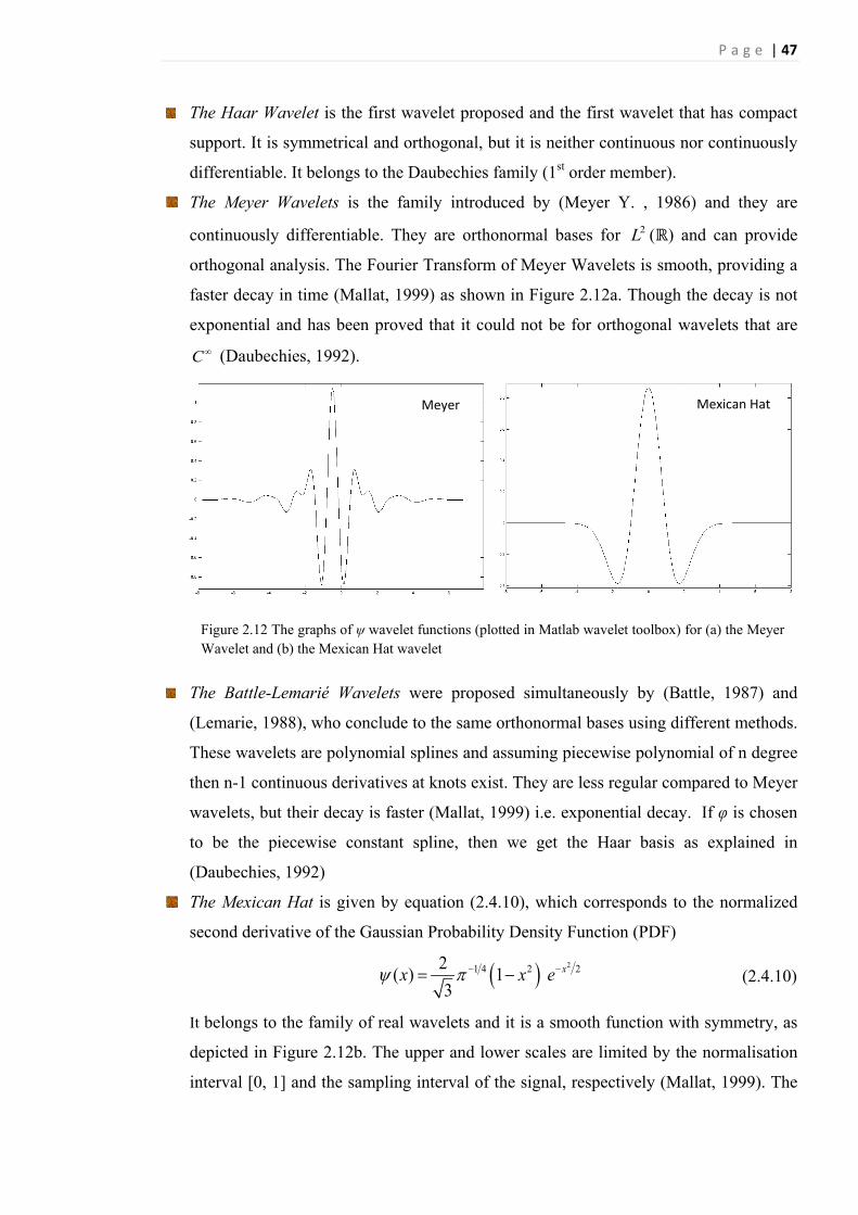


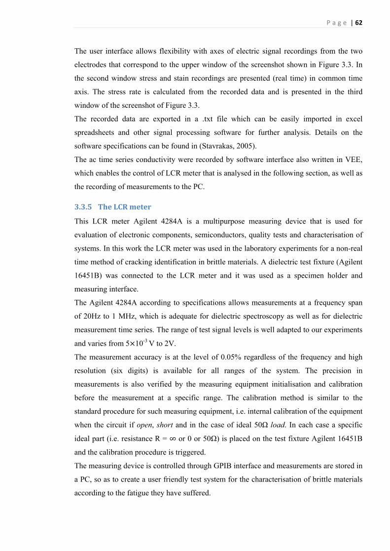


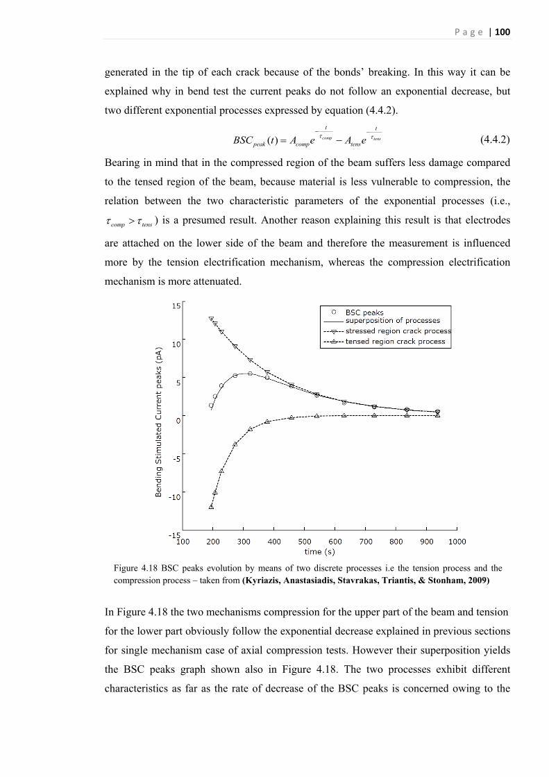


![Processing and Managing the Kepler Mission’s Treasure ... · launch pipeline design [6]. These issues stimulated significant research and devel-opment of new algorithmic approaches](https://static.documents.pub/doc/80x56/5f0949e37e708231d4261c7a/processing-and-managing-the-kepler-missionas-treasure-launch-pipeline-design.jpg)


