The development and the utilization of hyperspectralimaging devices with increased spectral, spatial, andradiometric resolution gives rise to many problemsrelated to data calibration that are difficult to solve.These problems have great significance for the re-mote sensing of the Earth because of the availabilityof new hyperspectral sensors with increased radio-metric resolution ~as much as 12–16 bits of digitizedaccuracy!. The extended dynamic range of moderndetectors can be fully employed only if the image datacan be correctly calibrated to avoid the effects of noisepatterns and other disturbances that seriously re-duce the data quality.1–3
It can easily be shown that remotely sensed imagesacquired by most kinds of sensor are generally af-fected by standard noise and by nonperiodic distur-bance patterns that show a coherent spatial andspectral structure. The amplitude of these distur-bance patterns that are superimposed upon the ob-served target may be quite large ~as much as 20–30%of the unperturbed signal! and is enhanced by thepatterns’ spatial coherence. The traditional way toremove these patterns, flat-field calibration, becomes
A. Barducci and I. Pippi [email protected]! are with the Isti-tuto di Ricerca sulle Onde Elettromagnetiche “Nello Carrara,”Consiglio Nazionale delle Ricerche, Via Panciatichi 64, Florence50127, Italy.
Received 12 April 2000; revised manuscript received 20 Novem-ber 2000.
1464 APPLIED OPTICS y Vol. 40, No. 9 y 20 March 2001
a less practical strategy as long as the digitized ac-curacy and the detector’s dynamic range increase.From a general standpoint two difficulties limit theapplication of flat-field measurements: the scarcityof laboratory sources whose output can be controlledwith high spatial and spectral accuracy ~e.g., 1 part in5000 for a 12-bit sensor! and the effects of randomnoise that may be mitigated by averaging of severalindependent measurements but then would also re-quire careful control of the source output over time.Satellite sensors can be influenced by aging that canno longer be accounted for by laboratory measure-ments but could affect the detector’s response.Moreover, some types of detector ~e.g., multiplexedscanning arrays! require continual recalibration toaccommodate the gain drift among the built-in read-out channels.4 Flat-field calibration of scanning de-vices is impossible, however, but the images of thesedevices are always influenced by disturbance pat-terns generated by the scanning system. For allthese reasons it is important to have reliable algo-rithms with which to identify and remove such co-herent patterns of disturbance.
In this paper, image restoration from some types ofnoise pattern ~mainly stripe noise! is examined. Themage-formation process that characterizes the sen-ors ~mainly imaging spectrometers and scanning de-ices! is discussed first. Some typical examples ofoherent disturbance patterns that affect remotelyensed images acquired by different kinds of sensorre then presented. This analysis permits the iden-ification of the general behavior of the disturbancesnd the design of some rejection algorithms that canetrieve the restored image of the observed target.
tfg
oohimpcsmotfn
pV
r
l
The application of the depicted algorithms to hyper-spectral images acquired by various sensors, includ-ing the Visible Infrared Scanner ~VIRS!, the AirborneThematic Mapper ~ATM!, the Thermal Infrared Mul-ispectral Scanner ~TIMS!, and the Multispectral In-rared and Visible Imaging Spectrometer ~MIVIS!,ave excellent results.
2. Theory
It has been shown5 that different kinds of noise, ~1!periodic ~both stationary and nonstationary!, ~2! co-herent ~nonperiodic!, ~3! random, and ~4! isolated, canaffect the remotely sensed images. The first type ofnoise ~which can be generated by electromagnetic in-terference! is nearly deterministic and shows a peri-dic spatial pattern whose phase and amplitude mayr may not be constant. The second kind of noiseas a partially deterministic nature and produces
rregular spatial patterns in the affected images. Inultispectral images this type of disturbance could
roduce a different pattern in each available mono-hromatic image; therefore the noise is said to bepatially and spectrally coherent. Two of the afore-entioned kinds of disturbance @types ~1! and ~2!# are
ften referred to as pattern noise, which is the mainopic of this paper. Pattern noise is distinguishedrom types ~3! and ~4!, which are defined as temporaloise.4–6
The third type is standard noise, which originatesfrom a fully stochastic process and does not show anyspatial structure or order in the affected image.Usually it is also the main limitation on the signal-to-noise ratio of the image and is therefore an impor-tant parameter that must be carefully considered fortheoretical interpretation of the data.3,7 Isolatednoise also has a stochastic nature, but it is charac-terized by the large amplitude perturbation of thesignal ~spikes! revealed in a limited number of image
ixels or lines ~which are often saturated or dark!.arious authors5–7 have discussed more fully the dis-
turbances that affect different types of digital image.
A. Coherent Noise Patterns
It can be shown that all the aforementioned types ofdisturbance often affect remotely sensed images ofthe Earth. Periodic, random, and isolated noise canbe strongly reduced by use of improved electronic andoptical components, whereas the origin of spatiallyand spectrally coherent patterns of disturbancesseems to be related to the image-formation processitself. This kind of noise characterizes most digitalimaging devices for remote sensing and other appli-cations, independently from their configurations andoperating modes. The origin of coherent noise indigital devices of two different types, whisk-broomand push-broom imaging spectrometers, is analyzedhere. The expression “imaging spectrometer” is of-ten applied to those multispectral sensors that cansample the observed spectrum without the need forany scanning mechanism of the spectrometer’s exitslit. This expression is widely used even if no trueimage is formed at the spectrometer exit slit plane.
Two widely different kinds of device, scanning de-vices and matrix-array detectors, are designated im-aging spectrometers. In contrast to scanningdevices, matrix-array detectors do not employ anyscanning mechanism with which to observe varioustarget areas. For the present study it is necessary todifferentiate between these two types of sensor.Therefore, in what follows, we refer to push-broomimaging spectrometers simply as imaging spectrom-eters ~or matrix-array sensors!; the other kinds ofemote sensors are called simply scanning devices.
B. Matrix-Array Sensors
Imaging spectrometers include matrix-array detec-tors, which can capture a full image without the useof any scanning system.5 This kind of sensor alsoincludes a spectrometer, and its general layout isdepicted schematically in Fig. 1. The detector canbe a CCD matrix array on which the spectrum of eachtarget line is imaged by the spectrometer. Thus acertain CCD line of elements corresponds to a fixedwavelength of the spectrometer’s free spectral range,so each monochromatic image is sequentially ac-quired by the same row of CCD elements located atthe corresponding wavelength. Because of thischaracteristic, the existence of CCD sensitivity clus-ters has a great effect on acquired images. As can beseen from Fig. 1, the nonuniform distribution of sen-sitivity among the elements of the matrix detectorsuperimposes a systematic pattern of noise organizedby lines upon the target image acquired by the sen-sor. Therefore, the noise pattern will have a par-tially deterministic nature and will change withwavelength because the CCD’s sensitivity generallyhas different distributions for the various rows ofelements. We refer to this disturbance as a ~spatial-y and spectrally! coherent noise pattern, which
should affect each pixel spectrum as well as the in-tensity distribution ~texture! of each monochromaticimage. Figure 1 shows the entire image-formationprocess and explains how the coherent noise pattern
Fig. 1. Layout of an imaging spectrometer that shows the originof spatially coherent patterns of noise. The pattern depends onthe wavelength ~CCD row! selected: The disturbance is thereforealso spectrally coherent.
20 March 2001 y Vol. 40, No. 9 y APPLIED OPTICS 1465
dtwS
Tnsarnsslcstmmfaca
tbagsiatihfiw~b
ssmt
1
originates in imaging spectrometer devices. Let usnote that the scheme shown in Fig. 1 is slightly sim-plified; some characteristics, which can account formore-complex scanning mechanisms inside the arraydetector, are neglected.
To clarify this phenomenon further we write therelationship among the signal g output by the matrixdetector, its sensitivity S, and the impinging radiancei. Let H~l! indicate the spectrometer’s point-spreadfunction ~PSF!; then we have
g~j, h, t! 5 @i~x, y, l! p H~l!#S~j, h! 1 g0~j, h, t!,
t 5 t~y!, h 5 h~l!, j 5 j~x!, (1)
where t is the time, ~j and h! are the coordinatesmeasured over the detector’s surface, ~x and y! arethe coordinates of an imaged ground point, and l isthe wavelength. Note that for convolution we haveintroduced the p between the spectrometer PSF’s andthe input spectrum i~x, y, l!, with the implicit as-sumption that the spectrometer has an ideal re-sponse on the x axis, so it can be represented by alinear PSF H~l! constant for all points of the spec-trometer entrance slit. When this assumption doesnot hold true, a two-dimensional PSF, e.g., a separa-ble PSF Hl~l!Hx~x!, should be included in Eq. ~1!.Term g0 on the right-hand side of Eq. ~1! is related tothe detector dark current and can therefore dependon the chosen photosensitive element ~j, h! as well ason the chosen instant t. Ideally, the horizontal~cross-track! coordinates j and x are connected by theoptical system, often by a linear relationship j~x!.Function h~l! reflects the way in which the imageformed at the spectrometer’s exit slit is sampled bythe coupled matrix–detector. Finally, t~y! is thetime–position ratio that is typical of the imaging sys-tem considered. To simplify the understanding ofEq. ~1! it is possible to cancel the parameters j, h, andt by expressing them as implicit functions of the re-maining unknowns. This will yield
g~x, y, l! 5 @i~x, y, l! p H~l!#S~x, l! 1 g0~x, y, l!, (2)
where ~x, y! can now be defined as the spatial coor-inates in the digitized image. Equation ~2! meanshat the observed signal g is related to the i p H term,hich would ideally be measured by a scaling factor~x, l! and an additive term g0. It can easily be
shown that g0 is the dark-current contribution to themeasured radiance field and contains contributionsfrom random noise and bias sources. S~x, l! is theresponse of the pixel at image column x that isdragged by the platform along the y ~or t! dimensionof the image to acquire the whole image at wave-length ~spectral channel! l. It follows that S~x, l!gives rise to a systematic pattern ~disturbance! thatis constant along the image’s vertical direction andthat could change with a change in the selected spec-tral band ~i.e., the wavelength!. This last factor isalso the mathematical expression of the spatially andspectrally coherent noise pattern introduced above.When we used the VIRS in our laboratory experi-
466 APPLIED OPTICS y Vol. 40, No. 9 y 20 March 2001
ments the S fluctuations were as large as 630% of theaverage value of the noise pattern, a result that high-lights the importance of accurate sensor calibration.The relation that occurs between S and g0 also raisesinteresting questions because both quantities are re-lated to the microscopic structure of the detector and,in part, to the electronic readout circuitry.
C. Scanning Devices
A digital scanner includes a rotating ~or oscillating!mirror or other collecting optics, which scans the tar-get surface and feeds a monochromator that illumi-nates a detector that may have one or morephotosensitive elements ~often a linear array!.Within a given scan line, many image pixels ~e.g.,1000! are sequentially acquired by the sensor withoutappreciable delay, because a delay could produceholes in the reconstructed image. The typical timedelay Tp between acquisition of two successive pixelsof the same scan line generally does not exceed 30 ms.
wo successive scan lines are instead separated by aonnegligible time delay, which is determined by thecanning frequency according to the sensor’s heightnd speed. For airborne observations of a typicalemote-sensing instrument ~i.e., the ATM! the scan-ing frequency could be as low as 12.5 Hz, corre-ponding to an acquisition delay between contiguouscan lines of 0.08 s. Digital scanners are particu-arly subject to a wide variety of disturbances thatould originate from many sources. Apart from thetandard random noise that always affects any elec-ronic device, the scanning system can suffer fromechanical vibrations ~which can affect the align-ent of optical components!, electromagnetic inter-
erence, temperature drifts, detector microphonicity,nd so on. Each of the aforementioned phenomenaan introduce noise and other disturbances into thecquired images.From a physical point of view, the appearance of
hese effects would strongly depend on a distur-ance’s frequency and coherence time scale. For ex-mple, disturbances characterized by frequenciesreater than the pixel-acquisition frequency and ahort coherence time should appear in the gatheredmages as a randomized signal that does not showny spatial structure. Instead, for lower frequencieshe disturbance could not produce any appreciablenfluence over a single image scan line because of theigh value of the pixel sampling rate. These low-requency disturbances, however, could have a signif-cant differential effect over adjacent scan lines,hich are instead acquired at a very low scan rate
;12 Hz!. We can understand this behavior bettery considering the following mathematical steps.Let s~t! be the true signal, which should be mea-
ured when one is observing the target with an idealensor that is not affected by any disturbance. Let~t! represent a null-mean signal modulation ~mul-
iplicative disturbance! introduced by the aforemen-
ldt
s
paaeaf
c
wts
tm
mssIbstpdoea
aapwapacib
wsE
t
gs
ncatup
tioned phenomena; then the gathered pixel value g~t!can be represented by the following law:
g~t! 5 *2`
1`
p~x, y, t 2 t!@1 1 m~t!#s~t!dt,
t 5 t~x, y!, (3)
where the pupil function p~x, y, t 2 t!, which definesintegration time tp ~for example, 3 ms! for the pixelocated at point x, y of the image, has been intro-uced. It should be noted that pixel integrationime tp has to be far below time delay Tp between
adjacent pixels. In fact, time step Tp, which sepa-rates the acquisition of two consecutive picture el-ements, is chosen according to the detector’sinstantaneous field of view ~IFOV! to ensure correctampling:
2pfl Tp < IFOVya. (4)
Here fl is the line frequency, and the oversamplingfactor ~a . 1! can accommodate the nonideal low-
ass filter that performs the image reconstructionnd guarantees that the measured image is notliased. It is worth noting that imaging spectrom-ters do not comply with this quality requirementnd that the images that they supply should there-ore be aliased.
Note that s~t! is assumed to be a band-limited sig-nal. In fact, the bandwidth of s~t! is limited by thespatial integration performed by the photosensitiveelement that collects the impinging radiance. Thetime-equivalent duration of this spatial integration,determined by the IFOV and the line frequency of thesensor, is IFOVy2pfl and exceeds sampling step Tp byoversampling factor a. As a consequence, the max-imum frequency contained in s~t! is roughly equiva-lent to 2pflyIFOV; thus its sampling meets theonditions of the popular Shannon theorem.
Modulation m~t!, however, can have an evenider spectrum but one that would be limited by the
ime integration performed during the pixel acqui-ition. Unfortunately pixel integration time tp is
appreciably shorter than pixel sampling step Tp, sohe maximum frequency for the spectrum of signal~t! is ;1ytp, a value that is greater than the sam-
pling frequency. In other words, sampled signalg~t! will contain contributions from disturbance
~t! that are aliased. In this context aliasing of aampled random signal is remarkable not for recon-truction purposes but for energy considerations.t is well known that aliasing of noise is importantecause it folds the wider spectrum of noise in thepectral band of the interpolated signal numerousimes. The final effect is that the noise spectralower is enhanced with respect to the power of theeterministic signal, in our case the natural texturef the observed scene. This property could alsoxplain why this kind of noise is generally found incquired images.The second term of Eq. ~3! is the typical time-
position dependence that characterizes the scan-ning system used. Pupil p~x, y, t 2 t! is a stepfunction that is null for all the t 2 t values outsideperiod tp, centered on t~x, y!. Function m~t!, here-
fter called disturbance modulation, can be deviseds an ordinary, null-mean, stationary stochasticrocess. For the sake of simplicity we assume thate have a homogeneous target whose texture s~t! isslowly varying ~or constant! function of time t @i.e.,osition ~x, y!# that does not show appreciable vari-tion within the short integration time of the pixelonsidered. Modulation m~t! can be rewritten asts Fourier spectrum M~ f !, in which case Eq. ~3!ecomes
g~t! 5 s~t! *2`
1`
p~x, y, t 2 t!
3 F1 1 * M~ f !exp~2pift!dfGdt, (5)
here f is the time frequency of the disturbancepectrum. As can be shown, the right-hand side ofq. ~5! is easily integrated term by term and gives
g~t! 5 s~t!Ftp 1 * M~ f !exp~2pift!sin~pftp!
pfdfG . (6)
Note that the integral on the right-hand side of Eq.~6! can also be recognized as the diffraction pattern ofhe harmonic on the pupil-function aperture tp. By
imposing in Eq. ~3! a different assumption of additivedisturbance m, we can obtain nearly the same resultas in Eq. ~6!. To investigate the appearance of thedisturbance in the acquired image, we compute thedifference in signal between adjacent pixels ~imageradient! of the same ~horizontal component! and ofuccessive ~vertical component! scan lines:
Dx g~t! > s~t! * M~ f !exp~2pift!@exp~2pifTp! 2 1#
3sin~pftp!
pfdf,
Dy g~t! > s~t! * M~ f !exp~2pift!@exp~2pfTl! 2 1#
3sin~pftp!
pfdf. (7)
Here the scan-line acquisition period Tl has been in-troduced, and target texture s~t! has been considered
early constant for adjacent image pixels ~e.g., weonsider the effects of disturbances on the images ofhomogeneous target!. As shown in relations ~7!,
he effect of a single harmonic component of the mod-lation, as a result of the acting disturbances, de-ends strongly on the component’s frequency:
20 March 2001 y Vol. 40, No. 9 y APPLIED OPTICS 1467
an
t
ciirt
s
ardittdwsm
oi
etas
daAs
wstsab
1
For modulation frequencies f far above pixel-cquisition frequency fp ~ fp 5 1yTp!, we have a non-egligible difference Dxg between adjacent pixels of
the same scan line. This quantity Dxg can changeunpredictably with respect to horizontal coordinatex. In fact, time difference Tp, corresponding to adisplacement of only one pixel along the image scanline, represents a delay of several periods at mod-ulation frequency f. When the time has elapsed,he phase of the disturbance can change. As Tl is
greater than Tp, pixel difference Dyg between suc-essive scan lines will have exactly the same behav-or as Dxg; therefore the effect of signal modulationnduced by such high-frequency components is aandomized disturbance superimposed upon thearget texture.
When modulation frequency f is far below fp butstill is comparable with or greater than line fre-quency fl ~ fl 5 1yTl!, we no longer have any horizon-tal difference Dxg, whereas a strong verticaldifference Dyg can still be found. This vertical dif-ference will change slightly along the same scan line,as the pixel’s frequency is much greater than that ofthe modulation. This means that the modulation’scomponents whose frequency falls within this fre-quency range ~ fl–fp! should appear in the acquiredimage as a spatially coherent noise pattern, orga-nized into horizontal lines ~e.g., the stripe noise!. Fi-nally, even if line-scanning frequency fl is far abovethe considered frequency of the modulation spec-trum, the related disturbance does not affect the im-age, except for a slow variation of the image’s meanbrightness.
For typical remote-sensing instruments, the twofundamental frequencies of the scanning systemhave the following magnitudes: fl ; 10 and fp ; 105
Hz. Considering these values and the analysis asexecuted, it is possible to outline the effects on theimage of the various disturbance sources. Mechan-ical vibrations that affect the performance of the op-tical system should operate only at lower frequencies.Their cutoff frequencies can be estimated as 103–104
Hz. Therefore their effect on the acquired imagesshould be to produce a coherent noise pattern orga-nized by image scan lines. Electromagnetic detectorperturbations can instead have a wider frequencyspectrum. Radio- and higher-frequency wavesshould generally decrease the effective signal-to-noise ratio of the sensor, as their frequency is farabove pixel frequency fp. At electromagnetic fre-quencies equal or comparable with fp the related im-age effect could even be a periodic pattern of noise, atleast if the disturbance source is time coherent ~theource phase is constant for periods greater than Tl!.
468 APPLIED OPTICS y Vol. 40, No. 9 y 20 March 2001
3. Numerical Simulations
To verify the predictions of the simple analysis shownin the previous sections, we carried out simulations ofthe signal described by Eq. ~6!. Because of the sim-ple form of Eq. ~2! the result of the analysis has notbeen numerically computed.
We executed simulations by considering a uni-form target @i.e., a constant texture s~t!# dimmed by
disturbance m~t! with a selectable spectrum ~Fou-ier transform! and coherence time. Two kinds ofisturbance, monochromatic harmonics and Gauss-an envelopes, were tried. In the second case bothhe central frequency and the passband width wereunable. We completed disturbance m~t! by intro-ucing a characteristic coherence time scale t0,hich plays a fundamental role in determining the
patial structure of the disturbance. This goal wasathematically achieved by addition of a phase w to
the principal argument t of modulation m~t!. Inur simulations, phase w is constant for a long timenterval tc when it is randomly changed. The cur-
rent value of coherence time length tc is randomlyestimated each time that phase w changes. Theestimate of parameter tc was constrained to have amean value equal to the constant value ^tc& 5 t0.Time constants Tp and Tl that describe the simu-lated detector were fixed at values of 1025 and 8 31022 s, respectively, a choice that closely accountsfor the use of many airborne scanning sensors ~forxample, the ATM and the TIMS!. Each simula-ion run produced a synthetic image that shows theppearance of the corresponding disturbance in thepatial domain.Figure 2 shows the simulation of a monochromatic
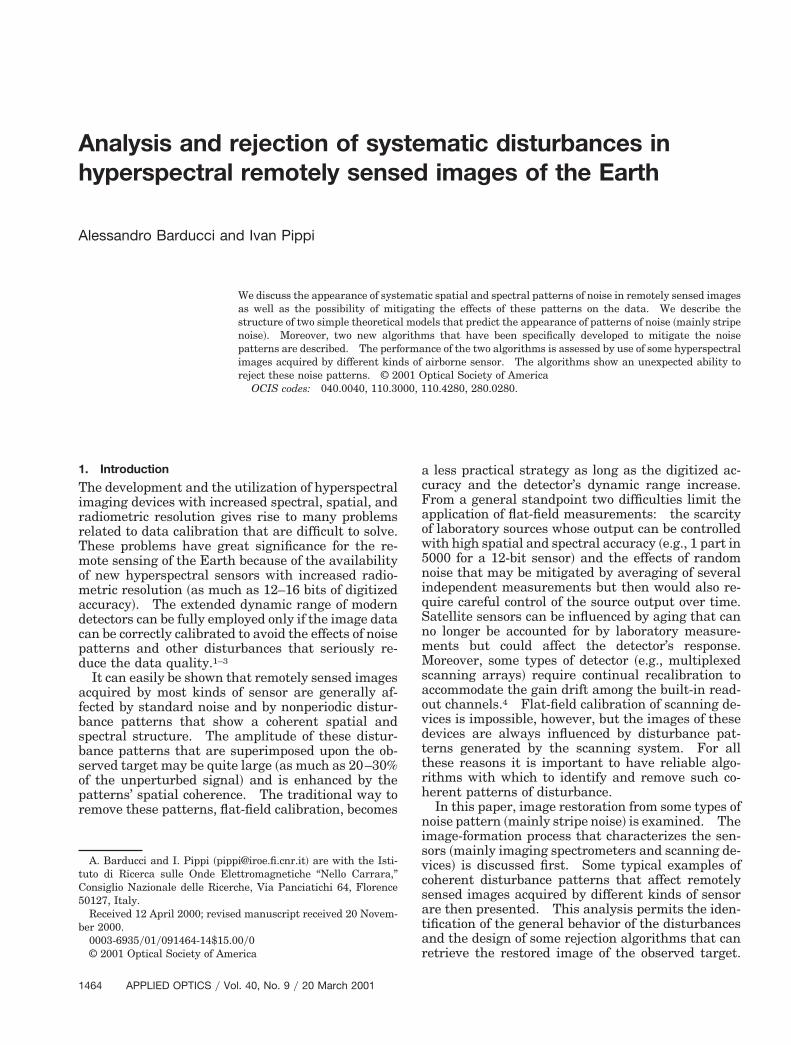
isturbance that has a frequency of 679 kHz and anverage time scale of coherence equal to 30 periods.s expected, the disturbance resembles a randomignal ~salt–pepper noise!, which affects mainly the
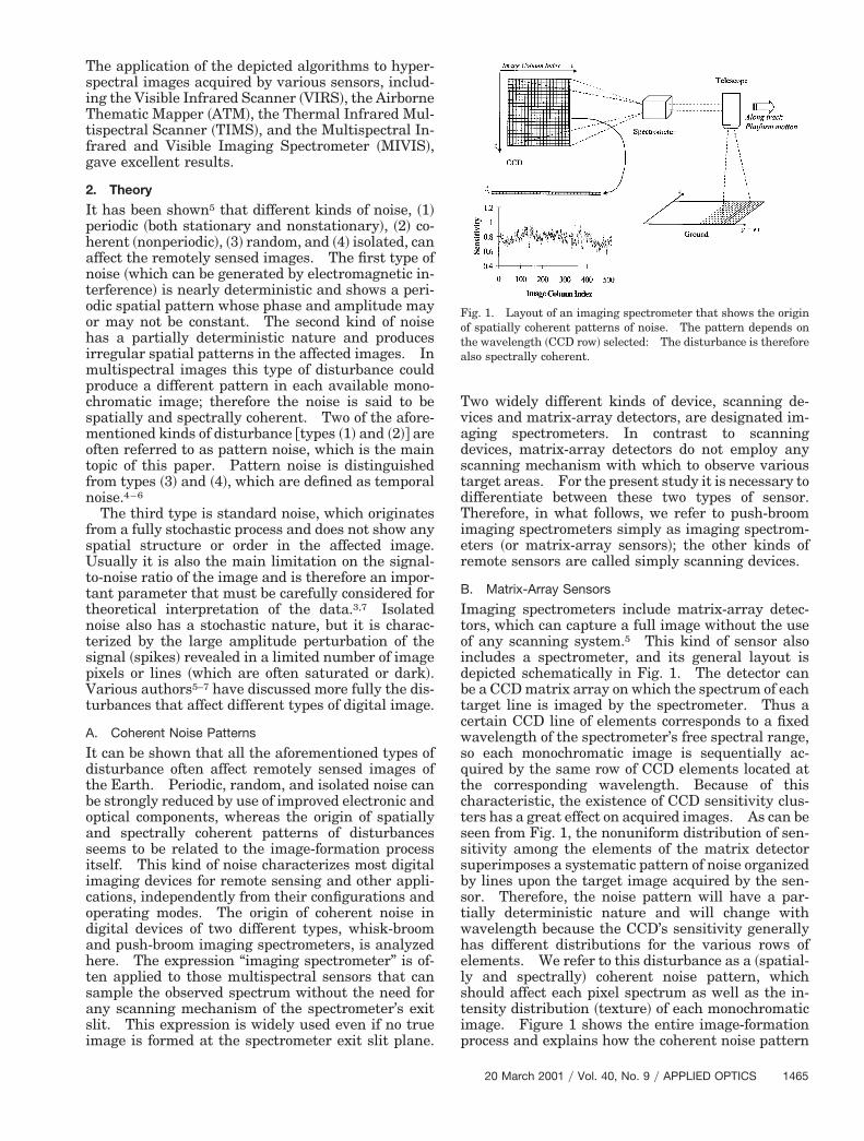
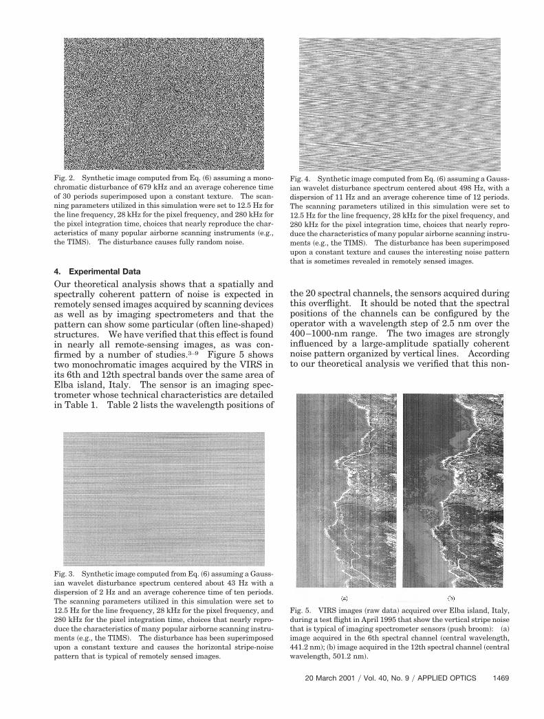
image’s signal-to-noise ratio. Simulations of distur-bances with Gaussian envelopes are shown in Figs. 3and 4. The disturbance shown in Fig. 3 is related toa low central frequency ~43-Hz! modulation with 2-HzFWHM and a coherence time scale of 10 periods. Ascan be seen, this disturbance produces a horizontalline–shaped pattern that is found in almost all im-ages gathered by scanning devices. A disturbance ofhigher central frequency ~498 Hz! is shown in Fig. 4,
here a nonperiodic pattern of alternate dark–brightlant areas is shown. Finally, our simulations showhat when one considers an endless coherence timecale ~to .. Tl! a periodic pattern is always obtained,t least for monochromatic or narrow-band distur-ances.
Dx g Þ 0, Dy g Þ 0 for fTl $ fTp .. 1 ~randomized disturbance!,Dx g 5 0, Dy g Þ 0 for fTl $ 1 .. fTp ~spatially coherent pattern!,Dx g 5 0, Dy g 5 0 for 1 .. fTl $ fTp ~image brightness scaling!,
(8)
sifi
dt
4. Experimental Data
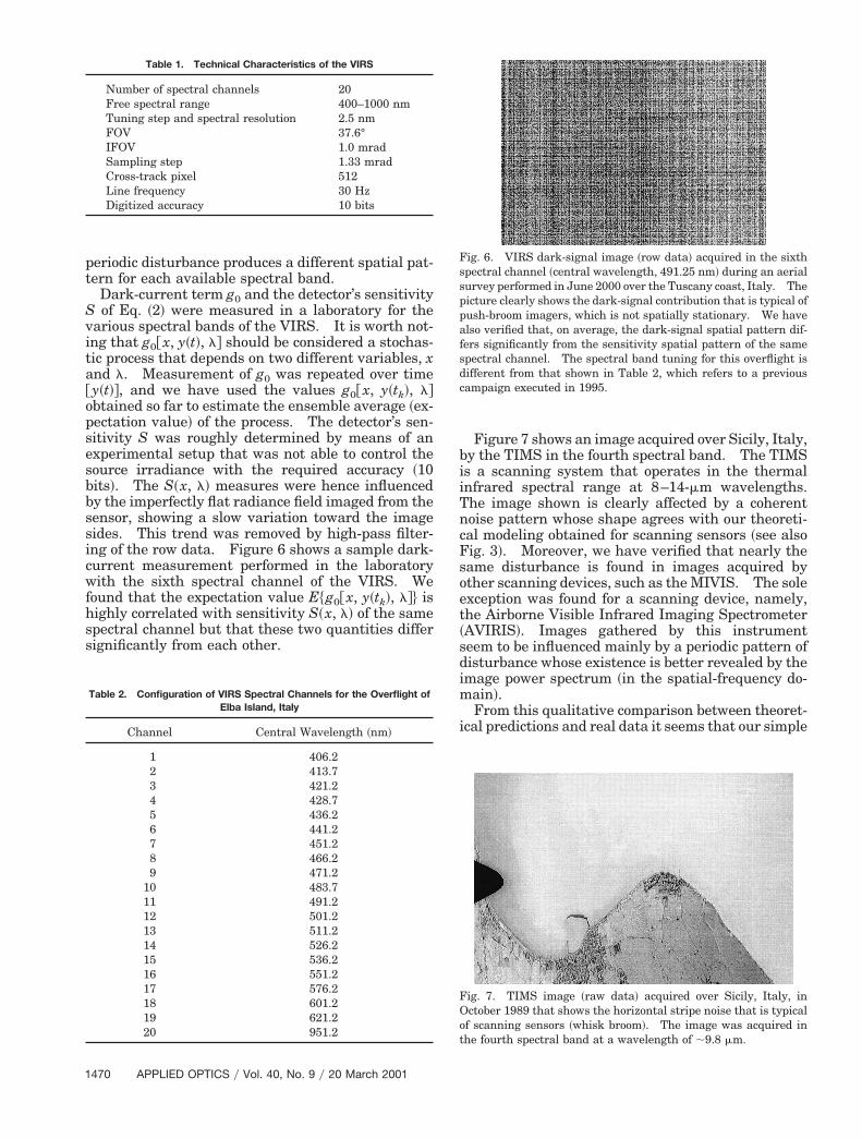
Our theoretical analysis shows that a spatially andspectrally coherent pattern of noise is expected inremotely sensed images acquired by scanning devicesas well as by imaging spectrometers and that thepattern can show some particular ~often line-shaped!tructures. We have verified that this effect is foundn nearly all remote-sensing images, as was con-rmed by a number of studies.3–9 Figure 5 shows
two monochromatic images acquired by the VIRS inits 6th and 12th spectral bands over the same area ofElba island, Italy. The sensor is an imaging spec-trometer whose technical characteristics are detailedin Table 1. Table 2 lists the wavelength positions of
Fig. 2. Synthetic image computed from Eq. ~6! assuming a mono-chromatic disturbance of 679 kHz and an average coherence timeof 30 periods superimposed upon a constant texture. The scan-ning parameters utilized in this simulation were set to 12.5 Hz forthe line frequency, 28 kHz for the pixel frequency, and 280 kHz forthe pixel integration time, choices that nearly reproduce the char-acteristics of many popular airborne scanning instruments ~e.g.,the TIMS!. The disturbance causes fully random noise.
Fig. 3. Synthetic image computed from Eq. ~6! assuming a Gauss-ian wavelet disturbance spectrum centered about 43 Hz with adispersion of 2 Hz and an average coherence time of ten periods.The scanning parameters utilized in this simulation were set to12.5 Hz for the line frequency, 28 kHz for the pixel frequency, and280 kHz for the pixel integration time, choices that nearly repro-duce the characteristics of many popular airborne scanning instru-ments ~e.g., the TIMS!. The disturbance has been superimposedupon a constant texture and causes the horizontal stripe-noisepattern that is typical of remotely sensed images.
the 20 spectral channels, the sensors acquired duringthis overflight. It should be noted that the spectralpositions of the channels can be configured by theoperator with a wavelength step of 2.5 nm over the400–1000-nm range. The two images are stronglyinfluenced by a large-amplitude spatially coherentnoise pattern organized by vertical lines. Accordingto our theoretical analysis we verified that this non-
Fig. 4. Synthetic image computed from Eq. ~6! assuming a Gauss-ian wavelet disturbance spectrum centered about 498 Hz, with adispersion of 11 Hz and an average coherence time of 12 periods.The scanning parameters utilized in this simulation were set to12.5 Hz for the line frequency, 28 kHz for the pixel frequency, and280 kHz for the pixel integration time, choices that nearly repro-duce the characteristics of many popular airborne scanning instru-ments ~e.g., the TIMS!. The disturbance has been superimposedupon a constant texture and causes the interesting noise patternthat is sometimes revealed in remotely sensed images.
Fig. 5. VIRS images ~raw data! acquired over Elba island, Italy,uring a test flight in April 1995 that show the vertical stripe noisehat is typical of imaging spectrometer sensors ~push broom!: ~a!
image acquired in the 6th spectral channel ~central wavelength,441.2 nm!; ~b! image acquired in the 12th spectral channel ~centralwavelength, 501.2 nm!.
20 March 2001 y Vol. 40, No. 9 y APPLIED OPTICS 1469
vi
Fsoet~sdim
i
Table 1. Technical Characteristics of the VIRS
1
periodic disturbance produces a different spatial pat-tern for each available spectral band.
Dark-current term g0 and the detector’s sensitivityS of Eq. ~2! were measured in a laboratory for thearious spectral bands of the VIRS. It is worth not-ng that g0@x, y~t!, l# should be considered a stochas-
tic process that depends on two different variables, xand l. Measurement of g0 was repeated over time@y~t!#, and we have used the values g0@x, y~tk!, l#obtained so far to estimate the ensemble average ~ex-pectation value! of the process. The detector’s sen-sitivity S was roughly determined by means of anexperimental setup that was not able to control thesource irradiance with the required accuracy ~10bits!. The S~x, l! measures were hence influencedby the imperfectly flat radiance field imaged from thesensor, showing a slow variation toward the imagesides. This trend was removed by high-pass filter-ing of the row data. Figure 6 shows a sample dark-current measurement performed in the laboratorywith the sixth spectral channel of the VIRS. Wefound that the expectation value E$g0@x, y~tk!, l#% ishighly correlated with sensitivity S~x, l! of the samespectral channel but that these two quantities differsignificantly from each other.
Number of spectral channels 20Free spectral range 400–1000 nmTuning step and spectral resolution 2.5 nmFOV 37.6°IFOV 1.0 mradSampling step 1.33 mradCross-track pixel 512Line frequency 30 HzDigitized accuracy 10 bits
Table 2. Configuration of VIRS Spectral Channels for the Overflight ofElba Island, Italy
470 APPLIED OPTICS y Vol. 40, No. 9 y 20 March 2001
Figure 7 shows an image acquired over Sicily, Italy,by the TIMS in the fourth spectral band. The TIMSis a scanning system that operates in the thermalinfrared spectral range at 8–14-mm wavelengths.The image shown is clearly affected by a coherentnoise pattern whose shape agrees with our theoreti-cal modeling obtained for scanning sensors ~see also
ig. 3!. Moreover, we have verified that nearly theame disturbance is found in images acquired byther scanning devices, such as the MIVIS. The solexception was found for a scanning device, namely,he Airborne Visible Infrared Imaging SpectrometerAVIRIS!. Images gathered by this instrumenteem to be influenced mainly by a periodic pattern ofisturbance whose existence is better revealed by themage power spectrum ~in the spatial-frequency do-
ain!.From this qualitative comparison between theoret-
cal predictions and real data it seems that our simple
Fig. 6. VIRS dark-signal image ~row data! acquired in the sixthspectral channel ~central wavelength, 491.25 nm! during an aerialsurvey performed in June 2000 over the Tuscany coast, Italy. Thepicture clearly shows the dark-signal contribution that is typical ofpush-broom imagers, which is not spatially stationary. We havealso verified that, on average, the dark-signal spatial pattern dif-fers significantly from the sensitivity spatial pattern of the samespectral channel. The spectral band tuning for this overflight isdifferent from that shown in Table 2, which refers to a previouscampaign executed in 1995.
Fig. 7. TIMS image ~raw data! acquired over Sicily, Italy, inOctober 1989 that shows the horizontal stripe noise that is typicalof scanning sensors ~whisk broom!. The image was acquired inthe fourth spectral band at a wavelength of ;9.8 mm.
t
models ~for both scanning sensors and imaging spec-rometers! are in good agreement with experimental
data. Deeper insights can be obtained from compar-ison of our simulations with the results reported byWatson,8 who also investigated the problem of image
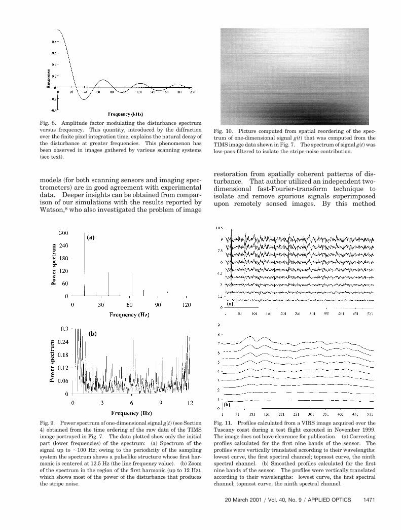
Fig. 8. Amplitude factor modulating the disturbance spectrumversus frequency. This quantity, introduced by the diffractionover the finite pixel integration time, explains the natural decay ofthe disturbance at greater frequencies. This phenomenon hasbeen observed in images gathered by various scanning systems~see text!.
Fig. 9. Power spectrum of one-dimensional signal g~t! ~see Section4! obtained from the time ordering of the raw data of the TIMSimage portrayed in Fig. 7. The data plotted show only the initialpart ~lower frequencies! of the spectrum: ~a! Spectrum of thesignal up to ;100 Hz; owing to the periodicity of the samplingsystem the spectrum shows a pulselike structure whose first har-monic is centered at 12.5 Hz ~the line frequency value!. ~b! Zoomof the spectrum in the region of the first harmonic ~up to 12 Hz!,which shows most of the power of the disturbance that producesthe stripe noise.
restoration from spatially coherent patterns of dis-turbance. That author utilized an independent two-dimensional fast-Fourier-transform technique toisolate and remove spurious signals superimposedupon remotely sensed images. By this method
Fig. 10. Picture computed from spatial reordering of the spec-trum of one-dimensional signal g~t! that was computed from theTIMS image data shown in Fig. 7. The spectrum of signal g~t! waslow-pass filtered to isolate the stripe-noise contribution.
Fig. 11. Profiles calculated from a VIRS image acquired over theTuscany coast during a test flight executed in November 1999.The image does not have clearance for publication. ~a! Correctingprofiles calculated for the first nine bands of the sensor. Theprofiles were vertically translated according to their wavelengths:lowest curve, the first spectral channel; topmost curve, the ninthspectral channel. ~b! Smoothed profiles calculated for the firstnine bands of the sensor. The profiles were vertically translatedaccording to their wavelengths: lowest curve, the first spectralchannel; topmost curve, the ninth spectral channel.
20 March 2001 y Vol. 40, No. 9 y APPLIED OPTICS 1471
pvwf
fi
sbptb
1
Watson8 was able to find a series of different andindependent disturbances of decreasing amplitude~see Figs. 6 and 7 of Ref. 8!. Generally, the firstdisturbance of his series is the same as our simulateddisturbance shown in Fig. 3, for a modulation centralfrequency of 43 Hz. It is worth noting that the nexthigher frequency disturbance that we found ~shownin Fig. 4! is nearly the same as the second patternrecognized by Watson8 and shown in his Fig. 7E. Inaddition, for a narrow-band disturbance of high fre-quency, our simulations produced spatial patternssimilar to those shown in Figs. 7C and 7D of Watson.8The circumstances described above validate the re-sults predicted by our simple model of scanning sys-tems. We also point out that at a fixed energy ofmodulation m~t! the disturbance amplitude revealedin our simulated images decreases with increasingmodulation frequency, according to the sinc factorheld in Eq. ~6! and produced by the finite value of the
ixel integration time. This slow amplitude decayersus frequency is plotted in Fig. 8, the data of whiche computed numerically by adopting the same data
or Tp and Tl as were utilized in the other simula-tions. These data are valid for the sensor TIMS, asis the case of the analysis by Watson.8 This behav-ior accounted for by our model can therefore success-fully explain the decreasing amplitude measured by
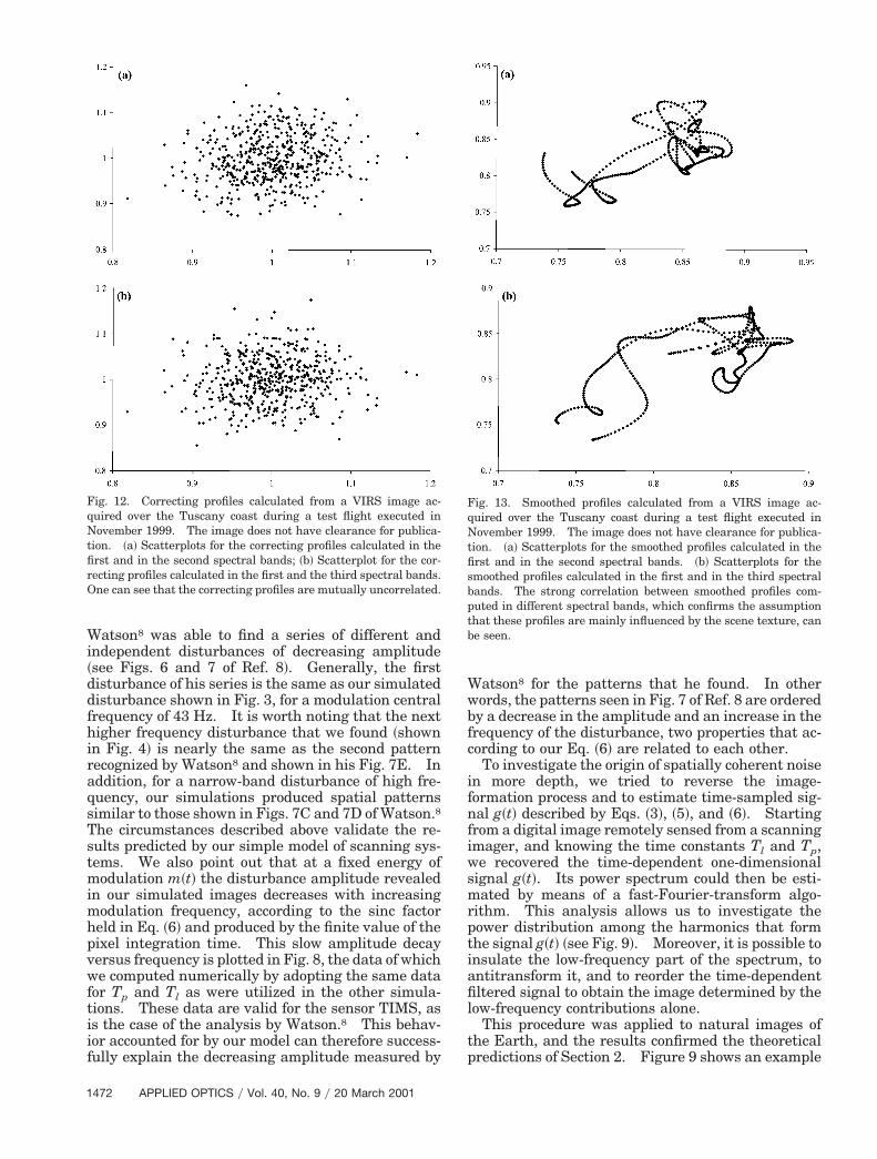
Fig. 12. Correcting profiles calculated from a VIRS image ac-quired over the Tuscany coast during a test flight executed inNovember 1999. The image does not have clearance for publica-tion. ~a! Scatterplots for the correcting profiles calculated in thefirst and in the second spectral bands; ~b! Scatterplot for the cor-recting profiles calculated in the first and the third spectral bands.One can see that the correcting profiles are mutually uncorrelated.
472 APPLIED OPTICS y Vol. 40, No. 9 y 20 March 2001
Watson8 for the patterns that he found. In otherwords, the patterns seen in Fig. 7 of Ref. 8 are orderedby a decrease in the amplitude and an increase in thefrequency of the disturbance, two properties that ac-cording to our Eq. ~6! are related to each other.
To investigate the origin of spatially coherent noisein more depth, we tried to reverse the image-formation process and to estimate time-sampled sig-nal g~t! described by Eqs. ~3!, ~5!, and ~6!. Startingrom a digital image remotely sensed from a scanningmager, and knowing the time constants Tl and Tp,
we recovered the time-dependent one-dimensionalsignal g~t!. Its power spectrum could then be esti-mated by means of a fast-Fourier-transform algo-rithm. This analysis allows us to investigate thepower distribution among the harmonics that formthe signal g~t! ~see Fig. 9!. Moreover, it is possible toinsulate the low-frequency part of the spectrum, toantitransform it, and to reorder the time-dependentfiltered signal to obtain the image determined by thelow-frequency contributions alone.
This procedure was applied to natural images ofthe Earth, and the results confirmed the theoreticalpredictions of Section 2. Figure 9 shows an example
Fig. 13. Smoothed profiles calculated from a VIRS image ac-quired over the Tuscany coast during a test flight executed inNovember 1999. The image does not have clearance for publica-tion. ~a! Scatterplots for the smoothed profiles calculated in thefirst and in the second spectral bands. ~b! Scatterplots for themoothed profiles calculated in the first and in the third spectralands. The strong correlation between smoothed profiles com-uted in different spectral bands, which confirms the assumptionhat these profiles are mainly influenced by the scene texture, cane seen.
iTfdpo
ttn
6
of a one-dimensional power spectrum calculated froma TIMS image acquired over Sicily, Italy, in 1988.Note that the spectrum has a typical spikelike ap-pearance ~recalling that of television signals!, whichs related to the periodicity of the sampling process.he same figure also shows an expansion of the low-
requency part of the spectrum that contributes to theisturbance. Finally, Fig. 10 shows the image com-uted after application of the low-pass filter to theriginal one-dimensional signal g~t!. The cutoff fre-
quency used in this circumstance was empirically setat 50 Hz, a value that is consistent with our theory.This result is impressive when it is compared withthat for the stripe noise that affects the original im-age data.
This kind of analysis was repeated for images gath-ered from many different aerial and satellite-basedsensors ~e.g., ATM and MIVIS!. We have not foundcircumstances in which this procedure gave incorrectoutcomes: It was always able to retrieve the noisypart of the original image data.
5. Rejection of Coherent Noise Patterns
It is evident that, because of its partially determin-istic nature, any spatially coherent noise patterncould theoretically be mitigated by an appropriatecorrecting procedure without appreciable loss ofspatial and spectral resolution. Therefore we havedeveloped two new algorithms devoted to the res-toration of images acquired by linear scanners andmatrix arrays. The two algorithms independentlyprocess each available spectral band, and theirmost important feature is related to the circum-stance that they do not affect the radiometric cali-bration of data, whose physical meaning remainsunchanged.
Fig. 14. Pixel sensitivity ~solid curve! and correcting profile ~as-erisks and dashed curve! relative to the pixel’s column index forhe sixth spectral channel of the VIRS ~central wavelength, 491.25m!. The pixel sensitivity was measured in the laboratory ~dur-
ing May 2000! with a white standard reflector ~Spectralon plate!and two commercial-grade light sources. The imaged field wasnot flat and showed a noticeable decrease toward the image sides.This slow trend was eliminated from the image data by high-passspatial filtering. The correcting profile was retrieved from thealgorithm discussed in Subsection 5.A. The ability of the algo-rithm to predict the value of the pixel sensitivity is impressive.The spectral band tuning for this measurement is different fromthat in Table 2, which refers to an overflight executed in 1995.
A. Push-Broom Imaging Spectrometers
The algorithm devoted to processing the data gath-ered by imaging spectrometers can strongly reducethe need for any flat-field calibration of the sensor,and owing to its simple structure it also is suitable forreal-time implementation.
The algorithm utilizes a subset p of the imageHough transform, chosen according to the spatialstructure of the considered noise pattern. For im-aging spectrometers this subset is defined by all theintegrals computed over image columns that producean image profile that corresponds to the average im-age horizontal line.
Let g be the raw, or the radiometrically calibrated,image gathered by a push-broom device, in which xand y are the coordinates of a generic pixel and lindicates the wavelength ~of the spectral band!.Profile p is defined by
p~x, l! 5 * g~x, y, l!dy. (9)
Profile p, which is the average image row, obviouslycontains much information on the spatial structure ofthe disturbance pattern, and, because of averaging, itis scarcely influenced by any additive random noise.Profile p also depends on the wavelength because thevalue of the integral in Eq. ~9! is different for thevarious spectral channels.
As long as a textureless image is considered, profile
Fig. 15. VIRS image ~processed data! acquired over Elba island,Italy, during a test flight in 1995. The pictures were processed bythe algorithm described here to mitigate the effects of the verticalstripe noise that is characteristic of imaging spectrometer sensors~push broom!. The weighting function half-width utilized for thisexample was set to 11 pixels: ~a! Corrected image acquired in theth spectral channel ~central wavelength, 441.2 nm!. ~b! Cor-
rected image acquired in the 12th spectral channel ~central wave-length, 501.2 nm!.
20 March 2001 y Vol. 40, No. 9 y APPLIED OPTICS 1473
sWb
gtra
1
p should reflect only the disturbance pattern. Whena real ~natural! image is considered, its texturehould have some influence on the profile obtained.e assume that, whereas the contributions of distur-
ances suddenly change with position x, those thatoriginate from the texture of the observed sceneslowly vary with x. If the analysis is executed in thespatial-frequency domain by a Fourier transform ofthe profile, we can formulate our hypothesis by stat-ing that a cutoff frequency fc should exist thatroughly splits contributions that are due to scenetexture from those that originate from the noise pat-tern. This means that for spatial frequency freater than fc the value of the profile transform is
due exclusively to the noise pattern. As long as thissupposition holds, the shape of the noise pattern canbe retrieved exactly by application of a simple high-pass frequency filter to computed profile p. Thephysical likelihood that this assumption is true canbe visually inferred from the characteristics of theraw images gathered by the sensor and shown in Fig.5.
To extract the higher-spatial-frequency compo-nents of profile p, we designed a two-stage filtering
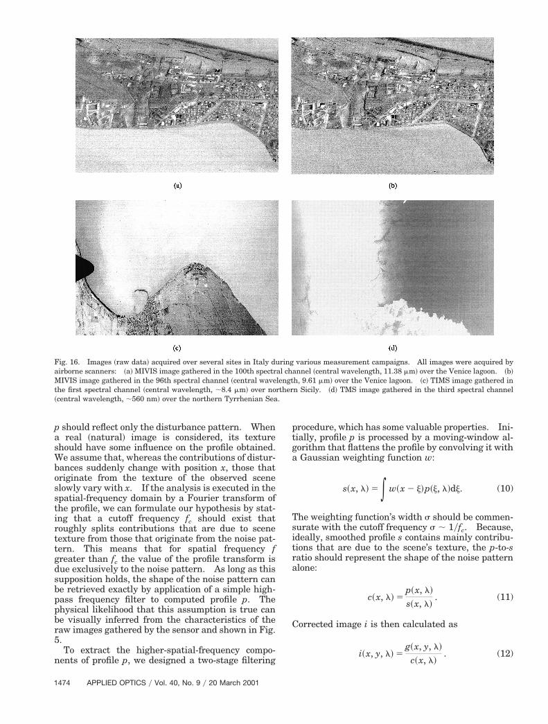
Fig. 16. Images ~raw data! acquired over several sites in Italy duairborne scanners: ~a! MIVIS image gathered in the 100th spectrMIVIS image gathered in the 96th spectral channel ~central wavethe first spectral channel ~central wavelength, ;8.4 mm! over no~central wavelength, ;560 nm! over the northern Tyrrhenian Sea
474 APPLIED OPTICS y Vol. 40, No. 9 y 20 March 2001
procedure, which has some valuable properties. Ini-tially, profile p is processed by a moving-window al-gorithm that flattens the profile by convolving it witha Gaussian weighting function w:
s~x, l! 5 * w~x 2 j!p~j, l!dj. (10)
The weighting function’s width s should be commen-surate with the cutoff frequency s ; 1yfc. Because,ideally, smoothed profile s contains mainly contribu-ions that are due to the scene’s texture, the p-to-satio should represent the shape of the noise patternlone:
c~x, l! 5p~x, l!
s~x, l!. (11)
Corrected image i is then calculated as
i~x, y, l! 5g~x, y, l!
c~x, l!. (12)
various measurement campaigns. All images were acquired byannel ~central wavelength, 11.38 mm! over the Venice lagoon. ~b!h, 9.61 mm! over the Venice lagoon. ~c! TIMS image gathered inn Sicily. ~d! TMS image gathered in the third spectral channel
ringal chlengtrther.
b
Use of a simple ratio to extract the restored imageis theoretically motivated by the circumstance thatthe removed pattern is always introduced by a scalefactor, as can be seen from Eq. ~2!.
It should be noted that the value of newly definedprofile c oscillates about the value 1. This propertygives corrected image i two important characteristics:i has on average the same intensity distribution asraw image g has, and images i and g have the samepixel spectra in any homogeneous scene region.From a practical point of view this means that thewhole correction procedure is suitable for processingradiometric calibrated data without affecting theirphysical units of measure. The algorithm guaran-tees that the image data are manipulated by main-taining, on average, the same unitary scaling factorsin all the available spectral bands. Let us note thatthe procedure outlined should also be able to restorethe images gathered by multiplexed scanning arraydetectors, a circumstance not entirely considered inthe theoretical analysis of Section 2.
The basic assumption of our model ~that textureand disturbance lie in different spatial-frequencyranges and therefore can be reliably separated by a
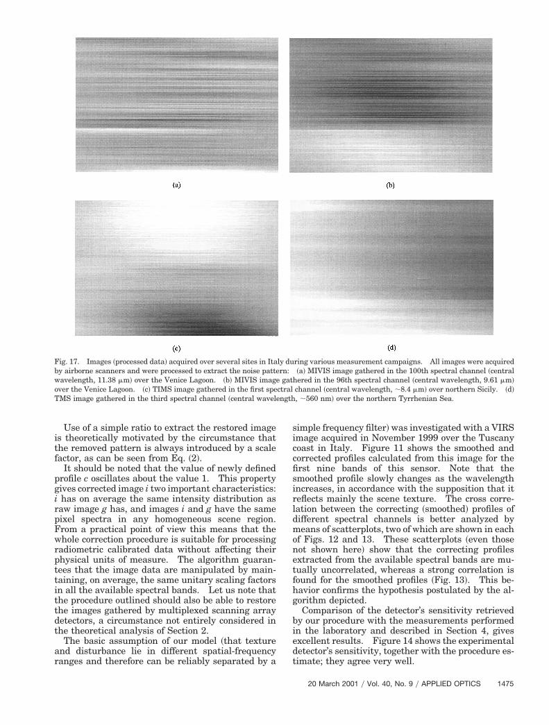
Fig. 17. Images ~processed data! acquired over several sites in Itay airborne scanners and were processed to extract the noise patte
wavelength, 11.38 mm! over the Venice Lagoon. ~b! MIVIS imagover the Venice Lagoon. ~c! TIMS image gathered in the first speTMS image gathered in the third spectral channel ~central wavel
simple frequency filter! was investigated with a VIRSimage acquired in November 1999 over the Tuscanycoast in Italy. Figure 11 shows the smoothed andcorrected profiles calculated from this image for thefirst nine bands of this sensor. Note that thesmoothed profile slowly changes as the wavelengthincreases, in accordance with the supposition that itreflects mainly the scene texture. The cross corre-lation between the correcting ~smoothed! profiles ofdifferent spectral channels is better analyzed bymeans of scatterplots, two of which are shown in eachof Figs. 12 and 13. These scatterplots ~even thosenot shown here! show that the correcting profilesextracted from the available spectral bands are mu-tually uncorrelated, whereas a strong correlation isfound for the smoothed profiles ~Fig. 13!. This be-havior confirms the hypothesis postulated by the al-gorithm depicted.
Comparison of the detector’s sensitivity retrievedby our procedure with the measurements performedin the laboratory and described in Section 4, givesexcellent results. Figure 14 shows the experimentaldetector’s sensitivity, together with the procedure es-timate; they agree very well.
ring various measurement campaigns. All images were acquired~a! MIVIS image gathered in the 100th spectral channel ~central
hered in the 96th spectral channel ~central wavelength, 9.61 mm!channel ~central wavelength, ;8.4 mm! over northern Sicily. ~d!, ;560 nm! over the northern Tyrrhenian Sea.
ly durn:
e gatctralength
20 March 2001 y Vol. 40, No. 9 y APPLIED OPTICS 1475
a
b~
1
Application of our image-restoration procedure~from spatially coherent patterns of disturbance! tothe VIRS image shown in Fig. 5 gave excellent re-sults, as can be seen from Fig. 15. The algorithmmaintained this level of performance for all the avail-able spectral channels and for images acquired fromthe same sensor over several sites. The algorithm’sability to maintain unchanged the image brightnessand the pixel spectra has been verified within 61% ofccuracy by use of the VIRS image in Fig. 5.
B. Digital Scanners
The algorithm that we developed to correct the im-ages gathered by digital scanners is strictly related tothe procedure that we used to insulate the imagesfrom noise ~see Section 4!. Stemming from the im-age data, one-dimensional signal g~t! defined in Sec-tion 4 is retrieved and high-pass filtered. As wasalready shown, this part of the signal is dominated bythe image texture alone, as restored from spatiallycoherent patterns of noise. It is therefore possible toreorder the filtered signal and buildup the restoredimage. As a final step we also accommodate the
Fig. 18. Images ~processed data! acquired over several sites in Itay airborne scanners and were processed to restore the data from thcentral wavelength, 11.38 mm! over the Venice Lagoon. ~b! MIVIS
mm! over the Venice Lagoon. ~c! TIMS image gathered in the firs~d! TMS image gathered in the third spectral channel ~central wa
476 APPLIED OPTICS y Vol. 40, No. 9 y 20 March 2001
local image brightness ~averaged over a medium-sized window! to compare it with that of the originaldata. To this purpose it should be noted that theone-dimensional frequency filter can reduce the sig-nal’s energy appreciably, resulting in a darker cor-rected image. The final local brightness fitperformed by our algorithm does not affect the imagetexture, which is dominated by spatial frequencieshigher than those involved in this calculation.
The high-pass filter was implemented in the fre-quency domain after signal g~t! was transformed bymeans of a fast-Fourier-transform algorithm. In ourprocedure devoted to rejection of noise patterns, anideal high-pass filter is employed that wholly sup-presses the low-frequency contributions of the ana-lyzed signal. No optimal filtering ~e.g., with aWiener filter! has been attempted. Let us note thatthe value for the cutoff frequency of the filter wasempirically set after some test images were pro-cessed. Typical values of the cutoff frequency oscil-late in the 40–120-Hz range, as evaluated from TIMSand MIVIS images.
Figures 16–18 show four examples of images ac-
ring various measurement campaigns. All images were acquiredpe noise: ~a! MIVIS image gathered in the 100th spectral channelge gathered in the 96th spectral channel ~central wavelength, 9.61ctral channel ~central wavelength, ;8.4 mm! over northern Sicily.gth, ;560 nm! over the northern Thyrrenian Sea.
ly due stri
imat spevelen
Tnsrcaa
ta
I
tsS
quired by digital scanners and restored by the de-picted algorithm. The original data are portrayed inFig. 16, the estimated stripe noise is shown in Fig. 17,and the results of processing are shown in Fig. 18.Note that the algorithm is highly functional.
6. Conclusions
In this study the origin of spatial and spectral pat-terns of disturbance that affect remote-sensing im-ages has been reexamined. First we have shown therelevance of sensor calibration for any application.The theoretical investigation has brought to lightnew insights, mainly with respect to the understand-ing of noise-pattern formation in images acquired byscanning devices.
Two theoretical models that account for the spa-tially and spectrally coherent patterns of noise re-vealed in digital images of the Earth acquired bypush-broom imaging spectrometers and scanning de-vices, respectively, have been depicted. It has beenshown how well these models reproduce the expecteddisturbances, and two different algorithms to restorethe two kinds of image ~sensor! have been developed.
he results show that the processed images areearly free from stripe noise and that the algorithmstrongly reduce the noise patterns revealed in theaw images. We point out that this type of modelingould be relevant even for other scientific disciplinesnd technology applications, such as astrophysicsnd high-density TV.Additional subjects to be addressed include estima-
ion of the cutoff frequencies in image restorationccomplished by our two procedures.
The authors thank the Istituto Geografico Militaretaliano for allowing them access to the VIRS sensor
hat has been widely utilized in this research. Thistudy has been partially supported by the Italianpace Agency.
References1. A. Barducci and I. Pippi, “Environmental monitoring of the
Venice lagoon using MIVIS data,” in Proceedings of the Inter-national Geoscience and Remote Sensing SymposiumIGARSS ’97, T. I. Stein, ed. ~Institute of Electrical and Elec-tronics Engineers, Piscataway, N.J., 1997!, Vol. II, pp. 888–890.
2. A. Barducci and I. Pippi, “The airborne VIRS for monitoring ofthe environment,” in Sensors, Systems, and Next-GenerationSatellites, H. Fujisada, ed., Proc. SPIE 3221, 437–446~1998!.
3. P. J. Curran and J. L. Dungan, “Estimation of signal-to-noise:a new procedure applied to AVIRIS data,” IEEE Trans. Geosci.Remote Sens. 27, 620–628 ~1989!.
4. M. D. Nelson, J. F. Johnson, and T. S. Lomheim, “General noiseprocesses in hybrid infrared focal plane arrays,” Opt. Eng. 30,1682–1699 ~1991!.
5. R. A. Schowengerdt, Techniques for Image Processing and Clas-sification in Remote Sensing ~Academic, Orlando, Fla., 1983!.
6. M. Cantella, “Staring-sensor systems,” in Passive Electro-Optical Systems, S. B. Campana, ed., Vol. 5 of The Infrared &Electro-Optical Systems Handbook ~SPIE Optical EngineeringPress, Bellingham, Wash., 1993!, pp. 157–207.
7. J. Nieke, M. Solbrig, and A. Neumann, “Noise contributionsfor imaging spectrometers,” Appl. Opt. 38, 5191–5194~1999!.
8. K. Watson, “Processing remote sensing images using the 2-DFFT-noise reduction and other applications,” Geophysics 58,835–852 ~1993!.
9. Z. Wan, Y. Zhang, X. Ma, M. D. King, J. S. Myers, and X. Li,“Vicarious calibration of the Moderate-Resolution ImagingSpectroradiometer Airborne Simulator thermal-infrared chan-nels,” Appl. Opt. 38, 6294–6306 ~1999!.
20 March 2001 y Vol. 40, No. 9 y APPLIED OPTICS 1477