Analysis of a Non-linear Partial Difference Equation, and Its Application to Cardiac Dynamics MICHAEL D. STUBNA a,* , RICHARD H. RAND a,† and ROBERT F. GILMOUR Jr. b a Department of Theoretical and Applied Mechanics, Cornell University, 212 Kimball Hall, Ithaca, NY 14853, USA; b Department of Physiology, Cornell University, Ithaca, NY 14853, USA (Received 5 January 2002; In final form 1 May 2002) A model of a strip of cardiac tissue consisting of a one-dimensional chain of cardiac units is derived in the form of a non-linear partial difference equation. Perturbation analysis is performed on this equation, and it is shown that regular perturbations are inadequate due to the appearance of secular terms. A singular perturbation procedure known as the method of multiple scales is shown to provide good agreement with numerical simulation except in the neighborhood of a singularity of the slow flow. The perturbation analysis is supplemented by a local numerical simulation near this singularity. The resulting analysis is shown to predict a “spatial bifurcation” phenomenon in which parts of the chain may be oscillating in period-2 motion while other parts may be oscillating in higher periodic motion or even chaotic motion. ISSN 1023-6198 print/ISSN 1563-5120 online q 2002 Taylor & Francis Ltd DOI: 10.1080/1023619021000054006 *[email protected]. † Corresponding author. E-mail: [email protected]Journal of Difference Equations and Applications, 2002 Vol. 8 (12), pp. 1147–1169
Transcript
Analysis of a Non-linearPartial Difference Equation, andIts Application to CardiacDynamics
MICHAEL D. STUBNAa,*, RICHARD H. RANDa,† and
ROBERT F. GILMOUR Jr.b
aDepartment of Theoretical and Applied Mechanics, Cornell University,212 Kimball Hall, Ithaca, NY 14853, USA; bDepartment of Physiology,Cornell University, Ithaca, NY 14853, USA
(Received 5 January 2002; In final form 1 May 2002)
A model of a strip of cardiac tissue consisting of a one-dimensional chain of cardiac unitsis derived in the form of a non-linear partial difference equation. Perturbation analysis isperformed on this equation, and it is shown that regular perturbations are inadequate due tothe appearance of secular terms. A singular perturbation procedure known as the method ofmultiple scales is shown to provide good agreement with numerical simulation except in theneighborhood of a singularity of the slow flow. The perturbation analysis is supplementedby a local numerical simulation near this singularity. The resulting analysis is shown topredict a “spatial bifurcation” phenomenon in which parts of the chain may be oscillatingin period-2 motion while other parts may be oscillating in higher periodic motion or evenchaotic motion.
ISSN 1023-6198 print/ISSN 1563-5120 online q 2002 Taylor & Francis Ltd
In this work, we will derive and analyze a non-linear partial difference
equation which has application to cardiac dynamics. We begin with a
review of the relevant biology.
The major cause of human death in the United States is catastrophic
disturbances in electrical rhythms in the heart [7]. Ventricular
fibrillation, a particularly lethal phenomenon, consists of the heart
being totally ineffectual at pumping blood due to disorganized irregular
patterns of electrical activity in the heart. The electrical patterns of
excitation during fibrillation are disordered in both space and time, and
exhibit a lack of synchrony which is essential for normal heart
functioning.
An understanding of how normal regular electrical patterns in the
heart ultimately progress to lethal phenomena such as ventricular
fibrillation is at this point incomplete. Previous studies have suggested
that the disordered behavior of the heart during fibrillation may arise
from orderly behavior through a series of bifurcations as some
parameters of the mathematical models or characteristics of the
biological systems are changed. In previous works, in a step towards
understanding cardiac dynamics, periodically-excited heart tissue has
been modeled as a single one-dimensional iterated map [1,3,4,8]. In this
paper, we extend these models to a chain of coupled one-dimensional
maps and attempt to understand the dynamics and bifurcations of the
chain. This model is still far simpler than a realistic three-dimensional
model of the spatially complex heart, but it does accurately reflect some
biological situations (namely the Purkinje fibers found in the heart), as
well as provide an analytically tractable model of complex cardiac
rhythms in one spatial dimension.
Our mathematical model takes the form of a non-linear partial difference
equation. In the following section, we outline the biological motivation
behind this work. In Third section, we present a derivation of the governing
equation. Fourth–Six sections contain an analysis of the dynamics and
M.D. STUBNA et al.1148
bifurcations of the model, and involve the use of singular perturbation
methods as well as numerical simulation.
BIOLOGY OF THE PROBLEM
The wave of electrical activity which propagates through the heart is the
aggregate behavior of many excitable cells, each producing an action
potential. An action potential for a single cell is a measurable quantity,
namely the voltage difference across the membrane of the cell, which is
produced either when the cell is excited above threshold (as in the case of
normal heart cells) or spontaneously in a periodic nature (as in pacemaker
cells). Single neuron models and single-compartment models of heart
tissue have been widely studied, and the generation of action potentials in
single neurons is well understood biologically and from a modeling
standpoint.
Even though there are usually many ionic currents involved in the
production of an action potential, it is possible in some cases to capture the
dynamics of the system with particularly simple models. For example,
experiments have shown that one can characterize the dynamics of a small
patch of heart tissue with a single function which relates the duration of an
action potential to that of the duration of the previous refractory or rest
period [3]. This is based on the idea that the tissue’s response to a stimulus
is strongly dependent on how long that tissue has had to rest and recover
from the previous action potential.
In experiments, such a system is periodically excited by an applied
stimulus which results in a one-dimensional iterated map xnþ1 ¼ f ðxnÞ;
with n being the stimulus number, x being the action potential duration
corresponding to the stimulus n, and f being derived from the
experimentally determined function which relates the action potential
duration to the previous rest interval. One-dimensional maps have been
widely studied mathematically and are well understood. The resulting
behavior, if the function f is non-monotic, can include such phenomenon as
period doubling and chaos as a bifurcation parameter (in this case the
period of the forcing) is changed. These simple models show
remarkably good agreement with biological experiments on heart tissue
[8]. In the present work, we will investigate the dynamics of a coupled
chain of such one-dimensional maps.
A NON-LINEAR PARTIAL DIFFERENCE EQUATION 1149
DERIVATION OF THE GOVERNING EQUATION
In this work, we will consider a strip of cardiac tissue to be composed of a
string of individual cardiac units, each of which could be loosely
interpreted as a small conglomeration of synchronous excitable cells.
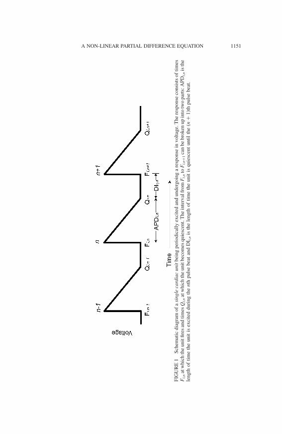
As shown in Fig. 1, each individual cardiac unit involves a point in time
F at which the unit “fires”, i.e. undergoes a sudden increase in voltage, and
a second point in time Q at which the cell becomes “quiescent”, i.e. the
voltage drops to zero. Each of these units fires repetitively, so we denote by
Fi, n the time at which the ith unit fires its nth pulse beat, and Qi, n as the time
at which ith unit becomes quiescent after the nth pulse beat. The duration
for which the ith unit has a non-zero voltage during its nth pulse beat is
denoted by APDi, n (for the action potential duration). The duration for
which the ith unit has a zero voltage during its nth pulse beat is denoted by
DIi, n (for the diastolic interval).
Our model is based on two experimental observations, which we take as
facts. The first fact is that for a single cardiac unit, the duration of an action
potential is solely determined by a single function of the previous
diastolic interval. That is, in terms of our model,
APDi; n ¼ f ðDIi; n21Þ: ð1Þ
The second experimental fact is that the speed of propagation of the nth
excitation signal from the ith unit to the (i þ 1)th unit is also solely
determined by a single function of the previous diastolic interval. We
denote this speed as CVi, n for conduction velocity and have therefore
CVi; n ¼ gðDIi; n21Þ: ð2Þ
Note that CVi, n refers only to the point in the cycle where the unit
becomes excited, i.e. where the voltage undergoes a sudden increase.
The governing equation for the chain can now be constructed. Each unit
is assumed to receive a signal from the unit to the left of it. The first unit in
the chain is being excited periodically by the experimenter, and we treat
this as a boundary condition, see below. Our derivation involves relating
the nth period of the ith unit, which we represent by Pi, n, to the nth period
of the (i þ 1)th unit Piþ1, n. It is evident that
Pi; n ¼ APDi; n þ DIi; n: ð3Þ
M.D. STUBNA et al.1150
FIG
UR
E1
Sch
emat
icd
iag
ram
of
asi
ng
leca
rdia
cu
nit
bei
ng
per
iod
ical
lyex
cite
dan
du
nd
ergo
ing
are
spo
nse
inv
olt
age.
Th
ere
spo
nse
con
sist
so
fti
mes
Fi,
nat
wh
ich
the
un
itfi
res
and
tim
esQ
i,n
atw
hic
hth
eu
nit
bec
om
esq
uie
scen
t.T
he
inte
rval
fro
mF
i,n
toF
i,nþ
1ca
nb
eb
rok
enu
pin
totw
op
arts
:A
PD
i,n
isth
ele
ngth
of
tim
eth
eu
nit
isex
cite
dd
uri
ng
the
nth
pu
lse
bea
tan
dD
I i,n
isth
ele
ng
tho
fti
me
the
un
itis
qu
iesc
ent
un
til
the
(nþ
1)t
hp
uls
eb
eat.
A NON-LINEAR PARTIAL DIFFERENCE EQUATION 1151
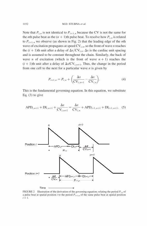
Note that Pi, n is not identical to Piþ1, n because the CV is not the same for
the nth pulse beat as the (n þ 1)th pulse beat. To resolve how Pi, n is related
to Piþ1, n we observe (as shown in Fig. 2) that the leading edge of the nth
wave of excitation propagates at speed CVi, n, so the front of wave n reaches
the (i þ 1)th unit after a delay of Dx=CVi; n: Dx is the cardiac unit spacing
and is assumed to be constant throughout the chain. Similarly, the back of
wave n of excitation (which is the front of wave n þ 1) reaches the
(i þ 1)th unit after a delay of Dx/CVi, nþ1. Thus, the change in the period
from one cell to the next for a particular wave n is given by
Piþ1; n ¼ Pi; n þDx
CVi; nþ1
2Dx
CVi; n
� �: ð4Þ
This is the fundamental governing equation. In this equation, we substitute
Eq. (3) to give
APDi; nþ1 þ DIi; nþ1 þDx
CVi; nþ1
¼Dx
CVi; n
þ APDiþ1; nþ1 þ DIiþ1; nþ1: ð5Þ
FIGURE 2 Illustration of the derivation of the governing equation; relating the period Pi,n ofa pulse beat at spatial position i to the period Piþ1,n of the same pulse beat at spatial positioni þ 1:
M.D. STUBNA et al.1152
Then, substituting Eqs. (1) and (2), defining hðxÞ ¼ Dx=gðxÞ and rewriting
ui; n ; DIi; n for clarity, results in
uiþ1; nþ1 þ f ðuiþ1; nÞ2 ui; nþ1 2 f ðui; nÞ þ hðui; nÞ2 hðui; nþ1Þ ¼ 0 ð6Þ
which is a partial difference equation on the dependent variable ui, n
with the independent variables i, n which indicate space and time,
respectively.
Although working with functions for f and h fitted directly from
experimental data is possible (see Fig. 3), we further simplify the
problem by taking f and h as idealized functions which give
similar qualitative behavior to the experimentally determined functions,
namely
f ðui; nÞ ¼ 21 þ mð1 2 ui; nð1 2 ui; nÞÞ; ð7Þ
hðui; nÞ ¼ aui; n þ b: ð8Þ
Extensive numerical simulations have shown that these functions
capture the essential details of the more complicated system. Notice that
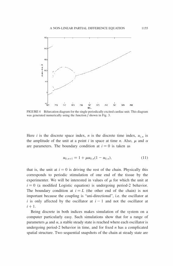
Eq. (7) is a variant on the well known Logistic equation, as might be
expected from the bifurcation diagram in Fig. 4 which looks similar to
the corresponding diagram for the Logistic equation. Thus, the governing
Here i is the discrete space index, n is the discrete time index, ui, n is
the amplitude of the unit at a point i in space at time n. Also, m and a
are parameters. The boundary condition at i ¼ 0 is taken as
u0; nþ1 ¼ 1 þ mu0; nð1 2 u0; nÞ; ð11Þ
that is, the unit at i ¼ 0 is driving the rest of the chain. Physically this
corresponds to periodic stimulation of one end of the tissue by the
experimenter. We will be interested in values of m for which the unit at
i ¼ 0 (a modified Logistic equation) is undergoing period-2 behavior.
The boundary condition at i ¼ L (the other end of the chain) is not
important because the coupling is “uni-directional”, i.e. the oscillator at
i is only affected by the oscillator at i 2 1 and not the oscillator at
i þ 1:
Being discrete in both indices makes simulation of the system on a
computer particularly easy. Such simulations show that for a range of
parameters m and a, a stable steady state is reached where each oscillator is
undergoing period-2 behavior in time, and for fixed n has a complicated
spatial structure. Two sequential snapshots of the chain at steady state are
FIGURE 4 Bifurcation diagram for the single periodically excited cardiac unit. This diagramwas generated numerically using the function f shown in Fig. 3.
A NON-LINEAR PARTIAL DIFFERENCE EQUATION 1155
shown in Fig. 5. As time n is incremented further, the pictures would just
repeat, since the overall behavior is period-2 in time.
The aim of our work on this problem is to understand the dynamics of the
system as shown in Fig. 5 through the use of perturbation techniques.
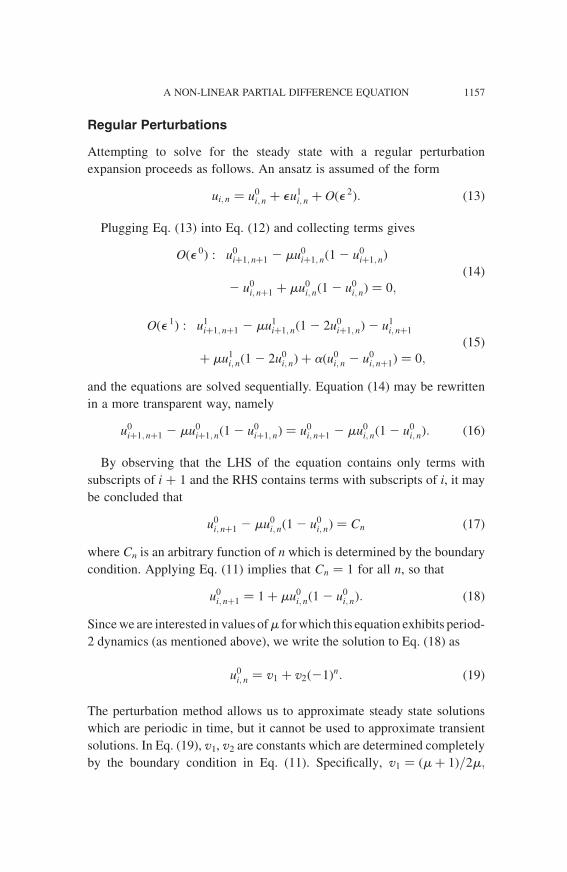
ANALYSIS
To begin with, we introduce a small parameter e into the problem by
assuming that a in Eq. (10) is small, and we replace a by ea:
nþ1 for ui, n, ui, nþ1 in Eq. (10), using Eq. (38), and denoting
uiþ1, n as uþn ; we have
uþnþ1 ¼ muþ
n ð1 2 uþn Þ þ ½v2
1 ð2mþ 1 þ mv21 Þ þ mðv2
2 Þ2�
þ ½2mv21 2 m2 2a2 1�v2
2 ð21Þn:ð40Þ
which is just an ordinary difference equation in n on uþn : By simulating
this equation for given parameters we can obtain information about the
solution that is missing from the slow-flow equations in the previous
section.
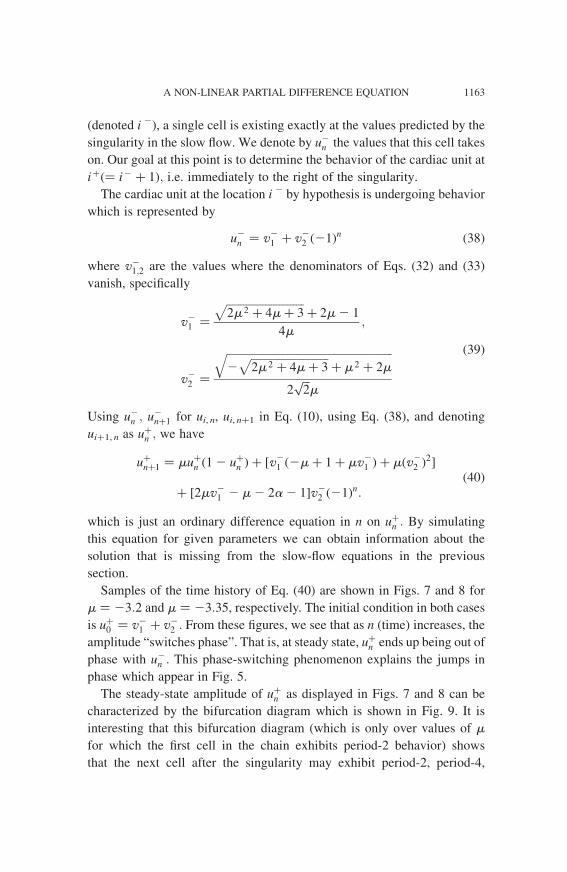
Samples of the time history of Eq. (40) are shown in Figs. 7 and 8 for
m ¼ 23:2 and m ¼ 23:35, respectively. The initial condition in both cases
is uþ0 ¼ v2
1 þ v22 : From these figures, we see that as n (time) increases, the
amplitude “switches phase”. That is, at steady state, uþn ends up being out of
phase with u2n : This phase-switching phenomenon explains the jumps in
phase which appear in Fig. 5.
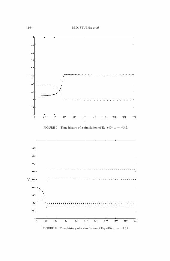
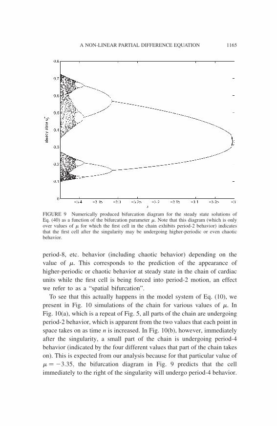
The steady-state amplitude of uþn as displayed in Figs. 7 and 8 can be
characterized by the bifurcation diagram which is shown in Fig. 9. It is
interesting that this bifurcation diagram (which is only over values of m
for which the first cell in the chain exhibits period-2 behavior) shows
that the next cell after the singularity may exhibit period-2, period-4,
A NON-LINEAR PARTIAL DIFFERENCE EQUATION 1163
FIGURE 7 Time history of a simulation of Eq. (40). m ¼ 23:2:
FIGURE 8 Time history of a simulation of Eq. (40). m ¼ 23:35:
M.D. STUBNA et al.1164
period-8, etc. behavior (including chaotic behavior) depending on the
value of m. This corresponds to the prediction of the appearance of
higher-periodic or chaotic behavior at steady state in the chain of cardiac
units while the first cell is being forced into period-2 motion, an effect
we refer to as a “spatial bifurcation”.
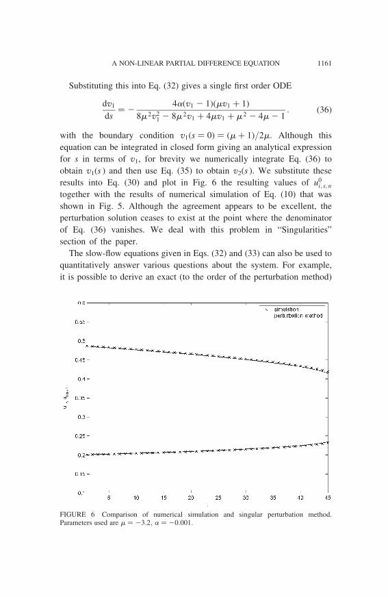
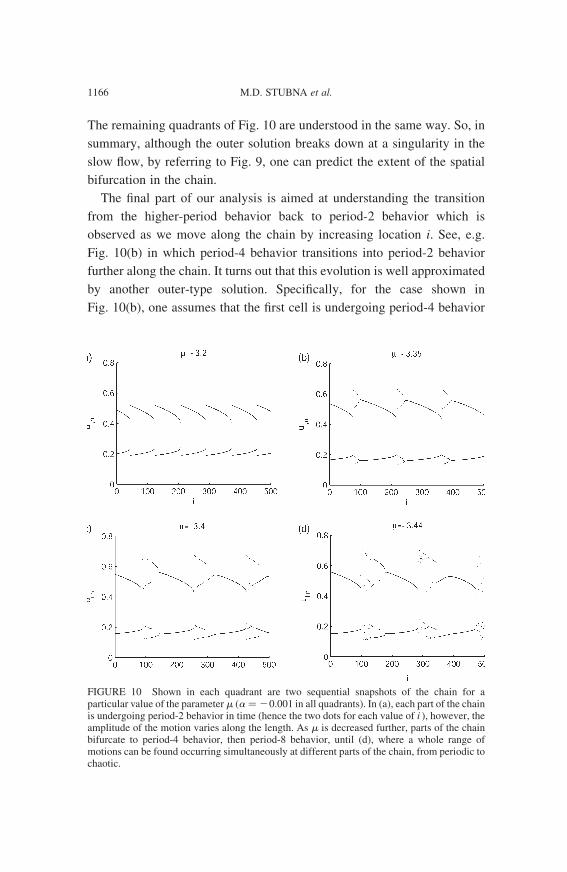
To see that this actually happens in the model system of Eq. (10), we
present in Fig. 10 simulations of the chain for various values of m. In
Fig. 10(a), which is a repeat of Fig. 5, all parts of the chain are undergoing
period-2 behavior, which is apparent from the two values that each point in
space takes on as time n is increased. In Fig. 10(b), however, immediately
after the singularity, a small part of the chain is undergoing period-4
behavior (indicated by the four different values that part of the chain takes
on). This is expected from our analysis because for that particular value of
m ¼ 23:35; the bifurcation diagram in Fig. 9 predicts that the cell
immediately to the right of the singularity will undergo period-4 behavior.
FIGURE 9 Numerically produced bifurcation diagram for the steady state solutions ofEq. (40) as a function of the bifurcation parameter m. Note that this diagram (which is onlyover values of m for which the first cell in the chain exhibits period-2 behavior) indicatesthat the first cell after the singularity may be undergoing higher-periodic or even chaoticbehavior.
A NON-LINEAR PARTIAL DIFFERENCE EQUATION 1165
The remaining quadrants of Fig. 10 are understood in the same way. So, in
summary, although the outer solution breaks down at a singularity in the
slow flow, by referring to Fig. 9, one can predict the extent of the spatial
bifurcation in the chain.
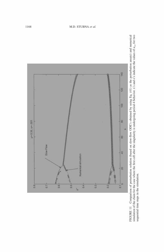
The final part of our analysis is aimed at understanding the transition
from the higher-period behavior back to period-2 behavior which is
observed as we move along the chain by increasing location i. See, e.g.
Fig. 10(b) in which period-4 behavior transitions into period-2 behavior
further along the chain. It turns out that this evolution is well approximated
by another outer-type solution. Specifically, for the case shown in
Fig. 10(b), one assumes that the first cell is undergoing period-4 behavior
FIGURE 10 Shown in each quadrant are two sequential snapshots of the chain for aparticular value of the parameter m (a ¼ 20.001 in all quadrants). In (a), each part of the chainis undergoing period-2 behavior in time (hence the two dots for each value of i ), however, theamplitude of the motion varies along the length. As m is decreased further, parts of the chainbifurcate to period-4 behavior, then period-8 behavior, until (d), where a whole range ofmotions can be found occurring simultaneously at different parts of the chain, from periodic tochaotic.
M.D. STUBNA et al.1166
and modifies the singular perturbation method appropriately. First, the new
perturbation ansatz (c.f. Eq. (30)) is taken to be
This form is chosen because it is possible to represent any period-4
motion by choosing appropriate values of v1,2,3,4. The rest of the
perturbation scheme is carried out exactly as above, with the exception
of when it comes to eliminating secular terms. The coefficients of the
constant term, and of the cos(np ), sin(np/2), and cos(np/2) terms must
all be set to zero, thus producing four coupled ODE’s. For brevity, these
are not reprinted here, but their numerical solution for m ¼ 23:35; a ¼
20:001 is shown in Fig. 11. As can be seen, the method captures the
transition from period-4 to period-2 behavior quite well, up until the
point where the next singularity is reached. In summary, by pasting
together outer solutions, along with the information provided by the
bifurcation diagram Fig. 9, the total dynamics of the chain can be
understood.
CONCLUSIONS
We have demonstrated, though the use of numerical simulations and
singular perturbation analysis, that the partial difference equation studied in
this work, Eq. (10), exhibits a “spatial bifurcation” structure at steady state.
That is, for certain parameter ranges, parts of the chain may be oscillating
in period-2 motion while other parts may be oscillating in higher periodic
motion or even chaotic motion. The spatial structure of the solution may be
understood as regions of outer solutions (from ODE’s) which are connected
together at singularities where the ODE’s break down. The behavior at the
singularities is understood through the use of Fig. 9 which predicts the
dynamics of the first cell to the right of the singularity for the given
parameter value(s).
The spatial bifurcation phenomenon observed in the present model is due
in part to a feature of the assumed form of the restitution function f in
Eq. (7), specifically that f is non-monotonic. Many experiments have shown
that real restitution functions can be non-monotonic, and hence the spatial
bifurcation structure that we observe may play an important role in
explaining complex cardiac rhythms that are observed experimentally.
A NON-LINEAR PARTIAL DIFFERENCE EQUATION 1167
FIG
UR
E1
1C
om
par
iso
no
fp
ertu
rbat
ion
solu
tio
n(b
ased
on
slow
-flow
OD
E’s
ob
tain
edb
yu
sin
gE
q.
(41
)as
the
per
turb
atio
nan
satz
)an
dn
um
eric
alsi
mu
lati
on
of
the
chai
nfo
rth
eca
sew
her
eth
efi
rst
cell
afte
rth
esi
ng
ula
rity
isu
nd
erg
oin
gp
erio
d-4
beh
avio
r.x
’san
do
’sin
dic
ate
the
val
ues
of
ui,
nfo
rtw
ose
qu
enti
alti
me
step
sin
the
sim
ula
tio
n.
M.D. STUBNA et al.1168
Extensions of this work could include the relaxation of certain
simplifying assumptions to obtain a model which is more biologically
realistic. This could include the inclusion of diffusion of current along the
chain, and/or a more realistic choice for the dispersion function used in
Eq. (8). See Refs. [2,9,10] for recent approaches which include the effects
of diffusion in models.
References
[1] D. R. Chialvo, R. F. Gilmour, Jr. and J. Jalife, Low dimensional chaos in cardiac tissue,Nature, 343 (1990), 653–657.
[2] B. Echebarria and A. Karma, Instability and spatiotemporal dynamics of alternans inpaced cardiac tissue., arXiv: cond-mat/0111552 v1, 2001.
[3] R. F. Gilmour, M. Watanabe and N. Otani, Restitution properties and dynamics ofreentry, Cardiac Electrophysiology: From Cell to Bedside, 3rd Ed., W. B. SaundersCompany, London, pp 378–385, 1999.
[4] M. R. Guevara, G. Ward, A. Shrier and L. Glass, Electrical alternans and period-doublingbifurcations, Comput. Cardiol., (1984), 167–170.
[5] M. H. Holmes, Introduction to Perturbation Methods, Springer-Verlag, New York,1995.
[6] R. E. Mickens, Difference Equations: Theory and Applications, Van Nostrand Reinhold,New York, 1990.
[7] R. J. Myerburg, K. M. Kessler, S. Kimura, A. L. Bassett, M. M. Cox andA. Castellanos, Life-threatening ventricular arrhythmias: the link between epidemiologyand pathophysiology, Cardiac Electrophysiology: From Cell to Bedside, 2nd Ed., W. B.Saunders Company, London, pp 723–731, 1995.
[8] N. F. Otani and R. F. Gilmour, Memory models for the electrical properties of localcardiac systems, J. Theor. Biol., 187 (1997), 409–436.
[9] A. Vinet, Quasiperiodic circus movement in a loop model of cardiac tissue: Multistabilityand low dimensional equivalence, Ann. Biomed. Eng., 28 (2000), 704–720.
[10] M. A. Watanabe, F. H. Fenton, S. J. Evans, H. M. Hastings and A. Karma, Mechanan-ism for discordant alternans, J. Cardiovasc. Electrophysiol., 12(2) (2001), 196–206.