ANALYSIS OF A PARTIAL DIFFERENTIAL
EQUATION MODEL FOR NECROTIZING
ENTEROCOLITIS
by
Mark D. Tronzo
B.S. in Mechanical Engineering, Geneva College, 1979
B.S. in Mathematics, Geneva College, 1979
M.S. in Engineering, Youngstown State University, 1986
M.S. in Mathematics, Youngstown State University, 2005
Submitted to the Graduate Faculty of
the Kenneth P. Dietrich School of Arts and Science in partial
fulfillment
of the requirements for the degree of
Doctor of Philosophy
University of Pittsburgh
2014
UNIVERSITY OF PITTSBURGH
KENNETH P. DIETRICH SCHOOL OF ARTS AND SCIENCE
This dissertation was presented
by
Mark D. Tronzo
It was defended on
March 14, 2014
and approved by
Prof. Ivan Yotov, Dept. of Mathematics, University of Pittsburgh
Prof. Catalin Trenchea, Dept. of Mathematics, University of Pittsburgh
Prof. David Swigon, Dept. of Mathematics, University of Pittsburgh
Prof. Jonathan Rubin, Dept. of Mathematics, University of Pittsburgh
Prof. Yoram Vodovotz, Dept. of Immunology, University of Pittsburgh
Dissertation Advisors: Prof. Ivan Yotov, Dept. of Mathematics, University of Pittsburgh,
Prof. Catalin Trenchea, Dept. of Mathematics, University of Pittsburgh
ii
ANALYSIS OF A PARTIAL DIFFERENTIAL EQUATION MODEL FOR
NECROTIZING ENTEROCOLITIS
Mark D. Tronzo, PhD
University of Pittsburgh, 2014
This thesis presents and analyzes a mathematical model for necrotizing enterocolitis (NEC), a
devastating disease that attacks the gastrointestinal tract of pre-term infants. Mathematical
models for NEC have been developed in the past. These modes are extremely valuable and
provide important insights into the disease. However, all of the models developed previously
are one dimensional, ordinary differential equation models and, therefore, simulate only the
transient effects of NEC but do not fully model its spatial effects. The mathematical model
presented here is a three dimensional model in the form of a system of nonlinear partial
differential equations. A three dimensional model is needed to accurately simulate diffusion
and advection of the major factors in NEC, to account for the different effects of NEC in
the different regions in the body, and to fully integrate all the effects of such mechanisms as
epithelial cell degradation and migration.
This thesis presents medical research regarding NEC, constructs inflammatory cascades
related to the disease, and develops the system of partial differential equation system. Also,
full mathematical analysis of the system of equations. The mathematical analysis of the
system of partial differential equations and the associated a mixed finite element analysis
are, perhaps, the most important parts of the thesis. The results of this analysis have
significance for the NEC system and have significance independent of the NEC system. For
example, existence, uniqueness, and regularity analysis is presented in the weak mixed form
for the coupled nonlinear equations:
iv
∂u1∂t
−∇ · (D1∇u1 − u1∇u2) = f1(u1, u2)
∂u2∂t
−∇ · (D2∇u2) = f2(u1, u2) (x, t) ∈ Ω× (0, T ]
∇u1 · n = 0 and ∇u2 · n = 0 on Γ
where f1 and f2 are nonlinear functions. Furthermore, finite element analysis (using the
mixed method) is done on this coupled system and convergence is proven, a new and very
important result. No mixed method finite element analysis has previously been published
for this system. Similar analysis is done on the rest of the partial differential equations in
the system. At the end of the thesis, computer simulations are done using the mathematical
model. These simulations demonstrate that the NEC mathematical model presented here
produces realistic results consistent with the actual progression of the disease.
v
Acknowledgements
I want to thank the members of my thesis committee for their help. I thank my adviser,
Ivan Yotov, for his great help, over several years, on the finite element analysis included in
this thesis. My co-adviser, Catalin Trenchea, provided very valuable help and insight on
the partial differential equation analysis part of this thesis. I would like to thank David
Swigon and Jonathan Rubin for carefully reading the first three chapters of this thesis and
providing many important suggestions to make the thesis better. Finally, I would like to
thank Yoram Vodovotz for his important corrections and suggestions with regard to the
medical and biological aspects of this thesis.
I want to also thank the many people who were of great help to me in many other ways
while at the University of Pittsburgh including my advisor on my previous research, Beatrice
Riviere. Molly Williams, Neale Hahn, Inna Sysoeva, and Frank Beatrous were of great help
to me in my academic and teaching development. I gained valuable experience while working
with many fellow graduate students including, especially, Milan Sherman, Johnny Kwong,
and Ken-Hsien Chuang.
I would like to take this time to thank the many, many people who helped me through-
out my undergraduate education and during my career in industry as an engineer. These
include Bruce Miller, Forrest Justis, and Stanley Reyle from Geneva College; Ed Robson
from the Reformed Presbyterian Theological Seminary; Richard W. Erickson and Richard
E. Merkle from Cooper Industries. I thank those co-workers who made my industrial expe-
rience more enjoyable including, especially, Chuck Chernicky, Ron Krystek, John Brundage,
Don Kockritz, and Carl Dahl.
More than all others on this earth I want to thank my parents, Thomas C. Tronzo and
Olga P. Tronzo, as well as my brother, Thomas M. Tronzo for their help and encouragement
throughout my life.
Thanks, above all, be to God, since He Himself gives to all people life and breath and all
things; (Acts 17:25 b) and to Jesus Christ who died for us so that we may have the assurance
of eternal life (I John 2:25). To Him be all the glory.
Mark D. Tronzo
vi
TABLE OF CONTENTS
1.0 NECROTIZING ENTEROCOLITIS . . . . . . . . . . . . . . . . . . . . . . 1
1.1 OVERVIEW OF THE DISEASE . . . . . . . . . . . . . . . . . . . . . . . 2
1.2 SMALL INTESTINE STRUCTURE AND FUNCTION . . . . . . . . . . . 3
1.3 Cells of the epithelium . . . . . . . . . . . . . . . . . . . . . . . . . . . . . 7
1.4 Important Mechanical and Physical Factors. . . . . . . . . . . . . . . . . 8
1.4.1 Cell Death and Renewal of the epithelium . . . . . . . . . . . . . . 8
1.4.2 Wound Healing . . . . . . . . . . . . . . . . . . . . . . . . . . . . . 12
1.4.3 Intestinal Peristalsis . . . . . . . . . . . . . . . . . . . . . . . . . . 19
1.4.4 Bacterial Translocation . . . . . . . . . . . . . . . . . . . . . . . . . 19
1.5 FACTORS CRITICAL TO NEC . . . . . . . . . . . . . . . . . . . . . . . 20
1.5.1 Affects of Prematurity . . . . . . . . . . . . . . . . . . . . . . . . . 20
1.5.2 Advantages of Breast Feeding vs. Formula Feeding in NEC . . . . . 23
1.5.3 Particular Advantages of Breast Feeding in case of Prematurity . . 28
1.6 Description of inflammatory cells, cytokines, and other factors in NEC . . 28
2.0 PREPARATIONS FOR CONSTRUCTION OF A NEC MODEL . . . 41
2.1 Inflammatory Cascade . . . . . . . . . . . . . . . . . . . . . . . . . . . . . 42
2.2 Physical Domain for the NEC model. . . . . . . . . . . . . . . . . . . . . . 48
2.3 General Inflammatory Cascade . . . . . . . . . . . . . . . . . . . . . . . . 49
2.4 A Typical Scenario . . . . . . . . . . . . . . . . . . . . . . . . . . . . . . . 54
3.0 A PARTIAL DIFFERENTIAL EQUATION MODEL FOR NEC . . . . 60
3.1 Derivation of Partial Differential Equations . . . . . . . . . . . . . . . . . . 61
3.2 The System of Partial Differential Equations . . . . . . . . . . . . . . . . . 71
vii
3.3 The NEC Equations in the Four Regions . . . . . . . . . . . . . . . . . . . 73
3.4 Suggested Changes . . . . . . . . . . . . . . . . . . . . . . . . . . . . . . . 73
4.0 ANALYSIS OF THE PDE SYSTEM . . . . . . . . . . . . . . . . . . . . . 75
4.1 Notation . . . . . . . . . . . . . . . . . . . . . . . . . . . . . . . . . . . . . 77
4.2 Analysis of PDEs in Part I . . . . . . . . . . . . . . . . . . . . . . . . 80
4.3 Existence and Regularity of Weak Mixed Solution for the Linear Problem . 81
4.3.1 Existence of Solution to Finite System. . . . . . . . . . . . . . . . . 82
4.3.2 Establish Bounds for Various Terms . . . . . . . . . . . . . . . . . 85
4.3.3 Convergence to a Solution of Linear Weak Mixed System . . . . . . 88
4.3.4 Regularity of Linear Weak Mixed System . . . . . . . . . . . . . . . 94
4.4 The nonlinear weak mixed system . . . . . . . . . . . . . . . . . . . . . . . 96
4.4.1 Development and Proof of nonlinear Theorems . . . . . . . . . . . 96
4.4.2 Uniqueness Mixed Weak Solution . . . . . . . . . . . . . . . . . . . 104
4.4.3 Application of the Theorems to Individual Equations . . . . . . . . 109
4.4.4 Conclusion . . . . . . . . . . . . . . . . . . . . . . . . . . . . . . . 118
4.5 Analysis of PDEs in Part II . . . . . . . . . . . . . . . . . . . . . . . . 119
4.5.1 Properties that apply to both the Non-Degenerate Case and the
Degenerate Case . . . . . . . . . . . . . . . . . . . . . . . . . . . . 121
4.5.2 Properties that apply only to Non-Degenerate Case . . . . . . . . . 122
4.6 Non-Degenerate Case - Existence of a solution. . . . . . . . . . . . . . . . 124
4.7 Degenerate Case . . . . . . . . . . . . . . . . . . . . . . . . . . . . . . . . 131
4.7.1 Degenerate Case - Regularity . . . . . . . . . . . . . . . . . . . . . 132
4.7.2 Degenerate Case - Regularity of the Weak Form . . . . . . . . . . . 133
4.8 Analysis of PDEs in Part III . . . . . . . . . . . . . . . . . . . . . . . 136
5.0 FINITE ELEMENT ANALYSIS (CONVERGENCE ANALYSIS FOR
THE FULLY COUPLED SYSTEM OF PDES) . . . . . . . . . . . . . . . 138
5.1 Conditions and Notation for FEM Section. . . . . . . . . . . . . . . . . . . 142
5.2 Finite Element Analysis of the PDEs in Part I . . . . . . . . . . . . . . . . 146
5.3 Finite Element Analysis of the PDEs in Part II . . . . . . . . . . . . . . . 179
5.3.1 Analysis of semi-discrete scheme . . . . . . . . . . . . . . . . . . . 182
viii
5.4 Finite Element Analysis of the PDEs in Part III . . . . . . . . . . . . . . . 196
5.5 Conclusion for Finite Element Analysis Chapter . . . . . . . . . . . . . . . 201
6.0 CONVERGENCE TESTS . . . . . . . . . . . . . . . . . . . . . . . . . . . . 204
6.1 Code to test coupled Advection equation . . . . . . . . . . . . . . . . . . . 204
6.1.1 Implicit Finite Difference . . . . . . . . . . . . . . . . . . . . . . . . 204
6.1.2 Explicit Finite Difference . . . . . . . . . . . . . . . . . . . . . . . 214
6.1.3 Cell-Centered Finite Difference Method . . . . . . . . . . . . . . . . 215
6.2 Test Runs . . . . . . . . . . . . . . . . . . . . . . . . . . . . . . . . . . . . 217
7.0 SIMULATION RESULTS . . . . . . . . . . . . . . . . . . . . . . . . . . . . 227
7.1 Normal Case - Term Infant, No Injury to the epithelium. . . . . . . . . . . 228
7.2 Case - Prematurity, No Injury to the epithelium. . . . . . . . . . . . . . . . 229
7.3 Case - Term Infant, Partial Injury to epithelium. . . . . . . . . . . . . . . 231
7.4 Case - Term Infant, Total Injury to epithelium. . . . . . . . . . . . . . . . 248
7.5 Summary of Simulations . . . . . . . . . . . . . . . . . . . . . . . . . . . . 253
7.6 Conclusions . . . . . . . . . . . . . . . . . . . . . . . . . . . . . . . . . . . 257
7.7 A Computational Note of the Application of the NEC Equations to Different
Domains . . . . . . . . . . . . . . . . . . . . . . . . . . . . . . . . . . . . . 258
8.0 CONCLUSIONS AND FUTURE WORK . . . . . . . . . . . . . . . . . 260
APPENDIX A. FEM ANALYSIS PART II NON-DEGENERATE CASE . 263
APPENDIX B. RENAMING OF PARAMETERS . . . . . . . . . . . . . . . 265
APPENDIX C. LIPSCHITZ CONTINUITY RELATED TO PDES IN PART
I . . . . . . . . . . . . . . . . . . . . . . . . . . . . . . . . . . . . . . . . . . . . 269
APPENDIX D. VERTICAL GRAPHS FOR THE SIMULATION CHAP-
TER. . . . . . . . . . . . . . . . . . . . . . . . . . . . . . . . . . . . . . . . . . 276
BIBLIOGRAPHY . . . . . . . . . . . . . . . . . . . . . . . . . . . . . . . . . . . . 280
ix
LIST OF TABLES
1 Affects of prematurity and the corresponding advantages of breast feeding. . . 29
2 Regularity of the weak solution of the NEC PDE system. . . . . . . . . . . . 137
3 Convergence Rates for fully coupled system (1 of 2). . . . . . . . . . . . . . . 202
4 Convergence Rates for fully coupled system (2 of 2). . . . . . . . . . . . . . . 203
5 Renaming of parameters (1 of 3). . . . . . . . . . . . . . . . . . . . . . . . . . 266
6 Renaming of parameters (2 of 3). . . . . . . . . . . . . . . . . . . . . . . . . . 267
7 Renaming of parameters (3 of 3). . . . . . . . . . . . . . . . . . . . . . . . . . 268
x
LIST OF FIGURES
1 Representation of intestinal villi and crypts. . . . . . . . . . . . . . . . . . . . . . . 4
2 Representation of the epithelium. . . . . . . . . . . . . . . . . . . . . . . . . . . . 5
3 Cells of the epithelium . . . . . . . . . . . . . . . . . . . . . . . . . . . . . . . . 9
4 Function of Paneth Cells. . . . . . . . . . . . . . . . . . . . . . . . . . . . . . . . 9
5 Cell Shedding. . . . . . . . . . . . . . . . . . . . . . . . . . . . . . . . . . . . . 11
6 Cell Motility . . . . . . . . . . . . . . . . . . . . . . . . . . . . . . . . . . . . . 14
7 Villus Contraction . . . . . . . . . . . . . . . . . . . . . . . . . . . . . . . . . . 15
8 Tight Junction, Adherens, Cadherins, Integrins. . . . . . . . . . . . . . . . . . . . . 16
9 Factors in Epithelial Restitution. . . . . . . . . . . . . . . . . . . . . . . . . . . . . 17
10 Disruption and restoration of the epithelium. . . . . . . . . . . . . . . . . . . . . . . 18
11 Intestinal Peristalsis. . . . . . . . . . . . . . . . . . . . . . . . . . . . . . . . . . 19
12 Three important pathways of bacteria from the lumen into the tissue. . . . . . . . . . . 21
13 Advantages of Breast Feeding. . . . . . . . . . . . . . . . . . . . . . . . . . . . . . 24
14 Results of TLR4 signalling. . . . . . . . . . . . . . . . . . . . . . . . . . . . . . . 39
15 Partial Inflammatory Cascade. . . . . . . . . . . . . . . . . . . . . . . . . . . . . . 43
16 PAF’s role in the inflammatory cascade . . . . . . . . . . . . . . . . . . . . . . . . 44
17 Disruption and restoration of the epithelium. . . . . . . . . . . . . . . . . . . . . . . 45
18 Other factors involved in epithelial restitution/proliferation. . . . . . . . . . . . . . . . 46
19 This diagram shows how the presence of nitric oxide and IFN-γ results in
epithelial layer permeability. . . . . . . . . . . . . . . . . . . . . . . . . . . . 49
20 This diagram shows the four regions that will be used in the NEC mathematical
model. . . . . . . . . . . . . . . . . . . . . . . . . . . . . . . . . . . . . . . . 50
xi
21 General Inflammatory Cascade. . . . . . . . . . . . . . . . . . . . . . . . . . . . . 53
22 A typical NEC scenario (1 of 3). . . . . . . . . . . . . . . . . . . . . . . . . . . . . 56
23 A typical NEC scenario (2 of 3). . . . . . . . . . . . . . . . . . . . . . . . . . . . . 57
24 A typical NEC scenario (3 of 3). . . . . . . . . . . . . . . . . . . . . . . . . . . . . 58
25 Damage Production Term . . . . . . . . . . . . . . . . . . . . . . . . . . . . . . . 67
26 Buckley-Leverett equation, , q = 2, 4, 8. . . . . . . . . . . . . . . . . . . . . . . . . . 69
27 Buckley-Leverett equation, q = 1/2, 1/4, 1/8. . . . . . . . . . . . . . . . . . . . . . . 69
28 Normal Case - Term Infant, No Injury to the epithelium (1 of 2). . . . . . . . . . . . . 230
29 Normal Case - Term Infant, No Injury to the epithelium (2 of 2). . . . . . . . . . . . . 230
30 Simulation for Prematurity, No Injury, Formula Fed kpp = .05, bmax = 5 (1 of 2). . . . . . 232
31 Simulation for Prematurity, No Injury, Formula Fed kpp = .05, bmax = 5 (2 of 2). . . . . . 233
32 Simulation for Prematurity, No Injury, Formula Fed kpp = .05, bmax = 5. . . . . . . . . . 234
33 Simulation for Prematurity, No Injury, Breast Fed kpp = .5, bmax = 5 (1 of 2). . . . . . . 235
34 Simulation for Prematurity, No Injury, Breast Fed kpp = .5, bmax = 5 (2 of 2). . . . . . . 236
35 Simulation results for Prematurity, No Injury, Breast Fed kpp = .5, bmax = 5. . . . . . . . 237
36 Simulation results for Prematurity, No Injury, Breast Fed kpp = .7, bmax = 5 (1 of 2). . . . 238
37 Simulation results for Prematurity, No Injury, Breast Fed kpp = .7, bmax = 5 (2 of 2). . . 239
38 Simulation results for Prematurity, No Injury, Breast Fed kpp = .7, bmax = 5. . . . . . . . 240
39 Simulation for Prematurity, No Injury, Breast Fed kpp = 1, bmax = 5 (1 of 2). . . . . . . 241
40 Simulation for Prematurity, No Injury, Breast Fed kpp = 1, bmax = 5 (2 of 2). . . . . . . 242
41 Simulation for Prematurity, No Injury, Breast Fed kpp = 1, bmax = 5. . . . . . . . . . . 243
42 Comparison between formula fed and breast fed for prematurity and no injury. . . . . . . 244
43 Simulation results for Case Partial Injury, Formula Fed. . . . . . . . . . . . . . . . . . 246
44 Case - Partial Injury Formula Fed. The purpose of this figure is to give an average visual
picture of what is happening physically. . . . . . . . . . . . . . . . . . . . . . . . . 247
45 Simulation results for Case Partial Injury, Breastfed, kpp = .7. . . . . . . . . . . . . . . 248
46 Wound Closing for Case Partial Injury, Formula Fed. . . . . . . . . . . . . . . . . . . 249
47 Wound Closing for Case Partial Injury, Breastfed. . . . . . . . . . . . . . . . . . . . 249
48 Comparison between formula fed and breast fed for term infant and partial injury. These
graphs show the epithelial layer. . . . . . . . . . . . . . . . . . . . . . . . . . . . . 249
xii
49 Simulation results for Case Total Injury, Formula Fed. . . . . . . . . . . . . . . . . . 251
50 Simulation results for Case Total Injury, Breast Fed kpp = .7. . . . . . . . . . . . . . . 252
51 Wound Closing for Case Total Injury, Breast Fed kpp = .7. . . . . . . . . . . . . . . . 252
52 Simulation results for Case Total Injury, Breast Fed kpp = .000125. . . . . . . . . . . . 254
53 Simulation results for Case Total Injury, Breast Fed kpp = 1.25. . . . . . . . . . . . . . 255
54 Tissue Damage for Case Total Injury. . . . . . . . . . . . . . . . . . . . . . . . . . 256
55 The computational domain, discretized into grid of computational cells. . . . . . . . . . 259
56 Normal Case - Term Infant, No Injury to the epithelium. . . . . . . . . . . . . . . . . 276
57 Simulation results for Case Partial Injury, Formula Fed. . . . . . . . . . . . . . . . . . 277
58 Simulation results for Case Partial Injury, Breastfed. kpp = .7. . . . . . . . . . . . . . . 277
59 Simulation results for Case Total Injury, Formula Fed. . . . . . . . . . . . . . . . . . 278
60 Simulation results for Case Total Injury, Breast Fed kpp = .7. . . . . . . . . . . . . . . 278
61 Simulation results for Case Total Injury, Breast Fed kpp = .000125. . . . . . . . . . . . 278
62 Simulation results for Case Total Injury, Breast Fed kpp = 1.25. . . . . . . . . . . . . . 279
xiii
1.0 NECROTIZING ENTEROCOLITIS
Necrotizing Enterocolitis(NEC) is a devastating and often fatal disease that attacks the gas-
trointestinal tract of newborns. NEC is characterized by intestinal inflammation, intestinal
tissue death including destruction of the intestine, and sepsis. NEC most often attacks
preterm infants. Ironically, as the survival rate of preterm infants increases, so does the
incidence of NEC. NEC is diagnosed in about 2 out of 1000 live births per year [6]. NEC
occurs in approximately 7% of those infants with birth weights between 1 and 3 pounds.
The overall death rate among those infants diagnosed with NEC is between 20% and 30%
[101].
The purpose of this thesis is twofold. First of all this work presents a three dimensional
mathematical model of Necrotizing Enterocolitis(NEC). This model consists of a system of
partial differential equations (PDE) that models both the temporal and spatial aspects of
NEC. Secondly, this work analyses that NEC PDE system. That is, existence, uniqueness,
and regularity analysis is done on the entire PDE system. Also, a mixed finite element
analysis is done on the system of equations. This second purpose has significance for the
NEC PDE system and it has significance independent of the NEC PDE system. For the
NEC system, this analysis provides a strong mathematical foundation for the equations and
their interrelation with each other. On the other hand, some of the classes of equations in
the NEC PDE system occur, in a slightly different form, in other contexts but, in some cases,
no existence, uniqueness, and regularity results for these equations exist in the literature.
Even more importantly, the mixed finite element analysis presented later contains some new
and very significant results.
This first chapter will investigate much of the current medical research regarding NEC
in order to accumulate information for creating the NEC model. Much more material will
1
be presented in this chapter than will ultimately be used to build the model. This additional
material is included for a number of reasons. First of all, when constructing the NEC model it
is important to weigh all of the factors involved in NEC in order to decide what will and what
will not be included in the model. This can only be done after each mechanism and player in
the disease is investigated and evaluated in order to determine its importance to the model.
Therefore, much information is presented in this chapter and, then, in chapter two, the
evaluation process will be done and the factors to be included in the model will be determined.
Secondly, even though some of this material will not be used directly in the NEC model, the
material will still be used as a guide for setting simulation runs. Therefore, this material
will be of great help for creating realistic the initial conditions for the computer simulations
presented in chapter seven as well as for computer simulations in the future. Finally, the
additional material will provide background and motivation for a more advanced, extensive
NEC model in the future. This will be particularly relevant as new medical discoveries come
to light.
1.1 OVERVIEW OF THE DISEASE
NEC usually attacks the intestines resulting in severe, often irreparable damage. Bacteria
from the lumen may pass through the protective epithelial cells that line the intestines and
seeps into the underlying tissue. This triggers an inflammatory response within and around
the intestines that involves bacteria, macrophages, neutrophils, cytokines, as well as many
other biological components. If this inflammatory response is left unchecked it will cause
tissue death and, ultimately permanent damage to the intestine.
The causes of NEC are multifaceted. The main risk factor for NEC appears to be
prematurity - the more premature, the higher the risk for NEC. Formula feeding is another
risk factor for NEC which may also contribute to the disease once the disease has been
initiated. As mentioned above, the translocation of bacteria from the lumen to the underlying
tissue of the intestine is a critical factor in NEC, as well as the breakdown of the epithelial
layer of cells that protect the intestines. Many of these causes of NEC are interrelated and it
2
is not always clear which of these factors is most involved in initiating the disease and which
are secondary responses. These causes, their effects, and the physical mechanisms involved
will now be investigated.
1.2 SMALL INTESTINE STRUCTURE AND FUNCTION
In general, Necrotizing Enterocolitis strikes the gastrointestinal tract. Usually, NEC may
attack either the small or large intestine but the effects of NEC discussed in this thesis
will usually apply in either case. In this thesis, the small intestine will be used as the
representative organ of the GI tract that NEC attacks. Therefore,it will be worthwhile to
study the structure and function of the small intestine in some detail.
The study will begin by considering the components of the small intestine that are
directly affected by NEC. The open passage way of the GI tract in the small intestine will
here be referred to as the lumen. The interior radial surface on the lumen side of the small
intestine is covered with finger-like projections called villi (singular:villus). Throughout the
thesis, the villi will be represented by figure 1. These villi are covered by a gel layer called
mucus. On the outer part of the villi is a layer of cells called the epithelium. The epithelium
is supported below by the basal lamina or extracellular matrix (ECM). In the central portion
of each villus is the lamina propria. These (the mucus layer, the epithelium, the extra cellular
matrix, and the lamina propria) together make up what is called the mucosa.
The mucosa is responsible for functions critical for digestion such as absorption (of
nutrients) and secretion (of mucus). The epithelium is a layer of connected cells that
covers the villi and protects the underlying tissue. Throughout the thesis, the epithelium
will be represented by figure 2. These cells move at approximately 5-10 µm per hour and the
cells are renewed every 2 to 5 days [64]. The cells of the epithelium are primarily enterocytes,
which absorb nutrients and transfer these nutrients into the underlying tissue. Also included
in the epithelium are some goblet cells, which secrete mucus (a thick fluid which serves are a
protective layer for the epithelium) as well as intraepithelial lymphocytes (IELs). The small
intestine contains one IEL for every four to nine epithelial cells [35]. The regions between
3
Figure 1: Representation of intestinal villi and crypts. Throughout this thesis, the intestinal villi andcrypts will be represented by diagrams similar to this one.
the villi are called the crypts (see figure 1). In the crypts are found Paneth cells, which play
an important defensive role. Paneth cells secrete a wide variety of antimicrobial proteins
and peptides, such as lysozyme and phospholipase α-defensins, that fight many types of
bacteria, viruses, and fungi [106]. They are stimulated to secrete defensins when exposed to
bacteria or lipopolysaccharides (LPS) [100]. Paneth cells are also believed to play a major
role in protecting epithelial cell proliferation - the Paneth cells’ location adjacent to the
crypts is an ideal place from which they may protect stem cells from invading bacteria [106],
[100]. Between the enterocytes are tight junction proteins (see figure 2), which serve as a
barrier that keeps pathogens from passing from the lumen into the underlying tissue, and
gap junction proteins, which are important for cell-cell communication.
4
Figure 2: Representation of the epithelium. (This is the region of figure 1 that is enclosed by the rectangle.)Throughout this thesis, the epithelium will be represented by diagrams similar to this one.
The mucus layer consists of mucus which is made up of water, lipids, and mucin [6].
Mucins are glycoproteins produced by goblet cells and have the ability to form viscoelastic
gels [6], [35]. Mucins provide lubrication and protection of the epithelium from mechanical
damage caused by dietary constituents [91]. Mucus forms a continuous covering for the villi.
The average mucus layer thickness for the three major sections of the small intestines have
been determined to be 170 µm for the duodenum, 123 µm for the jejunum, and 480 µm for
the ileum [11]. The mucus layer is the site at which the body first encounters gut bacteria
[31]. All bacteria, including commensal bacteria, increase mucus production [60]. The mucus
layer serves as protection for the epithelium. Particles, bacteria, and viruses are trapped in
the mucus layer and, eventually expelled before they reach the underlying epithelium [131],
[140]. Mucus also keeps antimicrobial compounds near the epithelium where they may kill
some of the entrapped organisms [140]. Since mucus is continuously created and expelled
from the body, any material trapped in the mucus layer, including pathogenic bacteria, is
swept away with the exiting mucus [140]. The mucus layer is also a reservoir for secretory
immunoglobulin A (IgA). Secretory IgA’s bind pathogen and prevents attachment to the
5
epithelial cells [131].
The mucus layer greatly aids digestion. Mucus forms a constant, unstirred layer thereby
keeping digestive enzymes near the epithelium where they may aid normal absorbtion [91].
Molecules in the unstirred layer are, therefore, not taken away by peristalsis [128], [91]. (See
discussion of peristalsis later in this chapter.) In addition, mucins lower the diffusion of
large pathogenic bacteria but allows the passage of the smaller nutrient molecules [100]. It is
most beneficial for the host that the mucus layer be populated by normal flora or indigenous
bacteria, that is, the bacteria that is common to that particular host. This bacteria is often
referred to as commensal bacteria.
An important resident in the mucus layer is commensal bacteria. Commensal Bacteria
or Normal Flora plays a protective, beneficial role in the Mucus Layer. The human gut con-
tains between 10 x 1012 and 100 x 1012 organisms per ml of this commensal bacteria [35],[10].
Whenever it is operating properly, the immune system recognizes commensal bacteria and,
therefore, such bacteria does not illicit an inflammatory response. The commensal bacteria
protects by: 1) Competing with harmful bacteria for essential nutrients 2) Competing with
harmful bacteria for attachment sites 3) Producing substances that kill harmful bacteria
[35]. Commensal bacteria also facilitates the digestion, absorption and storage of certain
nutrients that would not otherwise be accessible to the host [10], [91].
While population of the mucus layer with commensal bacteria is beneficial to the host, fix-
ation of pathogenic bacteria in the mucus may be good or bad, as Montage [91] points out.
Whenever pathogenic bacteria is fixed in the mucus, it cannot reach the underlying epithelial
cells and, as long as there are only small amounts of trapped bacteria, the bacteria will be
removed together with the mucins during the normal mucus erosion process. On the other
hand, if the pathogenic bacterial accumulation in the mucus is at very high levels, so that it
exceeds the normal turnover rate of the mucus, then bacterial colonization occurs eventually
leading to infection and/or damage to the underlying epithelium [91].
The epithelium lies on what is called basal lamina or the extra cellular matrix (ECM).
(The ECM may be seen in figure 2.) The extra cellular matrix consists primarily of the pro-
tein collagen, elastin, fibronectin. Collagen provides strength to the extra cellular matrix.
6
Fibronectin binds the epithelial cells to the extracellular matrix and guides cell migration
[3].
The lamina propria mucosae is the tissue section that lies beneath the epithelium and
extra cellular matrix (see figure 2). It consists of smooth muscle cells and fibroblasts [35]. The
lamina propria mucosae has been described as ’loose’ connective tissue because it does not
have a large amount fibrous reinforcement that characterizes more dense connective tissue.
Loose connective tissues are easily distorted. Such tissues may move freely with respect to
one another.[103] Among the important cells found in the lamina propria are macrophages
and dendritic cells [60], [35].
1.3 CELLS OF THE EPITHELIUM
Enterocytes. The majority of cells on the external surface of the small intestine are ente-
rocytes. Enterocytes are formed in the crypts and move out toward the villus tips. These
column shaped cells (these are the yellow cells in figures 2 and 3) are responsible for di-
gestion and absorption of nutrients. They transfer substances from the intestinal lumen to
the circulatory system. They also obstruct bacteria from entering the underlying lamina
propria. Enterocytes release inflammatory cytokines such as IL-6, IL8, and TNF-α and
anti-inflammatory cytokines IL-10 and IL-15 [96]. Intestinal enterocytes also secrete anti-
microbial peptides such as defensins, cathelicidins, and calprotectins [10].
On top of the enterocytes is the actin-rich microvillar extension surface known as the
brush border (see figure 3). The brush border serves to impede microbial attachment
and invasion. It contains digestive enzymes and transporter systems involved in uptake and
metabolism [10].
Goblet Cells. Goblet cells secrete mucus that covers and protects the epithelium (see
figure 3). Goblet cells mature in the crypts and, after maturation, travel for 5-7 days to
the villus tips. When necessary these cells will secrete large amounts of mucus in response
to bacterial insult [100]. Goblet cells have the ability to secrete mucins that promote colo-
7
nization by commensal bacteria. Also, there is evidence that goblet cells, after coming into
contact with specific pathogenic bacteria, can produce mucus to which that bacteria will
bind. This will prevent the bacteria from binding to enterocytes [31].
M-Cells. These are specialized epithelial cells that lie over the Peyer’s Patch and lym-
phoid follicles. (The Peyer’s Patch consists of bundles of lymphatic tissue. See figure 3.
The Peyer’s Patch plays some role, not yet fully known, in immune response.) Unlike other
epithelial cells, M cells do not have long, fully developed microvilli (microvilli are the small
fingerlike projections on the top surface of many cells) and they lack certain surface glyco-
proteins. Instead, their microvilli are short and irregular. All of this means that antigen
have easy access to the apical surface of M cells. In fact, the primary function of M cells is
to transport material from the lumen, across the epithelium, to the underlying tissue [28].
In particular, M-Cells constantly sample the contents of the lumen and deliver antigen to
cells in the underlying tissue where inflammatory cells will be recruited if necessary [10].
Paneth Cells. These cells originate in the crypt stem cell region (see figure 4) but un-
like enterocytes, goblet, and M cells, Paneth cells move down toward the base of the crypts
[100]. Paneth cells secrete antimicrobial peptides and play a general defensive role. These
peptides apparently play a key role in destroying pathogenic bacteria while promoting col-
onization of favorable bacteria. Therefore, the proper functioning of Paneth cells is critical
for intestinal homeostasis [18].
1.4 IMPORTANT MECHANICAL AND PHYSICAL FACTORS.
1.4.1 Cell Death and Renewal of the epithelium
Cell death is an ongoing event of the epithelium. This death may be due to natural causes
or due to injury. Three types of cell death have been identified:
1. Apoptosis (Programmed Cell Death). This is cell death in an organized, well co-
8
Figure 3: Cells of the epithelium. (This figure is similar to figure 2 but shows different detail.) Thebrush border on enterocytes prevents microbes from attaching to the enterocytes. Goblet cells secretemucins. Mucus (mucins) helps to provide lubrication and protection for the epithelium. Mucus also keepenzymes near the epithelium, away from the effects of intestinal peristalsis, so that the enzymes may beeasily absorbed. M-Cells constantly sample the lumenal contents and transport bacteria (gram-positive andgram-negative bacteria) to the underlying Peyer’s patch.
Figure 4: Function of Paneth Cells. Paneth Cells are located in a strategic defensive position near thecrypts. There these cells are able to defend the stem cells located in the crypts. Paneth cells secreteantimicrobial peptides that destroy pathogenic bacteria and promote colonization by beneficial bacteria.
9
ordinated fashion followed by an organized removal of the dying cells. Apoptosis is usually
timely and desirable as it removes malfunctioning, senescent, or potentially dangerous cells.
However, if apoptosis occurs at too high a rate, the epithelial barrier function may be com-
promised [122]. It is not clear what causes apoptosis but TNF has been implicated as a
major factor in cell apoptosis/cell shedding [58].
2. Cell Shedding (Cell Suicide). Cell shedding is usually restricted to the surface cells
or villus tip cells where cells are loosely attached and may be easily shed into the lumen.
This shedding may involve single cells or sheets of cells [44]. It must be noted that some
believe that cell shedding is the result of apoptosis and, therefore, should not be classified
as a distinct form of cell death. On the other hand, others have observed that cell shedding
regularly occurs even among cells that have no evidence of initiation of apoptosis [138].
3. Cell Necrosis. This may be the result of injury and is characterized by the rapid
breakdown of the membrane integrity. The result is the release of cellular contents which
may damage nearby cells and create an unwanted cellular response. For example, HMGB1,
which is known to activate TLR4, is often released from damaged cells [44],[122].
An important mechanism in the small intestine is the process of renewal of the epithe-
lium. Under normal circumstances, intestinal epithelial cell turnover in nonhuman mammals
is about 2 days for adults but 4-5 days for infants [100]. In the absence of injury, cells are
shed at the villus tips and they are replaced by cells migrating up the villus from the crypts.
As a cell is in the process of being shed it induces its neighboring cells to shed and, in fact,
these neighboring cells shed about 5-10 minutes later [48]. In this way, the epithelium is
constantly renewed.
There are times during which epithelial cells shed at a higher rate than the rate at which
new cells move in to replace them. The result is that there are often gaps in the epithelium.
A paper published in 2005 indicated that about 3 % of the epithelium does not have cells
covering it at any given time [138]. This result appears to have been widely accepted,
however, a more recent study indicates that these gaps amount to a little less than 1 %
of the epithelium [48]. Either of these estimates would suggest that large passages exist in
the epithelium through which pathogenic bacteria might easily pass. Yet, during this entire
process of cell shedding and replacement, the epithelial barrier function is maintained, i.e.,
10
Figure 5: Cell Shedding. The top row shows the top view of the epithelium and the bottom row shows theside view of the epithelium. 1.) An actin/myosin ring forms around and under the dying cell (the dying cellis colored gray). 2.) This actin/myosin ring begins to contract and, thereby, begins to force the dying cell upand out of the epithelium [118]. At the same time, neighboring cells begin to move under the dying cell andtight junctions begin to redistribute under the cell (see Guan,[48]). 3.) The dying cell is forced completelyout of the epithelium and the tight junction proteins seal the resulting gap.
11
the epithelium remains sealed. This can be explained by either (1) cytoplasmic extensions
from neighboring cells, (2) an extracellular substance is secreted, perhaps by neighboring
epithelial cells, that fills the gap [138], (3) tight junction proteins will form connections
between the cells neighboring the departing cell [48]. The most recent research favors a
combination of (1) and (3): As a cell leaves the epithelium, its neighboring cells move in
underneath the dying cell and ZO1 (a tight junction protein) redistribution occurs. This
redistribution seals the gap created by the shed cell [48].
Therefore, current knowledge suggests the following model for cell shedding and the
continued maintenance of the epithelium: First, an actin/myosin ring forms around and
under the dying cell. Secondly, this actin/myosin ring begins to contract and, thereby, begins
to force the dying cell up and out of the epithelium [118]. At the same time, neighboring
cells begin to move under the dying cell and tight junctions begin to redistribute under the
cell [48]. Thirdly, the dying cell is forced completely out of the epithelium and the tight
junction proteins seal the resulting gap. (This model is illustrated in figure 5.)
1.4.2 Wound Healing
NEC is usually accompanied by some injury to the epithelium. Any injury to the epithelium
reduces its barrier function, thereby bacteria and other toxins may invade the underlying tis-
sue causing sustained inflammation to the host. Rapid and efficient resealing of the wounded
area is, therefore, essential to full recovery from NEC. Proper wound healing depends upon
many factors including proper cell migration, proliferation, and differentiation as well as
restoration of tight junctions between the cells [94]. Some important features of these pro-
cesses will be mentioned here.
After injury to the small intestine epithelium, a number of processes (processes which
may overlap) go into motion. 1 Villus Contraction. Almost simultaneous with the injury,
the villus dramatically contracts. This contraction greatly reduces the wounded area, thereby
aiding the healing process. 2 Within minutes after the injury, epithelial cell restitution
begins. Epithelial cells adjacent to the injured area begin to migrate to cover the exposed
area. This process does not usually involve cell proliferation. 3 About 18-24 hours after
12
injury, cell proliferation occurs in the crypts. This replenishes cells lost during injury.
4 The final, and essential, step in repairing the epithelium and all of its functions is the
restoration of tight junctions [19], [82].
1. Villus Contraction A most interesting feature of wound healing in the small intes-
tine is the phenomenon of villus contraction which greatly aids restitution. After an injury,
the villus actually contracts to reduce the surface area that needs to be resealed by epithelial
cells. (see figure 7) Specifically, the villus contracts enough to reduce the ”open area” by
about one half. It has been discovered that one large contraction of the villus occurs imme-
diately after injury. After that, the villus continues to contract, albeit at a slower rate, in
the hours following the injury [92].
2. Restitution Wound healing depends upon the cells’ ability to move across the
extracellular matrix. Immediately after injury, the cells adjacent to the wound begin to
migrate in order to cover the exposed part of the ECM. The leading edge of the cell flattens
and stretches forward attaching to the ECM at some point of the uncovered area of the
wound. In the process of stretching and reaching, elastic forces are generated in the cell.
These elastic forces cause the back of the cell to detach from the ECM. The cell then contracts
and the process is repeated. (see figure 6).
The attachment to the ECM is accomplished by activated integrins located at the bottom
of the cell. The integrin’s proper adherence to the ECM is essential for efficient cell motility.
This adherence must be strong enough for the cell to get enough traction to pull itself across
the ECM and, yet, it must not be too strong otherwise the integrins at the the back of the
cell will not detach from the ECM in a timely manner.
The whole process of cell motility is very complex. However, a crude summary of the
process may be presented here: 1) A prerequisite to cell motility is sufficient integrin expres-
sion on the bottom of the cell - enough expression to firmly adhere to the ECM. 2) There
is a ”spreading” or a shape changing of the cell from a round to a flattened shape. This
”flattening” tends to be more pronounced at the leading edge of the cell. This front flattened
part of the cell is known as a lamellipod. 3) Due to the ”stretched” state of the cell, forces
will be generated within the cell tending to pull the leading edge and trailing edge of the
cell toward the middle. 4) The trailing edge of the cell detaches from the ECM. 5) The cell
13
Figure 6: 1. Stationary Cells 2. Cell moves by reaching forward. In the process of stretching, elastic forcesare built up in the cell. 3. Elastic forces cause the back of the cell to detach from the ECM.
changes shape again, returning to a somewhat rounded shape. 6) The whole process begins
again.
Thus it can be seen that if the adherence of the cell to the ECM is not great enough,
i.e. there is not enough integrin expression or the integrins do not bind properly to the
ECM, too little ”traction” will be generated at the front of the cell for it to grip and pull
itself efficiently across the ECM. This results in slow cell movement. On the other hand,
if the adherence is too strong, the cells may still have the ability to reach forward, stretch
and attach at a forward point on the ECM but the elastic forces generated within the cell
will not be strong enough for the trailing edge of the cell to ”break free” from the ECM.
Again, resulting in little or no cell movement. Experiments have shown that exposing cells
to large amounts of bacterial LPS leads to overexpression of integrins and, therefore, greatly
inhibited cell movement [113].
Not surprisingly, then, maximum cell migration speed occurs at an intermediate ratio of
cell-ECM adhesiveness to intracellular contractile forces. This intermediate ratio occurs at
levels at which the cell can both properly adhere at the front end while still being able to
14
Figure 7: Villus loses epithelial cells due to injury or other insult to the intestinal villi (left), the villusimmediately gets shorter (right) thereby reducing the surface area that must be covered by the migratingcells.
detach at the rear of the cell [107].
3 Epithelial Cell proliferation Even though the wound has been covered during the
restitution process, many less cells are present in the epithelial. About 18-25 hours after the
injury, new cells are formed in the crypts which replenish cells lost during the injury [19].
4 Restoration of Tight Junctions After the wound has been closed, the tight junction
proteins begin to be restored. However, studies have determined that adherens junctions are
restored prior to the tight junctions. Adherens junctions, which form just below tight junc-
tions, have a belt-like structure and appear to hold adjoining cells together like a thread in
clothing even though the cadherins do the actual adhesion. (see figure 8). It is only after
the reestablishment of the adherens junctions that the tight junctions begin to be formed
[49], [3], [19]. Only after the tight junctions are fully formed is the barrier function of the
epithelium restored.
15
Figure 8: Tight Junction, Adherens, Cadherins, Integrins. During the restitution process, adherens junc-tions are reestablished. Only after that, do the tight junctions begin to be restored.
Growth Factors and Cytokines that enhance restitution.
Several growth factors and cytokines enhance epithelial restitution. Some of these operate
through a transforming growth factor beta (TGF-β) dependent pathway while others work
through a TGF-β independent mechanism. TGF-β, which is a product of lamina propria
cells and epithelial cells, is required for normal epithelial cell migration even in the absence
of injury or insult [32], [82]. TGF-β itself stimulates the migration of intestinal epithelial
cells and mediates the work of other migration-promoting growth factors and cytokines [44].
Such growth factors and cytokines act on the basolateral part of the epithelial cells and
include TGF-α, EGF, HGF, and FGF peptides as well as the cytokines IL-1, IL-2, IFN-γ
[32].
Some of the members of the trefoil factor family (TFF) of peptides play an important
role in epithelial restitution. These peptides work from the apical side of the epithelial cells
and work in conjunction with glycoproteins through a TGF-β independent mechanism
[32]. Many of the TFFs are secreted by intestinal goblet cells and remain in the lumen.
16
Figure 9: Members of the trefoil factor family (TFF) of peptides are secreted by goblet cells. TGF-Betais secreted by epithelial cells and lamina propria cells. These, along with the other factors and cytokinesshown in the figure, promote epithelial restitution.
Their special structure allow these peptides to survive in the lumen - they are resistant to
degradation by luminal enzymes [44]. TFFs interact with the mucus and influence epithelial
restitution [82].
EGF which is primarily known to stimulate epithelial cell proliferation (see below), has
also been shown to promote epithelial restitution. One study showed that EGF promoted
Caco-2 enterocyte sheet migration that was dependent upon the make up of the extracellu-
lar matrix. In particular, EGF was observed to stimulate migration over laminin and this
migration was independent of cell proliferation [15].
Growth Factors and Cytokines that enhance cell proliferation.
EGF and TGF-α, which is a product of most intestinal epithelial cells, are among the
most important stimulators of intestinal epithelial cell (IEC) proliferation. To a much lesser
extent, other growth factors, peptides and cytokines stimulate proliferation. These include
17
Figure 10: Disruption and restoration of the epithelium. At the top of the illustration we see that nitricoxide destroys gap junction protein (GJP), epithelial cells and tight junction protein(TJP). Also, proxynitrite(ONOO-) destroys epithelial cells and IFN-gamma downregulates the production of tight junction protein.In the middle and the bottom of the illustration, we see the effects on epithelial restitution and proliferation:P means that the cytokine or growth factor contributes somewhat to epithelial proliferation. +P meansthat the cytokine or growth factor contributes greatly to epithelial proliferation. -P means that the cytokineor growth factor inhibits epithelial proliferation. +R means that the cytokine or growth factor contributesgreatly to epithelial restitution . -R means that the cytokine or growth factor inhibits epithelial restitution.
18
Figure 11: Intestinal Peristalsis. 1.Peristalsis keeps bacteria and other material moving through the lumen.2.Bacteria and other components that are fixed in the mucus layer are not effected by peristalsis.
FGF, IGF, HGF, and IL-2 [32]. Interestingly, TGF-β inhibits cell proliferation. If not for
its inhibitory effects, cell growth might continued uncontrolled [32].
1.4.3 Intestinal Peristalsis
. This mechanism is initiated by wave-like muscular contractions that causes contents of
the lumen to move along the GI tract. As noted earlier, bacteria and other material that is
trapped in the mucus layer will not normally be affected by peristalsis. On the other hand,
peristalsis, when working properly, has the effect of limiting the amount of time antigen
are able to interact with the epithelial cells thereby limiting bacterial translocation [61]
(see figure 11). If this mechanism is impaired or underdeveloped, then bacteria, which is
supposed to keep moving through the lumen, may build up and remain in contact with the
mucosa for long periods of time possibly resulting in bacterial translocation and damage
to the epithelium [6]. As will be seen later (see the subsection on prematurity), intestinal
peristalsis is, in fact, underdeveloped in preterm infants and this plays a role in NEC.
1.4.4 Bacterial Translocation
The movement of bacteria (translocation of bacteria) from the lumenal side of the epithelium
to the underlying tissue is a key factor in the inflammatory cascade and, therefore, a critical
19
factor in NEC. Three of the most important bacterial pathways from the lumen into the
underlying tissue are A) through a disruption in the epithelium; B) by a paracellular pathway,
in between epithelial cells; and C) transcellular pathway, phagocytosis by the enterocytes.
(see figure 12.)
Disruption of the epithelium. The intestinal epithelium may be injured in many
ways including interaction with microbes, inflammation, oxidative stress, toxic substances in
the lumen, as well as by normal functions such as digestion [64]. Any such injury will result
in a loss of cells in the epithelium and, therefore, the free flow of bacteria into the underlying
tissue.
Paracellular Pathway. As noted above, tight junction proteins prevent large particles,
such as whole bacteria, from passing between epithelial cells. (Note: it may be possible
for smaller particles, such as LPS, to pass between epithelial cells even when tight junction
protein is in tact.) However, any disruption of the tight junction barrier, for example by
nitric oxide, will result in increased ”leakage” between cells of the epithelium allowing even
whole bacteria to pass.
Transcellular Pathway. There is speculation bacteria is able to move through entero-
cytes of the epithelium. This speculation is the result of studies that prove that enterocytes
are capable of phagocytosis of gram-negative bacteria. These same studies indicate that
TLR4 is required for the process of enterocyte phagocytosis [97].
1.5 FACTORS CRITICAL TO NEC
1.5.1 Affects of Prematurity
Preterm infants are much more susceptible than term infants to many diseases including
NEC. Preterm infants are vulnerable to NEC because many of their bodily systems are
severely underdeveloped. The preterm infant suffers from underdeveloped intestinal peristal-
sis, an immature GI immune system, excessive immune response, immature glycosylation,
lower levels of antimicrobial peptides, and lower levels of EGF.
20
Figure 12: Three important pathways of bacteria from the lumen into the tissue are A) through a disruptionin the epithelium B) In-between cells, after tight junction protein is missing or degraded C) phagocytosis byenterocytes.
Underdeveloped Intestinal Peristalsis. As noted above, peristalsis is required for
the sustained movement and distribution of luminal contents. In particular, properly working
peristalsis keeps bacteria and other antigen from congregating and lingering too long at any
one location on the epithelium. Premature infants do not have fully developed peristalsis.
The associated migrating complexes are not present in the preterm infant until around 34
weeks gestation [120]. Therefore, in the context of undeveloped or limited peristalsis, large
amounts of gram-negative bacteria may congregate near the mucus layer and, if the build-
up is great enough, the bacteria may colonize the mucus layer and eventually contact the
underlying epithelium. This may result in an inflammatory response, epithelial cell death,
and bacterial translocation [6].
Immature Gastrointestinal Immune System The gastrointestinal immune system
in the premature infant is underdeveloped. In particular, the premature infant has less
protective mucus, less gastric acid production, and lower levels of secretory IgA. In addition,
the premature infant has increased mucosal permeability. [26]. Pathogenic organisms are
more likely to attach to and translate across the epithelium in immature animals than in
mature animals. [26].
21
The mucin layer is rather sparse in the premature infant. This may be due to the fact
that immature goblet cells secrete less mucin than mature cells [51], [99]. As a consequence
of this sparse layer, pathogenic bacteria have easier access to the underlying epithelium.
Also, pathogenic bacteria adhere to the complex carbohydrates of mucin, another defence
mechanism provided by mucin. Therefore, the reduced mucin levels results in this mechanism
being severely handicapped [91].
Bile acids, which play a critical role in digestion, may cause damage to the immature
epithelium. The accumulation of Bile acids near the epithelium has been shown to cause
damage to the epithelial cells. In particular, bile acids have been shown to reduce the amount
of Mucin 2 produced by intestinal goblet cells. Evidence shows that this reduction on mucin
secretion by goblet cells is much more pronounced in immature than mature cells [86].
Gastric acid, which acts as a barrier to microorganisms, is much lower in very low birth
weight (VLBW) preterm infants, compared to full term normal sized infants [100]. For all
preterm infants, the gastric PH levels are initially much higher than for term infants but
these levels come back to normal as time passes [62].
Finally, preterm infants have lower levels of secretory IgA, an antibody which binds
bacteria [26], [51].
Excessive Immune Response It has been determined that the immature intestine
has an exaggerated response to certain stimuli. In particular, studies have shown that both
Caco-2 and H4 cells exhibited increased secretion of IL-8 in response to LPS and IL-1β [96].
Immature Glycosylation Glycosylation results in the creation of carbohydrate recep-
tors on the microvilli. These carbohydrate receptors serve as binding sites for gram-negative
bacteria. Glycosylation is a developmentally regulated process and, therefore, is not complete
in the pre-mature infant [26],[34]. On the one hand, the lack of binding sites for bacteria may
seem advantageous (i.e. it may be less likely for bacteria to colonize near the epithelium).
On the other hand, these binding sites may also serve as another layer of protection for the
epithelium - another obstacle for the bacteria. As a result, immature glycosylation results
in more pathogenic bacteria crossing the epithelium and penetrating the underlying tissue.
Furthermore, colonization by commensal bacteria is beneficial to the host as it competitively
22
excludes pathogenic bacteria from congregating near the epithelium. Such colonization by
commensal bacteria is not possible without the carbohydrate receptors on the microvilli.
Lower levels of antimicrobial peptides Defensins are antimicrobial peptides of which
certain types, such as HD5 and HD6, are produced by Paneth Cells. Like other antimicrobial
peptides, these defensins kill pathogenic bacteria and are, therefore, critical to epithelial
layer defense. There is strong evidence to suggest that Paneth cell production of defensins is
significantly lower in premature infants compared to term infants and increases with gestation
age [119].
Low Levels of EGF Epidermal Growth Factor (EGF) is extremely important for ep-
ithelial cell proliferation and, in some cases, aids restitution of the epithelium. Therefore,
lack of EGF may result in slow repair to the epithelium after injury or insult. EGF may
come from many sources but the great majority of EGF is produced in the salivary glands.
Studies have shown that infants at earlier gestational ages have lower levels of EGF during
their first days of life compared to other infants [136].
Low levels of PAF-degrading enzyme PAF-acetylhydrolase (PAF-AH) As will
be noted later in this chapter, Platelet Activating Factor (PAF) plays a large part in the
pathology of NEC. In an adult, PAF may normally be kept under control by the PAF-
degrading enzyme PAF-acetylhydrolase (PAF-AH). In the newborn, PAF synthesis pathways
are increased and the newborn has low circulating activity of PAF-AH [121], [93]. There are
strong indications that PAF-AH is found in even lower quantities, or may not exist at all, in
the pre-term infant [93].
1.5.2 Advantages of Breast Feeding vs. Formula Feeding in NEC
The advantages of breast feeding over formula feeding are well documented. The incidence of
NEC is much higher in formula-fed compared to breast-fed neonates [79]. Richter, et al notes
that breast-feeding has antimicrobial, ant-inflammatory, and immunomodulating properties
and influences the intestinal flora.
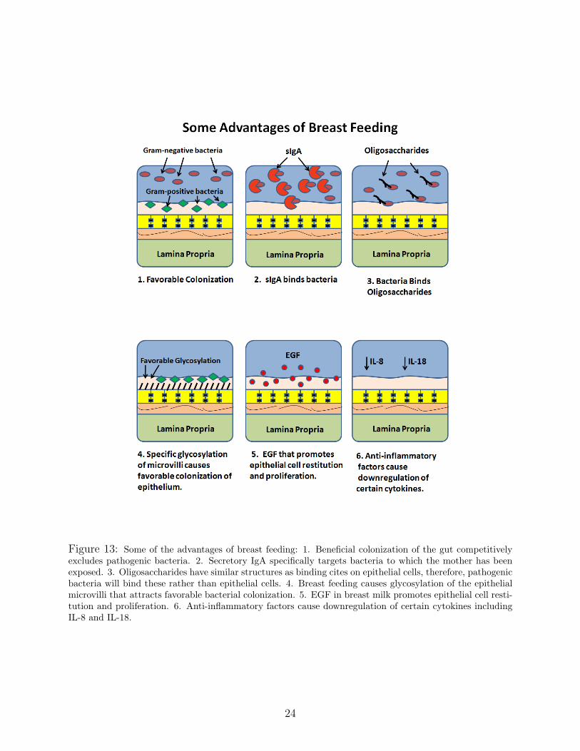
Among the advantages of breast feeding in the case of NEC are: 1) Breast feeding results
23
Figure 13: Some of the advantages of breast feeding: 1. Beneficial colonization of the gut competitivelyexcludes pathogenic bacteria. 2. Secretory IgA specifically targets bacteria to which the mother has beenexposed. 3. Oligosaccharides have similar structures as binding cites on epithelial cells, therefore, pathogenicbacteria will bind these rather than epithelial cells. 4. Breast feeding causes glycosylation of the epithelialmicrovilli that attracts favorable bacterial colonization. 5. EGF in breast milk promotes epithelial cell resti-tution and proliferation. 6. Anti-inflammatory factors cause downregulation of certain cytokines includingIL-8 and IL-18.
24
in a more beneficial colonization of the gut (that is, the gut is colonized with primarily
gram-positive bacteria) and, thereby, ”competitively excludes” more harmful pathogen from
accumulating near the epithelium. 2) There are anti-inflammatory factors in breast milk. 3)
Antibodies in breast milk such as secretory IgA bind specific pathogens to which the mother
has been exposed. 4) Oligosaccharides in breast milk act as decoys - bacteria binds to the
oligosaccharides rather than to the epithelial cells. 5) Breast milk facilitates maturation
of the intestinal mucosal barrier and 6) Breast feeding results in favorable glycosylation
patterns on the intestinal microvilli.
1. Beneficial bacterial colonization of the GI tract. Current opinion suggests that
the gram-positive bacteria bifidobacteria and lactobacilli are the most beneficial bacteria that
can colonize the infant gut. On the other hand, staphylococci and clostridia are potentially
pathogenic. [111] Breast feeding results, primarily, in gram-positive colonization of the GI
tract (e.g colonization primarily bifidobacterium, along with some lactobacillus, streptococ-
cus. In particular, lactoferrin and α-lactalbumin in breast milk stimulate the growth of
bifidobacterium [17]). Even though some enterobacteria (gram-negative bacteria) is present
in breast-fed infants, it is the bifidobacterium that predominates the breastfed infant gut
[102], [51]. Gram-positive bacteria tends to attenuate the growth of gram-negative bacteria
and leads to the production of lactic acid which is easily absorbed in the small intestine
[83],[112]. Just as importantly, gram-positive bacteria competes with pathogenic bacteria
for binding sites and nutrients.
While it is true that there is some gram-positive lactobacilli in the gut of formula-
fed infants, there are sufficient pathogenic species such as staphylococcus, escherichia coli,
and clostridia to be a potential danger [26], [51]. In general, formula feeding may lead to
proliferation of gram-negative bacteria (e.g. coliforms) in the intestine [13]. Gram-negative
colonization of the GI tract will intensify any inflammatory cascade and will make the host
vulnerable should any insult to the intestine occur. Also, gram-negative bacteria can lead to
the production of hydrogen, carbon dioxide, and organic acids. All of which are not easily
expelled from the body [112].
Infants delivered vaginally and born at home have the most beneficial gut colonization
(the most bifidobacteria and the least C. difficile and E. Coli).Hospitalization and prematu-
25
rity are both associated with C. difficile. [111] Antibiotics reduced both bifidobacteria and
bacteroides [111].
2. Anti-inflammatory factors in human milk. Goldman [45] lists several anti-
inflammatory factors in human milk: cytoprotectives, epithelial growth factors, matura-
tional factors, binders of enzymes, modulators of leukocytes, antioxidants. Also, TGF-β1 is
in human breast milk. Human milk suppresses IL-1β induced IL-8 production in intestinal
epithelial cells [100].
3. Antibodies in breast milk. Among the most important components of human
milk that serve as antimicrobial agents include IgA, lactoferrin, and lysozyme [26].
Antibodies in breast milk such as Polymeric IgA (pIgA) and secretory IgA bind anti-
gens, bacteria and endotoxin. In infants, this secretory IgA binds to pathogens before the
pathogens attach to the epithelial lining of the intestinal wall [6]. Polymeric IgA and secre-
tory IgA are produced by the mother’s immune system and are created to bind the specific
pathogens to which the mother has been exposed [26], [102]. It is likely that mother and
infant will be exposed to many of the same pathogens, therefore, these antibodies provide a
particularly relevant and valuable defensive tool.
Kohler, et. al. [72] report that human milk is rich in immunoglobulins of which about
90% is secretory IgA. The Kohler study showed that IgA concentrations in the feces of
breast-fed infants was three times high than in formula-fed infants.
Lactoferrin and lysozyme are nonspecific anti-microbial factors. [26] Lactoferrin has been
shown to have anti-microbial activities against a broad range of bacteria but all the types of
bacteria and all the conditions under which it is effective have not yet been fully established
[39], [102]. Lactoferrin also appears to work synergistically with lysozyme against bacteria
[39].
Finally, Goldman [45] notes that these antimicrobial peptides have further advantages:
they are resistant to digestive enzymes and they operate without causing an inflammatory
response.
Defensins are endogenous antimicrobial peptides produced by the epithelial surface,
26
which provide nonspecific defense against against a multitude of microorganisms. In the
small intestine, α−defensins are expressed predominantly by Paneth cells.
4. Oligosaccharides in breast milk act as decoys Human milk oligosaccharides
are complex carbohydrate structures that are normally attached to lactose and which sur-
vive the passage through the intestine [102]. Oligosaccharides actually bind to bacteria be-
fore the bacteria are able to attach to glycoconjugates on the microvillous membrane [102].
Oligosaccharides act as decoys (homologues of of host surface glycoconjugates) so that bac-
teria bind to the Oligosaccharides rather than to the glycoconjugates on the microvillus
membrane. Pathogenic bacteria will bind intestinal epithelial cells via protein adhesions but
many oligosaccharides in human milk have the same sugar sequences as the carbohydrate
chains of glycolipids and glycoproteins on human epithelial cell surfaces [34]. Thus they
prevent binding of pathogen to the intestinal epithelial cells. [26] [102], (Goldman 1993).
Oligosaccharides may also act as nutrients for beneficial commensal bacteria [100], [99].
5. Breast Milk Facilitates Maturation of Intestinal Mucosal Barrier EGF is
found in large amounts in the breast milk of the mothers of preterm infants (actually it
is found in colostrum - milk generated just before giving birth). In fact, the more pre-
mature the infant, the higher the level of EGF in breast milk [137]. Not only does EGF
promote epithelial cell restitution and proliferation but also downregulates the production
of the inflammatory cytokine IL-18 and upregulates the anti-inflammatory cytokine IL-10
[137]. Another study showed that HB-EGF, a member of the EGF family, promoted cell
migration/proliferation and resulted in reduced epithelial cell necrosis/apoptosis as well as
lower levels of Nitric Oxide [40]. Thus, EGF is particularly important to help prevent and/or
relieve NEC.
6. Favorable Glycosylation Patterns As noted above, bacteria binds to the microvilli
on the apical side of the epithelial cells. Of course, it is desirable for non-pathogenic bacteria
to bing to these cells. According to Bernt [17], certain bacteria will bind to specific glyco-
conjugate compositions on the microvilli of cells. Specific hormones in breast milk, cortisol
in particular, induces glycosylation patterns on the microvilli that results in colonization by
non-pathogenic bacteria [17]. Thus, breast feeding results in favorable glycosylation.
27
7. PAF-degrading enzyme PAF-acetylhydrolase (PAF-AH) As noted above,
the newborn has low circulating activity of PAF-AH and evidence suggest that even lower
quantities of PAF-AH are found in the pre-term infant [93]. Formula does not contain PAF-
AH but human milk contains large quantities of PAF-AH. Interestingly, studies indicate that
milk from mothers of pre-term infants contain significantly higher amounts of PAF-AH than
even normal breast milk [121], [93].
1.5.3 Particular Advantages of Breast Feeding in case of Prematurity
When one carefully considers the facts given in the last two sections, it is impossible not to
notice that for many of the disadvantages of prematurity, there is a corresponding advantage
in breastfeeding. For some reason, this fact does not appear to be emphasized in the journal
articles. Perhaps because it is so obvious? In any case, this is summarized in the following
table.
1.6 DESCRIPTION OF INFLAMMATORY CELLS, CYTOKINES, AND
OTHER FACTORS IN NEC
Macrophages. Macrophages reside in the blood stream, epithelial layer, and tissue. These
large and powerful phagocytes play a variety of roles. They are antigen presenting cells, they
secrete cytokines, they rid the body of dead cells and they ingest pathogens. Macrophages
live approximately two to four months [81].
Upon contact with bacterial LPS, macrophages release pro-inflammatory cytokines and
Nitric Oxide which can cause destruction to the tight junction protein that seals the para
cellular space between epithelial cells. Whenever (resting) macrophages come in contact with
cytokines, cytokines bind to the receptors on macrophages to cytokine-receptor complexes.
These complexes are then internalized into the macrophages. [12]
Neutrophils. Neutrophils reside in the blood stream until activated. After activation,
28
Effects of Prematurity Corresponding Advantage
of Breastfeeding
Immature glycosylation Favorable glycosylation patterns
Low levels of IgA production pIgA and sIgA in breast milk
Lower levels of Antimicrobial Antimicrobial peptides
peptides in breast milk
EGF is found in large
Low levels of EGF amounts in breast milk of mothers
of preterm infants
Elevated levels of PAF PAF-AH is found in large
Low levels of PAF-AH amounts in breast milk of mothers
of preterm infants
Excessive Immune Antimicrobial factors in
response breast milk
Table 1: Affects of prematurity and the corresponding advantages of breast feeding.
29
they move to the site of injury/insult through the blood vessels and through tissue. Neu-
trophils tend to accumulate in the tissue below the epithelium during inflammation [19].
After arriving at the site of injury/insult, the neutrophils phagocyte the pathogens and they
aid in sterilizing the wound. Unlike macrophages, neutrophils have a short life, one or two
days [81], [19].
Neutrophils can have very positive effects on wound healing such as producing IL-1β
which promotes epithelial repair. On the other hand, if the neutrophils do not encounter
pathogen in a timely manner, they cause tissue damage, in particular they may damage the
extra cellular matrix and they may release elastase which causes epithelial cell death and
permanent damage to the tight junctions. Furthermore, they may cross from the tissue side
of the epithelium to the lumenal side and in the process cause damage to the epithelium
barrier function by increasing the paracellular space. The larger paracellular space makes it
easier for toxins to cross the epithelium into the underlying tissue [19].
IL-1. This inflammatory cytokine is released by macrophages. There are two distinct IL-
1 genes: IL-1 α and IL-1 β. IL-1 α promotes the inflammatory response. It has been shown
that there is a high correlation between IL-1 synthesis and tissue damage and inflammation.
In particular, IL-1 α levels in the tissue have been correlated with intestinal necrosis [27].
These findings have been corroborated by studies that have shown significant reduction of
inflammatory cell infiltration after the introduction of IL-1ra [27]. (The description of IL-
1ra may be found below.) IL-1 helps to promote the inflammatory cascade by stimulating
other cells to produce cytokines. [33]. IL-1 β contributes to the production of nitric oxide.
In particular, it has been shown that exposing epithelial cells to TNF-α, in combination
with IFN-γ and IL-1 β, leads to increased expression of nitric oxide [53]. Increased levels of
Nitric Oxide leads to increased epithelial layer permeability (see below). IL-1 β stimulates
the production of IL-8 which, in turn, causes neutrophils to congregate near the site of the
inflammation [33], [90]. Interestingly, there is some evidence that IL-1 β may have a positive,
protective effect on intestinal mucosa integrity by stimulating the increase of Glial cells which
are critical to intestinal gut integrity [83].
IL-1ra. Interleukin-1 receptor antagonist binds to the same cell receptors as IL-1 and
thereby prevents IL-1 from binding to these sites. Upon binding, IL-1ra produces no biolog-
30
ical response. Thus, IL-ra has the effect of dampening the inflammatory cascade.
IL-4. This is an anti-inflammatory cytokine. IL-4 serves to dampen the inflammatory
cascade. It is produced by TH2 cells as well as by bone marrow stroma [83]. IL-4 has been
found to inhibit human macrophage colony formation [83] [66], IL-4 also inhibits monocyte-
derived hydrogen peroxide production [83] and the release of certain inflammatory mediators
such as TNF-α and IL-1β. It also reduces the tissue destruction caused by oxygen radicals
associated with ischemia and reperfusion injury [83]. IL-4/IL-13 have been shown to inhibit
macrophages’ ability to phagocyte pathogens [87], [132].
IL-6. IL-6 is produced by T cells, B cells, monocytes, fibroblasts, endothelial cells as
well as many other cell types [69]. Studies have found that intestinal epithelial cells, as well,
make IL-6 [124]. The release of IL-6 is stimulated by IL-1 and TNF-α as well as by other
pro-inflammatory cytokines [83]. IL-6 stimulates B cell growth [42]. There are indications
that IL-6 may play a dual role in NEC as studies show that it has both inflammatory and
anti-inflammatory effects. The inflammatory effects of IL-6 are well know. High levels of IL-6
have been shown to be associated with NEC severity [83]. Harris showed that IL-6 levels were
significantly higher in nonsurvivors compared to survivors of NEC [57]. On the other hand,
IL-6 appears to have certain anti-inflammatory affects. IL-6 can drive TGF-β activation.
Some research indicates that IL-6 may be responsible for increased local and circulating IL-
1ra, increased production of tissue inhibitors of metalloproteinases (TIMPs), and has been
shown to inhibit the production of superoxides [83]. As noted above, any up-regulation of
IL-1ra competes for the same binding cites as IL-1 but with no inflammatory effects. The
increased production of TIMPs results in the inhibition of the enzymes that degrade the
extra cellular matrix (see discussion of MMPs below). Finally, superoxides produce tissue
damage and, therefore, any inhibition thereof will help protect the host.
IL-8. IL-8 plays a major role in inflammation. IL-8 is a chemokine (a chemokine is a
special type of cytokine that is involved in cell migration) produced by enterocytes that causes
neutrophils to congregate near the site of inflammation [33], [90], [80]. For example, it has
been shown that in the midst of inflammatory cascades, the administration of neutralizing
antibodies against IL-8 resulted in reduced neutrophil infiltration and prevented neutrophil-
related tissue damage [56]. Studies have shown that, in general, IL-1β induces the production
31
of IL-8 [33], [90]. Other studies indicate that both IL-1β and endotoxin induce the production
of IL-8. [96]. For example, some studies have shown that, in the presence of TNF-α and LPS,
the inhibition of IL-1 does not fully eliminate the production of IL-8 and neutrophils leading
to speculation that TNF-α and LPS, even without the help of IL-1, may lead directly to the
production of IL-8 and neutrophils [56]. In summary, for the case of intestinal epithelial cells
(IEC’s), both IL-1β and endotoxin may lead to the secretion of IL-8. However, it appears
that IL-1β is far more effective than endotoxin in inducing IL-8 secretion by the IECs in
both pre-term and full-term infants [90],[96]. Since the IECs are prominent in the study of
NEC, IL-1β activation of IL-8 warrants a few more comments.
Studies have shown that IL-1β activation of IL-8 occurs through activation of nuclear
factor (NF-κ B). Studies by Claud, et. al. [25],[26] indicate that IL-1β activation of IL-8 is
muted by various factors found in breast milk [25]. In particular, it has been shown these
factors (e.g. TGF-β1, Epo) in breast milk inhibit the activation of NF-κ and, thereby, results
in reduced secretion by IECs [90], [25].
As a side note, one of the studies by Claud [25] indicated that the presence of the anti-
inflammatory cytokine IL-10 did not inhibit TNFα or IL-1β secretion of IL-8 by IECs. This
surprising result conflicted with the expected affects IL-10. However, the authors noted the
other anti-inflammatory features of IL-10 may result in reduced inflammation by affecting
macrophages and speculate that IL-10 may even affect IECs in an indirect way. (This same
study by Claud produced another unexpected result - EGF appears to increase secretion
of IL-8 by IECs. The authors of the report observed that pretreating IECs with EGF and,
afterwards, stimulating the cells with TNFα resulted in increased secretion of IL-8 by IECs.
This phenomenon cannot be fully explained at the present time.)
Finally, the presence of high concentrations of IL-8 is a significant indicator of the severity
of NEC. For example, studies have shown that within the first day of the onset of the disease,
IL-8 concentrations are significantly higher in infants with stage 3 NEC compared to infants
with stage 2 NEC [36].
IL-10. This is an anti-inflammatory cytokine that is produced by TH2 cells, B cells,
and monocytes [117]. Like IL-4, this cytokine serves to dampen the inflammatory response.
It has been shown that the addition of IL-10 suppressed inducible nitric oxide synthase
32
(iNOS), messenger RNA (mRNA), and nitric oxide expression in the small bowel, liver, and
serum by 60%, 89%, and 11%, respectively (Markel [83] quoting Kling [70]). IL-10 decreases
production of IL-2 [125]. It inhibits the activation of macrophages, TNF-α, IL-1β, IL-6,
and IL-8. It was discovered that IL-10 decreases the production of metalloproteinases (by
inhibiting T cell activation at its earliest stages.) [110]. It inhibits the synthesis of the
cytokines IL1, IL-6, IL-8, IL-10, and IL-12 [55]. Furthermore, IL-10 is a good indicator of
the severity of NEC, as concentrations of this cytokine were observed to be much higher
in infants with stage 3 NEC compared with stage 2 NEC. One study has shown that these
differences in concentrations between the stages continued until 72 hours after the onset of
the disease [36].
IL-12. This pro-inflammatory cytokine is secreted by B cells and macrophages and
induces the release of small amounts of IFN-γ from T cells and natural killer (NK) cells.
IL-12 is able, by itself, to stimulate the production of IFN-γ. However, in collaboration
with IFN-γ-Inducing Factor (IGIF) causes T cells to produce significantly greater amounts
of IFN-γ [2]. This appears to be due to the fact that IL-12 causes the expression of receptor
IGIF on certain cell lines [2]. In the same way, IL-12 induces the expression of the IL-18
receptor on Th1 cells. Therefore, IL-12 in collaboration with IL-18 causes T cells to produce
exponentially large amounts of IFN-γ [24].
IL-18. This pro-inflammatory cytokine, like IL-12, induces the release of small amounts
of IFN-γ but unlike IL-12, it is secreted by macrophages and IECs. Levels of IL-18 tend to
increase in step with the increased severity of NEC. [52].
There is some speculation that IL-18 is a negative regulator of TNF-α production by
IFN-γ. IFN-γ usually induces the production of TNF-α. However, in the presence of IL-12
and IL-18, even high levels of IFN-γ failed to produce TNF-α.[24].
IL-18 in combination with IL-12 leads to the production of nitric oxide and oxygen
radicals in macrophages and neutrophils. These, in turn, have both positive and negative
effects - the radicals are toxic to the microbial pathogens but also destructive to tissue [68].
(As noted above, IL-18 and IL-12 together cause the production of IFN-γ. IFN-γ, in turn,
induces macrophages and neutrophils to produce nitric oxide and oxygen radicals.)
TNF-α This cytokine can induce other cells to release IL-1, IL-2, IL-6, and IL-8 [139].
33
Although TNF-α is released from a variety of sources, they mostly come from activated
macrophages [139]. TNF-α is not only released by macrophages but is also a major activator
of macrophages. For this study, it is particularly important that TNF-α causes macrophages
to produce proinflammatory cytokines and nitric oxide [139].
IFN-γ This cytokine is secreted from T cells and NK cells. IL-12 causes T cells to
produce IFN-γ while IL-1,IL-2, and TNF together induce NK cells to produce IFN-γ [104].
This induces NO and TNF-α production. It has been shown to cause mucosal inflammation.
It has been shown that IL-12 and IL-18 individually induce T cells to produce IFN-γ while
together induce the production of very large amounts of IFN-γ (see discussion under IL-12
above). Interestingly, mice injected with large amounts of IFN-γ without the presence of
IL-12 or IL-18 did not have pathological effects [24]. There is some speculation that NO
inhibits IFN-γ production (see discussion under NO below). It is very important to note
that IFN-γ downregulates the production of the tight junction protein ZO1 [53] [35] and
IFN-γ reduces gap junction communication [76].
Platelet Activating Factor (PAF) Platelet Activating Factor is a powerful inflamma-
tory mediator and, therefore, an important player in NEC. PAF is produced by neutrophils,
macrophages, endothelial cells, and enterocytes in response to endotoxin and hypoxia [121].
PAF leads to the activation of IL-1 β, IL-6, and IL-8 [83], [22].
Its specific role in NEC is unclear. On the one hand, patients with NEC exhibit high
levels of PAF. In rat experiments, injection with PAF leads to intestinal necrosis. Also,
other experiments on rats have shown that PAF receptor antagonist prevents injury in-
duced by hypoxia, bacteria, and TNF-α [59]. Furthermore, the PAF degrading enzyme
PAF-acetylhydrolase (PAF-AH) blocks the initiation of NEC [22]. On the other hand, PAF
without the presence of bacteria failed to cause bowel injury in rat experiments [67]. There-
fore, PAF plays a major role in NEC but appears to require bacteria to cause inflammation
and damage.
PAF activates apoptosis of intestinal epithelial cells[22].
Matrix Metalloproteinases (MMPs). These are enzymes that degrade the extra
cellular matrix which supports the intestinal epithelial cells. It has been shown that TNF-α
drives the production of the MMPs. It has also been shown that activated lamina propria
34
T cells will begin a cascade that results in the production of MMPs. On the other hand,
IL-10 will inhibit T cell activation thereby reducing the destruction of the ECM by MMPs
[110]. Tissue Inhibitor of Metalloproteinases (TIMPs) controls the local activity of MMPs
in tissues. However, if the MMP production is too high, an imbalance will result and it will
not be possible for the TIMPs to control the MMPs [109],[108].
Nitric Oxide. Nitric oxide plays a number of critical roles in NEC. Nitric Oxide is asso-
ciated with epithelial barrier dysfunction. In particular, nitric oxide reduces the functional
levels of tight junction proteins. In addition, nitric oxide impairs communication between
epithelial cells by interfering with the normal function of the gap junction proteins. Nitric
oxide is, also, involved in epithelial cell death and has been shown to lead to destruction of
the tissue that underlies the epithelial layer.
Nitric oxide is produced from nitrogen oxide synthase (NOS). There are three isoforms of
NOS. However, for our study, we are particularly interested in inducible nitric oxide synthase
(iNOS). iNOS is produced from macrophages and other inflammatory cells. For example,
TNF-α and IFN-γ stimulate macrophages to produce iNOS. Nitric oxide is then produced
by oxidation of L-arginine mediated by iNOS [84], [77].
It is very important to note that nitric oxide usually only acts locally. This is partially
due to the fact that its metabolic lifespan is, perhaps, only a few seconds [84]. Specifically,
Levy et al [77] report that its half life is .1 to 10 seconds. Thus, the effects of nitric oxide are
limited to the area near where it is produced. On the other hand, iNOS expression usually
leads to the production of large quantities of nitric oxide over an extended period of time
[77]. As a result, even though nitric oxide dies out before it moves beyond the local area, its
sustained production can have devastating effects in the area near where it is produced.
The body naturally produces some NO and, in fact, moderate amounts of NO are bene-
ficial to the epithelium - nitric oxide plays an anti-microbial role and inhibits the growth of
gram-positive bacteria. [65] [77] However, under stressed conditions, large amounts of NO
can be produced causing damage to the epithelial layer, the tight junction proteins, and the
gap junction proteins [77].
Nitric oxide is strongly linked to epithelial layer permeability. Tight junction proteins
are responsible for maintaining a barrier to pathogen attempting to pass between epithelial
35
cells into the underlying tissue layer. Nitric Oxide has been shown to reduce the functional
levels of the tight junction proteins, ZO1, ZO3, and occludin [53].
It is theorized that NO impairs phosphorylation of the gap junction protein Cx43, re-
sulting in reduced cell-to-cell communication. This communication is required for epithelial
cell migration. Therefore, NO impairs epithelial cell migration that is required for mucosal
repair [5].
Nitric Oxide also reacts with superoxide O−2 to produce the oxidant peroxynitrite
(ONOO−). Peroxynitrite inhibits the proliferation and differentiation of epithelial cells [130].
Gap Junction Proteins. These are intercellular membrane channels that facilitate the
passage of ions and solutes between adjacent cells. These membrane channels are composed
of the gap junction protein connexin 43 (Cx43). Leaphart, et al [76] have demonstrated that
epithelial cells migrate in unison and that gap junction communication plays a crucial role in
the migration of intestinal epithelial cells during intestinal healing after injury. They show
that epithelial cells, in particular IEC-6 cells, exposed to IFN-γ exhibit reduced gap junction
communication and, therefore, greatly reduced migration speed. In particular, they showed
that IFN effected this reduced communication by dephosphorylating Cx43 and by causing
Cx43 to move inside the cell. Interestingly, inhibited gap junction communication does not
appear to reduce epithelial cell proliferation nor does it appear to induce epithelial cell death
[76].
A key factor in gap junction communication is the phosphorylation and surface local-
ization of the gap junction protein Cx43. Any inhibition of phosphorylation of Cx43 will
lead to an inhibition of epithelial cell migration. Anand, et al [5] has demonstrated that
macrophage activation leads to production of nitric oxide. The nitric oxide, in turn, inhibits
the phosphorylation of Cx43 resulting in significantly reduced cell migration.
Tight Junction Proteins.(Zonula Occludens) These include occludin, ZO-1,ZO-2, ZO-
3, claudin-1, and JAM. [74]. These proteins are formed between adjacent epithelial cells and
are closely linked with the actin-based cytoskeleton [53]. Among other functions, Zonula
Occludens serve as a barrier to keep bacteria and other molecules from passing through the
36
epithelial layer into the underlying tissue. It has been discovered that tight junctions restrict
passage of molecules based on the size of the particles and, in fact, the size of the solutes
that are allowed to pass between cells varies at different locations in the intestine. In partic-
ular, the permeability to larger solutes decreases from the crypt to the villus [128]. Also, by
restricting transport across the epithelium, the tight junctions serve to prevent equilibrium
across on both sides of the epithelium. In this way, a concentration gradient is maintained
across the epithelium. This concentration gradient is needed in order that the epithelium
can properly absorb and secrete substances [128].
Many factors effect the integrity and health of the tight junction proteins. For example,
there is a close connection between the presence of nitric oxide and increased epithelial layer
permeability. It is theorized that nitric oxide alters the expression and localization of some of
the tight junction proteins, in particular ZO1 [53]. Furthermore, it has been discovered that
IFN-γ causes a time-dependent down-regulation of the tight junction protein ZO1 [35], pg.
23. Some studies also indicate that TNF causes increased paracellular permeability [128].
Therefore, TNF may effect the tight junction protein.
DAMPs and Damaged cells. Injured cells send out danger/alarm signals. Cells
that send out such signals are cells that are exposed to bacteria, toxins, or cells that have
sustained mechanical damage. This is particularly true of cells that are in the process of
dying after an insult or injury. [88] Alarm signals might be in the form of any substance made
or modified by the dying cell. Cells that die under a normal process will not send out these
danger signals. [88] These alarm/danger signals are known as Damage-associated Molecular
Pattern molecules [DAMPs]. DAMPs tend to keep inflammation going even when most or
all of the invading bacteria has been killed. Therefore, a cycle of damage - inflammation -
damage can occur. [134]
LPS. LPS is a glycolipid on the outer membrane of gram-negative bacteria which com-
bines with other components and forms LPS/CD-14 [71], [126], LPS/CD-14 is recognized by
and becomes attached to TLR4.
The LPS/CD-14 complex leads to secretion of IL-1, IL-6, and TNF-α in macrophages
[89].
TLR4. TLR4 is one member of the group of Toll-like receptors. Also referred to as
37
pattern recognition molecules (PRMs) or pattern recognition receptors (PRRs). Toll-like re-
ceptors are normally expressed on the outside of the cell on what is known as the cell mem-
brane or plasma membrane and they recognize large molecules that are associated with
pathogens. These large molecules are sometimes referred to as pathogen-associated molecu-
lar patterns (PAMPs) or microorganism-associated molecular patterns (MAMPS) [55]. For
our study, the only toll-like receptors that we need to consider are TLR4 and TLR9. TLR4
recognizes lipopolysaccharide (LPS) which is on the outer membrane of gram-negative bac-
teria. TLR4 is expressed on many different types of cells. However, we are most interested
in TLR4’s role on intestinal epithelial cells (IECs).
It has been discovered that TLR4 mediates phagocytosis of gram-negative bacteria by
IECs. This results in IECs translocating bacteria from the mucosa to underneath the ep-
ithelial layer in a transcellular manner [97].
On IECs, TLR4-LPS binding begins a signalling cascade inside the cell ultimately result-
ing in integrin activation. Often TLR4-LPS binding results in over-expression of integrins
resulting in reduced cell motility. Other adverse affects of TLR4-LPS binding are increased
epithelial cell apoptosis, inhibited cell-cell communication, and decreased cell proliferation
[41],[75]. Not surprisingly, there appears to be a strong correlation high levels of TLR4
expression and NEC severity [50]. In particular, high levels of TLR4 have been associated
with a decrease in goblet cells and, in turn, a reduction in the protective mucins that goblet
cells produce [123].
It has been observed that TLR4 increases during gut development. Fold expression of
TLR4 in the gut in mice was shown to increase approximately three-fold from embryonic
day 14 to day 18. Then goes back to day 14 levels right after birth. TLR4 expression then
increases but falls again after weaning [46],[122].
In humans, at the time of full-term birth, TLR4 expression drops greatly. On the other
hand, TLR4 expression remains high at the birth of the pre-term infant and continues to
remain high after birth (yet another disadvantage of prematurity) [50].
There are indications that Heat Shock Protein-70 (HsP70) regulates TLR4 signalling
resulting in decreased NEC severity [1].
TLR9. TLR9, like TLR4 is a Toll-like receptor. TLR9 is the receptor for bacterial
38
Figure 14: Results of TLR4 signalling.
DNA (CpG-DNA). It has been determined that TLR4 and TLR9 have a reciprocal role,
i.e., increased signalling in one TLR is associated with decreased signalling of the other.
Studies have shown that, in enterocytes, activating TLR9 with CpG-DNA inhibited LPS-
mediated signalling by TLR4 [46]. Furthermore, NEC has been found to develop in a mucosal
environment of increased TLR4 expression and decreased TLR9 expression [46].
Integrins. Integrins are cell surface glycoproteins that are responsible for cell adhesion
to the extra cellular matrix on which the epithelium resides. Proper integrin expression is
critical for proper cell migration after an injury. Signals from inside the cell cause integrins to
become activated. Upon TLR4-LPS binding, a signalling cascade begins resulting in integrin
activation.
Extracellular ligands of integrins are primarily proteins of the ECM such as fibronectin
and collagen. As a result of this binding to proteins of the ECM, the integrins form clusters
known as focal adhesions [73]. Integrins then transmit signals across the plasma membrane
and, in cooperation with growth-factor initiated signals determine various cell functions [9],
[63].
This concludes the survey of the medical research of NEC. The topics in this chapter
were presented as they relate to NEC. More general information about these topics may
be found in other sources. Janeway’s Immunobiology [95] provides a good introduction to
the immune system. For cell signalling, see Marks, Klingmuller, and K. Muller-Decker [84].
39
2.0 PREPARATIONS FOR CONSTRUCTION OF A NEC MODEL
Much information related to NEC was presented in the previous chapter. In that chapter,
many of the mechanisms and factors involved in NEC were explored and examined. Most
of that information will now be organized, summarized, and filtered down into a form that
can be used for a 3-D mathematical NEC model. Some of the material in that first chapter
will not be used in a direct way to construct the NEC model but will be used to inform the
simulation runs later in the thesis. For example, when simulating prematurity in chapter
seven, underdeveloped peristalsis, which is a common problem for the pre-term infant, will
be simulated by including large amounts of bacteria near the epithelium. On the other hand,
some factors presented in chapter one that have common characteristics will be combined
into single factors for the purpose of the model. For example, the cytokines that have
inflammatory effects will be combined into the general category of cytokines. In addition,
certain practical considerations must be kept in mind when constructing this model. This is
the first 3-D model for NEC, it will be wise not to include too much detail in this first model.
Also, there is currently very little quantitative clinical data concerning some of the specific
NEC factors covered in chapter one. As a result, some simplification and/or combining of
NEC factors is necessary. Therefore, the main goal of this chapter will be to identify the
most essential factors in NEC, generalize these factors as much as possible, and define the
interaction among these factors. This work will result in the General Inflammatory Cascade
presented in this chapter (see figure 21). In chapter three, this General Inflammatory Cascade
will be used as a guide for the construction of the 3-D mathematical NEC model.
The General Inflammatory Cascade will be presented after the construction of interme-
diate diagrams and cascades. It is possible to construct the General Inflammatory Cascade
without these intermediate steps and diagrams. However, it is important that the reader
41
understand the rationale for many of the simplifications that will be done in this chapter.
Also, this intermediate information will provide ideas and motivation for a more advanced
NEC model in the future. That is, this intermediate information may supply the next level
of detail that can be included in a more extensive NEC model. This information will be
particularly relevant as soon as new clinical data becomes available that touches the factors
included in these intermediate steps.
2.1 INFLAMMATORY CASCADE
In this section, inflammatory cascades and other diagrams will be developed based on the
information presented in chapter 1. An inflammatory cascade which shows the interplay
between cytokines, bacteria, etc. is presented in figure 15. (This cascade is a generalization
based on the information presented in chapter 1.) In order to preserve clarity, PAF and its
role in the inflammatory cascade is not included in figure 15 but in a separate figure (figure
16). In figure 15 we have the following important information (this is all based on the
material presented in chapter 1):
1) Beginning along the bottom of the diagram, macrophages eliminate bacteria. At
the same time, bacterial contact with macrophages induces the production of IL-12,IL-18,
TNF-α.
2) TNF-α induces the production of IL-1, IL-2, IL-6, and IL-8. TNF-α in combination
with IL-1, IL-2 induce NK cells to produce IFN-γ (this combination is indicated by the blue
++.) TNF-α also induces the production of MMPs.
3) IL-12 and IL-18 individually induce the production of IFN-γ but in combination IL-12
and IL-18 produce even larger amounts of IFN-γ (this combination is indicated by the blue
++.)
4) IL-18 induces the production of IL-4,5,8,10,13.
5) Both IL-1 and TNF-α induce the production of IL-6.
6) IL-6 induces the production of IL-1ra and TIMPs. IL-1ra in turn reduces the effects
of IL-1 by competing for the same binding sites as that cytokine. (IL-6 also leads to TGF-β
42
Figure 15: Partial Inflammatory Cascade. See the text for discussion. Symbols: Ma stands for activatedmacrophages, Na for activated neutrophils, B for bacteria, the other symbols are self-explanatory. Boxcolor designations are as follows: inflammatory cytokines and other destructive agents have whitebackground boxes; cytokines and other factors that play an anti-inflammatory role have green backgroundboxes; phagocytes have yellow background boxes; free radicals have boxes with gray background. Arrowcolor designations are as follows: a red arrow with a negative sign indicates downregulation or productioninhibition; a black arrow with a positive sign indicates upregulation; whenever two or more arrows meet at aplus sign with a blue background, this indicates that two or more factors, when working together, induce theproduction of a large amount of a substance. Note that activated neutrophils, like activated macrophages,produce cytokines and nitric oxide. For clarity, this function of activated neutrophils is not shown in thefigure. Note, also, that some of the intermediate roles of the inflammatory cells are not shown here. Forexample, the diagram implies that TNF-α and IFN-γ directly produce nitric oxide and O2- but in realityTNF-α and IFN-γ induce macrophages to produce these molecules. Also, IL-10 does not directly inhibit theproduction of MMP’s. Instead, IL-10 inhibits the T cell activation which, in turn, slows the production ofMMP’s. Finally, the function of IL-4, IL-8, and IL-10 are shown near the middle of the diagram but theproduction of these cytokines is shown in the upper left hand corner.
43
Figure 17: Disruption and restoration of the epithelium. This diagram, unlike the inflammatory cascades,shows the physical effects on the structure of the epithelium. At the top of the illustration we see that nitricoxide destroys gap junction protein (GJP), epithelial cells and tight junction protein(TJP). Also, ONOO-destroys epithelial cells and IFN-γ downregulates the production of tight junction protein. At the bottom,we see that nitric oxide, IFN-γ, and ONOO- inhibits epithelial restitution. Paradoxically, IFN-γ promotesepithelial cell migration and, therefore, also contributes to epithelial restitution.
45
Figure 18: Other factors involved in epithelial restitution/proliferation. Epithelial cells produce TGF-α;Lamina propria cells produce TGF-β; Salivary glands produce EGF; Goblet cells produce TFF. TGF-β,EGF, and TFF all enhance epithelial cell migration. TGF-α and EGF enhance epithelial cell proliferationbut TGF-β inhibits epithelial cell proliferation.
46
activation.)
7) TIMPs inhibit the production of MMPs.
8) IL-1β induces the production of IL-8.
9) IL-8 causes neutrophils to congregate near the site of inflammation.
10) IL-10 inhibits production of TNF-α, IL-1β, IL-6, and IL-8.
11) Not shown is the fact that IL-10 may inhibit MMP production by inhibiting T cell
activation.
12) On the bottom right of the diagram, TNF-α and IFN-γ causes macrophages to
produce Nitric Oxide and O−2 .
13) Also on the bottom right of the diagram, Nitric Oxide reacts with O−2 to produce
ONOO−.
Other effects not explicitly shown:
14) IL-4, particularly with IL-13, inhibits macrophages’ ability to phagocytize pathogen.
15) IL-4 inhibits macrophages’ ability to produce nitric oxide.
PAF’s role in the inflammatory cascade is given in figure 16. Here it is shown that activated
macrophages and activated neutrophils produce PAF. PAF, in turn, leads to the activation
of IL-1β, IL-6, and IL-8.
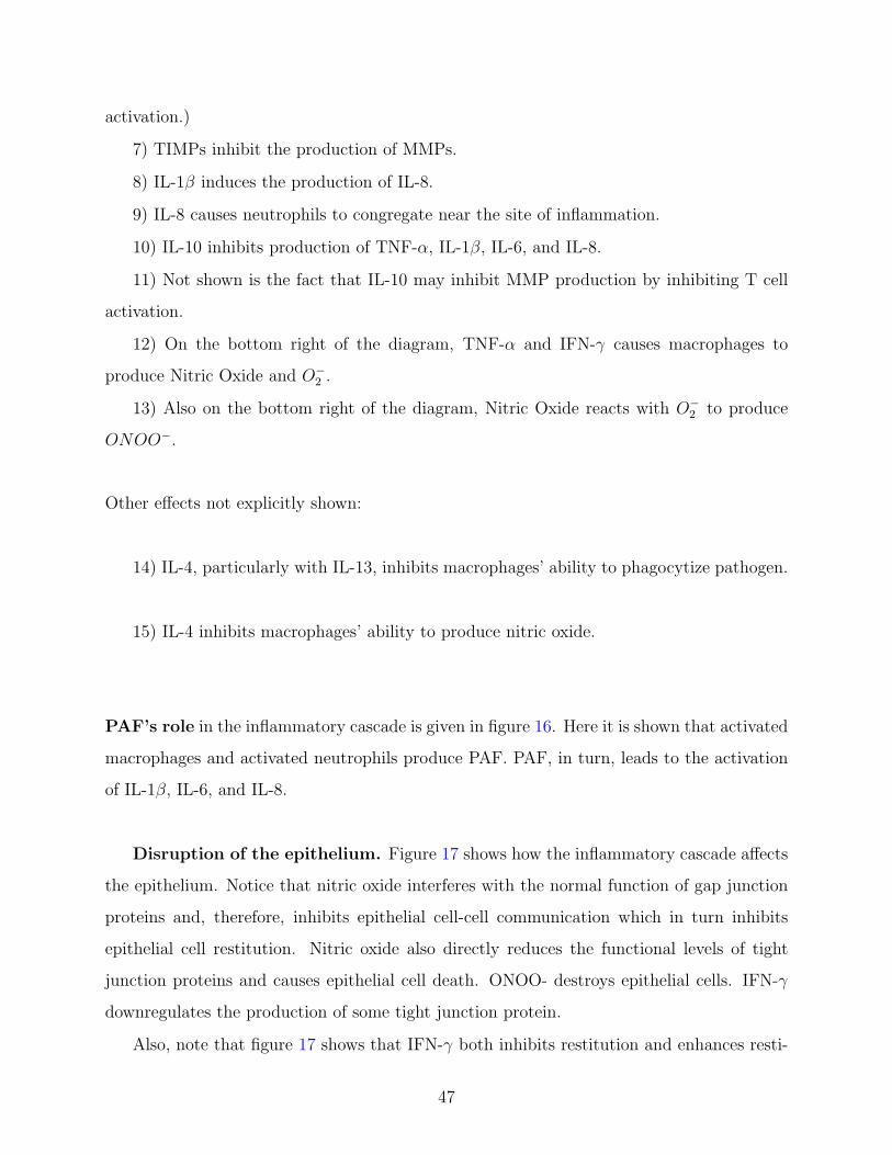
Disruption of the epithelium. Figure 17 shows how the inflammatory cascade affects
the epithelium. Notice that nitric oxide interferes with the normal function of gap junction
proteins and, therefore, inhibits epithelial cell-cell communication which in turn inhibits
epithelial cell restitution. Nitric oxide also directly reduces the functional levels of tight
junction proteins and causes epithelial cell death. ONOO- destroys epithelial cells. IFN-γ
downregulates the production of some tight junction protein.
Also, note that figure 17 shows that IFN-γ both inhibits restitution and enhances resti-
47
tution of the epithelium. This is based on the evidence, presented in chapter one, that IFN-γ
reduces gap junction communication [76] and, one would conclude, slows epithelial restitu-
tion. Other evidence, also presented in chapter one, suggests that IFN-γ promotes epithelial
cell migration [32].
Other factors involved in epithelial restitution/proliferation Figure 18 is a sim-
plification and summary of much of the information that was presented in the last chapter.
(See the discussion in chapter one and figure 10 in that chapter.) Recall from chapter one
that many of the growth factors such as HGF, and FGF peptides as well as the cytokines
IL-1, IL-2, IFN-γ affect the epithelium through TGF-β dependent pathways. Therefore, in
figure 18 the functions of these particular growth factors, peptides and cytokine are repre-
sented simply by TGF-β. On the other hand, the growth factor EGF plays such an important
role in epithelial proliferation and restitution that its explicit inclusion in figure 18 is war-
ranted. TGF-α, which is produced by epithelial cells is explicitly included for similar reasons
- it plays an important role in epithelial proliferation. Members of the trefoil factor family
(TFF), which are produce by goblet cells, work in conjunction with glycoproteins on the
apical side (lumenal side) of the epithelium through an TGF-β independent pathway (see
chapter one) and it is, therefore, explicitly included.
2.2 PHYSICAL DOMAIN FOR THE NEC MODEL.
Based on the discussion in chapter one, the lumen, the mucus, the epithelial layer, the extra
cellular matrix (ECM), the underlying tissue, and the blood (or circulatory system) are
important regions for the study of NEC. Ideally, all of these regions would be included in
the mathematical model. However, a model that includes six regions may be too complex.
So, the number of regions considered will be reduced. The mucus will not be included in
the mathematical model because it, like the epithelium, is part of the mucosa. Much of
what occurs in the mucus can be considered together with the epithelial layer. The integrity
of ECM is closely related to the integrity of the epithelium. Recall that the ECM is the
48
Figure 19: This diagram shows how the presence of nitric oxide and IFN-γ results in epithelial
layer permeability.
foundation upon which the epithelial cells stand. Any degradation of the extra cellular matrix
will contribute to epithelial layer permeability. Therefore, extra cellular matrix permeability
and epithelium permeability will not be treated as separate functions. The extra cellular
matrix will not be included in the physical domain for the mathematical model. The function
of the ECM will be included in the function of the epithelium. This leaves us with four regions
as seen in figure 20.
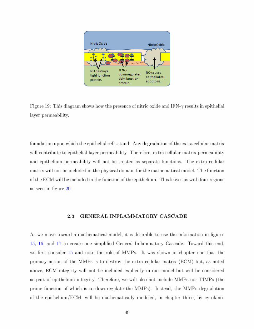
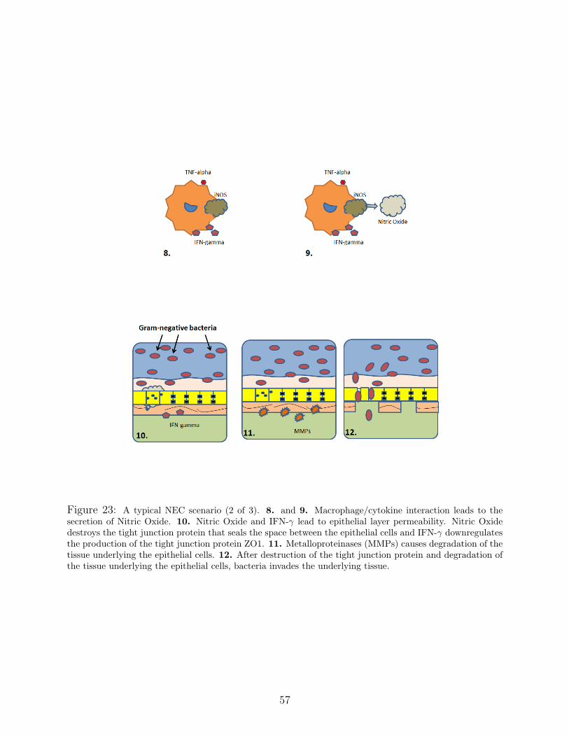
2.3 GENERAL INFLAMMATORY CASCADE
As we move toward a mathematical model, it is desirable to use the information in figures
15, 16, and 17 to create one simplified General Inflammatory Cascade. Toward this end,
we first consider 15 and note the role of MMPs. It was shown in chapter one that the
primary action of the MMPs is to destroy the extra cellular matrix (ECM) but, as noted
above, ECM integrity will not be included explicitly in our model but will be considered
as part of epithelium integrity. Therefore, we will also not include MMPs nor TIMPs (the
prime function of which is to downregulate the MMPs). Instead, the MMPs degradation
of the epithelium/ECM, will be mathematically modeled, in chapter three, by cytokines
49
Figure 20: This diagram shows the four regions that will be used in the NEC mathematical
model.
affecting epithelial layer integrity. This simplification is reasonable because the cytokine
TNF-α induces the production of MMPs as can be seen from figure 15. On the other
hand, we will include the immune cells, activated macrophages, ma, and activated
macrophages, Na, in the General Inflammatory Cascade. Next note that figures 15 and 16
indicate that activated macrophages and activated neutrophils, either directly or indirectly
induce the production of all the inflammatory cytokines. (By ”indirectly”, it is meant that
activated macrophages and activated neutrophils induce the production of some cytokines
which, in turn, induce the production of the remaining cytokines shown in the figures.) That
is, activated macrophages and activated neutrophils induce the production of TNF-α, IL-1β
IL-12, IL-18, PAF, these in-turn induce the production of IL-1,IL-2, IL-4, IL-5, IL-8, IL-10,
IL-13, IFN-γ then IL-1 induces the production of IL-6. Therefore, it will be reasonable to
group all of the aforementioned inflammatory cytokines under cytokines, c. Furthermore,
note that in figure 15 that the anti-inflammatory cytokines such as IL-4, IL-10, IL-1ra
downregulate most of the inflammatory cytokines. Therefore, these anti-inflammatory
50
cytokines, ca, may be grouped together.
Note that figure 15 indicates that the same factors that produce NO also produce O2-.
Furthermore, NO and O2- together produce ONOO-. Therefore, it is possible to include
nitric oxide, NO, in the General Inflammatory Cascade and not O2- nor ONOO- as long
as we assign the affects of O2- and ONOO- to NO. For example, note that O2- destroys
bacteria so in the General Inflammatory Cascade we will indicate that NO destroys bacteria.
Also, in figure 17 we see that ONOO- destroys epithelial cells and interferes with epithelial
layer restitution but this action mirrors the action of nitric oxide.
In figure 17 we see that nitric oxide (NO) destroys epithelial cells, tight junction protein
and gap junction protein. As noted in chapter one, gap junction protein is necessary for
epithelial cell communication and for coordinated epithelial cell migration. So, if we model
epithelial cell migration and proliferation together, we will not need to include gap junction
protein in our General Inflammatory Cascade. That is, we will assume that nitric oxide will
cause destruction of the epithelial layer and inhibit its repair.
On the other hand, it would be wise to include tight junction protein, ZO1, in the
General Inflammatory Cascade because it is possible for enough nitric oxide to be present to
destroy the tight junction protein, and therefore, create epithelial layer permeability, without
(or before) destroying epithelial cells.
In figure 17, we see that IFN-γ both helps and inhibits epithelial restitution. Based
on the evidence presented in chapter one, the net action of IFN-γ is more likely to inhibit
epithelial restitution than to promote restitution. Therefore, IFN-γ may be left out of the
general inflammatory cascade and its action represented by cytokines, which inhibit epithelial
restitution.
epithelial cells, ec, are essential to the model and, of course will be included in the
General Inflammatory Cascade. Note in figure 17 that many of the factors that contribute to
epithelial proliferation and restitution originate in the epithelium itself or originate naturally
in other parts of the body, i.e., the tissue and salivary glands. It will, therefore, be reasonable
to exclude all of the factors in figure 17 from the General Inflammatory Cascade and represent
their effects by terms in the epithelial cell equation (this last part will be done in chapter
three).
51
Damage (in the context of DAMPs) was covered in chapter one but it was not included
in figures 15, 16, or 17 because as noted in the first chapter, many different components
produced or modified by injured or dying cells can play the role of DAMPs. Therefore,
DAMPs did not fit in well with the well defined components shown in figures 15, 16, or 17.
On the other hand, DAMPs fit well into the General Inflammatory Cascade in which each
component may represent a more general class of components. Also, as noted in chapter
one, damage is a major player in keeping the inflammatory cascade going, even after all of
the bacteria has been destroyed. Therefore, it is necessary to include damage, d, in the
General Inflammatory Cascade.
Finally, bacteria, b, is essential for the model and, therefore, will be included in the
general inflammatory cascade. So, the General Inflammatory Cascade is given in figure 21.
This General Inflammatory cascade may be though of as occurring in multiple regions, with
the understanding, of course, that epithelial cells are present only in the epithelial region.
In figure 21, the components are as follows:
b: bacteria - endotoxin, LPS; Interacting with activated neutrophils and activated
macrophages, induces the production of cytokines. This effect is indicated by the black
dashed lines in the diagram. At the same time, activated neutrophils and activated
macrophages destroy bacteria. (This is indicated by the red arrows pointing from activated
neutrophils and activated macrophages toward bacteria).
c: pro-inflammatory cytokines. This group includes IL-1, IL-8, IL-12, IL-18, IFN-γ, TNF-
α and, perhaps IL-6 (although as indicated in chapter 1, IL-6 may have both inflammatory
and anti-inflammatory affects). These cytokines induce macrophages and neutrophils to
produce other cytokines (As indicated by the solid black lines going to and from activated
neutrophils and activated macrophages). Also, these cytokines induce macrophages and
neutrophils to produce nitric oxide. (This is indicated by the black dashed lines). Certain
cytokines such as TNF can induce epithelial cell death. (This is indicated by the red line
pointing from the cytokines to epithelial cells.)
ca: anti-inflammatory cytokines - This group includes IL-4 and IL-10. These cytokines
tend to reduce the inflammatory response by slowing down the production of cytokines,
activated neutrophils and activated macrophages. (This is indicated by the blue dashed
52
Figure 21: General Inflammatory Cascade. See the text for discussion. Symbols: ma stands foractivated macrophages, Na for activated neutrophils, b for bacteria, Ca for anti-inflammatory cytokines, dfor damage, NO nitric oxide, ZO1 represents tight junction protein, ec represents epithelial cells. Arrowcolor designations are as follows: a red arrow with a negative sign indicates downregulation or productioninhibition; a black arrow with a positive sign indicates upregulation.
lines in the diagram).
d: damage - Damage was covered in chapter 1 under DAMPs, Damage-associated Molec-
ular Pattern molecules. Damage might be thought of as the measure of the level of severity of
the inflammation. DAMPs are induced by inflammation in stressed/injured cells and which
serve to perpetuate inflammation in a feed-forward fashion [43], [88], [135].
ec: epithelial cells - these cells line the intestinal wall and protect the underlying tissue
from bacterial invasion. Tight junction proteins, such as ZO1, seal the space between these
cells so that pathogen may not pass into the underlying tissue [53], [54].
m: macrophage - resting immune cells. (For clarity, these are not explicitly shown in the
diagram but will be included in the PDE model developed in chapter 3.) Macrophages are
activated by bacteria, cytokines, and damage.
ma: activated macrophage - activated immune cells. These cells phagocytose bacteria.
These cells release inflammatory cytokines and nitric oxide.
n: neutrophil - resting immune cells normally found in the bloodstream. (For clarity,
53
these are not explicitly shown in the diagram but will be included in the PDE model devel-
oped in chapter 3.) Neutrophils are activated by cytokines and damage.
na: activated neutrophil - activated immune cells that move from the blood stream
toward the site of infection. These cells release inflammatory cytokines and nitric oxide.
NO: nitric oxide - this chemical is released by activated macrophages and activated
neutrophils after these inflammatory cells come in contact with certain cytokines (this is
indicated by the black dashed lines coming from activated macrophages and activated neu-
trophils to nitric oxide. Nitric Oxide destroys the tight junction protein, ZO1, that seals the
space between epithelial cells [53], [54]. (This is indicated by the red arrow from the nitric
oxide to ZO1). Finally, the presence of nitric oxide in the epithelium leads to epithelial cell
apoptosis. (This is indicated by the red arrow from the nitric oxide to the epithelial cells).
ZO1: tight junction protein - keeps the epithelial cells in close apposition and prevents
the passage of bacteria into the underlying tissue. Nitric Oxide destroys this protein.
2.4 A TYPICAL SCENARIO
At this point, it will be wise to use the information in chapter one to put together a typical
NEC scenario, that is, a sequence of events in the progression of the disease. It will be
helpful to have such a scenario available when constructing the NEC mathematical model
and when doing simulations. There are many possible cases of scenarios. The following
example is a typical case of a premature, formula fed infant with no initial injury
to the intestinal barrier. To be sure, even this case has many possible variations within
it but we will pick one variation that includes all of the features of this particular case.
Under this scenario, formula feeding causes bacterial colonization of the lumen. Un-
derdeveloped peristalsis, a common problem in the premature infant, does not clear away
the bacteria (figure 22, # 1). Some of the bacteria that lingers for a long time near the
epithelium eventually passes through the protective epithelial cells and invades the under-
lying tissue (figure 22, # 2). Note that this bacterial translocation may occur by several
54
different mechanisms (see figure 12 in chapter 1). Bacteria that gets into the underlying
tissue invokes an inflammatory response. Macrophages interacting with the bacteria become
activated. The activated macrophages release cytokines, in particular, TNF-α (figure 22, #
3 and # 4). The TNF-α causes increased production of IL-1 [16] and MMP’s [83] (figure
22, # 5). The activated macrophages also release the cytokines IL-12 and IL-18 which each
induce T and NK cells to produce IFN-γ (figure 22, # 6). Recall from chapter one that
IL-12 and IL-18 acting together cause an exponential increase in IFN-γ (figure 22, # 7).
Many of the cytokines that have been produced then act on the macrophages. In par-
ticular, TNF-α and IFN-γ cause macrophages to produce inducible Nitric Oxide synthase
(iNOS) which, in turn, produces Nitric Oxide (NO) (figure 23, # 8 and # 9).
Large amounts of nitric oxide and cytokines near the epithelium lead to its destruction.
The nitric oxide causes both the death of epithelial cells as well as destruction of the tight
junction protein, such as ZO1, which normally seals the space between the epithelial cells.
As noted in chapter one, IFN-γ causes a time-dependent down-regulation of ZO1(figure 23,
# 10). Simultaneously, MMP’s cause the degradation of the Basal Lamina that underlies the
the epithelial layer (figure 23, # 11). All of this together results in the greater permeability
of the epithelial layer.
The degraded epithelial layer provides only minimal protection for the underlying tissue.
Bacteria and other species may easily travel from the lumen into the underlying tissue (figure
23, # 12). After the bacterial invasion, the tissue becomes the location of a very aggressive
inflammatory cascade that involves, among others, IL-1, IL-6, IL-8, IL-12, IL-18, IFN-γ,
TNF-α, and HMGB1 (figure 24, # 13 and # 14).
While this is occurring, the epithelial layer attempts to repair itself. However, as noted
earlier, IFN-γ causes a significant reduction in phosphorylated Cx43, a gap junction pro-
tein critical to cell-cell communication and epithelial cell migration. Nitric Oxide similarly
prevents the phosphorylation of Cx43. Interference with gap junction proteins results in
inhibited epithelial cell migration. Furthermore, over-activation of TLR-4 by lumen bacteria
results in over-expression of integrins. Too much integrin expression results in the epithelial
cells adhering too tightly to extra-cellular matrix (see chapter one). All of this results in
greatly reduced cell migration and in a sustained wound (figure 24, # 15).
55
Figure 22: A typical NEC scenario (1 of 3). 1. Gram-negative bacterial colonization near the epithelium.2. Bacteria pass through the epithelium and invades the underlying tissue. 3. Bacteria in the lumen comesin contact with macrophages. 4. The macrophages respond by releasing cytokines such as TNF-α. 5. TNF-α increases production of Metalloproteinases (MMPs) and induces the release of cytokines such as IL-1 . 6.Macrophages also release other cytokines such as IL-12 and IL-18. IL-12 and IL-18 each provoke the releaseof IFN-γ. 7. IL-12 and IL-18 work together to induce the release of large amounts IFN-γ.
56
Figure 23: A typical NEC scenario (2 of 3). 8. and 9. Macrophage/cytokine interaction leads to thesecretion of Nitric Oxide. 10. Nitric Oxide and IFN-γ lead to epithelial layer permeability. Nitric Oxidedestroys the tight junction protein that seals the space between the epithelial cells and IFN-γ downregulatesthe production of the tight junction protein ZO1. 11. Metalloproteinases (MMPs) causes degradation of thetissue underlying the epithelial cells. 12. After destruction of the tight junction protein and degradation ofthe tissue underlying the epithelial cells, bacteria invades the underlying tissue.
57
Figure 24: A typical NEC scenario (3 of 3). 13. and 14. Bacteria in the tissue results in an aggressiveinflammatory response resulting in the release of cytokines such as IL-1, IL-6, IL-8, IL-12, IL-18, IFN-γ,TNF-α, HMGB1. 15. Nitric oxide and IFN-γ interferes with gap junction proteins. Bacteria contact withthe epithelial cells leads to over expression of integrins. All of this leads to reduced epithelial migration. 16.Macrophages produce nitric oxide and O2 radicals which, in turn, produce ONOO-. 17. The NO/ONOO-/O2 Radicals Cause Epithelial Cell Death/Tissue Death.
58
The inflammatory cascade is now unchecked. The production of nitric oxide and O2
radicals leads to the production of ONOO−. [130](figure 24, # 16). These work together
to cause extensive tissue death (figure 24, # 17). The ultimate result will be organ failure
and possibly death to the infant.
In this chapter, much of the material from chapter one has been organized, summarized,
and put into a form that may now be used to construct a NEC model. In particular, the
General Inflammatory Cascade (see figure 21) has been constructed. This General Inflam-
matory Cascade, which shows the interaction among the major players in NEC, will provide
the basis for the NEC mathematical model. This cascade can be converted directly into a
basic mathematical model. Other information presented in the present chapter will be used
to add greater detail to the model. The NEC mathematical model will be constructed in
the next chapter.
59
3.0 A PARTIAL DIFFERENTIAL EQUATION MODEL FOR NEC
This chapter presents a three dimensional mathematical model for NEC. The General In-
flammatory Cascade developed in chapter two (see figure 21), will be used as a blueprint for
the mathematical model. Other information presented in chapters one and two will be used
to create detail in the model.
Mathematical models for NEC and/or inflammation have been developed in the past
[116], [29], [8], [129]. These models are extremely valuable and provide important insights
into the disease. Furthermore, many of the parameters, mathematical terms, and functions
developed in these papers will continue to be used in future NEC mathematical models. In
fact, a number of terms developed in Reynold.s et al. [116] that model inflammation will be
used in the 3-D mathematical model developed in this chapter. (These will be noted below.)
However, the models mentioned above are all one dimensional, ordinary differential equa-
tion (ODE) models and, therefore, simulate only the transient effects of NEC but do not fully
model its spatial effects. Only a 3-D model can accurately simulate diffusion and advection
of the major players in NEC, account for the different effects of NEC in the different regions
in the body (as noted in chapter two, our mathematical model will include four different
regions, see figure 20), and fully integrate all the effects of epithelial cell degradation and
migration. Therefore, a 3-D model will fill a void in the NEC mathematical models.
Before going forward, it is important to note that several people, over a period of sev-
eral years, contributed to the development of the NEC PDE system presented in this chapter:
Joshua Sullivan, Ivan Yotov, Mark Tronzo, Christopher Horvat, Jared Barber, Yoram
Vodovotz, Jeff Upperman, Gilles Clermont.
60
The author of this thesis will, here, present the PDE system and attempt to give justifi-
cation for the structure of each equation. In the process, the close connections between the
PDEs and the data presented in chapters one and two will be noted.
3.1 DERIVATION OF PARTIAL DIFFERENTIAL EQUATIONS
In this section, the partial differential equations for the NEC model will be constructed using
the General Inflammatory Cascade, figure 21, as a guide.
Activated macrophages. Activated Macrophages will diffuse in the direction of de-
creasing density of activated macrophages. Thus the activated macrophage equation will
have a diffusion term, ∇ · (−Dma∇ma). Activated macrophages will move in the direction
of increasing cytokines and increasing bacteria. So, the advection term may be written as
∇ · (γmacma∇c+ γmabma∇b).
The source/sink will include a number of terms:
1) A decay term −kmama.
2) Since macrophages are activated by bacteria, cytokines, and damage, the source terms
kmbbm, kmccm, and kmddm are included. Therefore, when no anti-inflammatory cytokines
are present, the source/sink terms become
−kmama + kmbbm+ kmccm+ kmddm.
However, when anti-inflammatory cytokines are present, they down-regulate the production
of activated macrophages. This is modeled by multiplying these last three terms by R(ca):
−kmama +R(ca)(kmbbm+ kmccm+ kmddm) where R(ca) =1
1 + kRca(ca/ca)2
.
Note that the equation for R(ca) is obtained from [116]. Putting this all together, we get
∂ma
∂t− ∇ · (Dma∇ma − γmacma∇c− γmabma∇b)
= −kmama +R(ca)(kmbbm+ kmccm+ kmddm).
61
Macrophages. (Resting) macrophages are normally located in the tissue and are considered
to be stationary until they are activated. Therefore, the equation for macrophages does not
include diffusion or advection terms but only source/sink terms. Note that every activated
macrophage comes from a (resting) macrophage. Therefore, one of the terms from the
activated macrophage equation, namely R(ca)(kmbbm + kmccm + kmddm), is included here
but with a negative sign. Macrophages will be produced up to a maximum. Thus, the source
term km(mmax −m) is included. Putting these together gives us
∂m
∂t= km(mmax −m)−R(ca)(kmbbm+ kmccm+ kmddm).
Cytokines. The cytokine equation includes a diffusion term but no advection term. The
source/sink terms are as follows:
1) There is a decay term −kcc.
2) Activated macrophages and activated neutrophils both produce cytokines. Whenever
anti-inflammatory cytokines are absent, this is modeled by kcmama + kcnana. However,
whenever anti-inflammatory cytokines are present, they down-regulate the production of
cytokines. This is modeled by multiplying these two terms by R(ca):
R(ca)(kcmama + kcnana) where R(ca) =1
1 + kRca(ca/ca)2
.
3) Whenever cytokines come in contact with macrophages and neutrophils, the cytokines
bind to receptors on these phagocytes to form cytokine-receptor complexes. These complexes
are then internalized into the phagocytes. (This was discussed in chapter 1. See under
macrophages.) This is modeled by−knccn−kmccm whenever anti-inflammatory cytokines are
absent. Note that when anti-inflammatory cytokines are present, they slow the production
of cytokines (see figure 21), therefore, the factor
−R(ca)(knccn+ kmccm)
Putting everything together, we have:
∂c
∂t− ∇ ·Dc∇c = −kcc+R(ca)(kcmama + kcnana)
−R(ca)(knccn+ kmccm). (3.1)
62
Anti-inflammatory cytokines. The equation for anti-inflammatory cytokines contains a
diffusion term but no advection term. The source/sink terms are:
1) A decay term −kcaca.
2) A constant anti-inflammatory cytokine growth term sc. This term is usually set to
zero (or an extremely small number) unless a known source of anti-inflammatory cytokines,
such as breast milk, is present.
3) Activated macrophages, neutrophils, and damage induce the production of anti-
inflammatory cytokines. Anti-inflammatory cytokines slow down this production rate. It
is reasonable to assume that there will be a saturation point for the anti-inflammatory cy-
tokines.
kcaPQ
1 +Qwhere Q = R(ca)(kcamanana +ma + kcamadd).
kcaP is the rate of anti-inflammatory cytokine production.
kcamad Effectiveness of damage in producing anti-inflammatory cytokine.
kcamana Effectiveness of activated macrophages and activated neutrophils in producing anti-
inflammatory cytokines.
Putting everything together, we have:
∂ca∂t
− ∇ ·Dca∇ca = −kcaca + sca + kcaPQ
1 +Q. (3.2)
Bacteria. The equation for bacteria contains a diffusion term but no advection term. The
source/sink terms are:
1) In the place of a decay term we use a term from Reynolds, et al. [116] which represents
elimination of bacteria due to a baseline local immune response, −kbb/(1 + b/ϵ). Decay will
be slower with this term than if we had −kbb alone. This is particularly true whenever the
bacteria levels are high. Here ϵ is the range for bacterial death and is usually set at .2.
(Obviously, the smaller the value of ϵ, the slower the decay rate.)
2) Also consistent with Reynolds, et al. [116] we include a logistic term kbgb(1− b/bmax).
3) Peptides in breast-fed milk causes the destruction of bacteria. This is modeled by
−kppb.
63
4) Both activated macrophages and activated neutrophils phagocyte bacteria (see figure
21). This is modeled by kbmamab+ kbnanab. However, when anti-inflammatory cytokines are
present, this is down-regulated in the usual way, so that this term becomes:
−R(ca)(kbmamab+ kbnanab)− kppb where R(ca) =1
1 + kRca(ca/ca)2
.
Putting everything together, we have:
∂b
∂t− ∇ ·Db∇b = kbgb(1− b/bmax)− kbb/(1 + b/ϵ)
−R(ca)(kbmamab+ kbnanab)− kppb. (3.3)
Nitric Oxide. The equation for Nitric Oxide includes a diffusion term but no advection
term. The source/sink terms are:
1) A decay term −kNONO.
2) Activated macrophages and activated neutrophils both produce cytokines. Certain
cytokines then induce macrophages to produce Nitric Oxide. Therefore, both activated
macrophages and activated neutrophils induce, directly or indirectly, the production of Nitric
Oxide. However, there is a time-delay in the production of the Nitric Oxide. After testing
many types of mathematical terms to simulate this time-delay, it was found that the following
terms best model this phenomenon:
kNOma
mq1a
1 + (ma/ma)q1+ kNOna
nq1a
1 + (na/na)q1.
where kNOma and kNOna are the rates at which activated macrophages and activated neu-
trophils, respectively, produce Nitric Oxide.
Putting everything together, we have:
∂NO
∂t− ∇ ·DNO∇NO = −kNONO + kNOma
mq1a
1 + (ma/ma)q1
+kNOna
nq1a
1 + (na/na)q1. (3.4)
64
Tight Junction Protein, ZO1. The tight junction protein, ZO1, keeps the space in
between epithelial cells sealed so that pathogen may not pass into the underlying tissue.
This protein does not move and is not diffused. Therefore, the equation for ZO1 does not
contain a diffusion term nor an advection term. Furthermore, ZO1 does not naturally decay.
So, no decay term is included. The source/sink terms look like this:
1) Nitric Oxide destroys the tight junction protein, ZO1, this is modeled by the term
−kZNNO ∗ ZO1.
2) A certain amount of tight junction protein will be created for each epithelial cell, up
to maximum value of zec. (The equation for zec is given below.) This creation of tight
junction protein is given by:
kZecec (1− ZO1/zec).
As epithelial cells proliferate (or as they are destroyed), tight junction protein is created (or
destroyed) with the epithelial cells. This may be modeled by:
kZect
∂ec∂t
(1− ZO1/zec).
Here zec serves as a limiting value for ZO1. One option would be to set zec to some constant
value (such as 1 or .95) but setting zec to some constant value might allow the density of ZO1
to grow well beyond the density of epithelial cells. This may be all right - as demonstrated
in chapter 1, in some cases ZO1 might fill in small open areas of the epithelium where no
epithelial cells exists. However, it was apparently decided that ZO1 should be modeled to
exist only between epithelial cells. Therefore, the expression for zec was made to be
zec = (1− ϵzec) + ϵzec
(1
ec,max
)ec.
Putting everything together, we have:
∂ZO1
∂t=(kZec
ec + kZect
∂ec∂t
)(1− ZO1/zec)− kZNNO · ZO1 (3.5)
where
zec = (1− ϵzec) + ϵzec
(1
ec,max
)ec. (3.6)
65
Activated neutrophils. For activated neutrophils, we have a diffusion term, −∇·(Dna∇na).
Activated neutrophils will move in the direction of increasing cytokines (see chapter 1). So,
the advection term may be written as ∇ · (γnacna∇c).
The source/sink will include a number of terms:
1) A decay term −knana.
2) Since neutrophils are activated by cytokines and damage (see figure 21), the terms
knccn and knddn are included. Therefore, when no anti-inflammatory cytokines are present,
the source/sink terms become
−knana + knccn+ knddn.
However, when anti-inflammatory cytokines are present, they down-regulate the production
of activated neutrophils. This is modeled by multiplying these last two terms by R(ca):
−knana +R(ca)(knccn+ knddn) where R(ca) =1
1 + kRca(ca/ca)2
.
Putting this all together, we get
∂na
∂t− ∇ · (Dna∇na − γnacna∇c) = −knana +R(ca)(knccn+ knddn).
Damage. Recall from chapters 1 and 2 that damage is correlated with DAMP molecules.
These DAMP molecules likely diffuse. So, the damage equation has a diffusion term but no
advection term. The source/sink will terms include:
1) A decay term −kdd.
2) Note as defined in chapter 2, damage is the measure of the level of severity of the
inflammation. Therefore, even though nitric oxide, activated neutrophils, and macrophages
cause tissue destruction (see chapter 1 and figure 21), it is acceptable to include only cy-
tokines in our equation for damage. For that purpose, we use the type of term used in
a previous paper [115] (although in that paper, activated phagocytes were used instead of
cytokines):
kdcT q2
xq2dc + T q2(3.7)
66
Figure 25: Damage Production Term
here T = R(ca)c and the constant xdc is the range for damage/DAMP production.
Therefore, the term T = R(ca)c indicates that cytokines lead to the production of dam-
age while anti-inflammatory cytokines, through R(ca), moderates this effect. Note that the
source term (3.7) has an upper bound of kdc. Using kdc = .35,xdc = .06, and q2 = 1.5 then
R(ca)c may be plotted against (3.7) to get figure 25.
∂d
∂t− ∇ ·Dd∇d = −kdd+ kdc
T q2
xq2dc + T q2. (3.8)
Epithelial Cells Modeling of the epithelial cells is somewhat more complicated. Epithelial
cell migration speed is directly related to integrin activation. Optimum migration speed
occurs at some medium/optimal amount of integrin activation. Whenever integrin activation
is low, migration speed is low or zero. Likewise, epithelial cell migration speed is low at high
levels of integrin activation. Higher migration speeds occur at integrin activation levels
between these two extremes.
67
In this model it will be assumed, in the absence of bacteria that epithelial cells will
move at optimal speed, i.e., integrins are adhering at optimal levels. Bacteria is directly
related to integrin activation. Higher concentrations of bacteria results in higher levels of
integrin activation. Therefore, it will be assumed that the presence of any amount of bacteria
will begin a signalling process in the epithelial cells that will result in more than optimal
adherence of the integrins to the ECM. The following equation is used to relate bacteria to
integrin activation:
α(b) = Dec
(bmax − b).25
(bmax − b).25 + b.25.
Let u = −α(b)∇ec. Note that u is a velocity and is proportional to −∇ec. Therefore, a
basic diffusion term would be
−∇ · (α(b)∇ec) = ∇ · u.
This is then multiplied by the Buckley-Leverett equation [23]
β(ec) = h(ec, ec,max, q) =eqc
eqc + (ec,max − ec)q.
from two-phase flow (Most usually we will have q = 2 and ec,max = 1.), to give the diffusion
equation
−β(ec)∇ · (α(b)∇ec) = β(ec)∇ · u.
Advection would, then, be represented by:
∇(β(ec)u) = ∇β(ec) · u =∂β
∂ec∇ec · u.
Note that we have assumed the velocity u = −α(b)∇ec is constant. Also note that the
Buckley-Leverett equation is S-shaped and leads to no advection for ec = 0 and ec = ec,max
since, for q = 2, we have∂β
∂ec= 2ec(ec,max)
2 − 2e2cec,max.
Figure (26) shows graphs from the Buckley-Leverett equation with exponent values q =
2, 4, 8. Figure (27) shows graphs from the Buckley-Leverett equation with fractional exponent
values q = 1/2, 1/4, 1/8. So the left hand side of the epithelial equation becomes:
68
Figure 26: Buckley-Leverett equation. The horizonal axis represents epithelial cells concentration, ec,ranging from 0 to 1. The vertical axis represents the output of the Buckley-Leverett equation, β(ec).Exponent values for the three graphs are, from left to right, q = 2, 4, 8. In each graph, we have ec,max = 1.
Figure 27: Buckley-Leverett equation. The horizonal axis represents epithelial cells concentration, ec,ranging from 0 to 1. The vertical axis represents the output of the Buckley-Leverett equation, β(ec).Exponent values for the three graphs are, from left to right, q = 1/2, 1/4, 1/8. In each graph, we haveec,max = 1.
69
∂ec∂t
+∇β(ec) · u+ β(ec)∇ · u
or∂ec∂t
+∇ · (β(ec)u(ec, b)).
For epithelial proliferation, we have kpec multiplied by the logistic term (1 − ec/ec,max).
Cytokines, activated neutrophils, and bacteria all contribute to epithelial cell death. There-
fore,epithelial cell death is modeled by −ka(na, c, b)ec where ka(na, c, b) is given by:
ka(na, c, b) =eq0ca(na, c, b)
eq0ca(na, c, b) + (eca(na,max, cmax, bmax)− eca(na, c, b))q0
and eca(na, c, b) = na + kecnacc+ kecnabb.
Putting everything together, we get
∂ec∂t
+∇ · (β(ec)u(ec, b)) = kpec(1− ec/ec,max)− ka(na, c, b)ec.
70
3.2 THE SYSTEM OF PARTIAL DIFFERENTIAL EQUATIONS
The entire system of partial differential equations for the NEC model is given by:
∂ec∂t
+∇ · (β(ec)u(ec, b)) = kpec(1− ec/ec,max)− ka(na, c, b)ec
Where
ka(na, c, b) =eca(na, c, b)
q0
eca(na, c, b)q0 + [eca(na,max, cmax, bmax)− eca(na, c, b)]q0
eca(na, c, b) = na + kecnacc+ kecnabb
β(ec) =e2c
e2c + (ec,max − ec)2
u(ec, b) = −α(b)∇ec α(b) =(bmax − b)q
(bmax − b)q + bq
∂b
∂t− ∇ ·Db∇b = kbgb(1− b/bmax)− kbb/(1 + b/ϵ)
−R(ca)(kbmamab+ kbnanab)− kppb
∂m
∂t= km(mmax −m)−R(ca)(kmbbm+ kmccm+ kmddm)
∂ma
∂t− ∇ · (Dma∇ma − γmacma∇c− γmabma∇b)
= −kmama +R(ca)(kmbbm+ kmccm+ kmddm)
∂c
∂t− ∇ ·Dc∇c = −kcc+R(ca)(kcmama + kcnana)−R(ca)(knccn+ kmccm)
∂ca∂t
− ∇ ·Dca∇ca = −kcaca + sca + kcaPQ
1 +Q
71
∂NO
∂t− ∇ ·DNO∇NO = −kNONO + kNOma
mq1a
1 + (ma/ma)q1+ kNOna
nq1a
1 + (na/na)q1
∂ZO1
∂t=(kZec
ec + kZect
∂ec∂t
)ZO1max(1− ZO1/zec)− kZNNO · ZO1
where
zec = (1− ϵzec)ZO1max + ϵzec
(ZO1max
ec,max
)ec
∂na
∂t− ∇ · (Dna∇na − γnacna∇c) = −knana +R(ca)(knccn+ knddn)
∂d
∂t− ∇ ·Dd∇d = −kdd+ kdc
T q2
xq2dc + T q2
where
R(ca) =1
1 + kRca(ca/ca)2
T = R(ca)c Q = R(ca)(kcamanana +ma + kcamadd)
Notes:
1. The physical domain Ω is 3-dimensional consisting of four horizontal regions. The regions
from top to bottom are lumen Ω1, epithelial layer Ω2, tissue region Ω3 and circulatory
system Ω4.
2. Db, Dc, Dca , Dd, Dna , Dma , DNO are diffusion coefficients for bacteria, cytokines, anti-
inflammatory cytokines, damage, activated neutrophils, and activated macrophages, re-
spectively.
3. γmac, γmab, γnac are advection coefficients.
72
3.3 THE NEC EQUATIONS IN THE FOUR REGIONS
Recall that the NEC equations will be applied over four regions (Lumen, Epithelial, Tissue,
and Blood). Of course, not all the NEC equations apply to all four regions. For example,
the epithelial equation and the ZO1 (tight junction) equation are only valid in the epithelial
region. Furthermore, the diffusion coefficients D will be different for each equation and in
each region. These diffusion coefficients also play a major role in the communication between
the regions. Communication between regions is a very important part of the NEC model
and is discussed in more detail in section 7.7 of chapter seven.
3.4 SUGGESTED CHANGES
As noted above, the author of this thesis was involved in the forming and modification of
the above PDE model. Yet, the author of this thesis suggests some further changes to the
PDE system:
1) Changes to the nitric oxide equation. The nitric oxide equation was originally
written with no diffusion term. However, the group chose to add a diffusion term to this
equation. The author of this thesis suggests that the diffusion term be removed from this
equation or, if the diffusion term is retained, other changes to the system should be made.
This author’s reasoning is as follows:
On the one hand, if nitric oxide in our model is intended to simulate the affects of
nitric oxide only, then the diffusion term should be removed. As indicated in the previous
chapters, nitric oxide decays very quickly and, therefore, will decay before it diffuses. On
the other hand, if nitric oxide in our model is intended to simulate not only nitric oxide
but also components formed with the help of nitric oxide such as ONOO− then additional
terms must be added. In our current PDE model, nitric oxide destroys tight junction protein
but does nothing else. Now, ONOO− is not known to destroy tight junction protein but
73
ONOO− is known to destroy epithelial cells. However, no such destruction of epithelial
cells by nitric oxide is included in our PDE model. (In our model, epithelial cell death by
nitric oxide is modeled in an indirect way - bacteria causes epithelial cell death). Therefore,
if we wish to retain the diffusion term in the nitric oxide equation, terms should be added
to the epithelial equation (and other equations) to model the affects of ONOO− and other
components created by nitric oxide.
2) Changes to the tight junction protein equation. As noted in chapter 1, in some
cases ZO1 might fill in small open areas of the epithelium where no epithelial cells exist. In
the case of cell shedding, ZO1 moves under the exiting cell in order to fill the newly created
space. Therefore, in the equation
∂ec∂t
ZO1max(1− ZO1/zec),
it might, in fact, be reasonable to set zec = ZO1max. Setting zec = ZO1max was avoided
by the group because we did not want there to be tight junction protein in places where no
epithelial cells existed. However, in view of the findings noted in chapter 1, we now know
that such a condition is possible.
3) Changes to the equation for Q. Note that Q was created as:
Q = R(ca)(kcamanana +ma + kcamadd).
It would be more reasonable to multiply kcamana by both na and ma. So that we have:
Q = R(ca)(kcamana(na +ma) + kcamadd).
74
4.0 ANALYSIS OF THE PDE SYSTEM
In this chapter, the system of partial differential equations will be analyzed.
The most important part of the analysis of the system of partial differential equations
in the NEC model is the investigation of the existence of a solution to the system. This
particular system of PDEs presents special challenges due unique nonlinearities in some
of the equations and the fact that some of the equations are coupled through these non
linearities.
Due to the specific coupling involved in the NEC mathematical system, the analysis of
the of the partial differential equations may naturally be divided into three parts as follows.
Part I. Part I will consist of eight equations: the equations for bacteria, macrophages,
activated macrophages, cytokines, anti-inflammatory cytokines, nitric oxide, activated neu-
trophils, and damage.
∂b
∂t− ∇ ·Db∇b = kbgb(1− b/bmax)− kbb/(1 + b/ϵ)
−R(ca)(kbmamab+ kbnanab)− kppb
∂m
∂t= km(mmax −m)−R(ca)(kmbbm+ kmccm+ kmddm)
∂ma
∂t− ∇ · (Dma∇ma − γmacma∇c− γmabR(ca)ma∇b)
= −kmama +R(ca)(kmbbm+ kmccm+ kmddm)
∂c
∂t− ∇ ·Dc∇c = −kcc+R(ca)(kcmama + kcnana)−R(ca)(knccn+ kmccm)
75
∂ca∂t
− ∇ ·Dca∇ca = −kcaca + sca + kcaPQ
1 +Q
∂NO
∂t− ∇ ·DNO∇NO = −kNONO + kNOma
mq1a
1 + (ma/ma)q1
+kNOna
nq1a
1 + (na/na)q1
∂na
∂t− ∇ · (Dna∇na − γnacna∇c) = −knana +R(ca)(knccn+ knddn)
∂d
∂t− ∇ ·Dd∇d = −kdd+ kdc
T q2
xq2dc + T q2
where
R(ca) =1
1 + kRca(ca/ca)2
T = R(ca)c
Q = R(ca)(kcamanana +ma + kcamadd)
Part II. Part II will consist of the epithelial equation:
∂ec∂t
+∇ · (β(ec)u(ec, b)) = kpec(1− ec/ec,max)− ka(na, c, b)ec
Where
ka(na, c, b) =eca(na, c, b)
q0
eca(na, c, b)q0 + [eca(na,max, cmax, bmax)− eca(na, c, b)]q0
eca(na, c, b) = na + kecnacc+ kecnabb
β(ec) =e2c
e2c + (ec,max − ec)2
u(ec, b) = −α(b)∇ec α(b) =(bmax − b)q
(bmax − b)q + bq
Part III. Part III consists of the tight junction protein equation:
∂ZO1
∂t=(kZec
ec + kZect
∂ec∂t
)ZO1max(1− ZO1/zec)− kZNNO · ZO1
76
where
zec = (1− ϵzec)ZO1max + ϵzec
(ZO1max
ec,max
)ec.
It is not obvious here but the tensor D in each of the equations in Part I depends
upon the equation in Part II. (This dependence is more obvious in the computer code for
the simulations, which come later in the thesis.) This dependence will be neglected in the
following analysis. The equations in Part I do not depend at all on the equation in Part III.
Therefore, the existence and uniqueness of solutions for the aforementioned eight equations
in Part I may be found independently of the equations in Part II and Part III. This existence
and uniqueness study is done in Analysis of PDEs in Part I.
Notice that the equation in Part II (the epithelial equation) depends on the equations
from part I but does not depend on the equation in Part III (the tight junction protein
equation). Therefore, error bounds found in part I may be used to bound the error for the
epithelial cells. This study is done in Analysis of PDEs in Part II.
The equation in Part III (the tight junction protein equation) depends upon the equations
in Part I and Part II. Therefore, error bounds found in part I and Part II may be used to
bound the error for the tight junction protein. This study is done in Analysis of PDEs in
Part III.
4.1 NOTATION
(·, ·) is the L2(Ω) inner product.
Lp(Ω) =
f : Ω → R
∣∣∣∣ ∫Ω
|f |p <∞
for 1 ≤ p <∞
∥f∥Lp(Ω) =
[ ∫Ω
|f |p]1/p
for 1 ≤ p <∞
L∞(Ω) = f : Ω → R | ess supx∈Ω |f(x)| <∞
77
∥f∥L∞(Ω) = ess supx∈Ω |f(x)|
H(div; Ω) = f ∈ (L2(Ω))n|∇ · f ∈ L2(Ω)
∥x∥∞ = max1≤i≤n
|xi| ∥A∥∞ = supx∈Rn,x =0
∥Ax∥∞∥x∥∞
for x ∈ Rn A ∈ Rn×n
Note that the above definition implies ∥Ax∥∞ ≤ ∥A∥∞∥x∥∞.
L∞(Rn×n) = A ∈ Rn×n∣∣∣∥A∥∞ <∞
The following two theorems may be found in [38]
Theorem 4.1 (Banach’s Fixed Point Theorem). Assume that
A : X → X
where A is a nonlinear mapping and X is a Banach space. Further suppose that
∥A[u1]− A[u2]∥ ≤ k∥u1 − u2∥ ∀u1, u2 ∈ X
for some constant k such that k < 1. Then A has a unique fixed point.
Theorem 4.2 (Schauder’s Fixed Point Theorem - Version 1). Suppose that K is a
compact and convex space and M is a continuous mapping:
M : K → K
then M has a fixed point in K.
Theorem 4.3 (Schauder’s Fixed Point Theorem - Version 2). Let A be a compact
and continuous mapping of a bounded, convex set S into S. Then A has a fixed point in S.
Theorem 4.4 (Ascoli-Arzela Theorem). Let (X, d) be a compact space. A subset F of
C(X) is relatively compact if and only if F is equibounded and equicontinuous.
78
Recall the shift operator ∆Shift(h)f(x) = f(x+ h) where h ∈ R3.
The following theorem is found in [21],
Theorem 4.5 (Kolmogorov-M.Riesz-Frechet). Let F be a bounded set in Lp(RN) with
1 ≤ p <∞. Furthermore, suppose
limh→0
∥∆Shift(h)f∥p = 0 uniformly in f ∈ F
where ∆Shift(h)f(x) = f(x+ h) for h ∈ R3 is the shift operator.
Then the closure of F|Ω in Lp(Ω) is compact for any measurable set Ω ⊂ RN with finite
measure.
Theorem 4.6 (Cauchy’s inequality with ε). Suppose that a, b > 0 and ε > 0 then,
ab ≤ εa2 +b2
4ε.
The following theorem may be found in [85]
Theorem 4.7 (Cauchy-Schwarz inequality). For u, v ∈ L2(Ω),
|(u, v)| ≤ ∥u∥∥v∥.
One form of the Gronwall Inequality is given by (see [78]),
Theorem 4.8 (The Gronwall Inequality). For any t ∈ [t0, T ), if we have
u(t) ≤ a(t) +
∫ t
t0
b(s)u(s)ds,
where a(t) is not decreasing and b ≥ 0, then
u(t) ≤ a(t)e∫ tt0
b(s)ds, for t ∈ [t0, T ).
Theorem 4.9 (Aubin-Lions Compactness Criteria). Suppose that X,Y, Z are Banach
Spaces and X ⊆ Y ⊆ Z. Suppose that X and Z are reflective spaces. Furthermore suppose
that X is compactly embedded in Y and Y is continuously embedded in Z. Let
Q =
u ∈ Lp(0, T ;X)
∣∣∣∣∣ ∂u∂t ∈ Lq(0, T ;Z)
for 1 < p, q <∞
then Q is compactly embedded into Lp(0, T ;Y ).
79
4.2 ANALYSIS OF PDES IN PART I
Representative system
The partial differential equations in Part I are of two general types: (a) those equations
that are nonlinear in the ”data” only, i.e., the nonlinearities reside in the right hand side
functions only. The equations of this type are the bacteria, macrophage, cytokine, anti-
inflammatory cytokine, Nitric Oxide, and damage equations; (b) those equations that contain
nonlinearities in the advection terms. The equations of this type are activated macrophage
and activated neutrophil equations. Such equations are particularly difficult to analyze
because these nonlinearities are coupled to other equations in the system.
The particular features mentioned in (a) and (b) above may be represented by the fol-
lowing system of two equations:
∂u1∂t
−∇ · (D1∇u1 − u1∇u2) = f1(u1, u2) (4.1)
∂u2∂t
−∇ · (D2∇u2) = f2(u1, u2) (x, t) ∈ Ω× (0, T ] (4.2)
∇u1 · n = 0 and ∇u2 · n = 0 on Γ. (4.3)
where f1 and f2 are nonlinear functions of u1 and u2. Notice that (4.1) might represent the
activated macrophage equation or the activated neutrophil equations. On the other hand,
(4.2) might represent the bacteria, macrophage, cytokine, anti-inflammatory cytokine, Nitric
Oxide, or damage equation. These are the only two types of equations that we have in Part
I.
Notice, for example, we do not have any ”two-way” coupling in the advection terms, i.e.,
we do not have the following coupling in our system:
∂u1∂t
−∇ · (D1∇u1 − u1∇u2) = f1(u1, u2)
∂u2∂t
−∇ · (D2∇u2 − u2∇u1) = f2(u1, u2)
Therefore, in order to prove that the system of equations in Part I has a solution, it suffices
to prove that (4.1), (4.2) has a solution.
80
4.3 EXISTENCE AND REGULARITY OF WEAK MIXED SOLUTION
FOR THE LINEAR PROBLEM
The numerical method that will be used to solve the PDE system will be based on the
Mixed Finite Element Method. Therefore, it will be helpful to prove that the PDE system
has a weak mixed solution and to establish some regularity for that solution. First, it will
be shown that the linear problem has a mixed weak solution. After that, regularity will be
established for the weak mixed formulation. Then, in the next subsection, it will be shown
that the nonlinear mixed weak form has a solution.
Definition of the Weak Mixed Solution. Consider for f ∈ L2(Ω) the PDE
ut −∆u = f (x, t) ∈ Ω× (0, T ]
u(0) = g
∇u · n = 0 on Γ
Set z = −∇u⇒ z+∇u = 0
ut +∇ · z = f
z+∇u = 0
Multiply by test functions and integrate. We say u ∈ L2(Ω), z ∈ V 0 is a weak mixed
solution if,
(ut, w) + (∇ · z, w) = (f, w) ∀w ∈ L2(Ω) (4.4)
(z, v)− (u,∇ · v) = 0 ∀v ∈ V 0. (4.5)
The second equation was obtained by integrating by parts. Here V = H(div; Ω)) and
V 0 = V ∩ v : v · n = 0 on Γ.
81
4.3.1 Existence of Solution to Finite System.
Consider the basis ϕi for V0 and the orthonormal basis ψi for L
2(Ω). Now, define
um :=m∑i=1
ξiψi ⇒ umt =m∑i=1
ξitψi (4.6)
zn :=n∑
i=1
χiϕi ⇒ znt =n∑
i=1
χitϕi (4.7)
where ξi for i = 1, ...,m and χi for i = 1, ..., n are functions of t only. Note that ξit := dξi/dt
and χit := dχi/dt.
Substitute (4.6) and (4.7) into (4.4) and (4.5) and replace w and v by the basis functions
( m∑i=1
ξitψi, ψj
)+
(∇ ·
n∑i=1
χiϕi, ψj
)= (f, ψj) (4.8)( n∑
i=1
χiϕi, ϕj
)−( m∑
i=1
ξiψi,∇ · ϕj
)= 0 (4.9)
For (4.8), set j = 1, ...,m to get
1 0 · · · 0 0
0 1 · · · 0 0
· · · · · · ·
0 0 · · · 0 1
Ct +
(∇ · ϕ1, ψ1) · · · (∇ · ϕn, ψ1)
(∇ · ϕ1, ψ2) · · · (∇ · ϕn, ψ2)
· · · · · · · · ·
(∇ · ϕ1, ψm) · · · (∇ · ϕn, ψm)
X =
(f, ψ1)
(f, ψ2)
·
(f, ψm)
.
For (4.9), set k = 1, ..., n to get
(ϕ1, ϕ1) · · · (ϕn, ϕ1)
(ϕ1, ϕ2) · · · (ϕn, ϕ2)
· · · · · · · · ·
(ϕ1, ϕn) · · · (ϕn, ϕn)
X−
(ψ1,∇ · ϕ1) · · · (ψm,∇ · ϕ1)
(ψ1,∇ · ϕ2) · · · (ψm,∇ · ϕ2)
· · · · · · · · ·
(ψ1,∇ · ϕn) · · · (ψm,∇ · ϕn)
C = 0.
82
Where
X :=
χ1
χ2
·
·
·
χn
C :=
ξ1
ξ2
·
·
·
ξm
Ct :=
ξ1t
ξ2t
·
·
·
ξmt
.
If we define
A :=
(ϕ1, ϕ1) · · · (ϕn, ϕ1)
(ϕ1, ϕ2) · · · (ϕn, ϕ2)
· · · · · · · · ·
(ϕ1, ϕn) · · · (ϕn, ϕn)
B :=
(∇ · ϕ1, ψ1) · · · (∇ · ϕn, ψ1)
(∇ · ϕ1, ψ2) · · · (∇ · ϕn, ψ2)
· · · · · · · · ·
(∇ · ϕ1, ψm) · · · (∇ · ϕn, ψm)
F :=
(f, ψ1)
(f, ψ2)
·
(f, ψm)
and G :=
g1
g2
·
gm
then the system may be written as
Ct +BX = F (4.10)
AX−BTC = 0 (4.11)
C(0) = G.
So, from (4.11) we have X = A−1BTC. Substituting this into (4.10) gives:
Ct +BA−1BTC = F. (4.12)
It can be shown that BA−1BT is SPD and BA−1BT ∈ L∞(Rn×n), i.e., ∃K such that
∥BA−1BT∥∞ ≤ K. Note that (4.12) is a system of ordinary differential equations in the
variable t. It is now necessary to show that (4.12) has a solution.
83
Prove that there exists a solution to the system (4.12) of ODEs.
A solution to (4.12) will now be constructed on an arbitrary interval [0, T ]. Integrate (4.12)
from 0 to T1 ≤ T to get:
C−C(0) +
∫ T1
0
BA−1BTC ds =
∫ T1
0
F ds. (4.13)
So,
C = G+
∫ T1
0
F ds−∫ T1
0
BA−1BTC ds. (4.14)
Now, we may define the mapping:
H(C) := G+
∫ T1
0
F ds−∫ T1
0
BA−1BTC ds. (4.15)
Banach’s fixed point theorem (Theorem 4.1) will be used to prove that this mapping has
a fixed point. In order to do this, choose two C’s, say C1 and C2. Then
H(C2)−H(C1) =
∫ T1
0
BA−1BT(C1 −C2) ds. (4.16)
Since BA−1BT and ∥BA−1BT∥∞ ≤ K is SPD, we have:
∥H(C2)−H(C1)∥MaxNorm(T1) ≤ KT1∥C2 −C1∥MaxNorm(T1) (4.17)
where ∥ · ∥MaxNorm(T ∗) := sup0≤t≤T ∗
∥ · ∥∞ and K is a constant.
Now pick T1 so that KT1 < 1. Then by Banach’s fixed point theorem (Theorem 4.1) there
exists a C such that H(C) = C on [0, T1]. Thus, there exists a solution to (4.12) on [0, T1].
Next, choose T2 so as to get a similar contraction, and therefore establish a solution, on
the interval [T1, T2]. Continue to prove the existence of solutions on these subintervals until
the entire interval [0, T ] is covered. In this way, a solution to (4.12) may be constructed on
any interval [0, T ].
84
Thus, we have established that for any finite integers, m and n, the system
(umt , ψj) + (∇ · zn, ψj) = (f, ψj) (4.18)
(zn, ϕk)− (um,∇ · ϕk) = 0 (4.19)
has a solution (um, zn) ∈ L∞(0, T ;L2(Ω))× L∞(0, T ;V 0).
4.3.2 Establish Bounds for Various Terms
In order to prove any regularity for the solution to the PDE system, it will first be necessary
to establish bounds on various terms.
Establishment of a bound for ∥um∥L∞(0,T ;L2(Ω)) and ∥zn∥L2(0,T ;L2(Ω)).
Multiply (4.18) by ξj and multiply (4.19) by χk to get:
(umt , ξjψj) + (∇ · zn, ξjψj) = (f, ξjψj) (4.20)
(zn, χkϕk)− (um,∇χkϕk) = 0. (4.21)
Summing j = 1, ...,m and summing k = 1, ..., n and recalling (4.6),(4.7) gives:
(umt , um) + (∇ · zn, um) = (f, um) (4.22)
(zn, zn)− (um,∇zn) = 0. (4.23)
Substitute (4.23) into (4.22),use the Cauchy-Schwarz inequality (theorem 4.7) and Cauchy’s
inequality (theorem 4.6) to get,
1
2
d
dt∥um∥2 + ∥zn∥2 = (f, um) ≤
1
2∥f∥2 + 1
2∥um∥2. (4.24)
Multiply by 2 and integrate from 0 to t, for 0 < t ≤ T ,
∥um∥2(t) + 2
∫ t
0
∥zn∥2 ≤∫ t
0
∥f∥2 +∫ t
0
∥um∥2 + ∥um∥2(0).
85
Applying the Gronwall Inequality, theorem 4.8,
sup0≤t≤T
∥um∥2 + 2
∫ T
0
∥zn∥2 ≤ C
(∫ T
0
∥f∥2 + ∥um∥2(0)
).
Thus, if um(0) ∈ L2(Ω) and f ∈ L2(0, T ;L2(Ω)) then
um∞m=1 is bounded in L∞(0, T ;L2(Ω)) (4.25)
zn∞n=1 is bounded in L2(0, T ;L2(Ω)). (4.26)
Establishment of a bound for ∥umt∥L2(0,T ;L2(Ω)) and ∥zn∥L∞(0,T ;L2(Ω))
Now, multiply (4.18) by ξjt . Then, take the derivative of (4.19) with respect to t and
then multiply it by χk to get
(umt , ξjtψj) + (∇ · zn, ξjtψj) = (f, ξjtψj) (4.27)
(znt , χkϕk)− (umt ,∇χkϕk) = 0. (4.28)
Summing j = 1, ...,m and k = 1, ..., n gives:
(umt , umt) + (∇ · zn, umt) = (f, umt) (4.29)
(znt , zn)− (umt ,∇ · zn) = 0. (4.30)
Substitute (4.30) into (4.29),
∥umt∥2 +1
2
d
dt∥zn∥2 = (f, umt) ≤
1
2∥f∥2 + 1
2∥umt∥2. (4.31)
Move 12∥umt∥2 to the left hand side, multiply by 2 and integrate from 0 to t, for 0 < t ≤ T ,∫ t
0
∥umt∥2 + ∥zn∥2(t) ≤∫ t
0
∥f∥2 + ∥zn∥2(0). (4.32)
Thus, if zn(0) ∈ L2(Ω),which is true if g ∈ H1(Ω), and f ∈ L2(0, T ;L2(Ω)) then
zn∞n=1 is bounded in L∞(0, T ;L2(Ω)) (4.33)
umt∞m=1 is bounded in L2(0, T ;L2(Ω)). (4.34)
86
We will fix P and Q and choose
w =P∑
j=1
cjψj and v =
Q∑k=1
ykϕk. (4.35)
Where cj and yk are functions of t only.
Now, multiply (4.18) by cj and (4.19) by yk to get
(umt , cjψj) + (∇ · zn, cjψj) = (f, cjψj) (4.36)
(zn, ykϕk)− (um,∇ykϕk) = 0. (4.37)
Summing j = 1, ..., P and k = 1, ..., Q gives
(umt , w) + (∇ · zn, w) = (f, w) ∀w ∈ spanψjmj=1 (4.38)
(zn, v)− (um,∇ · v) = 0 ∀v ∈ spanϕknk=1. (4.39)
Since w, v are constructed from the basis functions ψj, ϕj and there is a solution to (4.18),(4.19),
this implies that there exists a solution to (4.38),(4.39).
Establishment of a bound on ∥∇ · zn∥L2(0,T ;L2(Ω))
Now, in (4.38) set w = ∇ · zn,
(umt ,∇ · zn) + (∇ · zn,∇ · zn) = (f,∇ · zn). (4.40)
Then
∥∇ · zn∥2 ≤ ∥f∥∥∇ · zn∥+ ∥umt∥∥∇ · zn∥. (4.41)
Dividing,
∥∇ · zn∥ ≤ ∥f∥+ ∥umt∥. (4.42)
This implies,
∥∇ · zn∥2 ≤ 2∥f∥2 + 2∥umt∥2.
87
Integrate from 0 to t and use (4.32)∫ t
0
∥∇ · zn∥2 ≤ 2
∫ t
0
∥f∥2 + 2
∫ t
0
∥f∥2 + 2∥zn∥2(0). (4.43)
Thus, if f ∈ L2(0, T ;L2(Ω)) and zn(0) ∈ L2(Ω) (which is true if g ∈ H1(Ω)) then
∇ · zn∞n=1 is bounded in L2(0, T ;L2(Ω)). (4.44)
4.3.3 Convergence to a Solution of Linear Weak Mixed System
Now, integrate (4.38) and (4.39) from 0 to T .∫ T
0
(umt , w) +
∫ T
0
(∇ · zn, w) =∫ T
0
(f, w) (4.45)∫ T
0
(zn, v)−∫ T
0
(um,∇ · v) = 0. (4.46)
Note that from (4.25), (4.26), (4.33),(4.34), (4.44) all of the relevant sequences are bounded
in the appropriate spaces. Therefore, each of these sequences has a weakly convergent
subsequence in that space. Choose convergent subsequences umL, znL
of um, zn such
that umL u weakly and znL
z weakly. Set m = mL, n = nL and takemL → ∞, nL → ∞
in (4.38) - (4.39). Then∫ T
0
(ut, w) +
∫ T
0
(∇ · z, w) =∫ T
0
(f, w) ∀w ∈ L2(Ω) (4.47)∫ T
0
(z, v)−∫ T
0
(u,∇ · v) = 0 ∀v ∈ V 0(Ω). (4.48)
By choosing test functions ϕ(t)w and ψ(t)v where ϕ, ψ ∈ C∞0 (0, T ) one can show that
(ut, w) + (∇ · z, w) = (f, w) ∀w ∈ L2(Ω) (4.49)
(z, v)− (u,∇ · v) = 0 ∀v ∈ V 0(Ω). (4.50)
u(0) = g
holds for a.e. t ∈ (0, T ].
88
Establishment of a bound for ∥ut∥L∞(0,T ;L2(Ω)) and ∥zt∥L2(0,T ;L2(Ω))
In (4.49) and (4.50) take the derivative with respect to t and set w = ut, v = zt
(utt, ut) + (∇ · zt, ut) = (ft, ut) (4.51)
(zt, zt)− (ut,∇ · zt) = 0. (4.52)
Substitute (4.52) into (4.51),
1
2
d
dt∥ut∥2 + ∥zt∥2 = (ft, ut) ≤
1
2∥ft∥2 +
1
2∥ut∥2. (4.53)
Multiply by 2 and integrate from 0 to t,
∥ut∥2(t) +∫ t
0
∥zt∥2 ≤∫ t
0
∥ft∥2 + ∥ut∥2(0). (4.54)
Thus, if g ∈ L2(Ω)), f ∈ L∞(0, T ;L2(Ω)) and ft ∈ L2(0, T ;L2(Ω)) then
zt ∈ L2(0, T ;L2(Ω))
ut ∈ L∞(0, T ;L2(Ω)). (4.55)
Establishment of a bound for ∥utt∥L2(0,T ;L2(Ω)) and ∥zt∥L∞(0,T ;L2(Ω))
Take the derivative, with respect to t, of (4.49). Take two derivatives, with respect to t,
of (4.50) then set w = utt, v = zt
(utt, utt) + (∇ · zt, utt) = (ft, utt) (4.56)
(ztt, zt)− (utt,∇ · zt) = 0. (4.57)
Substitute (4.57) into (4.56),
∥utt∥2 +1
2
d
dt∥zt∥2 = (ft, utt) ≤
1
2∥ft∥2 +
1
2∥utt∥2. (4.58)
89
Move 12∥utt∥2 to the left hand side, multiply by 2 and integrate from 0 to t,∫ t
0
∥utt∥2 + ∥znt∥2(t) ≤∫ t
0
∥ft∥2 + ∥zt∥2(0). (4.59)
Thus, if zt(0) ∈ L2(Ω) (which is true if g ∈ H3(Ω)), f ∈ L∞(0, T ;L2(Ω)) and ft ∈
L2(0, T ;L2(Ω)) then
zt ∈ L∞(0, T ;L2(Ω))
utt ∈ L2(0, T ;L2(Ω)). (4.60)
Establishment of a bound on ∥∇ · zt∥L2(0,T ;L2(Ω))
Take derivative of (4.49) with respect to t to get,
(utt, w) + (∇ · zt, w) = (ft, w)
Set w = ∇ · zt
(utt,∇ · zt) + (∇ · zt,∇ · zt) = (ft,∇ · zt)
then
∥∇ · zt∥2 ≤ ∥ft∥∥∇ · zt∥+ ∥utt∥∥∇ · zt∥
and
∥∇ · zt∥ ≤ ∥ft∥+ ∥utt∥
Finally ∫ T
0
∥∇ · zt∥2 ≤ 2
∫ T
0
∥ft∥2 + 2
∫ T
0
∥utt∥
We know from (4.60) that the last term on the right hand side is bounded. So if we have
that ft ∈ L2(0, T ;L2(Ω))
∇ · zt ∈ L2(0, T ;L2(Ω)) (4.61)
90
Establishment of a bound on ∥∇ · zn∥L∞(0,T ;L2(Ω))
Go back to (4.40) and take the derivative with respect to t,
(utt,∇ · z) + (ut,∇ · zt) + 2(∇ · z,∇ · zt)
= (ft,∇ · zn) + (f,∇ · zt).
Rearranging,
d
dt∥∇ · z∥2 ≤ ∥ft∥∥∇ · z∥+ ∥f∥∥∇ · zt∥
+∥utt∥∥∇ · zn∥+ ∥ut∥∥∇ · zt∥
then
d
dt∥∇ · z∥2 ≤ C∥ft∥2 + C∥∇ · z∥2 + C∥f∥2
+C∥∇ · zt∥2 + C∥utt∥2 + C∥ut∥2
Integrating from 0 to t:
∥∇ · z∥2 ≤ C
∫ T
0
∥ft∥2 + C
∫ T
0
∥∇ · z∥2 + C
∫ T
0
∥f∥2
+C
∫ T
0
∥∇ · zt∥2 + C
∫ T
0
∥utt∥2 + C
∫ T
0
∥ut∥2 + ∥∇ · z∥2(0)
Apply the Gronwall Inequality, theorem 4.8, to get:
sup0≤t≤T
∥∇ · z∥2 ≤ C
∫ T
0
∥ft∥2 + C
∫ T
0
∥f∥2 + C
∫ T
0
∥∇ · zt∥2
+C
∫ T
0
∥utt∥2 + C
∫ T
0
∥ut∥2 + ∥∇ · zn∥2(0)
If f, ft ∈ L2(0, T ;L2(Ω)) and because of the bounds (4.61), (4.34), and (4.60) we have
∇ · zn∞n=1 is bounded in L∞(0, T ;L2(Ω)) (4.62)
91
Establishment of a bound for ∥uttt∥L2(0,T ;L2(Ω)) and ∥ztt∥L∞(0,T ;L2(Ω))
Take two derivatives, with respect to t, of (4.49). Take three derivatives, with respect
to t, of(4.50) and set w = uttt, v = ztt to get
(umttt , umttt) + (∇ · zntt , umttt) = (ftt, umttt) (4.63)
(zttt, ztt)− (uttt,∇ · ztt) = 0. (4.64)
Substitute (4.64) into (4.63),
∥uttt∥2 +1
2
d
dt∥ztt∥2 = (ftt, uttt) ≤
1
2∥ftt∥2 +
1
2∥uttt∥2. (4.65)
Move 12∥uttt∥2 to the left hand side, multiply by 2 and integrate from 0 to T ,∫ t
0
∥uttt∥2 + ∥ztt∥2 ≤∫ t
0
∥ftt∥2 + ∥ztt∥2(0). (4.66)
Thus, if ztt(0) ∈ L2(Ω) (which is true if g′′ ∈ H1(Ω)) and ftt ∈ L2(0, T ;L2(Ω)) then
ztt ∈ L∞(0, T ;L2(Ω))
uttt ∈ L2(0, T ;L2(Ω)). (4.67)
Establishment of a bound on ∥∇ · zntt∥L2(0,T ;L2(Ω))
Take two derivatives of (4.38) with respect to t to get,
(uttt, w) + (∇ · ztt, w) = (ftt, w)
Set w = ∇ · ztt
(uttt,∇ · ztt) + (∇ · ztt,∇ · ztt) = (ftt,∇ · ztt)
then
∥∇ · ztt∥2 ≤ ∥ftt∥∥∇ · ztt∥+ ∥uttt∥∥∇ · ztt∥
92
and
∥∇ · ztt∥ ≤ ∥ftt∥+ ∥uttt∥
Finally ∫ T
0
∥∇ · ztt∥2 ≤ 2
∫ T
0
∥ftt∥2 + 2
∫ T
0
∥uttt∥2
We know from (4.67) that the last term on the right hand side is bounded. So if we have
that ftt ∈ L2(0, T ;L2(Ω))
∇ · ztt ∈ L2(0, T ;L2(Ω)) (4.68)
Establishment of a bound on ∥∇ · zt∥L∞(0,T ;L2(Ω))
Take derivative of (4.49) with respect to t to get,
(utt, w) + (∇ · zt, w) = (ft, w)
Set w = ∇ · ztt
(utt,∇ · ztt) + (∇ · zt,∇ · ztt) = (ft,∇ · ztt)
then
1
2
d
dt∥∇ · zt∥2 ≤ ∥ft∥∥∇ · ztt∥+ ∥utt∥∥∇ · ztt∥
and
1
2
d
dt∥∇ · zt∥2 ≤ C∥ft∥2 + C∥∇ · ztt∥2 + C∥utt∥2
and
∥∇ · znt∥2 ≤ C
∫ t
0
∥ft∥2 + C
∫ t
0
∥∇ · zntt∥2
+C
∫ T
0
∥utt∥2 + ∥∇ · zt∥2(0)
93
We know from (4.67) and (4.68) that the right hand side is bounded. So if we have that
ft ∈ L2(0, T ;L2(Ω))
∇ · znt ∈ L∞(0, T ;L2(Ω)) (4.69)
4.3.4 Regularity of Linear Weak Mixed System
Based on all of the foregoing bounds and convergence, we can state the following theorems:
Theorem 4.10 (Theorem A). Suppose g ∈ H1(Ω) and f ∈ L2(0, T ;L2(Ω)) then
(ut, w) + (∇ · z, w) = (f, w) ∀w ∈ L2(Ω)
(z, v)− (u,∇ · v) = 0 ∀v ∈ V 0(Ω).
u(0) = g
∇u · n = 0 on Γ
has a weak solution with z ∈ L∞(0, T ;L2(Ω)), ∇ · z ∈ L2(0, T ;L2(Ω)), u ∈ L∞(0, T ;L2(Ω)),
ut ∈ L2(0, T ;L2(Ω)).
Theorem 4.11 (Theorem B). Suppose g ∈ H3(Ω) and ft ∈ L2(0, T ;L2(Ω)) then
(ut, w) + (∇ · z, w) = (f, w) ∀w ∈ L2(Ω)
(z, v)− (u,∇ · v) = 0 ∀v ∈ V 0(Ω).
u(0) = g
∇u · n = 0 on Γ
has a weak solution with zt ∈ L∞(0, T ;L2(Ω)), ut ∈ L∞(0, T ;L2(Ω)), utt ∈ L2(0, T ;L2(Ω)),
∇ · z ∈ L∞(0, T ;L2(Ω)),∇ · zt ∈ L2(0, T ;L2(Ω)).
94
Theorems 4.10 and 4.11 afford a certain amount of regularity to the solution of the equa-
tions in Part I, later in the thesis more regularity of the solution will be required. The proof
of the following theorem follows from the classical elliptic regularity theory [47].
Theorem 4.12 (Theorem C). .
I. Suppose for m ≥ 0, we have
g ∈ Hm+1(Ω) and f ∈ L2(0, T ;Hm(Ω)) then
(ut, w) + (∇ · z, w) = (f, w) ∀w ∈ L2(Ω) (4.70)
(z, v)− (u,∇ · v) = 0 ∀v ∈ V 0(Ω) (4.71)
u(0) = g (4.72)
∇u · n = 0 on Γ (4.73)
has a weak solution with
u ∈ L2(0, T ;Hm+2(Ω)) z ∈ L2(0, T ;Hm+1(Ω)).
u ∈ L∞(0, T ;Hm+1(Ω)) z ∈ L∞(0, T ;Hm(Ω)).
II. Suppose for k = 1, 2, 3, ... and m ≥ 2(k − 1), we have
g ∈ Hm+1(Ω) anddLf
dtL∈ L2(0, T ;Hm−2L(Ω)) for L = 0, 1, ..., k − 1
then the system (4.70),(4.71),(4.72),(4.73) has a weak solution with
dku
dtk∈ L2(0, T ;Hm−2(k−1)(Ω))
dkz
dtk∈ L2(0, T ;Hm−1−2(k−1)(Ω)).
dku
dtk∈ L∞(0, T ;Hm−1−2(k−1)(Ω))
dku
dtk∈ L∞(0, T ;Hm−2−2(k−1)(Ω)).
95
4.4 THE NONLINEAR WEAK MIXED SYSTEM
In this section, we will establish the fact that the representative system of equations in
mixed form has a weak solution. No published analysis exists for this particular system of
equations in the weak mixed form. Analysis has been done in the weak form (but not the
weak mixed form) by A. Boy [20] on the following system:
∂u1∂t
−∇ · (D1∇u1 − u1∇u2) = 0 (4.74)
∂u2∂t
−∇ · (D2∇u2) = C1u1 + C2u2 (x, t) ∈ Ω× (0, T ] (4.75)
∇u1 · n = 0 and ∇u2 · n = 0 on Γ. (4.76)
As can be seen, the system in the Boy paper has the nonlinearity in the advection term but
lacks the nonlinear functions f1 and f2 that appear in our system (see (4.77),(4.78) below).
For that reason, the analysis of our system will be more difficult. Furthermore, the fact that
our analysis will done in the weak mixed form, makes the work here somewhat different than
the work in the Boy paper.
4.4.1 Development and Proof of nonlinear Theorems
As noted previously, we will consider the representative system:
∂u1∂t
−∇ · (D1∇u1 − u1∇u2) = f1(u1, u2) (4.77)
∂u2∂t
−∇ · (D2∇u2) = f2(u1, u2) (x, t) ∈ Ω× (0, T ] (4.78)
∇u1 · n = 0 and ∇u2 · n = 0 on Γ (4.79)
u1(x, 0) = u01(x), u2(x, 0) = u02(x), x ∈ Ω.
We assume that D is sufficiently smooth, so that the theory from the last section applies.
Let,
z1 = −D1∇u1 and z2 = −D2∇u2 (4.80)
So, D−11 z1 = −∇u1 and D−1
2 z2 = −∇u2. (4.81)
96
Multiplication by test functions and integration in Ω gives,
(u1t , w)− (∇ · (D−12 z2u1), w) + (∇ · z1, w) = (f1, w) ∀w ∈ W (4.82)
(u2t , w) + (∇ · z2, w) = (f2, w) ∀w ∈ W (4.83)
(D−11 z1, v) = −(∇u1, v) ⇒ (D−1
1 z1, v) = (u1,∇ · v)− ⟨u1, v · n⟩Γ ∀v ∈ V 0 (4.84)
(D−12 z2, v) = −(∇u2, v) ⇒ (D−1
2 z2, v) = (u2,∇ · v)− ⟨u2, v · n⟩Γ ∀v ∈ V 0 (4.85)
where
W = L2(Ω) V = H(div; Ω)) V 0 = V ∩ v : v · n = 0 on Γ.
The last term in each of (4.84) and (4.85) is zero by the definition of V 0. Then the weak
mixed formulation of (4.77), (4.78), and (4.79) may be stated as :
Find u1, u2 ∈ W and z1, z2 ∈ V 0 such that
(u1t , w)− (∇ · (D−12 z2u1), w) + (∇ · z1, w) = (f1, w) ∀w ∈ W (4.86)
(u2t , w) + (∇ · z2, w) = (f2, w) ∀w ∈ W (4.87)
(D−11 z1, v) = (u1,∇ · v) ∀v ∈ V 0 (4.88)
(D−12 z2, v) = (u2,∇ · v) ∀v ∈ V 0 (4.89)
We will first prove that solution to this system (4.86), (4.87), (4.88),(4.89) exists under
certain regularity assumptions on f1, f2. Then we will prove that these regularity assump-
tions hold for each of the equations in Part I of the NEC PDE system.
Assumption 1. For all ξ1 ∈ L2(0, T ;H2(Ω)) and ξ2 ∈ L2(0, T ;H3(Ω)) we have f2(ξ1, ξ2) ∈
L2(0, T ;H2(Ω)).
Assumption 2. For all ξ1 ∈ L2(0, T ;H2(Ω)) and ξ2 ∈ L2(0, T ;H3(Ω)) we have f1(ξ1, ξ2) ∈
L2(0, T ;H1(Ω)) and f2(ξ1, ξ2) ∈ L2(0, T ;H2(Ω)).
97
Theorem 4.13 (Existence and Regularity for second set of equations). For any
u1 ∈ L2(0, T ;H2(Ω)), under Assumption 1, the system
(u2t , w) + (∇ · z2, w) = (f2(u1, u2), w) ∀w ∈ W (4.90)
(D−12 z2, v) = (u2,∇ · v) ∀v ∈ V 0 (4.91)
u2(x, 0) = u02(x) x ∈ Ω.
such that f2 is Lipschitz continuous has a solution (u2, z2) such that
u2 ∈ L2(0, T ;H4(Ω)) z2 ∈ L2(0, T ;H3(Ω)).
u2t ∈ L2(0, T ;H2(Ω)) z2t ∈ L2(0, T ;H1(Ω)).
z2 ∈ L∞(0, T ;H2(Ω)) ∇ · z2 ∈ L∞(0, T ;H1(Ω)).
Proof. Let u1 ∈ L2(0, T ;H2(Ω)) be fixed. For any u2 ∈ L2(0, T ;H3(Ω)) by Assump-
tion 1, f2(u1, u2) ∈ L2(0, T ;H2(Ω)). Then by the Theorem 4.12 developed in the previous
section, the linearized form of (4.90) and (4.91),
(ϕ2t , w) + (∇ · ψ2, w) = (f2(u1, u2), w) (4.92)
(D−12 ψ2, v) = (ϕ2,∇ · v) (4.93)
has a solution ϕ2 ∈ L2(0, T ;H4(Ω)) ψ2 ∈ L2(0, T ;H3(Ω)).
dϕ2/dt ∈ L2(0, T ;H2(Ω)) dψ2/dt ∈ L2(0, T ;H1(Ω))
(Note that since u2 ∈ L2(0, T ;H3(Ω)) then z2 ∈ L2(0, T ;H2(Ω)).)
So, the above defines a mapping M such that:
M : (u2, z2) → (ϕ2, ψ2)
M : (L2(0, T ;H3(Ω)), L2(0, T ;H2(Ω))) → (L2(0, T ;H4(Ω)), L2(0, T ;H3(Ω))).
Now, since H4 is compactly imbedded in H3 and H3 is continuously imbedded in H2 then
by the Aubin-Lions Compactness Criteria, Theorem 4.9.
u2 ∈ L2(0, T ;H4(Ω) : u2t ∈ L2(0, T ;H2(Ω)
is compactly imbedded into L2(0, T ;H3(Ω)).
98
Now, since H3 is compactly imbedded in H2 and H2 is continuously imbedded in H1 then
by the Aubin-Lions Compactness Criteria, Theorem 4.9.
z2 ∈ L2(0, T ;H3(Ω) : z2t ∈ L2(0, T ;H1(Ω)
is compactly imbedded into L2(0, T ;H2(Ω)).
Then by Schauder’s Fixed Point Theorem 4.2, the mapping, M has a fixed point. Thus,
there exists a solution, (u2, z2), to (4.92),(4.93) and
u2 ∈ L2(0, T ;H4(Ω)) z2 ∈ L2(0, T ;H3(Ω)). (4.94)
Now that a solution has been established, we may claim the additional regularity from
Theorem 4.12:
z2 ∈ L∞(0, T ;H2(Ω)) ∇ · z2 ∈ L∞(0, T ;H1(Ω)).Q.E.D.
Strategy for proving that the system (4.86), (4.87),(4.88), and (4.89) has a so-
lution. Before stating the next theorem, which gives the existence of the solution of (4.1),
(4.2), it will be helpful to first show in diagram form the main idea of the theorem:
Choose
(u1, u2
z1, z2)
→Theorem 4.13 gives
solution u2, z2 to
second equation.
→
Use the u2, z2
just found and u1, z1
to find a solution ϕ1, ψ1
to first equation.
→
The result is a solution
(ϕ1, ψ1,
u2, z2)
to the linearized system.
The above defines a mapping:
T : (u1, u2, z1, z2) −→ (ϕ1, ψ1u2, z2). (4.95)
It will, then be proved that this mapping has a fixed point.
99
Theorem 4.14 (Existence and Regularity for the coupled equations). Consider the
system of equations,
(u1t , w)− (∇ · (D−12 z2u1), w) + (∇ · z1, w) = (f1(u1, u2), w) ∀w ∈ W (4.96)
(u2t , w) + (∇ · z2, w) = (f2(u1, u2), w) ∀w ∈ W (4.97)
(D−11 z1, v) = (u1,∇ · v) ∀v ∈ V 0 (4.98)
(D−12 z2, v) = (u2,∇ · v) ∀v ∈ V 0 (4.99)
u1(x, 0) = u01(x), u2(x, 0) = u02(x), x ∈ Ω.
under Assumption 2, and if f1 and f2 are Lipschitz continuous then the system
(4.96),(4.97),(4.98), and (4.99) has a solution (u1, u2, z1, z2) such that
u1 ∈ L2(0, T ;H3(Ω)), u2 ∈ L2(0, T ;H4(Ω)),
z1 ∈ L2(0, T ;H2(Ω)), z2 ∈ L2(0, T ;H3(Ω)).
Proof. Re-write (4.96),(4.97),(4.98), and (4.99) as
(u1t , w) + (∇ · z1, w) = (f1(u1, u2), w) + (∇ · (D−12 z2u1), w) ∀w ∈ W (4.100)
(u2t , w) + (∇ · z2, w) = (f2(u1, u2), w) ∀w ∈ W (4.101)
(D−11 z1, v) = (u1,∇ · v) ∀v ∈ V 0 (4.102)
(D−12 z2, v) = (u2,∇ · v) ∀v ∈ V 0 (4.103)
Linearize by
(ϕ1t , w) + (∇ · ψ1, w) = (f1(u1, u2), w) + (∇ · (D−12 z2u1), w) (4.104)
(ϕ2t , w) + (∇ · ψ2, w) = (f2(u1, u2), w) ∀w ∈ W (4.105)
(D−11 ψ1, v) = (ϕ1,∇ · v) (4.106)
(D−12 ψ2, v) = (ϕ2,∇ · v) ∀v ∈ V 0 (4.107)
100
and choose
u1 ∈ L2(0, T ;H2(Ω)), u2 ∈ L2(0, T ;H3(Ω)),
z1 ∈ L2(0, T ;H1(Ω)), z2 ∈ L2(0, T ;H2(Ω)).
Then by Theorem 4.13,(4.105) and (4.107) has a solution
u2 ∈ L2(0, T ;H4(Ω)) z2 ∈ L∞(0, T ;H3(Ω)) ∇ · z2 ∈ L∞(0, T ;H2(Ω))
u2t ∈ L2(0, T ;H2(Ω)) z2t ∈ L2(0, T ;H1(Ω)).
Define f ∗1 := f1(u1, u2) +∇ · (D−1
2 z2u1) and note that
∥f ∗1∥2L2(0,T ;H1(Ω)) =
∫ T
0
∥f1(u1, u2) +∇ · (D−12 z2u1)∥2H1(Ω)
≤∫ T
0
(∥f1(u1, u2)∥H1(Ω) + ∥(∇ ·D−1
2 z2)u1∥H1(Ω) + ∥D−12 z2∇u1∥H1(Ω)
)2≤ C
∫ T
0
(∥f1(u1, u2)∥2H1(Ω) + ∥(∇ ·D−1
2 z2)∇u1∥2L2(Ω) + ∥(D−12 z2)u1∥2L2(Ω)
+∥D−12 z2u1∥2L2(Ω) + ∥(∇ ·D−1
2 z2)u1∥2L2(Ω) + ∥D−12 z2∇u1∥2L2(Ω)
)≤ C
∫ T
0
∥f1∥2H1(Ω) + C
∫ T
0
∫Ω
|∇ ·D−12 z2|2|∇u1|2 + C
∫ T
0
∫Ω
|D−12 z2|2|u1|2
+C
∫ T
0
∫Ω
|D−12 z2|2|u1|2 + C
∫ T
0
∫Ω
|∇ ·D−12 z2|2|u1|2
+C
∫ T
0
∫Ω
|D−12 z2|2|∇u1|2
≤ C
∫ T
0
∥f1∥2H1(Ω) + C
∫ T
0
∥∇ ·D−12 z2∥2L∞(Ω)
∫Ω
|∇u1|2
+C
∫ T
0
∥u1∥2L∞(Ω)
∫Ω
|D−12 z2|2
+C
∫ T
0
∥D−12 z2∥2L∞(Ω)
∫Ω
|u1|2
+C
∫ T
0
∥∇ ·D−12 z2∥2L∞(Ω)
∫Ω
|u1|2
+C
∫ T
0
∥D−12 z2∥2L∞(Ω)
∫Ω
|∇u1|2
≤ C
∫ T
0
∥f1∥2H1(Ω) + C
∫ T
0
∥∇ ·D−12 z2∥2L∞(Ω)∥∇u1∥2L2(Ω)
+C
∫ T
0
∥u1∥2L∞(Ω)∥z2∥2H2(Ω) + C
∫ T
0
∥D−12 z2∥2L∞(Ω)∥u1∥2L2(Ω)
101
+C
∫ T
0
∥∇ ·D−12 z2∥2L∞(Ω)∥u1∥2L2(Ω) + C
∫ T
0
∥D−12 z2∥2L∞(Ω)∥∇u1∥2L2(Ω).
Since z2, ∇ · z2, and ∆z2 are in L∞ in time, we can say
∥f ∗1∥2L2(0,T ;H1(Ω)) ≤ C
∫ T
0
∥f1∥2H1(Ω) + C∥∇ ·D−12 z2∥2L∞(0,T ;L∞(Ω))
∫ T
0
∥∇u1∥2L2(Ω)
+C∥z2∥2L∞(0,T ;H2(Ω))
∫ T
0
∥u1∥2L∞(Ω) + C∥D−12 z2∥2L∞(0,T ;L∞(Ω))
∫ T
0
∥u1∥2L2(Ω)
+C∥∇ ·D−12 z2∥2L∞(0,T ;L∞(Ω))
∫ T
0
∥∇u1∥2L2(Ω) + C∥D−12 z2∥2L∞(0,T ;L∞(Ω))
∫ T
0
∥∇u1∥2L2(Ω).
All of the terms on the right hand side of the inequality are bounded (for example, by
Assumption 2,∫ T
0∥f1(u1, u2)∥2H1(Ω) is bounded). Therefore,
f ∗1 ∈ L2(0, T ;H1(Ω)) and by Assumption 2 we have f2 ∈ L2(0, T ;H2(Ω)).
Then by the Theorem 4.12 from the previous section, the linearized system
(4.104),(4.105),(4.106), and (4.107) has a solution
ϕ1 ∈ Q = L2(0, T ;H3(Ω)) (4.108)
ϕ2 ∈ Q = L2(0, T ;H4(Ω)) (4.109)
ψ1 ∈ Q = L2(0, T ;H2(Ω)) (4.110)
ψ2 ∈ Q = L2(0, T ;H3(Ω)). (4.111)
We will the use these spaces to define the space Q,
Q := L2(0, T ;H3(Ω))× L2(0, T ;H4(Ω))× L2(0, T ;H2(Ω))× L2(0, T ;H3(Ω)).
Recall that we chose,
u1 ∈ L2(0, T ;H2(Ω)), u2 ∈ L2(0, T ;H3(Ω)),
z1 ∈ L2(0, T ;H1(Ω)), z2 ∈ L2(0, T ;H2(Ω)).
We will the use these spaces to define the space QW,
QW := L2(0, T ;H2(Ω))× L2(0, T ;H3(Ω))× L2(0, T ;H1(Ω))× L2(0, T ;H2(Ω))
102
The above defines a mapping T such that:
T : (u1, u2, z1, z2) → (ϕ1, ϕ2, ψ1, ψ2)
T : QW → Q.
Since H4 is compactly imbedded in H3 and H3 is continuously imbedded in H2
and
Since H3 is compactly imbedded in H2 and H2 is continuously imbedded in H1, then by the
Aubin-Lions Compactness Criteria, Theorem 4.9. Q is compactly imbedded into QW .
Thus, T is a continuous mapping T such that:
T : Q→ Q.
Then by Schauder’s Fixed Point Theorem 4.2, the mapping, T has a fixed point. Thus,
there exists a solution, (u1, u2, z1, z2), to this system the system (4.100),(4.101),(4.102), and
(4.103) with regularity given by (4.108),(4.109),(4.110), and (4.111). Based on this regularity,
we have, in particular that,
u1 ∈ L2(0, T ;H3(Ω)), u2 ∈ L2(0, T ;H4(Ω)),
z1 ∈ L2(0, T ;H2(Ω)), z2 ∈ L2(0, T ;H3(Ω)).
Now that a solution has been established, we may claim the additional regularity from
Theorem 4.12:
z1 ∈ L∞(0, T ;H2(Ω)) ∇ · z1 ∈ L∞(0, T ;H1(Ω)),
z2 ∈ L∞(0, T ;H3(Ω)) ∇ · z2 ∈ L∞(0, T ;H2(Ω)).
103
4.4.2 Uniqueness Mixed Weak Solution
Now that it has been shown that a solution exists to the Part I equations, it is necessary to
prove the uniqueness of that solution:
(u1t , w)− (∇ · (D−12 z2u1), w) + (∇ · z1, w) = (f1(u1, u2), w) (4.112)
(u2t , w) + (∇ · z2, w) = (f2(u1, u2), w) ∀w ∈ W (4.113)
(D−11 z1, v) = (u1,∇ · v) (4.114)
(D−12 z2, v) = (u2,∇ · v) ∀v ∈ V 0 (4.115)
Suppose (u1, z1, u2, z2) is one solution and (u∗1, z∗1, u
∗2, z
∗2) is another solution.
Take the difference between the two solutions:
((u1 − u∗1)t, w) + (∇ · (z1 − z∗1), w)
= (f1(u1, u2)− f1(u∗1, u
∗2), w)
+(∇ · (D−12 (z2u1 − z∗2u
∗1), w) (4.116)
((u2 − u∗2)t, w) + (∇ · (z2 − z∗2), w)
= (f2(u1, u2)− f2(u∗1, u
∗2), w) (4.117)
(D−11 (z1 − z∗1), v)− (u1 − u∗1,∇ · v) = 0 (4.118)
(D−12 (z2 − z∗2), v)− (u2 − u∗2,∇ · v) = 0 (4.119)
First Bound
Consider (4.117) and (4.119). Take the derivative with respect to t of (4.119)
((u2 − u∗2)t, w) + (∇ · (z2 − z∗2), w)
= (f2(u1, u2)− f2(u∗1, u
∗2), w) (4.120)
(D−12 (z2 − z∗2)t, v)− ((u2 − u∗2)t,∇ · v) = 0 (4.121)
Set w = z2 − z∗2 and v = (u2 − u∗2)t
((u2 − u∗2)t, (u2 − u∗2)t) + (∇ · (z2 − z∗2), (u2 − u∗2)t)
104
= (f2(u1, u2)− f2(u∗1, u
∗2), (u2 − u∗2)t) (4.122)
(D−12 (z2 − z∗2)t, z2 − z∗2)− ((u2 − u∗2)t,∇ · (z2 − z∗2)) = 0 (4.123)
Substitute (4.123) into (4.122) and use the Cauchy-Schwarz inequality (theorem 4.7) and
the fact that f2 is Lipschitz,
∥(u2 − u∗2)t∥2 +1
2
d
dt∥(D−1/2
2 (z2 − z∗2)∥2
≤ (C∥u1 − u∗1∥+ C∥u2 − u∗2∥)∥(u2 − u∗2)t∥. (4.124)
Use Cauchy’s inequality (theorem 4.6) and then hide ∥(u2 − u∗2)t∥2 on the left hand side to
get
1
2∥(u2 − u∗2)t∥2 +
1
2
d
dt∥(D−1/2
2 (z2 − z∗2)∥2
≤ C∥u1 − u∗1∥2 + C∥u2 − u∗2∥2. (4.125)
Multiply by 2 and then integrate from 0 to t,∫ t
0
∥(u2 − u∗2)t∥2 + ∥(D−1/22 (z2 − z∗2)∥2(t)
≤ C
∫ t
0
∥u1 − u∗1∥2 + C
∫ t
0
∥u2 − u∗2∥2 + ∥(D−1/22 (z2 − z∗2)∥2(0). (4.126)
Second Bound
Consider (4.117)
((u2 − u∗2)t, w) + (∇ · (z2 − z∗2), w)
= (f2(u1, u2)− f2(u∗1, u
∗2), w)
set w = ∇ · (z2 − z∗2)
((u2 − u∗2)t,∇ · (z2 − z∗2)) + (∇ · (z2 − z∗2),∇ · (z2 − z∗2))
= (f2(u1, u2)− f2(u∗1, u
∗2),∇ · (z2 − z∗2)).
Rearranging,and using the fact that f2 is Lipschitz,
∥∇ · (z2 − z∗2)∥2 ≤ (∥(u2 − u∗2)t∥+ C∥u1 − u∗1∥+ C∥u2 − u∗2∥)∥∇ · (z2 − z∗2)∥.
105
Dividing,
∥∇ · (z2 − z∗2)∥ ≤ ∥(u2 − u∗2)t∥+ C∥u1 − u∗1∥+ C∥u2 − u∗2∥.
Square, integrate from 0 to t, and use (4.126)∫ t
0
∥∇ · (z2 − z∗2)∥2 ≤ ∥(D−1/22 (z2 − z∗2)∥2(0)
+C
∫ t
0
∥u1 − u∗1∥2 + C
∫ t
0
∥u2 − u∗2∥2. (4.127)
This bound will be used shortly.
Now, consider again (4.116),(4.117),(4.118),(4.119) and set w = u1 − u∗1 and v = z2 − z∗2 to
get,
((u1 − u∗1)t, u1 − u∗1) + (∇ · (z1 − z∗1), u1 − u∗1)
= (f1(u1, u2)− f1(u∗1, u
∗2), u1 − u∗1)
+(∇ · (D−12 (z2u1 − z∗2u
∗1), u1 − u∗1) (4.128)
((u2 − u∗2)t, u2 − u∗2) + (∇ · (z2 − z∗2), u2 − u∗2)
= (f2(u1, u2)− f2(u∗1, u
∗2), u2 − u∗2) (4.129)
(D−11 (z1 − z∗1), z1 − z∗1) = (u1 − u∗1,∇ · (z1 − z∗1)) (4.130)
(D−12 (z2 − z∗2), z2 − z∗2) = (u2 − u∗2,∇ · (z2 − z∗2)) (4.131)
Substitute (4.130) into (4.128 ), use the Lipschitz continuity of f1, and use the Cauchy-
Schwarz inequality (theorem 4.7)
1
2
d
dt∥u1 − u∗1∥2 + ∥D−1/2
1 (z1 − z∗1)∥2 = (f1(u1, u2)− f1(u1, u∗2), u1 − u∗1)
+(f1(u1, u∗2)− f1(u
∗1, u
∗2), u1 − u∗1)
+(∇ · (D−12 (z2u1 − z2u
∗1 + z2u
∗1 − z∗2u
∗1), u1 − u∗1)
≤ (C|u2 − u∗2|, |u1 − u∗1|) + (C|u1 − u∗1|, |u1 − u∗1|)
+
∫Ω
(∇ ·D−12 z2)(u1 − u∗1)
2 +
∫Ω
(D−12 z2(∇ · (u1 − u∗1))(u1 − u∗1)
+
∫Ω
∇ ·D−12 (z2 − z∗2)u
∗1(u1 − u∗1) +
∫Ω
D−12 (z2 − z∗2)(∇u∗1)(u1 − u∗1)
106
≤ Cε12∥u2 − u∗2∥2 +
C
2ε1∥u1 − u∗1∥2 + C∥u1 − u∗1∥2
+∥∇ ·D−12 z2∥L∞(Ω)∥u1 − u∗1∥2 + ∥D−1
2 z2∥L∞(Ω)
∫Ω
(∇ · (u1 − u∗1))(u1 − u∗1)
+∥u∗1∥L∞(Ω)∥∇ ·D−12 (z2 − z∗2)∥∥u1 − u∗1∥
+∥∇u∗1∥L∞(Ω)
∫Ω
D−12 (z2 − z∗2)(u1 − u∗1).
Substitute ∇ · (u1 − u∗1) = D−11 (z1 − z∗1), then use the Cauchy-Schwarz inequality (theorem
4.7) and Cauchy’s inequality (theorem 4.6)
1
2
d
dt∥u1 − u∗1∥2 + ∥D−1/2
1 (z1 − z∗1)∥2
≤ Cε12∥u2 − u∗2∥2 +
C
2ε1∥u1 − u∗1∥2 + C∥u1 − u∗1∥2
+C∥u1 − u∗1∥2 + Cε22∥D−1
1 (z1 − z∗1)∥2 +C
2ε2∥u1 − u∗1∥2
+Cε32∥∇ ·D−1
2 (z2 − z∗2)∥2 +C
2ε3∥u1 − u∗1∥2
+Cε42∥D−1
2 (z2 − z∗2)∥2 +C
2ε4∥u1 − u∗1∥2
≤ Cε12∥u2 − u∗2∥2 + (C +
C
2ε1+
C
2ε2+
C
2ε3+
C
2ε4)∥u1 − u∗1∥2
+Cε22∥D−1
1 (z1 − z∗1)∥2 + Cε32∥∇ ·D−1
2 (z2 − z∗2)∥2 + Cε42∥D−1
2 (z2 − z∗2)∥2.
Finally,
1
2
d
dt∥u1 − u∗1∥2 + C∥(z1 − z∗1)∥2
≤ Cε12∥u2 − u∗2∥2 + (C +
C
2ε1+
C
2ε2+
C
2ε3+
C
2ε4)∥u1 − u∗1∥2
+Cε22∥z1 − z∗1∥2 + C
ε32∥∇ · (z2 − z∗2)∥2 + C
ε42∥(z2 − z∗2)∥2. (4.132)
Now, go to the other set of equations. That is, Substitute (4.131) into (4.129 )
1
2
d
dt∥u2 − u∗2∥2 + ∥D−1/2
2 (z2 − z∗2)∥2 = (f2(u1, u2)− f2(u1, u∗2), u2 − u∗2)
+(f2(u1, u∗2)− f2(u
∗1, u
∗2), u2 − u∗2)
≤ (C|u2 − u∗2|, |u2 − u∗2|) + (C|u1 − u∗1|, |u2 − u∗2|)
≤ Cε52∥u1 − u∗1∥2 +
C
2ε5∥u2 − u∗2∥2 + C∥u2 − u∗2∥2.
107
Finally,
1
2
d
dt∥u2 − u∗2∥2 + C∥(z2 − z∗2)∥2 ≤ C∥u1 − u∗1∥2 + C∥u2 − u∗2∥2. (4.133)
Add (4.132) and (4.133)
1
2
d
dt(∥u1 − u∗1∥2 + ∥u2 − u∗2∥2) + C∥(z1 − z∗1)∥2 + C∥(z2 − z∗2)∥2
≤ (C + Cε12)∥u2 − u∗2∥2 + (C +
C
2ε1+
C
2ε2+
C
2ε3+
C
2ε4)∥u1 − u∗1∥2
+Cε22∥z1 − z∗1∥2 + C
ε32∥∇ · (z2 − z∗2)∥2 + C
ε42∥(z2 − z∗2)∥2. (4.134)
Choose ε2, ε4 to hide terms and set ε3 = 1
1
2
d
dt(∥u1 − u∗1∥2 + ∥u2 − u∗2∥2) + C∥(z1 − z∗1)∥2 + C∥(z2 − z∗2)∥2
≤ C∥u1 − u∗1∥2 + C∥u2 − u∗2∥2 + C∥∇ · (z2 − z∗2)∥2. (4.135)
Integrate 0 to t,
(∥u1 − u∗1∥2(t) + ∥u2 − u∗2∥2(t)) + C
∫ t
0
(∥(z1 − z∗1)∥2 + ∥(z2 − z∗2)∥2)
≤ C
∫ t
0
(∥u1 − u∗1∥2 + ∥u2 − u∗2∥2) + C
∫ t
0
∥∇ · (z2 − z∗2)∥2
+∥u1 − u∗1∥2(0) + ∥u2 − u∗2∥2(0). (4.136)
Use (4.127)
(∥u1 − u∗1∥2(t) + ∥u2 − u∗2∥2(t)) + C
∫ t
0
(∥(z1 − z∗1)∥2 + ∥(z2 − z∗2)∥2)
≤ C
∫ t
0
(∥u1 − u∗1∥2 + ∥u2 − u∗2∥2) + C∥(D−1/22 (z2 − z∗2)∥2(0)
+∥u1 − u∗1∥2(0) + ∥u2 − u∗2∥2(0). (4.137)
Use the Gronwall Inequality, theorem 4.8,
(∥u1 − u∗1∥2(t) + ∥u2 − u∗2∥2(t)) + C
∫ t
0
(∥(z1 − z∗1)∥2 + ∥(z2 − z∗2)∥2)
≤ ect(∥(D−12 (z2 − z∗2)∥2(0) + ∥u1 − u∗1∥2(0) + ∥u2 − u∗2∥2(0)). (4.138)
Obviously, if the initial conditions are the same, the solutions will be the same.
108
4.4.3 Application of the Theorems to Individual Equations
In this section we will show that the right hand side functions in each equation of our PDE
system meets the hypothesis of theorems 4.13 and 4.14.
Bounds on various terms. There are certain terms that will occur repeatedly throughout
the thesis. Therefore, it will be helpful to find bounds on these terms and then refer to these
bounds whenever necessary.
It is obvious by inspection of the Part I NEC equations that the variables in the equations
will always be non-negative. In any case, we list that fact as an assumption:
Assumption 3 ec, b, m, ma, c, ca, NO, na, d ≥ 0. (4.139)
Now, consider the terms
T = R(ca)c and R(ca) =1
1 + kRca(ca/ca)2.
Note that since kRca ≥ 0 and our assumption (4.139), we have
0 < R(ca) ≤ 1 and T = R(ca)c ≥ 0. (4.140)
Since xdc ≥ 0 and q2 > 0, then
0 ≤ T q2
xq2dc + T q2≤ 1. (4.141)
Consider
Q = R(ca)(kcamanana +ma + kcamadd). (4.142)
Since kcamana > 0 , kcamad > 0, (4.139) and (4.140) we have
Q ≥ 0 and 0 ≤ Q
1 +Q≤ 1. (4.143)
Consider the terms
mq1a
1 + (ma/ma)q1and
nq1a
1 + (na/na)q1. (4.144)
109
Since the constants q1 > 0, ma > 0 and na > 0 and (4.139),
0 ≤ mq1a
1 + (ma/ma)q1≤ mq1
a ≤ C and 0 ≤ nq1a
1 + (na/na)q1≤ nq1
a ≤ C (4.145)
for some C > 0.
Consider
kbb/(1 + b/ϵ). (4.146)
Since kb > 0, ϵ > 0, and (4.139) ,
kbb/(1 + b/ϵ) ≤ kbϵ ≤ C (4.147)
for some C > 0.
Application to Individual Equations. Now, we apply theorems 4.13 and 4.14 to the
individual equations of the NEC model. The equations will be analyzed in the ideal or-
der, i.e., so that the regularity established for some equations may be used in the subsequent
analysis of the other equations. Such an ordering, will require the least possible assumptions.
Damage Equation
∂d
∂t− ∇ ·Dd∇d = −kdd+ kdc
T q2
xq2dc + T q2. (4.148)
Define
fd := −kdd+ kdcT q2
xq2dc + T q2and choose d ∈ L2(0, T ;H3(Ω)), then,
∥fd∥2L2(0,T ;H2(Ω)) =
∫ T
0
∥∥∥− kdd+ kdcT q2
xq2dc + T q2
∥∥∥2H2(Ω)
≤ C
∫ T
0
∥kdd∥2H2(Ω) + C
∫ T
0
∥kdd∥H2(Ω)
∥∥∥kdc T q2
xq2dc + T q2
∥∥∥H2(Ω)
+C
∫ T
0
∥∥∥kdc T q2
xq2dc + T q2
∥∥∥2H2(Ω)
.
110
Using (4.141),
∥fd∥2L2(0,T ;H2(Ω)) ≤ Ck2d
∫ T
0
∥d∥2H2(Ω) + Ckdckd
∫ T
0
∥d∥H2(Ω) + Ck2dcT
≤ (Ck2d + Ckdckd)∥d∥2L2(0,T ;H2(Ω)) + Ck2dcT.
So, fd ∈ L2(0, T ;H2(Ω)). Then by Theorem 4.13, (4.148), has a solution with
d ∈ L2(0, T ;H4(Ω)). (4.149)
Nitric Oxide Equation
∂NO
∂t− ∇ ·DNO∇NO = −kNONO + kNOma
mq1a
1 + (ma/ma)q1
+kNOna
nq1a
1 + (na/na)q1. (4.150)
Define
fNO := −kNONO + kNOma
mq1a
1 + (ma/ma)q1+ kNOna
nq1a
1 + (na/na)q1
and choose NO ∈ L2(0, T ;H3(Ω)), then,
∥fNO∥2L2(0,T ;H2(Ω)) =∫ T
0
∥∥∥− kNONO + kNOma
mq1a
1 + (ma/ma)q1+ kNOna
nq1a
1 + (na/na)q1
∥∥∥2H2(Ω)
.
Then by (4.145)
∥fNO∥2L2(0,T ;H2(Ω)) ≤ C
∫ T
0
∥NO∥2H2(Ω) + CT
≤ C∥NO∥2L2(0,T ;H2(Ω)) + CT.
So, fNO ∈ L2(0, T ;H2(Ω)). Then by Theorem 4.13, (4.150), has a solution with
NO ∈ L2(0, T ;H4(Ω)). (4.151)
111
Anti-inflammatory Cytokine Equation
∂ca∂t
− ∇ ·Dca∇ca = −kcaca + sca + kcaPQ
1 +Q(4.152)
Define
fca := −kcaca + sca + kcaPQ
1 +Qand choose ca ∈ L2(0, T ;H3(Ω)).
Then,
∥fca∥2L2(0,T ;H2(Ω)) =
∫ T
0
∥∥∥− kcaca + sca + kcaPQ
1 +Q
∥∥∥2H2(Ω)
.
Using (4.143) and noting that kca , sca and kcaP are constants,
∥fca∥2L2(0,T ;H2(Ω)) ≤ C
∫ T
0
∥ca∥2H2(Ω) + CT ≤ C∥ca∥2L2(0,T ;H2(Ω)) + CT.
So, fca ∈ L2(0, T ;H2(Ω)). Then by Theorem 4.13, (4.152), has a solution with
ca ∈ L2(0, T ;H4(Ω)). (4.153)
Cytokine Equation
∂c
∂t− ∇ ·Dc∇c = −kcc+R(ca)(kcmama + kcnana)−R(ca)(knccn+ kmccm) (4.154)
Define
fc := −kcc+R(ca)(kcmama + kcnana)−R(ca)(knccn+ kmccm)
choose c ∈ L2(0, T ;H3(Ω)) and choose m,ma, n, na ∈ L2(0, T ;H2(Ω)).
(Since each of these are solutions to their respective PDEs, we can say,
c ∈ L∞(0, T ;H2(Ω)) and m,ma, n, na ∈ L∞(0, T ;H1(Ω)), see theorem 4.12.)
Then∥fc∥2L2(0,T ;H2(Ω)) =∫ T
0
∥∥∥− kcc+R(ca)(kcmama + kcnana)−R(ca)(knccn+ kmccm)∥∥∥2H2(Ω)
112
≤ C
∫ T
0
∥∥∥c+ma + na + cn+ cm∥∥∥2H2(Ω)
≤ C
∫ T
0
∥c∥2H2(Ω) + C
∫ T
0
∥ma∥2H2(Ω) + C
∫ T
0
∥na∥2H2(Ω)
+ C
∫ T
0
∥cn∥2H2(Ω) + C
∫ T
0
∥cm∥2H2(Ω)
≤ C
∫ T
0
∥c∥2H2(Ω) + C
∫ T
0
∥ma∥2H2(Ω) + C
∫ T
0
∥na∥2H2(Ω)
+C
∫ T
0
∫Ω
|cn|2 + C
∫ T
0
∫Ω
|(∇c)n|2 + C
∫ T
0
∫Ω
|c∇n|2
+C
∫ T
0
∫Ω
|(∇c)∇n|2 + C
∫ T
0
∫Ω
|(c)n|2 + C
∫ T
0
∫Ω
|cn|2
+C
∫ T
0
∫Ω
|cm|2 + C
∫ T
0
∫Ω
|(∇c)m|2 + C
∫ T
0
∫Ω
|c∇m|2
+C
∫ T
0
∫Ω
|(∇c)(∇m)|2 + C
∫ T
0
∫Ω
|(c)m|2 + C
∫ T
0
∫Ω
|cm|2
≤ C
∫ T
0
∥c∥2H2(Ω) + C
∫ T
0
∥ma∥2H2(Ω) + C
∫ T
0
∥na∥2H2(Ω)
+C
∫ T
0
∥c∥2L∞(Ω)
∫Ω
|n|2 + C
∫ T
0
∥n∥2L∞(Ω)
∫Ω
|∇c|2 + C
∫ T
0
∥c∥2L∞(Ω)
∫Ω
|∇n|2
+C
∫ T
0
∥∇c∥2L4(Ω)∥∇n∥2L4(Ω) + C
∫ T
0
∥n∥2L∞(Ω)
∫Ω
|(c)|2
+C
∫ T
0
∥c∥2L∞(Ω)
∫Ω
|n|2 + C
∫ T
0
∥c∥2L∞(Ω)
∫Ω
|m|2 + C
∫ T
0
∥m∥2L∞(Ω)
∫Ω
|∇c|2
+C
∫ T
0
∥c∥2L∞(Ω)
∫Ω
|∇m|2 + C
∫ T
0
∥∇c∥2L4(Ω)∥∇m∥2L4(Ω)
+C
∫ T
0
∥m∥2L∞(Ω)
∫Ω
|(c)|2 + C
∫ T
0
∥c∥2L∞(Ω)
∫Ω
|m|2.
In the last inequality above, the L4(Ω) norms come from applying Cauchy-Schwarz, for
example,
C∫ T
0
∫Ω|(∇c)(∇m)|2 ≤ C
∫ T
0
( ∫Ω(|∇c|2)2
)1/2( ∫Ω|∇m|2)2
)1/2= C
∫ T
0
((( ∫Ω(|∇c|2)2
)1/2)1/2)2((( ∫Ω|∇m|2)2
)1/2)1/2)2= C
∫ T
0∥∇c∥2L4(Ω)∥∇m∥2L4(Ω).
Now, note that since c ∈ L∞(0, T ;H2(Ω)), we have ∇c ∈ L∞(0, T ;L6(Ω)) and since m,n ∈
L2(0, T ;H2(Ω)) we have ∇m,∇n ∈ L2(0, T ;L6(Ω)) and m,n ∈ L2(0, T ;L6(Ω)). All of
this is used to say,
∥fc∥2L2(0,T ;H2(Ω)) ≤ C
∫ T
0
∥c∥2H2(Ω) + C
∫ T
0
∥ma∥2H2(Ω) + C
∫ T
0
∥na∥2H2(Ω)
113
+C∥c∥2L∞(0,T ;L∞(Ω))
∫ T
0
∫Ω
|n|2 + C∥n∥2L∞(0,T ;L∞(Ω))
∫ T
0
∫Ω
|∇c|2
+C∥c∥2L∞(0,T ;L∞(Ω))
∫ T
0
∫Ω
|∇n|2 + C∥∇c∥2L∞(0,T ;L4(Ω))
∫ T
0
∥∇n∥2L4(Ω)
+C∥n∥2L∞(0,T ;L∞(Ω))
∫ T
0
∫Ω
|(c)|2 + C∥c∥2L∞(0,T ;L∞(Ω))
∫ T
0
∫Ω
|n|2
+C∥c∥2L∞(0,T ;L∞(Ω))
∫ T
0
∫Ω
|m|2 + C∥m∥2L∞(0,T ;L∞(Ω))
∫ T
0
∫Ω
|∇c|2
+C∥c∥2L∞(0,T ;L∞(Ω))
∫ T
0
∫Ω
|∇m|2 + C∥∇c∥2L∞(0,T ;L4(Ω))
∫ T
0
∥∇m∥2L4(Ω)
+C∥m∥2L∞(0,T ;L∞(Ω))
∫ T
0
∫Ω
|(c)|2 + C∥c∥2L∞(0,T ;L∞(Ω))
∫ T
0
∫Ω
|m|2.
Each of the terms above are bounded. So, fc ∈ L2(0, T ;H2(Ω)). Then by Theorem
4.13, (4.154), has a solution with
c ∈ L2(0, T ;H4(Ω)). (4.155)
Bacteria Equation
∂b
∂t− ∇ ·Db∇b = kbgb(1− b/bmax)− kbb/(1 + b/ϵ)
−R(ca)(kbmamab+ kbnanab)− kppb (4.156)
Define
fb := kbgb(1− b/bmax)− kbb/(1 + b/ϵ)−R(ca)(kbmamab+ kbnanab)− kppb
choose b ∈ L2(0, T ;H3(Ω)) and choose ma, na ∈ L2(0, T ;H2(Ω)).
(Since each of these are solutions to their respective PDEs, we can say,
b ∈ L∞(0, T ;H2(Ω)) and ma, na ∈ L∞(0, T ;H1(Ω)), see theorem 4.12.)
It has been shown that b ≥ 0, therefore, it is reasonable to assume that
|1− b/bmax| ≤ 1.
114
∥fb∥2L2(0,T ;H2(Ω)) =
∫ T
0
∥∥∥ kbgb(1− b/bmax)− kbb/(1 + b/ϵ)
−R(ca)(kbmamab+ kbnanab)− kppb∥∥∥2H2(Ω)
≤ C
∫ T
0
∥b2∥2H2(Ω) + C
∫ T
0
∥mab∥2H2(Ω) + C
∫ T
0
∥nab∥2H2(Ω) + C
∫ T
0
∥b∥2H2(Ω).(4.157)
Notice that in each term, at least one of the functions is in L2(0, T ;H3(Ω)). Therefore, using
techniques similar to those in the analysis of the cytokine equation above, it can be shown
that all of the terms in (4.157) are bounded. So, fb ∈ L2(0, T ;H2(Ω)). Then by Theorem
4.13, (4.156), has a solution with
b ∈ L2(0, T ;H4(Ω)). (4.158)
Macrophage Equation
∂m
∂t= km(mmax −m)−R(ca)(kmbbm+ kmccm+ kmddm). (4.159)
Define
fm := km(mmax −m)−R(ca)(kmbbm+ kmccm+ kmddm).
Choose m ∈ L2(0, T ;H2(Ω)). Then m ∈ L∞(0, T ;H1(Ω)), see theorem 4.12.
In the following we will use the results (4.149),(4.155),and (4.158)
(i.e. d, c, b ∈ L2(0, T ;H4(Ω)) which implies d, c, b ∈ L∞(0, T ;H3(Ω)), see theorem 4.12).
∥fm∥2L2(0,T ;H2(Ω)) =∫ T
0
∥∥∥ km(mmax −m)−R(ca)(kmbbm+ kmccm+ kmddm)∥2H2(Ω)
≤ C
∫ T
0
∥m∥2H2(Ω) + C
∫ T
0
∥bm∥2H2(Ω) + C
∫ T
0
∥cm∥2H2(Ω)
+ C
∫ T
0
∥dm∥2H2(Ω) + C. (4.160)
115
Notice that in each term, at least one of the functions is in L2(0, T ;H3(Ω)). Therefore, using
techniques similar to those in the analysis of the cytokine equation above, it can be shown
that all of the terms in (4.160) are bounded. So, fm ∈ L2(0, T ;H2(Ω)). Then by Theorem
4.13, (4.159), has a solution with
m ∈ L2(0, T ;H4(Ω)). (4.161)
Activated Macrophage Equation (coupled with the cytokine and bacteria equa-
tions)
∂ma
∂t− ∇ · (Dma∇ma − γmacma∇c− γmabR(ca)ma∇b)
= −kmama +R(ca)(kmbbm+ kmccm+ kmddm). (4.162)
∂c
∂t− ∇ ·Dc∇c = −kcc+R(ca)(kcmama + kcnana)−R(ca)(knccn+ kmccm) (4.163)
∂b
∂t− ∇ ·Db∇b = kbgb(1− b/bmax)− kbb/(1 + b/ϵ)
−R(ca)(kbmamab+ kbnanab)− kppb (4.164)
Define
fc := −kcc+R(ca)(kcmama + kcnana)−R(ca)(knccn+ kmccm),
fma := −kmama +R(ca)(kmbbm+ kmccm+ kmddm) and
fb := kbgb(1− b/bmax)− kbb/(1 + b/ϵ)−R(ca)(kbmamab+ kbnanab)− kppb.
Choose ma ∈ L2(0, T ;H2(Ω)).
In the following we will use the results (4.149),(4.155),(4.158), and (4.161) (i.e. d, c, b,m ∈
L2(0, T ;H4(Ω)) and since each of these are solutions to their respective PDEs, we can say,
d, c, b,m ∈ L∞(0, T ;H3(Ω)), by theorem 4.12).
∥fma∥2L2(0,T ;H1(Ω)) =
∫ T
0
∥∥∥ − kmama +R(ca)(kmbbm+ kmccm+ kmddm)∥2H1(Ω)
116
≤ C
∫ T
0
∥ma∥2H1(Ω) + C
∫ T
0
∥bm∥2H1(Ω) + C
∫ T
0
∥cm∥2H1(Ω) + C
∫ T
0
∥dm∥2H1(Ω).(4.165)
Using techniques similar to those in the analysis of the cytokine equation above, it can be
shown that all of the terms in (4.165) are bounded. So, fma ∈ L2(0, T ;H1(Ω)). We have
already shown that fc, fb ∈ L2(0, T ;H2(Ω)) (see cytokines and bacteria above). So, we
may apply Theorem 4.14 to conclude that the system (4.162), (4.163),(4.164) has a solution
with
ma ∈ L2(0, T ;H3(Ω)) c ∈ L2(0, T ;H4(Ω))
b ∈ L2(0, T ;H4(Ω)). (4.166)
Activated Neutrophil Equation (coupled with the cytokine equation)
∂na
∂t− ∇ · (Dna∇na − γnacna∇c)
= −knana +R(ca)(knccn+ knddn). (4.167)
∂c
∂t− ∇ ·Dc∇c = −kcc+R(ca)(kcmama + kcnana)−R(ca)(knccn+ kmccm) (4.168)
Define
fna := −knana +R(ca)(knccn+ knddn) and
fc := −kcc+R(ca)(kcmama + kcnana)−R(ca)(knccn+ kmccm).
Choose n, na ∈ L2(0, T ;H2(Ω)).
In the following we will use the results (4.149) and (4.155) (i.e. d, c ∈ L2(0, T ;H4(Ω)) and
since each of these are solutions to their respective PDEs, we can say, d, c ∈ L∞(0, T ;H3(Ω)),
by theorem 4.12.)
∥fm∥2L2(0,T ;H1(Ω)) =
∫ T
0
∥∥∥ − knana +R(ca)(knccn+ knddn)∥2H1(Ω)
≤ C
∫ T
0
∥na∥2H1(Ω) + C
∫ T
0
∥cn∥2H1(Ω) + C
∫ T
0
∥dn∥2H1(Ω). (4.169)
117
Using techniques similar to those in the analysis of the cytokine equation above, it can be
shown that all of the terms in (4.169) are bounded. So, fna ∈ L2(0, T ;H1(Ω)) and we
have already shown that fc ∈ L2(0, T ;H2(Ω)) (see cytokines above). So, we may apply
Theorem 4.14 to conclude that the system (4.167), (4.168) has a solution with
na ∈ L2(0, T ;H3(Ω)) c ∈ L2(0, T ;H4(Ω)). (4.170)
4.4.4 Conclusion
We have shown that Theorems 4.13 and 4.14 may be applied the eight equations in PDE
Analysis - Part I. Therefore, the system of eight equations in PDE Analysis - Part
I has a weak solution.
118
4.5 ANALYSIS OF PDES IN PART II
In this section we will consider the epithelial equation. This equation is challenging for
two reasons. First of all, it contains a difficult nonlinearity in its diffusion term. Secondly,
the diffusion term may go to zero in some cases. In this case, this PDE is a degenerate
parabolic PDE.
In this chapter, we will consider both the non-degenerate and the degenerate cases for this
PDE. Existence analysis will be provided for the non-degenerate case. An equation similar
to, but much more general than our equation, has been analyzed by by Alt and Luckhaus
[4]. However, the analysis in that paper is much more complicated than we require. So, the
analysis presented here will use many ideas from Alt and Luckhaus as well as from other
works but will be tailored to the specifics in our equation.
For the degenerate case of our equation, many cite Alt and Luckhaus, although their
paper does not fully address the degeneracy the occurs. For example, Arbogast, Wheeler,
and Zhang [7] rely heavily on the Alt and Luckhaus paper. We will do the same here.
Therefore, there will be no need to do new analysis for the degenerate case in this thesis.
Instead, the degenerate case will be covered by making appropriate references to the work of
the aforementioned authors. After referencing the work of these authors, further regularity
will be established for the mixed weak form of the degenerate case.
Epithelial Equation
The epithelial equation is given by:
∂ec∂t
+ ∇ · (β(ec)u(ec, b)) = kpec(1− ec/ec,max)− ka(na, c, b)ec (4.171)
where
β(ec) =e2c
e2c + (ec,max − ec)2u(ec, b) = −α(b)∇ec (4.172)
119
ka(na, c, b) :=
(na + kecnacc+ kecnabb).45
(na + kecnacc+ kecnabb).45 + ((na,max − na) + kecnac(cmax − c) + kecnab(bmax − b)).45
α(b) =(bmax − b)q
(bmax − b)q + bq.
Equation (4.171) may be written as
∂ec∂t
−∇ · (β(ec)α(b)∇ec) = fec(ec, b, na). (4.173)
Define
fec(ec, b, na) := kpec(1− ec/ec,max)−Aec
where
A = ka(na, c, b).
Note that (4.173) equation may be written as
∂ec∂t
−∇ · (α(b)∇P (ec)) = fec(ec, b, na) (4.174)
where P (ec) is the Kirchhoff transformation given by:
P (ec) =
∫ ec
0
β(s) ds
so that
∇P (ec) =∂P
∂ec∇ec + ∇xP (ec) = β(ec)∇ec +
∫ ec
0
∇xβ(s) ds = β(ec)∇ec.
Note that ec may, at times, be zero. B(ec) and ∇P (ec) will be zero whenever ec = 0. Such
a PDE is classified as a degenerate parabolic PDE. So, analysis of the epithelial equation
will include two cases: 1) the non-degenerate case (conditions under which ec will never
be zero) and 2) the degenerate case (conditions under which ec may be zero).
120
4.5.1 Properties that apply to both the Non-Degenerate Case and the Degen-
erate Case
Before considering these two cases note that the right hand side of the epithelial equation
(4.173) is Lipschitz Continuous in both the degenerate case and the non-degenerate case:
|fec(ec2)− fec(ec1)| = | kp(ec2 − ec1)−1
ec,max
(e2c2 − e2c1)−A(ec2 − ec1)|
=
∣∣∣∣∣ kp(ec2 − ec1)−1
ec,max
(e2c2 − e2c1)−A(ec2 − ec1)
∣∣∣∣∣=
∣∣∣∣∣ kp − 1
ec,max
(ec2 + ec1)−A
∣∣∣∣∣|ec2 − ec1 |.
Since ec is bounded, we have
|fec(ec2)− fec(ec1)| ≤ C|ec2 − ec1 |. (4.175)
For some C ≥ 0.
Further, since ec ≥ 0 we have
P (ec) =
∫ ec
0
s2
s2 + (1− s)2ds ≤ (1)
∫ ec
0
ds = ec.
So, we can say
∥P (ec)∥2 ≤ ∥ec∥2. (4.176)
121
4.5.2 Properties that apply only to Non-Degenerate Case
Now, we consider the non-degenerate case. Once again consider (4.173). Note that na, kecnac,
c, kecnab, b, ka0 are all non-negative. If we assume that we have na,max ≥ na, cmax ≥
c, bmax ≥ b then
0 ≤ A ≤ 1.
So, (4.173) may be written as
∂ec∂t
−∇ · (a(∇ec, ec)) = fec(ec, b, na) (4.177)
where a(∇ec, ec) = β(ec)α(b)∇ec.
Several properties for this epithelial equation, such as monotonicity and a growth condi-
tion, can only be proved for the non-degenerate case. This is done here:
For the non-degenerate case, there exists some constants ec,min, αmin such that:
ec ≥ ec,min > 0 ∀ec and α(b) ≥ αmin > 0 ∀b.
So, obviously, we also have αmax = 1. Then
β(ec) =e2c
e2c + (ec,max − ec)2≥
e2c,min
e2c,min + (ec,max − ec,min)2.
So, we may say,
βmin :=e2c,min
e2c,min + (ec,max − ec,min)2> 0
and, obviously βmax = 1. Then
0 < βmin < βmax = 1.
Monotonicity
In the non-degenerate case, we can establish monotonicity of a(·, ·)
(a(∇ec1 , ec)− a(∇ec2 , ec)) · (∇ec1 −∇ec2)
= β(ec)α(b)(∇ec1 −∇ec2) · (∇ec1 −∇ec2)
122
≥ βminαmin|∇ec1 −∇ec2|2.
Growth Condition
In the non-degenerate case, we can also establish a growth condition. First note that
|fec(ec)| = |kpec(1− ec/ec,max)−Aec| ≤ kp|ec||(1− ec/ec,max)|+ |Aec|
≤ C|ec|+ C|ec| ≤ 2C|ec|.
Therefore,
|fec(ec)|2 ≤ C1e2c . (4.178)
Also, we have
a(∇ec, ec) = β(ec)α(b)∇ec ≤ βmaxαmax∇ec ≤ C∇ec.
Therefore,
|a(∇ec, ec)|2 ≤ C|∇ec|2. (4.179)
So, by (4.178) and (4.179), there exists a C such that,
|a(∇ec, ec)|2 + |fec(ec)|2 ≤ C(1 + |∇ec|2 +
e2c2
). (4.180)
Lower Bound for ∥P (ec)∥
Further, since 0 ≤ ec ≤ 1 we have
P (ec) =
∫ ec
0
s2
s2 + (1− s)2ds ≥ e3c
12≥e2c,min
12ec ≥ Cec
for some C > 0.
So, we can say
∥P (ec)∥ ≥ C∥ec∥.
123
Holder Continuity
Holder continuity is usually required in order to establish uniqueness of the solution. Unfor-
tunately, it is not possible to establish Holder continuity for the epithelial equation, even in
the non-degenerate case. First note that
β(ec1)− β(ec2) =e2c1
e2c1 + (ec,max − ec1)2−
e2c2e2c2 + (ec,max − ec2)
2
=(ec1 − ec2)(e
2c,max(ec1 + ec2)− 2ec,maxec1ec2)
(e2c1 + (ec,max − ec1)2))(e2c2 + (ec,max − ec2)
2)
≤ (ec1 − ec2)(12(ec1 + ec2)− 2(1)ec1ec2)
(.5)(.5)≤ (ec1 − ec2)(ec1 + ec2)
.25.
In the above, we used the fact that ec1 , ec2 ≥ 0 and ec,max = 1. Now, the best we can get is
∣∣∣β(ec1)α(b)∇ec − β(ec2)α(b)∇ec∣∣∣ ≤ ∣∣∣∣∣α(b)∇ec (ec1 − ec2)(ec1 + ec2)
.25
∣∣∣∣∣.Thus, we cannot establish Holder Continuity.
4.6 NON-DEGENERATE CASE - EXISTENCE OF A SOLUTION.
Here, it will be demonstrated that a solution exists in the non-degenerate case, (4.177). (In
this analysis, various standard techniques for analyzing PDEs will be used. Most of the
techniques used here may be found in Evans [38] and/or Alt and Luckhaus [4].) Consider
the orthonormal basis ψi∞i=1 for H1(Ω). We will look for a solution to (4.177) of the form:
ecm :=m∑i=1
ξiψi (4.181)
124
where ξi for i = 1, ...,m is a function of t only.
Substituting into:
∂ec∂t
−∇ · (a(∇ec, ec)) = fec(ec, b, na)
multiplying by the basis functions ψj and integrating by parts, we get:(∂ec∂t, ψj
)+ (a(∇ecm , ecm),∇ψj) = (fecm , ψj)
for j = 1, ...,m.
Consider the time interval [0, h] for small h. Use backward Euler in place of the time
derivative in the previous equation.(ecm(t)− ecm(t− h)
h, ψj
)+ (a(∇ecm , ecm),∇ψj) = (fecm , ψj).
We can say, (ecm(t)− ec(0)
h, ψj
)+ (a(∇ecm , ecm),∇ψj) = (fecm , ψj).
Now define: C := (ξ1, ..., ξm) and define:
vj(C) :=
(ecm(t)− ec(0)
h, ψj
)+ (a(∇ecm , ecm),∇ψj) − (fecm , ψj).
Then vm = (v1, ..., vm).
vm(C) ·C =
(ecm(t)− ecm(0)
h, ecm
)+ (a(∇ecm , ecm),∇ecm) − (fecm , ecm)
≥
(ecm(t)
h, ecm
)−
(ecm(0)
h, ecm
)+ c1∥∇ecm∥2 − c2∥ecm∥2
≥ 1
h|C|2 − 1
2h∥ecm(0)∥2 −
1
2h∥ecm∥2 + c1∥∇ecm∥2 − c2∥ecm∥2
=1
2h(|C|2 − ∥ecm(0)∥2) + c1|C|2 − c2|C|2.
Note that ∥ecm(0)∥2 is known. Now choose C so that |C|2 − ∥ecm(0)∥2 > 0, then take h
small enough so that the right hand side becomes positive. Thus, vm(C) ·C ≥ 0 for |C| > 0.
125
Therefore, there exists a solution C to vm(C) = 0 on the interval [0, h]. So, there exists a
solution at t = h. Therefore, the same process may be applied to the interval [h, h+ k], etc.
In this way, a solution may be established on [0, T ].
Thus, there exists a solution ecm of the form (4.181) to the equation:(∂ecm∂t
, ψj
)+ (a(∇ecm , ecm),∇ψj) = (fecm , ψj) for j = 1, ...,m. (4.182)
Now, it will be necessary to bound the sequences that appear in this equation. Using (4.182)
we can say: (∂ecm∂t
, ecm
)+ (a(∇ecm , ecm),∇ecm) = (fecm , ecm). (4.183)
1
2
d
dt∥ecm∥2 + c1∥∇ecm∥2 ≤ (fecm , ecm) ≤ ∥fecm∥∥ecm∥ ≤ c2∥ecm∥2.
∥ecm∥2 + 2c1
∫ T
0
∥∇ecm∥2 ≤ ∥ecm∥2(0) + 2c2
∫ T
0
∥ecm∥2.
Apply the Gronwall Inequality, theorem 4.8,:
sup0≤t≤T
∥ecm∥2 + c1
∫ T
0
∥∇ecm∥2 ≤ c3∥ecm∥2(0).
So,
ecm∞m=1 is bounded in L∞(0, T ;L2(Ω)) (4.184)
∇ecm∞n=1 is bounded in L2(0, T ;L2(Ω)). (4.185)
Putting (4.184) and (4.185) together, we have
ecm∞m=1 is bounded in L2(0, T ;H1(Ω)). (4.186)
In order to bound the time derivative consider,
(ecmt, ψj) + (a(∇ecm , ecm),∇ψj) = (fecm , ψj).
126
Here we will use a technique given by Evans [38]. Fix v ∈ H1(Ω) with ∥v∥H1(Ω) ≤ 1 where
v = v1 + v2. With the the property v1 ∈ spanψjmj=1 and (v2, ψj) = 0 for all j. Now,
(ecmt, v1) + (a(∇ecm , ecm),∇v1) = (fecm , v
1)
(ecmt, v1) = −(a(∇ecm , ecm),∇v1) + (fecm , v
1).
Since ecmtis in spanψjmk=1, we have (ecmt
, v2) = 0. So,
(ecmt, v) = −(a(∇ecm , ecm),∇v1) + (fecm , v
1)
|(ecmt, v)| ≤ ∥∇ecm∥∥∇v1∥ + ∥fecm∥∥v
1∥
|(ecmt, v)| ≤ ∥∇ecm∥∥v1∥H1(Ω) + ∥fecm∥∥v
1∥H1(Ω)
|(ecmt, v)| ≤ ∥∇ecm∥ + ∥fecm∥.
Since this last inequality is true for all ∥v∥H1(Ω) ≤ 1, we have
∥ecmt∥H−1(Ω) ≤ ∥∇ecm∥ + ∥fecm∥∫ T
0
∥ecmt∥H−1(Ω) ≤
∫ T
0
∥∇ecm∥ +
∫ T
0
∥fecm∥.
So, d
dtecm
∞
n=1
is bounded in L2(0, T ;H−1(Ω)). (4.187)
In view of (4.179), we can say a(∇ecm , ecm) ≤ C|∇ecm |. So, by (4.185),
a(∇ecm , ecm)∞m=1 is bounded in L2(0, T ;L2(Ω)). (4.188)
Thus, by (4.184),(4.185),(4.187), and (4.188) the solution to (4.182) is bounded, i.e.,
ecm∞n=1, ∇ecm∞n=1,
ddtecm
∞
n=1and a(∇ecm , ecm)∞m=1 are all bounded.
Therefore, there exists a subsequence ecmL∞L=1 of ecm∞m=1 that converges weakly to
some y1 and such that ddtecmL
∞L=1 converges weakly to some y2.
Now, we must show that y2 is the weak derivative of y1. That is, we must show that (see
Evans [38], page 285.): ∫ T
0
dh
dty1 dt = −
∫ T
0
hy2 dt
for all test functions h ∈ C∞c (0, T ).
127
So, let h ∈ C∞c (0, T ) and w ∈ H1(Ω)(∫ T
0
dh
dty1 dt, w
)=
∫ T
0
(dh
dty1, w
)dt =
∫ T
0
(y1,
dh
dtw
)dt
= limL→∞
∫ T
0
(ecmL
,dh
dtw
)dt = lim
L→∞
(∫ T
0
ecmL
dh
dtdt, w
)
= limL→∞
(−∫ T
0
hdecmL
dtdt, w
)=
(−∫ T
0
hy2 dt, w
).
Here, change the name y1 to ec and change y2 to ddtec.
In order to deal with the convergence of a(), we will use the method of Browder and
Minty. This method is usually applied to elliptic equations (see for example Zhang [142])
but here we will apply it to our parabolic equation following the same basic steps.
By (4.184),(4.185),(4.187), and (4.188) we know that there exists an a∗ such that
a(∇ecmL, ecmL
) → a∗ weakly. So that we can say(∂ecm∂t
, ψj
)+ (a∗,∇ψj) = (fecm , ψj). (4.189)
is satisfied for each j. So, (∂ecm∂t
, w
)+ (a∗,∇w) = (fecm , w). (4.190)
From monotonicity we have
((a(∇ecm , ecm)− a(∇w,w)), (∇ecm −∇w)) ≥ 0
(a(∇ecm , ecm),∇ecm)− (a(∇ecm , ecm),∇w)
−(a(∇w,w),∇ecm) + (a(∇w,w) · ∇w)) ≥ 0. (4.191)
Now, recall (4.183),
(a(∇ecm , ecm),∇ecm) = (fecm , ecm)−
(∂ecm∂t
, ecm
). (4.192)
128
Substitute (4.192) into (4.191) to get:
(fecm , ecm)−
(∂ecm∂t
, ecm
)− (a(∇ecm , ecm),∇w)
−(a(∇w,w),∇ecm) + (a(∇w,w),∇w)) ≥ 0.
Substituting the subsequences ecmL and taking limits gives:
(fecm , ec)−
(∂ec∂t, ec
)− (a∗,∇w)
−(a(∇w,w),∇ec) + (a(∇w,w),∇w)) ≥ 0. (4.193)
In (4.190) set w = ec to get
(fecm , ec)−
(∂ecm∂t
, ec
)= (a∗,∇ec). (4.194)
Substituting this into (4.193), we get
(a∗,∇ec)− (a∗,∇w)− (a(∇w,w),∇ec) + (a(∇w,w),∇w)) ≥ 0
(a∗,∇ec −∇w) + (a(∇w,w),∇w −∇ec) ≥ 0
(a∗ − a(∇w,w),∇ec −∇w) ≥ 0.
For v ∈ H1(Ω) we set w := ec − (1/n)v where n is a natural number, and get(a∗ − a
(∇ec −
1
n∇v, ec −
1
nv),∇ec −∇ec +
1
n∇v
)≥ 0(
a∗ − a(∇ec −
1
n∇v, ec −
1
nv),1
n∇v
)≥ 0(
a∗ − a(∇ec −
1
n∇v, ec −
1
nv),∇v
)≥ 0.
Now take limn→∞ 1/n, to get
(a∗ − a(∇ec, ec),∇v) ≥ 0. (4.195)
129
Using the same v ∈ H1(Ω) and set w := ec + (1/n)v where n is a natural number, we get(a∗ − a
(∇ec +
1
n∇v, ec +
1
nv),∇ec −∇ec −
1
n∇v
)≥ 0(
a∗ − a(∇ec +
1
n∇v, ec +
1
nv),− 1
n∇v
)≥ 0
−
(a∗ − a
(∇ec +
1
n∇v, ec +
1
nv),∇v
)≥ 0.
Now take limn→∞ 1/n, to get
−(a∗ − a(∇ec, ec),∇v) ≥ 0 or (a∗ − a(∇ec, ec),∇v) ≤ 0. (4.196)
Putting (4.195) and (4.196) together we see that
(a∗ − a(∇ec, ec),∇v) = 0. (4.197)
Thus, we conclude that a∗ = a(∇ec, ec). So, we can substitute a∗ = a(∇ec, ec) into (4.189).
For the rest, we will follow the standard techniques used for a linear parabolic PDE, (see,
for example, Evans page 357 [38]):
Now, fix P and choose:
w :=P∑i=1
ciψi (4.198)
where ci for i = 1, ...,m is a function of t only.
Multiply
(ecmt, ψj) + (a(∇ecm , ecm),∇ψj) = (fecm , ψj) (4.199)
by cj to get:
(ecmt, cjψj) + (a(∇ecm , ecm),∇cjψj) = (fecm , cjψj).
130
Summing j = 1, ..., P gives:
(ecmt, w) + (a(∇ecm , ecm),∇w) = (fecm , w).∫ T
0
(ecmt, w) +
∫ T
0
(a(∇ecm , ecm),∇w) =
∫ T
0
(fecm , w).
Substituting subsequences ecmL and take limits to find that∫ T
0
(ect , w) +
∫ T
0
(a(∇ec, ec),∇w) =
∫ T
0
(fec , w).
Thus, there exists a weak solution in the non-degenerate case,(4.177).
4.7 DEGENERATE CASE
As noted above, the degenerate case has been studied by others. Therefore, we will begin
by noting the results of these authors. After that, we will establish some regularity.
Near the beginning of this chapter, we put our equation into the form of (4.177) so that
we may apply the work done by Alt and Luckhaus [4] as well as work by Otto [105]. We will
use these works directly as well as Arbogast, Wheeler, and Zhang’s [7] interpretation of the
work by Alt and Luckhaus.
Alt and Luckhaus analyze the following PDE in their paper.
∂bj(u)
∂t−∇ · (aj(b(u),∇u)) = f j(b(u)). (4.200)
Alt and Luckhaus identify the solution space for this type of equation as:∫ T
0
∫Ω
(Ψ(b(u)) + |∇u|r <∞
where
Ψ(z) := supσ∈R
∫ σ
0
(z − b(s))ds.
131
In our case, b(ec) is just the identity function. So,
Ψ(b(ec)) = Ψ(ec) =e2c2.
Therefore, our growth condition, (4.180), may be written as:
|a(∇ec, ec)|2 + |fec(ec)|2 ≤ C(1 + |∇ec1 |2 +Ψ(ec)). (4.201)
4.7.1 Degenerate Case - Regularity
Therefore, based on the conditions listed above and the assumption that for (4.174) we have
fec ∈ L2(0, T ];L2(Ω), then according to Arbogast, Wheeler, and Zhang [7], the epithelial
PDE has a solution with:
ec ∈ L∞(0, T ];L1(Ω)∂ec∂t
∈ L2(0, T ];H−1(Ω) (4.202)
z ∈ L2(0, T ]; (L2(Ω))3. (4.203)
Now, we will attempt to establish higher regularity as well as regularity for the mixed weak
form.
132
4.7.2 Degenerate Case - Regularity of the Weak Form
Note that (4.202) and (4.203) give the minimum regularity for the degenerate parabolic
equation. It is normal to assume more regularity than what is given in (4.202). In fact,
Arbogast, Wheeler, and Zhang [7] themselves as well as well as Woodward and Dawson [141]
assume more regularity than (4.202). Here, the following regularity will be assumed:
ec ∈ L2(0, T ];L2(Ω)∂ec∂t
∈ L2(0, T ];L2(Ω). (4.204)
Using this as a starting point, more regularity will be developed here.
To begin with, we may use (4.176) along with (4.204) to get:
P (ec) ∈ L2(0, T ;L2(Ω)). (4.205)
Weak Mixed Form
Recalling (4.174)
∂ec∂t
−∇ · (α(b)∇P (ec)) = fec(ec, b, na). (4.206)
Set α−1z = ∇P (ec). Then the weak form becomes
(ect , w) + (∇ · z, w) = (fec(ec, b, na), w) (4.207)
(α−1z, v) = (−∇P (ec), v). (4.208)
In the weak system (4.207), (4.208), integrate the second equation (4.208) by parts then set
w = P (ec) and v = z:
(ect , P (ec)) + (∇ · z, P (ec)) = (fec , P (ec))
(α−1z, z) = (P (ec),∇ · z).
Combining these and applying the Cauchy-Schwarz inequality (theorem 4.7) we get,
C∥z∥2 ≤ ∥fec∥∥P (ec)∥+ ∥ect∥∥P (ec)∥.
133
Apply Cauchy’s inequality (theorem 4.6):
∥z∥2 ≤ C
(∥fec∥2 + ∥P (ec)∥2 + ∥ect∥2
). (4.209)
Integrate (4.209) then using (4.176), (4.178), (4.204), and (4.205)∫ t
0
∥z∥2 = C
∫ t
0
(∥fec∥2 +
∫ t
0
∥P (ec)∥2 +∫ t
0
∥ect∥2)
≤ C
∫ t
0
(∥fec∥2 +
∫ t
0
∥ec∥2 +∫ t
0
∥ect∥2)
we can say
z ∈ L2(0, T ; (L2(Ω))3). (4.210)
In (4.207), set w = ∇ · z
(ect ,∇ · z) + (∇ · z,∇ · z) = (fec ,∇ · z).
Apply the Cauchy-Schwarz inequality (theorem 4.7)
∥∇ · z∥2 ≤ ∥fec∥∥∇ · z∥+ ∥ect∥∥∇ · z∥.
Apply Cauchy’s inequality (theorem 4.6) and hide terms:
∥∇ · z∥2 ≤ C
(∥fec∥2 + ∥ect∥2
). (4.211)
Integrate (4.211) ∫ t
0
∥∇ · z∥2 = C
∫ t
0
(∥fec∥2 + ∥ect∥2
)(4.212)
using (4.204), we have
∇ · z ∈ L2(0, T ;L2(Ω)). (4.213)
In (4.207), set w = ec
(ect , ec) + (∇ · z, ec) = (fec , ec).
134
Cauchy-Schwarz inequality (theorem 4.7),
1
2
d
dt∥ec∥2 = ∥fec∥∥ec∥+ ∥∇ · z∥∥ec∥.
Cauchy’s inequality (theorem 4.6):
d
dt∥ec∥2 = C∥fec∥2 + C∥ec∥2 + C∥∇ · z∥2.
Integrate from 0 to T :
∥ec∥2(t) = C
∫ T
0
∥fec∥2 + C
∫ T
0
∥ec∥2 + C
∫ T
0
∥∇ · z∥2 + ∥ec∥2(0).
apply the Gronwall Inequality, theorem 4.8,
sup0≤t≤T
∥ec∥2(t) = C
(∫ T
0
∥fec∥2 +∫ T
0
∥∇ · z∥2 + ∥ec∥2(0)
). (4.214)
Using (4.178) and (4.213) in (4.214) gives
ec ∈ L∞(0, T ;L2(Ω)). (4.215)
135
4.8 ANALYSIS OF PDES IN PART III
In this section, we will consider the ZO1 equation. Recall,
∂ZO1
∂t=(kZec
ec + kZect
∂ec∂t
)ZO1max(1− ZO1/zec)− kZNNO · ZO1
where
zec = (1− ϵzec)ZO1max + ϵzec
(ZO1max
ec,max
)ec
We will show that this equation has a solution by explicitly finding the solution.
In order to simplify the notation we will replace all of the parameters with their actual
values:
ZO1t +
(.03ec + 2ect.95 + .05ec
+ .75NO
)ZO1 = .03ec + 2ect
We will solve this using an integrating factor
I∗ = e∫ t0 ((.03ec+2ect )/(.95+.05ec) +.75NO) dt = e(1/.05)(.03t+2 ln(.95+.05ec)−.03
∫ t0 .95/(.95+.05ec)+
∫ t0 .75NO)
If we apply I∗ to our differential equation, we get:
I∗ZO1 =
∫ t
0
I∗(.03ec + 2ect) dt+ IC
ZO1 =
∫ t
0I∗(.03ec + 2ect) dt+ IC
I∗(4.216)
∥ZO1∥∞ ≤
∥∥∥∥∥∫ t
0I∗(.03ec + 2ect) dt
I∗
∥∥∥∥∥∞
+
∥∥∥∥∥ICI∗∥∥∥∥∥∞
. (4.217)
We proved in PDE Analysis Part I that NO ∈ W 1,2([0, T ];L2(Ω)) thus I∗ is just a number.
Therefore, (4.216) implies that the ZO equation has a solution and (4.217) indicates that
ZO ∈ L∞(Ω). In the appendix it is demonstrated that the right hand side functions of
each of the equations in Part I are Lipschitz continuous. Lipschitz continuity is a necessary
condition for the numerical analysis that will done later in the thesis.
136
Equation Regularity Equation Regularity
Bacteria b ∈ L2(0, T ;H3(Ω)) Nitric NO ∈ L2(0, T ;H3(Ω))
Oxide
Macrophage m ∈ L2(0, T ;H3(Ω)) Tight ZO1 ∈ C([0, T ];H2(Ω))
Junction
Activated ma ∈ C([0, T ];H2(Ω)) Activated na ∈ C([0, T ];H2(Ω))
Macrophage Neutrophils
Cytokine c ∈ L2(0, T ;H3(Ω)) Damage d ∈ L2(0, T ;H3(Ω))
ec ∈ L∞(0, T ;L2(Ω))
Anti-Infl. ca ∈ L2(0, T ;H3(Ω)) Epithelial ect ∈ L2(0, T ;H−1(Ω))
Cytokine z ∈ L2(0, T ; ((L2(Ω))3)
∇ · z ∈ L2(0, T ;L2(Ω))
Table 2: Regularity of the weak solution of the NEC PDE system.
137
5.0 FINITE ELEMENT ANALYSIS (CONVERGENCE ANALYSIS FOR
THE FULLY COUPLED SYSTEM OF PDES)
The purpose of this chapter is to prove that the numerical approximation of the PDE system
using the mixed finite element method will converge to the true solution of the system. For
each of the ten variables in our NEC PDE system, it will be demonstrated that the numerical
error v − vh is bounded, in some norm, by some power of h multiplied by a constant not
dependent upon h. This will then show that as h gets smaller, the numerical error gets
smaller and convergence to the true solution may be achieved.
Much of the analysis in this chapter, particularly the analysis for the eight equations in
Part I of the PDE system, is new. In particular, no mixed finite element method exists for
the particular type of coupled equations, represented by the system (5.6), (5.7) below. There
does exist a mixed finite element method for a similar equation:
∂u1∂t
−∇ · (u1u2 −D∇u1) = f1(u1) (5.1)
(see Dawson[30] and Vassilev and Yotov[133]). However, in (5.1) u2 is the Darcy velocity,
a known quantity, which makes the analysis somewhat simpler than what we will have
in our system, (5.6), (5.7) below. On the other hand, Epshteyn and Kurganov [37] do
a finite element analysis on a coupled system very similar to our system. However, they
use a discontinuous Galerkin finite element method, a method somewhat different from the
mixed finite element method. Furthermore, the solution in this last paper was found in an
unbounded space, we will find the solution in a bounded space. In any case, our analysis
will utilize some ideas from each of the above mentioned papers.
A mixed finite element method for an equation very similar to the equation in Part II
has been done in Arbogast, Wheeler, and Zhang [7]. Therefore, the analysis of the Part II
138
equation will not add anything new to the general knowledge. Yet, in order that the analysis
for all of the equations in the NEC PDE system are included in this thesis, the analysis for
the Part II equation will be done here. Of course, our analysis will closely follow Arbogast,
Wheeler, and Zhang.
The Part III equation, although unique, does not pose any significant challenges. The
analysis of the Part III equation is presented below.
The numerical analysis on the NEC PDE system will be done in three parts, according
to the natural grouping of the types of PDEs. This grouping is identical to the grouping
listed in the PDE analysis chapter. For convenience, that listing is repeated here:
Part I. Part I will consist of eight equations: the equations for bacteria, macrophages,
activated macrophages, cytokines, anti-inflammatory cytokines, nitric oxide, activated neu-
trophils, and damage.
∂b
∂t− ∇ ·Db∇b = kbgb(1− b/bmax)− kbb/(1 + b/ϵ)
−R(ca)(kbmamab+ kbnanab)− kppb
∂m
∂t= km(mmax −m)−R(ca)(kmbbm+ kmccm+ kmddm)
∂ma
∂t− ∇ · (Dma∇ma − γmacma∇c− γmabR(ca)ma∇b)
= −kmama +R(ca)(kmbbm+ kmccm+ kmddm)
∂c
∂t− ∇ ·Dc∇c = −kcc+R(ca)(kcmama + kcnana)−R(ca)(knccn+ kmccm)
∂ca∂t
− ∇ ·Dca∇ca = −kcaca + sca + kcaPQ
1 +Q
∂NO
∂t− ∇ ·DNO∇NO = −kNONO + kNOma
mq1a
1 + (ma/ma)q1
+kNOna
nq1a
1 + (na/na)q1
139
∂na
∂t− ∇ · (Dna∇na − γnacna∇c) = −knana +R(ca)(knccn+ knddn)
∂d
∂t− ∇ ·Dd∇d = −kdd+ kdc
T q2
xq2dc + T q2
where
R(ca) =1
1 + kRca(ca/ca)2
T = R(ca)c
Q = R(ca)(kcamanana +ma + kcamadd).
Part II. Part II will consist of the epithelial equation:
∂ec∂t
+∇ · (β(ec)u(ec, b)) = kpec(1− ec/ec,max)− ka(na, c, b)ec
where
ka(na, c, b) =eca(na, c, b)
q0
eca(na, c, b)q0 + [eca(na,max, cmax, bmax)− eca(na, c, b)]q0
eca(na, c, b) = na + kecnacc+ kecnabb
β(ec) =e2c
e2c + (ec,max − ec)2
u(ec, b) = −α(b)∇ec α(b) =(bmax − b)q
(bmax − b)q + bq.
Part III. Part III consists of the tight junction protein equation:
∂ZO1
∂t=(kZec
ec + kZect
∂ec∂t
)ZO1max(1− ZO1/zec)− kZNNO · ZO1
where zec = (1− ϵzec)ZO1max + ϵzec
(ZO1max
ec,max
)ec.
Note that the tensor D in each of the equations in Part I depends upon the equation in
Part II. In the analysis of this chapter, this dependence will be neglected. The equations
in Part I do not depend at all on the equation in Part III. Therefore, the error bounds for
140
the aforementioned eight equations in Part I may be found independently of the equations
in Part II and Part III. These error bounds are derived in Analysis of PDEs in Part I.
Notice that the equation in Part II (the epithelial equation) depends on the equations
from part I but does not depend on the equation in Part III (the tight junction protein
equation). Therefore, error bounds found in part I may be used to bound the error for the
epithelial cells. This study is done in Analysis of PDEs in Part II.
The equation in Part III (the tight junction protein equation) depends upon the equa-
tions in Part I and Part II. Therefore, error bounds found in part I and Part II may be used
to bound the error for the tight junction protein. This study is done in Analysis of PDEs
in Part III.
Strategy for demonstrating convergence. In order to prove convergence of the nu-
merical approximation to the true solution for the NEC PDE system, it will be necessary
to determine the convergence rates in a specific order. First, the convergence rates for the
PDEs in Part I of the PDE system will be determined. It is most logical to analyze the
Part I equations first because they are not dependent upon the equations in Part II and
III. The convergence rate of the Part I equations will be shown to be in some power of h
in terms of the L2 norm for each of the variables in Part I. Next, the equation in Part II,
the epithelial equation, will be analyzed. This equation is dependent upon three equations
from Part I. Namely, the bacteria, activated neutrophil and cytokine equations. Therefore,
the error bounds found in Part I for these three equations will be used to find the error
bound for the numerical approximation of the epithelial equation of Part II. However, due
to the fact that the epithelial equation is degenerate parabolic, the numerical error will be
bounded in terms of the H−1 norm. Existing tools do not allow us to bound this error in
any stronger norm. Finally, the equation in Part III, the ZO1 equation, will be analyzed.
The ZO1 equation is dependent upon an equation from Part I, the NO equation, and the
epithelial equation from Part II. Since the numerical error for epithelial equation can only
be bounded in the H−1 norm, it will not be possible to bound the ZO1 error in the L2 norm.
Instead, a bound for the ZO1 error will be found in the H−1 norm. Thus, convergence for
the fully coupled system will be demonstrated in this chapter.
141
5.1 CONDITIONS AND NOTATION FOR FEM SECTION.
Let Ω be a bounded domain in Rd where d = 1, 2 or 3. Let (·, ·) denote the L2(Ω) inner
product and ∥ · ∥ the L2(Ω) norm. Define the spaces
W = L2(Ω) V = H(div; Ω) V 0 = V ∩ v : v · n = 0 on Γ.
Let τh be a quasiuniform family of finite element partitions of Ω. Such that for E ∈ τh,
hE = maxx,y∈E
∥x− y∥Rd h = maxhE∈τh
hE
and there exists a Kτh such that Kτh ≥ hEρE
∀E ∈ τh
where ρE is the diameter of the largest circle (in 3-D, the largest sphere) that will fit inside
the element E.
Let Wh, Vh denote mixed finite element approximating subspaces of W and V , respectively,
e.g., the Raviart-Thomas-Nedelec [98], [114] finite element spaces. Let V 0h = Vh ∩ V 0. Fur-
thermore, we have:
∇ · Vh = Wh and ∇hWh ⊂ (Wh)n.
(Where ∇h is the element-wise gradient.) The functions u1 and u2 are approximated by
u1,h ∈ Wh and u2,h ∈ Wh, respectively. On any element E ∈ τh, w ∈ Wh is a polynomial,
discontinuous across the element boundaries.
In this paper, it will be necessary to utilize two different definitions for the normals to
the element boundaries. On each edge, e, in the finite element mesh a fixed normal vector,
ne, is assigned. Since this normal is fixed, it will be the same no matter which element is
under consideration. Then for any point, x, on each edge, the functions w+(x) and w−(x)
will be defined as follows
w+(x) = limc→0+
(w(x+ cne)) w−(x) = limc→0−
(w(x+ cne))
142
66
-
w−
w− w−
ne1 ne2
ne3
e1 e2e3
w+ w+
w+
The ’jump’ and ’average’ terms will be defined in this way:
[w] = w+ − w− w =1
2(w+ + w−) in Ω.
On the boundary, Γ, we will assign ne so that it points outward. Thus,
[w] = w− w = w− on Γ.
In this paper, we also define an outward normal nE on each element boundary. When con-
sidering any particular element, E, this normal will always point outward. Therefore, its
direction will be different depending upon the element under consideration.
We must define the following projections:
1) The ”π” or Raviart-Thomas projection. There exists a projection operator Πh :
(H1(Ω))d → Vh. If q ∈ (H1(Ω))d then Πhq ∈ Vh and
(∇ · (Πhq− q), wh) = 0 ∀wh ∈ Wh. (5.2)
2) The L2 projection. There exists a projection operator Qh : L2(Ω) →Wh. If u ∈ L2(Ω)
then Qhu ∈ Wh and
(Qhu− u,wh) = 0 ∀wh ∈ Wh. (5.3)
3) The Π0 projection. If u ∈ L2(Ω) then Π0u is the projection of u into piecewise constants
and
(Π0u− u, 1) = 0. (5.4)
143
4) Weighted projection. (The weighted projected will be used in the Part II equations.
)We define a weighted projection operator Ph : (L2(Ω))d → Vh. If v ∈ (L2(Ω))d then
Phv ∈ Vh and
(a(·, t)(Phv − v), vh) = 0 ∀vh ∈ Vh. (5.5)
(a(·, t) will be defined Part II).
Special Notation. In the following sections, we will use θx = x−Πhx and ψx = xh −Πhx.
su1 , su2 , sz1 , sz2 are the regularities of u1, u2, z1, z2 respectively in Hs(Ω).
su1,∞, su2,∞, sz1,∞, sz2,∞ are the regularities of u1, u2, z1, z2 respectively in W s∞(Ω).
ru1 , ru2 , rz1 , rz2 are the polynomial degrees of u1, u2, z1, z2 respectively.
Approximation Results: In this paper, the following approximation results will be used,
∥u1 −Qhu1∥m ≤ Chµu1−m
rsu1−mu1
∥u∥su1 ∥∇ · (z1 − Πhz1)∥m ≤ Chµz1−m
rsz1−mz1
∥∇ · z1∥sz1
∥u1 −Qhu1∥m,∞ ≤ Chµu1,∞−m
rsu1−mu1
∥u∥su1 ,∞
∥u2 −Qhu2∥m ≤ Chµu2−m
rsu2−mu2
∥u∥su2 ∥∇ · (z2 − Πhz2)∥m ≤ Chµz2−m
rsz2−mz2
∥∇ · z2∥sz2
∥u2 −Qhu2∥m,∞ ≤ Chµu2,∞−m
rsu2−mu2
∥u∥su2 ,∞
for 0 ≤ m ≤ µα.
In the above we have µα = min(rα + 1, sα) and µα,∞ = min(rα + 1, sα,∞)
where α = u1, u2, z1, or z2 as appropriate.
Inverse Inequalities:
For any polynomial, w, we have
∥w∥∞ ≤ Ch−1∥w∥ ∥w∥H1(E) ≤ Ch−1∥w∥E ∥w∥e ≤ Ch−1/2∥w∥E.
144
5.2 FINITE ELEMENT ANALYSIS OF THE PDES IN PART I
We may properly analyze the equations from Part I by considering the following coupled
partial differential equations:
∂u1∂t
−∇ · (D1∇u1 − u1∇u2) = f1(u1, u2) (5.6)
∂u2∂t
−∇ · (D2∇u2) = f2(u1, u2) (x, t) ∈ Ω× (0, T ] (5.7)
∇u1 · n = 0 and ∇u2 · n = 0 on Γ, (5.8)
where T > 0; D1 and D2 are positive definite tensors; f1 and f2 are nonlinear functions of
u1 and u2 but f1 and f2 are each Lipschitz continuous in both u1 and u2, i.e., there exist
constants L11,L12,L21, and L22 such that
|f1(x1, y)− f1(x2, y)| ≤ L11|y||x1 − x2| (5.9)
|f1(x, y1)− f1(x, y2)| ≤ L12|x||y1 − y2| (5.10)
|f2(x1, y)− f2(x2, y)| ≤ L21|y||x1 − x2| (5.11)
|f2(x, y1)− f2(x, y2)| ≤ L22|x||y1 − y2|. (5.12)
(Recall that in chapter 4, it was proven that conditions (5.9) through (5.12) hold for each
and every one of the equations in Part I.)
The initial condition is given by:
u1(x, 0) = u01(x) and u2(x, 0) = u02(x) in Ω.
These initial conditions will often be represented by u01 and u02, respectively. In a previous
chapter, it was shown that a unique solution u1, u2 exists.
Mixed Method Formulation
Considering our system (5.6), (5.7), and (5.8) we set
z1 = −D1∇u1 and z2 = −D2∇u2 (5.13)
146
So, D−11 z1 = −∇u1 and D−1
2 z2 = −∇u2. (5.14)
Then the weak formulation of (5.6), (5.7), and (5.8) may be stated as :
Find u1, u2 ∈ W and z1, z2 ∈ V 0 such that ∀w ∈ W ,
(u1t , w)− (∇ · (u1D−12 z2), w) + (∇ · z1, w) = (f1, w) (5.15)
(u2t , w) + (∇ · z2, w) = (f2, w) (5.16)
and ∀v ∈ V 0,
(D−11 z1, v) = −(∇u1, v) ⇒ (D−1
1 z1, v) = (u1,∇ · v)− ⟨u1, v · n⟩Γ (5.17)
(D−12 z2, v) = −(∇u2, v) ⇒ (D−1
2 z2, v) = (u2,∇ · v)− ⟨u2, v · n⟩Γ (5.18)
The last term in each of (5.17) and (5.18) is zero by the definition of V 0.
The second term on the left hand side of (5.15) may be written as
−(∇ · (u1D−12 z2), w) = −
∑E
(∇ · (u1D−12 z2), w)E.
Integration by parts on this term gives,
−(∇ · (u1D−12 z2), w) =
∑E
(u1D−12 z2,∇w)E +
∑e
((u1D−12 z2) · ne, [w])e (5.19)
If we substitute (5.19) into (5.15), we get ∀w ∈ W and ∀v ∈ V
(u1t , w) +∑E
(u1D−12 z2,∇w)E +
∑e
((u1D−12 z2) · ne, [w])e
+(∇ · z1, w) = (f1, w) (5.20)
(u2t , w) + (∇ · z2, w) = (f2, w) (5.21)
(D−11 z1, v) = (u1,∇ · v) (5.22)
(D−12 z2, v) = (u2,∇ · v). (5.23)
Discrete Formulation
147
For the discrete formulation, we replace u1, u2 by u1,h, u2,h ∈ Wh, respectively and replace
z1, z2 by z1,h, z2,h ∈ V 0h , respectively, with the exception that on each edge e, replace u1 and
u2 by their respective ”upwind” values:
uu1,h =
u−1,h if D−1
2 z2,h · ne < 0
u+1,h if D−12 z2,h · ne ≥ 0.
At t = 0 we define u1h(x, 0) := u01h ∈ Wh and u2h(x, 0) := u02h ∈ Wh by
(u01h − u01, w) = 0 and (u02h − u02, w) = 0 ∀w ∈ Wh. (5.24)
This results in the following discrete formulation. Find u1,h, u2,h ∈ Wh and z1,h, z2,h ∈ Vh
such that for all w ∈ Wh and for all v ∈ Vh,
(u1,ht, w) +
∑E
(D−12 z2,hu1,h,∇w)E +
∑e
((D−12 z2,h) · ne, u
up1,h[w])e
+(∇ · z1,h, w) = (f1(u1,h, u2,h), w) (5.25)
(u2,ht, w) + (∇ · z2,h, w) = (f2(u1,h, u2,h), w) (5.26)
(D−11 z1,h, v) = (u1,h,∇ · v) (5.27)
(D−12 z2,h, v) = (u2,h,∇ · v). (5.28)
Stability and Error Analysis. In order to do the stability and error analysis for the mixed
finite element method we will use an approach that is similar to Epshteyn and Kurganov
[37]. This approach involves creating a set, a mapping, and then finding a fixed point of
the mapping within the set. However, Epshteyn and Kurganov used the approach on a
discontinuous Galerkin application. We will be using this approach on the mixed method.
Therefore, the details in our analysis will be completely different from the details in the
Epshteyn and Kurganov paper. Furthermore, Epshteyn and Kurganov were satisfied finding
their solution in an unbounded set. We will prove that our solution exists in a bounded set,
a somewhat more lengthy process.
148
Define the following space, S, (notice that S is the space of functions of a given error
estimate):
S =
(ϕu1 , ϕu2 , ϕz1 , ϕz2) ∈ H1([0, T ]) ∩ L∞([0, T ]) ∩
Wu1h ×Wu2
h ×Wz1h ×Wz2
h , (5.29)
such that there exists constants Cu1 , Cu2 , Cz1 , Cz2 , and
supt∈[0,T ]
∥ϕu1 −Qhu1∥2 ≤ Cu1β1,
supt∈[0,T ]
∥ϕu2 −Qhu2∥2 ≤ Cu2β2,∫ T
0
∥ϕz1 − Πhz1∥2 ≤ Cz1β3,
supt∈[0,T ]
∥ϕz2 − Πhz2∥2 +∫ T
0
∥ϕz2 − Πhz2∥2 +∫ T
0
∥∇ · (ϕz2 − Πhz2)∥2 ≤ Cz2β4
where
β1 = β2 = β3 = β4 = h2µu1−2 + h2µu2 + h2µz1 + h2µz2−2
For T ≤ t, the value t is defined in the lines immediately after (5.77) below.
Wu1h ,Wu2
h ,Wz1h ,W
z2h are the respective Raviart-Thomas spaces of piecewise polynomials of
degrees ru1 , ru2 , rz1 , rz2 , respectively. Cu1 , Cu2 , Cz1 , Cz2 are positive constants independent of
h and the polynomial degrees ru1 , ru2 , rz1 , rz2 .
Note that the constants, Cu1 , Cu2 , Cz1 , Cz2 , are determined below.
Definition. Define the norm
∥(ϕu1 , ϕu2 , ϕz1 , ϕz2)∥S = supt∈[0,T ]
∥ϕu1∥+ supt∈[0,T ]
∥ϕu2∥+
(∫ t
0
∥ϕz1∥
)1/2
+ supt∈[0,T ]
∥ϕz2∥+
(∫ t
0
∥ϕz2∥
)1/2
+
(∫ t
0
∥∇ · ϕz2∥
)1/2
(5.30)
149
Theorem 5.1. For any (ϕu1 , ϕu2 , ϕz1 , ϕz2) ∈ S there exist positive constantsMu1 ,Mu2 ,Mz1 ,Mz2
independent of h, ru1 , ru2 , rz1 , rz2 such that
supt∈[0,T ]
∥ϕu1∥∞ ≤Mu1 supt∈[0,T ]
∥ϕu2∥∞ ≤Mu2 supt∈[0,T ]
∥ϕz1∥∞ ≤Mz1 supt∈[0,T ]
∥ϕz2∥∞ ≤Mz2 .
Proof. See Epshteyn and Kurganov [37]), proof of Lemma 5.1.
Linearized System:
In this section, the linearized system will be considered. Define A on S as follows:
∀(ϕu1 , ϕz1 , ϕu2 , ϕz2) ∈ S A(ϕu1 , ϕz1 , ϕu2 , ϕz2) = (ϕu1L , ϕ
z1L , ϕ
u2L , ϕ
z2L )
the initial conditions are (ϕu1,0, ϕz1,0, ϕu2,0, ϕz2,0) = (Qhu01,Πhz
01, Qhu
02,Πhz
02).
(ϕu1L , ϕ
z1L , ϕ
u2L , ϕ
z2L ) is the solution to the linearized system:
((ϕu1L )t, w) +
∑E
(D−12 ϕz2ϕu1
L ,∇w)E +∑e
((D−12 ϕz2 · ne, ϕ
u1Lup
[w])e
+(∇ · ϕz1L , w) = (f1(ϕ
u1L , ϕ
u2), w) (5.31)
(D−11 ϕz1
L , v) = (ϕu1L ,∇ · v) (5.32)
((ϕu2L )t, w) + (∇ · ϕz2
L , w) = (f2(ϕu1 , ϕu2
L ), w) (5.33)
(D−12 ϕz2
L , v) = (ϕu2L ,∇ · v) (5.34)
where ϕu2 , ϕz2 ∈ S (these were inserted to linearize the system).
Theorem 5.2. For each (ϕu1 , ϕz1 , ϕu2 , ϕz2) ∈ S there exists a unique
(ϕu1L , ϕ
z1L , ϕ
u2L , ϕ
z2L ) = A(ϕu1 , ϕz1 , ϕu2 , ϕz2).
150
Proof. The proof follows from the analysis in section 4.3.1.
Before moving on to the next theorem, the following notation will be introduced:
ξu1 = u1 −Qhu1 τu1 = ϕu1L −Qhu1
ξu2 = u2 −Qhu2 τu2 = ϕu2L −Qhu2
ξz1 = z1 − Πhz1 τ z1 = ϕz1L − Πhz1
ξz2 = z2 − Πhz2 τ z2 = ϕz2L − Πhz2.
Theorem 5.3. For any (ϕu1 , ϕz1 , ϕu2 , ϕz2) ∈ S we have A(ϕu1 , ϕz1 , ϕu2 , ϕz2) ∈ S.
(That is, A : S → S.)
Proof. Let (ϕu1 , ϕz1 , ϕu2 , ϕz2) ∈ S then, as we have proven there exists a unique
(ϕu1L , ϕ
z1L , ϕ
u2L , ϕ
z2L ) = A(ϕu1 , ϕz1 , ϕu2 , ϕz2). Now, it will be proven that this unique
solution (ϕu1L , ϕ
z1L , ϕ
u2L , ϕ
z2L ) is, in fact, in S.
Note that the exact solution satisfies:
(u1t , w) +∑E
(D−12 z2u1,∇w)E +
∑e
((D−12 z2) · ne, u
up1 [w])e
+(∇ · z1, w) = (f1(u1, u2), w) (5.35)
(D−11 z1, v)− (u1,∇ · v) = 0 (5.36)
(u2t , w) + (∇ · z2, w) = (f2(u1, u2), w) (5.37)
(D−12 z2, v)− (u2,∇ · v) = 0 (5.38)
151
Add and subtract Qhu1,Qhu2,Πhz1 or Πhz2 in the appropriate terms of (5.35),(5.36), (5.37)
and (5.38) to get:
(u1t −Qhu1t +Qhu1t , w) +∑E
(D−12 z2(u1 −Qhu1 +Qhu1),∇w)E
+∑e
((D−12 z2) · ne, (u
up1 −Qhu
up1 +Qhu
up1 )[w])e + (∇ · (z1 − Πhz1 +Πhz1), w)
−(f1(u1, u2)− f1(Qhu1, u2) + f1(Qhu1, u2), w) = 0
(D−11 (z1 − Πhz1 +Πhz1), v)− (u1 −Qhu1 +Qhu1,∇ · v) = 0
(u2t −Qhu2t +Qhu2t , w) + (∇ · (z2 − Πhz2 +Πhz2), w)
−(f2(u1, u2)− f2(u1, Qhu2) + f2(u1, Qhu2), w) = 0
(D−12 (z2 − Πhz2 +Πhz2), v)− (u2 −Qhu2 +Qhu2,∇ · v) = 0
Use ξu1 = u1 −Qhu1,etc.
(Qhu1t , w) +∑E
(D−12 z2Qhu1,∇w)E
+∑e
(D−12 z2 · ne, Qhu
up1 [w])e + (∇ · Πhz1, w)− (f1(Qhu1, u2), w) =
−((ξu1)t, w))−∑E
(D−12 z2ξ
u1 ,∇w)E −∑e
((D−12 z2) · ne, (ξ
u1up)[w])e
−(∇ · ξz1 , w) + (f1(u1, u2)− f1(Qhu1, u2), w) (5.39)
(D−11 Πhz1, v)− (Qhu1,∇ · v) = −(D−1
1 ξz1 , v) + (ξu1 ,∇ · v) (5.40)
(Qhu2t , w) + (∇ · Πhz2, w)− (f2(u1, Qhu2), w) =
−((ξu2)t, w))− (∇ · ξz2 , w) + (f2(u1, u2)− f2(u1, Qhu2), w) (5.41)
(D−12 Πhz2, v)− (Qhu2,∇ · v) = −(D−1
2 ξz2 , v) + (ξu2 ,∇ · v) (5.42)
Subtract (5.39) from (5.31) and (5.40) from (5.32) to get:
((ϕu1L )t −Qhu1t , w) +
∑E
(D−12 (ϕz2ϕu1
L − z2Qhu1),∇w)E
+∑e
(D−12 ϕz2 · neϕ
u1Lup, [w])e −
∑e
(D−12 z2 · neQhu
up1 , [w])e
152
+(∇ · (ϕz1L − Πhz1), w)− (f1(ϕ
u1L , ϕ
u2)− f1(Qhu1, u2), w) =
((ξu1)t.w)) +∑E
(D−12 z2ξ
u1 ,∇w)E +∑e
((D−12 z2) · ne, (ξ
u1up)[w])e
+(∇ · ξz1 , w)− (f1(u1, u2)− f1(Qhu1, u2), w)
(D−11 (ϕz1
L − Πhz1), v)− (ϕu1L −Qhu1,∇ · v) = (D−1
1 ξz1 , v)− (ξu1 ,∇ · v)
And Subtract (5.41) from (5.33) and (5.42) from (5.34) to get:
((ϕu2L )t −Qhu2t , w) + (∇ · (ϕz2
L − Πhz2), w)− (f2(ϕu1 , ϕu2
L )− f2(u1, Qhu2), w) =
((ξu2)t, w)) + (∇ · ξz2 , w)− (f2(u1, u2)− f2(u1, Qhu2), w) (5.43)
(D−12 (ϕz2
L − Πhz2), v)− (ϕu2L −Qhu2,∇ · v) = (D−1
2 ξz2 , v)− (ξu2 ,∇ · v) (5.44)
Add and subtract the appropriate terms:
((ϕu1L )t −Qhu1t , w) +
∑E
(D−12 ϕz2τu1 ,∇w)E +
∑e
(D−12 ϕz2 · neτ
u1up , [w])e
+∑E
(D−12 Qhu1(ϕ
z2 − Πhz2),∇w)E +∑e
(D−12 (ϕz2 − Πhz2) · ne, Qhu
up1 [w])e
−∑E
(D−12 Qhu1ξ
z2 ,∇w)E −∑e
(D−12 ξz2 · ne, Qhu
up1 [w])e
+(∇ · (ϕz1L − Πhz1), w)− (f1(ϕ
u1L , ϕ
u2), w) + (f1(Qhu1, ϕu2), w)
−(f1(Qhu1, ϕu2), w) + (f1(Qhu1, u2), w) =∑
E
(D−12 z2ξ
u1 ,∇w)E +∑e
((D−12 z2) · ne, (ξ
u1up)[w])e
−(f1(u1, u2)− f1(Qhu1, u2), w) (5.45)
(D−11 (ϕz1
L − Πhz1), v)− (ϕu1L −Qhu1,∇ · v) = (D−1
1 ξz1 , v) (5.46)
((ϕu2L )t −Qhu2t , w) + (∇ · (ϕz2
L − Πhz2), w)− (f2(ϕu1 , ϕu2
L ), w) + (f2(ϕu1 , Qhu2), w)
−(f2(ϕu1 , Qhu2), w) + (f2(u1, Qhu2), w) =
−(f2(u1, u2)− f2(u1, Qhu2), w) (5.47)
153
(D−12 (ϕz2
L − Πhz2), v)− (ϕu2L −Qhu2,∇ · v) = (D−1
2 ξz2 , v) (5.48)
Set w = τu1 in (5.45), v = τ z1 in (5.46), w = τu2 in (5.47), and v = τ z2 in (5.48)to get:
((ϕu1L )t −Qhu1t , τ
u1) +∑E
(D−12 ϕz2τu1 ,∇τu1)E +
∑e
(D−12 ϕz2 · neτ
u1up , [τ
u1 ])e
+∑E
(D−12 Qhu1(ϕ
z2 − Πhz2),∇τu1)E +∑e
(D−12 (ϕz2 − Πhz2) · ne, Qhu
up1 [τu1 ])e
−∑E
(D−12 Qhu1ξ
z2 ,∇τu1)E −∑e
(D−12 ξz2 · ne, Qhu
up1 [τu1 ])e
+(∇ · τ z1 , τu1)− (f1(ϕu1L , ϕ
u2), τu1) + (f1(Qhu1, ϕu2), τu1)
−(f1(Qhu1, ϕu2), τu1) + (f1(Qhu1, u2), τ
u1) =∑E
(D−12 z2ξ
u1 ,∇τu1)E +∑e
((D−12 z2) · ne, (ξ
u1up)[τ
u1 ])e
−(f1(u1, u2)− f1(Qhu1, u2), τu1) (5.49)
(τu1 ,∇ · τ z1) = (D−11 (ϕz1
L − Πhz1), τz1)− (D−1
1 ξz1 , τ z1) (5.50)
((ϕu2L )t −Qhu2t , τ
u2) + (∇ · (ϕz2L − Πhz2), τ
u2)− (f2(ϕu1 , ϕu2
L ), τu2) + (f2(ϕu1 , Qhu2), τ
u2)
−(f2(ϕu1 , Qhu2), τ
u2) + (f2(u1, Qhu2), τu2) = −(f2(u1, u2)− f2(u1, Qhu2), τ
u2) (5.51)
(τu2 ,∇ · τ z2) = (D−12 (ϕz2
L − Πhz2), τz2)− (D−1
2 ξz2 , τ z2) (5.52)
Consider the third term on the left hand side of (5.49):
∑e
(D−12 ϕz2 · neτ
u1up , [τ
u1 ])e =∑e
(D−12 ϕz2 · ne(τ
u1up − 1
2τu1down +
1
2τu1down), [τ
u1 ])e
=1
2
∑e
(D−12 ϕz2 · ne(τ
u1up − τu1
down), [τu1 ])e +
1
2
∑e
(D−12 ϕz2 · ne(τ
u1up + τu1
down), [τu1 ])e
Note that whenever D−12 ϕz2 · ne ≥ 0
(τu1up − τu1
down), [τu1 ] = (τu1,+ − τu1,−)(τu1,+ − τu1,−) = (τu1,+ − τu1,−)2 = [τu1 ]2
154
So,
1
2
∑e
(D−12 ϕz2 · ne(τ
u1up − τu1
down), [τu1 ])e =
1
2
∑e
(|D−12 ϕz2 · ne|, [τu1 ]2)e
Note that whenever D−12 ϕz2 · ne < 0
(τu1up − τu1
down), [τu1 ] = (τu1,− − τu1,+)(τu1,+ − τu1,−) = −(τu1,+ − τu1,−)2
So,
1
2
∑e
(D−12 ϕz2 · ne(τ
u1up − τu1
down), [τu1 ])e =
1
2
∑e
(−|D−12 ϕz2 · ne|,−[τu1 ]2)e
=1
2
∑e
(|D−12 ϕz2 · ne|, [τu1 ]2)e
Note that whenever D−12 ϕz2 · ne ≥ 0
(τu1up + τu1
down), [τu1 ] = (τu1,+ + τu1,−)(τu1,+ − τu1,−) = (τu1,+)2 − (τu1,−)2
Note that whenever D−12 ϕz2 · ne < 0
(τu1up + τu1
down), [τu1 ] = (τu1,− + τu1,+)(τu1,+ − τu1,−) = (τu1,+)2 − (τu1,−)2
So, we have
∑e
(D−12 ϕz2 · neτ
u1up , [τ
u1 ])e =1
2
∑e
(|D−12 ϕz2 · ne|, [τu1 ]2)e
+1
2
∑e
(D−12 ϕz2 · ne, (τ
u1,+)2 − (τu1,−)2)e
Apply the divergence theorem:
∑e
(D−12 ϕz2 · neτ
u1up , [τ
u1 ])e =1
2
∑e
(|D−12 ϕz2 · ne|, [τu1 ]2)e
−1
2
∑E
(∇ ·D−12 ϕz2 , (τu1)2)−
∑E
(D−12 ϕz2τu1 ,∇τu1) (5.53)
Substitute (5.50) and (5.53) into (5.49) and rearranging:
1
2
d
dt∥τu1∥2 − 1
2
∑E
(∇ ·D−12 ϕz2 , (τu1)2)E +
1
2
∑e
(|D−12 ϕz2 · ne|, [τu1 ]2)e
155
+∥D−1/21 τ z1∥2 = −
∑E
(D−12 Qhu1(ϕ
z2 − Πhz2),∇τu1)E
−∑e
(D−12 (ϕz2 − Πhz2) · ne, Qhu
up1 [τu1 ])e
+∑E
(D−12 Qhu1ξ
z2 ,∇τu1)E +∑e
(D−12 ξz2 · ne, Qhu
up1 [τu1 ])e
+(f1(ϕu1L , ϕ
u2), w)− (f1(Qhu1, ϕu2), w)
+(f1(Qhu1, ϕu2), w)− (f1(Qhu1, u2), w)
+∑E
(D−12 z2ξ
u1 ,∇τu1)E +∑e
((D−12 z2) · ne, (ξ
u1up)[τ
u1 ])e
−(f1(u1, u2)− f1(Qhu1, u2), τu1) + (D−1
1 ξz1 , τ z1) (5.54)
Substitute (5.52) into (5.51):
1
2
d
dt∥τu2∥2 + ∥D−1/2
2 τ z2∥2 = (f2(ϕu1 , ϕu2
L )− f2(ϕu1 , Qhu2), τ
u2)
+(f2(ϕu1 , Qhu2)− f2(u1, Qhu2), τ
u2)
−(f2(u1, u2)− f2(u1, Qhu2), τu2) + (D−1
2 ξz2 , τ z2) (5.55)
Rearranging (5.54):
1
2
d
dt∥τu1∥2 + 1
2
∑e
(|D−12 ϕz2 · ne|, [τu1 ]2)e + ∥D−1/2
1 τ z1∥2
=∑E
(D−12 z2ξ
u1 ,∇τu1)E +∑e
((D−12 z2) · ne, (ξ
u1up)[τ
u1 ])e
−∑E
(D−12 Qhu1(ϕ
z2 − Πhz2),∇τu1)E −∑e
(D−12 (ϕz2 − Πhz2) · ne, Qhu
up1 [τu1 ])e
+∑E
(D−12 Qhu1ξ
z2 ,∇τu1)E +∑e
(D−12 ξz2 · ne, Qhu
up1 [τu1 ])e
+1
2
∑E
(∇ ·D−12 ϕz2 , (τu1)2)E + (f1(ϕ
u1L , ϕ
u2)− f1(Qhu1, ϕu2), τu1)
+(f1(Qhu1, ϕu2)− f1(Qhu1, u2), τ
u1)− (f1(u1, u2)− f1(Qhu1, u2), τu1)
+(ϕu2τu1 , τu1)− (Qhu1(ϕu2 − u2), τ
u1)− (ξu1u2, τu1) + (D−1
1 ξz1 , τ z1) (5.56)
We will consider the third and fourth terms on the right hand side of (5.56). Integrating by
parts and rewriting terms, we get:
−∑E
(D−12 Qhu1(ϕ
z2 − Πhz2),∇τu1)E −∑e
(D−12 (ϕz2 − Πhz2) · ne, Qhu
up1 [τu1 ])e
156
=∑E
((∇ ·D−12 (ϕz2 − Πhz2))Qhu1, τ
u1)E +∑E
((D−12 (ϕz2 − Πhz2)) · ∇Qhu1, τ
u1)E
+∑E
((D−12 (ϕz2 − Πhz2)) · neQhu
+1 , τ
u1,+)E −∑E
((D−12 (ϕz2 − Πhz2)) · neQhu
−1 , τ
u1,−)E
−∑e
(D−12 (ϕz2 − Πhz2) · ne, Qhu
up1 τ
u1,+)e +∑e
(D−12 (ϕz2 − Πhz2) · ne, Qhu
up1 τ
u1,−)e
=∑E
((∇ ·D−12 (ϕz2 − Πhz2))Qhu1, τ
u1)E +∑E
((D−12 (ϕz2 − Πhz2)) · ∇Qhu1, τ
u1)E
+∑E
((D−12 (ϕz2 − Πhz2)) · ne(Qhu
+1 −Qhu
up1 ), τu1,+)E
+∑E
((D−12 (ϕz2 − Πhz2)) · ne(Qhu
up1 −Qhu
−1 ), τ
u1,−)E (5.57)
We will consider the fifth and sixth terms on the right hand side of (5.56). Integrating by
parts and rewriting terms, we get:
∑E
(D−12 Qhu1ξ
z2 ,∇τu1)E +∑e
(D−12 ξz2 · ne, Qhu
up1 [τu1 ])e
= −∑E
((∇ · (D−12 ξz2))Qhu1, τ
u1)E −∑E
((D−12 ξz2) · ∇Qhu1, τ
u1)E
−∑E
((D−12 ξz2) · neQhu
+1 , τ
u1,+)E +∑E
((D−12 ξz2) · neQhu
−1 , τ
u1,−)E
+∑e
(D−12 ξz2 · ne, Qhu
up1 τ
u1,+)e −∑e
(D−12 ξz2 · ne, Qhu
up1 τ
u1,−)e
= −∑E
((∇ · (D−12 ξz2))Qhu1, τ
u1)E −∑E
((D−12 ξz2) · ∇Qhu1, τ
u1)E
+∑E
((D−12 ξz2) · ne(Qhu
up1 −Qhu
+1 ), τ
u1,+)E
+∑E
((D−12 ξz2) · ne(Qhu
−1 −Qhu
up1 ), τu1,−)E (5.58)
Substitute (5.57) and (5.58) into (5.56),
1
2
d
dt∥τu1∥2 + 1
2
∑e
(|D−12 ϕz2 · ne|, [τu1 ]2)e + ∥D−1/2
1 τ z1∥2
=∑E
(D−12 z2ξ
u1 ,∇τu1)E +∑e
((D−12 z2) · ne, (ξ
u1up)[τ
u1 ])e
+∑E
((∇ ·D−12 (ϕz2 − Πhz2))Qhu1, τ
u1)E
+∑E
((D−12 (ϕz2 − Πhz2)) · ∇Qhu1, τ
u1)E
157
+∑e
((D−12 (ϕz2 − Πhz2)) · ne(Qhu
+1 −Qhu
up1 ), τu1,+)e
+∑E
((D−12 (ϕz2 − Πhz2)) · ne(Qhu
up1 −Qhu
−1 ), τ
u1,−)e
−∑E
((∇ ·D−12 ξz2)Qhu1, τ
u1)E −∑E
((D−12 ξz2) · ∇Qhu1, τ
u1)E
+∑e
((D−12 ξz2) · ne(Qhu
up1 −Qhu
+1 ), τ
u1,+)e
+∑e
((D−12 ξz2) · ne(Qhu
−1 −Qhu
up1 ), τu1,−)e
+1
2
∑E
(∇ ·D−12 ϕz2 , (τu1)2)E
+(f1(ϕu1L , ϕ
u2)− f1(Qhu1, ϕu2), τu1)
+(f1(Qhu1, ϕu2)− f1(Qhu1, u2), τ
u1)
−(f1(u1, u2)− f1(Qhu1, u2), τu1)
+(ϕu2τu1 , τu1)− (Qhu1(ϕu2 − u2), τ
u1)
−(ξu1u2, τu1) + (D−1
1 ξz1 , τ z1)
=: T1 + T2 + T3 + · · ·+ T16 + T17 + T18 (5.59)
From (5.55):
1
2
d
dt∥τu2∥2 + ∥D−1/2
2 τ z2∥2 = (f2(ϕu1 , ϕu2
L )− f2(ϕu1 , Qhu2), τ
u2)
+(f2(ϕu1 , Qhu2)− f2(u1, Qhu2), τ
u2)− (f2(u1, u2)− f2(u1, Qhu2), τu2)
+(D−12 ξz2 , τ z2) =: T19 + T20 + T21 + T22 (5.60)
Bounds on the terms T1, T2, ...
Here bounds for both equations, (5.59) and (5.60) will be computed.
158
T1 =∑E
(D−12 z2ξ
u1 ,∇τu1)E =∑E
(D−12 z2ξ
u1 − Π0D−12 z2ξ
u1 ,∇τu1)E
≤ C∑E
h∥z2∥1,∞,E∥ξu1∥E∥∇τu1∥E ≤ C∑E
h∥ξu1∥Eh−1∥τu1∥E
≤ C∑E
hµu1∥u1∥su1 ,E∥τu1∥ ≤ C
∑E
hµu1∥τu1∥E ≤ ε1Ch2µu1 +
1
ε1∥τu1∥2
≤ ε1Ch2µu1 +
1
ε1∥τu1∥2
T2 =∑e
((D−12 z2) · ne, (ξ
u1up)[τ
u1 ])e
≤∑e
∥(D−12 z2) · n∥0,∞,e∥ξu1
up∥e(∥τu1,+∥e + ∥τu1,−∥e)
≤ C∑E
h−1/2∥ξu1∥E(h−1/2∥τu1∥E + h−1/2∥τu1∥E)
≤ C∑E
hµu1−1∥u1∥su1 ,E∥τu1∥E ≤ ε2Ch
2µu1−2 +1
ε2∥τu1∥2
≤ ε2Ch2µu1−2 +
1
ε2∥τu1∥2
T3 =∑E
((∇ ·D−12 (ϕz2 − Πhz2))Qhu1, τ
u1)E
≤∑E
∥(∇ ·D−12 (ϕz2 − Πhz2)∥E∥Qhu1∥∞,E∥τu1∥E
≤∑E
C∥(∇ ·D−12 (ϕz2 − Πhz2)∥E∥τu1∥E
≤ ε3∥∇ · ((ϕz2 − Πhz2)∥2 +1
ε3∥τu1∥2
For T4, we will use the inverse inequality
T4 =∑E
((D−12 (ϕz2 − Πhz2)) · ∇Qhu1, τ
u1)E
≤∑E
∥(D−12 (ϕz2 − Πhz2)∥E∥∇Qhu1∥∞,E∥τu1∥E
≤∑E
C∥(D−12 (ϕz2 − Πhz2)∥E∥τu1∥E
159
≤∑E
C∥ϕz2 − Πhz2∥E∥τu1∥E ≤ ε4C∥ϕz2 − Πhz2∥2 +1
ε4∥τu1∥2
T5 =∑e
((D−12 (ϕz2 − Πhz2)) · ne(Qhu
+1 −Qhu
up1 ), τu1,+)e
≤∑e
∥((D−12 (ϕz2 − Πhz2)) · ne∥e∥Qhu
+1 −Qhu
up1 ∥0,∞,e∥τu1,+∥e
≤∑E
Ch−1/2∥(D−12 (ϕz2 − Πhz2))∥E∥u1 −Qhu1∥0,∞,Eh
−1/2∥τu1∥E
≤∑E
Ch−1/2∥(D−12 (ϕz2 − Πhz2))∥Ehµu1,∞∥u1∥su1 ,∞,Eh
−1/2∥τu1∥E
≤∑E
Chµu1,∞−1∥((ϕz2 − Πhz2))∥E∥τu1∥E
≤ ε5h2µu1,∞−2C∥((ϕz2 − Πhz2))∥2 +
1
ε5∥τu1∥2
In the same way:
T6 ≤ ε6h2µu1,∞−2C∥((ϕz2 − Πhz2))∥2 +
1
ε6∥τu1∥2
T7 = −∑E
((∇ · (D−12 ξz2))Qhu1, τ
u1)E ≤∑E
∥∇ · (D−12 ξz2)∥E∥Qhu1∥∞,E∥τu1∥E
≤∑E
Chµz2∥∇ · z2∥E∥τu1∥E
≤∑E
ε7Ch2µz2∥∇ · z2∥2E +
1
ε7∥τu1∥2E ≤ ε7h
2µz2C +1
ε7∥τu1∥2
T8 = −∑E
((D−12 ξz2) · ∇Qhu1, τ
u1)E ≤∑E
∥D−12 ξz2∥E∥∇Qhu1∥∞,E∥τu1∥E
≤∑E
∥D−12 ξz2∥E∥∇Qhu1∥∞,E∥τu1∥E ≤
∑E
C∥ξz2∥E∥τu1∥E
≤ ε8Ch2µz2∥z2∥2 +
1
ε8∥τu1∥2 ≤ ε8h
2µz2C +1
ε8∥τu1∥2
T9 =∑e
((D−12 ξz2) · ne(Qhu
up1 −Qhu
+1 ), τ
u1,+)e
≤∑e
∥(D−12 ξz2) · ne∥e∥Qhu
+1 −Qhu
up1 ∥0,∞,e∥τu1,+∥e
≤∑E
Ch−1/2∥(D−12 ξz2)∥E∥u1 −Qhu1∥0,∞,Eh
−1/2∥τu1∥E
160
≤∑E
Ch−1/2hµz2∥z2∥EC∥u1∥∞,Eh−1/2∥τu1∥E
≤∑E
Chµz2−1∥z2∥E∥τu1∥E ≤∑E
ε9Ch2µz2−2∥z2∥2E +
1
ε9∥τu1∥2E
≤ ε9h2µz2−2C +
1
ε9∥τu1∥2
In the same way,
T10 ≤ ε10h2µz2−2C +
1
ε10∥τu1∥2
T11 =1
2
∑E
(∇ ·D−12 ϕz2 , (τu1)2)E ≤ C
∑E
∥∇ ·D−12 ϕz2∥∞,E∥τu1∥2E
≤ C∑E
∥ϕz2∥∞,E∥τu1∥2E ≤ C∥τu1∥2
T12 = (f1(ϕu1L , ϕ
u2)− f1(Qhu1, ϕu2), τu1) ≤ ∥f1(ϕu1
L , ϕu2)− f1(Qhu1, ϕ
u2)∥∥τu1∥
≤ (|f1(ϕu1L , ϕ
u2)− f1(Qhu1, ϕu2)|, |τu1 |) ≤ (C|ϕu2 ||ϕu1
L −Qhu1|, |τu1 |)
≤ C∥ϕu2∥∞∥τu1∥2 ≤ C∥τu1∥2
T13 = (f1(Qhu1, ϕu2)− f1(Qhu1, u2), τ
u1) ≤ C∥Qhu1∥∞∥ϕu2 − u2∥∥τu1∥
≤ C∥ϕu2 −Qhu2 +Qhu2 − u2∥∥τu1∥
≤ C∥ϕu2 −Qhu2∥∥τu1∥+ Chµu2∥u2∥su2∥τu1∥
≤ ε13C∥ϕu2 −Qhu2∥2 +2
ε13∥τu1∥2 + ε13Ch
2µu2∥u2∥2su2
≤ ε13C∥ϕu2 −Qhu2∥2 +2
ε13∥τu1∥2 + ε13h
2µu2C
T14 = (f1(u1, u2)− f1(Qhu1, u2), τu1) ≤ ∥u2∥∞∥u1 −Qhu1∥∥τu1∥
≤ Chµu1∥u1∥su1∥τu1∥ ≤ ε14Ch
2µu1∥u1∥2su1 +1
ε14∥τu1∥2
≤ ε14h2µu1C +
1
ε14∥τu1∥2
T15 = (ϕu2τu1 , τu1) ≤ ∥ϕu2∥∞∥τu1∥2 ≤ C∥τu1∥2
161
T16 = −(Qhu1(ϕu2 − u2), τ
u1) ≤ ∥Qhu1∥∞∥ϕu2 − u2∥∥τu1∥
≤ C∥ϕu2 −Qhu2 +Qhu2 − u2∥∥τu1∥
≤ C∥ϕu2 −Qhu2∥∥τu1∥+ Chµu2∥u2∥su2∥τu1∥
≤ ε16C∥ϕu2 −Qhu2∥2 +2
ε16∥τu1∥2 + ε16Ch
2µu2∥u2∥2su2
≤ ε16C∥ϕu2 −Qhu2∥2 +2
ε16∥τu1∥2 + ε16h
2µu2C
T17 = −(ξu1u2, τu1) ≤ ∥u2∥∞∥ξu1∥∥τu1∥ ≤ ε17Ch
2µu1∥u1∥2su1 +1
ε17∥τu1∥2
≤ ε17Ch2µu1 +
1
ε17∥τu1∥2
T18 = (D−11 ξz1 , τ z1) ≤ ∥D−1
1 ξz1∥∥τ z1∥ ≤ Chµz1∥z1∥sz1∥τz1∥
≤ C
ε18h2µz1∥z1∥2sz1 + ε18∥τ z1∥2 ≤
C
ε18h2µz1 + ε18∥τ z1∥2
T19 = (f2(ϕu1 , ϕu2
L )− f2(ϕu1 , Qhu2), τ
u2)
≤ ∥ϕu1∥∞∥ϕu2L −Qhu2∥∥τu2∥ ≤ C∥τu2∥2
T20 = (f2(ϕu1 , Qhu2)− f2(u1, Qhu2), τ
u2)
≤ ∥Qhu2∥∞(∥ϕu1 −Qhu1∥+ ∥Qhu1 − u1∥
)∥τu2∥
≤ C∥ϕu1 −Qhu1∥∥τu2∥+ Chµu1∥u1∥su1∥τu2∥
≤ ε20∥ϕu1 −Qhu1∥2 +C
ε20∥τu2∥2 + ε20h
2µu1∥u1∥2su1
T21 = −(f2(u1, u2)− f2(u1, Qhu2), τu2) ≤ ∥u1∥∞∥u2 −Qhu2∥∥τu2∥
≤ Chµu2∥u2∥su2∥τu2∥ ≤ Ch2µu2 + C∥τu2∥2
T22 = (D−12 ξz2 , τ z2) ≤ ∥D−1
2 ξz2∥∥τ z2∥ ≤ Chµz2∥z2∥sz2∥τz2∥
≤ Ch2µz2
ε22∥z2∥2sz2 + ε22∥τ z2∥2
162
Put T1, T2, T3, · · ·, T16, T17, T18 into (5.59) assuming that h < 1 and noting that r ≥ 1, and
D1, D2 are SPD,
1
2
d
dt∥τu1∥2 + 1
2
∑e
(|D−12 ϕz2 · ne|, [τu1 ]2)e + C∥τ z1∥2
≤
(1
ε1+
1
ε2+
1
ε3+
1
ε4+
1
ε5+
1
ε6+
1
ε7+
1
ε8
+1
ε9+
1
ε10+
2
ε13+
1
ε14+
2
ε16+
1
ε17+ C
)∥τu1∥2
+ε18∥τ z1∥2 + (ε1 + ε14 + ε17)Ch2µu1 + ε2Ch
2µu1−2
+(ε13 + ε16)Ch2µu2 +
C
ε18h2µz1 + (ε7 + ε8)Ch
2µz2 + (ε9 + ε10)Ch2µz2−2
+(ε13 + ε16)C∥ϕu2 −Qhu2∥2 +(ε4C + (ε5 + ε6)Ch
2µu1,∞−2)∥((ϕz2 − Πhz2))∥2
+ε3C∥∇ · ((ϕz2 − Πhz2)∥2 (5.61)
Define:
1
ε′:=
1
ε1+
1
ε2+
1
ε3+
1
ε4+
1
ε5+
1
ε6+
1
ε7+
1
ε8+
1
ε9+
1
ε10+
2
ε13+
1
ε14+
2
ε16+
1
ε17.
Since u1 ∈ L2(0, T ;H3(Ω)), then ∇u1 ∈ L2(0, T ;H2(Ω)) and ∇u1 ∈ L2(0, T ;L∞(Ω)) we
have µu1,∞ = 1. Using this information, multiplying (5.61) by 2, choosing ε18 carefully,
integrating with respect to time, and noting that h < 1 gives:
∥τu1∥2 +∫ t
0
∑e
(|D−12 ϕz2 · ne|, [τu1 ]2)e + C
∫ t
0
∥τ z1∥2
≤(1
ε′+ C
)∫ t
0
∥τu1∥2 + (ε1 + ε14 + ε17 + ε2)C
∫ t
0
h2µu1−2
+(ε13 + ε16)C
∫ t
0
h2µu2 +C
ε18
∫ t
0
h2µz1 + (ε7 + ε8 + ε9 + ε10)C
∫ t
0
h2µz2−2
+(ε13 + ε16)C
∫ t
0
∥ϕu2 −Qhu2∥2 + (ε4 + ε5 + ε6)C
∫ t
0
∥((ϕz2 − Πhz2))∥2
+ε3C
∫ t
0
∥∇ · ((ϕz2 − Πhz2)∥2 + ∥τu1∥(0)
Apply the Gronwall Inequality, theorem 4.8, while noting that ∥τu1∥(0) = 0 :
∥τu1∥2 +∫ t
0
∑e
(|D−12 ϕz2 · ne|, [τu1 ]2)e + C
∫ t
0
∥τ z1∥2
163
≤ e(1ε′+C)t
[(ε1 + ε14 + ε17 + ε2)C
∫ t
0
h2µu1−2
+(ε13 + ε16)C
∫ t
0
h2µu2 +C
ε18
∫ t
0
h2µz1 + (ε7 + ε8 + ε9 + ε10)C
∫ t
0
h2µz2−2
+(ε13 + ε16)C
∫ t
0
∥ϕu2 −Qhu2∥2 +(ε4 + ε5 + ε6)C
∫ t
0
∥((ϕz2 − Πhz2))∥2
+ε3C
∫ t
0
∥∇ · ((ϕz2 − Πhz2)∥2]
Using the definition of the space, S,
∥τu1∥2 +∫ t
0
∑e
(|D−12 ϕz2 · ne|, [τu1 ]2)e + C
∫ t
0
∥τ z1∥2
≤ e(1ε′+C)t
[(ε1 + ε14 + ε17 + ε2)Ch
2µu1−2
+(ε13 + ε16)Ch2µu2 +
C
ε18h2µz1 + (ε7 + ε8 + ε9 + ε10)Ch
2µz2−2
+((ε13 + ε16)CCu1 + (ε4 + ε5 + ε6 + ε3)CCz2
)(h2µu1−2 + h2µu2 + h2µz1 + h2µz2−2)
]
So,
∥τu1∥2 +∫ t
0
∑e
(|D−12 ϕz2 · ne|, [τu1 ]2)e + C
∫ t
0
∥τ z1∥2
≤ e(1ε′+C)t
[C∗(h2µu1−2 + h2µu2 + h2µz1 + h2µz2−2)
+((ε13 + ε16)CCu1 + (ε4 + ε5 + ε6 + ε3)CCz2
)(h2µu1−2 + h2µu2 + h2µz1 + h2µz2−2)
]
Finally,
∥τu1∥2 +∫ t
0
∑e
(|D−12 ϕz2 · ne|, [τu1 ]2)e + C ′
∫ t
0
∥τ z1∥2
≤ e(1ε′+C)t
[C∗ +
((ε13 + ε16)CCu1
+(ε4 + ε5 + ε6 + ε3)CCz2
)](h2µu1−2 + h2µu2 + h2µz1 + h2µz2−2). (5.62)
164
Define Cu1 := 2C∗ + 2.
Define Cz1 := 2C∗/C ′ + 2/C ′.
Now, if ε3, ε4, ε5, ε6, ε13, ε16 are chosen small enough then there exists a t1 such that for t ≤ t1
the sum of the constants on the right hand side of (5.62) is less than Cu1 and less than C ′Cz1 .
Thus, (5.62) gives us a bound for ∥τu1∥2(t),∫ t
0∥τ z1∥2. We will also require bounds for
∥τu2∥2(t),∫ t
0∥τ z2∥2, ∥∇ · τ z2∥. This will be done below.
Equation for ∥τu2∥2(t)
Put T19, T20, T21, T22 into (5.60) assuming that h < 1 and noting that r ≥ 1, and D1, D2
are singular positive definite (SPD),
1
2
d
dt∥τu2∥2 + C∥τ z2∥2 ≤
(C +
2
ε20
)∥τu2∥2 + ε22∥τ z2∥2 + ε20h
2µu1∥u1∥2su1
+ε21Ch2µu2∥u2∥2su2 +
1
ε22h2µz2∥z2∥2 + ε20∥ϕu1 −Qhu1∥2 (5.63)
Multiply (5.63) by 2 and choose ε21 carefully then integrate
∥τu2∥2 + C
∫ t
0
∥τ z2∥2 ≤ 2
∫ t
0
(C +
2
ε20
)∥τu2∥2 + 2ε20C
∫ t
0
h2µu1∥u1∥2su1
+2ε21C
∫ t
0
h2µu2∥u2∥2su2 +2C
Cε22
∫ t
0
h2µz2∥z2∥2 + 2ε20
∫ t
0
∥ϕu1 −Qhu1∥2 + ∥τu2∥2(0)
Using the regularity noted above, note that ∥τu2∥2(0) = 0, and apply the Gronwall Inequality,
theorem 4.8,
∥τu2∥2 + C
∫ t
0
∥τ z2∥2 ≤ e(2C+ 4
ε20)t
[C∗∗(h2µu1 + h2µu2 + h2µz2
)+2ε20
∫ t
0
∥ϕu1 −Qhu1∥2]
Using the definition of the space S and noting that h < 1,
∥τu2∥2 + C
∫ t
0
∥τ z2∥2 ≤ e(2C+ 4
ε20)t
[(C∗∗ + 2ε20Cu1)
(h2µu1−2 + h2µu2
165
+h2µz1 + h2µz2−2)]
(5.64)
Define Cu2 := 2C∗∗ + 2Cu1 .
Note that for small enough ε20 there exists a t2 such that for t ≤ t2, we have
e(2C+ 4
ε20)t(C∗∗ + 2ε20Cu1) ≤ 2C∗∗ + 2Cu1 .
Equation for∫ t
0∥τu2
t ∥2(t)
Go back to (5.43) and (5.44), noting that (ξu2 ,∇ · v) = 0,(∇ · ξz2 , w) = 0 ((ξu2)t, w)) = 0:
((ϕu2L )t −Qhu2t , w) + (∇ · (ϕz2
L − Πhz2), w)− (f2(ϕu1 , ϕu2
L )− f2(u1, Qhu2), w) =
−(f2(u1, u2)− f2(u1, Qhu2), w) (5.65)
(D−12 (ϕz2
L − Πhz2), v)− (ϕu2L −Qhu2,∇ · v) = (D−1
2 ξz2 , v) (5.66)
Take the derivative with respect to t of (5.66), then (5.65) and (5.66) become:
(τu2t , w) + (∇ · τ z2 , w)− (f2(ϕ
u1 , ϕu2L )− f2(u1, Qhu2), w) =
−(f2(u1, u2)− f2(u1, Qhu2), w) (5.67)
(D−12 τ z2t , v)− (τu2
t ,∇ · v) = (D−12 ξz2t , v) (5.68)
Set v = τ z2 and w = τu2t , then substitute the (5.68) into (5.67) and add/subtract appropriate
terms:
1
2
d
dt∥D−1/2
2 τ z2∥2 + ∥τu2t ∥2 = (D−1
2 ξz2t , τz2) + (f2(ϕ
u1 , ϕu2L ), τu2
t )− (f2(ϕu1 , Qhu2), τ
u2t )
+(f2(ϕu1 , Qhu2), τ
u2t )− (f2(u1, Qhu2), τ
u2t )− (f2(u1, u2)− f2(u1, Qhu2), τ
u2t )
Then
1
2
d
dt∥D−1/2
2 τ z2∥2 + ∥τu2t ∥2 ≤ ∥ξz2t ∥∥τ z2∥+ ∥ϕu1∥∞∥ϕu2
L −Qhu2∥∥τu2t ∥
+∥ϕu1 −Qhu1 +Qhu1 − u1∥∥Qhu2∥∞∥τu2t ∥+ ∥u1∥∞∥u2 −Qhu2∥∥τu2
t ∥
≤ 1
2∥ξz2t ∥2 + 1
2∥τ z2∥2 + C
ε∗1∥ϕu2
L −Qhu2∥2 + ε∗1∥τu2t ∥2
166
+C
ε∗2∥ϕu1 −Qhu1∥2 +
C
ε∗3∥Qhu1 − u1∥2 + (ε∗2 + ε∗3)∥τ
u2t ∥2
+C
ε∗4∥u2 −Qhu2∥2 + ε∗4∥τ
u2t ∥2
Choose ε∗1, ε∗2, ε
∗3, ε
∗4 carefully
1
2
d
dt∥D−1/2
2 τ z2∥2 + C∥τu2t ∥2 ≤ 1
2h2µz2 +
1
2∥τ z2∥2 + C
Cε∗1
∥τu2∥2
+C
Cε∗2
∥ϕu1 −Qhu1∥2 + Ch2µu1
Cε∗3
+ Ch2µu2
Cε∗4
Multiply by 2 and integrate with respect to t, and apply the Gronwall Inequality, theorem
4.8:
∥τ z2∥2 + 2C
∫ t
0
∥τu2t ∥2 ≤ et
[2C
Cε∗1
∫ t
0
∥τu2∥2 + 2C
Cε∗2
∫ t
0
∥ϕu1 −Qhu1∥2
+
∫ t
0
(2Ch2µz2 + 2C
h2µu1
Cε∗3
+ 2Ch2µu2
Cε∗4
)](5.69)
Equation for∫ t
0∥∇ · τ z2∥2
Go back to (5.67):
(τu2t , w) + (∇ · τ z2 , w)− (f2(ϕ
u1 , ϕu2L )− f2(u1, Qhu2), w) =
−(f2(u1, u2)− f2(u1, Qhu2), w)
Set w = ∇ · τ z2 :
∥∇ · τ z2∥2 ≤ ∥τu2t ∥∥∇ · τ z2∥+ ∥f2(ϕu1 , ϕu2
L )− f2(u1, Qhu2)∥∥∇ · τ z2∥
+∥f2(u1, u2)− f2(u1, Qhu2)∥∥∇ · τ z2∥
∥∇ · τ z2∥2 ≤ (ε∗∗1 + ε∗∗2 + ε∗∗3 )∥∇ · τ z2∥2 + C∥τu2t ∥2 + C∥τu2∥2 + C∥ϕu1 −Qhu1∥2
+Ch2µu1 + Ch2µu2
167
Choose ε∗∗1 , ε∗∗2 , ε
∗∗3 carefully and integrate from 0 to t:
C
∫ t
0
∥∇ · τ z2∥2 ≤ C
∫ t
0
∥τu2t ∥2 + C
∫ t
0
∥τu2∥2
+C
∫ t
0
∥ϕu1 −Qhu1∥2 + C
∫ t
0
h2µu1 + C
∫ t
0
h2µu2 (5.70)
Substitute (5.69) into (5.70):
∫ t
0
∥∇ · τ z2∥2 ≤ et
[2C
Cε∗1
∫ t
0
∥τu2∥2 + 2C
Cε∗2
∫ t
0
∥ϕu1 −Qhu1∥2
+
∫ t
0
(2Ch2µz2 + 2C
h2µu1
Cε∗3
+ 2Ch2µu2
Cε∗4
)]+C∥τu2∥2 + C∥ϕu1 −Qhu1∥2 + Ch2µu1 + Ch2µu2 (5.71)
168
.
More Bounds.
Consider (5.64),
∥τu2∥2 + C
∫ t
0
∥τ z2∥2 ≤ e(2C+ 4
ε20)t
[(C∗∗ + 2ε20Cu1)
(h2µu1−2 + h2µu2
+h2µz1 + h2µz2−2)]
(5.72)
Combine equations (5.72), (5.69) and (5.71),
∥τu2∥2 + ∥τ z2∥2 + C
∫ t
0
∥τ z2∥2 +∫ t
0
∥∇ · τ z2∥2 + C
∫ t
0
∥τu2t ∥2
≤ e(2C+ 4
ε20)t
[(C∗∗ + 2ε20Cu1)
(h2µu1−2 + h2µu2
+h2µz1 + h2µz2−2)]
(5.73)
+et
[2C
Cε∗1
∫ t
0
∥τu2∥2 + 2C
Cε∗2
∫ t
0
∥ϕu1 −Qhu1∥2
+
∫ t
0
(2Ch2µz2 + 2C
h2µu1
Cε∗3
+ 2Ch2µu2
Cε∗4
)]
et
[2C
Cε∗1
∫ t
0
∥τu2∥2 + 2C
Cε∗2
∫ t
0
∥ϕu1 −Qhu1∥2
+
∫ t
0
(2Ch2µz2 + 2C
h2µu1
Cε∗3
+ 2Ch2µu2
Cε∗4
)]
+C
∫ t
0
∥τu2∥2 + C
∫ t
0
∥ϕu1 −Qhu1∥2 + C
∫ t
0
h2µu1 + C
∫ t
0
h2µu2
Now,
∥τu2∥2 + ∥τ z2∥2 + C
∫ t
0
∥τ z2∥2 +∫ t
0
∥∇ · τ z2∥2 + C
∫ t
0
∥τu2t ∥2
≤
[e(2C+ 4
ε20)t(C∗∗ + 2ε20Cu1)
(h2µu1−2 + h2µu2
+h2µz1 + h2µz2−2)]
+(4et
C
Cε∗1
+ C)∫ t
0
∥τu2∥2 (5.74)
169
+2et∫ t
0
(2Ch2µz2 + 2C
h2µu1
Cε∗3
+ 2Ch2µu2
Cε∗4
)]
+4et( C
Cε∗2
+ C)∫ t
0
∥ϕu1 −Qhu1∥2 + C
∫ t
0
h2µu1 + C
∫ t
0
h2µu2
Apply the Gronwall Inequality, theorem 4.8, take the sup of both sides and use the definition
of the space S,
∥τu2∥2 + ∥τ z2∥2 + C
∫ t
0
∥τ z2∥2 +∫ t
0
∥∇ · τ z2∥2 + C
∫ t
0
∥τu2t ∥2
≤ e
(4et C
Cε∗1+C)t
[(e(2C+ 4
ε20)t(C∗∗ + 2ε20Cu1) + Cet
)(h2µu1−2 + h2µu2
+h2µz1 + h2µz2−2)]
(5.75)
Noting that all factors on the right hand side are constants except for h, there exists a
CII , CIII and CIV such that
supt∈[0,T ]
(∥τu2∥2 + ∥τ z2∥2
)+ C
∫ T
0
∥τ z2∥2 +∫ T
0
∥∇ · τ z2∥2 + C
∫ T
0
∥τu2t ∥2
≤
[(CIIC∗∗ + CIIICu1 + CIV
)(h2µu1−2 + h2µu2 + h2µz1 + h2µz2−2
)](5.76)
Since ∥τu2∥2 is non-negative, we can say
supt∈[0,T ]
∥τ z2∥2 ≤ supt∈[0,T ]
(∥τu2∥2 + ∥τ z2∥2
)Therefore, from (5.76), we can say
supt∈[0,T ]
∥τ z2∥2 + C
∫ T
0
∥τ z2∥2 +∫ T
0
∥∇ · τ z2∥2 + C
∫ T
0
∥τu2t ∥2
≤
[(CIIC∗∗ + CIIICu1 + CIV
)(h2µu1−2 + h2µu2 + h2µz1 + h2µz2−2
)](5.77)
Define Cz2 := CIIC∗∗ + CIIICu1 + CIV .
Now, the constants in the space S have been defined. Furthermore, we can now define
t = min (t1, t2). (Note that t1 is defined immediately after (5.62) and t2 is defined immedi-
ately after (5.64)).
Therefore, we can say (ϕu1L , ϕ
z1L , ϕ
u2L , ϕ
z2L ) ∈ S.
170
Now, prove that the mapping, A, has a fixed point in S.
Theorem 5.4. The mapping A is continuous.
Proof. Choose any sequence
(ϕu1n , ϕ
u2n , ϕ
z1n , ϕ
z2n ) ∈ S such that
limn→∞
supt∈[0,T ]
∥(ϕu1n , ϕ
u2n , ϕ
z1n , ϕ
z2n )− (ϕu1 , ϕu2 , ϕz1 , ϕz2)∥S = 0.
Recall the mapping, A(ϕu1 , ϕz1 , ϕu2 , ϕz2) = (ϕu1L , ϕ
z1L , ϕ
u2L , ϕ
z2L ) defined by
(5.31),(5.32),(5.33),(5.34):
(ϕu1Lt, w) +
∑E
(ϕu1L D
−12 ϕz2 ,∇w)E +
∑e
(D−12 ϕz2 · neϕ
u1Lup, [w])e
+(∇ · ϕz1L , w)− (f1(ϕ
u1L , ϕ
u2), w) = 0 (5.78)
(D−11 ϕz1
L , v) = (ϕu1L ,∇ · v) (5.79)
(ϕu2Lt, w) + (∇ · ϕz2
L , w)− (f2(ϕu1 , ϕu2
L ), w) = 0 (5.80)
(D−12 ϕz2
L , v) = (ϕu2L ,∇ · v). (5.81)
We may also do A(ϕu1n , ϕ
z1n , ϕ
u2n , ϕ
z2n ) = (ϕu1
L,n, ϕz1L,n, ϕ
u2L,n, ϕ
z2L,n) where:
(ϕu1L,nt
, w) +∑E
(ϕu1L,nD
−12 ϕz2
n ,∇w)E +∑e
(D−12 ϕz2
n · neϕu1L,nup
, [w])e
+(∇ · ϕz1L,n, w)− (f2(ϕ
u1L,n, ϕ
u2n ), w) = 0 (5.82)
(D−11 ϕz1
L,n, v) = (ϕu1L,n,∇ · v) (5.83)
(ϕu2L,nt
, w) + (∇ · ϕz2L,n, w)− (f2(ϕ
u1n , ϕ
u2L,n), w) = 0 (5.84)
171
(D−12 ϕz2
L,n, v) = (ϕu2L,n,∇ · v). (5.85)
Subtract (5.82),(5.83).(5.84), and (5.85) from (5.78),(5.79).(5.80), and (5.81), respectively
(ϕu1Lt
− ϕu1L,nt
, w) +∑E
(D−12 (ϕu1
L ϕz2 − ϕu1
L,nϕz2n ),∇w)E
+∑e
(ϕu1LupD−1
2 ϕz2 − ϕu1L,nup
D−12 ϕz2
n ) · ne, [w])e
+(∇ · (ϕz1L − ϕz1
L,n), w)− (f1(ϕu1L , ϕ
u2)− f1(ϕu1L,n, ϕ
u2n ), w) = 0
(D−11 (ϕz1
L − ϕz1L,n), v) = (ϕu1
L − ϕu1L,n,∇ · v)
(ϕu2Lt
− ϕu2L,nt
, w) + (∇ · (ϕz2L − ϕz2
L,n), w)− (f2(ϕu1 , ϕu2
L )− f2(ϕu1n , ϕ
u2L,n), w) = 0
(D−12 (ϕz2
L − ϕz2L,n), v) = (ϕu2
L − ϕu2L,n,∇ · v).
Add and subtract the appropriate terms to get:
(ϕu1Lt
− ϕu1L,nt
, w) +∑E
(D−12 (ϕu1
L ϕz2 − ϕz2ϕu1
L,n + ϕz2ϕu1L,n − ϕu1
L,nϕz2n ),∇w)E
+∑e
(ϕu1LupD−1
2 ϕz2 − ϕu1L,nup
D−12 ϕz2 + ϕu1
L,nupD−1
2 ϕz2 − ϕu1L,nup
D−12 ϕz2
n ) · ne, [w])e
+(∇ · (ϕz1L − ϕz1
L,n), w)− (f1(ϕu1L , ϕ
u2)− f2(ϕu1L,n, ϕ
u2n ), w) = 0
(D−11 (ϕz1
L − ϕz1L,n), v) = (ϕu1
L − ϕu1L,n,∇ · v)
(ϕu2Lt
− ϕu2L,nt
, w) + (∇ · (ϕz2L − ϕz2
L,n), w)− (f2(ϕu1 , ϕu2
L )− f2(ϕu1n , ϕ
u2L,n), w) = 0
(D−12 (ϕz2
L − ϕz2L,n), v) = (ϕu2
L − ϕu2L,n,∇ · v).
Define ϕu1L := ϕu1
L − ϕu1L,n ϕu2
L := ϕu2L − ϕu2
L,n ϕz1L := ϕz1
L − ϕz1L,n ϕz2
L := ϕz2L − ϕz2
L,n
and set w = ϕu1L and v = ϕz1
L and rearrange the terms:
(ϕu1Lt, ϕu1
L ) +∑E
(ϕu1L D
−12 ϕz2 ,∇ϕu1
L )E +∑e
(ϕu1LupD−1
2 ϕz2 · ne, [ϕu1L ])e
+∑E
(ϕu1L,nD
−12 (ϕz2 − ϕz2
n ),∇ϕu1L )E +
∑e
(ϕu1L,nup
D−12 (ϕz2 − ϕz2
n ) · ne, [ϕu1L ])e
172
+(∇ · ϕz1L , ϕ
u1L )− (f1(ϕ
u1L , ϕ
u2)− f2(ϕu1L,n, ϕ
u2n ), ϕu1
L ) = 0 (5.86)
(D−11 ϕz1
L , ϕz1L ) = (ϕu1
L ,∇ · ϕz1L ) (5.87)
(ϕu2Lt, ϕu2
L ) + (∇ · ϕz2L , ϕ
u2L )− (f2(ϕ
u1 , ϕu2L )− f2(ϕ
u1n , ϕ
u2L,n), ϕ
u2L ) = 0 (5.88)
(D−12 ϕz2
L , ϕz2L ) = (ϕu2
L ,∇ · ϕz2L ). (5.89)
Substituting (5.87) into (5.86) and (5.89) into (5.88) and rewriting terms, we get:
1
2
d
dt∥ϕu1
L ∥2 +∑E
(ϕu1L D
−12 ϕz2 ,∇ϕu1
L )E +∑e
(ϕu1LupD−1
2 ϕz2 · ne, [ϕu1L ])e
+∑E
(ϕu1L,nD
−12 (ϕz2 − ϕz2
n ),∇(ϕu1L ))E +
∑e
(ϕu1L,nup
D−12 (ϕz2 − ϕz2
n ) · ne, [ϕu1L ])e
+∑E
(ϕu1L,nD
−12 (ϕz2
n − ϕz2),∇(ϕu1L,n))E +
∑e
(ϕu1L,nup
D−12 (ϕz2
n − ϕz2) · ne, [ϕu1L,n])e
+∥D−1/21 ϕz1
L ∥2 = (f1(ϕu1L , ϕ
u2)− f2(ϕu1L,n, ϕ
u2n ), ϕu1
L ) (5.90)
1
2
d
dt∥ϕu2
L ∥2 + ∥D−1/21 ϕz2
L ∥2 = (f2(ϕu1 , ϕu2
L )− f2(ϕu1n , ϕ
u2L,n), ϕ
u2L ). (5.91)
Consider the seventh term on the left hand side of (5.90) (note that ϕz2 − ϕz2n has already
been replaced by ϕz2n − ϕz2 in that term in order to make the sign in front of the summation
positive).
∑e
(ϕu1L,nup
D−12 (ϕz2
n − ϕz2) · ne, [ϕu1L,n])e
=∑e
D−12 (ϕz2
n − ϕz2) · ne, (ϕu1L,nup
− 1
2ϕu1L,ndown
+1
2ϕu1L,ndown
)[ϕu1L,n])e
=1
2
∑e
D−12 (ϕz2
n − ϕz2) · ne, (ϕu1L,nup
− ϕu1L,ndown
)[ϕu1L,n])e
+1
2
∑e
D−12 (ϕz2
n − ϕz2) · ne, (ϕu1L,nup
+ ϕu1L,ndown
)[ϕu1L,n])e. (5.92)
Note that whenever D−12 (ϕz2
n − ϕz2) · ne ≥ 0,we have
(ϕu1L,nup
− ϕu1L,ndown
)[ϕu1L ] = (ϕu1,+
L,n − ϕu1,−L,n )(ϕu1,+
L,n − ϕu1,−L,n ) = [ϕu1
L,n]2
173
and
(ϕu1L,nup
+ ϕu1L,ndown
)[ϕu1L ] = (ϕu1,+
L,n + ϕu1,−L,n )(ϕu1,+
L,n − ϕu1,−L,n ) = ((ϕu1,+
L,n )2 − (ϕu1,−L,n )2).
Also, whenever D−12 (ϕz2
n − ϕz2) · ne < 0,we have
(ϕu1L,nup
− ϕu1L,ndown
)[ϕu1L ] = (ϕu1,−
L,n − ϕu1,+L,n )(ϕu1,+
L,n − ϕu1,−L,n ) = −[ϕu1
L,n]2
and
(ϕu1L,nup
+ ϕu1L,ndown
)[ϕu1L ] = (ϕu1,−
L,n + ϕu1,+L,n )(ϕu1,+
L,n − ϕu1,−L,n ) = ((ϕu1,+
L,n )2 − (ϕu1,−L,n )2).
Therefore, (5.92) may be written as,∑e
(ϕu1L,nup
D−12 (ϕz2
n − ϕz2) · ne, [ϕu1L ])e
=1
2
∑e
(|D−12 (ϕz2
n − ϕz2) · ne|, [ϕu1L ]2)e
+1
2
∑e
D−12 (ϕz2
n − ϕz2) · ne, (ϕu1,+L,n )2 − (ϕu1,−
L,n )2)e.
After applying the divergence theorem, we find that∑e
(ϕu1L,nup
D−12 (ϕz2
n − ϕz2) · ne, [ϕu1L ])e
=1
2
∑e
(|D−12 (ϕz2
n − ϕz2) · ne|, [ϕu1L ]2)e
−1
2
∑E
∫(∇ ·D−1
2 (ϕz2n − ϕz2))(ϕu1
L,n)2 dx−
∑E
∫ϕu1L,n(∇ ·D−1
2 (ϕz2n − ϕz2)) · ∇ϕu1
L,n dx.
Do the same things to the third term on the left hand side of (5.92). After making these
substitutions, (5.92) then becomes:
1
2
d
dt∥ϕu1
L ∥2 − 1
2
∑E
(∇ ·D−12 ϕz2 , (ϕu1
L )2)E +1
2
∑e
(|D−12 ϕz2 · ne|, [ϕu1
L ]2)e
−1
2
∑E
(∇ ·D−12 (ϕz2
n − ϕz2), (ϕu1L,n)
2)E +1
2
∑e
(|D−12 (ϕz2
n − ϕz2) · ne|, [ϕu1L,n]
2)e
+∥D−1/21 ϕz1
L ∥2 = (f1(ϕu1L , ϕ
u2)− f2(ϕu1L,n, ϕ
u2n ), ϕu1
L )
−∑E
(ϕu1L,nD
−12 (ϕz2 − ϕz2
n ),∇(ϕu1L ))E −
∑e
(ϕu1L,nup
D−12 (ϕz2 − ϕz2
n ) · ne, [ϕu1L ])e
174
1
2
d
dt∥ϕu2
L ∥2 + ∥D−1/21 ϕz2
L ∥2 = (f2(ϕu1 , ϕu2
L )− f2(ϕu1n , ϕ
u2L,n), ϕ
u2L ).
Now,
1
2
d
dt∥ϕu1
L ∥2 + 1
2
∑e
(|D−12 ϕz2 · ne|, [ϕu1
L ]2)e +1
2
∑e
(|D−12 (ϕz2
n − ϕz2) · ne|, [ϕu1L,n]
2)e
+∥D−1/21 ϕz1
L ∥2 = (f1(ϕu1L , ϕ
u2)− f2(ϕu1L,n, ϕ
u2) + f2(ϕu1L,n, ϕ
u2)− f2(ϕu1L,n, ϕ
u2n ), ϕu1
L )
−∑E
(ϕu1L,nD
−12 (ϕz2 − ϕz2
n ),∇(ϕu1L ))E −
∑e
(ϕu1L,nup
D−12 (ϕz2 − ϕz2
n ) · ne, [ϕu1L ])e
+1
2
∑E
(∇ ·D−12 ϕz2 , (ϕu1
L )2)E +1
2
∑E
(∇ ·D−12 (ϕz2
n − ϕz2), (ϕu1L,n)
2)E
≤ C∥ϕu1L ∥2∥ϕu2∥∞,Ω + C∥ϕu1
L,n∥∞,Ω∥(ϕu2 − ϕu2n )∥∥ϕu1
L ∥ (5.93)
+C∥ϕu1L,n∥∞,Ω∥ϕz2 − ϕz2
n ∥∥∇(ϕu1L )∥ −
∑e
(ϕu1L,nup
D−12 (ϕz2 − ϕz2
n ) · ne, [ϕu1L ])e
+C∥∇ ·D−12 ϕz2∥∞,Ω∥ϕu1
L ∥2 + C∥∇ ·D−12 (ϕz2
n − ϕz2)∥∥ϕu1L,n∥∞,Ω∥ϕu1
L,n∥
and
1
2
d
dt∥ϕu2
L ∥2 + ∥D−1/21 ϕz2
L ∥2 ≤ C∥ϕu2L ∥2∥ϕu1∥∞,Ω + C∥ϕu2
L,n∥∞,Ω∥(ϕu1 − ϕu1n )∥∥ϕu2
L ∥ (5.94)
Since ϕu1 , ϕu2 , ϕu1L,n, ϕ
u1L , ϕ
z2 ∈ S, then ∥ϕu1∥∞,Ω, ∥ϕu2∥∞,Ω, ∥ϕu1L,n∥, ∥ϕ
u1L,n∥∞,Ω,
∥ϕu1L ∥, ∥∇(ϕu1
L )∥, ∥∇ ·D−12 ϕz2∥∞,Ω are bounded. After combining (5.93) and (5.94) we get,
1
2
d
dt(∥ϕu1
L ∥2 + ∥ϕu2L ∥2) + 1
2
∑e
(|D−12 ϕz2 · ne|, [ϕu1
L ]2)e
+1
2
∑e
(|D−12 (ϕz2
n − ϕz2) · ne|, [ϕu1L,n]
2)e + ∥D−1/21 ϕz1
L ∥2 + ∥D−1/21 ϕz2
L ∥2
≤ C(∥ϕu1L ∥2 + ∥ϕu2
L ∥2) + C∥(ϕu1 − ϕu1n )∥+ C∥(ϕu2 − ϕu2
n )∥+ C∥ϕz2 − ϕz2n ∥ (5.95)
+∑e
C∥D−12 (ϕz2 − ϕz2
n )∥e∥[ϕu1L ]∥e + C∥∇ ·D−1
2 (ϕz2n − ϕz2)∥.
Consider the fifth term on the right hand side of (5.95):
∑e
C∥D−12 (ϕz2 − ϕz2
n )∥e∥[ϕu1L ]∥e ≤
∑e
C∥D−12 (ϕz2 − ϕz2
n )∥e(∥(ϕu1L )E
1
e ∥e + ∥(ϕu1L )E
2
e ∥e)
≤∑E
C∥D−12 (ϕz2 − ϕz2
n )∥E(∥ϕu1L ∥E1 + ∥ϕu1
L ∥E2) ≤∑E
C∥D−12 (ϕz2 − ϕz2
n )∥. (5.96)
175
Substitute (5.96) into (5.95) and treat h as a constant:
1
2
d
dt(∥ϕu1
L ∥2 + ∥ϕu2L ∥2) + 1
2
∑e
(|D−12 ϕz2 · ne|, [ϕu1
L ]2)e
+1
2
∑e
(|D−12 (ϕz2
n − ϕz2) · ne|, [ϕu1L,n]
2)e + ∥D−1/21 ϕz1
L ∥2 + ∥D−1/21 ϕz2
L ∥2
≤ C(∥ϕu1L ∥2 + ∥ϕu2
L ∥2) + C∥(ϕu1 − ϕu1n )∥+ C∥(ϕu2 − ϕu2
n )∥+ C∥ϕz2 − ϕz2n ∥
+∑E
Cr2
h∥D−1
2 (ϕz2 − ϕz2n )∥+ C∥∇ ·D−1
2 (ϕz2n − ϕz2)∥. (5.97)
Multiply (5.97) by 2 and integrate from 0 to t,
(∥ϕu1L ∥2 + ∥ϕu2
L ∥2) +∫ t
0
∑e
(|D−12 ϕz2 · ne|, [ϕu1
L ]2)e
+
∫ t
0
∑e
(|D−12 (ϕz2
n − ϕz2) · ne|, [ϕu1L,n]
2)e + 2
∫ t
0
∥D−1/21 ϕz1
L ∥2 + 2
∫ t
0
∥D−1/21 ϕz2
L ∥2
≤ C
∫ t
0
(∥ϕu1L ∥2 + ∥ϕu2
L ∥2) + C
∫ t
0
∥(ϕu1 − ϕu1n )∥+ C
∫ t
0
∥(ϕu2 − ϕu2n )∥
+C
∫ t
0
∥ϕz2 − ϕz2n ∥+
∫ t
0
∑E
Cr2
h∥D−1
2 (ϕz2 − ϕz2n )∥
+C
∫ t
0
∥∇ ·D−12 (ϕz2
n − ϕz2)∥+ ∥ϕu1,t=0L ∥2 + ∥ϕu2,t=0
L ∥2.
Apply the Gronwall Inequality, theorem 4.8,
(∥ϕu1L ∥2 + ∥ϕu2
L ∥2) +∫ t
0
∑e
(|D−12 ϕz2 · ne|, [ϕu1
L ]2)e
+
∫ t
0
∑e
(|D−12 (ϕz2
n − ϕz2) · ne|, [ϕu1L,n]
2)e + 2
∫ t
0
∥D−1/21 ϕz1
L ∥2 + 2
∫ t
0
∥D−1/21 ϕz2
L ∥2
≤ C
(∫ t
0
∥(ϕu1 − ϕu1n )∥+ C
∫ t
0
∥(ϕu2 − ϕu2n )∥+ C
∫ t
0
∥ϕz2 − ϕz2n ∥
+
∫ t
0
∑E
Cr2
h∥D−1
2 (ϕz2 − ϕz2n )∥+ C
∫ t
0
∥∇ ·D−12 (ϕz2
n − ϕz2)∥
). (5.98)
As
limn→∞
supt∈[0,T ]
∥(ϕu1n , ϕ
u2n , ϕ
z1n , ϕ
z2n )− (ϕu1 , ϕu2 , ϕz1 , ϕz2)∥S = 0 (5.99)
176
the right hand side of (5.98) goes to zero. Thus, we have
∥ϕu1L ∥2 + ∥ϕu2
L ∥2 + 2
∫ t
0
∥D−1/21 ϕz1
L ∥2 + 2
∫ t
0
∥D−1/21 ϕz2
L ∥2 = 0.
In a similar way, it can be shown that for 5.99
supt∈[0,T ]
∥ϕz2L ∥+
∫ t
0
∥∇ · ϕz2L ∥ = 0.
So,
limn→∞
supt∈[0,T ]
∥A(ϕu1n , ϕ
u2n , ϕ
z1n , ϕ
z2n )− A(ϕu1 , ϕu2 , ϕz1 , ϕz2)∥S = 0.
By this, the continuity of A is established. Q.E.D.
Theorem 5.5. The mapping A is compact.
Proof. Let
(ϕu1 , ϕu2 , ϕz1 , ϕz2) ∈ S.
Recall the mapping, A(ϕu1 , ϕz1 , ϕu2 , ϕz2) = (ϕu1L , ϕ
z1L , ϕ
u2L , ϕ
z2L ), defined by
(5.31),(5.32),(5.33),(5.34):
(ϕu1Lt, w) +
∑E
(ϕu1L D
−12 ϕz2 ,∇w)E +
∑e
(D−12 ϕz2 · neϕ
u1Lup, [w])e
+(∇ · ϕz1L , w)− (f1(ϕ
u1L , ϕ
u2), w) = 0 (5.100)
(D−11 ϕz1
L , v) = (ϕu1L ,∇ · v) (5.101)
(ϕu2Lt, w) + (∇ · ϕz2
L , w)− (f2(ϕu1 , ϕu2
L ), w) = 0 (5.102)
(D−12 ϕz2
L , v) = (ϕu2L ,∇ · v). (5.103)
Recall the shift operator ∆Shift(h)f(x) = f(x+ h) where h ∈ R3 . If we apply the shift op-
erator to (5.100),(5.101),(5.102),(5.103) and follow the same steps as in the proof of theorem
5.4, we get something similar to (5.98),
(∥∆Shift(h)ϕu1L ∥2 + ∥∆Shift(h)ϕ
u2L ∥2) +
∫ t
0
∑e
(|D−12 ϕz2 · ne|, [∆Shift(h)ϕ
u1L ]2)e
177
+
∫ t
0
∑e
(|D−12 (∆Shift(h)ϕ
z2) · ne|, [∆Shift(h)ϕu1L ]2)e
+2
∫ t
0
∥D−1/21 ∆Shift(h)ϕ
z1L ∥2 + 2
∫ t
0
∥D−1/21 ∆Shift(h)ϕ
z2L ∥2 (5.104)
≤ C
(∫ t
0
∥∆Shift(h)ϕu2∥+ C
∫ t
0
∥∆Shift(h)ϕu2∥+ C
∫ t
0
∥∆Shift(h)ϕz2∥
+
∫ t
0
∑E
C∥D−12 ∆Shift(h)ϕ
z2∥+ C
∫ t
0
∥∇ ·D−12 ∆Shift(h)ϕ
z2∥
).
In a similar way, it can be shown that,
supt∈[0,T ]
∥∆Shift(h)ϕz2L ∥+
∫ t
0
∥∇ ·∆Shift(h)ϕz2L ∥ (5.105)
≤∫ t
0
C∥∆Shift(h)ϕz2∥+ C
∫ t
0
∥∇ · (∆Shift(h)ϕz2)∥. (5.106)
Since the functions ϕu2 , ϕz2 that appear on the right hand side of (5.104),(5.106)are in the
space S, these functions are Lipschitz continuous. Thus we may can conclude that
limh→0
∥∆Shift(h)ϕu1L ∥ = 0 uniformly.
The same may be said of ∥∆Shift(h)ϕz2L ∥, etc. Thus we may apply Kolmogorov-M.Riesz-
Frechet, theorem 4.5, and conclude that the mapping A is compact. Q.E.D.
Therefore, by the Schauder’s Fixed Point Theorem - Version 2, theorem 4.3, the mapping A
has at least one fixed point in S.
Error Analysis. Based on the previous analysis, we can say,
∥u1,h −Qhu1∥L∞([0,T ];L2(Ω)) + ∥u2,h −Qhu2∥L∞([0,T ];L2(Ω))
+∥z2,h − Πhz2∥L∞([0,T ];L2(Ω)) +
(∫ T
0
∥z1,h − Πhz1∥2)1/2
+
(∫ T
0
∥z2,h − Πhz2∥2)1/2
+
(∫ T
0
∥∇ · (z2,h − Πhz2)∥2)1/2
≤ C(hµu1−1 + hµu2 + hµz1 + hµz2−1). (5.107)
178
5.3 FINITE ELEMENT ANALYSIS OF THE PDES IN PART II
Recall the epithelial equation:
∂ec∂t
+∇ · (β(ec)u(ec, b)) = kpec(1− ec/ec,max)− ka(na, c, b)ec (5.108)
Where
ka(na, c, b) =eca(na, c, b)
q0
eca(na, c, b)q0 + [eca(na,max, cmax, bmax)− eca(na, c, b)]q0
eca(na, c, b) = na + kecnacc+ kecnabb
β(ec) =e2c
e2c + (ec,max − ec)2
u(ec, b) = −α(b)∇ec α(b) =(bmax − b)q
(bmax − b)q + bq(5.109)
Equation (5.108) may be written as
∂ec∂t
−∇ · (β(ec)α(b)∇ec) = γ(ec, b, na, c) (5.110)
Where
γ(ec, b, na, c) = kpec(1− ec/emaxc )− ka(na, c, b)ec
This equation may be written as
∂ec∂t
−∇ · (α(b)∇P (ec)) = γ(ec, b, na, c) (5.111)
where P (ec) is the Kirchhoff transformation given by:
P (ec) =
∫ ec
0
β(s) ds
so that ∇P (ec) =∂P
∂ec∇ec + ∇xP (ec)
= β(ec)∇ec +
∫ ec
0
∇xβ(s) ds = β(ec)∇ec
179
Note that ec may, at times, be zero. B(ec) and ∇P (ec) will be zero whenever ec = 0. There-
fore, (5.111) is a degenerate parabolic PDE.
Assumptions
In the PDE Analysis Part I, it was proven that na, b and c are at least in L∞(Ω). Fol-
lowing Arbogast, Wheeler, and Zhang [7] as well as Woodward and Dawson [141], we will
assume that:
ec ∈ L∞((0, T );L∞(Ω)) and ect ∈ L2((0, T );H−1(Ω))
Assume that there exists a constant C0 > 0, independent of time such that
∥P (ϕ1)− P (ϕ2)∥2 ≤ C0(P (ϕ1)− P (ϕ2), ϕ1 − ϕ2) ∀ϕ1, ϕ2 ∈ L2(Ω) (5.112)
(This implies, among other things, that P is Lipschitz continuous)
Assume that for the function γ we have ∀ϕ1, ϕ2 ∈ L2(Ω), ∃ C > 0 such that
∥γ(ϕ1, b, na, c)− γ(ϕ2, b, na, c)∥2 ≤ C(P (ϕ1)− P (ϕ2), ϕ1 − ϕ2) (5.113)
∥γ(ϕ1, b, na, c)− γ(ϕ2, b, na, c)∥ ≤ C∥ϕ1 − ϕ2∥ (5.114)
and ∀b1, b2 ∈ L2(Ω), ∃ C > 0
∥γ(ϕ, b1, na, c)− γ(ϕ, b2, na, c)∥ ≤ C∥b1 − b2∥ (5.115)
and ∀na1 , na2 ∈ L2(Ω), ∃ C > 0
∥γ(ϕ, b, na1 , c)− γ(ϕ, b, na2 , c)∥ ≤ C∥na1 − na2∥ (5.116)
and ∀c1, c2 ∈ L2(Ω), ∃ C > 0
∥γ(ϕ, b, na, c1)− γ(ϕ, b, na, c2)∥ ≤ C∥c1 − c2∥ (5.117)
180
Let
z = −α(b)∇P (ec). (5.118)
Note that α(b) as given by (5.109) has an inverse, in particular,
α−1 = b(α) =bmax(
1−αα
)1/q
1 + (1−αα
)1/q. (5.119)
Using (5.110),(5.118), and (5.119) we can find the variational formulation:
⟨ect , w⟩+ ⟨∇ · z, w⟩ = ⟨γ(ec, b, na, c), w⟩ ∀w ∈ H10 (Ω) (5.120)
⟨α−1z, v⟩ + ⟨∇P (ec), v⟩ = 0 ∀v ∈ H(Ω; div) (5.121)
Using Green’s,
⟨ect , w⟩+ ⟨∇ · z, w⟩ = ⟨γ(ec, b, na, c), w⟩ (5.122)
⟨α−1z, v⟩ − ⟨P (ec),∇ · v⟩ = −⟨P (ecD), v · n⟩ (5.123)
Where n is normal to the boundary.
Integrating (5.110), from 0 to t∫ t
0
∂ec∂s
ds+∇ ·∫ t
0
z ds =
∫ t
0
γ(ec, b, na, c) ds (5.124)
ec(t) +∇ ·∫ t
0
z ds =
∫ t
0
γ(ec, b, na, c) ds+ ec(0) (5.125)
The variational formulation becomes,
⟨ec, w⟩+
⟨∇ ·∫ t
0
z ds, w
⟩
=
⟨∫ t
0
γ(ec, b, na, c) ds, w
⟩+ ⟨ec(0), w⟩ ∀w ∈ L2(Ω) (5.126)
⟨α−1z, v⟩ − ⟨P (ec),∇ · v⟩ = −⟨P (ecD), v · n⟩ (5.127)
∀v ∈ H(Ω; div)
181
Semi-discrete mixed finite element method
Let (ech , zh) be the approximation of (ec, z). Where (ech , zh) ∈ Wh ×Vh such that
⟨ech , wh⟩+
⟨∇ ·∫ t
0
zh ds, wh
⟩=
⟨∫ t
0
γ(ech , bh, nah , ch) ds, wh
⟩+ ⟨ec(0), wh⟩ (5.128)
⟨α−1zh, vh⟩ − ⟨P (ech),∇ · vh⟩ = −⟨P (ecD), vh · n⟩ (5.129)
For all wh ∈ Wh ⊂ L2(Ω) and for all vh ∈ Vh ⊂ H(Ω, div)
5.3.1 Analysis of semi-discrete scheme
The following analysis depends heavily on a paper by Arbogast, Wheeler, and Zhang [7].
Let ec be the true solution of the variational form (5.126),(5.127) and ech be the solution of
the semi-discrete form (5.128),(5.129). Subtracting (5.126),(5.127) from (5.128),(5.129), we
get
(ech − ec, wh) +
(∇ ·∫ t
0
(zh − z) ds, wh
)
=
(∫ t
0
[γ(ech , bh, nah , ch)− γ(ec, b, na, c)] ds, wh
)(α−1(zh − z), vh) − (P (ech)− P (ec),∇ · vh) = 0
Using the notation of Arbogast, Wheeler, and Zhang [7]:
Φ = zh − z Φ =
∫ t
0
Φ ds z =
∫ t
0
z ds
the last two equations become
(ech − ec, wh) +
(∇ · Φ , wh
)=
(∫ t
0
[γ(ech , bh, nah , ch)− γ(ec, b, na, c)] ds, wh
)(α−1Φ, vh) − (P (ech)− P (ec),∇ · vh) = 0
182
By (5.2),
(ech − ec, wh) + (∇ · ΠhΦ, wh)
=
(∫ t
0
[γ(ech , bh, nah , ch)− γ(ec, b, na, c)]ds, wh)
)∀wh ∈ Wh (5.130)
(aΦ, vh)− (QhP (ech)−QhP (ec),∇ · vh) = 0 ∀vh ∈ Vh (5.131)
Set wh = QhP (ech)−QhP (ec) ∈ Wh
Set vh = PhΦ = ΠhΦ + (Πh − Ph)z ∈ Vh this is because Phzh = Πhzh = zh
Important! From this point on, we let a = α−1.
(ech − ec, QhP (ech)−QhP (ec)) + (∇ · ΠhΦ, QhP (ech)−QhP (ec))
=
(∫ t
0
[γ(ech , bh, nah , ch)− γ(ec, b, na, c)]ds,QhP (ech)−QhP (ec))
)
(aΦ,PhΦ)− (QhP (ech)−QhP (ec),∇ · PhΦ) = 0
Use PhΦ = ΠhΦ + (Πh − Ph)z
(ech − ec, QhP (ech)−QhP (ec)) + (QhP (ech)−QhP (ec),∇ · ΠhΦ)
=
(∫ t
0
[γ(ech , bh, nah , ch)− γ(ec, b, na, c)]ds,QhP (ech)−QhP (ec))
)
(aΦ,PhΦ)− (QhP (ech)−QhP (ec),∇ · ΠhΦ +∇ · (Πh − Ph)z) = 0
(ech − ec, QhP (ech)−QhP (ec)) + (QhP (ech)−QhP (ec),∇ · ΠhΦ)
=
(∫ t
0
[γ(ech , bh, nah , ch)− γ(ec, b, na, c)]ds,QhP (ech)−QhP (ec))
)
(aΦ,PhΦ)− (QhP (ech)−QhP (ec),∇ · ΠhΦ)− (QhP (ech)−QhP (ec),∇ · (Πh − Ph)z) = 0
183
Add these two equations
(ech − ec, QhP (ech)−QhP (ec)) + (aΦ,PhΦ)
=
(∫ t
0
[γ(ech , bh, nah , ch)− γ(ec, b, na, c)]ds,QhP (ech)− ΠP (ec))
)+(QhP (ech)−QhP (ec),∇ · (Πh − Ph)z
)Now, note that since z ∈ L2(J ; (L2(Ω))
d) we have Φ = zh − z ∈ L2(J ; (L2(Ω))d)
and since PhΦ ∈ Vh, we can use (5.5) to say that:
(a(PhΦ− Φ),PhΦ)) = 0 and so (aPhΦ,PhΦ) = (aΦ,PhΦ) ∀vh ∈ Vh.
In our equation, we now have
(ech − ec, QhP (ech)−QhP (ec)) + (aPhΦ,PhΦ)
=
(∫ t
0
[γ(ech , bh, nah , ch)− γ(ec, b, na, c)]ds,QhP (ech)−QhP (ec))
)
+(QhP (ech)−QhP (ec),∇ · (Πh − Ph)z
)(5.132)
Consider the first term on the left hand side of the error equation, (5.132) :
(ech − ec, QhP (ech)−QhP (ec)) = (ech −Qhec, QhP (ech)−QhP (ec))
= (ech −Qhec, P (ech)− P (ec)) = (ech − ec + ec −Qhec, P (ech)− P (ec))
= (ech − ec, P (ech)− P (ec))− (Qhec − ec, P (ech)− P (ec))
If we integrate from 0 to t,∫ t
0
(ech − ec, QhP (ech)−QhP (ec)) ds =
=
∫ t
0
(ech − ec, P (ech)− P (ec)) ds
−∫ t
0
(Qhec − ec, P (ech)− P (ec)) ds (5.133)
184
Before considering the second term on the left hand side of (5.132) recall
(a(·, t)(Ph(t)v − v), vh)) = 0 ∀vh ∈ Vh
Set v = Φ
(a(·, t)(Ph(t)Φ− Φ), vh)) = 0 ∀vh ∈ Vh
Take the derivative with respect to time, recalling that ddtΦ = d
dt
∫ t
0Φ ds = Φ
(at(Ph(t)Φ− Φ), vh)) + (a((Ph(t)Φ)t − Φ), vh)) = 0 ∀vh ∈ Vh
Set vh = PhΦ
(at(Ph(t)Φ− Φ),PhΦ)) + (a((Ph(t)Φ)t − Φ),PhΦ)) = 0
Using (5.5), we say
(at(Ph(t)Φ− Φ),PhΦ)) + (a((Ph(t)Φ)t − PhΦ),PhΦ)) = 0
(at(Ph(t)Φ− Φ),PhΦ)) + (a(Ph(t)Φ)t,PhΦ))− (aPhΦ,PhΦ)) = 0
(aPhΦ,PhΦ)) = (at(Ph(t)Φ− Φ),PhΦ)) + (a(Ph(t)Φ)t,PhΦ)) (5.134)
Note thatd
dt(aPhΦ,PhΦ) =
∫atPhΦPhΦ + 2
∫aPhΦ(PhΦ)t
This gives,
(a(PhΦ)t,PhΦ) =1
2
[d
dt(aPhΦ,PhΦ) − (atPhΦ,PhΦ)
]Put this into equation (5.134), we get
(aPhΦ,PhΦ) = (at(Ph(t)Φ− Φ),PhΦ)
+1
2
[d
dt(aPhΦ,PhΦ) − (atPhΦ,PhΦ)
](5.135)
(aPhΦ,PhΦ) = (at(Ph(t)Φ− Φ),PhΦ)
+1
2
d
dt∥a1/2PhΦ∥2 − 1
2(atPhΦ,PhΦ) (5.136)
185
Integrating from 0 to t, we get∫ t
0
(aPhΦ,PhΦ) ds =
∫ t
0
(at(Ph(t)Φ − Φ),PhΦ) ds+1
2∥a1/2(·, t)PhΦ(t)∥2
− 1
2∥a1/2(·, 0)PhΦ(0)∥2 − 1
2
∫ t
0
(atPhΦ,PhΦ) ds (5.137)
Integrating (5.132) in time from 0 to t, substituting (5.133) and (5.137) gives∫ t
0
(ech − ec, P (ech)− P (ec)) ds −∫ t
0
(Qhec − ec, P (ech)− P (ec)) ds
∫ t
0
(at(Ph(t)Φ − Φ),PhΦ) ds+1
2∥a1/2(·, t)PhΦ(t)∥2
− 1
2∥a1/2(·, 0)PhΦ(0)∥2 − 1
2
∫ t
0
(atPhΦ,PhΦ) ds
=
∫ t
0
(∫ t
0
[γ(ech , bh, nah , ch)− γ(ec, b, na, c)]ds,QhP (ech)−QhP (ec))
)ds
+
∫ t
0
(QhP (ech)−QhP (ec),∇ · (Πh − Ph)z)ds.
Moving some terms to the right hand side, we get the following error equation:∫ t
0
(ech − ec, P (ech)− P (ec)) ds +1
2∥a1/2(·, t)PhΦ(t)∥2
=
∫ t
0
(∫ s
0
[γ(ech , bh, nah , ch)− γ(ec, b, na, c)]ds1, QhP (ech)−QhP (ec))
)ds
+
∫ t
0
(QhP (ech)−QhP (ec),∇ · (Πh − Ph)z)ds
+
∫ t
0
(Qhec − ec, P (ech)− P (ec)) ds−∫ t
0
(at(Ph(t)Φ − Φ),PhΦ) ds
186
+1
2
∫ t
0
∥a1/2(·, 0)PhΦ(0)∥2 ds+1
2
∫ t
0
(atPhΦ,PhΦ) ds
= T1 + T2 + T3 + T4 + T5 (5.138)
Bounding the terms
T1 =
∫ t
0
(∫ s
0
[γ(ech , bh, nah , ch)− γ(ec, b, na, c)]ds1, QhP (ech)− ΠP (ec)
)ds
≤∫ t
0
∥∫ s
0
[γ(ech , bh, nah , ch)− γ(ec, b, na, c)]ds1∥∥QhP (ech)−QhP (ec)∥ ds
≤∫ t
0
1
2ε3∥∫ s
0
[γ(ech , bh, nah , ch)− γ(ec, b, na, c)]ds1∥2ds
+ε32
∫ t
0
∥QhP (ech)−QhP (ec))∥2 ds
Add and subtract the appropriate terms with the function γ and apply (5.115) through
(5.117):
T1 ≤∫ t
0
1
2ε3∥∫ s
0
[γ(ech , b, na, c)− γ(ec, b, na, c)]ds1∥2ds
+
∫ t
0
C
2ε3∥∫ s
0
|na − nah|ds1∥2ds+∫ t
0
C
2ε3∥∫ s
0
|c− ch|ds1∥2ds
+
∫ t
0
C
2ε3∥∫ s
0
|b− bn|ds1∥2ds+ε32
∫ t
0
∥QhP (ech)−QhP (ec))∥2 ds
By the assumption on γ, see (5.113),
T1 ≤∫ t
0
1
2ε3∥∫ s
0
[C0(P (ech)− P (ec), ech − ec)]ds1∥2ds
+
∫ t
0
C
2ε3∥∫ s
0
∥b− bn∥ds1∥2ds+∫ t
0
C
2ε3∥∫ s
0
|na − nah |ds1∥2ds
+
∫ t
0
C
2ε3∥∫ s
0
|c− ch|ds1∥2ds+ε32
∫ t
0
∥QhP (ech)−QhP (ec))∥2 ds
T2 =
∫ t
0
(QhP (ech)−QhP (ec),∇ · (Πh − Ph)z)ds
≤∫ t
0
∥QhP (ech)−QhP (ec)∥∥∇ · (Πh − Ph)z∥ds
≤ ε22
∫ t
0
∥QhP (ech)−QhP (ec)∥2 +1
2ε2∥∇ · (Πh − Ph)z∥2ds
187
T3 =
∫ t
0
(Qhec − ec, P (ech)− P (ec)) ds
≤∫ t
0
∥Qhec − ec∥∥P (ech)− P (ec))∥ ds
≤∫ t
0
1
2ε1∥Qhec − ec∥2 +
ε12∥P (ech)− P (ec))∥2 ds
T4 = −∫ t
0
(at(Ph(t)Φ − Φ),PhΦ) ds
= −∫ t
0
(at(Ph(t)
∫ t
0
(zh − z)ds −∫ t
0
(zh − z)ds),PhΦ) ds
= −∫ t
0
(at(Ph(t)(zh − z) − (zh − z)),PhΦ) ds
= −∫ t
0
(at(Ph(t)zh − zh),PhΦ) ds
−∫ t
0
(at(Ph(t)(−z) − (−z)),PhΦ) ds
= −∫ t
0
(at(Ph(t)zh − zh),PhΦ) ds +
∫ t
0
(at(Ph(t)z − z),PhΦ) ds
By (5.5), the first term on the right hand side is zero, so we have
T4 =
∫ t
0
(at(Ph(t)z − z),PhΦ) ds
Assume that at is bounded above,
T4 ≤∫ t
0
C1∥Ph(t)z − z∥∥PhΦ∥ ds
≤∫ t
0
C2
2∥Ph(t)z − z∥2 + C3
2∥PhΦ∥2 ds
T5 = +1
2
∫ t
0
(atPhΦ,PhΦ) ds ≤1
2C1
∫ t
0
∥PhΦ∥2 ds
Substituting T1 through T5 into (5.138), we get∫ t
0
(ech − ec, P (ech)− P (ec))ds+ ∥a1/2PhΦ∥2
≤∫ t
0
1
2ε1∥Qhec − ec∥2 ds+
∫ t
0
ε12∥P (ech)− P (ec))∥2 ds
188
+ C4
∫ t
0
∥PhΦ∥2 ds+∫ t
0
C2
2∥Ph(t)z − z∥2ds
+ε22
∫ t
0
∥QhP (ech)−QhP (ec)∥2 +1
2ε2∥∇ · (Πh − Ph)z∥2ds
+
∫ t
0
1
2ε3∥∫ s
0
[C0(P (ech)− P (ec), ech − ec)]ds1∥2ds
+
∫ t
0
C
2ε3∥∫ s
0
∥b− bn∥ds1 +∫ t
0
C
2ε3∥∫ s
0
|na − nah|ds1∥2ds
+
∫ t
0
C
2ε3∥∫ s
0
|c− ch|ds1∥2ds+ε32
∫ t
0
∥QhP (ech)−QhP (ec))∥2ds
Before continuing, note that from (5.112), we can say,
∥P (ech)− P (ec)∥2 ≤ C0(P (ech)− P (ec), ech − ec) (5.139)
This will be used in what follows.
Using the fact that ∥QhP (ech)−QhP (ec)∥ ≤ C∥P (ech)− P (ec)∥, we have∫ t
0
(ech − ec, P (ech)− P (ec))ds+ ∥a1/2PhΦ∥2
≤∫ t
0
1
2ε1∥Qhec − ec∥2 ds+
∫ t
0
ε12∥P (ech)− P (ec))∥2 ds
+ C4
∫ t
0
∥PhΦ∥2 ds+∫ t
0
C2
2∥Ph(t)z − z∥2ds
+Cε22
∫ t
0
∥P (ech)− P (ec)∥2ds+∫ t
0
1
2ε2∥∇ · (Πh − Ph)z∥2ds
+
∫ t
0
1
2ε3∥∫ s
0
[C0(P (ech)− P (ec), ech − ec)]ds1∥2ds
+
∫ t
0
C
2ε3∥∫ s
0
∥b− bn∥ds1∥2ds+∫ t
0
C
2ε3∥∫ s
0
|na − nah |ds1∥2ds
+
∫ t
0
C
2ε3∥∫ s
0
|c− ch|ds1∥2ds+ε32
∫ t
0
∥P (ech)− P (ec))∥2 ds (5.140)
Using (5.139):∫ t
0
(ech − ec, P (ech)− P (ec))ds+ C9∥PhΦ∥2
≤∫ t
0
1
2ε1∥Qhec − ec∥2 ds+
∫ t
0
ε12C0(P (ech)− P (ec), ech − ec) ds
189
+ C4
∫ t
0
∥PhΦ∥2 ds+∫ t
0
C2
2∥Ph(t)z − z∥2ds
+Cε22
∫ t
0
C0(P (ech)− P (ec), ech − ec)ds+
∫ t
0
1
2ε2∥∇ · (Πh − Ph)z∥2ds
+
∫ t
0
1
2ε3
∫ s
0
[C0(P (ech)− P (ec), ech − ec)]ds1ds
+ε32
∫ t
0
C00(P (ech)− P (ec), ech − ec) ds
+
∫ t
0
C
2ε3∥∫ s
0
∥b− bn∥ds1∥2ds+∫ t
0
C
2ε3∥∫ s
0
|na − nah |ds1∥2ds
+
∫ t
0
C
2ε3∥∫ s
0
|c− ch|ds1∥2ds (5.141)
Choosing ε1, ε2, and ε3 carefully,
C5
∫ t
0
(ech − ec, P (ech)− P (ec)) ds+ C9∥PhΦ∥2
≤∫ t
0
C6∥Qhec − ec∥2 ds+ C4
∫ t
0
∥PhΦ∥2 ds
+
∫ t
0
C2
2∥Ph(t)z − z∥2ds+ C7
∫ t
0
∥∇ · (Πh − Ph)z∥2ds
+ C8
∫ t
0
∫ s
0
[C0(P (ech)− P (ec), ech − ec)]ds1ds
+
∫ t
0
C
2ε3∥∫ s
0
∥b− bn∥ds1∥2ds+∫ t
0
C
2ε3∥∫ s
0
|na − nah|ds1∥2ds
+
∫ t
0
C
2ε3∥∫ s
0
|c− ch|ds1∥2ds
Note that the Gronwall Inequality, theorem 4.8, can be applied to the terms that have the
constants C5 and C8. Also, the Gronwall Inequality can be applied to the terms that have
the constants C9 and C4 to get:
C5
∫ t
0
(ech − ec, P (ech)− P (ec)) ds+ C9∥PhΦ∥2
≤ C10
∫ t
0
C6∥Qhec − ec∥2 ds+∫ t
0
C2
2∥Ph(t)z − z∥2ds
+C7∥∇ · (Πh − Ph)z∥2ds +
∫ t
0
C
2ε3∥∫ s
0
|b− bn|ds1∥2ds
+
∫ t
0
C
2ε3∥∫ s
0
|na − nah |ds1∥2ds
190
+
∫ t
0
C
2ε3∥∫ s
0
|c− ch|ds1∥2ds
(5.142)
Using (5.113) and the definition of ∥PhΦ∥
C5
∫ t
0
∥γ(ech , b, na, c)− γ(ec, b, na, c)∥2 ds+ C9∥∫ t
0
zh ds−∫ t
0
Phz ds∥2
≤ C10
∫ t
0
C6∥Qhec − ec∥2 ds+∫ t
0
C2
2∥Ph(t)z− z∥2ds
+C7∥∇ · (Πh − Ph)z∥2ds +
∫ t
0
C
2ε3∥∫ s
0
|b− bn|ds1∥2ds
+
∫ t
0
C
2ε3∥∫ s
0
|na − nah |ds1∥2ds
+
∫ t
0
C
2ε3∥∫ s
0
|c− ch|ds1∥2ds
(5.143)
Furthermore, since all the terms are positive, we get:
Bound 1 (Degenerate Case)∫ t
0
∥γ(ech , b, na, c)− γ(ec, b, na, c)∥ ds+ ∥∫ t
0
zh ds−∫ t
0
Phz ds∥
≤ C11
∫ t
0
∥Qhec − ec∥ ds+∫ t
0
∥Ph(t)z − z∥ds
+∥∇ · (Πh − Ph)z∥2ds +
∫ t
0
∥∫ s
0
|b− bn|ds1∥2ds
+
∫ t
0
∥∫ s
0
|na − nah|ds1∥2ds +
∫ t
0
∥∫ s
0
|c− ch|ds1∥2ds
. (5.144)
We may also go back to (5.142) and use (5.112) and the definition of ∥PhΦ∥ and, again,
use the fact that all terms are positive, to get:
Bound 2 (Degenerate Case)∫ t
0
∥P (ech)− P (ec)∥ ds+ C9∥∫ t
0
zh ds−∫ t
0
Phz ds∥
≤ C12
∫ t
0
∥Qhec − ec∥ ds+∫ t
0
∥Ph(t)z − z∥ds
191
+∥∇ · (Πh − Ph)z∥2ds +
∫ t
0
∥∫ s
0
|b− bn|ds1∥2ds
+
∫ t
0
∥∫ s
0
|na − nah |ds1∥2ds +
∫ t
0
∥∫ s
0
|c− ch|ds1∥2ds
. (5.145)
Bound in the H−1 Norm
So far, we have succeeded in finding a bound in the error P (ech)−P (ec) in the L2 norm.
We now desire to find a bound in the error ech − ec in some norm. Once again, we follow
Arbogast, Wheeler, and Zhang [7] to get such a bound in the H−1 norm.
Let φ ∈ H10 and Qhφ ∈ Wh. Where Πφ is the L2 projection of φ onto Wh. Then
⟨ech − ec, φ⟩ = ⟨ech − ec, φ−Qhφ+Qhφ⟩
= ⟨ech − ec, φ−Qhφ⟩ + ⟨ech − ec, Qhφ⟩
= ⟨ech −Qhec +Qhec − ec, φ−Qhφ⟩ + ⟨ech − ec, Qhφ⟩
= ⟨ech −Qhec, φ−Qhφ⟩ + ⟨Qhec − ec, φ−Qhφ⟩ + ⟨ech − ec, Qhφ⟩
Note that ech −Qhec ∈ Wh and φ−Qhφ is orthogonal to Wh. So, the first term on the right
hand side is zero. So, we have
⟨ech − ec, φ⟩ = ⟨Qhec − ec, φ−Qhφ⟩ + ⟨ech − ec, Qhφ⟩
Then by (5.130),
⟨ech − ec, φ⟩ = (Qhec − ec, φ−Qhφ)
+
(∫ t
0
[γ(ech , bh, nah , ch)− γ(ec, b, na, c)]ds,Qhφ
)− (∇ · ΠhΦ, Qhφ)
Since ∇ · ΠhΦ ∈ Wh, we have ⟨∇ · ΠhΦ, Qhφ⟩ = ⟨∇ · ΠhΦ, φ⟩
⟨ech − ec, φ⟩ = (Qhec − ec, φ−Qhφ)
+
(∫ t
0
[γ(ech , bh, nah , ch)− γ(ec, b, na, c)]ds,Qhφ
)− (∇ · ΠhΦ, φ)
192
Integration by parts gives
⟨ech − ec, φ⟩ = (Qhec − ec, φ−Qhφ)
+
(∫ t
0
[γ(ech , bh, nah , ch)− γ(ec, b, na, c)]ds,Qhφ
)+ (ΠhΦ,∇φ)− (ΠhΦ, φ)∂Ω
Since φ ∈ H10 , the last term on the right hand side is zero. So, we have
⟨ech − ec, φ⟩ ≤ ⟨Qhec − ec, φ−Qhφ⟩
+
(∫ t
0
[γ(ech , bh, nah , ch)− γ(ec, b, na, c)]ds,Qhφ
)+ (ΠhΦ,∇φ)
≤ ∥Qhec − ec∥∥φ−Qhφ∥
+
∫ t
0
∥γ(ech , bh, nah , ch)− γ(ec, b, na, c)∥ds∥Qhφ∥+ ∥ΠhΦ∥∥∇φ∥
For a projection, ∥Qhφ∥ ≤ ∥φ∥. The approximation result gives us
∥φ−Qhφ∥ ≤ h1−0K∥φ∥H1(Ω)
Also, we have
∥∇φ∥L2 ≤ ∥φ∥H1 and ∥φ∥L2 ≤ ∥φ∥H1
⟨ech − ec, φ⟩ ≤ C
(∥Qhec − ec∥h
+
∫ t
0
∥γ(ech , bh, nah , ch)− γ(ec, b, na, c)∥ds+ ∥ΠhΦ∥
)∥φ∥H1(Ω)
⟨ech − ec, φ⟩∥φ∥H1(Ω)
≤ C
(∥Qhec − ec∥h
+
∫ t
0
∥γ(ech , bh, nah , ch)− γ(ec, b, na, c)∥ds+ ∥ΠhΦ∥
)
Since this is true for all φ ∈ H10 (Ω),
supφ∈H1
0 (Ω)
⟨ech − ec, φ⟩∥φ∥H1(Ω)
≤ C
(∥Qhec − ec∥h
+
∫ t
0
∥γ(ech , bh, nah , ch)− γ(ec, b, na, c)∥ds+ ∥ΠhΦ∥
)
193
∥ech − ec∥H−1(Ω) ≤ C
(∥Qhec − ec∥h
+
∫ t
0
∥γ(ech , bh, nah , ch)− γ(ec, b, na, c)∥ds+ ∥ΠhΦ∥
)
Add and subtract the appropriate functions of γ within the second term on the right hand
side. Add and subtract∫ t
0Phzds inside the last term on the right hand side and using (5.115)
through (5.117), we get,
∥ech − ec∥H−1(Ω) ≤ C
(∥Qhec − ec∥h +
∫ t
0
∥na − nah∥ds +
∫ t
0
∥c− ch∥ds
+
∫ t
0
∥bh − b∥ds+∫ t
0
∥γ(ech , b, na, c)− γ(ec, b, na, c)∥ ds
+∥∫ t
0
zh ds−∫ t
0
Phz ds∥+ ∥∫ t
0
Phz ds−∫ t
0
Πhz ds∥
).
Substitute (5.144)
∥ech − ec∥H−1(Ω) ≤ C
(∥Qhec − ec∥h +
∫ t
0
∥na − nah∥ds
+
∫ t
0
∥c− ch∥ds+∫ t
0
∥bh − b∥ds+∫ t
0
∥Qhec − ec∥ ds
+
∫ t
0
∥Ph(t)z − z∥ds+∫ t
0
∥∇ · (Πh − Ph)z∥ds
+∥∫ t
0
Phz ds−∫ t
0
Πhz ds∥+∫ t
0
∥∫ s
0
|b− bn|ds1∥2ds
+
∫ t
0
∥∫ s
0
|na − nah |ds1∥2ds +
∫ t
0
∥∫ s
0
|c− ch|ds1∥2ds
≤ C
(∥Qhec − ec∥h +
∫ t
0
∥bh − b∥ds+∫ t
0
∥Qhec − ec∥ ds
+
∫ t
0
∥na − nah∥ds +
∫ t
0
∥c− ch∥ds
+
∫ t
0
∥Ph(t)z − z∥ds+∫ t
0
∥∇ · (Πhz− z+ z− Phz)∥ds
+∥∫ t
0
Phz ds−∫ t
0
z ds+
∫ t
0
z ds−∫ t
0
Πhz ds∥
194
+
∫ t
0
∥∫ s
0
|na − nah|ds1∥2ds +
∫ t
0
∥∫ s
0
|c− ch|ds1∥2ds
+
∫ t
0
∥∫ s
0
|b− bn|ds1∥2ds
)
≤ C
(∥Qhec − ec∥h +
∫ t
0
∥bh − b∥ds+∫ t
0
∥Qhec − ec∥ ds
+
∫ t
0
∥na − nah∥ds +
∫ t
0
∥c− ch∥ds
+
∫ t
0
∥Ph(t)z − z∥ds+∫ t
0
(∥∇ · (Πhz− z)∥+ ∥∇ · (z− Phz)∥)ds
+∥∫ t
0
(Phz − z) ds∥+ ∥∫ t
0
(z− Πhz) ds∥+∫ t
0
∥∫ s
0
|b− bn|ds1∥2ds
+
∫ t
0
∥∫ s
0
|na − nah |ds1∥2ds +
∫ t
0
∥∫ s
0
|c− ch|ds1∥2ds
). (5.146)
Bound 3 (Error bound in H−1 Norm - Degenerate Case)
Thus, (5.146) gives an error bound for ech − ec in the H−1 norm. Note that in (5.146)
the terms ∥Qhec − ec∥, ∥Ph(t)z − z∥, ∥∇ · (z − Phz)∥, ∥∇ · (Πhz − z)∥, ∥∫ t
0(z − Πhz) ds∥,
and ∥∫ t
0(Phz − z) ds∥ will be bounded using approximation results. Bounds on the terms
∥bh − b∥,∥nah − na∥, and ∥ch − c∥ were found in the numerical analysis for the equations in
Part I of the PDE system.
Note: A careful look at Bound 3 indicates that in order to get convergence of at least
h, it is required that P (ec) ∈ H3(Ω).
195
5.4 FINITE ELEMENT ANALYSIS OF THE PDES IN PART III
In this section we will do the final error bound, the bound on the error of ZO1. Recall,
∂ZO1
∂t=(kZec
ec + kZect
∂ec∂t
)ZO1max(1− ZO1/zec)
−kZNNO · ZO1 (5.147)
where
zec = (1− ϵzec)ZO1max + ϵzec
(ZO1max
ec,max
)ec. (5.148)
The initial condition is given by:
ZO1(x, 0) := ZO10(x) on Ω
(Note that ZO10(x) will usually be represented by ZO10.)
Note that the right hand side of (5.147) is dependent upon an equation (the NO equation)
from Part I of PDE equations and upon the equation (the epithelial equation) from Part II
of PDE equations. We found an error bound for the numerical approximation of the Part
I equations in terms of the L2 norm but the error bound for Part II equation was found in
terms of the H−1 norm. Therefore, it will probably not be possible to find an error for the
numerical approximation of ZO1 in a norm any stronger than H−1. Therefore, the goal in
this section is to find an error bound in that norm.
In order to simplify the following calculations the parameters in (5.147) and (5.148) will
be replaced with their actual values:
ZO1t = (.03ec + 2ect)(1− ZO1/zec)− .75NO · ZO1 (5.149)
zec = .95 + .05ec. (5.150)
Now, substitute (5.150) into (5.149) and integrate with respect to t to obtain:
ZO1 = .03
∫ t
0
ec + 2ec − 2ec(0)− .03
∫ t
0
ecZO1
.95 + .05ec
− 2
∫ t
0
ectZO1
.95 + .05ec− .75
∫ t
0
NO · ZO1 + ZO1(0).
196
Weak Formulation
Set W := H10 (Ω). The weak formulation of the above equation may be stated as follows:
find ZO1 ∈ W such that
(ZO1, w) = .03
∫ t
0
(ec, w) + 2(ec, w)
+ .03
∫ t
0
(−ecZO1.95 + .05ec
, w
)+ 2
∫ t
0
(−ectZO1.95 + .05ec
, w
)
−.75∫ t
0
(NO · ZO1, w) + (ZO1(0), w) ∀w ∈ H10 (Ω). (5.151)
Discrete Formulation
Let Wh denote the finite element approximating subspace of W . Then the semidiscrete
formulation may be described as: find ZO1h ∈ Wh such that
(ZO1h, w) = .03
∫ t
0
(ech , w) + 2(ech , w)
+ .03
∫ t
0
(echZO1h.95 + .05ech
, w
)+ 2
∫ t
0
(ecthZO1h
.95 + .05ech, w
)
−.75∫ t
0
(NOh · ZO1h, w) + (ZO1h(0), w) ∀w ∈ Wh (5.152)
At t = 0 define ZO1h(x, 0) := ZO10h ∈ Wh by:
(ZO10h − ZO10, w) = 0 ∀w ∈ Wh. (5.153)
The subtracting (5.152) from (5.151) and using (5.153) we get the error equation,
(ZO1− ZO1h, w) = .03
∫ t
0
(ec − ech , w) + 2(ec − ech , w)
+ .03
∫ t
0
(−ecZO1.95 + .05ec
+echZO1h.95 + .05ech
, w
)
197
+2
∫ t
0
(−ectZO1.95 + .05ec
+ecthZO1h
.95 + .05ech, w
)
+.75
∫ t
0
(−NO · ZO1 +NOh · ZO1h, w)
:= .03
∫ t
0
T1 + 2T2 + .03
∫ t
0
T3 + 2
∫ t
0
T4 + .75
∫ t
0
T5 ∀w ∈ Wh.
Bounds on each term
In the following analysis, we will need the following three assumptions:
Assumption 1. For the functions f where f is ZO1, ZO1h, ect or ecth there exists a constant
Cf,Ω such that:
supw∈H1(Ω)
(fu, w)
∥w∥H1(Ω)
≤ Cf,Ω supw∈H1(Ω)
(u,w)
∥w∥H1(Ω)
(5.154)
where Cf,Ω is a constant that depends only on f and Ω.
Note that any functions that are in L∞(Ω), such as ZO1, will automatically satisfy (5.154).
Based on the results of Part I of the PDE analysis, we know that ∥NO∥L∞(Ω) is bounded
and using the results of Part I of the numerical analysis, we know that ∥NOh∥ is bounded.
Here we will make the further assumption:
Assumption 2. ∥NOh∥∞ is bounded.
We previously assumed that ec is a non-negative function. Therefore, it is reasonable to
make the following assumption:
Assumption 3. −4 ≤ ech .
198
Note that the terms T1 and T2 are already in a form that may be analyzed. For T3 and
T4, we will find a common denomination, add and subtract the appropriate terms to get:
T3 =
(−.95ech(ZO1− ZO1h)
(.95 + .05ec)(.95 + .05ech), w
)+
(−.95ZO1(ec − ech)
(.95 + .05ec)(.95 + .05ech), w
)
+
(−.05echec(ZO1− ZO1h)
(.95 + .05ec)(.95 + .05ech), w
)= (f31(ZO1− ZO1h), w) + (f32(ec − ech), w) + (f33(ZO1− ZO1h), w).
T4 =
(−.95ecth (ZO1− ZO1h)
(.95 + .05ec)(.95 + .05ech), w
)+
(−.95ZO1(ect − ecth )
(.95 + .05ec)(.95 + .05ech), w
)
+
(−.05ecthec(ZO1− ZO1h)
(.95 + .05ec)(.95 + .05ech), w
)+
(.05ZO1het(ec − ech)
(.95 + .05ec)(.95 + .05ech), w
)
+
(−.05ZO1hec(ect − ecth )
(.95 + .05ec)(.95 + .05ech), w
)= (f41(ZO1− ZO1h), w) + (f42(ect − ecth ), w) + (f43(ZO1− ZO1h), w)
+(f44(ec − ech), w) + (f45(ect − ecth ), w).
T5 = (−NO · ZO1 +NOh · ZO1−NOh · ZO1 +NOh · ZO1h, w)
= ((−NOh)(ZO1− ZO1h), w) + (ZO1(NOh −NO), w)
≤ ((−NOh)(ZO1− ZO1h), w) + ∥ZO1∥L∞∥NOh −NO∥∥w∥
≤ ((−NOh)(ZO1− ZO1h), w) + ∥ZO1∥L∞∥NOh −NO∥∥w∥H1(Ω).
Put these terms into the error equation to get:
(ZO1− ZO1h, w) ≤ C
∫ t
0
(ec − ech , w) + 2(ec − ech , w)
+C
∫ t
0
((f31 + f33 + f41 + f43)(ZO1− ZO1h), w)
+C
∫ t
0
((f32 + f44)(ec − ech), w) + C
∫ t
0
((f42 + f45)(ect − ecth ), w)
+C∥NOh∥L∞
∫ t
0
((ZO1− ZO1h), w)
+C
∫ t
0
∥ZO1∥L∞∥NOh −NO∥∥w∥H1(Ω).
199
Take the sup and note that the functions f31 and f33 are bounded. Apply (5.154) to the
terms that contain f32, f41, f42, f43, and f44 to get:
supw∈H1(Ω)
(ZO1− ZO1h, w)
∥w∥H1(Ω)
≤ C
∫ t
0
supw∈H1(Ω)
(ec − ech , w)
∥w∥H1(Ω)
+2 supw∈H1(Ω)
(ec − ech , w)
∥w∥H1(Ω)
+ C
∫ t
0
supw∈H1(Ω)
((ZO1− ZO1h), w)
∥w∥H1(Ω)
+C
∫ t
0
supw∈H1(Ω)
((ec − ech), w)
∥w∥H1(Ω)
+ C
∫ t
0
supw∈H1(Ω)
((ect − ecth ), w)
∥w∥H1(Ω)
+C∥NOh∥L∞
∫ t
0
supw∈H1(Ω)
((ZO1− ZO1h), w)
∥w∥H1(Ω)
+C
∫ t
0
∥ZO1∥L∞∥NOh −NO∥.
In the PDE section Part III, we proved that ∥ZO1∥L∞ is bounded. By Assumption 2,
∥NOh∥L∞ is bounded. So, the above simplifies to:
∥ZO1− ZO1h∥H−1(Ω) ≤ C
∫ t
0
∥ec − ech∥H−1(Ω) + C∥ec − ech∥H−1(Ω)
+C
∫ t
0
∥ect − ecth∥H−1(Ω) + C
∫ t
0
∥ZO1− ZO1h∥H−1(Ω)
+C
∫ t
0
∥NOh −NO∥.
Result - Bound in H−1 norm.
Finally, apply the Gronwall Inequality, theorem 4.8, to get
∥ZO1− ZO1h∥H−1(Ω) ≤ C
(∫ t
0
∥ec − ech∥H−1(Ω) + C∥ec − ech∥H−1(Ω)
+C
∫ t
0
∥ect − ecth∥H−1(Ω) + C
∫ t
0
∥NOh −NO∥
). (5.155)
For (5.155), the bound on ∥ect−ecth∥H−1(Ω) with convergence of h (as long as P (ec) ∈ H3(Ω))
was found in the numerical analysis of the Part II equations. A bound on ∥NOh − NO∥
with convergence h2µNO was found in the numerical analysis of the Part I equations. Thus,
∥ZO1−ZO1h∥H−1(Ω) is bounded by h, as long as the regularity of NO and the power of rNO
is great enough.
200
5.5 CONCLUSION FOR FINITE ELEMENT ANALYSIS CHAPTER
It was demonstrated in this chapter that convergence for the fully coupled NEC system is
attainable. Convergence for the equations in Part I, using the L2 norm, was O(h2µα) for
α = b,m, c, ca, NO, d, ec, ZO1 and O(h2µα−2) for α = ma, na. By using this result, it was
found that convergence for the epithelial equation in Part II, using the H−1 norm, was O(h)
(as long as we have P (ec) ∈ H3(Ω)). Finally, using the results of Part I and Part II, it was
found that convergence for the tight junction equation in Part III, using the H−1 norm, was
O(h). All of these results are summarized in the following two tables.
201
Equation Error Norm Conv Notes
Rate
Bacteria ∥bh − b∥ L2(Ω) h2µb
Macrophage ∥mh −m∥ L2(Ω) h2µm
Activated
Macrophage ∥mah −ma∥ L2(Ω) h2µma−2
Cytokine ∥ch − c∥ L2(Ω) h2µc
Anti-Infl.
Cytokine ∥cah − ca∥ L2(Ω) h2µca
Table 3: Convergence Rates for fully coupled system (1 of 2).
202
Equation Error Norm Conv Notes
Rate
Nitric
Oxide ∥NOh −NO∥ L2(Ω) h2µNO
Activated
Neutrophils ∥nah − na∥ L2(Ω) h2µna−2
Damage ∥dh − d∥ L2(Ω) h2µd
Requires
Epithelial ∥ech − ec∥H−1(Ω) H−1(Ω) h P (ec) ∈ H3(Ω)
Tight
Junction ∥ZO1h − ZO1∥H−1(Ω) H−1(Ω) h
Table 4: Convergence Rates for fully coupled system (2 of 2).
203
6.0 CONVERGENCE TESTS
6.1 CODE TO TEST COUPLED ADVECTION EQUATION
The author of this thesis wrote MATLAB code in order to do convergence tests on the system
∂u
∂t−∇ · (D1∇u− u∇v) = f1(u, v) (6.1)
∂v
∂t−∇ · (D2∇v − v∇u) = f2(u, v). (6.2)
Note that this system is more general than the system in our NEC model in that (6.2)
contains the term ∇ · (D2∇v − v∇u) instead of just ∇ · D2∇v. The test runs below will
include this more general case as well as cases similar to the NEC model.
Even though the purpose of these tests is determine the convergence of the mixed method,
for comparison purposes code was also written for the Implicit Finite Difference Method,
Explicit Finite Difference Method, and Cell-Centered Finite Difference Method. Due to the
unusual non-linearities in the PDE system, a short description of equations for each of these
methods is given here.
6.1.1 Implicit Finite Difference
This section covers the Implicit Finite Difference Method. The left hand side of equation
(6.1) is discretized as follows:
um+1ix,iy − umix,iy
∆t+
C11
(um+1ix,iy − um+1
ix−1,iy
∆x
)(vm+1ix+1,iy − vm+1
ix−1,iy
2∆x
)
204
+C12
(um+1ix,iy − um+1
ix,iy−1
∆y
)(vm+1ix,iy+1 − vm+1
ix,iy−1
2∆y
)
+C11
(um+1ix,iy
vm+1ix−1,iy − 2vm+1
ix,iy + vm+1ix+1,iy
(∆x)2
)
+C12
(um+1ix,iy
vm+1ix,iy−1 − 2vm+1
ix,iy + vm+1ix,iy+1
(∆y)2
)
−C21
(um+1ix−1,iy − 2um+1
ix,iy + um+1ix+1,iy
(∆x)2
)
−C22
(um+1ix,iy−1 − 2um+1
ix,iy + um+1ix,iy+1
(∆y)2
). (6.3)
The left hand side of equation (6.2) is discretized as follows:
vm+1ix,iy − vmix,iy
∆t+
D11
(vm+1ix,iy − vm+1
ix−1,iy
∆x
)(um+1ix+1,iy − um+1
ix−1,iy
2∆x
)
+D12
(vm+1ix,iy − vm+1
ix,iy−1
∆y
)(um+1ix,iy+1 − um+1
ix,iy−1
2∆y
)
+D11
(vm+1ix,iy
um+1ix−1,iy − 2um+1
ix,iy + um+1ix+1,iy
(∆x)2
)
+D12
(vm+1ix,iy
um+1ix,iy−1 − 2um+1
ix,iy + um+1ix,iy+1
(∆y)2
)
−D21
(vm+1ix−1,iy − 2vm+1
ix,iy + vm+1ix+1,iy
(∆x)2
)
−D22
(vm+1ix,iy−1 − 2vm+1
ix,iy + vm+1ix,iy+1
(∆y)2
). (6.4)
The next few pages will make more sense if we first rearrange in this way:
um+1ix,iy − umix,iy
∆t+
C11
(um+1ix,iy − um+1
ix−1,iy
∆x
)(vm+1ix+1,iy − vm+1
ix−1,iy
2∆x
)
+C12
(um+1ix,iy − um+1
ix,iy−1
∆y
)(vm+1ix,iy+1 − vm+1
ix,iy−1
2∆y
)
205
−C21
(um+1ix−1,iy − 2um+1
ix,iy + um+1ix+1,iy
(∆x)2
)
−C22
(um+1ix,iy−1 − 2um+1
ix,iy + um+1ix,iy+1
(∆y)2
)(6.5)
+C11
(um+1ix,iy
vm+1ix−1,iy − 2vm+1
ix,iy + vm+1ix+1,iy
(∆x)2
)
+C12
(um+1ix,iy
vm+1ix,iy−1 − 2vm+1
ix,iy + vm+1ix,iy+1
(∆y)2
).
vm+1ix,iy − vmix,iy
∆t+
D11
(vm+1ix,iy − vm+1
ix−1,iy
∆x
)(um+1ix+1,iy − um+1
ix−1,iy
2∆x
)
+D12
(vm+1ix,iy − vm+1
ix,iy−1
∆y
)(um+1ix,iy+1 − um+1
ix,iy−1
2∆y
)
−D21
(vm+1ix−1,iy − 2vm+1
ix,iy + vm+1ix+1,iy
(∆x)2
)
−D22
(vm+1ix,iy−1 − 2vm+1
ix,iy + vm+1ix,iy+1
(∆y)2
)(6.6)
+D11
(vm+1ix,iy
um+1ix−1,iy − 2um+1
ix,iy + um+1ix+1,iy
(∆x)2
)
+D12
(vm+1ix,iy
um+1ix,iy−1 − 2um+1
ix,iy + um+1ix,iy+1
(∆y)2
).
The first partial differential equation
Thus, the discretization of equation (6.1) simplifies to:
g := K1 uix,iy +K2 uix,iyvix+1,iy +K3 uix,iyvix−1,iy +K4 uix−1,iyvix+1,iy +
K5 uix−1,iyvix−1,iy +K6 uix,iyvix,iy+1 +K7 uix,iyvix,iy−1 +K8 uix,iy−1vix,iy+1 +
K9 uix,iy−1vix,iy−1 +K10 uix−1,iy +K11 uix,iy +K12 uix+1,iy +K13 uix,iy−1 + (6.7)
K14 uix,iy +K15 uix,iy+1 +K18 vix−1,iyuix,iy +K19 vix,iyuix,iy +K20 vix+1,iyuix,iy +
K18 vix,iy−1uix,iy +K19 vix,iyuix,iy +K20 vix,iy+1uix,iy − f1(x, y, t) +K17umix,iy
206
Where K1 = 1/(t), K2 = C11/(2 ∗ (x)2), K3 = −K2, K4 = −K2, K5 = K2, K6 =
C12/(2 ∗ (y)2), K7 = −K6, K8 = −K6, K9 = K6, K10 = −C21/(x)2, K11 = (−2) ∗
K10, K12 = K10, K13 = −C22/(y)2, K14 = (−2) ∗K13, K15 = K13, K17 = −K1, K18 =
C11/(x)2, K19 = (−2)∗K18, K20 = K18, K21 = C12/(y)2, K22 = (−2)∗K21, K23 = K21.
Note that f1(x, y, t) is term number 16. Therefore K16 = 1 and is not shown here. K17
is shown last here for clarity because it is associated with the ”m” time step. Unless other-
wise noted all superscripts are m+ 1.
The second partial differential equation
Likewise, the discretization of equation (6.2) simplifies to:
h = J1 vix,iy + J2 vix,iyuix+1,iy + J3 vix,iyuix−1,iy + J4 vix−1,iyuix+1,iy +
J5 vix−1,iyuix−1,iy + J6 vix,iyuix,iy+1 + J7 vix,iyuix,iy−1 + J8 vix,iy−1uix,iy+1 +
J9 vix,iy−1uix,iy−1 + J10 vix−1,iy + J11 vix,iy + J12 vix+1,iy + J13 vix,iy−1 + (6.8)
J14 vix,iy + J15 vix,iy+1 + J18 uix−1,iyvix,iy + J19 uix,iyvix,iy + J20 uix+1,iyvix,iy +
J18 uix,iy−1vix,iy + J19 uix,iyvix,iy + J20 uix,iy+1vix,iy − f2(x, y, t) + J17vmix,iy.
Where J1 = 1/(t), J2 = D11/(2 ∗ (x)2), J3 = −J2, J4 = −J2, J5 = J2, J6 =
D12/(2∗ (y)2), J7 = −J6, J8 = −J6, J9 = J6, J10 = −D21/(x)2, J11 = (−2)∗J10, J12 =
J10, J13 = −D22/(y)2, J14 = (−2) ∗ J13, J15 = J13, J17 = −J1, J18 = C11/(x)2, J19 =
(−2) ∗ J18, J20 = J18, J21 = D12/(y)2, J22 = (−2) ∗ J21, J23 = J21.
Note that f2(x, y, t) is term number 16. Therefore J16 = 1 and is not shown here. J17
is shown last here for clarity because it is associated with the ”m” time step. Unless other-
wise noted all superscripts are m+ 1.
207
Define
FF :=
g1
...
gn
h1
...
hn
and u :=
u1
...
un
v1
...
vn
.
We need to find a vector u such that FF(u) = 0. Due to the non-linearities, this system of
equations will be solved using Newton’s method, i.e., u will be found by iteratively solving:
u = u−A−1(x)FF(x).
The Jacobian A(x) is given by:
A(x) =
∂g1∂u1
(x) ... ∂g1∂un
(x) ∂g1∂v1
(x) ... ∂g1∂vn
(x)
... ... ... ... ... ...
∂gn∂u1
(x) ... ∂gn∂un
(x) ∂gn∂v1
(x) ... ∂gn∂vn
(x)
∂h1
∂u1(x) ... ∂h1
∂un(x) ∂h1
∂v1(x) ... ∂h1
∂vn(x)
... ... ... ... ... ...
∂hn
∂u1(x) ... ∂hn
∂un(x) ∂hn
∂v1(x) ... ∂hn
∂vn(x)
.
Therefore, the derivatives of g and h will be required:
Partial derivatives of g with respect to each variable that has ”m+1” super-
script
∂g
∂uix,iy= K1 +K11 +K14 + (K19 +K22)vix,iy + (K3 +K18)vix−1,iy
+(K2 +K20)vix+1,iy + (K7 +K21)vix,iy−1 + (K6 +K23)vix,iy+1
∂g
∂uix−1,iy
= K10 +K5vix−1,iy +K4vix+1,iy
∂g
∂uix+1,iy
= K12
208
∂g
∂uix,iy−1
= K13 +K9vix,iy−1 +K8vix,iy+1
∂g
∂uix,iy+1
= K15
∂g
∂vix,iy= (K19 +K22)uix,iy
∂g
∂vix−1,iy
= (K3 +K18)uix,iy +K5uix−1,iy
∂g
∂vix+1,iy
= (K2 +K20)uix,iy +K4uix−1,iy
∂g
∂vix,iy−1
= (K7 +K21)uix,iy +K9uix,iy−1
∂g
∂vix,iy+1
= (K6 +K23)uix,iy +K8uix,iy−1.
Partial derivatives of h with respect to each variable that has ”m+1” super-
script
∂h
∂vix,iy= J1 + J11 + J14 + (J19 + J22)uix,iy + (J3 + J18)uix−1,iy
+(J2 + J20)uix+1,iy + (J7 + J21)uix,iy−1 + (J6 + J23)uix,iy+1
∂h
∂vix−1,iy
= J10 + J5uix−1,iy + J4uix+1,iy
∂h
∂vix+1,iy
= J12
∂h
∂vix,iy−1
= J13 + J9uix,iy−1 + J8uix,iy+1
∂h
∂vix,iy+1
= J15
∂h
∂uix,iy= (J19 + J22)vix,iy
∂h
∂uix−1,iy
= (J3 + J18)vix,iy + J5vix−1,iy
∂h
∂uix+1,iy
= (J2 + J20)vix,iy + J4vix−1,iy
∂h
∂uix,iy−1
= (J7 + J21)vix,iy + J9vix,iy−1
∂h
∂uix,iy+1
= (J6 + J23)vix,iy + J8vix,iy−1.
209
.
Node Numbering for the Implicit and Explicit Finite Difference Method
Dirichlet Boundary Conditions
The nodes are numbered using L1 = ix+(Nodes in y direction−iy)∗(Nodes in x direction).
For example, these will look like:
•
•
•
•
•
•
•
•
•
•
•
•
P10
P7
P4
P1
P11
P8
P5
P2
P12
P9
P6
P3
x0 x1 ... xN xN+1
Note that in the MATLAB code, the vector u is represented by:
u(1)
...
u(n)
u(n+ 1)
...
u(2n)
where the u1, ..., un are represented by u(1), ..., u(n) and the v1, ..., vn are represented by
u(n+ 1), ..., u(2n).
211
.
Node Numbering for the Implicit and Explicit Finite Difference Method
Neumann Boundary Conditions
The nodes are numbered using L1 = ix+(Nodes in y direction−iy)∗(Nodes in x direction).
For example, these will look like:
•
•
•
•
•
•
•
•
•
•
•
•
•
•
•
•
•
•
•
•
•
•
•
•
•
•
•
•
•
•
P26
P21
P16
P11
P6
P1
P27
P22
P17
P12
P7
P2
P28
P23
P18
P13
P8
P3
P29
P24
P19
P14
P9
P4
P30
P25
P20
P15
P10
P5
x0 x1 x2 ... xN−1 xN xN+1
Note that in the MATLAB code, the vector u is represented by:
u(1)
...
u(n)
u(n+ 1)
...
u(2n)
212
where the u1, ..., un are represented by u(1), ..., u(n) and the v1, ..., vn are represented by
u(n+ 1), ..., u(2n).
213
6.1.2 Explicit Finite Difference
K1 umix,iy +K2 uix,iyvix+1,iy +K3 uix,iyvix−1,iy +K4 uix−1,iyvix+1,iy +
K5 uix−1,iyvix−1,iy +K6 uix,iyvix,iy+1 +K7 uix,iyvix,iy−1 +K8 uix,iy−1vix,iy+1 +
K9 uix,iy−1vix,iy−1 +K10 uix−1,iy +K11 uix,iy +K12 uix+1,iy +K13 uix,iy−1 + (6.9)
K14 uix,iy +K15 uix,iy+1 +K18 vix−1,iyuix,iy +K19 vix,iyuix,iy +K20 vix+1,iyuix,iy +
K18 vix,iy−1uix,iy +K19 vix,iyuix,iy +K20 vix,iy+1uix,iy +K17uix,iy = f1(x, y, t).
Where K1 = 1/(t), K2 = C11/(2 ∗ (x)2), K3 = −K2, K4 = −K2, K5 = K2, K6 =
C12/(2 ∗ (y)2), K7 = −K6, K8 = −K6, K9 = K6, K10 = −C21/(x)2, K11 = (−2) ∗
K10, K12 = K10, K13 = −C22/(y)2, K14 = (−2) ∗K13, K15 = K13, K17 = −K1, K18 =
C11/(x)2, K19 = (−2)∗K18, K20 = K18, K21 = C12/(y)2, K22 = (−2)∗K21, K23 = K21.
Note that f1(x, y, t) is term number 16. Therefore K16 = 1 and is not shown here. K17
is shown last here for clarity because it is associated with the ”m” time step. Unless other-
wise noted all superscripts are m− 1.
J1 vmix,iy + J2 vix,iyuix+1,iy + J3 vix,iyuix−1,iy + J4 vix−1,iyuix+1,iy +
J5 vix−1,iyuix−1,iy + J6 vix,iyuix,iy+1 + J7 vix,iyuix,iy−1 + J8 vix,iy−1uix,iy+1 +
J9 vix,iy−1uix,iy−1 + J10 vix−1,iy + J11 vix,iy + J12 vix+1,iy + J13 vix,iy−1 + (6.10)
J14 vix,iy + J15 vix,iy+1 + J18 uix−1,iyvix,iy + J19 uix,iyvix,iy + J20 uix+1,iyvix,iy +
J18 uix,iy−1vix,iy + J19 uix,iyvix,iy + J20 uix,iy+1vix,iy + J17vix,iy = f2(x, y, t).
Where J1 = 1/(t), J2 = D11/(2 ∗ (x)2), J3 = −J2, J4 = −J2, J5 = J2, J6 =
D12/(2∗ (y)2), J7 = −J6, J8 = −J6, J9 = J6, J10 = −D21/(x)2, J11 = (−2)∗J10, J12 =
J10, J13 = −D22/(y)2, J14 = (−2) ∗ J13, J15 = J13, J17 = −J1, J18 = C11/(x)2, J19 =
(−2) ∗ J18, J20 = J18, J21 = D12/(y)2, J22 = (−2) ∗ J21, J23 = J21.
Note that f2(x, y, t) is term number 16. Therefore J16 = 1 and is not shown here. J17
214
is shown last here for clarity because it is associated with the ”m” time step. Unless other-
wise noted all superscripts are m− 1.
6.1.3 Cell-Centered Finite Difference Method
Cell Numbering for Cell-centered finite difference
• • • • • •
• • • • • ••
• • • • • •
• • • • • •
• • • • • •
• • • • • •
• • • • • •
P1
P5
P9
P13
P17
P2
P6
P10
P14
P18
P3
P7
P11
P15
P19
P4
P8
P12
P16
P20
215
Left Boundary
Left Boundary • • • • •• •u1 u2 u3
z1/2 z3/2 z5/2 z7/2
u1/2 u3/2 u5/2 u7/2
- - -
x x x
So, if we have ∇ ·D∇u. Set z = D∇u. Then
z1/2 = D1/2
u1 − u1/2(x/2)
and z3/2 = D3/2u2 − u1x
∇ ·D∇u1 =z3/2 − z1/2
x=D3/2
u2−u1
x−D1/2
u1−u1/2
(x/2)
x
=D3/2u2 −D3/2u1 − 2D1/2u1 + 2D1/2u1/2
(x)2
If D = 1. Then
∇ · ∇u1 =u2 − 3u1 + 2u1/2
(x)2
Right Boundary
Right Boundary• • • • •• •zn−5/2 zn−3/2 zn−1/2 zn+1/2
un−5/2 un−3/2 un−1/2 un+1/2
- - -
x x x
So, if we have ∇ ·D∇u. Set z = D∇u. Then
zn+1/2 = Dn+1/2
un+1/2 − un(x/2)
and zn−1/2 = Dn−1/2un − un−1
x
216
If D = 1. Then
∇ · ∇u1 =2un+1/2 − 3un + un−1
(x)2
6.2 TEST RUNS
The following pages contain convergence tests based on various test equations, methods, and
boundary conditions for the types of equations in Part I of the PDE system. The methods
include implicit finite difference, explicit finite difference, and cell centered finite difference.
Even though the typical equations in Part I of the PDE system include an equation with
an advection term coupled with an equation with no advection term, other cases are included
in the tests which follow. For example in Cases 1 and 3 both of the coupled equations contain
advection terms. These are of particular interest because it has not been proven that such
PDEs (nor the associated numerical methods) always have solutions. Case 4 contains two
coupled equations neither of which has an advection term. Case 2, contains the typical
coupling of the equations in Part I of the PDE system - one equation with an advection
term, and one equation with no advection term.
In the following tests, we have:
SRSS =
√ΣNodes(True Solution-numerical solution)2
Number of Node Points.
SAV =ΣNodes|True Solution-numerical solution|
Number of Node Points.
Most importantly, the maximum error is given by:
MAXError = maxNodes
|True Solution-numerical solution|.
The convergence rates are based on the maximum error and are calculated by:
p =ln(MAXError2)− ln(MAXError1)
ln(h2)− ln(h1).
217
Case 1
∂u1∂t
−∇ · (D1∇u1 − u1∇u2) = − e−2x−3y
(1 + t)2− 13
e−2x−3y
1 + t+ 28
e−6x−4y
(1 + t)2
∂u2∂t
−∇ · (D2∇u2 − u2∇u1) = − e−4x−y
(1 + t)2− 17
e−4x−y
1 + t+ 24
e−6x−4y
(1 + t)2
on [0, 1]× [0, 1] 2 ≤ t ≤ 7
u1 =e−2x−3y
1 + tand u2 =
e−4x−y
1 + ton ∂Ω
u1 =e−2x−3y
3and u2 =
e−4x−y
3at t = 2.
x = 0.00 to 1.00 and y = 0.00 to 1.00 Time = 2.00 sec to 7.00 sec.
Dirichlet Boundary Conditions.
Implicit Finite Difference ——– Function Numbers 8 and 9
Delta X Delta Y Delta T SRSS SAV MAX Error
0.20000 0.20000 0.024876 0.00043062 0.00034962 0.00086695
0.16667 0.16667 0.024876 0.00028619 0.00022819 0.00062912
0.14286 0.14286 0.024876 0.00020176 0.00015824 0.00046375
0.07692 0.07692 0.024876 0.00004734 0.00003438 0.00011859
Convergence Rate = 2.16 (Based on the Maximum Error).
Explicit Finite Difference - No Upwinding — Function Numbers 8 and 9
Delta X Delta Y Delta T SRSS SAV MAX Error
0.20000 0.20000 0.000500 0.00043034 0.00034933 0.00086646
0.16667 0.16667 0.000500 0.00028592 0.00022792 0.00062862
0.14286 0.14286 0.000050 0.00020151 0.00015798 0.00046322
0.07692 0.07692 0.000050 0.00004711 0.00003416 0.00011806
Convergence Rate = 2.16 (Based on the Maximum Error)
Cell Centered Finite Difference - Upwinding – Function Numbers 8 and 9
Delta X Delta Y Delta T SRSS SAV MAX Error
0.20000 0.20000 0.000050 0.00140068 0.00087865 0.00451430
218
0.16667 0.16667 0.000050 0.00101304 0.00062353 0.00354081
0.14286 0.14286 0.000050 0.00076371 0.00046374 0.00283941
0.07692 0.07692 0.000050 0.00023244 0.00013494 0.00106125
Convergence Rate = 1.56 (Based on the Maximum Error).
219
Case 2
∂u1∂t
−∇ · (D1∇u1 − u1∇u2) = (2t− 4t2(1 + x2 + y2))ex2+y2
+(18 + 8x+ 8y2)t3e4x+x2+2y2
∂u2∂t
−∇ · (D2∇u2) = (1− 18t− 4y2t)e4x+y2
on [0, .5]× [0, .5] 2 ≤ t ≤ 7
u1 = t2ex2+y2 and u2 = te4x+y2 on ∂Ω
u1 = 4ex2+y2 and u2 = 2e4x+y2 at t = 2.
Results
x = 0.00 to 0.50 and y = 0.00 to 0.50 Time = 2.00 sec to 7.00 sec.
Dirichlet Boundary Conditions.
Implicit Finite Difference ——– Function Numbers 12 and 13
Delta X Delta Y Delta T SRSS SAV MAX Error
0.10000 0.10000 0.098039 0.52831048 0.37976163 1.13428824
0.03846 0.03846 0.098039 0.23052810 0.15107538 0.55326673
0.03125 0.03125 0.098039 0.18987872 0.12304563 0.47302421
0.02500 0.02500 0.098039 0.15369333 0.09859691 0.39135379
0.02174 0.02174 0.098039 0.13446556 0.08579368 0.34693499
Convergence Rate = 0.85 (Based on the Maximum Error).
Explicit Finite Difference - No Upwinding – Function Numbers 12 and 13
Delta X Delta Y Delta T SRSS SAV MAX Error
0.10000 0.10000 0.000500 0.52818714 0.37967200 1.13410669
0.03846 0.03846 0.000050 0.23039674 0.15098086 0.55305044
0.03125 0.03125 0.000050 0.18974669 0.12295091 0.47281510
0.02500 0.02500 0.000050 0.15356077 0.09850211 0.39115397
0.02174 0.02174 0.000050 0.13433274 0.08569888 0.34673113
Convergence Rate = 0.85 (Based on the Maximum Error).
220
Cell Centered Finite Difference - Upwinding – Function Numbers 12 and 13
Delta X Delta Y Delta T SRSS SAV MAX Error
0.10000 0.10000 0.000050 0.60547023 0.48115077 1.30528104
0.03846 0.03846 0.000050 0.22996059 0.16125296 0.58496432
0.03125 0.03125 0.000050 0.18800082 0.12888287 0.48879547
0.02500 0.02500 0.000050 0.15152485 0.10171055 0.40131272
0.02174 0.02174 0.000050 0.13239148 0.08784893 0.35162598
Convergence Rate = 0.91 (Based on the Maximum Error).
221
Neumann Boundary Conditions for Case 2
Spatial Domain – x = 0.00 to 0.50 and y = 0.00 to 0.50 Time = 2.00 sec to 7.00 sec
Neumann Boundary Conditions
Explicit Finite Difference - No Upwinding – Function Numbers 12 and 13
Delta X Delta Y Delta T SRSS SAV MAX Error
0.10000 0.10000 0.000005 12.77238570 10.33884141 18.92834610
0.04167 0.04167 0.000005 2.26910258 1.97228186 3.28782200
0.03333 0.03333 0.000005 1.47215238 1.31112482 2.10428574
0.02632 0.02632 0.000005 0.93706418 0.85777338 1.31156866
0.02273 0.02273 0.000005 0.71139595 0.66248244 0.97826721
Convergence Rate = 2.00 (Based on the Maximum Error).
222
Case 3
∂u1∂t
−∇ · (D1∇u1 − u1∇u2) = (2t− 4t2(1 + x2 + y2))ex2+y2
+(18 + 8x+ 8y2)t3e4x+x2+2y2
∂u2∂t
−∇ · (D2∇u2 − u2∇u1) = (1− 18t− 4y2t)e4x+y2
+2t3(2 + 4x+ 2x2 + 4y2)e4x+x2+2y2
on [0, .5]× [0, .5] 2 ≤ t ≤ 7
u1 = t2ex2+y2 and u2 = te4x+y2 on ∂Ω
u1 = 4ex2+y2 and u2 = 2e4x+y2 at t = 2
Note that these are functions 12 and 14 in the code.
Results
Implicit Finite Difference ——– Function Numbers 12 and 14
x = 0.00 to 0.50 and y = 0.00 to 0.50 Time = 2.00 sec to 7.00 sec.
Dirichlet Boundary Conditions.
Delta X Delta Y Delta T SRSS SAV MAX Error
0.10000 0.10000 0.098039 0.22152365 0.19252587 0.42037679
0.03846 0.03846 0.098039 0.09096140 0.07646009 0.19700125
0.03125 0.03125 0.098039 0.07429931 0.06196773 0.16254211
0.02500 0.02500 0.098039 0.05969120 0.04941398 0.13205175
0.02174 0.02174 0.098039 0.05201304 0.04287958 0.11566309
Convergence Rate = 0.94 (Based on the Maximum Error).
223
,
Explicit Finite Difference - No Upwinding – Function Numbers 12 and 14
**No Solution**
Delta X Delta Y Delta T SRSS SAV MAX Error
0.10000 0.10000 0.000005 **No Solution**
0.03846 0.03846 0.000005 **No Solution**
Cell Centered Finite Difference - Upwinding – Function Numbers 12 and 14
**No Solution**
224
Case 4 (Diffusion Only, Equations not coupled)
∂u1∂t
−∇ · (D1∇u1) = (2t− 4t2(1 + x2 + y2))ex2+y2
∂u2∂t
−∇ · (D2∇u2) = (2t− 4t2(1 + x2 + y2))ex2+y2
on [0, 1]× [0, 1] 2 ≤ t ≤ 7
u1 = t2ex2+y2 and u2 = t2ex
2+y2 on ∂Ω
u2 = 4ex2+y2 and u2 = 4ex
2+y2 at t = 2
Note that these are functions 11 and 11 in the code.
Results
Implicit Finite Difference ——– Function Numbers 11 and 11
x = 0.00 to 1.00 and y = 0.00 to 1.00 Time = 2.00 sec to 7.00 sec
Dirichlet Boundary Conditions
Delta X Delta Y Delta T SRSS SAV MAX Error
0.20000 0.20000 0.024876 0.97960738 0.92570389 1.44478352
0.16667 0.16667 0.024876 0.67174248 0.62781339 1.05640592
0.14286 0.14286 0.024876 0.48812595 0.45194552 0.77341119
0.07692 0.07692 0.024876 0.13695343 0.12249615 0.23645546
0.06250 0.06250 0.024876 0.09008938 0.07981570 0.15812972
Convergence Rate = 1.92 (Based on the Maximum Error).
Explicit Finite Difference - No Upwinding – Function Numbers 11 and 11
Delta X Delta Y Delta T SRSS SAV MAX Error
0.20000 0.20000 0.000500 0.97721845 0.92337131 1.44132091
0.16667 0.16667 0.000050 0.66945500 0.62560563 1.05312373
0.14286 0.14286 0.000050 0.48588182 0.44980142 0.77035057
0.07692 0.07692 0.000050 0.13483303 0.12054486 0.23320608
0.06250 0.06250 0.000050 0.08799651 0.07790955 0.15484686
225
Convergence Rate = 1.94 (Based on the Maximum Error).
Cell Centered Finite Difference - Upwinding – Function Numbers 11 and 11
Delta X Delta Y Delta T SRSS SAV MAX Error
0.20000 0.20000 0.000050 2.79983922 2.28396678 7.00094784
0.16667 0.16667 0.000050 1.98465021 1.61033163 5.24666498
0.14286 0.14286 0.000050 1.47663050 1.19412742 4.06794314
0.07692 0.07692 0.000050 0.43921360 0.35271975 1.36536394
0.06250 0.06250 0.000050 0.29101280 0.23346200 0.93007695
Convergence Rate = 1.79 (Based on the Maximum Error).
226
7.0 SIMULATION RESULTS
Simulation results are presented in this chapter. These simulations were created in MAT-
LAB using the PDE system from chapter three. The PDE system was discretized using
a cell-centered finite difference method. Which, technically, is a form of the Mixed Finite
Element Method. Unlike all of the other code in this thesis, which was written
solely by the author, the writing of the code in this chapter was a collaborative
effort. Among those who contributed to the writing of the code:
Joshua Sullivan, Ivan Yotov, Chris Horvat, and Mark Tronzo (the author of this thesis).
The purpose of this chapter is to show that the most critical features of NEC are rea-
sonably modeled by the PDE system presented in this thesis. It must be noted that there
is currently not enough data available to accurately determine the parameters in the NEC
model. Furthermore, it is very likely that new NEC discoveries will prompt further changes
to the equations in the PDE system. Therefore, we are not claiming that the com-
puter runs presented here exactly match actual disease conditions. Instead, we
hope to demonstrate that our NEC PDE system is flexible enough that with
proper parameter selection and minor changes to the equations the model will
be able to simulate the general patterns of the disease. So one should not focus
upon the actual numbers shown in the following graphs but upon the general patterns.
(For those interested in ”the next step”, i.e. an attempt to more accurately simulate
NEC with the PDE model presented in this chapter, we point out that Jared Barber has
significantly updated and refined the MATLAB code presented in this chapter.
His results are presented in our paper [14].)
227
Computer runs were made in order to simulate actual NEC conditions. In particular,
different combinations of the following were used:
1) Two Types of feedings: formula-fed and breastfed. Within the breastfed category,
several levels of anti-microbial peptides were used. (These different levels are simulated by
using different values of the parameter kpp, which is the rate of the destruction of bacteria
by the anti-microbial peptides in breast milk.)
2) Two different levels of infant maturity: Premature infants and term infants.
3) Three different epithelial injury levels: no injury to the epithelium, partial injury
to the epithelium and total injury to the epithelium.
Various combinations of the conditions in 1) through 3) above are represented in the cases
which follow.
For the most part, the initial conditions are the same for each NEC component in all
four regions with the following exceptions: (resting) macrophages are set to 0 in the lumen
and to their maximum value in the other three regions; (resting) neutrophils are set to their
maximum value in the blood and to 0 in the other three regions; epithelial cell density and
ZO1 density is zero in all regions except the epithelial layer.
7.1 NORMAL CASE - TERM INFANT, NO INJURY TO THE
EPITHELIUM.
We will begin by presenting a normal case. Of course, many cases might be considered nor-
mal. Here we are defining our normal case as a term infant with no injury to the epithelium
but the epithelium is not perfect, its density is not quite 100 %. (Recall from chapter one
that during the process of natural cell death and proliferation, gaps in the epithelium of 1%
228
to 3 % are very common.) kpp is set at .25, higher than with formula feeding but lower than
with regular breast feeding. The results are shown in figures 28 and 29. Notice that the
epithelial density begins at .98 and ZO1 begins at .99, indicating the imperfection in the
epithelial layer. Immediately, this epithelial density drops to .95 but levels off while ZO1
rises to 1. (Recall from chapter one that it is believed that ZO1 will fill in small gaps in the
epithelium created by missing cells. That would explain why ZO1 is slightly greater than
the epithelial density in some cases.) The run begins with bacteria in the tissue, lumen, and
epithelial layer but approaches zero in all of those layers except the lumen where it levels
off at a positive value. At the beginning of the run, damage is zero in all four layers but
quickly rises in the tissue, lumen, and epithelial layer but approaches zero in all of those
layers. Cytokines rise in all four layers but eventually level off. Similar observations may be
made of the other components.
So, what we see in our normal case is not perfection but the players in NEC under
control. The epithelium is not perfectly sealed but is dense enough to prevent any significant
bacterial invasion into the underlying tissue. Bacteria is either eliminated or remains at a
constant, non-threatening level. Damage occurs in several regions but is quickly repaired.
7.2 CASE - PREMATURITY, NO INJURY TO THE EPITHELIUM.
These cases will consider the premature infant that has no injury to the epithelium. The
main assumption of this group of runs is that the premature infant has reduced peristalsis.
Recall from chapter one that peristalsis aids in moving bacteria and other material along the
lumen. When peristalsis is not fully functioning or underdeveloped, as is often the case in
the premature infant, gram-negative bacteria may, over time, build up near the epithelium.
Therefore, these runs will begin with high levels of gram-negative bacteria near the epithe-
lium (simulated by setting bmax = 5.0).
Formula Fed kpp = .05, bmax = 5. The first simulation under this case was run with
formula feeding. It was assumed that with formula feeding only a very small amount of anti-
229
Figure 28: Normal Case - Term Infant, No Injury to the epithelium (1 of 2). The 18 graphs shown in thisfigure show the amount of each component in the epithelial and lumen layers. (For example, the graph inthe bottom left corner shows the amount of activated macrophages in the epithelial layer.) For each graph,the vertical axis indicates the quantity of the substance and the horizontal axis indicates time, in hours.
Figure 29: Normal Case - Term Infant, No Injury to the epithelium (2 of 2). The 18 graphs shown in thisfigure show the amount of each component in the blood and tissue layers. (For example, the graph in thebottom left corner shows the amount of activated macrophages in the blood layer.)
230
microbial peptides will be present, simulated by setting kpp = .05. The results are shown in
figure 30, 31, and 32. Figure 30 indicates that epithelial layer density is dropping steadily.
This is very bad. Recall from chapter two that the resulting permeability of that layer will
lead to bacterial invasion of the underlying tissue and usually a very bad outcome. Further
bad indicators are that damage and nitric oxide are rising in certain layers.
Breast Fed kpp = .5, bmax = 5. This run was made assuming breast feeding. In this
case, moderate levels of anti-microbial peptides were assumed, simulated by setting kpp = .5.
The results are shown in figure 33, 34, and 35. This case does is not good. Unlike the previous
case, the epithelial density is not dropping quickly but not quite stable either. Furthermore,
damage is rising in that layer. At the same time, rising cytokines, damage, and nitric oxide
in the blood and tissue are serious problems.
Breast Fed kpp = .7, bmax = 5. This run was made assuming breast feeding. In this
case, higher levels of anti-microbial peptides were assumed, simulated by setting kpp = .7.
The results are shown in figure 36, 37, and 38. Toward the end of the run, many NEC
factors are approaching normal levels (compare to the normal case in the last section).
Rising epithelial density is a very good sign. However, increasing damage in the blood, if
continued unchecked, will be a problem.
Breast Fed kpp = 1, bmax = 5. This run was made assuming breast feeding. In this
case, high levels of anti-microbial peptides was assumed, simulated by setting kpp = 1. The
results are shown in figure 39, 40, and 41. The results in this case are extremely good. The
epithelium is approaching full density and, similar to the normal case from the last section,
and all of the NEC factors are either approaching zero or under control.
The epithelial layer for the four cases in this section are shown in figure 42.
7.3 CASE - TERM INFANT, PARTIAL INJURY TO EPITHELIUM.
In these runs, a full term infant with a partial injury to the epithelium will be simulated.
Note that ‘partial injury’ will indicate that there is a circular area in the epithelial layer that
is at 33% of its maximum density and ‘total injury’ means that there is a circular area in
231
Figure 30: Simulation for Prematurity, No Injury, Formula Fed kpp = .05, bmax = 5 (1 of 2). The 18graphs shown in this figure show the amount of each component in the epithelial and lumen layers. (Forexample, the graph in the bottom left corner shows the amount of activated macrophages in the epitheliallayer.) For each graph, the vertical axis indicates the quantity of the substance and the horizontal axisindicates time, in hours. In this particular case, the steady decrease in epithelial layer density will allowbacterial invasion of the underlying tissue which can lead to a very bad outcome.
232
Figure 31: Simulation for Prematurity, No Injury, Formula Fed kpp = .05, bmax = 5 (2 of 2). The 18 graphsshown in this figure show the amount of each component in the blood and tissue layer. (For example, thegraph in the bottom left corner shows the amount of activated macrophages in the blood layer.) In this case,nitric oxide and damage are increasing in some layers.
233
Figure 32: Simulation for Prematurity, No Injury, Formula Fed kpp = .05, bmax = 5. The purpose ofthis figure is to give an average visual picture of what is happening physically. This graph should not beconsidered as accurate as the other graphs for this simulation. In order not to clutter the diagram, only alimited number of components are shown: bacteria in the lumen, nitric oxide in the epithelium (representedby the small gray balls), epithelial cells (represented by the yellow balls), tight junction protein (representedby the red bars), bacteria in the tissue, and damage to the tissue (represented by the black areas).
234
Figure 33: Simulation for Prematurity, No Injury, Breast Fed kpp = .5, bmax = 5 (1 of 2). The 18 graphsshown in this figure show the amount of each component in the epithelial and lumen layers. (For example,the graph in the bottom left corner shows the amount of activated macrophages in the epithelial layer.) Foreach graph, the vertical axis indicates the quantity of the substance and the horizontal axis indicates time,in hours. In this case, epithelial density is not dropping quickly but not quite stable either. Damage is risingin the epithelial layer.
235
Figure 34: Simulation for Prematurity, No Injury, Breast Fed kpp = .5, bmax = 5 (2 of 2). The 18 graphsshown in this figure show the amount of each component in the blood and tissue layer. (For example, thegraph in the bottom left corner shows the amount of activated macrophages in the blood layer. In this case,rising cytokines, damage, and nitric oxide in the blood and tissue are serious problems.)
236
Figure 35: Simulation results for Prematurity, No Injury, Breast Fed kpp = .5, bmax = 5. The purpose ofthis figure is to give an average visual picture of what is happening physically. This graph should not beconsidered as accurate as the other graphs for this simulation. In order not to clutter the diagram, only alimited number of components are shown: bacteria in the lumen, nitric oxide in the epithelium (representedby the small gray balls), epithelial cells (represented by the yellow balls), tight junction protein (representedby the red bars), bacteria in the tissue, and damage to the tissue (represented by the black areas).
237
Figure 36: Simulation results for Prematurity, No Injury, Breast Fed kpp = .7, bmax = 5 (1 of 2). The 18graphs shown in this figure show the amount of each component in the epithelial and lumen layers. (Forexample, the graph in the bottom left corner shows the amount of activated macrophages in the epitheliallayer.) For each graph, the vertical axis indicates the quantity of the substance and the horizontal axisindicates time, in hours. In this case, rising epithelial density is a very good sign.
238
Figure 37: Simulation results for Prematurity, No Injury, Breast Fed kpp = .7, bmax = 5 (2 of 2). The18 graphs shown in this figure show the amount of each component in the blood and tissue layer. (Forexample, the graph in the bottom left corner shows the amount of activated macrophages in the blood layer.)In this case, increasing damage in the blood, if continued unchecked, will be a problem.
239
Figure 38: Simulation results for Prematurity, No Injury, Breast Fed kpp = .7, bmax = 5. The purpose ofthis figure is to give an average visual picture of what is happening physically. This graph should not beconsidered as accurate as the other graphs for this simulation. In order not to clutter the diagram, only alimited number of components are shown: bacteria in the lumen, nitric oxide in the epithelium (representedby the small gray balls), epithelial cells (represented by the yellow balls), tight junction protein (representedby the red bars), bacteria in the tissue, and damage to the tissue (represented by the black areas).
240
Figure 39: Simulation for Prematurity, No Injury, Breast Fed kpp = 1, bmax = 5 (1 of 2). The 18 graphsshown in this figure show the amount of each component in the epithelial and lumen layers. (For example,the graph in the bottom left corner shows the amount of activated macrophages in the epithelial layer.) Theresults in this case are extremely good. The epithelium is approaching full density and, similar to the normalcase from the last section, and all of the NEC factors are either approaching zero or under control. For eachgraph, the vertical axis indicates the quantity of the substance and the horizontal axis indicates time, inhours. The colored vertical graphs are logs of, from left to right, ca, d, ec, b, c,m,ma, NO,ZO1,
241
Figure 40: Simulation for Prematurity, No Injury, Breast Fed kpp = 1, bmax = 5 (2 of 2). The 18 graphsshown in this figure show the amount of each component in the blood and tissue layer. (For example, thegraph in the bottom left corner shows the amount of activated macrophages in the blood layer.)
242
Figure 41: Simulation for Prematurity, No Injury, Breast Fed kpp = 1, bmax = 5. The purpose of this figureis to give an average visual picture of what is happening physically. This graph should not be considered asaccurate as the other graphs for this simulation. In order not to clutter the diagram, only a limited numberof components are shown: bacteria in the lumen, nitric oxide in the epithelium (represented by the smallgray balls), epithelial cells (represented by the yellow balls), tight junction protein (represented by the redbars), bacteria in the tissue, and damage to the tissue (represented by the black areas).
243
Figure 42: Comparison between formula fed and breast fed for prematurity and no injury. All of thesecases use bmax = 5. These graphs show the epithelial layer. The top graph is the formula fed case. Next, isbreast fed with kpp = .5. The third graph from the top, is breast fed with kpp = .7. The bottom graph isbreast fed with kpp = 1.
244
the epithelial layer that has zero density.
Formula Fed kpp = 0. The simulation run using the initial conditions of a partial
injury and formula feeding is shown in figure 43. The end result is sustained inflammation.
High levels of bacteria remain in the lumen. Epithelial cells reach a steady state of 87%
concentration, indicating an injury that has not healed completely and the injury is no
longer in the process healing. This unhealed injury will provide a permanent pathway for
the bacteria in the lumen to pass through the epithelial layer into the underlying tissue.
Notice that damage is high and sustained in both the lumen and epithelial layer (the graphs
marked d lumen and d epith in figure 43). Damage is also high and sustained in the tissue
layer (the time graph of the tissue layer is not shown here). High concentrations of cytokines
in the epithelial layer indicate an ongoing pro-inflammatory response that contributes to
damage in that layer. One of the few favorable indicators is the tight junction protein, ZO1
nearing 100 % concentration, an indication that the para cellular space between epithelial
cells is being sealed with functional ZO1. Overall, however, this is a very unhealthy outcome.
Figure 46 shows several snapshots in time of the epithelial layer density. Notice that the
wound, at first, appears to be healing but, by the end of the run, a substantial wound remains.
(Note that the color scale is changing in each graph. In the last graph, red represents .88,
yellow represents .86, and blue represents .83.) The average, visual representation of this
case is given in figure 44.
Breast Fed kpp = .7. Figure 45 shows the results of starting with a partial injury and
breast feeding. In contrast to the formula fed case, we see here a healthy outcome. Epithelial
layer concentration has reached 100% indicating that this layer is completely healed. Damage
has decreased to zero in the two layers shown in the time graph. (The damage is also zero in
the time graph of the tissue layer which is not shown here.) The bacterial concentration is
zero in both layers. We can see that the body’s anti-inflammatory immune response is aiding
the healing process, as evidenced by the zero concentration of pro-inflammatory cytokines.
The tight junction protein is at 100 % concentration, indicating that the cell walls are being
fully repaired. Figure 47 shows snapshots of the epithelial layer. The wound closes very
quickly and is fully healed by the end of the run. (Note that the color scale is changing
245
Figure 43: Simulation results for Case Partial Injury, Formula Fed. The 18 graphs shown in this figureshow the amount of each component in the epithelial and lumen layers. (For example, the graph in thebottom left corner shows the amount of activated macrophages in the epithelial layer.) For each graph, thevertical axis indicates the quantity of the substance and the horizontal axis indicates time, in hours.
246
Figure 44: Case - Partial Injury Formula Fed. The purpose of this figure is to give an average visualpicture of what is happening physically. This graph should not be considered as accurate as the other graphsfor this simulation. In order not to clutter the diagram, only a limited number of components are shown:bacteria in the lumen, nitric oxide in the epithelium (represented by the small gray balls), epithelial cells(represented by the yellow balls), tight junction protein (represented by the red bars), bacteria in the tissue,and damage to the tissue (represented by the black areas). Also, unlike the some of the previous graphs,cytokines in the tissue are shown here. 247
Figure 45: Simulation results for Case Partial Injury, Breastfed, kpp = .7. The 18 graphs shown in thisfigure show the amount of each component in the epithelial and lumen layers. (For example, the graph inthe bottom left corner shows the amount of activated macrophages in the epithelial layer.) For each graph,the vertical axis indicates the quantity of the substance and the horizontal axis indicates time, in hours.
in each graph. In the last graph, red/yellow/green represents .99999 and blue represents
.9999.) This is in stark contrast to the slow, inefficient wound closing in Case Partial Injury
Formula Fed (Figure 46).
The epithelial layer for these cases are shown in figure 48.
7.4 CASE - TERM INFANT, TOTAL INJURY TO EPITHELIUM.
In these runs, a full term infant with a total injury to the epithelium will be simulated. Note
that ‘total injury’ indicate that there is a circular area in the epithelial layer that has zero
density.
Formula Fed kpp = 0. The case of formula fed is shown in figure 49. Again we see an
unhealthy outcome. This example shows the epithelial layer concentration rising at about
t = 40, but at about t = 190 it begins to slowly but steadily fall. This is a very bad
248
02
46
810
1214
1618
20
02
46
810
12
ec Epith
0.4
0.5
0.6
0.7
0.8
0.9
1
02
46
810
1214
1618
20
02
46
810
12
ec Epith
0.5
0.55
0.6
0.65
0.7
0.75
0.8
0.85
0.9
0.95
02
46
810
1214
1618
20
02
46
810
12
ec Epith
0.55
0.6
0.65
0.7
0.75
0.8
0.85
0.9
0.95
02
46
810
1214
1618
20
02
46
810
12
ec Epith
0.65
0.7
0.75
0.8
0.85
0.9
02
46
810
1214
1618
20
02
46
810
12
ec Epith
0.83
0.84
0.85
0.86
0.87
0.88
Figure 46: Wound Closing for Case Partial Injury, Formula Fed. These snapshots show the progressionof the wound. The wound, at first, appears to be healing but, by the end of the run, a substantial woundremains.
02
46
810
1214
1618
20
02
46
810
12
ec Epith
0.4
0.5
0.6
0.7
0.8
0.9
1
02
46
810
1214
1618
20
02
46
810
12
ec Epith
0.82
0.84
0.86
0.88
0.9
0.92
0.94
0.96
0.98
02
46
810
1214
1618
20
02
46
810
12
ec Epith
0.955
0.96
0.965
0.97
0.975
0.98
0.985
0.99
0.995
02
46
810
1214
1618
20
02
46
810
12
ec Epith
0.988
0.99
0.992
0.994
0.996
0.998
02
46
810
1214
1618
20
02
46
810
12
ec Epith
0.9999
0.9999
0.9999
0.9999
0.9999
0.9999
0.9999
0.9999
0.9999
0.9999
1
Figure 47: Wound Closing for Case Partial Injury, Breastfed. These snapshots show the progression of thewound. The wound heals very quickly.
Figure 48: Comparison between formula fed and breast fed for term infant and partial injury. These graphsshow the epithelial layer. The top graph is the formula fed case. kpp = 0. The bottom graph is breast fedwith kpp = .7.
249
sign, indicating that the injury to the epithelial layer is actually getting worse. The tight
junction protein, ZO1, is also deteriorating near the end of the run, further increasing the
permeability of the epithelial layer. Nitric oxide levels are also on the rise. Nitric oxide will
cause further damage to the tight junction protein. Damage, as in the previous formula fed
case, is high and is increasing over time. Damage does not exhibit any asymptotic behavior,
indicating it will continue to increase if the system is stimulated further. Bacteria is again
not eliminated fully in the epithelial layer and remains at high levels in the lumen. The
cytokine presence in the lumen and epithelial layers is non-zero and increasing over time,
indicating an increasing, self-sustaining pro-inflammatory response that contributes to the
increasing damage throughout the system.
Breast Fed, kpp = .7. Figure 50. We see here a system approaching full recovery.
Unlike the total injury formula fed case, the epithelial cell concentration is very close to
100%, indicating that the injury is practically fully healed. Damage is approaching zero
everywhere. Bacterial content is eliminated swiftly in both layers. As a direct result of the
anti-inflammatory cytokines, the pro-inflammatory cytokine presence has decreased to zero
in the system. This decrease in inflammation leads to reduced damage, leading to system
recovery. Figure 51 shows snapshots of the epithelial layer. Notice how the wound closes
smoothly and efficiently. (Note that the color scale is changing in each graph. In the last
graph, red represents .9999, yellow represents .9997, and blue represents .9995.)
We next examine two cases that vary the effect of the anti-microbial peptides in breast
milk. These simulations were carried out using total injury. The parameter involved is kpp.
For normal cases, kpp = .7. The following two cases show how first by reducing kpp by several
orders of magnitude and secondly by doubling kpp affects the system outlook.
Breast Fed, kpp = .000125 and kpp = 1.25, respectively. Notice that when the
effect of the anti-microbial peptides is reduced, by setting kpp = .000125, Figure 52, the
system recovery appears to slow down. The epithelial cell concentration is approximately
83 %, and still rising - it appears that recovery is only a matter of time. On the other
hand, when the effect of the anti-microbial peptides is increased, by setting kpp = 1.25
(see Figure 53), the system recovery appears to speed up slightly as compared with the
kpp = .7 case. The epithelial cell layer reaches its full concentration, 100 %, very quickly.
250
Figure 49: Simulation results for Case Total Injury, Formula Fed. The 18 graphs shown in this figure showthe amount of each component in the epithelial and lumen layers. (For example, the graph in the bottomleft corner shows the amount of activated macrophages in the epithelial layer.) For each graph, the verticalaxis indicates the quantity of the substance and the horizontal axis indicates time, in hours.
251
Figure 50: Simulation results for Case Total Injury, Breast Fed kpp = .7. The 18 graphs shown in thisfigure show the amount of each component in the epithelial and lumen layers. (For example, the graph inthe bottom left corner shows the amount of activated macrophages in the epithelial layer.) For each graph,the vertical axis indicates the quantity of the substance and the horizontal axis indicates time, in hours.
02
46
810
1214
1618
20
02
46
810
12
ec Epith
0
0.1
0.2
0.3
0.4
0.5
0.6
0.7
0.8
0.9
1
02
46
810
1214
1618
20
02
46
810
12
ec Epith
0.1
0.2
0.3
0.4
0.5
0.6
0.7
0.8
0.9
02
46
810
1214
1618
20
02
46
810
12
ec Epith
0
0.1
0.2
0.3
0.4
0.5
0.6
0.7
0.8
0.9
02
46
810
1214
1618
20
02
46
810
12
ec Epith
0.95
0.955
0.96
0.965
0.97
0.975
0.98
0.985
0.99
0.995
02
46
810
1214
1618
20
02
46
810
12
ec Epith
0.9995
0.9995
0.9996
0.9996
0.9997
0.9997
0.9998
0.9998
0.9999
Figure 51: Wound Closing for Case Total Injury, Breast Fed kpp = .7. These snapshots show the progressionof the wound. The wound closes very quickly.
252
Therefore, it appears that changing the effects of the anti-microbial peptides relates only
to the speed of the recovery, not the fact of the recovery. However, when we look at the
damage to the tissue for the three cases Case Total Injury, breastfed with kpp = .7, Case
Total Injury, breastfed with kpp = .000125 and Case Total Injury, breastfed with kpp = 1.25
(see Figure 54), we notice something very important: damage is high and sustained for Case
Total Injury, breastfed with kpp = .000125, which uses the lowest value of kpp. On the other
hand, damage is under control for the two cases of high kpp.
These test cases show the direct effect of varying the presence of anti-microbial peptides
in breast milk. Based on these cases, we can say that below some value of kpp, the parameter
that simulates anti-microbial peptides in the computer code, the system has an unhealthy
outcome. On the other hand, above some critical concentration of kpp the system has a
healthy outcome. As one continues to increase kpp above this critical value, recovery will be
proportionally faster.
7.5 SUMMARY OF SIMULATIONS
The simulations in this chapter show several things. First of all, a good result is char-
acterized by the quantities of all components staying within reasonable limits and all the
components staying under control. A good result does not necessarily mean that all NEC
quantities remain at ideal levels. For example in section 7.1 (the normal case), the steady
state epithelial density is 95 %. This is not perfect but is dense enough to prevent a pathogen
invasion into the underlying tissue. In this same simulation, bacteria in the lumen are never
eradicated. However, they do attain a manageable steady state level. On the other hand,
a bad result is characterized by at least some of the undesirable NEC factors continuing to
increase throughout the simulation or leveling off at too high of a value toward the end of
the simulation. This can be seen in section 7.2 (prematurity, no injury) in the circumstance
of formula feeding. Here, damage in the tissue and the blood remains high at the end of the
run. Furthermore, nitric oxide remains high in some regions. Another characteristic of a bad
result is low epithelial density throughout the entire simulation. This can be seen in section
253
Figure 52: Simulation results for Case Total Injury, Breast Fed kpp = .000125. The 18 graphs shown in thisfigure show the amount of each component in the epithelial and lumen layers. (For example, the graph inthe bottom left corner shows the amount of activated macrophages in the epithelial layer.) For each graph,the vertical axis indicates the quantity of the substance and the horizontal axis indicates time, in hours.
254
Figure 53: Simulation results for Case Total Injury, Breast Fed kpp = 1.25. The 18 graphs shown in thisfigure show the amount of each component in the epithelial and lumen layers. (For example, the graph inthe bottom left corner shows the amount of activated macrophages in the epithelial layer.) For each graph,the vertical axis indicates the quantity of the substance and the horizontal axis indicates time, in hours.
255
Figure 54: Tissue Damage for Case Total Injury, breastfed with kpp = .000125 (Top), Case Total Injury,breastfed with kpp = .7 (Middle), and Case Total Injury, breastfed with kpp = 1.25 (Bottom).
256
7.3 (term infant, partial injury) in the circumstance of formula feeding. In this simulation,
the epithelial density appears to be reaching a level density. However, the density is not high
enough to prevent bacterial invasion of the underlying tissue.
Secondly, consistent breast feeding, simulated in these runs by high values of kpp, will
usually lead to good results. This fact can be seen throughout the cases in this chapter.
Even in the difficult case of total injury to the epithelium, consistent breast feeding led,
eventually, to a good outcome.
Thirdly, an unhealthy NEC outcome is the result of at least two undesirable events or
factors. One bad factor is not enough for an unhealthy NEC outcome. For example, in
section 7.2 (prematurity, no injury), the high levels of bacteria near the epithelium led to a
bad NEC outcome when combined with formula feeding. On the other hand, in this same
section it was shown that high levels of bacteria near the epithelium did not lead to an
unhealthy outcome in the circumstance of consistent breast feeding, (simulated by kpp = 1).
Furthermore, a survey of the other simulations in this chapter will reveal the fact that injury
alone, prematurity alone, or formula feeding alone will not result in a bad NEC outcome.
7.6 CONCLUSIONS
The general pattern of the graphs generated by our NEC model very closely resembles what
one would expect under actual disease conditions. For example, it was shown that an initial
large injury to the epithelial layer followed by formula feeding resulted in an ever-escalating
inflammatory cascade with a very bad outcome. On the other hand, an initial small injury
to the epithelial layer combined with breast feeding resulted in a very positive outcome. In
the cases studied, the peaks and valleys of each graph occurred in very realistic patterns.
However, the actual value of the peaks and valleys in the graphs as well as the relative time
at which they occur are areas for future study and refinement. This refinement may be
achieved through better parameter estimation and better evaluation of the uncertainties in
the parameter values.
257
7.7 A COMPUTATIONAL NOTE OF THE APPLICATION OF THE NEC
EQUATIONS TO DIFFERENT DOMAINS
The calculations done in this chapter were done in three dimensions, using the cell-centered
finite difference method. For computational purposes, each region was divided into compu-
tational cells. The computational domain, discretized into a grid of computational cells, is
shown in figure 55. (The third dimension, going into the page, is not shown.) As the cells
get smaller, the number of cells increases and so does the accuracy of the solution. However,
decreasing the size of the cells greatly increases the computation time.
Obviously, some of the equations in the NEC model apply only in certain domains, for
example, the epithelial equation and the ZO1 (tight junction) equation are only valid in the
epithelial layer. (That is why these components are zero in other regions.) Even though
some of the NEC equations are valid in all four regions, they have different vertical and
horizontal diffusion coefficients, D, depending upon the region. For example, the bacteria
equation’s diffusion coefficient is greater in the blood region than in the tissue region.
These vertical and horizontal diffusion coefficients affect the rates at which the NEC
components move from computational cell to computational cell within each region. The
vertical diffusion coefficients also effect how the NEC components move from region to region.
Diffusion coefficients for computational cells along the interface of two regions are calculated
by finding the harmonic average of the diffusion coefficients in both of the regions.
Another consideration for diffusion coefficients is epithelial layer permeability. In the
computer code, diffusion coefficients into and out of the epithelial region increase as ZO1
(the tight junction protein) decreases. Recall from chapters one through three that tight
junction protein seals the para cellular space between epithelial cells. So, as ZO1 is destroyed,
epithelial layer permeability increases. Furthermore, ZO1 density is highly correlated to
epithelial cell density - as epithelial cells die and create ”holes” in the epithelium, ZO1
decreases. Therefore, it is reasonable to inversely correlate ZO1 density with epithelial
permeability, i.e., we increase diffusion coefficients into and out of the epithelial region as
ZO1 decreases and we decrease diffusion coefficients into and out of the epithelial region as
ZO1 increases.
258
Figure 55: The computational domain, discretized into grid of computational cells. Two dimensions areshown, the third dimension which goes into the page, is not shown.
Finally, we consider the tissue/blood barrier. Under normal circumstances, this barrier
has a low level of permeability. However, as damage in the tissue increases, this barrier will
be compromised. Therefore, in the code, the vertical diffusion coefficient between these two
layers increases as damage increases.
259
8.0 CONCLUSIONS AND FUTURE WORK
As noted in the introduction, the purpose of this thesis is twofold. First of all this work
presents a three dimensional mathematical model of Necrotizing Enterocolitis(NEC). NEC
models published previously were all one dimensional, ordinary differential equation models.
These one dimensional models are extremely valuable, however, they do not model important
spatial aspects of the disease. The model in this thesis consists of a system of partial
differential equations (PDEs) that models both the temporal and spacial aspects of NEC.
Secondly, this work analyses that NEC PDE system. That is, existence, uniqueness, and
regularity analysis is done on the entire PDE system. Also, a mixed finite element analysis
is done on the system of equations. This second purpose has significance for the NEC
PDE system and it has significance independent of the NEC PDE system. For the NEC
system, this analysis provides a strong mathematical foundation for the equations and their
interrelation with each other. On the other hand, some of the classes of equations in the
NEC PDE system occur, in a slightly different form, in other contexts but, in some cases,
no existence, uniqueness, and regularity results for these equations exist in the literature.
The same may be said of the mixed finite element analysis of some of the equations in the
system - no published analysis exists. Therefore, the PDE analysis and the finite element
analysis include new and important results.
As seen in the last chapter, the NEC model presented in this thesis incorporates the
most significant features of NEC. Furthermore, the simulations presented in that chapter
are consistent with the progression of the disease as seen in actual NEC patients. The model
may now be used to simulate other NEC scenarios.
The existence, uniqueness, and regularity for the NEC PDE system was developed in
260
chapter four. The analysis of the nonlinear coupled system in Part I,
∂u1∂t
−∇ · (D1∇u1 − u1∇u2) = f1(u1, u2)
∂u2∂t
−∇ · (D2∇u2) = f2(u1, u2) (x, t) ∈ Ω× (0, T ]
∇u1 · n = 0 and ∇u2 · n = 0 on Γ
where f1 and f2 are nonlinear functions is new. It was proven that the system does indeed
have a weak solution and regularity was established. Furthermore, regularity was established
for all of the NEC variables.
Furthermore, mixed finite element convergence was established for each of the NEC
variables. The mixed method finite analysis for the Part I equations is new and it is perhaps
the most significant result of the thesis. That analysis consisted of finding a solution in the
bounded set S.
Future Work.
There are many possibilities for future work for the NEC model. For example, it may
be helpful to include more detail in the epithelial layer and extra cellular matrix. This may
mean including cell migration in the model as well adding an extra cellular matrix region to
the model.
Further work may also be done in the area of analysis. The PDEs analyzed in chapters
four and five were relevant to the NEC system. However, it would be beneficial to do
existence, uniqueness, and regularity studies as well as finite element analysis on a more
general system that contains more complicated coupling. For example, instead of the Part
I type equations (see chapter four), one might study a system that has ”two-way” coupling
in the advection terms:
∂u1∂t
−∇ · (D1∇u1 − u1∇u2) = f1(u1, u2)
∂u2∂t
−∇ · (D2∇u2 − u2∇u1) = f2(u1, u2)
Some computer convergence tests were done for the system above and it was found that there
was no convergence in some cases(see chapter six) when using the explicit finite difference
method. On the other hand, there was convergence for all of the implicit cases that were
261
tested. However, no formal analysis was done on this system. Such an analysis would be
interesting but very difficult in view of the challenges that the two-way coupling presents.
The existence and regularity analysis for the PDE in part II was presented in chapter
four. The results for the degenerate case heavily depended on the excellent paper by Alt and
Luckhaus [4]. However, Alt and Luckhaus, make certain assumptions that do not always
apply to the degenerate case. For example, for our Part II equation, (see equation (4.177)
in chapter four :
∂ec∂t
−∇ · (a(∇ec, ec)) = fec(ec, b, na)
Alt and Luckhaus would make the assumption that
(a(∇ec1 , ec)− a(∇ec2 , ec)) · (∇ec1 −∇ec2) ≥ βminαmin|∇ec1 −∇ec2 |2.
(See [4], page 314 assumption 3.) We showed that this assumption is, in fact, valid for the
non-degenerate case but it will often not be true for the degenerate case. Therefore, further
work can be done to eliminate such assumptions for the Part II equations for the degenerate
case.
262
APPENDIX A
FEM ANALYSIS PART II NON-DEGENERATE CASE
In chapter 5 of this thesis, the mixed finite element analysis of the degenerate case of PDEs
in Part II of the NEC system were presented. Below is the analysis of the non-degenerate
case.
Assumptions Following Arbogast, Wheeler, and Zhang, we assume for the non-degenerate
case we have,
0 < C ′ ≤ Pec ≤ C ′′ (A.1)
For some positive constants C ′ and C ′′. Which, of course, implies that
0 < C ′ ≤ P (ech)− P (ec)
ech − ec≤ C ′′ (A.2)
and
C ′|ech − ec| ≤ |P (ech)− P (ec)| ≤ C ′′|ech − ec| (A.3)
1
2CA(ech − ec)
2 ≤∫ ech
ec
(P (µ)− P (ec)) dµ ≤ 1
2CB(ech − ec)
2 (A.4)
We may replace the first term on the left hand side of (5.145) with (A.3) to get the
following error bound:∫ t
0
C ′∥ech − ec∥ ds+ ∥∫ t
0
zh ds−∫ t
0
Phz ds∥
263
≤ C12
∫ t
0
∥Πec − ec∥ ds+∫ t
0
∥Ph(t)z − z∥ds+∫ t
0
∥∇ · (Πh − Ph)z∥ds
≤ C12
∫ t
0
∥Πec − ec∥ ds+∫ t
0
∥Ph(t)z − z∥ds
+
∫ t
0
∥∇ · (Πhz− z+ z− Phz)∥ds
≤ C12
∫ t
0
∥Πec − ec∥ ds+∫ t
0
∥Ph(t)z − z∥ds
+
∫ t
0
∥∇ · (Πhz− z∥ds+∫ t
0
∥z− Phz)∥ds
Bound 4 (Error bound in L2 Norm - Non-Degenerate Case)∫ t
0
C ′∥ech − ec∥ ds+ ∥∫ t
0
zh ds−∫ t
0
Phz ds∥
≤ C13
∫ t
0
∥Πec − ec∥ ds+∫ t
0
∥Ph(t)z − z∥ds
+
∫ t
0
∥∇ · (Πhz− z∥ds
(A.5)
Thus, (A.5) gives an error bound for ech − ec in the L2 norm.
Terms ∥Πec−ec∥, ∥Ph(t)z − z∥, ∥∇·(Πhz− z)∥ will be bounded using approximation results.
264
APPENDIX B
RENAMING OF PARAMETERS
During the update of the NEC computer code, many of the parameters in the code were
renamed and a few new parameters were added. The old and new parameter names are
listed in the next three tables along with the current numerical values of these parameters.
265
New Name Value Old Name Checked
kbg 0.9 kbg *
kb 1.5 kb *
kRca1.0 knc *
kbma 1.8 kab *
kbna 1.8 kNab *
kpp 0-.25 kcab *
km 0.12 km *
kmb 0.1 kbm *
kmc 0.076 kcm *
kmd 0.02 kdm *
kma 0.05 kma *
kc 1.0 kc *
kcma 0.2 kmac *
kcna 0.05 kNac *
knc 0.04 kcN *
kcamana 0.25 NEW *
Table 5: Renaming of parameters (1 of 3).
266
New Name Value Old Name Checked
kcamad 48 kcnd *
kca 0.1 kca *
kcaP 0 or .04 kcnn *
kNO 2.0 kNO *
kNOma 10,000 kmaNO *
kNOna 10,000 knaNO *
kna 0.05 kNa *
knd 0.018 kdN *
kd 0.02 kd *
kdc 0.35 kdn *
kZec 0.03 kZO1 *
kZect2.0 NEW Previously 1
kZN 0.75 kNZ *
kP 0.25 kP *
kecnab 0.25 NEW *
kecnac 0.5 NEW *
Table 6: Renaming of parameters (2 of 3).
267
New Name Value Old Name Checked
bmax 20 bmax *
ca 0.2800 kb *
cmax 0.3500 cmax *
dmax .92 dmax *
ec,max 1.0000 ec,max *
ϵ 0.2 ϵ *
Dec 0.000003 Dec *
ϵzec 0.05 γzec *
γmac .0001 γ0 *
γnac 0.0001 γ2 *
γmab 0.0001 γ1 *
ma 0.01 ma *
mmax 0.67 m0 *
na 0.01 na *
na,max 0.62 na,max *
nb 1 nb *
q0 0.45 New *
q1 3.5 q1 *
q2 1.5 q2 *
sca 0 or .0125 sc *
xdc 0.06 xdn *
ZO1max 1 ZO1max *
Table 7: Renaming of parameters (3 of 3).
268
APPENDIX C
LIPSCHITZ CONTINUITY RELATED TO PDES IN PART I
In this section, we will show that the right hand side functions of each of the equations in
Part I are Lipschitz continuous. Lipschitz continuity is a necessary condition for the numer-
ical analysis that will done later in the thesis.
Anti-inflammatory Cytokine Equation
∂ca∂t
− ∇ ·Dca∇ca = −kcaca + sca + kcaPQ
1 +Q(C.1)
where
Q = R(ca)(kcamanana +ma + kcamadd) and R(ca) =1
1 + kRca(ca/ca)2
Define
fca := −kcaca + sca + kcaPQ
1 +Q
Set A = kcamanana +ma + kcamadd. We previously showed that na,ma, ca are bounded and
non-negative, also, kcamanana and kcamadd are non-negative constants therefore, A is bounded
and non-negative. Now,
Q
1 +Q=
A(1 + kRca(ca/ca)
2)(1 + A(1+kRca (ca/ca)
2 ))=
A1 + kRca(ca/ca)
2 +A
|fca(ca2)− fca(ca1)| =
∣∣∣∣∣− kcaca2 + kcaPA
1 + kRca(ca2/ca)2 +A
269
−(− kcaca1 + kcaP
A1 + kRca(ca1/ca)
2 +A
)∣∣∣∣∣=
∣∣∣∣∣− kcaca2 + kcaca1 +kcaPA(1 + kRca(ca1/ca)
2 +A)− kcaPA(1 + kRca(ca2/ca)2 +A)
(1 + kRca(ca2/ca)2 +A)(1 + kRca(ca1/ca)
2 +A)
∣∣∣∣∣=
∣∣∣∣∣− kcaca2 + kcaca1 +kcaPAkRca(c
2a1− c2a2)
c2a(1 + kRca(ca2/ca)2 +A)(1 + kRca(ca1/ca)
2 +A)
∣∣∣∣∣Set B =
kcaPAkRca
c2a(1 + kRca(ca2/ca)2 +A)(1 + kRca(ca1/ca)
2 +A)
then
|fca(ca2)− fca(ca1)| = | − kcaca2 + kcaca1 − B(ca1 + ca2)(ca2 − ca1)|
= |(−kca − B(ca1 + ca2))(ca2 − ca1)|
≤ C|(ca2 − ca1)| (C.2)
This last inequality is true because the terms in the denominator of B are all positive, ca is
constant and ca was previously shown to be bounded.
Epithelial Equation
∂ec∂t
+ ∇ · (β(ec)u(ec, b)) = kpec(1− ec/ec,max)− ka0ka(na, c, b)ec (C.3)
where
β(ec) =e2c
e2c + (ec,max − ec)2u(ec, b) = α(b)∇ec (C.4)
ka(na, c, b) :=
(na + kecnacc+ kecnabb).45
(na + kecnacc+ kecnabb).45 + ((na,max − na) + kecnac(cmax − c) + kecnab(bmax − b)).45
Define
fec := kpec(1− ec/ec,max)−Aec
270
where
A = ka0ka(na, c, b)
Note that na, kecnac, c, kecnab, b, ka0 are all non-negative and if we can assume that we
have na,max ≥ na, cmax ≥ c, bmax ≥ b then
0 ≤ A ≤ 1
|fec(ec2)− fec(ec1)| = | kp(ec2 − ec1)−1
ec,max
(e2c2 − e2c1)−A(ec2 − ec1)|
=
∣∣∣∣∣ kp(ec2 − ec1)−1
ec,max
(e2c2 − e2c1)−A(ec2 − ec1)
∣∣∣∣∣=
∣∣∣∣∣ kp − 1
ec,max
(ec2 + ec1)−A
∣∣∣∣∣|ec2 − ec1 |
Since ec is bounded, we have
|fec(ec2)− fec(ec1)| ≤ C|ec2 − ec1 | (C.5)
For some C ≥ 0.
Bacteria Equation
∂b
∂t− ∇ ·Db∇b = kbgb(1− b/bmax)− kbb/(1 + b/ϵ)
−R(ca)(kbmamab+ kbnanab)− kppb (C.6)
Define
fb := kbgb(1− b/bmax)− kbb/(1 + b/ϵ)−R(ca)(kbmamab+ kbnanab)− kppb
|fb(b2)− fb(b1)| = | kbgb2(1− b2/bmax)− kbb2/(1 + b2/ϵ)
+b2(−R(ca)kbmama −R(ca)kbnana − kpp)
− kbgb1(1− b1/bmax) + kbb1/(1 + b1/ϵ)
−b1(−R(ca)kbmama −R(ca)kbnana − kpp)|
271
=∣∣∣ kbg(b2 − b1)−
kbgbmax
(b2 − b1)− kbb2 + b1b2/ϵ− b1 − b1b2/ϵ
(1 + b1/ϵ)(1 + b2/ϵ)
+(b2 − b1)(−R(ca)kbmama −R(ca)kbnana − kpp)∣∣∣
=∣∣∣kbg − kbg
bmax
− kb1
(1 + b1/ϵ)(1 + b2/ϵ)
−R(ca)kbmama −R(ca)kbnana − kpp
∣∣∣|b2 − b1|
|fb(b2)− fb(b1)| ≤ C|b2 − b1| (C.7)
Since the bacteria equation is coupled with the activated macrophage equation, we will also
have to show that fb is Lipschitz continuous in ma:
|fb(ma2)− fb(ma1)| = | −R(ca)kbmab(ma2 −ma1)|
|fb(ma2)− fb(ma1)| ≤ C|ma2 −ma1 | (C.8)
Activated Neutrophil Equation
∂na
∂t− ∇ · (Dna∇na − γnacna∇c) = −knana +R(ca)(knccn+ knddn)
Define
fna := −knana +R(ca)(knccn+ knddn)
Note that the last two terms on the right hand side do not depend on na and also note that
kna ≥ 0, so
|fd(na2)− fd(na1)| = | − knana2 − (−knana1)| = kna|na2 − na1 | (C.9)
Since the activated neutrophil equation is coupled with the cytokine equation, we will also
have to show that fna is Lipschitz continuous in c:
|fna(c2)− fna(c1)| = | R(ca)kncn(c2 − c1)|
272
|fna(c2)− fna(c1)| ≤ C|c2 − c1| (C.10)
Activated Macrophage Equation
∂ma
∂t− ∇ · (Dma∇ma − γmacma∇c− γmabma∇b)
= −kmama +R(ca)(kmbbm+ kmccm+ kmddm)
Define
fma := −kmama +R(ca)(kmbbm+ kmccm+ kmddm)
Note that the last three terms on the right hand side do not depend on ma and also note
that kma ≥ 0, so
|fma(ma2)− fma(ma1)| = | − kmama2 − (−kmama1)| = kma|ma2 −ma1 | (C.11)
Since the activated macrophage equation is coupled with the cytokine equation, we will also
have to show that fma is Lipschitz continuous in c:
|fma(c2)− fma(c1)| = | R(ca)kmcm(c2 − c1)|
|fma(c2)− fma(c1)| ≤ C|c2 − c1| (C.12)
The activated macrophage equation is also coupled with the bacteria equation, so we will
also have to show that fma is Lipschitz continuous in b:
|fma(b2)− fma(b1)| = | R(ca)kmbm(b2 − b1)|
|fma(b2)− fma(b1)| ≤ C|b2 − b1| (C.13)
273
Damage Equation
∂d
∂t− ∇ ·Dd∇d = −kdd+ kdc
T q2
xq2dc + T q2(C.14)
Define
fd := −kdd+ kdcT q2
xq2dc + T q2
Note that the second term on the right hand side does not depend on d and also note that
kd ≥ 0, so
|fd(d2)− fd(d1)| = | − kdd2 − (−kdd1)| = kd|d2 − d1| (C.15)
Nitric Oxide Equation
∂NO
∂t− ∇ ·DNO∇NO = −kNONO + kNOma
mq1a
1 + (ma/ma)q1+ kNOna
nq1a
1 + (na/na)q1(C.16)
Define
fNO := −kNONO + kNOma
mq1a
1 + (ma/ma)q1+ kNOna
nq1a
1 + (na/na)q1
|fNO(NO2)− fNO(NO1)| = | − kNONO2 − (−kNONO1)| = kNO|NO2 −NO1| (C.17)
Cytokine Equation
∂c
∂t− ∇ ·Dc∇c = −kcc+R(ca)(kcmama + kcnana)−R(ca)(knccn+ kmccm) (C.18)
Define
fc := −kcc+R(ca)(kcmama + kcnana)−R(ca)(knccn+ kmccm)
|fc(c2)− fc(c1)| = | − kcc2 −R(ca)(kncc2n+ kmcc2m)− (−kcc1 −R(ca)(kncc1n+ kmcc1m))
274
= |c2(−kc −R(ca)kncn−R(ca)kmcm)− c1(−kc −R(ca)kncn−R(ca)kmcm))
= | − kc −R(ca)kncn−R(ca)kmcm||c2 − c1|
Using (4.140), the fact that n is fixed and m ≤ mmax, a constant. So,
|fc(c2)− fc(c1)| ≤ C|c2 − c1| (C.19)
Since the cytokine equation is coupled with the activated macrophage equation, we will also
have to show that fc is Lipschitz continuous in ma:
|fc(ma2)− fc(ma1)| = | R(ca)kcmac(ma2 −ma1)|
|fc(ma2)− fc(ma1)| ≤ C|ma2 −ma1 | (C.20)
The cytokine equation is coupled with the activated neutrophil equation, we will also have
to show that fc is Lipschitz continuous in na:
|fc(na2)− fc(na1)| = | R(ca)kcna(na2 − na1)|
|fc(na2)− fc(na1)| ≤ C|na2 − na1 | (C.21)
Macrophage Equation
∂m
∂t= km(mmax −m)−R(ca)(kmbbm+ kmccm+ kmddm)
Define
fm := km(mmax −m)−R(ca)(kmbbm+ kmccm+ kmddm)
|fm(m2)− fm(m1)| ≤ km|m2 −m1|+R(ca)(kmbb+ kmcc+ kmdd)|m2 −m1|
≤ C|m2 −m1|.
275
APPENDIX D
VERTICAL GRAPHS FOR THE SIMULATION CHAPTER.
Figure 56: Normal Case - Term Infant, No Injury to the epithelium. The colored vertical graphs are logsof, from left to right, ca, d, ec, b, c,m,ma, NO,ZO1. This graph is associated with figure 28 in the SimulationResults chapter.
276
Figure 57: Simulation results for Case Partial Injury, Formula Fed. The colored vertical graphs are logsof, from left to right, ca, d, ec, b, c,m,ma, NO,ZO1. This graph is associated with figure 43 in the SimulationResults chapter.
Figure 58: Simulation results for Case Partial Injury, Breastfed. kpp = .7. The colored vertical graphsare logs of, from left to right, ca, d, ec, b, c,m,ma, NO,ZO1. This graph is associated with figure 45 in theSimulation Results chapter.
277
Figure 59: Simulation results for Case Total Injury, Formula Fed. The colored vertical graphs are logs of,from left to right, ca, d, ec, b, c,m,ma, NO,ZO1. This graph is associated with figure 49 in the SimulationResults chapter.
Figure 60: Simulation results for Case Total Injury, Breast Fed kpp = .7. The colored vertical graphsare logs of, from left to right, ca, d, ec, b, c,m,ma, NO,ZO1. This graph is associated with figure 50 in theSimulation Results chapter.
Figure 61: Simulation results for Case Total Injury, Breast Fed kpp = .000125. The colored vertical graphsare logs of, from left to right, ca, d, ec, b, c,m,ma, NO,ZO1. This graph is associated with figure 52 in theSimulation Results chapter.
278
Figure 62: Simulation results for Case Total Injury, Breast Fed kpp = 1.25. The colored vertical graphsare logs of, from left to right, ca, d, ec, b, c,m,ma, NO,ZO1. This graph is associated with figure 53 in theSimulation Results chapter.
279
BIBLIOGRAPHY
[1] A. Afrazi, Chhinder P. Sodhi, Misty Good, Hongpeng Jia, Richard Siggers, IbrahimYazji, Congrong Ma, Matthew D. Neal, Thomas Prindle, Zachary S. Grant, Maria F.Branca, John Ozolek, Eugene B. Chang, and David J. Hackam. Intracellular heat shockprotein-70 negatively regulates tlr4 signaling in the newborn intestinal epithelium. TheJournal of Immunology, 188:4543–4557, 2012.
[2] H-J Ahn, S. Maruo, M. Tomura, J. Mu, T. Hamaoko, K. Nakanishi, S. Clark, M. Ku-rimoto, H. Okamura, and H. Fujiwara. A mechanism underlying synergy between il-12and ifn-γ-inducing factor in enhanced production of ifn-γ. Journal of Immunology,159:2125–2131, 1997.
[3] B. Alberts, A. Johnson, J. Lewis, M. Raff, K. Roberts, and P. Walter. MolecularBiology of the Cell. Garland Science, 2007.
[4] H. Alt and S. Luckhaus. Quasilinear elliptic-parabolic differential equations. Mathe-matische Zeitschrift, 183:311–341, 1983.
[5] R.J. Anand, S. Dai, C. Rippel, C. Leaphart, F. Qureshi, S.C. Gribar, J.W. Kohler,J. Li, D. Beer Stoltz, and D.J. Hackam. Activated macrophages inhibit enterocyte gapjunctions via release of nitric oxide. American Journal of Physiology. Gastrointestinaland Liver Physiology, 294:109–119, 2008.
[6] R.J. Anand, C.L. Leaphart, K.P. Mollen, and D.J. Hackam. The role of the intestinalbarrier in the pathogenesis of necrotizing enterocolitis. Shock, 27:124–133, 2007.
[7] T. Arbogast, M.F. Wheeler, and N. Zhang. A nonlinear finite mixed element methodfor a degenerate parabolic equation arising in flow in porous media. SIAM J. Numer.Anal., 33:1669–1687, 1996.
[8] J. Arciero, B. Ermentrout, G. Upperman, Y. Vodovotz, and J. Rubin. Using a math-ematical model to analyze the role of probiotics and inflammation in necrotizing ente-rocolitis. PLoS ONE, 5:e10066, 2010.
[9] E.G. Arias-Salgado, S. Lizano, S. Sarkar, J.S. Brugge, M.H. Ginsberg, and S.J. Shattil.Src kinase avtivation by direct interaction with the integrin-beta cytoplasmic domain.
280
Proceedings of the National Academy of Sciences of the United States, 100:13298–13302,2003.
[10] D. Artis. Epithelial-cell recognition of commensal bacteria and maintenance of immunehomeostasis in the gut. Nature Reviews/Immunology, 8:411–420, 2008.
[11] C. Atuma, V. Strugala, A. Allen, and L. Holm. The adherent gastrointestinal mu-cus gel layer: Thickness and physical state in vivo. American Journal of Physiology.Gastrointestinal and Liver Physiology, 280:G922–G929, 2001.
[12] C. Bagley, J. Woodcock, F. Stomski, and A. Lopez. The structural and functional basisof cytokine receptor activation: Lessons from the common β subunit of the granulocyte-macrophage colony-stimulating factor, interleukin-3 (il-3), and il-5 receptors. Blood.Journal of The American Society of Hematology, 89:1471–1482, 1997.
[13] S.E. Bakner, P.H. Scott, and B.A. Wharton. Arch. Dis. Child., 64:1678–1674, 1989.
[14] J. Barber, M. Tronzo, C. Horvat, G. Clermont, J. Uppermann, Y. Vodovotz, andI. Yotov. A three-dimensional and computational model of necrotizing enterocolitis.Journal of Theoretical Biology, 322:17–32, 2013.
[15] M.D. Basson, I.M. Modlin, and J.A. Madrit. Human enterocyte (caco-2) migration ismodulated in vitro by extracellular matrix composition and epidermal growth factor.Journal of Clinical Investigation, 90:15–23, 1992.
[16] V. Baud and M. Karin. Signal transduction by tumor necrosis factor and its relatives.Trends in Cell Biology, 11:372–377, 2001.
[17] K. Bernt and W. Walker. Human milk as a carrier of biochemical messages. ActaPaediatric Suppl, 430:27–41, 1999.
[18] C. Bevins and N. Salzman. Paneth cells, antimicrobial peptides and maintenance ofintestinal homeostasis. Nature Reviews Microbiology Biology, 9:356–368, 2011.
[19] A. Blikslager, A. Moeser, J. Gookin, S. Jones, and J. Odle. Restoration of barrierfunction in injured intestinal mucosa. Physiol Rev, 87:545564, 2007.
[20] A. Boy. Analysis for a system of coupled reaction-diffusion parabolic equations arisingin biology. Computers & Mathematics with Applications, 32:15–21, 1996.
[21] H. Brezis. Functional Analysis,Sobolev Spaces and Partial Differential Equations.Springer, New York, N.Y., 2010.
[22] M.S. Caplan, D. Simon, and T. Jilling. The role of paf, tlr, and the inflammatoryresponse in neonatal necrotizing enterocolitis. Seminars in Pediatric Surgery, 14:145–151, 2005.
281
[23] G. Chavent and J. Jaffre. Mathematical models and finite elements for reservoir sim-ulation. North-Holland, Amsterdam, 1986.
[24] S. Chikano, K. Sawada, T. Shimoyama, S-I Kashiwamura, A. Sugihara, K. Sekikawa,N. Terada, K. Nakanishi, and H. Okamura. Il-18 and il-12 induce intestinal inflamma-tion and fatty liver in mice in an ifn-γ dependent manner. Gut, 47:779–786, 2000.
[25] E. Claud, T. Savidge, and W. Walker. Modulation of human intestinal epithelial cellil-8 secretion by human milk factors. Pediatric Research, 53:419–425, 2003.
[26] E. Claud and W. Walker. Hypothesis: Inappropriate colonization of the prematureintestine can cause neonatal necrotizing enterocolitis. FASEB, 15:1398–1403, 2001.
[27] F. Cominelli, C. Nast, B. Clark, R. Schindler, R. Lierena, V. Eysselein, R. Thompson,and R. Dinarello. Interleukin-1 (il-1) gene expression, synthesis, and effect of specific il-1 receptor blockade in rabbit immune complex colitis. Journal of Clinical Investigation,86:972–980, 1990.
[28] S. Corr1, C. Gahan1, and C. Hill. M-cells: origin,morphologyand role in mucosalimmunityand microbial pathogenesis. FEMS Immunol Med Microbiol, 52:2–12, 2008.
[29] S. Daun, J. Rubin, Y. Vodovotz, and G. Clermont. Equation-based models of dynamicbiological systems. Journal of Critical Care, 23:585–594, 2008.
[30] C. Dawson. Analysis of an upwind-mixed finite element mthod for nonlinear contami-nant transport equations. SIAM J. Numer. Anal., 35:1709–1724, 1998.
[31] B. Deplancke and H.R. Gaskins. Microbial modulation of innate defense: Globletcells and the intestinal mucus layer. American Journal of Clinical Nutrition,73(Suppl):1131S–1141S, 2001.
[32] A.U. Dignass. Mechanisms and modulation of intestinal epithelial repair. InflammatoryBowel Diseases, 7:68–77, 2001.
[33] C. Dinarello and S. Wolff. The role of interleukin-1 in disease. New England Journalof Medicine, 328:106–113, 1993.
[34] L.C. Duffy. Interactions mediating bacterial translocation in the immature intestine.Journal of Nutrition, 130:432S–436S, 2000.
[35] S. Tyring (Ed.). Mucosal Immunology and Virology. Springer-Verlag, London, 2006.
[36] M. Edelson, C. Bagwell, and H. Rozycki. Circulating pro- and counterinflammatorycytokine levels and severity in necrotizing enterocolitis. Pediatrics, 103:766–771, 1999.
[37] Yekaterina Epshteyn and Alexander Kurganov. New interior penalty discontinuousgalerkin methods for the keller-segel chemotaxis model. SIAM Journal of NumericalAnalysis, 47:386–408, 2008.
282
[38] Lawrence C. Evans. Partial Differential Equations. American Mathematical Society,1998.
[39] S. Farnaud and R. W. Evans. Lactoferrina multifunctional protein with antimicrobialproperties. Molecular Immunology, 40:395405, 2003.
[40] J. Feng, O.N. El-Assal, and G.E. Besner. Heparin-binding egf-like growth factor (hb-egf) and necrotizing enterocolitis. Seminars in Pediatric Surgery, 14:167–174, 2005.
[41] R.M. Forsythe, D.Z. Xu, Q. Lu, and E.A. Deitch. Lipopolysaccharide-inducedenterocyte-derived nitric oxide induces intestinal monolayer permeability in an au-tocrine fashion. Shock, 17:180–184, 2002.
[42] A.C. Fuchs, E. V. Granowitz, L. Shapiro, E. Vannier, G. Lonnemann, J.B. Angel, J.S.Kennedy, A.R. Rabson, E. Radwanski, M.B. Affrime, D.L. Cutler, P.C. Grint, andC.A. Dinarello. Clinical, hematologic, and immunologic effects of interleukin- 10 inhumans. Journal of Clinical Immunology, Vol. 16, No. 5, 1996, 16:291–303, 1996.
[43] S. Gallucci and P. Matzinger. Danger signals: Sos to the immune system.Curr.Opin.Immunol., 13(1):114–119, 2001.
[44] P.R. Gibson, R.P. Anderson, J.M. Mariadason, and A.J. Wilson. Protective role of theepithelium of the small intestine and colon. Inflammatory Bowel Diseases, 2(4):279–302, 1996.
[45] A.S. Goldman. The immune system of human milk: Antimicrobial, antiiinflamma-tory and immunomodulating properties. The Pediatric Infectious Disease Journal,12(8):664–671, 1993.
[46] S.C. Gribar, C.P. Sodhi, W.M. Richardson, R.J. Anand, G.K. Gittes, M.F. Branca,A. Jakub, X. Shi, S. Shah, J.A. Ozolek, and D.J. Hackam. Reciprocal expression andsignaling of tlr4 and tlr9 in the pathogenesis and treatment of necrotizing enterocolitis.Journal of Immunology, 182:636–646, 2009.
[47] P. Grisvard. Elliptic Problems in Nonsmooth Domains (Classics in Applied Mathemat-ics). SIAM, 2011.
[48] Y. Guan, A.J.M. Watson, A.M. Marchiando, E. Bradford, L. Shen, J.R. Turner, andM.H. Montrose. Redistribution of the tight junction protein zo-1 during physiologicalshedding of mouse intestinal epithelial cells. American Journal of Physiology CellPhysiology, 300:C1404–C1414, 2011.
[49] B. Gumbiner, B. Stevenson, and A. Grimaldi. The role of the cell adhesion moleculeuvomorulin in the formation and maintenance of the epithelial junctional complex. TheJournal of Cell Biology, 107:1575–1587, 1988.
283
[50] D. J. Hackam, M. Good, and C. Sodhi. Mechanisms of gut barrier failure in thepathogenesis of necrotizing enterocolitis: Toll-like receptors throw the switch. Seminarsin Pediatric Surgery, pages 76–82, 2013.
[51] D. J. Hackam, J. S. Upperman, A. Grishin, and H. R. Ford. Disordered enterocytesignaling and intestinal barrier dysfunction in the pathogenesis of necrotizing entero-colitis. Seminars in Pediatric Surgery, 14:49–57, 2005.
[52] M. Halpern, L. Khailova, D. Molla-Hosseini, K. Arganbright, C. Reynolds, M. Yajima,J. Hoshiba, and B. Dvorak1. Decreased development of necrotizing enterocolitis inil-18-deficient mice. Am J Physiol Gastrointest Liver Physiol, 294:G20G26, 2008.
[53] X. Han, M. Fink, and R. Delude. Proinflammatory cytokines cause NO-dependentand -independent changes in expression and localization of tight junction proteins inintestinal epithelial cells. Shock, 19(3):229–237, 2003.
[54] X. Han, M. Fink, T. Uchiyama, R. Yang, and R. Delude. Increased inos activity is es-sential for hepatic epithelial tight junction dysfunction in endotoxemic mice. AmericanJournal of Physiology - Lung Cellular and Molecular Physiology, 286:259–267, 2004.
[55] J.T. Hancock. Cell Signalling, third edition. Oxford University Press, Oxford, 2010.
[56] A. Harada, N. Sekido, T. Akahoshi, N. Mukaida T. Wada, and K. Matsushima. Es-sential involvement of interleukin-8 (il-8) in acute inflammation. Journal of LeukocyteBiology, 56:559–564, 1994.
[57] M. Harris, A. Costarino, J. Sullivan, S. Dulkerian, L. McCawley, L Corcoran, S. Butler,and L. Kilpatrick. Cytokine elevations in critically ill infants with sepsis and necrotizingenterocolitis. Journal of Pediatrics., 124(1):105–111, 1994.
[58] M. Hausmann. How bacteria-induced apoptosis of intestinal epithelial cells contributeto mucosal inflammation. Internation Journal of Inflammation, pages 1–9, 2010.
[59] W. Hsueh, M.S. Caplan, X-W Qu, X-D Tan I.G. De Plaen, and F. Gonzalez-Crussi.Neonatal necrotizing enterocolitis: Clinical considerations and pathogenetic concepts.Pediatric and Developmental Pathology, 6:6–23, 2002.
[60] G.B. Huffnagle and M.C. Noverr. GI Microbiota and Regulation of the Immune System.Landes Bioscience, New York, 2008.
[61] J.D. Huizinga, K. Ambrous, and T.D. Der-Silaphet. Co-operation between neural andmyogenic mechanisms in the control of distension-induced peristalsis in the mouse smallintestine. Journal of Physiology, 506:843–856, 1998.
[62] C.J. Hunter, J.S. Upperman, H.R. Ford, and V. Camerini. Understanding the suscep-tibility of the premature infant to necrotizing enterocolitis (nec). Pediatric Research,63:117–123, 2008.
284
[63] R.O. Hynes. Integrins. Cell, 110:673–687, 2002.
[64] M. Iizuka and S. Konno. Wound healing of intestinal epithelial cells. World Journalof Gastroenterology, 17(17):2161–2171, 2011.
[65] M. Jaiswal, N. Larusso, and G. Gores. Nitric oxide in gastrointestinal epithelial cellcarcinogenesis: linking inflammation to oncogenesis. American Journal of Physiology- Gastrointestinal and Liver Physiology, 281:G626–G634, 2001.
[66] J.H. Jansen, G.J. Wientjens, W.E. Fibbe, R. Willemze, and H.C. Kluin-Nelemans.Inhibition of human macrophage colony formation by interleukin 4. Journal of Exper-imental Medicine, 170:577–582, 1989.
[67] T. Jilling, D. Simon, J. Lu, F.J. Meng, D. Li, R. Schy, R.B. Thomson, A. Soliman,M. Arditi, and M.S. Caplan. The roles of bacteria and tlr4 in rat and murine modelsof necrotizing enterocolitis. Journal of Immunology, 177:3273–3282, 2006.
[68] S. Kashiwamura, S. Ueda, and H. Okamura. Roles of interleukin-18 in tissue destructionand compensatory reaction. Journal of Immunotherapy, 25(Supplement 1):S4–S11,2002.
[69] T. Kishimoto. The biology of interleukin-6. Blood, 74:1–10, 1989.
[70] K.M. Kling, L. Kirby, K.Y. Kwan, F. Kim, and D.W. McFadden. Interleukin-10 in-hibits inducible nitric oxide synthase in an animal model of necrotizing pancreatis.International Journal of Suegical Investigation, 1:337–342, 1999.
[71] M. Kobayashi, S. Saitoh, N. Tanimura, K. Takahashi, K. Kawasaki, M. Nishijima,Y. Fujimoto, K. Fukase, S. Akashi-Takamura, and K. Miyake. Regulatory roles for md-2and tlr-4 in ligand-induced receptor clustering. Journal of Immunology, 176:6211–6218,2006.
[72] H. Kohler, S. Donarski, A. Parret B. Stocks, C. Edwards, and H. Schroten. Antibac-terial characteristics in the feces of breast-fed and formula-fed infants during the firstyear of life. Journal of Pediatric Gastroenterology and Nutrition, 34:188–193, 2002.
[73] G. Krauss. Biochemistry of Signal Transduction and Regulation. Wiley-VCH, Wein-heim, 2008.
[74] T. Kucharzik, S.V. Walsh, J. Chen, C.A. Parkos, and A. Nusrat. Neutrophil trans-migration in inflammatory bowel disease is associated with differential expression ofepithelial intercellular junction proteins. Am J Pathol., 159:2001–2009, 2001.
[75] C.L. Leaphart, J. Cavallo, S.C. Gribar, S. Cetin, J. Li, M. F. Branca, T.D. Dubowski,C.P. Sodhi, and D.J. Hackam. A critical role for tlr4 in the pathogenesis of necrotiz-ing enterocolitis by modulating intestinal injury and repair. Journal of Immunology,179:4808–4820, 2007.
285
[76] C.L. Leaphart, F. Qureshi, S. Cetin, J. Li, T. Dubowski C. Batey, D. Beer-Stolz,F. Guo, S.A. Murray, and D.J. Hackam. Interferon-gamma inhibits intestinal restitu-tion by preventing gap junction communication between enterocytes. Gastroenterology,132:2395–2411, 2007.
[77] R.M. Levy, J.M. Prince, and T.R. Billiar. Nitric oxide: A clinical primer. Critical CareMedicine, 33:S492–S495, 2005.
[78] S.Y. Lin. Generalized gronwall inequalities and their applications to fractional differ-ential equations. Journal of Inequalities and Applications, pages 549–550, 2013.
[79] A. Lucas and T.J. Cole. Breast milk and neonatal necrotising enterocolitis. Lancet,336:1519–1523, 1990.
[80] A.D. Luster. Chemokines - chemotactic cytokines that mediate inflammation. NewEngland Journal of Medicine, 338:436–445, 1998.
[81] T.W. Mak and M.E. Saunders. Primer to the Immune Response Academic Cell Update.AP Cell Elsevier, Burlington, MA, 2011.
[82] J. Mammen and J. Matthews. Mucosal repair in the gastrointestinal tract. CriticalCare Medicine, 31 Suppl.:S532S537, 2003.
[83] T.A. Markel, P.R. Crisostomo, G.M. Wairiuko, J. Pitcher, B.M. Tsai, and D.R. Mel-drum. Cytokines in necrotizing enterocolitis. Shock, 25:329–337, 2006.
[84] F. Marks, U. Klingmuller, and K. Muller-Decker. Cellular Signal Processing (An Intro-duction to the Molecular Mechanisms of Signal Transduction). Garland Science, NewYork, 2009.
[85] Jerrold E. Marsden and Michael J. Hoffman. Elementary Classical Analysis, 2nd Ed.W.H. Freeman and Company, New York, 1993.
[86] N.A. Martin, S.K. Mount Patrick, T.E. Estrada, H.A. Frisk, D.T. Rogan, B. Dvorak,and M.D. Halpern. Active transport of bile acids decreases mucin 2 in neonatal ileum:Implications for development of necrotizing enterocolitis. PLoS ONE, 6:1–9, 2011.
[87] F.O. Martinez, L. Helming, and S. Gordon. Alternative activation of macrophages: Animmunologic functional perspective. Annual Review of Immunology, 27:451–483, 2009.
[88] P. Matzinger. The danger model: a renewed sense of self. Science, 296:301–305, 2002.
[89] F. Meng and C.A. Lowell. Lipopolysaccharide (lps)-induced macrophage activationand signal transduction in the absence of src-family kinases hck, fgr, and lyn. Journalof Experimental Medicine, 185:1661–1670, 1997.
[90] R. Minekawa, T. Takeda, M. Sakata, M. Hayashi, A. Isobe, T. Yamamoto, K. Tasaka,and Y. Murata. Human breastmilk suppresses the transcriptional regulation of il-β
286
induced nf-kb signalling in human intestinal cells. American Journal of Cell Physiology.Cell Physiology., 287:1404–1411, 2004.
[91] L. Montagne, C. Piel, and J.P. Lalle‘s. Effect of diet on mucin kinetics and composition:Nutrition and health implications. Nutrition Reviews, 62:105–114, 2004.
[92] R. Moore, S. Carlson, and J.L. Madara. Villus contraction aids repair of intestinalepithelium after injury. American Journal of Physiology Gastrointestinal Liver Physi-ology, 257:G274–G283, 1989.
[93] F.R. Moya, H. Eguchi, B. Zhao, M. Furukawa, J. Sfeir, M. Osorio, Y. Ogawa, and J.M.Johnston. Platelet-activating factor acetylhydrolase in term and preterm human milk:A preliminary report. Journal of Pediatric Gastroenterology, 19:236–239, 1994.
[94] R.A. Moyer, M. K. Wendt, P. A. Johanesen, J. R Turner, and M. B. Dwinell. Rhoactivation regulates cxcl12 chemokine stimulated actin rearrangement and restitutionin model intestinal epithelia. Laboratory Investigation, 87:807817, 2007.
[95] K.M. Murphy. Janeway’s Immunobiology, 8th Edition. Garland Science, New York,2012.
[96] N. N. Nanthakumar, R. D. Fusunyan, I. Sanderson, and W.A. Walker. Inflammation inthe developing human intestine: A possible pathophysiologic contribution to necrotiz-ing enterocolitis. Proceedings of the National Academy of Sciences of the United Statesof America, 97:6043–6048, 2000.
[97] M.D. Neal, C. Leaphart, R. Levy, J. Prince, T.R. Billiar, S. Watkins, J. Li, S. Cetin,H. Ford, A. Schreiber, and D.J. Hackam. Enterocyte tlr4 mediates phagocytosis andtranslocation of bacteria across the intestinal barrier. The Journal of Immunology,176:3070–3079, 2006.
[98] J. C. Nedelec. Mixed finite elements in r3. Numerische Mathematik, 35:315–341, 1980.
[99] J. Neu. Gastrointestinal development and meeting the nutritional needs of prematureinfants. American Journal Clin Nutr, 85(suppl):629S–634S, 2007.
[100] J. Neu and M. Douglas-Escobar. Gastrointestinal development: Implications for infantfeeding. pages 241–249.
[101] J. Neu and W.A. Warren. Necrotizing enterocolitis. New England Journal of Medicine,364:255–264, 2011.
[102] D.S. Newburg. Oligosaccharides in human milk and bacterial colonization. Journal ofPediatric Gastroenterology and Nutrition, 30:S8–S17, 2000.
[103] Southern Illinois University School of Medicine. http://www.siumed.edu/∼dking2.
287
[104] H. Okamura, S-I Kashiwamura, H. Tsutsui, T. Yoshimoto, and K. Nakanishi. Regu-lation of interferon-γ production by il-12 and il-18. Current Opinion in Immunology,10:259–264, 1998.
[105] F. Otto. l1-contraction and uniqueness for quasilinear elliptic-parabolic equations.Journal of Differential Equations, 131:20–38, 1996.
[106] M. W. Schaart A. C.J.M. De Bruijn R. R. De Krijger D. Tibboel J. B. Van GoudoeverP. J. Puiman, N. Burger-Van Paassen and I. B. Renes. Paneth cell hyperplasia andmetaplasia in necrotizing enterocolitis. Pediatric Research, 69:217–223, 2011.
[107] S.P. Palecek, J.C. Loftus, M.H. Ginsberg, D.A. Lauffenburger, and A.F. Horwitz.Integrin-ligand binding properties govern cell migration speed through cell-substratumadhesiveness. Letters to Nature, 385:537–540, 1997.
[108] S.L.F. Pender. Do metalloproteinases contribute to tissue destruction or remodelingin the inflamed gut? Pathophysiology, 14:G136–G137, 2008.
[109] S.L.F. Pender, C. Braegger, U. Gunther, G. Monteleone, M. Meuli, D. Schuppan,and T.T.MacDonald. Matrix metalloproteinases in necrotising enterocolitis. PediatricResearch, 54:160–164, 2003.
[110] S.L.F. Pender, E.J. Breese, U. Gunther, D. Howie, N.C. Wathen, D. Schuppan, andT.T. MacDonald. Suppression of t cell-mediated injury in human gut by interleukin10: Role of matrix matalloproteinases. Gastroenterology, 115:573–583, 1998.
[111] J. Penders, C. Thijs, C. Vink, F. F. Stelma, B. Snijders, I. Kummeling, P. A. van denBrandt, and E. E. Stobberingh. Factors influencing the composition of the intestinalmicrobiota in early infancy. Pediatrics, 118:511–521, 2006.
[112] A. Precioso and R. Proenca. Necrotizing enterocolitis, pathogenesis, and the protectoreffect of prenatal corticosteroids. Rev. Hosp. Clin., 57:243–248, 2002.
[113] F. Qureshi, C. Leaphart, S. Cetin, J. Li, , A. Grishin, S. Watkins, H. Ford, andD. Hackam. Increased expression and function of integrins in enterocytes by endotoxinimpairs epithelial restitution. 2005.
[114] R. A. Raviart and J. M. Thomas. An article in Lecture Notes in Mathematics, 606,pp. 292315. Springer-Verlag, New York, 1977, 1977.
[115] A. Reynolds, J. Rubin, G. Clermont, J. Day, and B. Ermentrout. Modeling the role ofanti-inflammation in the acute immune response. Journal of Critical Care, 2006.
[116] A. Reynolds, J. Rubin, G. Clermont, J. Day, Y. Vodovotz, and B. Ermentrout. Areduced mathematical model of the acute inflammatory response. I. derivation of modeland analysis of anti-inflammation. 2006.
288
[117] C. Romagnoli, S. Frezza, A. Cingolani, A. De Luca, M. Puopolo M.P. De Carolis,G. Vento A. Antinori, and G. Tortorolo. Plasma levels of interleukin-6 and interleukin-10 in preterm neonates evaluated for sepsis. 2001.
[118] J. Rosenblatt, M. C. Raff, and L. P. Cramer. An epithelial cell destined for apoptosissignals its neighbors to extrude it by an actin- and myosin-dependent mechanism.Current Biology, 11:18471857, 2001.
[119] N.H. Salzman, R.A. Polin, M.C. Harris, E. Ruchelli, A. Hebra, S. Zirin-Butler, S. Zirin-Butler, A. Jawad, E.M. Porter, and C.L. Bevins. Enteric defensin expression in necro-tizing enterocolitis. Pediatric Research, 44:20–26, 1998.
[120] I.R. Sanderson. The physicochemical environment of the neonatal intestine. The Amer-ican Journal of Clinical Nutrition, 69:1028S–1034S, 1999.
[121] K.L. Schnabl, J.E. Van Aerde, A. Thomson, and M.Clandinin. Necrotizing entero-colitis: A multifactorial disease with no cure. World Journal of Gastroenterology,14:2142–2161, 2008.
[122] R.H. Siggers and D.J. Hackam. The role of innate immune-stimulated epithelial apop-tosis during gastrointestinal inflammatory diseases. Cell. Mol. Life Sci., 68:3623–3634,2011.
[123] C. P. Sodhi, M. D. Neal, R. Siggers, S. Sho, C. Ma, M. F. Branca, T. Prindle Jr,A. M. Russo, Amin Afrazi, Misty Good, R. BrowerSinning, B. Firek, M. J. Morowitz,J. A. Ozolek, G. K. Gittes, T.R. Billiar, and D. J. Hackam. Intestinal epithelial toll-likereceptor 4 regulates goblet cell development and is required for necrotizing enterocolitisin mice. Gastroenterology, 143:708–718, 2012.
[124] A.W. Stadnyk. Cytokine production by epithelial cells. FASEB, 8:1041–1047, 1994.
[125] K. Taga and G. Tosato. Il-10 inhibits t cell proliferation and il-2 production. Journalof Immunology, 148:1143–1148, 1992.
[126] K. Takeda, T. Kaisho, and S. Akira. Toll-like receptors. Annu. Rev. Immunol., 21:335–376, 2003.
[127] Jeffrey P. Tomkins. The Design and Complexity of the Cell. Institute for CreationResearch, Dallas, Texas, 2012.
[128] J.R. Turner. Intestinal mucosal barrier function in health and disease. Nature Reviews/ Immunology, 9:799–809, 2009.
[129] J.S. Upperman, B. Lugo, V. Camerini, I. Yotov, J. Rubin, G. Clermont, R. Zamora,G.B. Ermentrout, H.R. Ford, and Y. Vodovotz. Mathematical modeling in nec - a newlook at an ongoing problem. J.Pediatr.Surg., 42:445–453, 2007.
289
[130] J.S. Upperman, D. Potoka, A. Grishin, D. Hackam, R. Zamora, and H.R. Ford. Mech-anisms of nitric oxide-mediated intestinal barrier failure in necrotizing enterocolitis.Seminars in Pediatric Surgery, 14:159–166, 2005.
[131] M. Vajdy. Immunity Against Mucosal Pathogens. Springer, London, 2008.
[132] A. Varin, S. Mukhopadhyay, G. Herbein, and S. Gordon. Alternative activation ofmacrophages by il-4 impairs phagocytosis of pathogens but potentiates microbial-induced signalling and cytokine secretion. Blood, 115:353–362, 2010.
[133] D. Vassilev and I. Yotov. Coupling stokes-darcy flow with transport. SIAM Journalof Scientific Computing, 31:3661–3684, 2009.
[134] Y. Vodovotz. Translational systems biology of inflammation and healing. WoundRepair and Regeneration, 18:3–7, 2010.
[135] Y. Vodovotz, G. Constantine, J. Rubin, M. Csete, E. Voit, and G. An. Mechanisticsimulations of inflammation: Current state and future prospects. Math. Biosci., 217:1–10, 2009.
[136] B.B. Warner, A.L. Ryan, K. Seeger, A.C. Leonard, C.R. Erwin, and B.W. Warner.Ontogeny of salivary epidermal growth factor and necrotizing enterocolitis. Journal ofPediatrics, 150:358–63, 2007.
[137] B.W. Warner and B.B. Warner. Role of epidermal growth factor in the pathogenesisof neonatal necrotizing enterocolitis. Seminars in Pediatric Surgery, 14:175–180, 2005.
[138] A.J.M. Watson, S. Chu, L. Sieck, O. Gerasimenko, T. Bullen, F. Campbell,M. McKenna, T. Rose, and M.H. Montrose. Epithelial barrier function in vivo issustained despite gaps in epithelial layers. Gastroenterology, 129:902–912, 2005.
[139] J. Weinberg and R. Buchholz. TNF-alpha inhibitors. Springer, 2006.
[140] M. Wilson. Bateriology of Humans an Ecological Perpective. Blackwell Publishing,Malden, MA, 2008.
[141] C. Woodward and C. Dawson. Analysis of expanded mixed method finite element meth-ods for a nonlinear parabolic equation modeling flow into variably saturated porousmedia. SIAM Journal of Numerical Analysis, 37:701–724, 2000.
[142] Z. Zhang. Monotonicity methods in pde. Charleton University Mathematics Journal,1:1–10, 2010.
290